k-Shape: Efficient and Accurate Clustering of Time Series

John PaparrizosColumbia University

jopa@cs.columbia.edu

Luis GravanoColumbia University

gravano@cs.columbia.edu

ABSTRACTThe proliferation and ubiquity of temporal data across manydisciplines has generated substantial interest in the analysisand mining of time series. Clustering is one of the most pop-ular data mining methods, not only due to its exploratorypower, but also as a preprocessing step or subroutine forother techniques. In this paper, we present k-Shape, a novelalgorithm for time-series clustering. k-Shape relies on a scal-able iterative refinement procedure, which creates homoge-neous and well-separated clusters. As its distance measure,k-Shape uses a normalized version of the cross-correlationmeasure in order to consider the shapes of time series whilecomparing them. Based on the properties of that distancemeasure, we develop a method to compute cluster centroids,which are used in every iteration to update the assignmentof time series to clusters. To demonstrate the robustness ofk-Shape, we perform an extensive experimental evaluationof our approach against partitional, hierarchical, and spec-tral clustering methods, with combinations of the most com-petitive distance measures. k-Shape outperforms all scalableapproaches in terms of accuracy. Furthermore, k-Shape alsooutperforms all non-scalable (and hence impractical) com-binations, with one exception that achieves similar accuracyresults. However, unlike k-Shape, this combination requirestuning of its distance measure and is two orders of mag-nitude slower than k-Shape. Overall, k-Shape emerges asa domain-independent, highly accurate, and highly efficientclustering approach for time series with broad applications.

1. INTRODUCTIONTemporal, or sequential, data mining deals with problems

where data are naturally organized in sequences [34]. Werefer to such data sequences as time-series sequences if theycontain explicit information about timing (e.g., stock, au-dio, speech, and video) or if an ordering on values can beinferred (e.g., streams and handwriting). Large volumes oftime-series sequences appear in almost every discipline, in-cluding astronomy, biology, meteorology, medicine, finance,robotics, engineering, and others [1, 6, 25, 27, 36, 52, 70, 76].The ubiquity of time series has generated a substantial inter-

Permission to make digital or hard copies of all or part of this work for personal orclassroom use is granted without fee provided that copies are not made or distributedfor profit or commercial advantage and that copies bear this notice and the full cita-tion on the first page. Copyrights for components of this work owned by others thanACM must be honored. Abstracting with credit is permitted. To copy otherwise, or re-publish, to post on servers or to redistribute to lists, requires prior specific permissionand/or a fee. Request permissions from permissions@acm.org.SIGMOD ’15, May 31–June 4, 2015, Melbourne, Victoria, Australia.Copyright c© 2015 ACM 978-1-4503-2758-9/15/05 ...$15.00.http://dx.doi.org/10.1145/2723372.2737793.

30 40 50 60 70 80 90 100-6

-4

-2

0

2

4

6

Class A

ECG classes

10 20 30 40 50 60 700

0.2

0.4

0.6

0.8

1

1.2

1.4

1.6

1.8

2 Non-linear (local)

Types of sequence alignment

Class B

Class A

30 40 50 60 70 80 90 100

Class B Linear drift (global)

Class A

Class B

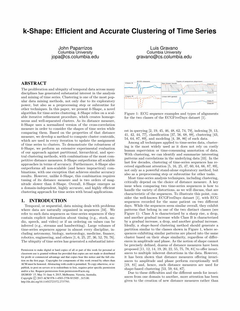
Figure 1: ECG sequence examples and types of alignmentsfor the two classes of the ECGFiveDays dataset [1].

est in querying [2, 19, 45, 46, 48, 62, 74, 79], indexing [9, 13,41, 42, 44, 77], classification [37, 56, 68, 88], clustering [43,54, 64, 87, 89], and modeling [4, 38, 86] of such data.Among all techniques applied to time-series data, cluster-

ing is the most widely used as it does not rely on costlyhuman supervision or time-consuming annotation of data.With clustering, we can identify and summarize interestingpatterns and correlations in the underlying data [33]. In thelast few decades, clustering of time-series sequences has re-ceived significant attention [5, 16, 25, 47, 60, 64, 66, 87, 89],not only as a powerful stand-alone exploratory method, butalso as a preprocessing step or subroutine for other tasks.Most time-series analysis techniques, including clustering,

critically depend on the choice of distance measure. A keyissue when comparing two time-series sequences is how tohandle the variety of distortions, as we will discuss, that arecharacteristic of the sequences. To illustrate this point, con-sider the well-known ECGFiveDays dataset [1], with ECGsequences recorded for the same patient on two differentdays. While the sequences seem similar overall, they exhibitpatterns that belong in one of the two distinct classes (seeFigure 1): Class A is characterized by a sharp rise, a drop,and another gradual increase while Class B is characterizedby a gradual increase, a drop, and another gradual increase.Ideally, a shape-based clustering method should generate apartition similar to the classes shown in Figure 1, where se-quences exhibiting similar patterns are placed into the samecluster based on their shape similarity, regardless of differ-ences in amplitude and phase. As the notion of shape cannotbe precisely defined, dozens of distance measures have beenproposed [11, 12, 14, 19, 20, 22, 55, 75, 78, 81] to offer invari-ances to multiple inherent distortions in the data. However,it has been shown that distance measures offering invari-ances to amplitude and phase perform exceptionally well[19, 81] and, hence, such distance measures are used forshape-based clustering [53, 59, 64, 87].Due to these difficulties and the different needs for invari-

ances from one domain to another, more attention has beengiven to the creation of new distance measures rather than

to the creation of new clustering algorithms. It is generallybelieved that the choice of distance measure is more im-portant than the clustering algorithm itself [7]. As a conse-quence, time-series clustering relies mostly on classic cluster-ing methods, either by replacing the default distance mea-sure with one that is more appropriate for time series, orby transforming time series into “flat” data so that existingclustering algorithms can be directly used [83]. However, thechoice of clustering method can affect: (i) accuracy, as ev-ery method expresses homogeneity and separation of clus-ters differently; and (ii) efficiency, as the computational costdiffers from one method to another. For example, spectralclustering [21] or certain variants of hierarchical clustering[40] are more appropriate to identify density-based clusters(i.e., areas of higher density than the remainder of the data)than partitional methods such as k-means [50] or k-medoids[40]. On the other hand, k-means is more efficient than hi-erarchical, spectral, or k-medoids methods.Unfortunately, state-of-the-art approaches for shape-based

clustering, which use partitional methods with distance mea-sures that are scale- and shift-invariant, suffer from twomain drawbacks: (i) these approaches cannot scale to large-volumes of data as they depend on computationally expen-sive methods or distance measures [53, 59, 64, 87]; (ii) theseapproaches have been developed for particular domains [87]or their effectiveness has only been shown for a limitednumber of datasets [53, 59]. Moreover, the most success-ful shape-based clustering methods handle phase invariancethrough a local, non-linear alignment of the sequence coor-dinates, even though a global alignment is often adequate.For example, for the ECG dataset in Figure 1, an efficientlinear drift can reveal the underlying differences in patternsof sequences of two classes, whereas an expensive non-linearalignment might match every corresponding increase or dropof each sequence, making it difficult to distinguish the twoclasses (see Figure 1). Importantly, to the best of our knowl-edge, these approaches have never been extensively evalu-ated against each other, against other partitional methods,or against different approaches such as hierarchical or spec-tral methods. We present such an experimental evaluationin this paper, as discussed below.In this paper, we propose k-Shape, a novel algorithm for

shape-based time-series clustering that is efficient and do-main independent. k-Shape is based on a scalable iterativerefinement procedure similar to the one used by the k-meansalgorithm, but with significant differences. Specifically, k-Shape uses both a different distance measure and a differentmethod for centroid computation from those of k-means. Asargued above, k-Shape attempts to preserve the shapes oftime-series sequences while comparing them. To do so, k-Shape requires a distance measure that is invariant to scal-ing and shifting. Unlike other clustering approaches [53, 64,87], for k-Shape we adapt the cross-correlation statisticalmeasure and we show: (i) how we can derive in a principledmanner a time-series distance measure that is scale- andshift-invariant; and (ii) how this distance measure can becomputed efficiently. Based on the properties of the normal-ized version of cross-correlation, we develop a novel methodto compute cluster centroids, which are used in every itera-tion to update the assignment of time series to clusters.To demonstrate the effectiveness of the distance measure

and k-Shape, we have conducted an extensive experimentalevaluation on 48 datasets and compared the state-of-the-artdistance measures and clustering approaches for time seriesusing rigorous statistical analysis. We took steps to ensurethe reproducibility of our results, including making available

our source code as well as using public datasets. Our resultsshow that our distance measure is competitive, outperform-ing Euclidean distance (ED) [20], and achieving similar re-sults as constrained Dynamic Time Warping (cDTW) [72],the best performing distance measure [19, 81], without re-quiring any tuning and performing one order of magnitudefaster. For example, for the ECG dataset in Figure 1, ourdistance measure achieves a one-nearest-neighbor classifica-tion accuracy of 98.9%, significantly higher than cDTW’saccuracy for the task, namely, 79.7%.For clustering, we show that the k-means algorithm with

ED, in contrast to what has been reported in the literature,is a robust approach and that inadequate modifications ofthe distance measure and the centroid computation can re-duce its performance. Moreover, simple partitional methodsoutperform hierarchical and spectral methods with the mostcompetitive distance measures, indicating that the choice ofalgorithm, which is sometimes believed to be less importantthan that of distance measure, is as critical as the choice ofdistance measure. Similarly, we show that k-Shape outper-forms all scalable and non-scalable partitional, hierarchical,and spectral methods in terms of accuracy, with the onlyexception of one existing approach that achieves similar re-sults, namely, k-medoids with cDTW. However, there areproblems with this approach that can be avoided with k-Shape: (i) the requirement of k-medoids to compute the dis-similarity matrix makes it unable to scale and particularlyslow, two orders of magnitude slower than k-Shape; (ii) itsdistance measure requires tuning, either through automatedmethods that rely on labeling of instances or through thehelp of a domain expert; this requirement is problematic forclustering, which is an unsupervised task. In contrast, k-Shape uses a simple, parameter-free distance measure. Over-all, k-Shape is a highly accurate and scalable choice for time-series clustering that performs exceptionally well across dif-ferent domains. k-Shape is particularly effective for applica-tions involving similar but out-of-phase sequences, such asthose of the ECG dataset in Figure 1, for which k-Shapereaches an 84% clustering accuracy, which is significantlyhigher than the 53% accuracy for k-medoids with cDTW.In this paper, we start with an in-depth review of the

state of the art for clustering time series, as well as with aprecise definition of our problem of focus (Section 2). Wethen present our novel approach as follows:• We show how a scale-, translate-, and shift-invariant dis-tance measure can be derived in a principled mannerfrom the cross-correlation measure and how this mea-sure can be efficiently computed (Section 3.1).• We present a novel method to compute a cluster centroidwhen that distance measure is used (Section 3.2).• We develop k-Shape, a centroid-based algorithm for time-series clustering (Section 3.3).• We evaluate our ideas by conducting an extensive exper-imental evaluation (Sections 4 and 5).

We conclude with a discussion of related work (Section 6)and the implications of our work (Section 7).

2. PRELIMINARIESIn this section, we review the relevant theoretical back-

ground (Section 2.1). We discuss distortions that are com-mon in time series (Section 2.2) and the most popular dis-tance measures for such data (Section 2.3). Then, we sum-marize existing approaches for clustering time-series data(Section 2.4) and for centroid computation (Section 2.5). Fi-nally, we formally present our problem of focus (Section 2.6).

2.1 Theoretical BackgroundHardness of clustering: Clustering is the general prob-

lem of partitioning n observations into k clusters, where acluster is characterized with the notions of homogeneity —the similarity of observations within a cluster — and sep-aration — the dissimilarity of observations from differentclusters. Even though many clustering criteria to capturehomogeneity and separation have been proposed [35], theminimum within-cluster sum of squared distances is mostcommonly used as it expresses both of them. Given a setof n observations X = {~x1, . . . ,~xn}, where ~xi ∈ Rm, and thenumber of clusters k < n, the objective is to partition X intok pairwise-disjoint clusters P = {p1, . . . ,pk}, such that thewithin-cluster sum of squared distances is minimized:

P ∗ = argminP

k∑j=1

∑~xi∈pj

dist(~xi,~cj)2 (1)

where ~cj is the centroid of partition pj ∈ P . In Euclideanspace this is an NP-hard optimization problem for k≥ 2 [3],even for number of dimensions m= 2 [51]. Because findinga global optimum is difficult, heuristics such as the k-meansmethod [50] are often used to find a local optimum. Specifi-cally, k-means randomly assigns the data points into k clus-ters and then uses an iterative procedure that performs twosteps in every iteration: (i) in the assignment step, everydata point is assigned to the cluster of its nearest centroid,which is determined with the use of a distance function; (ii)in the refinement step, the centroids of the clusters are up-dated to reflect the changes in cluster memberships. Thealgorithm converges either when there is no change in clus-ter memberships or when the maximum number of iterationsis reached.Steiner’s sequence: In the refinement step, k-means com-putes new centroids to serve as representatives of the clus-ters. The centroid is defined as the data point that mini-mizes the sum of squared distances to all other data pointsand, hence, it depends on the distance measure used. Find-ing such a centroid is known as the Steiner’s sequence prob-lem [63]: given a partition pj ∈ P , the corresponding cen-troid ~cj needs to fulfill:

~cj = argmin~w

∑~xi∈pj

dist(~w,~xi)2, ~w ∈ Rm (2)

When ED is used, the centroid can be computed with thearithmetic mean property [18]. In many cases where align-ment of observations is required, this problem is referred toas the multiple sequence alignment problem, which is knownto be NP-complete [80]. In the context of time series, Dy-namic Time Warping (DTW) (see Section 2.3) is the mostwidely used measure to compare time-series sequences withalignment, and many heuristics have been proposed to findthe average sequence under DTW (see Section 2.5).

2.2 Time-Series InvariancesBased on the domain, sequences are often distorted in

some way, and distance measures need to satisfy a numberof invariances in order to compare sequences meaningfully.In this section, we review common time-series distortionsand their invariances. For a more detailed review, see [7].Scaling and translation invariances: In many cases, itis useful to recognize the similarity of sequences despite dif-ferences in amplitude (scaling) and offset (translation). Inother words, transforming a sequence ~x as ~x′ = a~x+b, wherea and b are constants, should not change ~x’s similarity to

ED

DTW

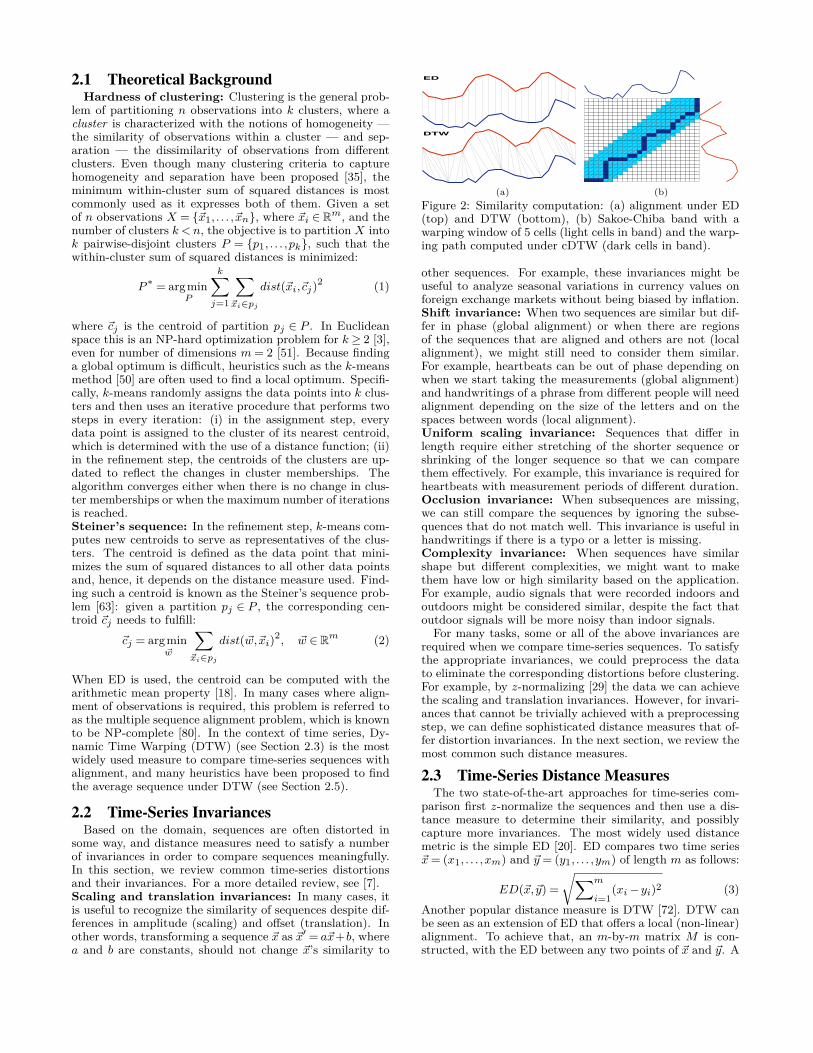
(a) (b)Figure 2: Similarity computation: (a) alignment under ED(top) and DTW (bottom), (b) Sakoe-Chiba band with awarping window of 5 cells (light cells in band) and the warp-ing path computed under cDTW (dark cells in band).

other sequences. For example, these invariances might beuseful to analyze seasonal variations in currency values onforeign exchange markets without being biased by inflation.Shift invariance: When two sequences are similar but dif-fer in phase (global alignment) or when there are regionsof the sequences that are aligned and others are not (localalignment), we might still need to consider them similar.For example, heartbeats can be out of phase depending onwhen we start taking the measurements (global alignment)and handwritings of a phrase from different people will needalignment depending on the size of the letters and on thespaces between words (local alignment).Uniform scaling invariance: Sequences that differ inlength require either stretching of the shorter sequence orshrinking of the longer sequence so that we can comparethem effectively. For example, this invariance is required forheartbeats with measurement periods of different duration.Occlusion invariance: When subsequences are missing,we can still compare the sequences by ignoring the subse-quences that do not match well. This invariance is useful inhandwritings if there is a typo or a letter is missing.Complexity invariance: When sequences have similarshape but different complexities, we might want to makethem have low or high similarity based on the application.For example, audio signals that were recorded indoors andoutdoors might be considered similar, despite the fact thatoutdoor signals will be more noisy than indoor signals.For many tasks, some or all of the above invariances are

required when we compare time-series sequences. To satisfythe appropriate invariances, we could preprocess the datato eliminate the corresponding distortions before clustering.For example, by z-normalizing [29] the data we can achievethe scaling and translation invariances. However, for invari-ances that cannot be trivially achieved with a preprocessingstep, we can define sophisticated distance measures that of-fer distortion invariances. In the next section, we review themost common such distance measures.

2.3 Time-Series Distance MeasuresThe two state-of-the-art approaches for time-series com-

parison first z-normalize the sequences and then use a dis-tance measure to determine their similarity, and possiblycapture more invariances. The most widely used distancemetric is the simple ED [20]. ED compares two time series~x= (x1, . . . ,xm) and ~y = (y1, . . . ,ym) of length m as follows:

ED(~x,~y) =√∑m

i=1(xi−yi)2 (3)

Another popular distance measure is DTW [72]. DTW canbe seen as an extension of ED that offers a local (non-linear)alignment. To achieve that, an m-by-m matrix M is con-structed, with the ED between any two points of ~x and ~y. A

warping pathW = {w1,w2, . . . ,wk}, with k≥m, is a contigu-ous set of matrix elements that defines a mapping between~x and ~y under several constraints [44]:

DTW (~x,~y) = min

√∑k

i=1wi (4)

This path can be computed on matrixM with dynamic pro-gramming for the evaluation of the following recurrence:γ(i, j) =ED(i, j)+min{γ(i−1, j−1),γ(i−1, j),γ(i, j−1)}.It is common practice to constrain the warping path tovisit only a subset of cells on matrix M . The shape of thesubset matrix is called band and the width of the band iscalled warping window. The most frequently used band forconstrained Dynamic Time Warping (cDTW) is the Sakoe-Chiba band [72]. Figure 2a shows the difference in align-ments of two sequences offered by ED and DTW distancemeasures, whereas Figure 2b presents the computation ofthe warping path (dark cells) for cDTW constrained by theSakoe-Chiba band with width 5 cells (light cells).Recently, Wang et al. [81] extensively evaluated 9 distance

measures and several variants thereof. They found that EDis the most efficient measure with a reasonably high accu-racy, and that DTW and cDTW perform exceptionally wellin comparison to other measures. cDTW is slightly betterthan DTW and significantly reduces the computation time.Several optimizations have been proposed to further speedup cDTW [65]. In the next section, we review clusteringalgorithms that can utilize these distance measures.

2.4 Time-Series Clustering AlgorithmsSeveral methods have been proposed to cluster time se-

ries. All approaches generally modify existing algorithms,either by replacing the default distance measures with aversion that is more suitable for comparing time series (raw-based methods), or by transforming the sequences into “flat”data so that they can be directly used in classic algorithms(feature- and model-based methods) [83]. Raw-based ap-proaches can easily leverage the vast literature on distancemeasures (see Section 2.3), which has shown that invari-ances offered by certain measures, such as DTW, are gen-eral and, hence, suitable for almost every domain [19]. Incontrast, feature- and model-based approaches are usuallydomain-dependent and applications on different domains re-quire that we modify the features or models. Because ofthese drawbacks of feature- and model-based methods, inthis paper we follow a raw-based approach.The three most popular raw-based methods are agglomer-

ative hierarchical, spectral, and partitional clustering [7]. Forhierarchical clustering, the most widely used “linkage” cri-teria are the single, average, and complete linkage vari-ants [40]. Spectral clustering [58] has recently started re-ceiving attention [7] due to its success over other types ofdata [21]. Among partitional methods, k-means [50] and k-medoids [40] are the most representative examples. Whenpartitional methods use distance measures that offer invari-ances to scaling, translation, and shifting, we consider themas shape-based approaches. From these methods, k-medoidsis usually preferred [83]: unlike k-means, k-medoids com-putes the dissimilarity matrix of all data sequences anduses actual sequences as cluster centroids; in contrast, k-means requires the computation of artificial sequences ascentroids, which hinders the easy adaptation of distancemeasures other than ED (see Section 2.1). However, fromall these methods, only the k-means class of algorithms canscale linearly with the size of the datasets. Recently, k-means was modified to work with: (i) the DTW distance

measure [64] and (ii) a distance measure that offers pair-wise scaling and shifting of time-series sequences [87]. Bothof these modifications rely on new approaches to computecluster centroids that we will review next.

2.5 Time-Series Averaging TechniquesThe computation of an average sequence or, in the context

of clustering, a centroid, is a difficult task and it criticallydepends on the distance measure used to compare time se-ries (see Section 2.1). We now review the state-of-the-artmethods for the computation of an average sequence.With Euclidean distance, the property of arithmetic mean

is used to compute an average sequence (e.g., as is the case inthe centroid computation of the k-means algorithm). How-ever, as DTW is more appropriate for many time-seriestasks [44, 65], several methods have been proposed to aver-age time-series sequences under DTW. Nonlinear alignmentand averaging filters (NLAAF) [32] uses a simple pairwisemethod where each coordinate of the average sequence is cal-culated as the center of the mapping produced by DTW. Thismethod is applied sequentially to pairs of sequences un-til only one pair is left. Prioritized shape averaging (PSA)[59] uses a hierarchical method to average sequences. Thecoordinates of an average sequence are computed as theweighted center of the coordinates of two time-series se-quences that were coupled by DTW. Initially, all sequenceshave weight one, and each average sequence produced in thenodes of the tree has a weight that corresponds to the num-ber of sequences it averages. To avoid the high computationcost of previous approaches, Ranking Shape-based TemplateMatching Framework (RSTMF) [53] approximates an order-ing of the time-series sequences by looking at the distancesof sequences to all other cluster centroids, instead of com-puting the distances of all pairs of sequences.Several drawbacks of these methods have led to the cre-

ation of a more robust technique called Dynamic TimeWarp-ing Barycenter Averaging (DBA) [64], which iteratively re-fines the coordinates of a sequence initially picked from thedata. Each coordinate of the average sequence is updatedwith the use of barycenter1 of one or more coordinates of theother sequences that were associated with the use of DTW.Among all these methods, DBA seems to be the most effi-cient and accurate averaging approach when DTW is used[64]. Another averaging technique that is based on matrixdecomposition was proposed as part of K-Spectral CentroidClustering (KSC) [87], to compute the centroid of a clusterwhen a distance measure for pairwise scaling and shifting isused. In our approach, which we will present in Section 3,we also rely on matrix decomposition to compute centroids.

2.6 Problem DefinitionWe address the problem of domain-independent, accurate,

and scalable clustering of time series into k clusters, for agiven value of the target number of clusters k.2 Even thoughdifferent domains might require different invariances to datadistortions (see Section 2.2), we focus on distance measuresthat offer invariances to scaling and shifting, which are gen-erally sufficient (see Section 2.3) [19]. Furthermore, to easilyadopt such distance measures, we focus our analysis on raw-based clustering approaches, as we argued in Section 2.4.Next, we introduce k-Shape, our novel clustering algorithm.1Barycenter is defined as b(X1, . . . ,Xa) = X1+...+Xa

a , where the sumsin the numerator are vector additions.2Although the exact estimation of k is difficult without a gold stan-dard, we can do so by varying k and evaluating clustering qualitywith criteria that capture information intrinsic to the data alone [40].

3. K-SHAPE CLUSTERING ALGORITHMOur objective is to develop a domain-independent, accu-

rate, and scalable algorithm for time-series clustering, witha distance measure that is invariant to scaling and shifting.We propose k-Shape, a novel centroid-based clustering algo-rithm that can preserve the shapes of time-series sequences.Specifically, we first discuss our distance measure, which isbased on the cross-correlation measure (Section 3.1). Basedon this distance measure, we propose a method to computecentroids of time-series clusters (Section 3.2). Finally, wedescribe our k-Shape clustering algorithm, which relies onan iterative refinement procedure that scales linearly in thenumber of sequences and generates homogeneous and well-separated clusters (Section 3.3).

3.1 Time-Series Shape SimilarityAs discussed earlier, capturing shape-based similarity re-

quires distance measures that can handle distortions in am-plitude and phase. Unfortunately, the best performing dis-tance measures offering invariances to these distortions, suchas DTW, are computationally expensive (see Section 2.3).To circumvent this efficiency limitation, we adopt a normal-ized version of the cross-correlation measure.Cross-correlation is a measure of similarity for time-lagged

signals that is widely used for signal and image process-ing. However, cross-correlation, a measure that comparesone-to-one points between signals, has largely been ignoredin experimental evaluations for the problem of time-seriescomparison. Instead, starting with the application of DTWdecades ago [8], research on that problem has focused onelastic distance measures that compare one-to-many or one-to-none points [11, 12, 44, 55, 78]. In particular, recentcomprehensive and independent experimental evaluations ofstate-of-the-art distance measures for time-series compar-ison — 9 measures and their variants in [19, 81] and 48measures in [26] — did not consider cross-correlation. Dif-ferent needs from one domain or application to another hin-der the process of finding appropriate normalizations for thedata and the cross-correlation measure. Moreover, ineffi-cient implementations of cross-correlation can make it ap-pear as slow as DTW. As a consequence of these drawbacks,cross-correlation has not been widely adopted as a time-series distance measure. In the rest of this section, we showhow to address these drawbacks. Specifically, we will showhow to choose normalizations that are domain-independentand efficient, and lead to a shape-based distance measurefor comparing time series efficiently and effectively.Cross-correlation measure: Cross-correlation is a statis-tical measure with which we can determine the similarity oftwo sequences ~x= (x1, . . . ,xm) and ~y = (y1, . . . ,ym), even ifthey are not properly aligned.3 To achieve shift-invariance,cross-correlation keeps ~y static and slides ~x over ~y to com-pute their inner product for each shift s of ~x. We denote ashift of a sequence as follows:

~x(s) =

(|s|︷ ︸︸ ︷

0, . . . ,0,x1,x2, . . . ,xm−s), s≥ 0(x1−s, . . . ,xm−1,xm,0, . . . ,0︸ ︷︷ ︸

|s|

), s < 0 (5)

When all possible shifts ~x(s) are considered, with s∈ [−m,m],we produce CCw(~x,~y) = (c1, . . . , cw), the cross-correlationsequence with length 2m−1, defined as follows:3For simplicity, we consider sequences of equal length even thoughcross-correlation can be computed on sequences of different length.

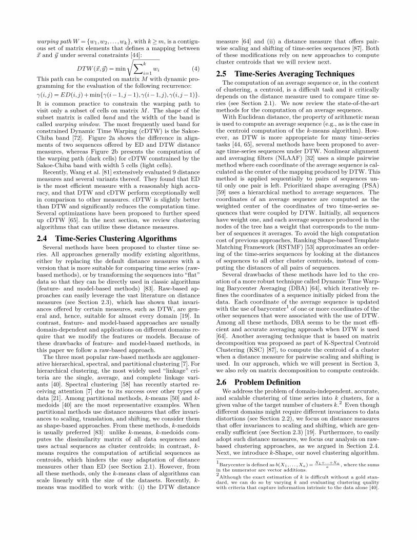
0 200 400 600 800 1,024−1.5

−1.0

−0.5

0

0.5

1.0

1.5

2.0

(a) z-normalized time series0 500 1,000 1,500 2,047

−30

−20

−10

0

10

20

30

X: 1797

Y: 27.3

(b) NCCb (no z-normalization)

0 500 1,000 1,500 2,047−1.5

−1.0

−0.5

0

0.5

1.0

1.5

X: 1694

Y: 1.08

(c) NCCu with z-normalization0 500 1,000 1,500 2,047

−0.4

−0.2

0

0.2

0.4

0.6

0.8

1.0

X: 1024

Y: 0.90

(d) NCCc with z-normalization

Figure 3: Time-series and cross-correlation normalizations.

CCw(~x,~y) =Rw−m(~x,~y), w ∈ {1,2, . . . ,2m−1} (6)where Rw−m(~x,~y) is computed, in turn, as:

Rk(~x,~y) =

m−k∑l=1

xl+k ·yl, k ≥ 0

R−k(~y,~x), k < 0(7)

Our goal is to compute the position w at which CCw(~x,~y)is maximized. Based on this value of w, the optimal shift of~x with respect to ~y is then ~x(s), where s= w−m.Depending on the domain or the application, different

normalizations for CCw(~x,~y) might be required. The mostcommon normalizations are the biased estimator, NCCb,the unbiased estimator, NCCu, and the coefficient normal-ization, NCCc, which are defined as follows:

NCCq(~x,~y) =

CCw(~x,~y)

m , q = “b” (NCCb)CCw(~x,~y)m−|w| , q = “u” (NCCu)CCw(~x,~y)√

R0(~x,~x)·R0(~y,~y), q = “c” (NCCc)

(8)

Beyond the cross-correlation normalizations, time seriesmight also require normalization to remove inherent distor-tions. Figure 3 illustrates how the cross-correlation normal-izations for two sequences ~x and ~y of length m = 1024 areaffected by time-series normalizations. (Appendix A alsoelaborates on the classification accuracy of cross-correlationvariants under other time-series normalizations.) Indepen-dently of the normalization applied to CCw(~x,~y), the pro-duced sequence will have length 2047. Initially, in Figure 3a,we remove differences in amplitude by z-normalizing ~x and ~yin order to show that they are aligned and, hence, no shiftingis required. If CCw(~x,~y) is maximized for w ∈ [1025,2047](or w ∈ [1,1023]), one of ~x or ~y should be shifted by i−1024to the right (or 1024− i to the left). Otherwise, if w = 1024,~x and ~y are properly aligned, which is what we expect in ourexample. Figure 3b shows that if we do not z-normalize ~xand ~y, and we use the biased estimator, then NCCb is max-imized at w = 1797, which indicates a shifting of a sequenceto the left 1797−1024 = 773 times. If we z-normalize ~x and~y, and use the unbiased estimator, then NCCu is maximizedat w = 1694, which indicates a shifting of a sequence to theright 1694− 1024 = 670 times (Figure 3c). Finally, if wez-normalize ~x and ~y, and use the coefficient normalization,then NCCc is maximized at w = 1024, which indicates thatno shifting is required (Figure 3d).As illustrated by the example above, normalizations of

the data and the cross-correlation measure can have a sig-

Algorithm 1: [dist,y′] = SBD(x,y)Input: Two z-normalized sequences x and yOutput: Dissimilarity dist of x and y

Aligned sequence y′ of y towards x1 length = 2nextpower2(2∗length(x)−1)

2 CC = IFFT{FFT(x, length)∗FFT(y, length)} // Equation 123 NCCc = CC

||x|| ||y|| // Equation 84 [value, index] = max(NCCc)5 dist = 1 −value // Equation 96 shift = index− length(x)7 if shift ≥ 0 then8 y′ = [zeros(1 ,shift),y(1 : end− shift)] // Equation 5

9 else10 y′ = [y(1 − shift : end),zeros(1 ,−shift)] // Equation 5

nificant impact on the cross-correlation sequence produced,which makes the creation of a distance measure a non-trivialtask. Furthermore, as we have seen in Figure 3, cross-correlation sequences produced by pairwise comparisons ofmultiple time series will differ in amplitude based on thenormalizations. Thus, a normalization that produces valueswithin a specified range should be used in order to mean-ingfully compare such sequences.Shape-based distance (SBD): To devise a shape-baseddistance measure, and based on the previous discussion, weuse the coefficient normalization that gives values between−1 and 1, regardless of the data normalization. Coeffi-cient normalization divides the cross-correlation sequence bythe geometric mean of autocorrelations of the individual se-quences. After normalization of the sequence, we detect theposition w where NCCc(~x,~y) is maximized and we derivethe following distance measure:

SBD(~x,~y) = 1−maxw

(CCw(~x,~y)√

R0(~x,~x) ·R0(~y,~y)

)(9)

which takes values between 0 to 2, with 0 indicating perfectsimilarity for time-series sequences.Up to now we have addressed shift invariance. For scaling

invariance, we transform each sequence ~x into ~x′ = ~x−µσ , so

that its mean µ is zero and its standard deviation σ is one.Efficient computation of SBD: From Equation 6, thecomputation of CCw(~x,~y) for all values of w requires O(m2)time, where m is the time-series length. The convolutiontheorem [39] states that the convolution of two time seriescan be computed as the Inverse Discrete Fourier Transform(IDFT) of the product of the individual Discrete FourierTransforms (DFT) of the time series, where DFT is:

F(xk) =|~x|−1∑r=0

xre−2jrkπ|~x| , k = 0, . . . , |~x|−1 (10)

and IDFT is:

F−1(xr) = 1|~x|

|~x|−1∑k=0

F(xk)e2jrkπ|~x| , r = 0, . . . , |~x|−1 (11)

where j =√−1. Cross-correlation is then computed as the

convolution of two time series if one sequence is first reversedin time, ~x(t) = ~x(−t) [39], which equals taking the complexconjugate (represented by ∗) in the frequency domain. Thus,Equation 6 can be computed for every m as:

CC(~x,~y) = F−1{F(~x)∗F(~y)} (12)However, DFT and IDFT still require O(m2) time. By usinga Fast Fourier Transform (FFT) algorithm [15], the time re-duces toO(m log(m)). Data and cross-correlation normaliza-tions can also be efficiently computed; thus the overall time

30 40 50 60 70 80 90 100

Arithmetic meanShape extraction

Class A

30 40 50 60 70 80 90 100

Class B

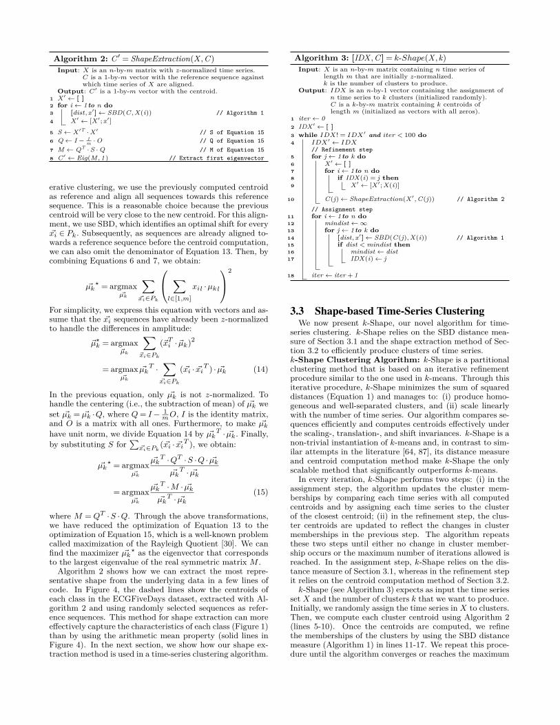
Figure 4: Examples of centroids for each class of the ECG-FiveDays dataset, based on the arithmetic mean property(solid lines) and our shape extraction method (dashed lines).

complexity of SBD remains O(m log(m)). Moreover, recur-sive algorithms compute an FFT by dividing it into piecesof power-of-two size [24]. Therefore, to further improve theperformance of the FFT computation, when CC(~x,~y) is notan exact power of two we pad ~x and ~y with zeros to reach thenext power-of-two length after 2m− 1. Algorithm 1 showshow this efficient and parameter-free measure is computedin a few lines of code using modern mathematical software.In this section, we showed effective cross-correlation and

data normalizations to derive a shape-based distance mea-sure. Importantly, we also discussed how the cross-correlationdistance measure can be efficiently computed. In our experi-mental evaluation (Sections 4 and 5), we will show that SBDis highly competitive, achieving similar results to cDTW andDTW while being orders of magnitude faster. We now turnto the critical problem of extracting a centroid for a cluster,to represent the cluster data consistently with the shape-based distance measure described above.

3.2 Time-Series Shape ExtractionMany tasks in time-series analysis rely on methods that ef-

fectively summarize a set of time series by only one sequence.This summary sequence is often referred to as an average se-quence or, in the context of clustering, as a centroid. Theextraction of meaningful centroids is a challenging task thatcritically depends on the choice of distance measure (seeSection 2.1). We now show how to determine such centroidsfor time-series clustering for the SBD distance measure, tocapture shared characteristics of the underlying data.The easiest way to extract an average sequence from a set

of sequences is to compute each coordinate of the averagesequence as the arithmetic mean of the corresponding coor-dinates of all sequences. This approach is used by k-means,the most popular clustering method. In Figure 4, the solidlines show such centroids for each class in the ECGFive-Days dataset of Figure 1: these centroids do not captureeffectively the class characteristics (see Figures 1 and 4).To avoid such problems, we cast the centroid computation

as an optimization problem where the objective is to find theminimizer of the sum of squared distances to all other timeseries sequences (Equation 2). However, as cross-correlationintuitively captures the similarity — rather than the dis-similarity — of time series, we can express the computedsequence as the maximizer µ?k of the squared similarities toall other time-series sequences. By rewriting Equation 2 asa maximization problem and from Equation 8, we obtain:

~µk? = argmax

~µk

∑~xi∈Pk

NCCc(~xi, ~µk)2

= argmax~µk

∑~xi∈Pk

(maxw CCw(~xi, ~µk)√R0(~xi, ~xi) ·R0( ~µk, ~µk)

)2

(13)

Equation 13 requires the computation of an optimal shift forevery ~xi ∈ Pk. As this approach is used in the context of it-

Algorithm 2: C ′ = ShapeExtraction(X ,C )Input: X is an n-by-m matrix with z-normalized time series.

C is a 1-by-m vector with the reference sequence againstwhich time series of X are aligned.

Output: C′ is a 1-by-m vector with the centroid.1 X′← [ ]2 for i← 1 to n do3 [dist,x′]← SBD(C ,X(i)) // Algorithm 14 X′← [X′;x′]

5 S← X′T ·X′ // S of Equation 156 Q← I − 1

m ·O // Q of Equation 157 M ←QT ·S ·Q // M of Equation 158 C ′← Eig(M,1) // Extract first eigenvector

erative clustering, we use the previously computed centroidas reference and align all sequences towards this referencesequence. This is a reasonable choice because the previouscentroid will be very close to the new centroid. For this align-ment, we use SBD, which identifies an optimal shift for every~xi ∈ Pk. Subsequently, as sequences are already aligned to-wards a reference sequence before the centroid computation,we can also omit the denominator of Equation 13. Then, bycombining Equations 6 and 7, we obtain:

~µk? = argmax

~µk

∑~xi∈Pk

∑l∈[1,m]

xil ·µkl

2

For simplicity, we express this equation with vectors and as-sume that the ~xi sequences have already been z-normalizedto handle the differences in amplitude:

~µ?k = argmax~µk

∑~xi∈Pk

(~xTi ·~µk)2

= argmax~µk

~µkT ·∑~xi∈Pk

(~xi · ~xiT ) · ~µk (14)

In the previous equation, only ~µk is not z-normalized. Tohandle the centering (i.e., the subtraction of mean) of ~µk weset ~µk = ~µk ·Q, where Q= I− 1

mO, I is the identity matrix,and O is a matrix with all ones. Furthermore, to make ~µkhave unit norm, we divide Equation 14 by ~µk

T · ~µk. Finally,by substituting S for

∑~xi∈Pk (~xi · ~xiT ), we obtain:

~µk? = argmax

~µk

~µkT ·QT ·S ·Q · ~µk

~µkT · ~µk

= argmax~µk

~µkT ·M · ~µk~µkT · ~µk

(15)

where M = QT ·S ·Q. Through the above transformations,we have reduced the optimization of Equation 13 to theoptimization of Equation 15, which is a well-known problemcalled maximization of the Rayleigh Quotient [30]. We canfind the maximizer ~µk

? as the eigenvector that correspondsto the largest eigenvalue of the real symmetric matrix M .Algorithm 2 shows how we can extract the most repre-

sentative shape from the underlying data in a few lines ofcode. In Figure 4, the dashed lines show the centroids ofeach class in the ECGFiveDays dataset, extracted with Al-gorithm 2 and using randomly selected sequences as refer-ence sequences. This method for shape extraction can moreeffectively capture the characteristics of each class (Figure 1)than by using the arithmetic mean property (solid lines inFigure 4). In the next section, we show how our shape ex-traction method is used in a time-series clustering algorithm.

Algorithm 3: [IDX ,C ] = k-Shape(X ,k)Input: X is an n-by-m matrix containing n time series of

length m that are initially z-normalized.k is the number of clusters to produce.

Output: IDX is an n-by-1 vector containing the assignment ofn time series to k clusters (initialized randomly).C is a k-by-m matrix containing k centroids oflength m (initialized as vectors with all zeros).

1 iter ← 02 IDX′← [ ]3 while IDX! = IDX′ and iter < 100 do4 IDX′← IDX

// Refinement step5 for j← 1 to k do6 X′← [ ]7 for i← 1 to n do8 if IDX(i) = j then9 X′← [X′;X(i)]

10 C(j)← ShapeExtraction(X′,C(j)) // Algorithm 2

// Assignment step11 for i← 1 to n do12 mindist←∞13 for j← 1 to k do14 [dist,x′]← SBD(C(j),X(i)) // Algorithm 115 if dist < mindist then16 mindist← dist17 IDX(i)← j

18 iter ← iter + 1

3.3 Shape-based Time-Series ClusteringWe now present k-Shape, our novel algorithm for time-

series clustering. k-Shape relies on the SBD distance mea-sure of Section 3.1 and the shape extraction method of Sec-tion 3.2 to efficiently produce clusters of time series.k-Shape Clustering Algorithm: k-Shape is a partitionalclustering method that is based on an iterative refinementprocedure similar to the one used in k-means. Through thisiterative procedure, k-Shape minimizes the sum of squareddistances (Equation 1) and manages to: (i) produce homo-geneous and well-separated clusters, and (ii) scale linearlywith the number of time series. Our algorithm compares se-quences efficiently and computes centroids effectively underthe scaling-, translation-, and shift invariances. k-Shape is anon-trivial instantiation of k-means and, in contrast to sim-ilar attempts in the literature [64, 87], its distance measureand centroid computation method make k-Shape the onlyscalable method that significantly outperforms k-means.In every iteration, k-Shape performs two steps: (i) in the

assignment step, the algorithm updates the cluster mem-berships by comparing each time series with all computedcentroids and by assigning each time series to the clusterof the closest centroid; (ii) in the refinement step, the clus-ter centroids are updated to reflect the changes in clustermemberships in the previous step. The algorithm repeatsthese two steps until either no change in cluster member-ship occurs or the maximum number of iterations allowed isreached. In the assignment step, k-Shape relies on the dis-tance measure of Section 3.1, whereas in the refinement stepit relies on the centroid computation method of Section 3.2.k-Shape (see Algorithm 3) expects as input the time series

set X and the number of clusters k that we want to produce.Initially, we randomly assign the time series in X to clusters.Then, we compute each cluster centroid using Algorithm 2(lines 5-10). Once the centroids are computed, we refinethe memberships of the clusters by using the SBD distancemeasure (Algorithm 1) in lines 11-17. We repeat this proce-dure until the algorithm converges or reaches the maximum

number of iterations (usually a small number, such as 100).The output of the algorithm is the assignment of sequencesto clusters and the centroids for each cluster.Complexity of k-Shape: As we claimed earlier, k-Shapescales linearly with the number of time series. To see why, wewill analyze the computational complexity of Algorithm 3,where n is the number of time series, k is the number ofclusters, and m is the length of the time series. In theassignment step, k-Shape computes the dissimilarity of ntime series to k centroids by using SBD, which requiresO(m · log(m)) time. Thus, the time complexity of this step isO(n ·k ·m · log(m)). In the refinement step, for every cluster,k-Shape computes matrix M , which requires O(m2) time,and performs an eigenvalue decomposition on M , which re-quires O(m3) time. Thus, the complexity of this step isO(max{n ·m2, k ·m3}). Overall, k-Shape requiresO(max{n ·k ·m · log(m), n ·m2, k ·m3}) time per iteration. We see thatthis algorithm has a linear dependence in the number of timeseries, and the majority of the computation cost depends onthe length of the time series. However, this length is usuallymuch smaller than the number of time series (i.e., m� n)and, hence, the dependence on m is not a bottleneck. (Ap-pendix B further examines the scalability of k-Shape.) Inrare cases where m is very large (i.e., m� n), segmenta-tion or dimensionality reduction approaches can be used tosufficiently reduce the length of the sequences [10, 49].We now turn to the experimental evaluation of k-Shape

against the state-of-the-art time-series clustering approaches.

4. EXPERIMENTAL SETTINGSIn this section, we describe the experimental settings for

the evaluation of both SBD and our k-Shape algorithm.Datasets: We use the largest public collection of class-labeled time-series datasets, namely, the UCR time-seriescollection [1]. It consists of 48 datasets,4 both synthetic andreal, which span several different domains. Each datasetcontains from 56 to 9236 sequences. The sequences in eachdataset have equal length, but from one dataset to anotherthe sequence length varies from 24 to 1882. These datasetsare annotated and every sequence can belong to only oneclass, which, in the context of clustering, should be inter-preted as the cluster where the sequence belongs. Further-more, the datasets are already z-normalized5 and split intotraining and test sets. As we will see, we use this split ofthe datasets for the distance measure evaluation; we also usethe training sets for tuning some of the baselines.Platform: We ran our experiments on a cluster of 10 serverswith identical configuration: Dual Intel Xeon X5550 (4-corewith 2-way SMT) processor with clock speed at 2.67 GHzand 24 GB RAM. We utilized up to 16 processes continu-ously for a period of two months in order to perform all ex-periments included in this paper. Each server runs Ubuntu12.04 (64-bit) and Matlab R2012b (64-bit).Implementation: We implemented our approach and allstate-of-the-art approaches that we compare against underthe same framework, in Matlab, for a consistent evaluationin terms of both accuracy and efficiency. For repeatabilitypurposes, we make all datasets and source code available.6

4Currently, 47 out of 48 datasets are listed in [1]. One dataset,namely, Insect, will become publicly available in the next release,according to the owners of the UCR repository [1].5Several datasets as available in [1] are not z-normalized. (We havecommunicated about this issue with the site owners.) Therefore, ourexperiments start with a z-normalization step for all datasets.6http://www.cs.columbia.edu/~jopa/kshape.html

Baselines: We evaluate both our distance measure, SBD,and our clustering approach, k-Shape. We compare SBDagainst the strongest state-of-the-art distance measures fortime series (see Section 2.3 for a detailed discussion):• ED: a simple, efficient — yet accurate — distance mea-sure for time series [20]• DTW: the best performing — but expensive — distancemeasure for time series [72]• cDTW: the constrained version of DTW, with improvedaccuracy and efficiency [72]

We compare k-Shape against the three strongest types ofscalable and non-scalable clustering methods, namely, par-titional, hierarchical, and spectral methods (see Section 2.4for a detailed discussion), combined with the most compet-itive distance measures. As scalable methods, we considerthe classic k-means algorithm with ED (k-AVG+ED) [50]and the following variants of k-means:• k-AVG+Dist: k-means with DTW and SBD as dis-tance measures and the arithmetic mean of time seriescoordinates for centroid computation• k-DBA: k-means with DTW as distance measure andthe DBA method for centroid computation [64]• KSC: k-means with a distance measure offering pairwisescaling and shifting of time series and computation of thespectral norm of a matrix (i.e., matrix decomposition)for centroid computation [87]

As non-scalable methods, among partitional methods weconsider the Partitioning Around Medoids (PAM) imple-mentation of the k-medoids algorithm [40]. Among hierar-chical methods, we use agglomerative hierarchical clusteringwith single, average, and complete linkage criteria [40]. Fi-nally, among spectral methods, we consider the popular nor-malized spectral clustering method [58]. These non-scalableapproaches require a large number of distance calculationsto compute the full dissimilarity matrix and, hence, they be-come unacceptably inefficient with high-cost distance mea-sures. For this reason, we ignore DTW and focus instead onED, cDTW, and SBD as distance measures. In Table 1 wesummarize the combinations used in our evaluation. Over-all, we compared k-Shape against 20 clustering approaches.Parameter settings: Among the distance measures dis-cussed above, only cDTW requires setting a parameter, toconstrain its warping window. We consider two cases fromthe literature: (i) cDTWopt: we compute the optimal win-dow by performing a leave-one-out classification step overthe training set of each dataset; (ii) cDTWw: we use aswindow 5%, for cDTW5, and 10%, for cDTW10, of thelength of the time series of each dataset; this second caseis more realistic for an unsupervised setting such as cluster-ing.7 For the 1-NN classification computation, we also con-sider the state-of-the-art lower bounding approach LBKeogh[44], which prunes time series unlikely for a match whenDTW and cDTW are used. We denote lower bounding withthe LB subscript (e.g., cDTW10

LB). For clustering, all thealgorithms that we compare, except for hierarchical cluster-ing, receive the target number of clusters k as input, whichis equal to the number of classes for each dataset. For hi-erarchical clustering, we compute a threshold that cuts theproduced dendrogram at the minimum height such that kclusters are formed. We set the maximum number of itera-tions for k-Shape, all variants of k-means, PAM, and spec-tral methods to 100. Finally, in every iteration of k-Shape,k-DBA, and KSC, we use the centroids of the previous run

7For non-scalable methods, we use cDTW5 for its efficiency, as notedin Table 1, even though cDTW10 and cDTWopt perform similarly.

Name Clustering Algorithm DistanceMeasure

PAM+ED Partitioning Around Medoids EDPAM+cDTW Partitioning Around Medoids cDTW5

PAM+SBD Partitioning Around Medoids SBDH-S+ED Hierarchical with single linkage EDH-A+ED Hierarchical with average linkage EDH-C+ED Hierarchical with complete linkage ED

H-S+cDTW Hierarchical with single linkage cDTW5

H-A+cDTW Hierarchical with average linkage cDTW5

H-C+cDTW Hierarchical with complete linkage cDTW5

H-S+SBD Hierarchical with single linkage SBDH-A+SBD Hierarchical with average linkage SBDH-C+SBD Hierarchical with complete linkage SBD

S+ED Normalized Spectral Clustering EDS+cDTW Normalized Spectral Clustering cDTW5

S+SBD Normalized Spectral Clustering SBD

Table 1: Combinations of PAM, hierarchical, and spectralmethods with ED, cDTW, and SBD for our evaluation.

as reference sequences to refine the centroids of the currentrun once.Metrics: We compare all approaches on both runtime andaccuracy. For runtime, we compute CPU time utilizationand report time ratios for our comparisons. Following [19],we use the 1-NN classifier, which is a simple and parameter-free classifier, to evaluate distance measures. We report theclassification accuracy (i.e., number of correctly classified in-stances over all instances) by performing 1-NN classificationover the training and test sets of each dataset. Because the1-NN classifier is deterministic, we make this computationonce. Following [7], we use the Rand Index [67] to evaluateclustering accuracy over the fused training and test sets ofeach dataset. This metric is related to the classification ac-curacy and is defined as R = TP+TN

TP+TN+FP+FN , where TPis the number of time series pairs that belong to the sameclass and are assigned to the same cluster, TN is the numberof time series pairs that belong to different classes and areassigned to different clusters, FP is the number of time se-ries pairs that belong to different classes but are assigned tothe same cluster, and FN is the number of time series pairsthat belong to the same class but are assigned to differentclusters. As hierarchical algorithms are deterministic, we re-port the Rand Index over one run. However, for partitionalmethods, we report the average Rand Index over 10 runsand for spectral methods the average Rand Index over 100runs; in every run we use a different random initialization.Statistical analysis: Following [7, 26], we analyze the re-sults of every pairwise comparison of algorithms over multi-ple datasets using the Wilcoxon test [84] with a 99% confi-dence level. According to [17], the Wilcoxon test is less af-fected by outliers than is the t-test [69], as Wilcoxon does notconsider absolute commensurability of differences. More-over, using pairwise tests to reason about multiple algo-rithms is not fully satisfactory because sometimes the nullhypotheses are rejected due to random chance. Therefore,we also use the Friedman test [23] followed by the post-hocNemenyi test [57] for comparison of multiple algorithms overmultiple datasets, as suggested in [17]. The Friedman andNemenyi tests require more evidence to detect statisticalsignificance than the Wilcoxon test [26] (i.e., the larger thenumber of methods, the larger the number of datasets re-quired) and, hence, as we already use all 48 datasets for theWilcoxon test, we report statistical significant results witha 95% confidence level.

5. EXPERIMENTAL RESULTSIn this section, we discuss our experiments. First, we

evaluate SBD against the state-of-the-art distance measures(Section 5.1). Then, we compare k-Shape against scalable(Section 5.2) and non-scalable (Section 5.3) clustering ap-proaches. Finally, we highlight our findings (Section 5.4).

5.1 Evaluation of SBDComparison against ED: To understand if SBD (Sec-

tion 3.1) is an effective measure for time-series comparison,we evaluate it against the state-of-the-art distance measures,using their 1-NN classification accuracies across 48 datasets(Section 4). Table 2 reports the performance of the state-of-the-art measures against the baseline ED. All distance mea-sures, including SBD, outperform ED with statistical signif-icance. For DTW, constraining its warping window signifi-cantly improves performance. In particular, cDTWopt per-forms at least as well as DTW in 36 datasets, cDTW5 per-forms at least as well as DTW in 34 datasets, and cDTW10

performs at least as well as DTW in 41 datasets. However,the statistical test suggests that there is no significant differ-ence between cDTWopt, cDTW5, and cDTW10. Figure 5afurther illustrates the superiority of SBD over ED.Comparison against DTW and cDTW: Figure 5b showsthat the difference in accuracy between SBD and DTW is inmost cases negligible: SBD performs at least as well as DTWin 30 datasets, but the statistical test reveals no evidencethat either measure is better than the other. Consideringthe constrained versions of DTW, we observe that SBD per-forms similarly to or better than cDTWopt, cDTW5, andcDTW10 in 22, 18, and 19 datasets, respectively. Inter-estingly, there is no significant difference between SBD andcDTW10, but cDTWopt and cDTW5 are significantly betterthan SBD. cDTWopt, with its optimal tuning, identifies thatacross the 48 datasets the average warping window is 4.5%.This explains why cDTW5 behaves similarly to cDTWopt

and outperforms SBD, whereas the large majority of con-strained cDTWw variants, including cDTW10, do not out-perform SBD. Importantly, the p-values for the Wilcoxontest between cDTWopt and SBD, and between cDTW5 andSBD, are close to the confidence level, which indicates thatdeeper statistical analysis is required, as we discuss next.Statistical analysis: To better understand the performanceof SBD in comparison with cDTWopt and cDTW5, we eval-uate the significance of their differences in accuracy whenconsidered all together. Figure 6 shows the average rankacross datasets of each distance measure. cDTWopt is thetop measure, with an average rank of 1.96, meaning thatcDTWopt performed best in the majority of the datasets.The Friedman test rejects the null hypothesis that all mea-sures behave similarly, and, hence, we proceed with a post-hoc Nemenyi test, to evaluate the significance of the differ-ences in the ranks. The wiggly line in the figure connectsall measures that do not perform statistically differently ac-cording to the Nemenyi test. We observe that the ranksof cDTWopt, cDTW5, and SBD do not present a signifi-cant difference, and ED, which is ranked last, is significantlyworse than the others. In conclusion, SBD is a very com-petitive distance measure that significantly outperforms EDand achieves similar results to both constraint and uncon-straint versions of DTW. Moreover, SBD is the most robustvariant of the cross-correlation measure (see Appendix A).Efficiency: We now show that SBD is not only competi-tive in terms of accuracy, but also highly efficient. We also

DistanceMeasure > = < Better Average

Accuracy Runtime

DTW 29 2 17 3 0.788 15573xDTWLB 6040xcDTWopt

31 15 2 3 0.814 2873xcDTWopt

LB322x

cDTW534 3 11 3 0.809 1558x

cDTW5LB

122xcDTW10

33 1 14 3 0.804 2940xcDTW10

LB364x

SBDNoFFT

30 12 6 3 0.795224x

SBDNoPow2 8.7xSBD 4.4x

Table 2: Comparison of distance measures. Columns “>”,“=”, and “<” denote the number of datasets over which adistance measure is better, equal, or worse, respectively, incomparison to ED. “Better” indicates that a distance mea-sure outperforms ED with statistical significance. “Averageaccuracy” denotes the accuracy achieved in the 48 datasetswhereas “Runtime” indicates the factor by which a distancemeasure is slower than ED.

demonstrate that implementation choices for SBD can sig-nificantly impact its speed. The last row of Table 2 showsthe factors by which each SBD variation is slower than ED.The optimized version of SBD, denoted simply as SBD, isthe fastest version, performing only 4.4x slower than ED.When we use SBD still with FFT but without the power-of-two-length optimization discussed in Section 3.1, the re-sulting measure, SBDNoPow2, is 8.7x slower than ED. Fur-thermore, SBDNoFFT , the version of SBD without FFT,is two orders of magnitude slower (224x) than ED and oneorder slower (51x) than SBD. Table 2 also shows that SBDis substantially faster than the DTW and cDTW variants.Specifically, SBD is three orders of magnitude (3533x) fasterthan DTW, two orders (652x) faster than cDTWopt, twoorders (353x) faster than cDTW5, and two orders (667x)faster than cDTW10. Even when we speed up the search of1-NN classification computation, by pruning time series un-likely for a match using LBKeogh, SBD is still significantlyfaster. In particular, SBD now becomes one order of mag-nitude faster (73x) than cDTWopt

LB , one order faster (28x)than cDTW5

LB , and one order faster (82.5x) than cDTW10LB ,

while remaining three orders faster (1370x) than DTWLB .

5.2 k-Shape Against Other Scalable MethodsComparison against k-AVG+ED: Having shown the

robustness of SBD, we now compare our algorithm, k-Shape,against scalable state-of-the-art time-series clustering algo-rithms. Table 3 reports the performance of variants of k-means against k-AVG+ED, using their Rand Index on the48 datasets (see Section 4). From all these variants of k-means, only k-Shape outperforms k-AVG+ED with statis-tical significance, and, in particular, k-Shape significantlyoutperforms every other method. In most cases, replacingED in k-means with other distance measures not only doesnot improve accuracy significantly, but in certain cases re-sults in substantially lower performance. For example, k-AVG+SBD achieves higher accuracy than k-AVG+ED in67% of the datasets, but the differences in accuracy are notstatistically significant. Interestingly, when DTW is com-bined with k-means, in k-AVG+DTW, the performance issignificantly worse than with k-AVG+ED. Even in caseswhere both the distance measure and the centroid computa-tion method of k-means are modified, the performance does

0.3 0.4 0.5 0.6 0.7 0.8 0.9 1.00.3

0.4

0.5

0.6

0.7

0.8

0.9

1.0

ED

SB

D

(a) SBD vs. ED

0.3 0.4 0.5 0.6 0.7 0.8 0.9 1.00.3

0.4

0.5

0.6

0.7

0.8

0.9

1.0

DTW

SB

D

(b) SBD vs. DTW

Figure 5: Comparison of SBD, ED, and DTW over 48datasets. Circles above the diagonal indicate datasets overwhich SBD has better accuracy than the compared method.

1 2 3 4

cDTWopt

cDTW5EDSBD

Figure 6: Ranking of distance measures based on the aver-age of their ranks across datasets. The wiggly line connectsall measures that do not perform statistically differently ac-cording to the Nemenyi test.

not improve significantly in comparison to k-AVG+ED. k-DBA outperforms k-AVG+DTWwith statistical significancein 39 out of 48 datasets. Both of these approaches use DTWas distance measure, but k-DBA also modifies its centroidcomputation method. This modification significantly im-proves the performance of k-DBA over that of k-AVG+DTW,with an average improvement in Rand Index of 25.6%. De-spite this improvement, k-DBA still does not perform betterthan k-AVG+ED in a statistical significant manner.8 An-other algorithm that modifies both the distance measure andthe centroid computation method of k-means is KSC. Simi-larly to k-DBA, KSC does not outperform k-AVG+ED.Comparison against k-DBA and KSC: Both k-DBAand KSC are similar to k-Shape in that they all modify boththe centroid computation method and the distance measureof k-means. Therefore, to understand the impact of thesemodifications, we compare them against our k-Shape algo-rithm (see Figure 7). k-Shape is better in 30 datasets andworse in 18 datasets in comparison to KSC (Figure 7a), andis better in 35 datasets and worse in 13 datasets in compar-ison to k-DBA (Figure 7b). In both of these comparisons,the statistical test indicates the superiority of k-Shape.Statistical analysis: In addition to the pairwise compar-isons performed with the Wilcoxon test, we further evaluatethe significance of the differences in algorithm performancewhen considered all together. Figure 8 shows the averagerank across datasets of each k-means variant. k-Shape isthe top technique, with an average rank of 1.89, meaningthat k-Shape achieved better rank in the majority of thedatasets. The Friedman test rejects the null hypothesis thatall algorithms behave similarly, and, hence, we proceed witha post-hoc Nemenyi test, to evaluate the significance of thedifferences in the ranks. We observe that the ranks of KSC,k-DBA, and k-AVG+ED do not present a statistically sig-nificant difference, whereas k-Shape, which is ranked first,is significantly better than the others. To conclude, modi-

8Even when multiple refinements of k-DBA’s centroids are performedper iteration, k-DBA still does not outperform k-AVG+ED. In par-ticular, performing five refinements per iteration improves the RandIndex by 4% but runtime increases by 30%.

Algorithm > = < Better Worse RandIndex Runtime

k-AVG+SBD 32 1 15 7 7 0.745 3.6xk-AVG+DTW 10 0 38 7 3 0.584 3444x

KSC 22 0 26 7 7 0.636 448xk-DBA 18 0 30 7 7 0.733 3892x

k-Shape+DTW 19 1 28 7 7 0.698 4175xk-Shape 36 1 11 3 7 0.772 12.4x

Table 3: Comparison of k-means variants against k-AVG+ED. Columns “>”, “=”, and “<” denote the num-ber of datasets over which an algorithm is better, equal,or worse, respectively, in comparison to k-AVG+ED. “Bet-ter” indicates that an algorithm outperforms k-AVG+EDwith statistical significance whereas “Worse” indicates thatk-AVG+ED outperforms an algorithm with statistical sig-nificance. “Rand Index” denotes the accuracy achieved inthe 48 datasets whereas “Runtime” indicates the factor bywhich an algorithm is slower than k-AVG+ED.

fying k-means with inappropriate distance measures or cen-troid computation methods might lead to unexpected re-sults. The same holds for k-Shape, where the use of DTW asits distance measure, in k-Shape+DTW, significantly dropsits performance (i.e., k-Shape outperforms k-Shape+DTWwith statistical significance in 36 out of 48 datasets).Efficiency: k-Shape is the only algorithm that outperformsall k-means variants, including the simple, yet robust, k-AVG+ED. We now investigate whether k-Shape’s superior-ity in terms of accuracy has an associated penalty in effi-ciency. Table 3 shows the factors by which each algorithmis slower than k-AVG+ED. Our approach, k-Shape, is oneorder of magnitude faster (36x) than KSC, two orders ofmagnitude faster (313x) than k-DBA, and 12.4x slower thank-AVG+ED.

5.3 k-Shape Against Non-Scalable MethodsComparison against k-AVG+ED: Up to now, we have

focused our evaluation on scalable clustering algorithms. Inorder to show the robustness of k-Shape in terms of accu-racy beyond scalable approaches, we now ignore scalabilityand compare k-Shape against clustering methods that scalequadratically with the number of time series, namely, hierar-chical, spectral, and k-medoids methods. Table 4 reports theperformance of non-scalable methods against k-AVG+ED.Among all existing state-of-the-art methods that use EDor cDTW as distance measures, only partitional methodsperform similarly to or better than k-AVG+ED. In partic-ular, PAM+cDTW is the only method that outperforms k-AVG+ED with statistical significance. PAM+ED achievesbetter performance in 63% of the datasets in comparisonto k-AVG+ED; however, this difference is not statisticallysignificant. Moreover, PAM+cDTW performs better in 33datasets, equal in 1 dataset, and worse in 14 datasets rela-tive to PAM+ED. For this comparison, the statistical sig-nificance test indicates the superiority of PAM+cDTW.All combinations of hierarchical clustering, with all dif-

ferent linkage criteria, perform poorly in comparison to k-AVG+ED. Interestingly, k-AVG+EDoutperformsall of themwith statistical significance. We observe that the major dif-ference in performance among hierarchical methods is thelinkage criterion and not the distance measure. This high-lights the importance of the clustering method and not onlyof the distance measure for time-series clustering. Simi-larly to hierarchical methods, spectral methods also per-form poorly against k-AVG+ED. S+cDTW performs betterin more datasets than S+ED in comparison to k-AVG+ED:

0.3 0.4 0.5 0.6 0.7 0.8 0.9 1.00.3

0.4

0.5

0.6

0.7

0.8

0.9

1.0

KSC

k−

Sh

ap

e

(a) k-Shape vs. KSC

0.3 0.4 0.5 0.6 0.7 0.8 0.9 1.00.3

0.4

0.5

0.6

0.7

0.8

0.9

1.0

k−DBA

k−

Shape

(b) k-Shape vs. k-DBA

Figure 7: Comparison of k-Shape, KSC, and k-DBA over 48datasets. Circles above the diagonal indicate datasets overwhich k-Shape has better Rand Index.

1 2 3 4

k-Shapek-AVG+ED

KSCk-DBA

Figure 8: Ranking of k-means variants based on the averageof their ranks across datasets. The wiggly line connectsall techniques that do not perform statistically differentlyaccording to the Nemenyi test.

comparing S+cDTW with S+ED, S+cDTW achieves sim-ilar or better accuracy in 27 datasets, but this differenceis not significant. Importantly, k-AVG+ED is significantlybetter than both S+ED and S+cDTW. Therefore, for hier-archical and spectral methods, these distance measures havea small impact on their performance.k-Shape against PAM+cDTW: Among all methods thatwe evaluated, only PAM+cDTW outperforms k-AVG+EDwith statistical significance. Therefore, we compare this ap-proach with k-Shape. PAM+cDTW is better in 31, equalin 1, and worse in 16 datasets in comparison to k-Shape,but this difference is not significant. For completeness, wealso evaluate SBD with hierarchical, spectral, and k-medoidsmethods. For hierarchical methods, H-C+SBD is betterthan H-A+SBD, and, in turn, H-A+SBD is better thanH-S+SBD, all with statistical significance. For each link-age option, there is no significance in the accuracy betweenED, SBD, and cDTW. S+SBD, in contrast to S+ED andS+cDTW, outperforms k-AVG+ED in 38 out of 48 datasets,with statistical significance. S+SBD is also significantly bet-ter than S+ED and S+cDTW, but S+SBD does not outper-form k-Shape. Similarly, PAM+SBD performs equally to orbetter than k-AVG+ED in 36 out of 48 datasets. The sta-tistical test suggests that PAM+SBD is significantly betterthan k-AVG+ED but not better than k-Shape.Statistical analysis: We evaluate the significance of thedifferences in algorithm performance for all algorithms thatsignificantly outperform k-AVG+ED. The Friedman test re-jects the null hypothesis that all algorithms behave simi-larly, and, hence, as before, we proceed with a post-hocNemenyi test. Figure 9 shows that k-Shape, PAM+SBD,PAM+cDTW, and S+SBD do not present a significant dif-ference in accuracy, whereas k-AVG+ED, which is rankedlast, is significantly worse than the others.From our extensive evaluation of existing scalable and

non-scalable clustering approaches for time series that useED, cDTW, or DTW as distance measures, PAM+cDTW isthe only approach that achieves similar — but not better —results to k-Shape. In contrast to k-Shape, PAM+cDTWhas two drawbacks that make it an unrealistic choice fortime-series clustering: (i) its distance measure, cDTW, re-

Algorithm > = < Better Worse RandIndex

H-S+ED 3 1 44 7 3 0.328H-S+cDTW 7 0 41 7 3 0.371

H-S+SBD 6 1 41 7 3 0.349H-A+ED 3 1 44 7 3 0.599

H-A+cDTW 9 0 39 7 3 0.617H-A+SBD 8 0 40 7 3 0.541H-C+ED 8 0 40 7 3 0.690

H-C+cDTW 15 0 33 7 3 0.699H-C+SBD 17 0 31 7 3 0.697

S+ED 7 1 40 7 3 0.602S+cDTW 18 1 29 7 3 0.563

S+SBD 38 0 10 3 7 0.769PAM+ED 30 1 17 7 7 0.762

PAM+cDTW 38 1 9 3 7 0.772PAM+SBD 35 1 12 3 7 0.780

Table 4: Comparison of hierarchical, spectral, and k-medoids variants against k-AVG+ED. Columns “>”, “=”,and “<” denote the number of datasets over which an algo-rithm is better, equal, or worse, respectively, in comparisonto k-AVG+ED. “Better” indicates that an algorithm out-performs k-AVG+ED with statistical significance whereas“Worse” indicates that k-AVG+ED outperforms an algo-rithm with statistical significance. “Rand Index” denotesthe accuracy achieved in the 48 datasets.

quires tuning to improve its performance and reduce thecomputation cost; and (ii) the computation of the dissimi-larity matrix that PAM+cDTW requires as input makes itunable to scale in both time and space. For example, the ma-trix computation alone is already two orders of magnitudeslower than the computation required by k-Shape. Thus,k-Shape emerges as a domain-independent, highly accurate,and scalable approach for time-series clustering.

5.4 Summary of ResultsIn short, our experimental evaluation suggests that: (1)

cross-correlation measures (e.g., SBD), which are not widelyadopted as time-series distance measures, are as competitiveas state-of-the-art measures, such as cDTW and DTW, butsignificantly faster; (2) the k-means algorithm with ED, incontrast to what has been reported in the literature, is arobust approach for time-series clustering, but inadequatemodifications of its distance measure and centroid computa-tion can reduce its performance; (3) the choice of clusteringmethod, which was believed to be less important than thatof distance measure, is as important as the choice of distancemeasure; and overall (4) k-Shape is a highly accurate andefficient method for time-series clustering.

6. RELATED WORKThis paper focused on efficient and domain-independent

time-series clustering. Section 2 provided an in-depth dis-cussion of the state of the art for time-series clustering,which we will not repeat for brevity. Specifically, Section 2.1summarized the relevant theoretical background, Section 2.2reviewed common distortions in time series, and Section 2.3discussed the most popular state-of-the-art distance mea-sures for time series. (We refer the reader to [19, 81] fora thorough review and evaluation of the alternative time-series distance measures.) Section 2.4 highlighted existingapproaches for clustering time series. (We refer the reader to[83] for a more detailed view of these approaches.) Finally,Section 2.5 discussed the methods for centroid computationthat are part of many time-series clustering algorithms.As argued throughout the paper, we focus on shape-based

clustering of time series. Beyond shape-based clustering

1 2 3 4 5

S+SBDPAM+cDTW

k+AVG+EDk-Shape

PAM+SBD

Figure 9: Ranking of methods that outperform k-AVG+EDbased on the average of their ranks across datasets. Thewiggly line connects all techniques that do not perform sta-tistically differently according to the Nemenyi test.

algorithms, statistical-based approaches use measures thatsummarize characteristics [82], coefficients of models [38], orportions of time series (i.e., shapelets) [89] as descriptive fea-tures to cluster time series. Unfortunately, statistical-basedapproaches frequently require the non-trivial tuning of mul-tiple parameters, which often leads to ad-hoc decisions, ortheir effectiveness has been established only for isolated do-mains and not in a domain-independent manner. Instead,shape-based approaches are general and leverage the vastliterature on distance measures.The best performing shape-based approaches from the lit-

erature are partitional methods combined with scale- andshift-invariant distance measures. Among partitional meth-ods, k-medoids [40] is the most popular method as it enablesthe easy adoption of any shape-based distance measure [19,81]. However, k-medoids requires the computation of thefull dissimilarity matrix among all time series, which makesit particularly slow and unable to scale. Recent alternativeapproaches [32, 53, 59, 64, 87] have focused on k-means [50],which is scalable but requires the modification of the cen-troid computation method when the distance measure is al-tered, in order to support the same properties (e.g., scaling,translation, and shifting). Because DTW is the most promi-nent shape-based distance measure [19, 81], the majority ofthe k-means approaches have proposed new centroid com-putation methods to be used in conjunction with DTW [32,53, 59, 64]. k-DBA has been shown to be the most robustof these approaches [64]. Another approach worth mention-ing is KSC [87], which focuses on a different shape-baseddistance measure that offers simultaneously pairwise scalingand shifting of time series. Unfortunately, the effectivenessof such pairwise scaling and shifting, and, hence, KSC, hasnot been established beyond a limited number of datasets.For completeness, we note that [28] used cross-correlation

as distance measure and the arithmetic mean property forcentroid computation for fuzzy clustering of fMRI data. (InSection 5 we showed that k-AVG+SBD is not competitivefor our non-fuzzy setting.) Finally, cross-correlation wasused to transform fMRI data into features for clustering [31],as well as for stream mining, pattern extraction, and time-series monitoring [61, 73, 85, 90].

7. CONCLUSIONSWe presented k-Shape, a partitional clustering algorithm

that preserves the shapes of time series. k-Shape comparestime series efficiently and computes centroids effectively un-der the scaling and shift invariances. Our extensive eval-uation shows that k-Shape outperforms all state-of-the-artpartitional, hierarchical, and spectral clustering approaches,with only one method achieving similar performance. Inter-estingly, this method is two orders of magnitude slower thank-Shape and its distance measure requires tuning, unlikethat for k-Shape. Overall, k-Shape is a domain-independent,accurate, and scalable approach for time-series clustering.

AcknowledgmentsWe thank Or Biran, Eamonn Keogh, Kathy McKeown, Tae-sun Moon, and Kapil Thadani for invaluable discussionsand feedback. We also thank Ken Ross for sharing comput-ing resources for our experiments. This research was sup-ported by the Intelligence Advanced Research Projects Ac-tivity (IARPA) via Department of Interior National Busi-ness Center (DoI/NBC) contract number D11PC20153. TheU.S. Government is authorized to reproduce and distributereprints for Governmental purposes notwithstanding anycopyright annotation thereon. Disclaimer: The views andconclusions contained herein are those of the authors andshould not be interpreted as necessarily representing the of-ficial policies or endorsements, either expressed or implied,of IARPA, DoI/NBC, or the U.S. Government. This mate-rial is also based upon work supported by a generous giftfrom Microsoft Research. John Paparrizos is an AlexanderS. Onassis Public Benefit Foundation Scholar.

8. REFERENCES[1] The UCR Time Series Classification/Clustering

Homepage.http://www.cs.ucr.edu/~eamonn/time_series_data.Accessed: May 2014.

[2] R. Agrawal, C. Faloutsos, and A. N. Swami. Efficientsimilarity search in sequence databases. In FODO,pages 69–84, 1993.

[3] D. Aloise, A. Deshpande, P. Hansen, and P. Popat.NP-hardness of Euclidean sum-of-squares clustering.Machine Learning, 75(2):245–248, 2009.

[4] J. Alon, S. Sclaroff, G. Kollios, and V. Pavlovic.Discovering clusters in motion time-series data. InCVPR, pages 375–381, 2003.

[5] A. J. Bagnall and G. J. Janacek. Clustering timeseries from ARMA models with clipped data. In KDD,pages 49–58, 2004.

[6] Z. Bar-Joseph, G. Gerber, D. K. Gifford, T. S.Jaakkola, and I. Simon. A new approach to analyzinggene expression time series data. In RECOMB, pages39–48, 2002.

[7] G. E. Batista, E. J. Keogh, O. M. Tataw, and V. M.de Souza. CID: An efficient complexity-invariantdistance for time series. Data Mining and KnowledgeDiscovery, pages 1–36, 2013.

[8] D. J. Berndt and J. Clifford. Using dynamic timewarping to find patterns in time series. In AAAIWorkshop on KDD, pages 359–370, 1994.

[9] Y. Cai and R. Ng. Indexing spatio-temporaltrajectories with Chebyshev polynomials. InSIGMOD, pages 599–610, 2004.

[10] F. Chan, A. Fu, and C. Yu. Haar wavelets for efficientsimilarity search of time-series: with and without timewarping. TKDE, 15(3):686–705, 2003.

[11] L. Chen and R. Ng. On the marriage of Lp-norms andedit distance. In VLDB, pages 792–803, 2004.

[12] L. Chen, M. T. Özsu, and V. Oria. Robust and fastsimilarity search for moving object trajectories. InSIGMOD, pages 491–502, 2005.

[13] Q. Chen, L. Chen, X. Lian, Y. Liu, and J. X. Yu.Indexable PLA for efficient similarity search. InVLDB, pages 435–446, 2007.

[14] Y. Chen, M. A. Nascimento, B. C. Ooi, and A. K.Tung. Spade: On shape-based pattern detection instreaming time series. In ICDE, pages 786–795, 2007.

[15] J. W. Cooley and J. W. Tukey. An algorithm for themachine calculation of complex Fourier series.Mathematics of Computation, 19(90):297–301, 1965.

[16] G. Das, K.-I. Lin, H. Mannila, G. Renganathan, andP. Smyth. Rule discovery from time series. In KDD,pages 16–22, 1998.

[17] J. Demšar. Statistical comparisons of classifiers overmultiple data sets. The Journal of Machine LearningResearch, 7:1–30, 2006.

[18] E. Dimitriadou, A. Weingessel, and K. Hornik. Acombination scheme for fuzzy clustering. InternationalJournal of Pattern Recognition and ArtificialIntelligence, 16(07):901–912, 2002.

[19] H. Ding, G. Trajcevski, P. Scheuermann, X. Wang,and E. Keogh. Querying and mining of time seriesdata: Experimental comparison of representations anddistance measures. PVLDB, 1(2):1542–1552, 2008.

[20] C. Faloutsos, M. Ranganathan, and Y. Manolopoulos.Fast subsequence matching in time-series databases.In SIGMOD, pages 419–429, 1994.

[21] M. Filippone, F. Camastra, F. Masulli, andS. Rovetta. A survey of kernel and spectral methodsfor clustering. Pattern Recognition, 41(1):176–190,2008.

[22] E. Frentzos, K. Gratsias, and Y. Theodoridis.Index-based most similar trajectory search. In ICDE,pages 816–825, 2007.

[23] M. Friedman. The use of ranks to avoid theassumption of normality implicit in the analysis ofvariance. Journal of the American StatisticalAssociation, 32:675–701, 1937.

[24] M. Frigo and S. G. Johnson. The design andimplementation of FFTW3. Proceedings of the IEEE,93(2):216–231, 2005.

[25] M. Gavrilov, D. Anguelov, P. Indyk, and R. Motwani.Mining the stock market: Which measure is best? InKDD, pages 487–496, 2000.

[26] R. Giusti and G. E. Batista. An empirical comparisonof dissimilarity measures for time series classification.In BRACIS, pages 82–88, 2013.

[27] S. Goddard, S. K. Harms, S. E. Reichenbach,T. Tadesse, and W. J. Waltman. Geospatial decisionsupport for drought risk management.Communications of the ACM, 46(1):35–37, 2003.

[28] X. Golay, S. Kollias, G. Stoll, D. Meier, A. Valavanis,and P. Boesiger. A new correlation-based fuzzy logicclustering algorithm for fMRI. Magnetic Resonance inMedicine, 40(2):249–260, 1998.

[29] D. Q. Goldin and P. C. Kanellakis. On similarityqueries for time-series data: Constraint specificationand implementation. In CP, pages 137–153, 1995.

[30] G. H. Golub and C. F. Van Loan. Matrixcomputations, volume 3. JHU Press, 2012.

[31] C. Goutte, P. Toft, E. Rostrup, F. Å. Nielsen, andL. K. Hansen. On clustering fMRI time series.NeuroImage, 9(3):298–310, 1999.

[32] L. Gupta, D. L. Molfese, R. Tammana, and P. G.Simos. Nonlinear alignment and averaging forestimating the evoked potential. IEEE Transactionson Biomedical Engineering, 43(4):348–356, 1996.

[33] M. Halkidi, Y. Batistakis, and M. Vazirgiannis. Onclustering validation techniques. Journal of IntelligentInformation Systems, 17(2-3):107–145, 2001.

[34] J. Han, M. Kamber, and J. Pei. Data Mining:Concepts and Techniques. Morgan KaufmannPublishers Inc., 3rd edition, 2011.

[35] P. Hansen and B. Jaumard. Cluster analysis andmathematical programming. MathematicalProgramming, 79(1-3):191–215, 1997.

[36] R. Honda, S. Wang, T. Kikuchi, and O. Konishi.Mining of moving objects from time-series images andits application to satellite weather imagery. Journal ofIntelligent Information Systems, 19(1):79–93, 2002.

[37] B. Hu, Y. Chen, and E. Keogh. Time seriesclassification under more realistic assumptions. InSDM, pages 578–586, 2013.

[38] K. Kalpakis, D. Gada, and V. Puttagunta. Distancemeasures for effective clustering of ARIMAtime-series. In ICDM, pages 273–280, 2001.

[39] Y. Katznelson. An introduction to harmonic analysis.Cambridge University Press, 2004.

[40] L. Kaufman and P. J. Rousseeuw. Finding groups indata: An introduction to cluster analysis, volume 344.John Wiley & Sons, 2009.

[41] E. Keogh. A decade of progress in indexing andmining large time series databases. In VLDB, pages1268–1268, 2006.

[42] E. Keogh, K. Chakrabarti, M. Pazzani, andS. Mehrotra. Locally adaptive dimensionalityreduction for indexing large time series databases. InSIGMOD, pages 151–162, 2001.

[43] E. Keogh and J. Lin. Clustering of time-seriessubsequences is meaningless: Implications for previousand future research. Knowledge and InformationSystems, 8(2):154–177, 2005.

[44] E. Keogh and C. A. Ratanamahatana. Exact indexingof dynamic time warping. Knowledge and InformationSystems, 7(3):358–386, 2005.

[45] C. Kin-pong and F. Ada. Efficient time seriesmatching by wavelets. In ICDE, pages 126–133, 1999.

[46] F. Korn, H. V. Jagadish, and C. Faloutsos. Efficientlysupporting ad hoc queries in large datasets of timesequences. In SIGMOD, pages 289–300, 1997.

[47] C.-S. Li, P. S. Yu, and V. Castelli. MALM: Aframework for mining sequence database at multipleabstraction levels. In CIKM, pages 267–272, 1998.

[48] X. Lian, L. Chen, J. X. Yu, G. Wang, and G. Yu.Similarity match over high speed time-series streams.In ICDE, pages 1086–1095, 2007.

[49] J. Lin, M. Vlachos, E. Keogh, and D. Gunopulos.Iterative incremental clustering of time series. InEDBT, pages 106–122, 2004.

[50] J. MacQueen. Some methods for classification andanalysis of multivariate observations. In BSMSP,pages 281–297, 1967.

[51] M. Mahajan, P. Nimbhorkar, and K. Varadarajan.The planar k-means problem is NP-hard. InWALCOM, pages 274–285. 2009.

[52] R. N. Mantegna. Hierarchical structure in financialmarkets. The European Physical Journal B-CondensedMatter and Complex Systems, 11(1):193–197, 1999.

[53] W. Meesrikamolkul, V. Niennattrakul, and C. A.Ratanamahatana. Shape-based clustering for timeseries data. In PAKDD, pages 530–541. 2012.

[54] V. Megalooikonomou, Q. Wang, G. Li, andC. Faloutsos. A multiresolution symbolic

representation of time series. In ICDE, pages 668–679,2005.

[55] M. D. Morse and J. M. Patel. An efficient andaccurate method for evaluating time series similarity.In SIGMOD, pages 569–580, 2007.

[56] A. Mueen, E. Keogh, and N. Young. Logical-shapelets:An expressive primitive for time series classification.In KDD, pages 1154–1162, 2011.

[57] P. Nemenyi. Distribution-free Multiple Comparisons.PhD thesis, Princeton University, 1963.

[58] A. Y. Ng, M. I. Jordan, and Y. Weiss. On spectralclustering: Analysis and an algorithm. In NIPS, pages849–856, 2002.

[59] V. Niennattrakul and C. A. Ratanamahatana. Shapeaveraging under time warping. In ECTI-CON, pages626–629, 2009.

[60] T. Oates. Identifying distinctive subsequences inmultivariate time series by clustering. In KDD, pages322–326, 1999.

[61] S. Papadimitriou, J. Sun, and P. S. Yu. Localcorrelation tracking in time series. In ICDM, pages456–465, 2006.

[62] P. Papapetrou, V. Athitsos, M. Potamias, G. Kollios,and D. Gunopulos. Embedding-based subsequencematching in time-series databases. TODS, 36(3):17,2011.

[63] F. Petitjean and P. Gançarski. Summarizing a set oftime series by averaging: From Steiner sequence tocompact multiple alignment. Theoretical ComputerScience, 414(1):76–91, 2012.

[64] F. Petitjean, A. Ketterlin, and P. Gançarski. A globalaveraging method for dynamic time warping, withapplications to clustering. Pattern Recognition,44(3):678–693, 2011.

[65] T. Rakthanmanon, B. Campana, A. Mueen,G. Batista, B. Westover, Q. Zhu, J. Zakaria, andE. Keogh. Searching and mining trillions of time seriessubsequences under dynamic time warping. In KDD,pages 262–270, 2012.

[66] T. Rakthanmanon, E. J. Keogh, S. Lonardi, andS. Evans. Time series epenthesis: Clustering timeseries streams requires ignoring some data. In ICDM,pages 547–556, 2011.

[67] W. M. Rand. Objective criteria for the evaluation ofclustering methods. Journal of the AmericanStatistical Association, 66(336):846–850, 1971.

[68] C. A. Ratanamahatana and E. Keogh. Makingtime-series classification more accurate using learnedconstraints. In SDM, pages 11–22, 2004.

[69] J. Rice. Mathematical statistics and data analysis.Cengage Learning, 2006.

[70] E. J. Ruiz, V. Hristidis, C. Castillo, A. Gionis, andA. Jaimes. Correlating financial time series withmicro-blogging activity. In WSDM, pages 513–522,2012.

[71] N. Saito. Local Feature Extraction and Its ApplicationsUsing a Library of Bases. PhD thesis, Yale University,1994.

[72] H. Sakoe and S. Chiba. Dynamic programmingalgorithm optimization for spoken word recognition.IEEE Transactions on Acoustics, Speech and SignalProcessing, 26(1):43–49, 1978.

[73] Y. Sakurai, S. Papadimitriou, and C. Faloutsos. Braid:Stream mining through group lag correlations. InSIGMOD, pages 599–610, 2005.

[74] Y. Shou, N. Mamoulis, and D. Cheung. Fast and exactwarping of time series using adaptive segmentalapproximations. Machine Learning, 58(2-3):231–267,2005.

[75] A. Stefan, V. Athitsos, and G. Das. Themove-split-merge metric for time series. TKDE,25(6):1425–1438, 2013.

[76] K. Uehara and M. Shimada. Extraction of primitivemotion and discovery of association rules from humanmotion data. In Progress in Discovery Science, pages338–348. 2002.

[77] M. Vlachos, M. Hadjieleftheriou, D. Gunopulos, andE. Keogh. Indexing multidimensional time-series. TheVLDB Journal, 15(1):1–20, 2006.

[78] M. Vlachos, G. Kollios, and D. Gunopulos.Discovering similar multidimensional trajectories. InICDE, pages 673–684, 2002.

[79] H. Wang, Y. Cai, Y. Yang, S. Zhang, andN. Mamoulis. Durable queries over historical timeseries. TKDE, 26(3):595–607, 2014.

[80] L. Wang and T. Jiang. On the complexity of multiplesequence alignment. Journal of ComputationalBiology, 1(4):337–348, 1994.

[81] X. Wang, A. Mueen, H. Ding, G. Trajcevski,P. Scheuermann, and E. Keogh. Experimentalcomparison of representation methods and distancemeasures for time series data. Data Mining andKnowledge Discovery, 26(2):275–309, 2013.

[82] X. Wang, K. Smith, and R. Hyndman.Characteristic-based clustering for time series data.Data Mining and Knowledge Discovery, 13(3):335–364,2006.

[83] T. Warren Liao. Clustering of time series data - asurvey. Pattern Recognition, 38(11):1857–1874, 2005.

[84] F. Wilcoxon. Individual comparisons by rankingmethods. Biometrics Bulletin, pages 80–83, 1945.

[85] D. Wu, Y. Ke, J. X. Yu, S. Y. Philip, and L. Chen.Detecting leaders from correlated time series. InDASFAA, pages 352–367, 2010.

[86] Y. Xiong and D.-Y. Yeung. Mixtures of ARMAmodels for model-based time series clustering. InICDM, pages 717–720, 2002.

[87] J. Yang and J. Leskovec. Patterns of temporalvariation in online media. In WSDM, pages 177–186,2011.

[88] L. Ye and E. Keogh. Time series shapelets: A newprimitive for data mining. In KDD, pages 947–956,2009.

[89] J. Zakaria, A. Mueen, and E. Keogh. Clustering timeseries using unsupervised-shapelets. In ICDM, pages785–794, 2012.

[90] Y. Zhu and D. Shasha. Statstream: Statisticalmonitoring of thousands of data streams in real time.In VLDB, pages 358–369, 2002.

0 0.2 0.4 0.6 0.8 1.00

0.2

0.4

0.6

0.8

1.0

NCCu

SB

D

(a) SBD vs. NCCu

0 0.2 0.4 0.6 0.8 1.00

0.2

0.4

0.6

0.8

1.0

NCCb

SB

D

(b) SBD vs. NCCb

Figure 10: Comparison of SBD, NCCb, and NCCu over48 datasets under the OptimalScaling normalization. Cir-cles above the diagonal indicate datasets over which SBDhas better accuracy than the compared method.

0 0.2 0.4 0.6 0.8 1.00

0.2

0.4

0.6

0.8

1.0

NCCu

SB

D

(a) SBD vs. NCCu

0 0.2 0.4 0.6 0.8 1.00

0.2

0.4

0.6

0.8

1.0

NCCb

SB

D

(b) SBD vs. NCCb

Figure 11: Comparison of SBD, NCCb, and NCCu over 48datasets under the ValuesBetween0-1 normalization. Circlesabove the diagonal indicate datasets over which SBD hasbetter accuracy than the compared method.

APPENDIXA. CROSS-CORRELATION VARIANTS UN-

DER TIME-SERIES NORMALIZATIONSAs discussed in Section 3.1, the choice of normalizations

for the data and the cross-correlation measure can signifi-cantly impact the cross-correlation sequence produced. Tounderstand the sensitivity of cross-correlation variants todata normalizations we evaluate their performance using all48 datasets from the UCR time-series collection [1]. Thiscollection contains z-normalized datasets but the unnormal-ized versions are not available. Therefore, to experimentwith unnormalized versions of these datasets and ensurethat the initial sequences differ in amplitude, we first mul-tiply each sequence with a random number chosen individ-ually for that sequence. Then, we perform and study threecommon time-series normalizations: (1) OptimalScaling: tomatch two time series ~x and ~y, we compute their optimalscaling coefficient c= ~x·~yT

~y·~yT , which is used for every pairwisecomparison (e.g., SBD(~x,~y) is computed as SBD(~x,c · ~y));(2) ValuesBetween0-1 : we normalize each sequence ~x suchthat its values fall between 0 and 1, by transforming it into~x′

= ~x−min(~x)max(~x)−min(~x) ; and (3) z-normalization: we normal-

ize each sequence ~x such that its mean is 0 and its standarddeviation is 1, by transforming it into ~x

′= ~x−mean(~x)

std(~x) .We evaluate the 1-NN classification accuracy of each cross-

correlation variant, namely, SBD, NCCu, and NCCb, oneach dataset for the three common time-series normalizationscenarios. Figure 10 presents the results for theOptimalScal-ing normalization. In particular, SBD significantly outper-forms both NCCu (Figure 10a) and NCCb (Figure 10b) in

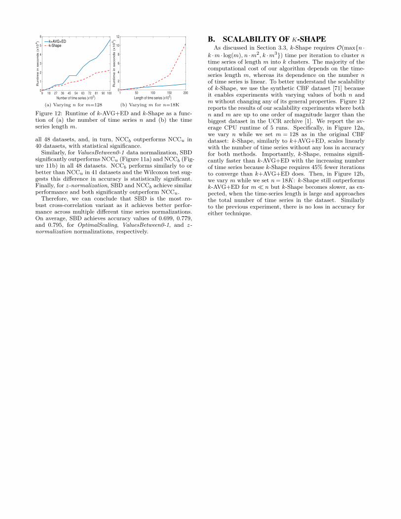
Number of time series (x103)

9 18 27 36 45 54 63 72 81 90 100

Ru

ntim

e in

se

co

nd

s (

x1

04)

0

1

2

3

4

5

6

k+AVG+EDk-Shape

(a) Varying n for m=128Length of time series (x10

2)

1 50 100 150 200

Ru

ntim

e in

se

co

nd

s (

x1

05)

0

2

4

6

8

10

12

(b) Varying m for n=18K

Figure 12: Runtime of k-AVG+ED and k-Shape as a func-tion of (a) the number of time series n and (b) the timeseries length m.

all 48 datasets, and, in turn, NCCb outperforms NCCu in40 datasets, with statistical significance.Similarly, for ValuesBetween0-1 data normalization, SBD

significantly outperforms NCCu (Figure 11a) and NCCb (Fig-ure 11b) in all 48 datasets. NCCb performs similarly to orbetter than NCCu in 41 datasets and the Wilcoxon test sug-gests this difference in accuracy is statistically significant.Finally, for z-normalization, SBD and NCCb achieve similarperformance and both significantly outperform NCCu.Therefore, we can conclude that SBD is the most ro-

bust cross-correlation variant as it achieves better perfor-mance across multiple different time series normalizations.On average, SBD achieves accuracy values of 0.699, 0.779,and 0.795, for OptimalScaling, ValuesBetween0-1, and z-normalization normalizations, respectively.

B. SCALABILITY OF K-SHAPEAs discussed in Section 3.3, k-Shape requires O(max{n ·

k ·m · log(m), n ·m2, k ·m3}) time per iteration to cluster ntime series of length m into k clusters. The majority of thecomputational cost of our algorithm depends on the time-series length m, whereas its dependence on the number nof time series is linear. To better understand the scalabilityof k-Shape, we use the synthetic CBF dataset [71] becauseit enables experiments with varying values of both n andm without changing any of its general properties. Figure 12reports the results of our scalability experiments where bothn and m are up to one order of magnitude larger than thebiggest dataset in the UCR archive [1]. We report the av-erage CPU runtime of 5 runs. Specifically, in Figure 12a,we vary n while we set m = 128 as in the original CBFdataset: k-Shape, similarly to k+AVG+ED, scales linearlywith the number of time series without any loss in accuracyfor both methods. Importantly, k-Shape, remains signifi-cantly faster than k-AVG+ED with the increasing numberof time series because k-Shape requires 45% fewer iterationsto converge than k+AVG+ED does. Then, in Figure 12b,we vary m while we set n= 18K: k-Shape still outperformsk-AVG+ED for m� n but k-Shape becomes slower, as ex-pected, when the time-series length is large and approachesthe total number of time series in the dataset. Similarlyto the previous experiment, there is no loss in accuracy foreither technique.