ADVANCED AIR DATA SENSING TECHNIQUES

Rodney K. Bogue and Lannie D, Webb NASA Flight Research Center

Edwards, California USA

Presented at 5th International Aerospace Instrumentation Symposium

Cranfield, England March 25-28, 1968

https://ntrs.nasa.gov/search.jsp?R=19680027854 2018-07-11T03:05:30+00:00Z

ADVANCED AIR DATA SENSING TECHNIQUES

Rodney K. Bogue and Lannie D. Webb NASA Flight Research Center

INTR ODUC TION

Measurements of total air temperature on research aircraft flying at supersonic and hypersonic speeds are needed for analysis of flight data. Two types of total- temperature sensors--a resistance thermometer (ref. 1) and a shielded thermocouple (ref. +-have been flown on research aircraft by the National Aeronautics and Space Administrationes Flight Research Center at Edwards, California. Total-temperature measurements made by both types of probes are subject to the following basic errors: (1) conduction, (2) radiation, and (3) recovery factor uncertainty. A s the flight testing of research aircraft has progressed to higher Mach numbers, these basic errors in kotal-temperature measurements have also grown larger (ref. 3). Furthermore, the structural integrity of both types of probes becomes marginal as Mach numbers above 5 a re attained in atmospheric flight, In an attempt to reduce the measurement errors in total temperature at Mach numbers greater than 1 and to improve the structural integrity of sensors at high Mach numbers, other less conventional total-temperature sensors are being investigated.

A fluidic (air) oscillator temperature sensor, developed by the U. S. Army's Harry Diamond Laboratories (refs. 4 and 5) and by Honeywell he. (Minneapolis, Minn. ) 9

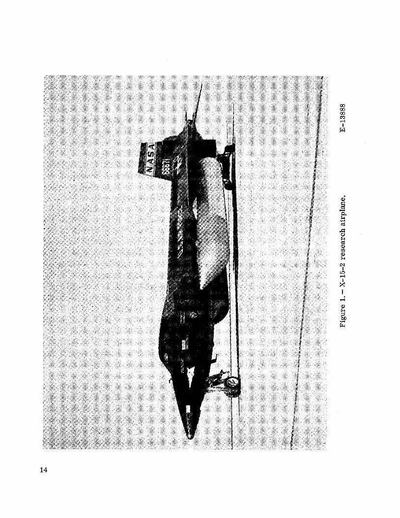
showed promise of high accuracy and structural integrity at stagnation temperatures in excess of 3000" R. Several fluidic total-temperature sensors were built by Honeywell Inc. for the NASA Ames Research Center to be used in wind-tunnel tests as hypersonic boundary-layer probes (ref. 6). Wind-tunnel tests in the Ames 3.5-foot hypersonic tunnel validated the basic concept of the probe operation. A final version of these probes (model C) was loaned ta the Flight Research Center for in-flight eval- uation on the X-15 aircraft (see ref. 7 and fig, 1).

Before flight testing was started, the probe was evaluated at some of the environ- mental conditions that would be encountered during an X-15 flight. Next, the fluidic probe together with a Rosemount 103U triple-shielded thermocouple probe (ref. 8) for comparison, were mounted on the upper vertical fin of the X-15 airplane, For the flight evaluation, special flight signal conditioning and cooling equipment was in- stalled on the airplane.

The fluidic and shielded thermocouple total-temperature probes were flown to a Mach number of 6.70 on flight 53 (October 3, 1967) of the number 2 X-15 airplane. This paper presents details of the installation of the total-temperature probes, flight testing procedures, and results from the X-15 flight.

FLUIDIC SENSOR THEORY

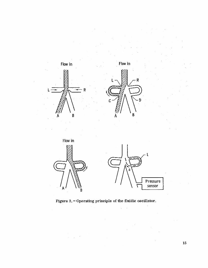
Although the exact internal geometry of the fluidic sensor is classified, its prin- ciple of operation may be described with a simple model. The oscillator is an adap- tation of a bistable fluid amplifier (fig. 2(a)). The tendency of the fluid stream to attach itself to a nearby wall (commonly termed the Coanda effect) forms the basis of operation. The flow will continue in leg A until sufficient flow is introduced into the adjacent control port (L) to cause the flow to detach from the wall and attach to the opposite wall, causing a flow in leg B (not shown). An oscillator may be constructed by taking some of the out- put flow of the amplifier and returning it to the control ports (fig. 2(b)). Part of the flow in leg A is diverted through port C around the feedback path into control port L. This diversion causes the flow to switch from leg A to leg B (fig. 2(c)). The resulting di- version from leg B through port D around the feedback path to control port R causes the flow to switch from leg B back to leg A where the cycle repeats itself.

The period (t) of this oscillation is dependent upon both the length of the feedback path (2 ) and the velocity of propagation of the pressure pulse (a) along the feedback path (fig. 2(d)) as shown in the equation

t = - 21 a

In an ideal gas, the velocity of propagation is related to the absolute temperature by the equation

a=J rRT (2)

The frequency of oscillation then becomes

where k is dependent upon the feedback path length and the gas parameters, as

k = q (4)

If the feedback path length is invariant and if y and R do not change, the frequency is then a function only of the absolute temperature to the one-half power. Or, con- versely, the equation for temperature measurement as a function of frequency becomes

1 2 T -- - (k)2 (5)

For high-temperature applications, the factor k is, itself, a function of temperature. The ratio of gas specific heats (7) changes, becoming less as the temperature is in- creased and the feedback path length increases as a result of the thermal expansion of the oscillator body. The following equation was empirically derived by Honeywell Inc. from laboratory tests :

Tf = 3.7293 X 10-7f2* 0855 (6)

2

This equation provides an approximate correction for the variable k by increasing the exponent on the frequency from 2 to 2.0855.

The addition of a pressure sensor to one output leg of the basic fluidic oscillator permits the pressure fluctuations to be sensed externally (fig. 2(d)).

DESCRIPTION OF APPARATUS

Fluidic To tal- Temperature Sensor

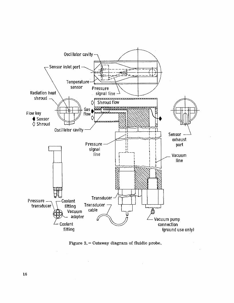
The fluidic total-temperature probe designed by Honeywell for the Ames Research Center is illustrated in figure 3. Hot stagnation air enters the sensor through the sen- sor inlet port and passes through the oscillator. After leaving the oscillator area, the air is channeled rearward and is exhausted from the sensor exhaust port. (The dark arrow in the figure illustrates the air flow through the sensor.) The pressure fluctu- ations (frequency) from the oscillator are propagated through the pressure signal line to the transducer. Here, the pressure signal is converted to an electrical signal for recording or telemetry purposes, or both. A piezoelectric-type pressure transducer was selected for use in the fluidic sensor. Good high-frequency response and relative insensitivity to high temperatures were the primary reasons for this selection.

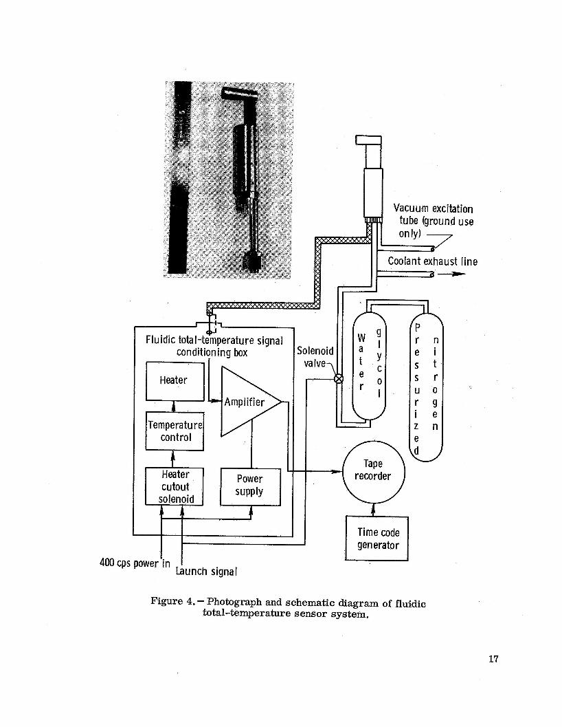
Figure 4 shows the sensor and the required signal conditioning and recording equip- ment needed for data gathering. Both absolute inlet pressure and differential pressure across the probe influence the probe characteristics. These effects are reflected pri- marily in the amplitude of the pressure fluctuation produced by the oscillator. In order to minimize the effect of downstream pressure, the flow exhaust is maintained at a pressure sufficiently low to cause sonic flow downstream from the oscillator section. This choked condition causes the pressure sensitivity to be a fqnction only of the abso- lute inlet pressure. Empirical adjustment of critical sensor dimensions produced a unit with a frequency output that was nearly insensitive to inlet pressure variations over a limited pressure range.

The requirement for choked flow inside the probe limits the application of this unit to supersonic flight speeds unless a vacuum pump is provided. In the X-15 application, choked flow was maintained from slightly after launch until the subsonic condition was reached just prior to landing.

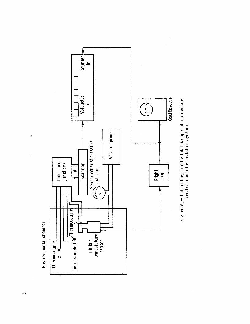
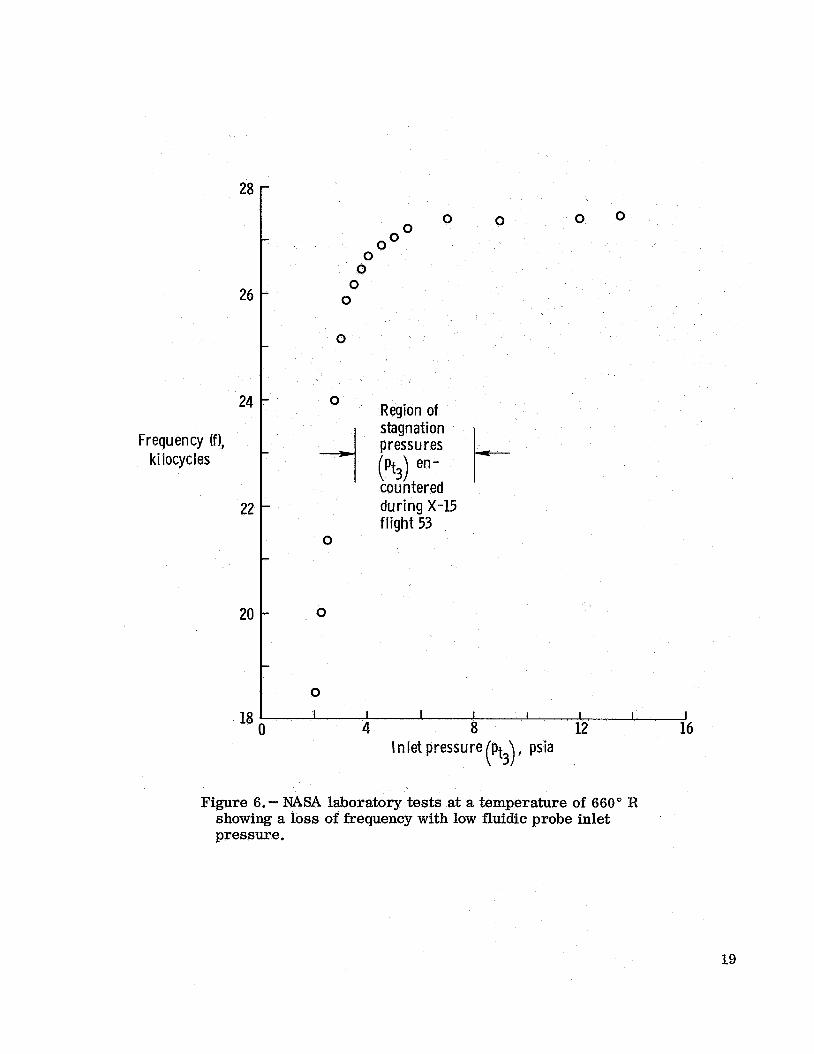
A laboratory calibration check was performed on the fluidic probe prior to instal- lation on the X-15 aircraft. The purpose of this check was two-fold: first, to verify a point on the temperature versus frequency calibration curve, and, second, to investi- gate the effects of low inlet pressures. Figure 5 shows the laboratory system. Lab- oratory test data shown in figure 6 illustrate the output frequency variation for constant temperature as a function of absolute inlet pressure.

Shielded Total-Temperature Sensor

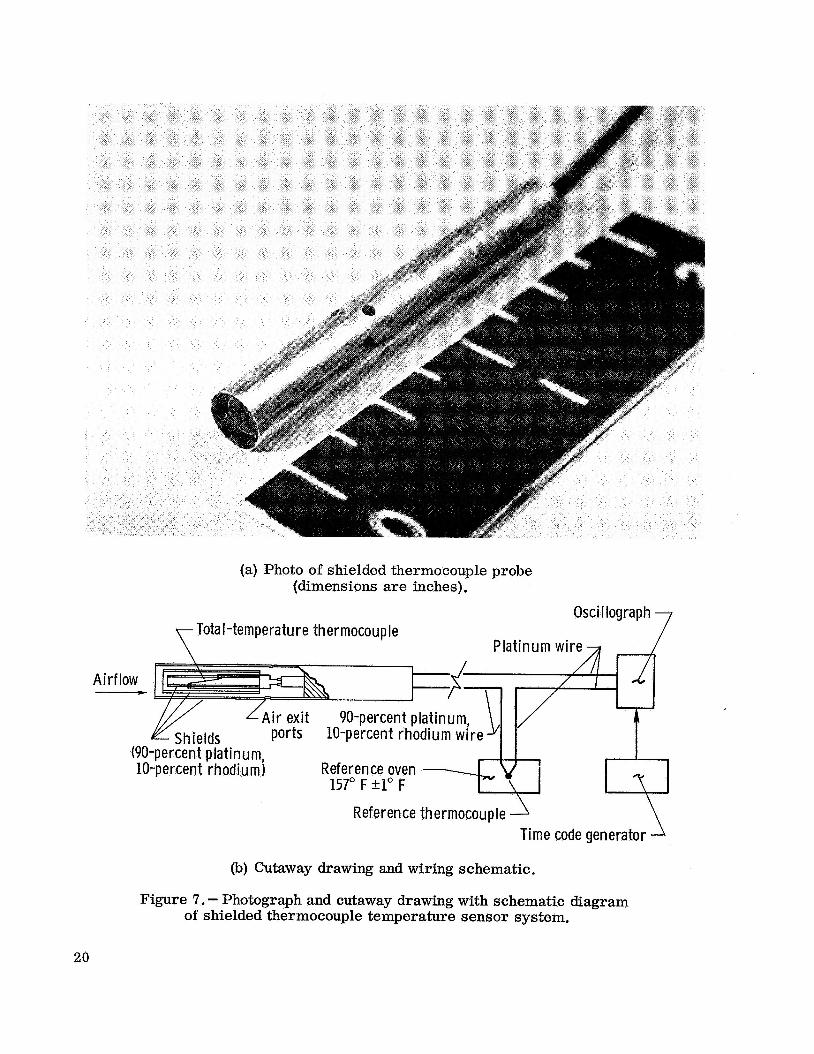
The conventional thermocouple total-temperature sensor used in the flight system was a commercially available Type 103U manufactured by the Rosemount Engineering Company. This sensor uses a platinum/platinum-lQ-percent rhodium thermocouple

3

which is heated by conduction from the stagnation air to a recovery temperature that closely approximates the true total temperature. The radiation shields and support are designed to reduce the loss of heat by conduction and radiation. To replenish some of the energy lost through conduction and radiation from the thermocouple junction to the walls, a flow of air is allowed through small vent holes in the outer shield (ref. 9). De- tails of this sensor a re included in reference 8. Figure 7 illustrates the sensor con- figuration and the associated data-gathering system that was used for the X-15 flight.

Total- Temperature -Pr obe Support Equipment

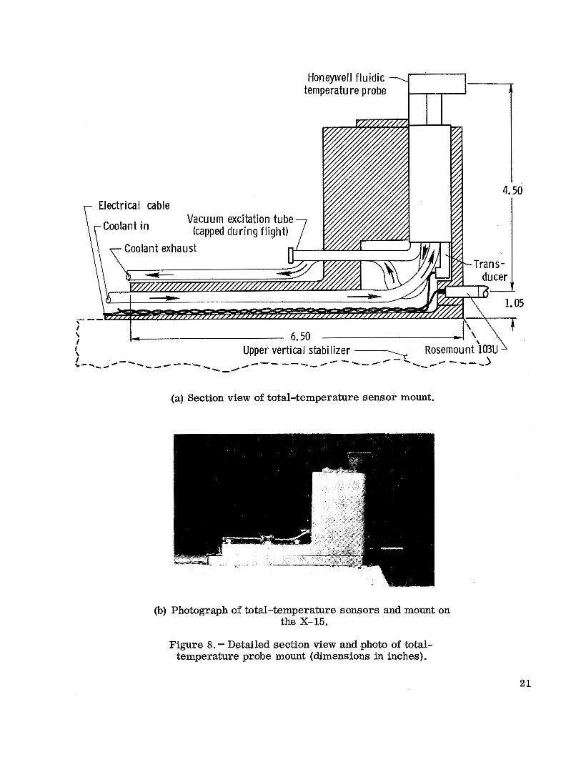
X-15 sensor mount.- The sensor mount was designed to accommodate, in prox- imity, both the fluidic sensor and the conventional sensor (figs. 8 to 10). Provision was made for electrical signal leads and the coolant tubing to be routed to the sensors. An external connection from the probe exhaust was provided to permit ground stimu- lation of the fluidic sensor (figs. 4 and 8). This connection was sealed for flight oper- ation.

Cooling equipment. - The cooling required by the piezoelectric pressure transducer was supplied by a pressurized water-glycol system (ref. 10). The water-glycol coolant flowed through the system under pressure from compressed nitrogen. This system was not actuated until launch. At this time a solenoid valve was opened, allowing the coolant to flow from the reservoir tank through the base of the fluidic sensor and out the exhaust port. Figure 11 illustrates the cooling-tank configuration mounted on the base of the X-15 vertical stabilizer. Figure 4 shows the cooling system schematically.

Signal conditioning equipment. - Signal conditioning equipment for the fluidic sensor was limited to a band-pass amplifier with a high-impedance input. The amplifier cir- cuitry was developed by Honesel l Inc. for use with-the wind-&el system. The air- borne application required that the circuitry be packaged to withstand shocks and accel- erations experienced in flight. Integral electrical heaters were also needed to assure amplifier operation in the -60" F environment prior to X-15 launch. This amplifier, with a voltage gain of 85 decibels from 18 to 63 kilocycles, was used to provide a signal of sufficient amplitude for recording on the on-board tape recorder.

The thermocouple reference junction oven provided a reference junction at 157" F for the Rosemount 103U sensor. This signal with no further amplification was used to drive the on-board oscillographic recording equipment.

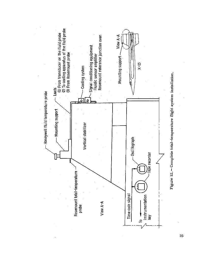
Figure 11 shows the amplifier and the reference junction oven mounted on the base of the X-15 vertical stabilizer. Figures 4 and 7 show schematically the location of both the amplifier and the reference junction oven in their respective systems. Figure 12 illustrates the general locations of the various system components.

FLIGHT DATA -REDUCTION PROCEDURE

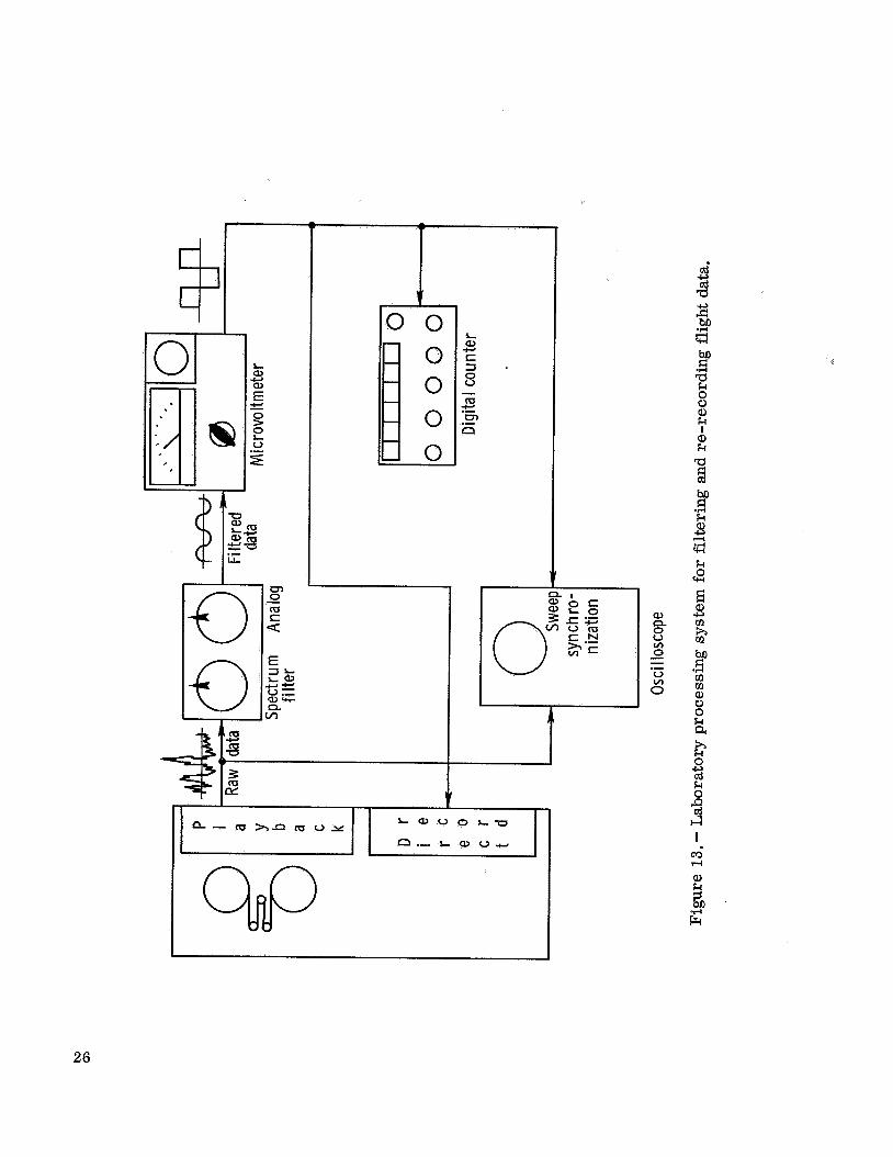
The fluidic sensor signal was recorded with an airborne tape recorder, A duplicate tape was prepared from the flight tape and was used throughout the remainder of the data-processing sequence. Figure 13 illustrates the system used during the first step in the data-processing sequence, Raw data from the tape were first filtered by the

4

spectrum analog filter to reduce the noise present. Af te r being filtered, the signal was processed by the microvoltmeter. This unit, working on the phase lock loop principle, was designed to measure single frequency signals in the presence of large amounts of noise, An internal feedback system is used that phase locks an internal oscillator to the same frequency as the input signal. This oscillator signal output provides a replica of the input signal without the attendant noise and amplitude variations of the raw data.

The signal from the microvoltmeter was used to drive a direct record amplifier on the same tape unit that was providing the raw data from a playback amplifier. With this arrangement the signal was played back, processed, and re-recorded on a parallel tape channel with the raw data. Time correlation was maintained by the time code signal also on the tape.

The operation of this system required that both the spectrum analog filter and the microvoltmeter be continuously adjusted during the playback of the data. The filter was adjusted to maintain the signal frequency within the band pass, The microvoltmeter was adjusted to maintain the signal lock condition. A frequency dial must be set within 5 percent of the signal frequency for the unit to capture and lock on the signal. Adjust- ment of the controls on both units are made by referring to the frequency counter being driven by the output of the microvoltmeter.

An oscilloscope connected for viewing the raw data was used to verify the signal lock state of the microvoltmeter. The sweep generator on the oscilloscope was syn- chronized with the microvoltmeter output. As long as the signal lock condition existed, a stationary pattern was displayed on the scope. When signal lock was lost, the sta- tionary display became erratic.

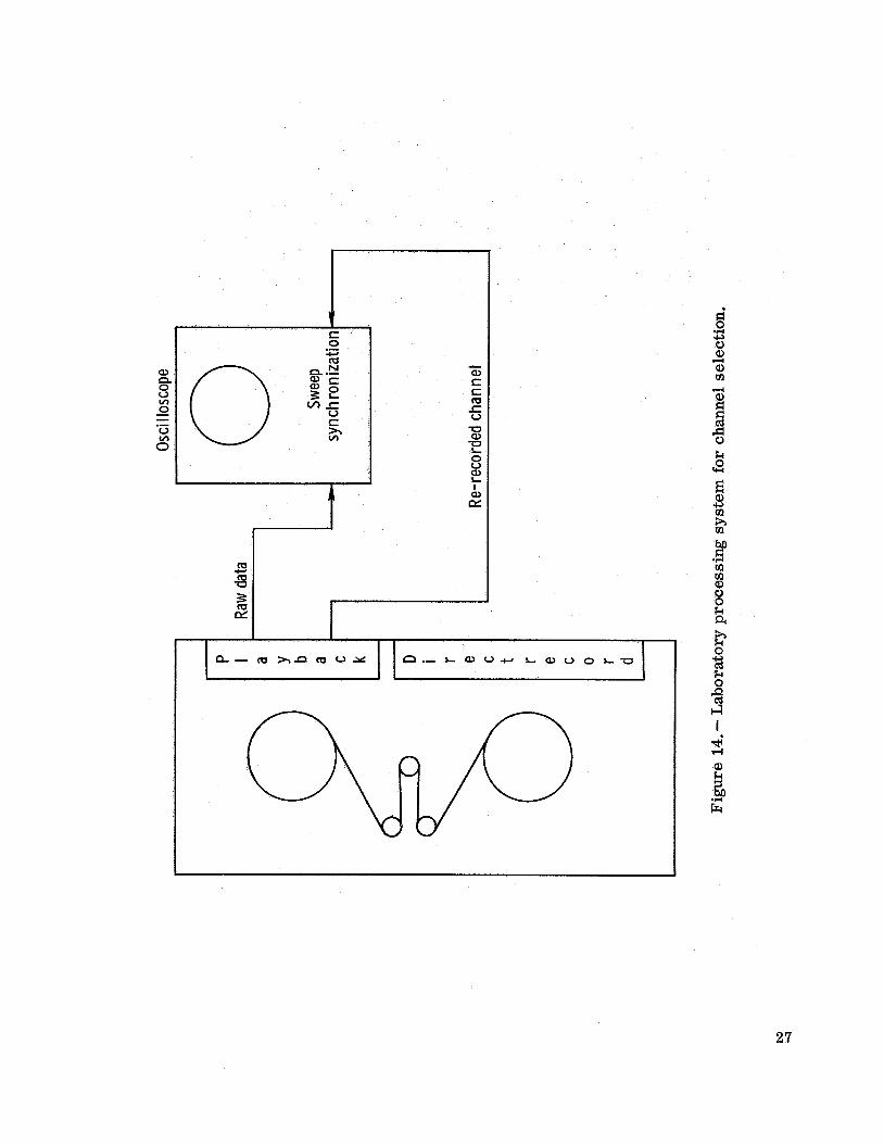
Because of the numerous adjustments required during each data-processing sequence, occasionally the signal was momentarily lost because of a faulty setting on either the filter o r the microvoltmeter. For this reason, the data-processing sequ.ence was re- peated once for each spare tape channel. Ten of the 14 channels were available, and the sequence was repeated for each channel. A selection was then made of the channel that had the least number of signal dropouts. The procedure used to select this channel was similar to that used to verify the signal lock condition on the microvoltmeter. This time, the signal from the tape channel being inspected was used to synchronize the sweep generator on the oscilloscope (fig. 14). A s before, a stationary display indicated good tracking, and a nonstationary display revealed a frequency mismatch. The channel deemed most representative was used for the succeeding data processing.

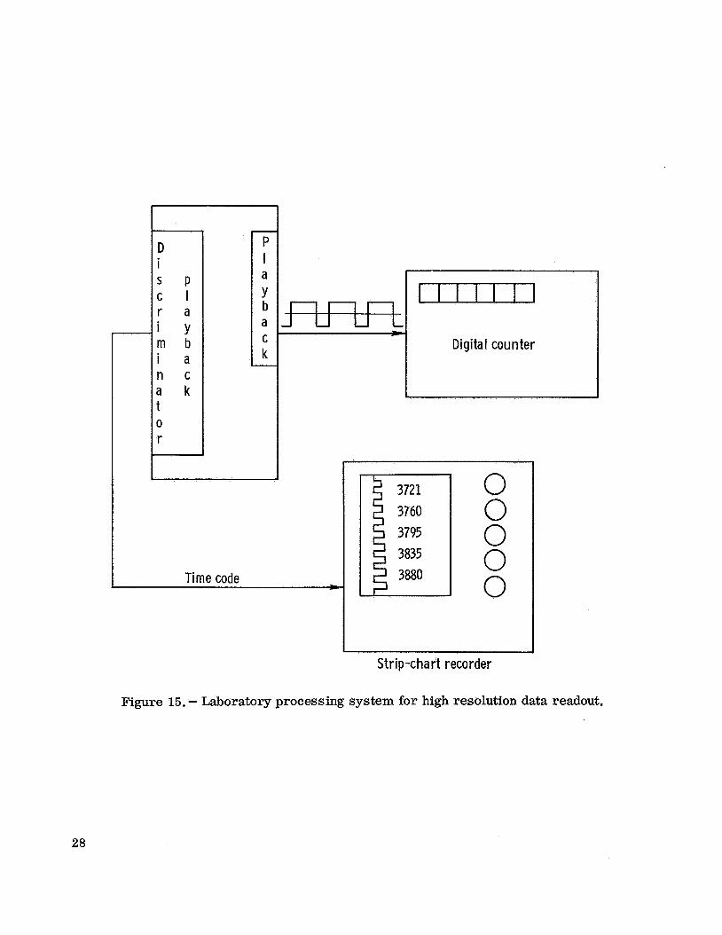
A frequency time history of the flight was obtained by playing back the re-recorded signal into a frequency counter and manually recording the counter indicated frequency information for each second of flight (fig. 15). Time correlation was accomplished by recording the tape time code on the strip chart recorder and manually writing the frequency values directly on the strip chart at 1-second intervals. The tape was run at a reduced speed from real time to allow time for manual data recording.

The time code signal recorded both on the flight oscillograph film and the flight tape permitted the shielded thermocouple temperatures to be correlated with the tem- peratures from the fluidic sensor.

5

RESULTS AND DISCUSSION

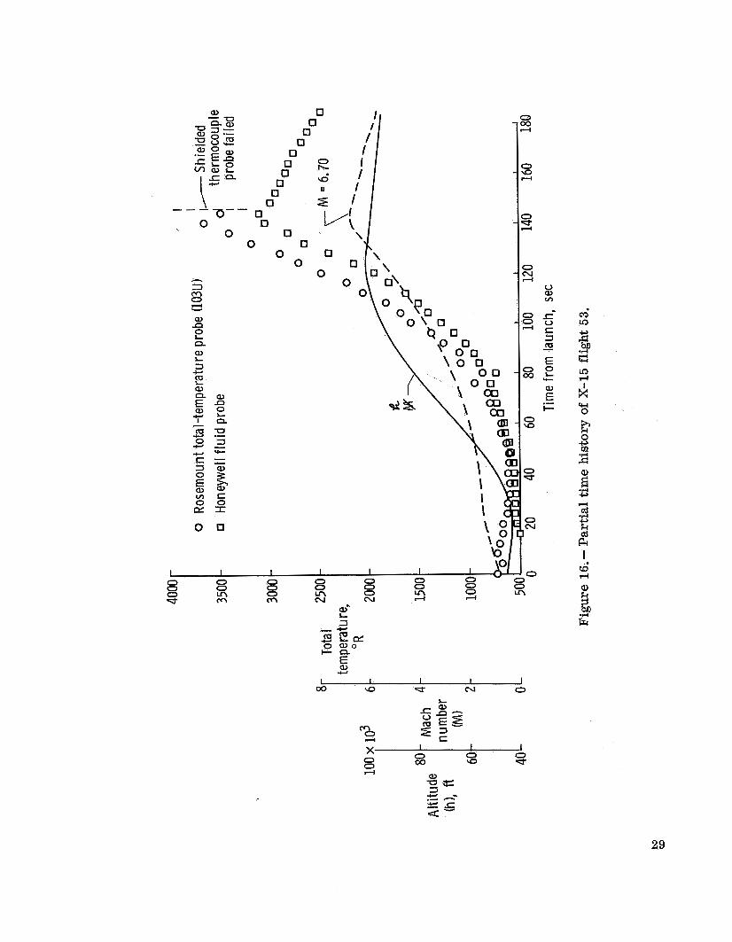
Figure 16 is a partial total-temperature time history of X-15 flight 53 up to peak Mach number. Radar measurements (converted to free stream) of the X-15 Mach num- ber and altitude (ref. 11) are shown in addition to the data obtained from the shielded thermocouple sensor and the fluidic sensor. In figure 16, the total temperature mea- sured by the fluidic probe was calculated by using equation (6). As indicated in the fig- ure, the shielded thermocouple probe failed a short time after peak Mach number was attained. Figure 17 shows the variation of ambient temperature with altitude, obtained just prior to flight from radiosonde measurements, which was used to analyze the flight data,

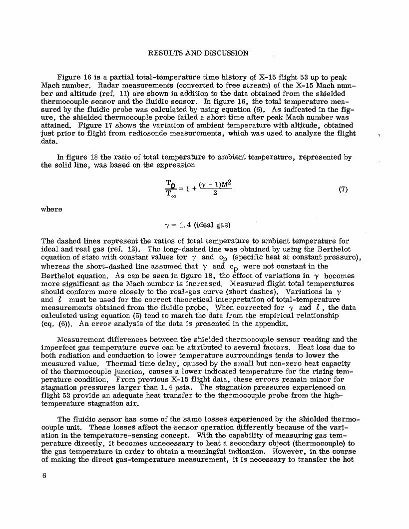
In figure 18 the ratio of total temperature to ambient temperature, represented by the solid line, was based on the expression

( y - 1)M2 T* x = 1 + TKI

where

y = 1 . 4 (ideal gas)

The dashed lines represent the ratios of total temperature to ambient temperature for ideal and real gas (ref. 12). The long-dashed line was obtained by u.sing the Berthelot equation of state with constant values for y and cp (specific heat at constant pressure), whereas the short-dashed line assumed that y and cp were not constant in the Berthelot equation. A s can be seen in figure 18, the effect of variations in y becomes more significant as the Mach number is increased, Measured flight total temperatures should conform more closely to the real-gas curve (short dashes). Variations in y and 1 must be used for the correct theoretical interpretation of total-temperature measurements obtained from the fluidic probe. When corrected for y and I , the data calculated using equation (5) tend to match the data from the empirical relationship (eq. (6)). An error analysis of the data is presented in the appendix.

Measurement differences between the shielded thermocouple sensor reading and the imperfect gas temperature curve can be attributed to several factors. Heat loss due to both radiation and conduction to lower temperature surroundings tends to lower the measured value. Thermal time delay, caused by the small but non-zero heat capacity of the thermocouple junction, causes a lower indicated temperature for the rising tem- perature condition. From previous X-15 flight data, these errors remain minor for stagnation pressures larger than 1.4 psia. The stagnation pressures experienced on flight 53 provide an adequate heat transfer to the thermocouple probe from the high- temperature stagnation air.

The fluidic sensor has some of the same losses experienced by the shielded thermo- couple unit. These losses affect the sensor operation differently because of the vari- ation in the temperature-sensing concept. With the capability of measuring gas tem- perature directly, it becomes unnecessary to heat a secondary object (thermocouple) to the gas temperature in order to obtain a meaningful indication. However, in the course of making the direct gas-temperature measurement, it is necessary to transfer the hot

6

gas into the fluidic oscillator. During this transfer, heat is conducted from the gas to the cooler cavity and surrounding support structure, thus reducing the gas temperature. The temperature actually measured is an average value of the gas within the oscillator cavity, o r the real-gas total temperature reduced by the conduction losses.

The fluidic temperature sensor calibration curve is a possible source of additional errors, It was not possible to verify the high-temperature portion of the curve before flight, This section of the calibration curve was obtained by extrapolating lower tem- perature data.

No attempt was made during the first flight to measure the oscillator body temper- ature. Had this information been available, an approximation could have been generated that would account far the heat loss to the oscillator body and the change in the feedback path length.

Additional errors may arise i f the inlet stagnation pressures of the fluidic sensor drop below 5 psia. All wind-tunnel tests have been performed at stagnation pressures of 600 psi o r greater (ref. 6). Laboratory experiments by Honeywell Inc. and the NASA Flight Research Center have indicated that a reduction in frequency may result i f stag- nation pressures fall below 5 psi (fig. 6) for the Type C fluidic temperature sensor. This pressure effect may be a consequence of the noisy signal output that occurs at low inlet pressures. The digital counter that was used to measure the laboratory data requires a relatively clean input signal for proper operation. It is suspected that the noisy data signal was not sufficiently defined at the low inlet pres- sures to provide a reliable trigger signal to the digital counter. The microvoltmeter is capable of detecting the signal in the high background noise and providing a clean square-wave signal output of the same frequency as the input signal. Further laboratory tests with the microvoltmeter are expected to resolve this question. The microvoltmeter was not available when the preflight tests were made but was utilized for the flight data processing.

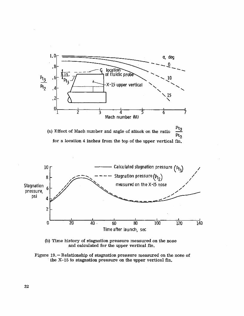
The magnitudes of inlet stagnation pressures encountered during flight 53 were estimated from previous measurements made near the top of the upper vertical fin. Figure 19(a) shows the relationship between the stagnation pressures on the upper ver- tical tail (ptg) and the stagnation pressures measured on the nose @t,) of the X-15.

After adjustment for angle of attack (a) , stagnation pressures on the upper vertical fin (solid line, fig. 19(b)) fell below 5 psia during portions of the X-15 flight. The pos- sible effects of the low inlet pressures on the recorded frequency from the fluidic probe are shown in figure 6. Further laboratory tests are expected to provide a basis for a possible pressure correction to the flight data.

The increase in the gas viscosity as higher temperatures are attained may cause a signal attenuation in addition to that resulting from the reduced inlet stagnation pressure. This effect would tend to reduce the signal-to-noise ratio for high-temperature operation.

CONCLUDING REMARKS

This investigation has established the feasibility of using a fluidic-type temperature sensor for measuring total temperature on an aircraft traveling at hypersonic speeds within the atmosphere. Also, problem areas that do not severely limit the application

7

but that do require further study to assess the total effect of each problem on the system operation have been revealed.

Further flight testing of fluidic sensors to determine the cause of the lower indi- cated total temperatures is needed. This future work should include measurements of stagnation pressure, base pressure, and oscillator body temperature. In addition, ex- tensive laboratory tests should be made with improved equipment to assess individually the effects of these parameters on sensor operation. It is hoped that these measurements and the subsequent data reduction and study will make it possible to significantly in- crease the accuracy and reliability of the fluidic temperature sensor and that this effort will contribute to the overall understanding of fluidic temperature sensors.

An improved sensor specifically designed for flight operation is being built under contract by the Honeywell Systems and Research Division. This unit is being optimized for low-pressure operation and will include a means for measuring oscillator body tem- perature.

8

APPENDIX

ERROR ANALYSIS

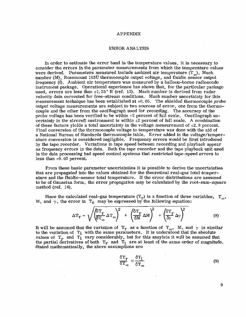
In order to estimate the error band in the temperature values, it is necessary to consider the errors in the parameter measurements from which the temperature values were derived. Parameters measured include ambient a i r temperature (T,) , Mach number (M), Rosemount 103U thermocouple output voltage, and fluidic sensor output frequency (f). Ambient air temperature was measured by a balloon-borne radiosonde instrument package. Operational experience has shown that, for the particular package used, e r rors are less than kl. 25" R (ref. 13). Mach number is derived from radar velocity data corrected for free-stream conditions. Mach number uncertainty for this measurement technique has been established at -10. 05. The shielded thermocouple probe output voltage measurements are subject to two sources of error , one from the thermo- couple and the other from the oscillograph used for recording. The accuracy of the probe voltage has been verified to be within -12 percent of full scale, Oscillograph un- certainty in the aircraft environment is within k2 percent of full scale. A combination of these factors yields a total uncertainty in the voltage measurement of k2.8 percent. Final conversion of the thermocouple voltage to temperature was done with the aid of a National Bureau of Standards thermocouple table. Error added in the voltage/temper- ature conversion is considered negligible. Frequency errors would be first introduced by the tape recorder. Variations in tape speed between recording and playback appear as frequency errors in the data. Both the tape recorder and the tape playback unit used in the data processing had speed control systems that restricted tape-speed errors to less than 1t0.02 percent.

From these basic parameter uncertainties it is possible to derive the uncertainties that a re propagated into the values obtained for the theoretical real-gas total temper- ature and the fluidic-sensor total temperature. If the e r ror distributions are assumed to be of Gaussian form, the error propagation may be calculated by the root-sum-square method (ref. 14).

Since the calculated real-gas temperature (Tr) is a function of three variables, T,, M, and y, the e r ror in Tr may be expressed by the following equation:

It will be assumed that the variation of Tr as a function of T,, M, and y is similar to the variation of Ti with the same parameters. It is understood that the absolute values of T the partial drerivatives of both Tr and Ti are at least of the same order of magnitude. Stated mathematically, the above assumptions a re

and Ti vary considerably, but for this anaylsis it will be assumed that

9

6Tr 6Ti -e- 6M - 6M

and

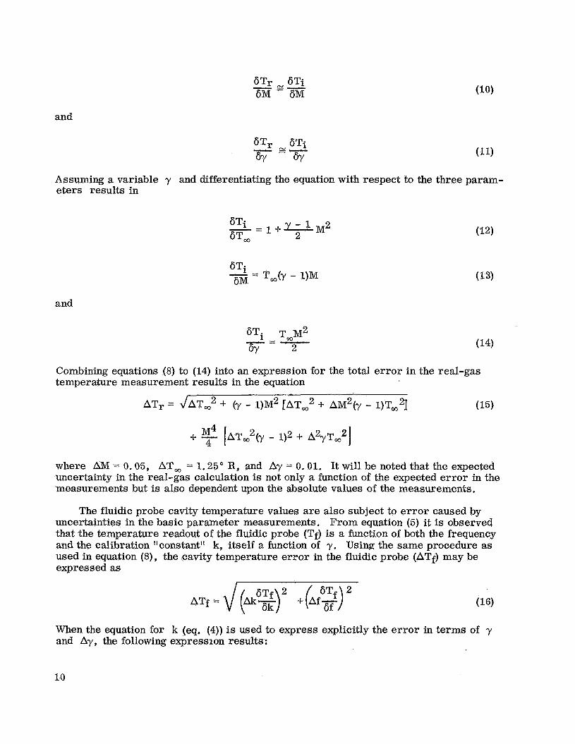
Assuming a variable y and differentiating the equation with respect to the three param- eters results in

and

Combining equations (8) to (14) into an expression for the total error in the real-gas temperature measurement results in the equation

ATr = JATW2 + (7 - 1)M2 [ATW2 + AM2(y - 1)TW2] (15)

-t- [ATW2(y - 1)2 f A2yTw2] 4

where AM = 0.05, AT, = 1.25" R , and Ay = 0.01. It will be noted that the expected uncertainty in the real-gas calculation is not only a function of the expected error in the measurements but is also dependent upon the absolute values of the measurements.

The fluidic probe cavity temperature values are also subject to e r ror caused by uncertainties in the basic parameter measurements. From equation (5) it is observed that the temperature readout of the fluidic probe (Tf) is a function of both the frequency and the calibration "constant" k, itself a function of y. Using the same procedure as used in equation (S), the cavity temperature error in the fluidic probe (ATf) may be expressed as

When the equation for k (eq. (4)) is used to express explicitly the e r ror in terms of y and Ay, the following expression results:

10

ATf =% d(F)2 + (hf) 2

where Af = 120 cycles/second.

Predicted e r ror bands for the three temperature measurements at a Mach number of 6.70 are

ATs. = *95" R

ATr = *loo" R

and

ATf = ~ 2 5 " R

It should be pointed out that the predicted error of the fluidic probe is, in reality, the e r ror in the cavity temperature measurement not the total-temperature measurement.

11

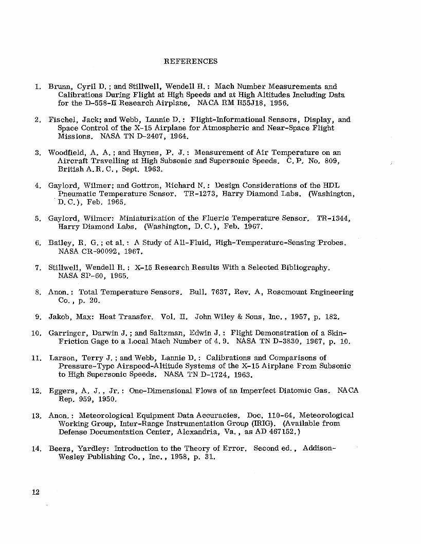
REFERENCES

1.

2.

3.

4.

5.

6.

7.

8.

9.

10.

11.

12.

13.

14.

Brunn, Cyril D. ; and Stillwell, Wendell H. : Mach Number Measurements and Calibrations During Flight at High Speeds and at High Altitudes Including Data for the D-558-II Research Airplane, NACA RM H55J18, 1956.

Fischel, Jack; and Webb, Lannie D. : Flight-Informational Sensors, Display, and Space Control of the X-15 Airplane for Atmospheric and Near-Space Flight Missions. NASA TN D-2407, 1964.

Woodfield, A. A. ; and Haynes, P. J. : Measurement of A i r Temperature on an Aircraft Travelling at High Subsonic and Supersonic Speeds. C, P. No. 809, British A. R. C. , Sept. 1963.

Gaylord, Wilmer; and Gottron, Richard N. : Design Considerations of the HDL Pneumatic Temperature Sensor. TR-1273, Harry Diamond Labs. (Washington, D. C.) , Feb. 1965.

Gaylord, Wilmer: Miniaturization of the Flueric Temperature Sensor. TR-1344, Harry Diamond Labs. (Washington, D. C. ), Feb. 1967.

Bailey, R. G. ; et al. : A Study of All-Fluid, High-Temperature-Sensing Probes. NASA CR-90092, 1967.

Stillwell, Wendell H. : X-15 Research Results With a Selected Bibliography. NASA SP-60, 1965.

Anon. : Total Temperature Sensors. Bull. 7637, Rev. A , Rosemount Engineering Go., p. 20.

Jakob, Max: Heat Transfer. Vol. II. John Wiley 8~ Sons, InC. , 1957, p. 182.

Garringer, Darwin J. ; and Saltzman, Edwin J. : Flight Demonstration of a Skin- Friction Gage to a Local Mach Number of 4.9. NASA TN D-3830, 1967, p. 10.

Larson, Terry J. ; and Webb, Lannie D. : Calibrations and Comparisons of Pressure-Type Airspeed-Altitude Systems of the X-15 Airplane From Subsonic to High Supersonic Speeds. NASA TN D-1724, 1963.

Eggers, A. J. , Jr. : One-Dimensional Flows of an Imperfect Diatomic Gas. NACA Rep. 959, 1950.

Anon. : Meteorological Equipment Data Accuracies. Doc. 110-64, Meteorological Working Group, Inter-Range Instrumentation Group (IRIG). (Available from Defense Documentation Center, Alexandria, Va. , as AD 467152.)

Beers, Yardley: Introduction to the Theory of Error. Second ed. , Addison- Wesley Publishing Co., Inc., 1958, p. 31.

12

a

cP f

h

k

1

M

P

R

T

t

a

Y

A

6

SYMBOLS

velocity of propagation

specific heat at constant pressure

frequency

geometric altitude

fluidic-sensor coefficient

feedback path length

Mach number

pressure

universal gas constant

temperature

period of oscillation

angle of attack

ratio of gas specific heats

incremental error

partial differential

Subscripts:

f fluidic-sensor measurement

i ideal gas

0 total or stagnation conditions

r real gas

st shielded-thermocouple measurement

t2

t3

W static or ambient conditions

stagnation pressure on nose of X-15

stagnation pressure near top of upper vertical stabilizer

13

6 k cd a, m Q) k

14

Flow in

L R

A B

Flaw in

Flow in

2.

Pressure T- sensor

Figure 2. - Operating principle of the fluidic oscillator.

15

fitting (ground use only)

Figure 3. - Cutaway diagram of fluidic probe.

16

Vacuum excitation tube (wound use

117 88 I I Coolant exhaust l ine

-.IF=-- +

Heater G Tempera t u re

control

Amplif ier c7' Solenoid

va Ive,

It------ 400 cps power 'in I

Launch signal

recorder -0 Time code generator

P r n e i s t s r u o r g i e z n e d u

Figure 4. - Photograph and schematic diagram of fluidic total-temperature sensor system.

17

L a3 n E m c V

m - -I.-

G 2 E S

> I= w

.-

L

L a3 + Q)

E .E

~ P

T

L + I

18

28

26

24

Frequency (f), kilocycles

22

20

18

0 000 0 0 0

0

0

-I

0 0 0 0

Region of stagnation pressures

cou n t er ed (Pt3) en-

dur ing X-15 f l ight 53

0

0

0 I I 1 1 1 1 1 1

4 8 12 16 In le t pressure(pt3), psia

Figure 6. - NASA laboratory tests at a temperature of 660" R showing a loss of frequency with low fluidic probe inlet pres sure.

19

(a) Photo of shielded thermocouple probe (dimensions are inches).

Tota I-temperatu r e thermocouple

Airflow ___)

(90-percen t pla tin um, 10-percent rhodium 1

Reference thermocouple Time code generator

(b) Cutaway drawing and wiring schematic.

Figure 7. - Photograph and cutaway drawing with schematic diagram of shielded thermocouple temperature sensor system.

20

. . .

Hon e y e I I f I u idic temperature probe

4.50 ectricai cable

(a) Section view of total-temperature sensor mount.

(b) Photograph of total-temperature sensors and mount on the X-15.

Figure 8.- Detailed section view and photo of total- temperature probe mount (dimensions in inches).

21

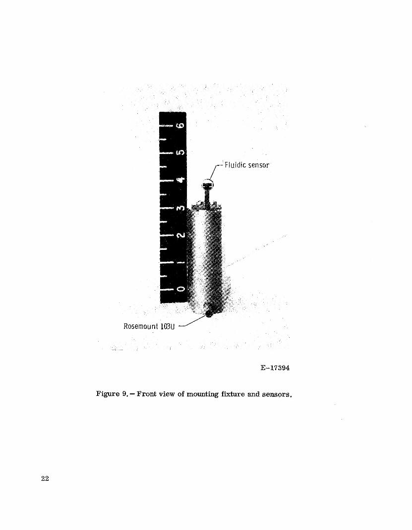
1 R o s ~ ~ ~ u nt 103U

E-17394

Figure 9. - Front view of mounting fixture and sensors,

22

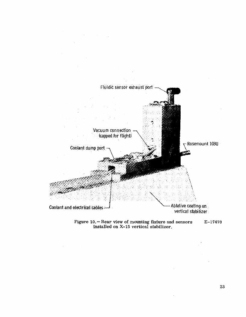
Figure 10.-Rear view of mounting fjxture and sensors E-17470 installed on X- 15 vertical stabilizer.

23

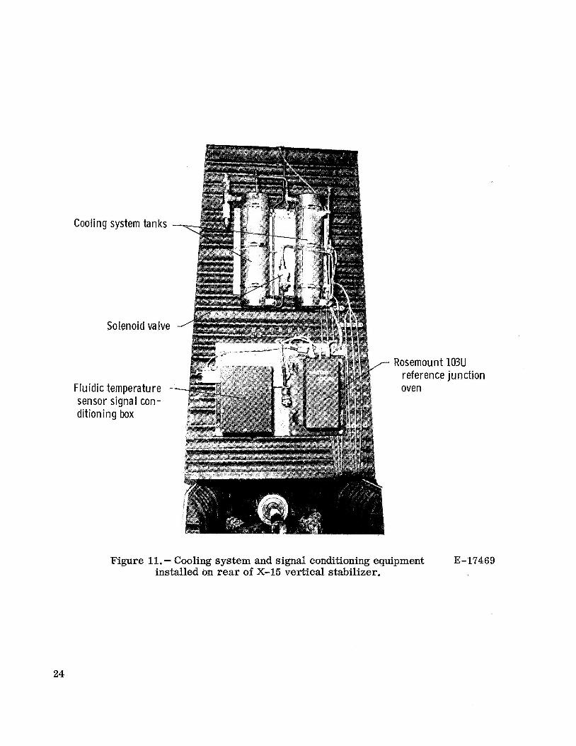
Cooling system tanks

Solenoid valve

Fluidic temperature sensor signa I con - ditioning box

Rosemount 103U reference junct ion oven

Figure 11. - Cooling system and signal conditioning equipment E-17469 installed on rear of X-15 vertical stabilizer.

24

\

P +z 3 > Q) .-

I

25

I

L al i-.

al

2E 0 > V

E

2 .-

I

-0 Q

k 0 %I

a

B a, -c, m

26

b .-

27

D

S P C I r a i Y m b i a n c a k t

r

I

0

a i k C

Time code

1111111 Digital counter

3 3721 3760 3795 3835 3880

0 0 0 0 0

Strip-chart recorder

Figure 15. - Laboratory processing system for high resolution data readout.

28

I I I I I \o U N 0 03

L

29

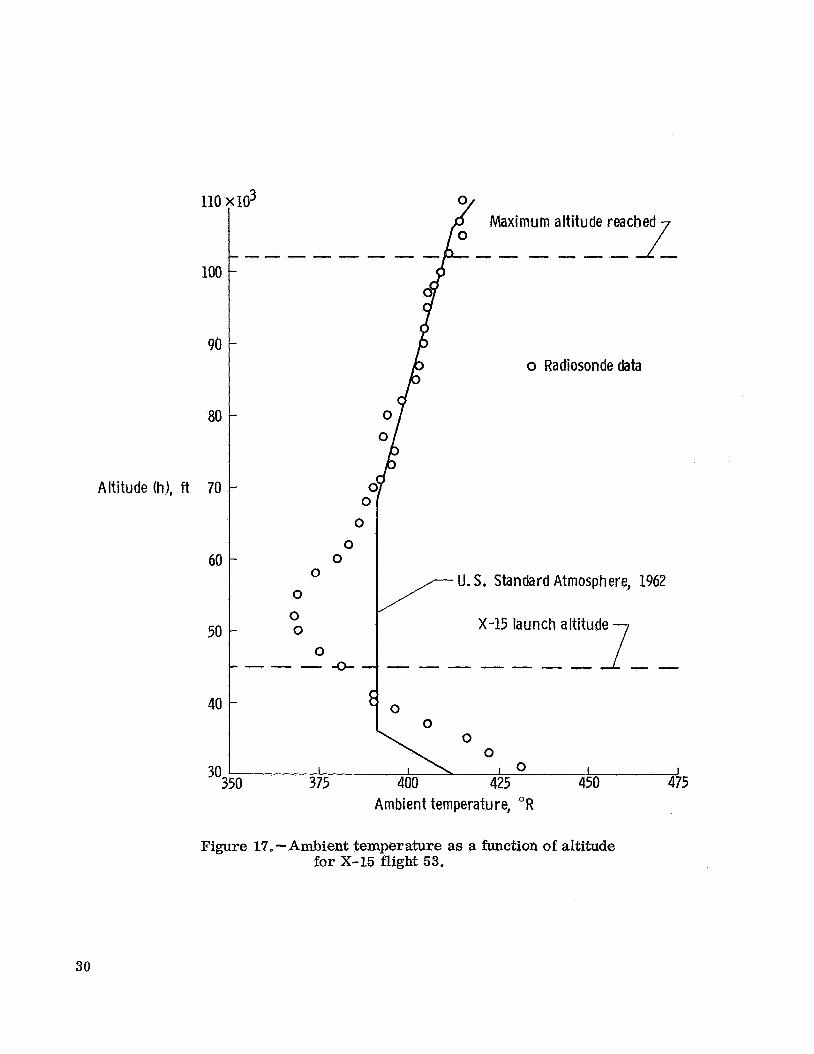
o Radiosonde data

Maximum altitude reached

------

Altitude (h), ft 70

U. S . Standard Atmosphere, 1962

X-15 launch altitude

---

Ambient temperature, O R

Figure 17.-Ambient temperature as a function of altitude for X-15 flight 53.

30

Temperature

10

ratio

Ideal gas

Idea I gas Real gas

-- -----

Measured data

o Rosemount 103U probe o Honeywell f lu id probe

Using Berthelot equation (ref. 12)

Mach number (M)

Figure 18. - Comparison of total-temperatures measured on X-15 flight 53 with real- and ideal-gas curves.

31

Pt2

1.0-

.a-

.6-

.4-

.2-

2 -

-- \ \ \

X-15 upper vertical ', \

I I I I I I I

0 -4r

-\

10 \ \

\ 15 \

I I I I I I 1 2 3 4 5 6 7

Mach number (MI

01

(a) Effect of Mach number and angle of attack on the ratio Pto

Y

for a location 4 inches from the top of the upper vertical fin.

(b) Time history of stagnation pressure measured on the nose and calculated for the upper vertical fin.

Figure 19. - Relationship of stagnation pressure measured on the nose of the X-15 to stagnation pressure on the upper vertical fin.

32