june 5, 2019. - oregon state university
TRANSCRIPT

AN ABSTRACT OF THE THESIS OF
Matthew H. Kremer for the degree of Master of Science in Materials Science presented on
June 5, 2019.
Title: Electrospray Deposition of Discrete Nanoparticles: Studies on Pulsed-Field
Electrospray and Analytical Applications
Abstract approved: ______________________________________________________
Vincent T. Remcho
Electrospinning and electrospray are both nano-scale material fabrication
techniques, based on related phenomena of electrically charged fluid spray from a droplet
of liquid. Material is dissolved in liquid, then a spray is generated by applying a high
voltage, creating an electric field, between the fluid dispensing capillary and a grounded
collection substrate. Nano-scale features of the dissolved material are collected when the
solvent evaporates in flight between the needle and collection substrate. Though
electrospinning and electrospray are terms that can be used interchangeably (they
frequently are) electrospinning specifically refers to using the technique to generate
nanofibers; electrospray is a more appropriate term for the spray of individual, charged
droplets. Electrospray theory is also seen applied in electrospray ionization interfaces to
mass spectrometers. The underlying principles of electrospray for mass spectrometry and
electrospray for deposition are the same, but deposition targets a bulk coating of material
instead of quantitative analysis of a small number of gas phase analytes. In this work,
electrospray deposition of discrete features from individual, charged droplets was realized.

There is some literature published on this topic, but electrospinning literature is
overwhelmingly populated with work on the fabrication of continuous nanofibers and
“beaded features” are typically considered as defects in desired morphologies.
A significant portion of this work was in collaboration on a DARPA funded
research project with a local industry sponsor. Due to compliance with non-disclosure, the
exact motivation and specific applications to that project cannot be discussed in this thesis,
although the premise can be addressed. The broad goal of the project was development of
techniques and methodology for assembling structures comprising features spanning nano,
micro and macro scale dimensions. On that project, electrospray was used to fabricate
discrete nanoplate features on the order of 100-200nm in size. These features were
deposited, using the electrospray technique, onto a branched architecture with dimensions
on the micron length scale. Effort went toward controlling the size of these features through
electrospray parameters and demonstrating the repeatability in deposition of these features
onto the device architecture.
Outside of the sponsored project work, generation of discrete nano-plate/particle
features from protein and polymer materials was used in both direct applications and to
investigate the impact of pulsed high voltage (or pulsed-field) on the electrospray process.
The technique was used directly in two analytical chemistry applications: first, the
deposition of blood coagulation chemistries onto a point-of-care-applicable blood plasma
separation device, with the goal of improving its separative performance; and second,
electrospray deposition of an enzyme on the working electrode in an electrochemical
sensor application for glucose detection.

Design, fabrication, and implementation of custom components was done using 3D
printing, laser cutting, and CNC end-milling to facilitate both research toward the
sponsored project and work discussed in this thesis. An acrylic enclosure was used for the
depositions and saw several modifications to meet changing research needs. To study
pulsed-field electrospray a transformer-based high voltage system was designed and
assembled in-lab. This system had limitations but was applicable for generating high
voltage pulse waveforms and was used to perform electrospray deposition research.

©Copyright by Matthew H. Kremer
June 5, 2019
All Rights Reserved

Electrospray Deposition of Discrete Nanoparticles:
Studies on Pulsed-Field Electrospray and Analytical Applications
by
Matthew H. Kremer
A THESIS
submitted to
Oregon State University
in partial fulfillment of
the requirements for the
degree of
Master of Science
Presented June 5, 2019
Commencement June 2019

Master of Science thesis of Matthew H. Kremer presented on June 5, 2019
APPROVED:
Major Professor, representing Materials Science
Director of the Materials Science Program
Dean of the Graduate School
I understand that my thesis will become part of the permanent collection of Oregon State
University libraries. My signature below authorizes release of my thesis to any reader
upon request.
Matthew H. Kremer, Author

ACKNOWLEDGEMENTS
I must first and foremost acknowledge my advisor, Dr. Vincent Remcho, whose
support, encouragement, and mentorship has shaped me both professionally and
personally. I have no doubt that the skills I have developed during my time here will serve
me going forward.
I received tremendous support, guidance, and knowledge from all members of the
Remcho Research Group and from those who spent time in the lab, especially Dr.
Christopher Heist, Dr. Sumate Pengpumkiat, Andrew McKelvey, Dr. Chandima Bandara,
Nadeeshani Jayathilake, Owen Shellhammer, Lindsay Unitan, David Bemis, Rylie Tiffin,
Andrew Berghorn, Siraprapa (Fern) Boobphahom, Michelle Tran, Saichon Sumantakul,
and Chadd Armstrong. You were my collaborators, commiserators, and I will always call
you my friends. My graduate research experience and my life have been profoundly
impacted by you.
I owe much thanks to Mark Warner, formerly of the Oregon State University
Chemistry Department Electronics Shop, he helped me significantly in developing and
implementing the first transformer-based pulsed high voltage system that we used in the
beginning of this research. Thank you to Dr. Shay Bracha, for his assistance in obtaining
biological samples. Thank you to Pete Eschbach and Teresa Sawyer of the OSU Electron
Microscopy Facility for training and assistance performing electron microscopy.
My position as a graduate research assistant was supported by Voxtel Inc. on a
project funded by DARPA. Their support for my position and collaboration was essential.
Thank you especially to Paul Harmon, Ngoc Nguyen, Kory Plakos and Sean Keuleyan.

CONTRIBUTION OF AUTHORS
I began work on this project with Andrew McKelvey, though the only evidence of his work
in this thesis is toward the electrospray enclosure and the keratin/PEO solution preparation;
he set up the first electrospray apparatuses and conducted experiments and optimizations
that began this research project. His contributions cannot go unrecognized. Dr. Chandima
Bandara assisted in collection of data for Chapter 3 and provided the device technology he
developed for use in collaboration on those experiments. Lindsay Unitan assisted in device
fabrication for experiments. Nadeeshani Jayathilake assisted on the work in Chapter 4 by
collection and interpretation of electrochemical sensor data and sharing her knowledge and
expertise on electrochemical detection. Both Nadeeshani and Chandima assisted in design
of experiments for the electrochemical sensor work.

TABLE OF CONTENTS
Page
Chapter 1: Introduction ....................................................................................................... 1
1.1 Electrospinning history ............................................................................................. 1
1.2 Methodology and general applications ..................................................................... 1
1.3 Applications in this research ..................................................................................... 2
1.4 Electrospinning setup ................................................................................................ 3
1.5 Electrospray vs electrospinning ................................................................................ 5
1.5.1 Morphology continuum: beads to fibers ............................................................. 5
1.5.2 Electrospray of discrete particles ........................................................................ 6
1.6 Key electrospinning parameters ................................................................................ 8
1.6.1 Voltage................................................................................................................ 8
1.6.2 Needle to collector distance .............................................................................. 10
1.6.3 Solution flow rate ............................................................................................. 11
1.6.4 Material concentration in solution .................................................................... 12
1.6.5 Collector geometry ........................................................................................... 13
1.6.6 Ambient conditions........................................................................................... 14
1.7 Pulsed electrospray motivation and prior literature ................................................ 14
Chapter 2: Pulsed-field electrospray and characterization of discrete nanoparticles ....... 17
2.1 Introduction ............................................................................................................. 17
2.2 Materials and methods ............................................................................................ 18
2.2.1 Materials ........................................................................................................... 18
2.2.2 Development of lab-built transformer-based high voltage pulse system ......... 19
2.2.2.1 System development and function ............................................................. 19
2.2.2.2 System iterations ........................................................................................ 20
2.2.3 Solution preparation method development ....................................................... 22
2.2.4 Parameters used for electrospray deposition .................................................... 24
2.2.5 Silicon substrate cleaning procedures ............................................................... 25
2.2.6 Image based feature characterization ............................................................... 26

TABLE OF CONTENTS (Continued)
Page
2.2.6.1 Image collection ......................................................................................... 26
2.2.6.2 Image segmentation and feature characterization ...................................... 27
2.3 Results and discussion ............................................................................................. 30
2.3.1 Electrospray deposition of discrete nanomaterials ........................................... 30
2.3.2 Electrosprayed morphologies and relation to solution parameters ................... 33
2.3.3 Voltage parameters effect on electrospray of fibrinogen ................................. 35
Chapter 3: Electrospray deposition of protein nanoparticles for enhancing performance of
a microfluidic blood plasma separation device ................................................................. 38
3.1 Introduction ............................................................................................................. 38
3.2 Motivation for application to a blood plasma separation device ............................ 38
3.3 Function of blood plasma separation membrane device ......................................... 39
3.4 Methods ................................................................................................................... 41
3.4.1 Electrospray onto membranes .......................................................................... 41
3.4.2 Measurement of device performance ............................................................... 42
3.5 Results and discussion ............................................................................................. 43
3.5.1 Protein materials deposited ............................................................................... 43
3.5.2 Test with control fluid ...................................................................................... 44
3.5.3 Device testing with blood samples ................................................................... 45
3.5.4 Blood separation results .................................................................................... 46
Chapter 4: Electrospray deposition of the glucose oxidase enzyme for an electrochemical
glucose sensor application ................................................................................................ 49
4.1 Introduction ............................................................................................................. 49
4.1.1 Electrospray for sensor functionalization ......................................................... 49
4.1.2 Replication of reported method: enzyme functionalized fibers ........................ 50
4.2 Methods ................................................................................................................... 51
4.2.1 Development of electrospray parameters for glutaraldehyde and glucose
oxidase ....................................................................................................................... 51
4.2.2 Electrospray methodology ................................................................................ 53

TABLE OF CONTENTS (Continued)
Page
4.3 Results of electrochemical sensor performance ...................................................... 54
Chapter 5: Conclusion....................................................................................................... 58
5.1 Conclusions, observations and paths forward ......................................................... 58
5.2 Paths forward........................................................................................................... 60
5.2.1 Generation of individual molecules in electrospray ......................................... 60
5.2.2 Measuring orientation of deposited species ...................................................... 62
5.2.3 Computational modeling to focus empirical investigation ............................... 63
Bibliography: .................................................................................................................... 64
APPENDICES .................................................................................................................. 70
Appendix A: Transformer-based pulsed system and characterizations ........................ 71
A.1 Transformer system output voltage response characterization ........................... 71
A.2 Schematic of transformer-based pulse system .................................................... 75
Appendix B: Electrospray deposition observations ...................................................... 76
B.1 Electrospray comparison of pulsed DC to DC .................................................... 76
B.1.1 Solution age effect on deposition behavior .................................................. 78
B.2 Percent counts in feature sizes from experiment in Chapter 2, section 2.3.3. .... 80
B.3 Electrospray solvent system ................................................................................ 82
Appendix C: Supplementary report of electrospray into vacuum chamber .................. 83
C.1 Introduction ......................................................................................................... 83
C.2 Electrospray source located inside the chamber ................................................. 83
C.2.1 Observation of coronal/plasma discharge .................................................... 83
C.2.2 Gas bubble formation in solution ................................................................. 84
C.3 Electrospray source located external to vacuum chamber .................................. 85
C.3.1 Metal inlet in chamber feedthrough ............................................................. 85
C.3.2 Plastic feedthrough inlet ............................................................................... 87

LIST OF FIGURES
Figure ............................................................................................................................ Page
Figure 1.1: Electrospinning setup showing spray source (with high voltage supply
connected) and a silicon substrate mounted on grounding post. Cut-away images show
enlarged version of spray cone and example image of electrospun fibers. ........................ 4
Figure 1.2: Electrospinning of 9:1 keratin:PEO in TFE demonstrating continuous fibers
(left) and discontinuous discrete features (right). ............................................................... 6
Figure 1.3: (Left) Depiction of electrospray and Taylor cone formation on tip of capillary.
(Right) Charge reside model of electrospray ionization theory. ......................................... 7
Figure 1.4: Comparison of drop-cast dispensing of electrospinning solution (Left) with
electrospray deposited results from same solution (Right). .............................................. 12
Figure 1.5: Comparison of electrospun polycaprolactone fibers. (Left) Deposition onto
planar silicon substrate (Right) Deposition on silicon pillar grid array. ........................... 13
Figure 1.6: Early high voltage pulse system used (Left) Picture of main electrical
components of system (Right) Oscilloscope waveform showing input waveform (yellow)
and output waveform (blue). ............................................................................................. 15
Figure 2.1: Electrospray deposition onto 1cmx1cm silicon wafer coupons. Here mounted
on pin stub holders prior to SEM imaging. ....................................................................... 25
Figure 2.2: Electrospun polyvinyl alcohol (PVA) particles. ............................................. 28
Figure 2.3: Mean size distribution of electrospun polyvinyl alcohol (PVA) particles with
error shown between comparison of different segmentation approaches. ........................ 30
Figure 2.4: Electrospun proteins (fibrinogen, bovine serum albumin) and polymer
(polyvinyl alcohol). ........................................................................................................... 31
Figure 2.5: Electrospun 2 mg/mL fibrinogen on Si coupons. (Left) Top down view. Scale
at 10um (Right) Cross-sectional view of cleaved wafer sample. Scale at 5um. ............... 33
Figure 2.6: Electrospun 2 mg/mL fibrinogen on Si substrates. Dilutions prepared from
stock concentration into HFP solvent system. (Left) From 50 mg/mL stock (Middle)
From 90 mg/mL stock. (Right) From 200 mg/mL stock. Scale bars are at 1um. ............. 34

LIST OF FIGURES (Continued)
Figure ............................................................................................................................ Page
Figure 2.7: Electrospun 10 mg/mL fibrinogen from 200 mg/mL stock. Scale bar at 1um.
........................................................................................................................................... 35
Figure 2.8: Electrospun 5mg/mL fibrinogen on Si coupons. Scale bars 2um (Left) ES at
DC (Middle) ES at 100Hz (Right) ES at 500Hz ............................................................... 36
Figure 2.9: Size distribution of electrospun fibrinogen at DC, 100Hz and 500Hz
parameters. Size bins are 50nm in width. ......................................................................... 37
Figure 3.1: Loop structure blood separation device (Left) Serum (clear fluid circle) can be
seen reaching the top of the via, returning to the top surface (Right) At a later point in
time, red colored fluid (containing red blood cells) is now reaching the top of the via. .. 40
Figure 3.2: Separative blood flow on a single-sided membrane device depicted at several
points during the process. 1) Sample is introduced 2) Some separation of the fluid
components is visible 3) The separated plasma component of the sample has reached the
end of the functionalized region 4) Red blood cell fluid component has reached the same
point 5) After flow is complete ........................................................................................ 41
Figure 3.3: (Left) Un-modified, control membrane (Right) Membrane modified with
electrospray deposited nanoparticles ................................................................................ 42
Figure 3.4: (Left) Diagram of blood separation behavior on lateral surface flow channel.
........................................................................................................................................... 43
Figure 3.5: (Left) Fibrinogen nanoparticles deposited on the membrane device. (Right)
Deposited bovine serum albumin nanoparticles. .............................................................. 44
Figure 3.6: Mean flow time of a non-blood fluid sample across protein nanoplate
functionalized and control regions of the separation membrane. ..................................... 45
Figure 3.7: Separation time between RBC and plasma fluid components testing with
EDTA and fresh blood samples on BSA and fibrinogen functionalized channels,
normalized by control. ...................................................................................................... 46
Figure 3.8: Flow time of plasma fluid component on BSA and fibrinogen functionalized
channels, normalized by control. ...................................................................................... 47

LIST OF FIGURES (Continued)
Figure ............................................................................................................................ Page
Figure 4.1: Electrospun PVA with GOx on Si coupon from aqueous solvent system. ..... 51
Figure 4.2: (Left) Electrospray deposition of apparent glutaraldehyde/glucose oxidase
nanoparticles and stable Taylor cone is achieved. (Right) SEM image showing particles
collected during electrospray. ........................................................................................... 52
Figure 4.3: Electrospray using 40Hz sine wave pulse with 4kVpp and 4kVdc at a 3 cm
distance from needle to substrate. (Left) Electrospray at a silicon wafer chip substrate.
(Right) 500µm diameter platinum electrode. .................................................................... 53
Figure 4.4: Comparison of sensor response between pulsed DC (40Hz sine wave) and DC
deposition. ......................................................................................................................... 55

LIST OF APPENDIX FIGURES
Figure ............................................................................................................................ Page
Figure A.1: Schematic of transformer-based pulse system using Well/Steinville high
voltage transformer. .......................................................................................................... 75
Figure B.1: Electrospun 10 mg/mL wt. fibrinogen on Si coupons. Scale bars 5um (Left)
ES at DC (Middle) ES at 100Hz (Right) ES at 500Hz ..................................................... 76
Figure B.2: Size distribution of electrospun fibrinogen at DC, 100Hz and 500Hz
parameters. Size bins are 50nm in width. ......................................................................... 77
Figure B.3: Electrospun 1% wt. fibrinogen. Scale bars 5um (Left) ES at DC (Middle) ES
at 100Hz (Right) ES at 500Hz .......................................................................................... 77
Figure B.4: Electrospun 10 mg/mL fibrinogen. Comparison between DC, 120Hz and
240Hz deposited at time intervals from initial preparation in HFP solution. Scale bars
5um ................................................................................................................................... 78
Figure B.5: Electrospun PCL on Si coupon from chloroform solvent system. (Scale Left
is 20 µm, Right is 5 µm) ................................................................................................... 82
Figure C.1: Electrospray attempted into vacuum chamber with metal inlet/orifice from
atmosphere outside (needle side). Pressure in chamber also at ambient. Cone/spray
behavior visible but highly infrequent. ............................................................................. 86
Figure C.2: Electrospray attempted into vacuum chamber with metal inlet/orifice from
atmosphere outside (needle side). Vacuum pressure difference of -80kPa from ambient. 87
Figure C.3: Electrospray into vacuum chamber with modification of plastic inlet. (Left)
No vacuum applied with electrospray. Variable cone behavior. Shown here is multi-lobed
cones. (Right) Electrospray with vacuum pressure difference in chamber. Initially stable
behavior, which transitioned to the off-center spray shown. ............................................ 88
Figure C.4: Final implementation to the vacuum chamber setup. Shown with plastic inlet
to chamber. Wire stub collector/counter-electrode used. Metal vacuum feedthrough in
door panel was grounded. ................................................................................................. 88

LIST OF APPENDIX TABLES
Table .............................................................................................................................. Page
Table A.1: Characterizing Steinville/Well transformer in the high voltage transformers
system. Data recorded Dec. 21, 2017. .............................................................................. 72
Table A.2: 40GOhm load on Well transformer setup in high voltage pulse system.
Recorded Jan. 22, 2018. .................................................................................................... 73
Table A.3: No load on high voltage pulse system. Recorded Jan. 22, 2018..................... 74
Table B.1: Percent of feature sizes in measured in each size range. From experiment
discussed in Chapter 2, section 2.3.3. ............................................................................... 80

DEDICATION
To my loving and supportive family:
my father, William Kremer;
my mother, Debra Kremer;
my brother, Samuel Kremer.
You are the foundation which has allowed me to keep going throughout the pursuit of my
education.
To my grandmother, LaVerta Lammers, may I strive to achieve the selflessness and care
which you share in the service of others.

1
Chapter 1: Introduction
1.1 Electrospinning history
Electrospinning is a relatively old technique. The first studies into the behavior of
electrically charged fluids date to as early as 1600[1]. Though, this is not actually
electrospinning, merely observations of fluid behavior in the presence of charged objects
and that a spray of smaller droplets can be created from a droplet of liquid. The first journal
publication by John Zeleny[2] on electrospinning details a setup comparable to
contemporary research setups and dates to 1914. In 1930, Anton Formhals began a series
of patents on the technique for electrospinning of fibers[3]. In the 1960s Geoffrey Taylor
published mathematical studies of the cone formation at the tip of the charged droplet[4].
This cone phenomenon bears his name as the “Taylor cone” and is a distinct aspect of the
electrospinning process. In the 1990s, researchers lead significant advancements to the
understanding of the electrospinning process in publications on fabrication of nanofibers
from polymer materials. Notable contributions during that time come from D.H. Reneker’s
group, who popularized the term “electrospinning” to apply to the technique[5].
1.2 Methodology and general applications
Electrospinning is used to fabricate micro or nanoscale dimensional fibers from a
variety of materials (polymer[6], biological materials/proteins[7], metals[8]) dissolved in
solution. Electrospinning of continuous nanoscale fibers is achieved when sufficiently high
voltage is applied to a droplet of liquid, overcoming the surface tension forces on the
droplet and causing electrostatic repulsion of a jet of solution outward from the droplet[9].

2
Applications have been reported employing the technique for fabrication of bulk, fibrous,
non-woven nanomaterials[10-12]; electrospinning has also been used to craft filtration
membranes having controlled pore size, by controlling the features of the deposited fiber
network[13,14]. Incorporation of bioproteins with polymer materials has seen application
in electrospun wound dressings, with the goal to accelerate the healing process of open
wounds[15,16]. Electrospun nanofibers have been functionalized and employed for sensor
applications, which they lend themselves well to, due to having a high surface area to
volume ratio[17–21]. Functionalization is usually achieved either by incorporation of a
functional material into the polymer electrospinning solution or by surface
functionalization of the electrospun material after deposition. Electrospinning of functional
sensing materials as nanofibers has also been demonstrated[22–26], either as an
electrochemical or impedance sensor. Additionally, electrospinning of biological protein
(natural polymer) systems has been applied to fabrication of wound dressing materials,
fibrous networks which mimic the extra-cellular matrix, and for drug delivery and tissue
engineering studies[7,15,27–30].
1.3 Applications in this research
Electrospinning and electrospray are related processes and the terms are often used
interchangeably, however they describe different behavior and different morphologies of
generated material. Fiber electrospinning parameters can be tuned so that continuous fibers
are no longer formed, which defines the region between electrospinning of continuous
nanofibers and electrospray of discrete morphologies. In this work, deposition of discrete

3
morphologies was achieved and used for the study of pulsed DC voltage impact on the
deposition process. The enzyme glucose oxidase was incorporated in an aqueous solution
with glutaraldehyde and electrosprayed for an enzymatic glucose sensor application. The
proteins fibrinogen, keratin and bovine serum albumin were electrosprayed to create
discrete biological nanofeatures. Since fibrinogen plays a key role in blood clot formation,
as a component of the blood coagulation cascade, we were also inspired to study its
application for enhancing the performance of a microfluidic blood plasma separation
device through surface modification with the coagulating chemistry.
1.4 Electrospinning setup
There are three main components required for the electrospinning setup: a high
voltage power supply, a syringe pump, and an enclosure for mounting components of the
apparatus. The high voltage power supply is used to supply the high potential which drives
the electrospinning processes by generation of an electric field. The syringe pump is used
to dispense the electrospinning solution from a needle or capillary at a controlled rate. Most
research electrospinning setups are assembled in-lab to meet the specific needs of the
researcher. Though, there are several commercially produced setups available from
companies specifically offering systems for industrial production[31] but there are also
companies offering both industrial and laboratory/R&D setups[32–35]. The high voltage
power supply and syringe pump components of the electrospinning setup are usually
commercial systems and are not something developed in-house, except in certain
circumstances (such as the pulsed high voltage system in this work). The enclosure

4
component of the setup, where the needle and collection target are mounted, is frequently
a component that is devised and assembled by the researcher to meet their specific needs.
For our initial setup, we modified an acrylic boxing glove display case to serve as
the deposition chamber, shown in Figure 1.1. It was set up so that it was enclosed from but
not sealed from the outside environment. The needle was fed through a hole/inlet in the
side of the chamber, which positioned it co-axial with the center of a metal post. The metal
mounting post was secured into an acrylic holder plate which could be removed from the
chamber to facilitate ease of sample mounting and removal. The mounting post holder was
attached to a linear adjustment screw mounted inside of the electrospinning enclosure. This
linear motion attachment allowed for manual adjustment of distance between the spray
needle tip and the collector substrate’s surface (i.e. the separation/deposition distance). In
Figure 1.1: Electrospinning setup showing spray source (with high voltage supply connected)
and a silicon substrate mounted on grounding post. Cut-away images show enlarged version of
spray cone and example image of electrospun fibers.

5
our setup the orientation of the syringe and needle were horizontal. The needle entered the
side wall of the chamber, so spray was generated in a horizontal direction and collected on
substrates mounted orthogonal to the work surface. This is opposed to a vertical orientation,
where the spray needle enters the chamber through the top wall and the substrate is
mounted below the needle. Both horizontal[5] and vertical[6] setups are reported. Few have
studied the differences between the two in term of resulting morphologies[36]. We found
the vertical orientation to be a potential shock hazard on disassembly or removal of the
needle due to the potential of conductive liquids to leak from the syringe and maintain a
charge.
1.5 Electrospray vs electrospinning
1.5.1 Morphology continuum: beads to fibers
Electrospray encompasses the regime of electrospinning where fibers are not
created, and instead discrete nano to microscale features, or “beads”, of material are
deposited. These discrete materials can be achieved with polymer materials by reducing
the concentration of polymer in the electrospray solution below a critical level. The
relationship between increasing polymer concentration and resulting morphologies is listed
by Shenoy et al.: beads, beaded fibers, fibers only, and globular fibers with
macrobeads[37]. An example of steps on this continuum in electrospray morphology due
to polymer concentration is shown from our own results in Figure 1.2. The deposited
nanofibers shown here are a protein/polymer blend of keratin/PEO in the solvent
trifluoroethanol (TFE) prepared using a reported method[38]. The ratio of protein to

6
polymer in solution was 9:1. In this case, fiber morphology was seen from depositions of
the 20 mg/mL keratin/PEO in TFE solution. Although, there is some bead-in-fiber
formation and they are not perfectly continuous diameter nanofibers. When the 10 mg/mL
solution is electrospun the morphology is distinctly different, as there is clearly no fiber
formation and only discontinuous, discrete nano-to-micro-scale particles. We were
primarily interested in the electrospinning (or electrospray) of discrete bead features,
because this morphology was considered to be more conducive to study of orientation
effects due to changes in parameters.
1.5.2 Electrospray of discrete particles
When operating in the discrete particle spray mode of electrospinning, it is likely
that the process follows the model of electrospray ionization (ESI), shown in the left panel
of Fig. 1.3. Models for electrospray ionization have been developed for application in mass
spectrometry. In the charge residue model of ESI theory, droplets are generated from the
Figure 1.2: Electrospinning of 9:1 keratin:PEO in TFE demonstrating continuous fibers
(left) and discontinuous discrete features (right).

7
Taylor cone when a sufficient voltage is applied to overcome the surface tension of the
droplet[39]. The first generation of droplets undergo droplet shrinkage due to evaporation
while en-route to the collector substrate (for mass spectrometry, this would be the
skimmer/inlet)[39]. The droplet volume decreases such that the charge on the droplet
causes further cone formation and droplet ejection into another generation of charged
droplets; this process continues into multple generations, creating subsequently smaller
droplets[39]. The charge residue model (right panel of Fig. 1.3) is applied to large globular
proteins[40]. Through this process, the final product is an evaporated droplet where only
the material contained in the original droplet remains. The charge from the droplet is
transferred to the material and the particle is collected on the grounded substrate.
Figure 1.3: (Left) Depiction of electrospray and Taylor cone formation on tip
of capillary. (Right) Charge reside model of electrospray ionization theory.

8
1.6 Key electrospinning parameters
The electrospinning or electrospray process is dependent on a relatively large
parameter set. The range of many of these parameters is enough that variation outside of
an ideal range may lead to either subtle or significant variations in the results or may result
in no electrospray generation at all. The parameters are interdependent, what is appropriate
in one scenario may not apply in others, due to variation of one parameter impacting the
appropriate range of another. These parameters are namely: applied voltage, needle to
collector (counter-electrode) distance, solution flow rate, solvent (or multi-solvent system),
inner and outer diameter of dispensing needle or capillary, electrospray material, material
concentration in solution, collector substrate geometry, and atmosphere conditions. These
parameters and their impact on the electrospray process will be described in more detail in
the following sections. Typical values for these ranges, from reports in literature, will be
contrasted with ranges from this work.
1.6.1 Voltage
The electrospray voltage is a critical parameter in the electrospray process. It is
essential for driving the electrospray generation of charged droplets. The voltage required
for electrospray generation is dependent on both physical parameters of the electrospray
setup, as well as aspects of the solution/material being electrosprayed. Models developed
for electrospray ionization (ESI) have detailed an equation to describe the electric field, Ec,
required for electrospray generation and the relevant parameters[41]:
𝐸𝐶 = 2𝑉𝐶/[𝑟𝐶 ln(4𝑑/𝑟𝐶)] (1.1)

9
Where Vc is the applied voltage, rc is the outer radius of the capillary and d is the distance
from the tip to the grounded electrode. Typically Ec is on the order of 106 V/m.[41]
Generally, the model underestimated the necessary voltage for specific situations in this
research, when assuming an electric field on the order of 106 V/m. But, the model is
intended for ESI for mass spectrometry of small ionic compounds, not bulk deposition of
material. Even if the model is not directly applicable, it still indicates the geometric
parameters in the equation are important in the process since they influence the electric
field, independent of the voltage applied. It also serves to address the point that the most
commonly reported process parameters in electrospinning literature are working voltage
and distance from needle to collector. However, it’s likely that the electric field varies
between different researchers’ setups and electrode geometries, so direct replication from
reported literature, based solely on voltage and distance parameters, may not give the same
results.
Many reports on electrospinning and electrospray use working voltages in the 10kV
to 20kV range and some report up to 30kV[6,42,43]. In this work, the range used was
almost exclusively below 10kV and typically in the range from 4kV to 9kV. This was
largely due to limitations in the high voltage power supply used, because the lab-built,
transformer-based pulse system was not capable of supplying voltages greater than ~8kV.
Although, because of this limitation, we also saw that electrospray in this lower voltage
range is easily practicable. The voltage parameter is interdependent with the needle to
collector distance, so this distance had to be reduced accordingly. Those reporting use of
higher voltages for electrospinning also use greater distances, in the range of 10 to 20cm,

10
whereas in this work comparatively lower ranges were used (2 to 5cm). Considered as field
strengths (voltage to distance), the typical range of values is 1.5-2.5 kV/cm. Shin et al.
showed the effect on Taylor cone behavior due to variation in the applied voltage
(expressed at a field strength of kV/cm)[44]. They studied electrospinning with an aqueous
PEO solution and saw cone collapse or disappearance at a field strength of 1kV/cm.
Generally, we operated in a kV/cm range greater than the maximum working range they
reported. However, it is likely that the working range of voltage to distance relationships
is also dependent on other factors, such as material and solution parameters.
1.6.2 Needle to collector distance
As mentioned above, applied voltage and needle to collector distance are
interrelated parameters. We observed that variation of voltage at a fixed distance covers a
range of electrospray behavior. If the applied voltage is too low for a given distance, then
no droplet spray generation occurs. This is because the strength of the electric field is too
low. Within the working range of voltages at a given distance, a stable Taylor cone is
formed and spray is generated. At too high of voltages, for a given distance, spray behavior
becomes unstable and multiple jets of spray can be generated, instead of a single, stable
cone/jet. Aside from the interrelationship with applied voltage, the collector distance also
impacts the deposition behavior. At too close a distance, sprayed droplets (or fibers) may
be collected without full evaporation of solvent during the spray process. This results in a
different morphology than if the collector were located at a further distance. Determination
of whether a distance is “too close” is related to solvents used in the preparation of the

11
electrospray solution. Aqueous-based solvent systems will be slower to evaporate than
organic-based solvent systems at shorter needle-to-collector distances. Electrospray
deposition on a flat collector substrate, oriented orthogonally to the spray source, will
generally result as a rounded spray area with a gradient of deposition density which
decreases from the center toward the outer edge. The width of this spray area generally
varied with deposition distance. A shorter distance resulted in smaller more dense spray
regions, whereas using a greater distance resulted in a broader deposition area.
1.6.3 Solution flow rate
Within this work, the flow rate to dispense the solution was determined
experimentally. If too slow a flow rate the cone shape could collapse and would not give a
stable Taylor cone or electrospray behavior. If too fast a flow rate, spray behavior would
enter a strong jet mode or would oscillate between a stable cone and droplet projection –
neither of which were desirable for spray of discrete features. When large droplets are
projected it seems likely that they are unable to evaporate in the space between the needle
and collector because the appearance of liquid buildup tends to form on the collector. This
is detrimental for the purpose of electrospray deposition, especially considering we noted
a significant difference in morphology between electrospray deposited and drop-cast
(dispensed in liquid phase) as shown in Figure 1.4. Large droplets that are projected from
the Taylor cone during electrospray were observed to cause drop-cast-like features on the
collector substrate. Reported working ranges of the flow rate used in electrospinning of

12
nanofibers are typically 100 to 1000 µL/min[6]. We typically worked in the range of 10-
100 µL/hr.
1.6.4 Material concentration in solution
As shown earlier in Fig. 1.2, with electrospray deposition of keratin, material
concentration in the electrospinning solution can affect the result on the bead to fiber
continuum. Reports have shown that variation of the concentration of material in solution
can affect the results for fiber formation[45,46]. There are apparently no reports studying
controlled electrospray of beaded features and none known to directly study the material
concentration effect on the bead morphology and size distribution. Dong et al. studied
electrospray of aqueous wheat gluten solutions which generated similar morphologies to
the features seen in our research[42]. Though they evaluated several sources of wheat
gluten, they did not conduct comparable experiments between these sources and did not
compare varying concentrations from the same source. From our own experience, there is
a narrow range of material concentrations in which bead features are created and attempting
Figure 1.4: Comparison of drop-cast dispensing of electrospinning solution (Left) with
electrospray deposited results from same solution (Right).

13
to determine the extent of this range did not generate useful results. Instead, effort was put
into study of how other electrospray parameters impact the results at a given concentration
of material which generated bead features. In this work the primary range of concentrations
used was 2mg/ml to 20 mg/ml. In literature on electrospinning of fibers it is much more
common to see concentration ranges in the 100s of mg/ml[37], however there are certainly
relevant reports of concentrations in comparable ranges to this work.[5,45].
1.6.5 Collector geometry
Interesting behavior was observed in comparison of electrospun fibers onto
substrates with patterned morphologies vs planar substrates. Specifically, the deposition of
nanofibers from polycaprolactone (Perstorp Capa 6800, 80kDa molecular weight), here
prepared as 10 mg/mL in hexafluoro-2-propanol (diluted from 80 mg/mL in chloroform.)
Shown in Figure 1.5 is the resulting morphology for deposition under the same conditions,
but onto different substrate geometries. The left image is deposition onto a planar silicon
Figure 1.5: Comparison of electrospun polycaprolactone fibers. (Left) Deposition onto
planar silicon substrate (Right) Deposition on silicon pillar grid array.
14
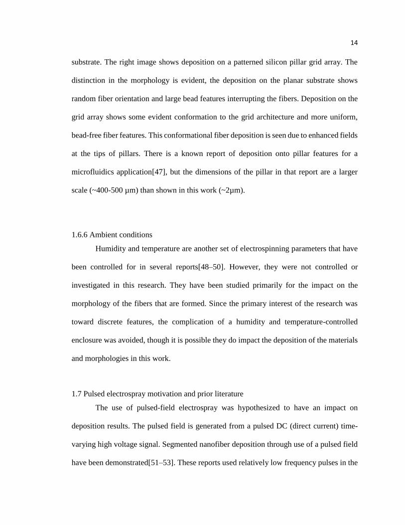
substrate. The right image shows deposition on a patterned silicon pillar grid array. The
distinction in the morphology is evident, the deposition on the planar substrate shows
random fiber orientation and large bead features interrupting the fibers. Deposition on the
grid array shows some evident conformation to the grid architecture and more uniform,
bead-free fiber features. This conformational fiber deposition is seen due to enhanced fields
at the tips of pillars. There is a known report of deposition onto pillar features for a
microfluidics application[47], but the dimensions of the pillar in that report are a larger
scale (~400-500 µm) than shown in this work (~2µm).
1.6.6 Ambient conditions
Humidity and temperature are another set of electrospinning parameters that have
been controlled for in several reports[48–50]. However, they were not controlled or
investigated in this research. They have been studied primarily for the impact on the
morphology of the fibers that are formed. Since the primary interest of the research was
toward discrete features, the complication of a humidity and temperature-controlled
enclosure was avoided, though it is possible they do impact the deposition of the materials
and morphologies in this work.
1.7 Pulsed electrospray motivation and prior literature
The use of pulsed-field electrospray was hypothesized to have an impact on
deposition results. The pulsed field is generated from a pulsed DC (direct current) time-
varying high voltage signal. Segmented nanofiber deposition through use of a pulsed field
have been demonstrated[51–53]. These reports used relatively low frequency pulses in the

15
single to ten hertz range. To our knowledge, pulsed-based electrospinning has not been
reported in the range of frequencies greater than this. A goal in this research was to
demonstrate tunable control over the deposition process via frequency and waveform
parameters in the applied voltage used to generate the field for electrospinning.
To validate this approach to electrospinning, a lab-built high voltage amplifier was
assembled using transformers to generate a periodic signal in the kilovolt magnitude range.
This setup allowed for testing proof-of-concept that higher frequency (tens to hundreds of
hertz) pulsed electrospinning is feasible, and the repeatability of using this setup.
Depositions with frequencies as high as 500Hz were reliably achieved. A picture showing
the internal electrical components is shown in the left panel of Fig 1.6. The right panel of
the same figure shows an oscilloscope screenshot demonstrating the output signal given an
input signal. The yellow color waveform is the input low voltage signal (here ~1Vpp) and
the blue waveform is the high voltage output signal (~3.5kVpp). Clearly there is a lack of
fidelity between the input and output signals, due to the transformer components used in
the system.
Figure 1.6: Early high voltage pulse system used (Left) Picture of main electrical components
of system (Right) Oscilloscope waveform showing input waveform (yellow) and output
waveform (blue).

16
Later in this project a Trek 10/10 high voltage amplifier was purchased by the
project sponsor. This system provides 1,000:1 amplification of a low-voltage input signal
with incomparably better fidelity than the lab-built transformer-based system and is
operable at a much wider range of frequencies.

17
Chapter 2: Pulsed-field electrospray and characterization of discrete nanoparticles
2.1 Introduction
A motivation in this work was to develop methodology for electrospray deposition
of discrete, oriented features. It was hypothesized that gas phase orientation of molecules
could be selectively controlled through frequency and/or waveform parameters of a high
voltage pulsed signal. This differs in approach to most electrospinning which uses a
constant DC voltage to generate nanofibers. Initially, to conduct experiments in pulsed
electrospray, we developed a transformer-based high voltage pulse system. This system
was used successfully for pulsed depositions but had limitations and was eventually
replaced with a commercial high voltage amplifier.
The material that saw the most use in this work for electrospray of discrete features
was the protein fibrinogen. Fibrinogen is a large (~340 kDa) protein with a rod-like
structure[54]. For this reason, it was selected early on as a material of interest to use in
conducting experiments on pulsed deposition and orientability. Electrospinning of
fibrinogen nanofibers has been reported by Wnek, et al. using a method to prepare a
solution of fibrinogen in 1,1,1,3,3,3-hexafluoro-2-propanol (HFP)[12]. The process they
reported used a stock preparation of the protein at a concentration of 83 mg/mL in minimal-
essential-medium (MEM), prior to 9:1 dilution into HFP. Reports have been published on
using electrospinning to produce biological-based nanofibers from fibrinogen[12] or
collagen[11] and achieving results that mimic the extracellular matrix[55,56]. Research has
also been conducted on the use of fibrinogen to fabricate biological-based bandages in
applications for assisting wound healing[57].

18
Attempting to prepare fibrinogen for electrospinning, we found that using a solution
preparation without MEM allowed for creation of non-fibrous, nanoscale-dimensional
fibrinogen structures. These discrete feature morphologies lent themselves to being more
applicable toward the study of electrical parameter effects on potential orientation during
the deposition process.
2.2 Materials and methods
2.2.1 Materials
Fibrinogen (from bovine plasma) was purchased from Sigma (St. Louis, MO,
USA). Bovine serum albumin from VWR (Radnor, PA, USA). Ammonium acetate from
Mallinckrodt AR (Staines-Upon-Thames, Surrey, UK). Sodium chloride from EMD
(Burlington, MA, USA). Polycaprolactone (Capa 6800) was obtained from Perstorp
(Malmo, Sweden). Polyvinyl alcohol (99% hydrolyzed, MW 89kDA-98kDa) from Sigma-
Aldrich (St. Louis, MO, USA). Purified DI water was obtained using a Milli-Q water
purification system from Millipore (Burlington, MA, USA). Hexafluoro-2-propanol and
trifluoroethanol were purchased from TCI America (Portland, OR, USA). Trifluoroethanol
was also purchased from Sigma (St. Louis, MO, USA). Chloroform came from J.T. Baker
(Phillipsburg, NJ, USA). Conductive adhesive copper tape was from 3M (St. Paul, MN,
USA). Syringes used were from BD (Franklin Lakes, NJ, USA). Syringe needles were
industrial dispensing tips from CML Supply (Lexington, KY, USA).

19
2.2.2 Development of lab-built transformer-based high voltage pulse system
2.2.2.1 System development and function
The lab-built setup was a cost-effective way to begin research into pulsed
electrospinning (new high voltage function generators or amplifiers are an expensive piece
of lab equipment). Mark Warner, formerly of the Oregon State Chemistry Department
Electronics Shop, assisted in development, design and testing the transformer-based system
in its first iterations.
The system functioned by using a low voltage input signal to generate a high
voltage output in the kilovolt range (up to ~8kV). The primary component in the high
voltage generation was a high voltage transformer. The high voltage signal, output from
the transformer, was rectified using a high voltage diode to retain only the DC component
of the signal. A 50MOhm resistor was added in series between the rectifying diode and the
high voltage output of the system to act as a current limiter and keep output currents in the
low 100µA ranges. The low-voltage signal was input to the system from a function
generator (Tektronix CFG250). The signal was amplified using an audio frequency-range
subwoofer amplifier and further stepped up by an audio frequency-range transformer
(Hammond 1640SEA) to voltages in the 100VAC range. This is an appropriate magnitude
of input voltage for the high voltage transformer, which was rated for operating with mains
voltage on the primary coil.
Audio frequency range components were chosen for the circuit elements, where
possible, to give the best fidelity frequency response over a range of frequencies. Though,
that range was most notably limited by the high voltage transformer, which is generally not
intended for use at frequencies other than standard 60Hz from mains. Although, it was

20
found that the transformer used for the system has a resonant frequency in the 500Hz range
and a usable frequency range up to 1kHz. Usable frequency range being the range of
frequencies where high-voltage output magnitudes sufficient for electrospinning were
achievable. Usable frequency range does not mean that the waveform shapes generated
across the range of frequencies were comparable between any given frequencies in that
range. In fact, the greatest limitation of this system was the inability to control aspects of
the pulse shape across a range of frequencies. The wave shape, peak-to-peak amplitude,
and DC offset of the generated high voltage signal were all functions of the input frequency,
waveform and amplitude. Therefore, it was usually not possible to maintain the same high
voltage signal parameters at different frequencies and make exact comparisons. Because
of this, the system did not allow for rigorous testing of electrospray behavior with directly
comparable parameter sets at different frequencies, yet it did provide a means to investigate
the feasibility of pulse-based electrospinning and demonstrate that it is readily practicable.
2.2.2.2 System iterations
Throughout its use the transformer system saw several design iterations and
replacements of components. There were three different audio amplifiers used in different
iterations of the system for the first-stage, low-voltage amplifying step. All were purchased
as a developed amplifier board, not as individual amplifier integrated circuit components.
Initially, a 68W LM3886 Class AB amplifier board by Yuan-Jing was used. This amplifier
had thermal issues in use in the high voltage system and several were destroyed before it
was decided to switch to a low-power/low-heat digital amplifier. A Sure Electronics AA-

21
AB31316 1x400W Class D Audio Amplifier was then used. Later, another Class D
amplifier, the TDA 7492 amplifier board (purchased from Parts-Express), was used which
was compatible with a smaller, lower-voltage power supply and the amplifier itself
required less space. This would have allowed for developing the high voltage system into
a more compact footprint, but this wasn’t done before the transformer system’s use was
discontinued in favor of the Trek amplifier.
The first high voltage transformer used in this system was a Webster/Xerox Type
44324 transformer designed for use as an ignition in oil burning boilers. It was rated for a
7kV secondary voltage with a 115V primary voltage. It also had the secondary end-point
grounded, with no center-tap, so only one connection to the secondary coil was accessible.
This was later replaced with a “Steinville”/”Well” transformer designed for 5kV peak-to-
peak voltage output. The schematic for this final iteration of the system is listed in Figure
A.1 in Appendix A.2. Frequency range output responses were also characterized for
maintaining specific output parameters and the details of this are listed in Appendix A.1.
The Well transformer showed better peak-to-peak voltage magnitudes in the commonly
used 100-500Hz frequency range than the Webster/Xerox transformer. However, the Well
transformer was not potted in an insulator (like the Webster transformer) so there were
issues reaching the same output voltages (greater than 5kV) as the Webster transformer.
Static/arcing/breakdown noises were heard when trying to operate the system above 5kV.
Testing the system in a low-light environment showed that arcing was occurring around
uninsulated portions of the transformer. The Webster transformer was a more stable option

22
for higher voltage use. If the transformer-based high voltage system saw continued use,
that would serve as a better component choice.
2.2.3 Solution preparation method development
One of the first materials electrospun on this project was the protein keratin in a
mixture with polyethylene oxide (PEO) in trifluoroethanol (TFE), based on a preparation
method reported in literature[38]. That solution was prepared with a 20 mg/mL
concentration of keratin/PEO in TFE and rapidly coated (over several seconds) substrates
during electrospray experiments (SEM image of results shown in Figure 1.2 in Chapter 1,
section 1.5.1). Also, the morphology of this material was deposited as nanofibers. It did
not respond to a pulsed DC waveform and segment into fibers. We sought to deposit
material less rapidly and as discrete features so instead prepared fibrinogen electrospinning
solutions at concentrations of protein at 5 mg/mL which is a significantly lower
concentration than reported by Wnek et al. Initially, attempts were made to dissolve
fibrinogen in TFE but it was not soluble in the solvent alone, so use of surfactants were
studied to assist dissolving the protein. Solutions with 5mg/mL fibrinogen were prepared
with 1 mg/mL surfactant in TFE. Surfactants used were cetyl trimethylammonium bromide
(CTAB), capstone, and sodium dodecyl sulfate (SDS). The solutions were left to mix
overnight on a rotisserie, but still appeared undissolved the next day. Solutions of 1 mg/mL
protein were prepared with concentrations of 5, 25 and 50 mg/mL surfactant in TFE. But,
none of the prepared solutions resulted in successfully dissolving the protein, though
increased surfactant concentration appeared to decrease the size of the undissolved

23
particles. Fibrinogen could be dissolved at concentrations of 1, 5 and 10 mg/mL in either
9mg/mL NaCl (saline) or 100mM Tris-HCl pH 7.0. Attempts to electrospray 5 mg/mL
fibrinogen from 100mM Tris-HCl were not successful and no spray behavior was seen.
Ammonium acetate of 4.8 pH and 100mM was used to attempt to dissolve 1, 2.5, 5 and 10
mg/mL fibrinogen. Only the 1 mg/mL fibrinogen was successfully dissolved.
Fibrinogen solution preparation in TFE was attempted with additions of MEM. A
ratio of 2 parts MEM to 8 parts TFE and 1mg/mL fibrinogen did not dissolve. Following
Wnek et al and attempting to use HFP as the solvent system with 9:1 HFP to MEM with
both 1 and 5 mg/mL fibrinogen was also not successful. Preparation of 1 mg/mL fibrinogen
with 20 mg/mL SDS in HFP resulted in a clear, dissolved solution. Electrospraying this
solution gave bead-like and granular morphology, likely influenced by the high surfactant
to protein ratio.
Preparation of fibrinogen for electrospinning involved a several step solution
preparation process. For the most successful preparation method, determined
experimentally, the protein is first dissolved into a stock solution before preparation in
HFP. The stock solution preparation method that proved the most successful was based
from the manufacturer product page[58] and used saline (9mg/mL NaCl) and gentle
agitation. Stock concentrations of the protein ranging from 10 mg/mL up to 200 mg/mL
could be prepared in a saline solution. There was hesitancy to using saline-based solution
preparation, due to incorporating addition non-volatile components to the solutions. As an
alternative, ammonium acetate was substituted and stock solutions were prepared with this
volatile salt instead. The stock preparation could then be diluted into the HFP solvent

24
system. Final dilutions of 5 mg/mL and 10 mg/mL were most frequently used. At higher
concentrations there was significant crashing out from solution of dissolved material and
resulting electrospray deposition morphology was large agglomerated particles.
Preparation of fibrinogen stock solutions without salt additives was also possible, but
higher concentration stock solutions was facilitated by using NaCl or ammonium acetate.
This solution preparation method was developed using fibrinogen but proved to be
applicable for preparation of bovine serum albumin (BSA) solutions in HFP. In these cases,
BSA was prepared in a phosphate buffered saline solution of pH 7.4 and diluted to final
concentration of 5mg/mL in HFP. Deposition of this solution showed quite comparable
morphologies to fibrinogen deposition. It is shown in Chapter 3, section 3.5.1.
2.2.4 Parameters used for electrospray deposition
Initially the solution preparation of 2 mg/mL fibrinogen (from 10 mg/mL stock in
DI H2O) was the primary approach used for electrospray. However, the preparation to
either 5 mg/mL and 10 mg/mL (from 200 mg/mL stock in 9 mg/mL ammonium acetate)
was used the most extensively, due to it being a more reliable solution to work with, having
a more rapid rate of deposition during electrospray, and generating more discrete deposited
morphologies.

25
Electrospinning of fibrinogen nanoplates was most successful at 1.5kV-2kV per cm
needle-to-collector distances with the optimized deposition distance being 3cm with 5.5kV
applied potential. Unless otherwise noted, fibrinogen samples were prepared by
electrospray of the solution dispensed from a 3mL BD luer-lock tip syringe, fitted with a
22-gauge blunt-tipped syringe needle, onto a 1cm x 1cm square coupon of silicon wafer at
a flow-rate of 50µL/hr. The silicon coupons were mounted and electrically grounded to a
metal post using double-sided copper tape with a conductive adhesive. A good example of
the deposition pattern on these substrates is shown in Figure 2.1 with a circular pattern.
Deposition density was typically gradient from the center to the outer edge of the spray
area. It did not always center on the substrate and in some cases would overlap the edge of
the silicon.
2.2.5 Silicon substrate cleaning procedures
Non-patterned silicon substrates (shown after use for electrospray in Figure 2.1)
were cleaned prior to use. The method used sonication in solvents: acetone, methanol,
Figure 2.1: Electrospray deposition onto 1cmx1cm silicon
wafer coupons. Here mounted on pin stub holders prior to
SEM imaging.

26
and DI H2O. This step was done after silicon wafers had been diced into 1cm x 1cm
coupons. Both variations on the cleaning procedure listed below were useful to remove
some of the debris from the substrates that was left after wafer dicing.
10-minute per-step single sonication with rinse:
1. 10-minute sonication in acetone
a. Rinse substrates individually with acetone
2. 10-minute sonication in methanol
a. Rinse substrates individually with methanol
3. 10-minute sonication in DI H2O
a. Rinse substrates individually in DI H2O
4. Dry substrates individually using dry nitrogen gas
5-minute repeat sonication:
1. 5-minute sonication in acetone
a. Replace acetone and repeat sonication
2. 5-minute sonication methanol
a. Replace methanol and repeat
3. 5-minte sonication in DI H2O
a. Replace DI H2O and repeat
4. Dry substrates using dry nitrogen gas
2.2.6 Image based feature characterization
2.2.6.1 Image collection
Scanning electron microscopy was used for collecting images of electrospun
samples. The scanning electron microscope used was a FEI Quanta 600 in the Oregon State
University Electron Microscopy Lab. Samples usually were prepared with sputter-coating
prior to imaging to address charging and poor contrast issues as most of the deposited
materials worked with were non-conductive. Sputter-coating with Au/Pd was generally
done for 35 seconds. Most images were collected with a 5kV accelerating voltage. The

27
relatively low voltage was used due to the electrospray deposited materials generally
having sensitivity to higher accelerating voltages.
2.2.6.2 Image segmentation and feature characterization
Image segmentation is a nebulous process which is facilitated by obtaining proper
images as much as the proper application of processing techniques. Images need to be taken
with consideration toward the later application of segmentation. Many images obtained
throughout the collection of data for this work do not have high contrast. Without this, the
images’ histograms do not have distinct peaks. The images cannot be segmented by a
simple pixel intensity threshold approach alone. More complex segmentation algorithms
must be applied, which still require tuning to generate the desired results; this is the nature
of image segmentation. Only qualitative observations can be made without successful
application of segmentation to extract quantitative measurements from images. Still, there
is variability in the results obtained from different approaches to segment and extract
quantitative measurements from the images.
The Feret diameter was considered the most relevant measurement of the
electrosprayed features, since it is measured as the longest distance across a particle feature
and provides a means to measure the distribution of electrosprayed particle sizes. Several
segmentation algorithm approaches were applied to determine their variability to the
resulting size measurements. ImageJ and FIJI software were used for image processing to
measure the Feret diameter of deposited nanoparticles using the Particle Analysis tool in
the BoneJ plugin extension to FIJI. The processing steps of filtering, segmentation, binary

28
operations (erode, dilate, hole fill, watershed) and particle size analysis were all performed
within ImageJ. The generated arrays of Feret diameter measurements were exported to
MATLAB for computing a distribution plot of size-binned feature measurements (particle
size histogram). MATLAB was also used for plotting graphs of the data. A more
comprehensive script could be implemented, entirely using MATLAB for image
processing, segmentation, extraction of measurement data and graphing of this data. But,
that was not achieved for this work.
The image in Fig. 2.2 is electrospray deposited polyvinyl alcohol (PVA) used in
developing image segmentation approaches for making quantitative measurements from
SEM image data collected during this research. The image shows some distinct contrast
between the background and the deposited features. However, there are not separate peaks
in the histogram, so a simple intensity threshold is not applicable. A median filter of 2.0-
pixel size was used to address background noise in the image. Three segmentation
Figure 2.2: Electrospun polyvinyl alcohol (PVA)
particles.

29
algorithms were applied to compare results: unsupervised K-means, supervised Hidden
Markov Model, and supervised K-means. These segmentation approaches operate on pixel
intensity and separate the image into regions by labelling as one of a pre-defined number
of classes. Three color classes were used with each segmentation approach. Each resulting
array of feature size measurements were sorted into size distribution bins of 50 nm width
(~5 pixels for SEM images recorded at 11µm horizontal field width (HFW) and ~10 pixels
for an HFW of 5 µm). Features with a Feret diameter ~20nm were removed, due to these
likely being noise features from segmentation and features of this size were not visually
recorded in hand measurements, so they are not expected to represent deposited features.
The size histogram counts were normalized to the total number of counts to allow direct
comparison between size histograms from different samples with differing numbers of total
feature counts. Between the filtered, size-binned Feret measurements from different
segmentation approaches the mean and error of the percent of binned counts was computed.
The results of the three segmentation methods applied to the image in Fig. 2.2 is shown by
the graph in Fig. 2.3. There is variation in the size measurement distribution based on the
segmentation approach used, introducing possible error. Ultimately, the choice was made
to use the automatic k-means segmentation approach. The supervised k-means cluster and
hidden markov model both required training the algorithm on each image to be segmented.
To process multiple images from multiple samples, this was not feasible from a user
perspective. Both user time and, by involving a user, the possibility to introduce
inconsistencies in class selection. The automatic approach allowed the incorporation of the

30
tool into an ImageJ macro process to crop, filter, segment, apply binary operations, and
measure particle features.
2.3 Results and discussion
2.3.1 Electrospray deposition of discrete nanomaterials
Throughout this research has resulted in the ability to deposit discrete feature
morphologies from various materials of protein or polymer. Examples of these are shown
in Fig. 2.4. These features have all been deposited using low concentrations of material in
solution (5 – 10 mg/mL) which is conductive to depositing these morphologies. In cases
where the morphology and size of the deposited features was studied, the collection
substrate used was a 1cm x 1cm coupon of silicon wafer mounted on an aluminum foil
backing (3cm x 3cm). The silicon coupon was attached to the foil with a double-sided
Figure 2.3: Mean size distribution of electrospun polyvinyl alcohol (PVA)
particles with error shown between comparison of different segmentation
approaches.

31
conductive adhesive copper tape and the foil was mounted on a grounded metal post using
the same tape.
Electrospray was demonstrated with DC deposition when a sufficient field strength
was reached. Operating field strength was dependent on the solvent system used. Volatile
organic solvent systems required strengths in the range of only 1.5-2 kV/cm (hexafluoro-
2-propanol, trifluoroethanol). Whereas when working with aqueous systems 2 kV/cm was
typically the lowest possible field strength where electrospray occurred. The DC voltage
where the onset of stable electrospray of fibrinogen began was recorded at several working
distances listed in Table 2.1.
Figure 2.4: Electrospun proteins (fibrinogen, bovine serum albumin) and
polymer (polyvinyl alcohol).

32
Electrospray of
fibrinogen
2cm 3cm 4cm
Onset Voltage 4 kV 4.5-5 kV 6 kV
Field Strength 2 kV/cm 1.5-1.67 kV/cm 1.5 kV/cm
The required field strength was observed to decrease with increased deposition distance in
electrospray of this solution. A wider range of distances was possible for electrospray.
Deposition at a distance shorter than 2cm was usually not practical because unevaporated
solvent could be collected. Deposition could also be achieved at distances greater than 4cm
(by adjusting voltage appropriately) but at longer distances the spray area was typically
larger than the substrate. This 2cm-to-4cm needle-to-collector distance range was the space
predominantly used.
Parameters could be noted for electrospray deposition with a pulsed DC, time-
varying signal in several ways. The transformer system initially used had a frequency
dependent peak-to-peak voltage. While this behavior was characterized, the RMS voltage
of the signal was used to make comparisons between electrospray at different frequencies.
Depositions were achieved at frequencies ranging from 60Hz to 500Hz. Though, in the
upper range of frequencies, the peak-to-peak voltage was diminished, compared to lower
frequencies. Fibrinogen was first stably deposited using a 5.3kVrms, 120Hz signal at a 3cm
deposition distance. This agrees with (several hundred volts above) the minimum onset DC
voltage for this distance, which was determined later (listed in Table 2.1).
Table 2.1: DC electrospray onset voltage for deposition of 10mg/mL fibrinogen in HFP.

33
After transitioning to use the Trek 10/10 high voltage system, noting and
controlling more parameters of the signal was appropriate because these aspects of the
signal parameters were fully adjustable with the Trek amplifier. Peak-to-peak voltage and
DC component offset are a reproducible description which can be set at different
frequencies.
2.3.2 Electrosprayed morphologies and relation to solution parameters
The earliest successful technique used in this research to deposit protein
nanoparticles was by preparing fibrinogen at a concentration of 10 mg/mL in DI H20 and
allowing to dissolve at room temperature over a period of several days. The stock solution
was then diluted 1:4 in HFP for a final concentration of 2 mg/mL of fibrinogen. This
solution could be readily electrosprayed and is shown in Fig. 2.5 after deposition on a
coupon of silicon wafer. Electrospray deposition of this fibrinogen solution showed a
distinctly flake-like morphology and was centered in localized regions which showed a
Figure 2.5: Electrospun 2 mg/mL fibrinogen on Si coupons. (Left) Top down view. Scale
at 10um (Right) Cross-sectional view of cleaved wafer sample. Scale at 5um.

34
structure oriented upward from the substrate surface. The depositions shown in the figure
were performed using the transformer based high voltage system (detailed in section 2.2.2)
at a 120Hz pulsing waveform with an effective 5.3kV DC component at a needle-to-
collector distance of 3cm with a dispensing flow rate of 50 µl/hr.
Electrospraying fibrinogen solutions with 2 mg/mL dilutions in HFP, from varied
stock solution concentrations, showed varied morphology results. The results are shown in
Fig. 2.6 of the resulting morphologies from electrospray of solutions with 50 mg/mL, 90
mg/mL and 200 mg/mL wt. stock solutions diluted to 2 mg/mL final concentration of
fibrinogen in HFP. The benefit of the higher concentration stock is a reduced ratio of NaCl
to protein in solution, since all concentrations of protein were prepared using the same
concentration of NaCl (saline, 9mg/mL). However, none of these results showed distinctly
discrete morphologies. Preparation of the dilute solution at 10 mg/mL in HFP from 200
mg/mL stock in saline gave a distinctly different resulting morphology shown in Fig. 2.7,
Figure 2.6: Electrospun 2 mg/mL fibrinogen on Si substrates. Dilutions prepared
from stock concentration into HFP solvent system. (Left) From 50 mg/mL stock
(Middle) From 90 mg/mL stock. (Right) From 200 mg/mL stock. Scale bars are at
1um.

35
also deposited using the transformer pulse system. These results show a “cupped” shape.
There is a definite distribution in particle size, but features tend to the sub-micron range
and most heavily in the 100-300nm range.
2.3.3 Voltage parameters effect on electrospray of fibrinogen
Electrospray of fibrinogen nanoparticles showed variation in deposition comparing
pulsed DC to DC deposition. The parameters compared were DC at a 6kV magnitude
voltage and pulsed 50% duty cycle square wave with 3kV peak-to-peak voltage (minimum
at 3kV, maximum 6kV). These pulsed depositions were done using the Trek high voltage
amplifier. By choosing a minimum voltage at half of the maximum, there should be no
electrospray occurring during that portion of the period of the pulsed waveform. Difference
in deposition density is apparent between DC and pulsed DC in the SEM images shown in
Fig 2.8. All samples were prepared using a 30 second deposition, so this density difference
between DC and pulsed parameters can be accounted for by the periodicity of the pulsed
DC waveform, which has less time over the deposition where there is sufficient field to
cause electrospray.
Figure 2.7: Electrospun 10 mg/mL fibrinogen
from 200 mg/mL stock. Scale bar at 1um.

36
Image processing and segmentation in ImageJ was used to make quantitative
feature size measurements and comparisons between the images. The process used was:
median filter (2.0-pixel size), background subtraction, segmentation (automatic 3-color-
class k-means cluster), threshold to binary, binary operations (erode, dilate X2, hole fill,
erode, watershed), and finally BoneJ particle analysis to collect Feret diameter
measurements. To compare the pulsed DC and DC parameters results, five samples of each
parameter set (DC, 100Hz pulse, 500Hz pulse) were prepared. The images in Figure 2.8
are an example from each parameter set. From each sample three images were collected
and processed with the image segmentation. The array of measurements from each of the
three images of a sample were combined and counted into sized bins of 50nm width (the
first bin is 0-50nm, though 20nm and below sizes are not considered). The counts in each
bin was normalized by the total number of measurements made across the three images.
There is quite significant variability in the distribution of small features (50-100nm)
between the DC deposition samples. The depositions with pulsed DC are consistent across
the size bins. In the 100-250nm size range the DC depositions show greater fraction of
distribution than the pulsed DC parameters.
Figure 2.8: Electrospun 5mg/mL fibrinogen on Si coupons. Scale bars 2um (Left) ES at DC
(Middle) ES at 100Hz (Right) ES at 500Hz

37
Based solely on visual inspection of the images, there are evidently more of the
largest feature sizes present on the pulsed DC deposited samples. This doesn’t show in the
distribution plotted in Figure 2.9, due to the graph scale being skewed toward high fraction
of distributions at the lower feature sizes. Viewing the numerical data which is plotted in
the graph reveals that the upper size features (500-100nm) are seen more in the pulsed DC
depositions than the DC, though these feature sizes are still a small minority compared with
the amount of small feature sizes. This numerical data is included in Table B.1 in Appendix
B, section B.2.
Figure 2.9: Size distribution of electrospun fibrinogen at DC, 100Hz and 500Hz
parameters. Size bins are 50nm in width.

38
Chapter 3: Electrospray deposition of protein nanoparticles for enhancing performance
of a microfluidic blood plasma separation device
3.1 Introduction
We have demonstrated the ability to electrospray protein as discrete nanoparticles.
There are multiple proteins and enzymes involved in the blood coagulation cascade which
could be considered for electrospray to increase blood coagulation on a separation
device[59]. The ability to electrospray fibrinogen, a protein involved in blood coagulation,
motivated the application of electrospray deposition for enhancement of the performance
of a microfluidic blood plasma separation membrane device. Electrospinning has been
reported in literature[60–63] for blood separation applications by fabrication of electrospun
filtration membranes but, to our knowledge, no publications exist on electrospray
deposition of blood coagulation chemistries for blood plasma separation applications.
3.2 Motivation for application to a blood plasma separation device
Fibrinogen is a protein which is involved in the blood coagulation cascade. During
blood clotting fibrinogen is cleaved into fibrin by the enzyme thrombin and polymerizes
as fibrin[54,64]. Fibrin forms as fibers, which act to bind up red blood cells in the blood
and form clots[54]. We were motivated to electrospray fibrinogen nanoparticles toward an
application with a microfluidic blood plasma separation device developed from glass
microfiber membrane in Remcho Research Group as part of a student’s thesis work[65].
The goal was to enhance coagulation by introducing additional coagulation chemistries.
The microfluidic membrane device does not rely on instrumentation and is applicable to
quantitative point-of-care analysis; which facilitates its employability in resource limited

39
areas without access to clinical laboratories or as an easy-to-use, single-use analytical
device for in-lab applications[65]. It relies on hydrophilic surface chemistry to cause
wicking fluid flow on the membrane and is single-use for this reason – after use with fluid,
it will no longer wick fluid. Electrospray is a compelling technique for modifying the
device after fabrication, since the membrane is not exposed to any solvent during the
deposition process which avoids altering its hydrophilic surface chemistries.
3.3 Function of blood plasma separation membrane device
The membrane device is capable of separating blood samples into two fluid
components: the red blood cell and plasma (or serum) components[65]. Whether serum or
plasma is the separated component in the device depends on whether the blood has been
treated with an anticoagulant. Serum is fluid remaining after blood clotting and is a
component of plasma but contains no coagulation chemistries (they have been involved in
the blood clotting)[66]. Plasma separates from blood which has been treated with an
anticoagulant, so the coagulation chemistries remain in the liquid[66]. Fresh blood samples
will coagulate on the device, so the fluid which separates from the red blood cell containing
fluid will be serum. Anticoagulant treated blood samples will be separated as red blood cell
fluid and plasma fluid components.
Separation of these fluid components is achieved through lateral flow of the fluid
sample on the membrane device. Initially, glass microfiber is hydrophilic, but in the device
fabrication, the membrane is filled with the polymer polycaprolactone (PCL) and rendered
hydrophobic[65]. Fluid flow channel features are patterned into the device via selective

40
oxygen radical exposure (ORE) through a mask which defines the desired features. This
ORE step renders the exposed areas hydrophilic via surface energy activation. The result
is a hydrophilic channel feature patterned into a hydrophobic membrane device. Fluid
introduced into a circular sample zone at one end of the channel is wicked by the
hydrophilic surface to flow down the channel. When a blood sample is introduced to the
membrane the subsequent flow along the channel results in a retention of the red blood cell
fluid component within the matrix more than the plasma (or serum) component. This allows
for assay to be performed on the less retained plasma (or serum) component[65].
Blood tests were performed on two styles of separation membrane. The first device
(shown in Fig. 3.1) has a patterned loop structure, with surface flow on both top and bottom
of the membrane. After a blood sample is introduced on the top surface, it first flows
through a via to the bottom surface, then flows along a channel on the bottom surface before
finally returning to the top surface through another via and flowing along a channel to an
assay region. Electrospray deposition was done onto the bottom surface flow channel. The
second style of device (Fig. 3.2) does not use any via structure and has separative flow in
a surface channel on one side of the device.
Figure 3.1: Loop structure blood separation device (Left) Serum (clear fluid circle)
can be seen reaching the top of the via, returning to the top surface (Right) At a later
point in time, red colored fluid (containing red blood cells) is now reaching the top of
the via.

41
3.4 Methods
3.4.1 Electrospray onto membranes
Conducting these experiments required devising a setup for electrospraying onto
the membrane devices. Typical electrospray collectors are conductive (metal foil) or semi-
conductive (silicon) materials. By mounting the membrane onto a grounded conductive
backing we were able to generate electrospray that collected on the membrane. Masking
off specific regions of the channel on the membrane device allowed for functionalizing
selected regions with the fibrinogen nanoparticles. Shown in Fig. 3.3 is comparison of the
membrane device with and without nanoparticle functionalization, demonstrating how
these features appear (on the micro-scale) when deposited onto the device using the
Figure 3.2: Separative blood flow on a single-sided membrane device depicted at several
points during the process. 1) Sample is introduced 2) Some separation of the fluid
components is visible 3) The separated plasma component of the sample has reached the
end of the functionalized region 4) Red blood cell fluid component has reached the same
point 5) After flow is complete

42
electrospray technique. No macro-scale images of devices after functionalization with
electrospray are included, because the glass microfiber membranes are white and
electrosprayed fibrinogen also has a white appearance.
3.4.2 Measurement of device performance
Flow performance across the masked surface deposition region was compared
between functionalized and non-functionalized channels (control). The rate of fluid flow
was measured as the difference in time between the two separated fluid fronts reaching the
same point on the channel, at the end of the functionalized region. The clear plasma (or
serum) component flows faster, so the time between this component reaching the end of
the surface deposition region and the red blood cell component reaching the same point is
measured as the separation time and indicates the efficiency or strength of the separation.
Comparing the separation time between channels functionalized with the nanoplates versus
un-functionalized (control) channels shows how the electrospray functionalization affects
the flow behavior. A drawing of the later surface flow separation is shown in Figure 3.4,
indicating the separative flow over the functionalized region. To minimize variation in
Figure 3.3: (Left) Un-modified, control membrane (Right) Membrane modified with
electrospray deposited nanoparticles

43
results due to the variability in the device fabrication, control channel flow was measured
on each device. The separation time on control channels was used to normalize the flow
time on functionalized channels on each device. Then, normalized separation time was
comparable between devices.
3.5 Results and discussion
3.5.1 Protein materials deposited
Another comparison method used in these experiments was the deposition of a
protein not used in blood coagulation, bovine serum albumin (BSA), to determine how
fluid flow is effected by a material with similar morphology to the fibrinogen nanoplates.
Shown in Fig. 3.5 is comparison of electron microscope images of deposition of BSA and
fibrinogen nanoparticles on the membranes.
Figure 3.4: (Left) Diagram of blood separation behavior on lateral surface flow channel.

44
3.5.2 Test with control fluid
If fibrinogen specifically interacts with a fresh blood sample, and causes an increase
in coagulation, then increased separation time (between the plasma and red blood cell
component) would be seen with only the fibrinogen functionalized channels and not those
functionalized with BSA. To see how fluid flow is generally impacted, phosphate buffered
saline (PBS) of pH 7.4 with a color dye was used to compare the affect on the flow times
of a non-blood fluid sample across control, fibrinogen functionalized, and BSA
functionalized channel regions. These flow time data are shown in Fig. 3.6 with flow times
on fibrinogen and BSA coated channels normalized to the control flow time. Though there
is variation in the mean flow time, there is not a significant impact due to the presence of
electrospray deposited protein nanoplates.
Figure 3.5: (Left) Fibrinogen nanoparticles deposited on the membrane device. (Right)
Deposited bovine serum albumin nanoparticles.

45
3.5.3 Device testing with blood samples
Blood samples used for the blood separation performance testing were collected
from canine sources. Fibrinogen deposited on the membrane devices was sourced from
bovine plasma. It should be noted that this cross-species aspect is not an issue, generally
any mammalian fibrinogen can interact with any mammalian thrombin in coagulation[58].
The impact of protein nanoplates on separation performance was compared with both
EDTA-treated and fresh blood samples. EDTA is a chelating agent for metal ions, such as
calcium, and is used as an anti-coagulant treatment for blood samples[67]. It functions by
binding to calcium[67] in the blood, which is a catalyst for the conversion of fibrinogen to
fibrin. This cuts off the route for fibrinogen’s involvement in blood coagulation. If
fibrinogen nanoplates deposited onto the separation device through electrospray can
interact with the blood sample and affect coagulation, there should be a more significant
impact on the flow of a fresh blood sample than on an EDTA treated sample.
Figure 3.6: Mean flow time of a non-blood fluid sample across protein nanoplate
functionalized and control regions of the separation membrane.

46
3.5.4 Blood separation results
What as observed, however, was a remarkably similar impact on the flow time of
both fresh blood and EDTA treated blood, when blood separation was done on a fibrinogen
functionalized membrane channel. These flow time results are shown in Figure 3.7, with
the flow times in the functionalized channels normalized by the flow time of the control
(non-functionalized) on the same device.
This similarity in flow behavior is indicative that the fibrinogen may not
specifically affect coagulation of the blood. Membrane channels functionalized with BSA
nanoparticles also show an increase in the flow time, though not as significantly as
compared to the fibrinogen functionalized. Shown in Fig. 3.8 is the compared flow times
Figure 3.7: Separation time between RBC and plasma fluid components testing
with EDTA and fresh blood samples on BSA and fibrinogen functionalized
channels, normalized by control.

47
of only the plasma component of an EDTA treated blood sample on fibrinogen versus BSA
functionalized channels.
This was measured as the time from introduction of the sample to the device to the
time when the plasma fluid flow reached a marked point on the channel. Again, these flow
times are normalized to the flow time of sample on the control (non-functionalized)
channel. In this case, the flow time on the fibrinogen coated channel is about twice that of
the control. The flow time of the plasma component on the BSA functionalized region does
not differ significantly from the control flow time.
Since fibrinogen deposition shows a similar effect on the separative flow of both
fresh and anticoagulant-treated blood samples, it is not conclusive that the protein is
impacting coagulation. While a similar effect from the fibrinogen is also seen on the flow
time of the plasma, the BSA does not notably impact the flow. So, it is also not conclusive
Figure 3.8: Flow time of plasma fluid component on BSA and fibrinogen
functionalized channels, normalized by control.

48
whether the protein nanoparticle features are simply impeding the flow of the blood
sample.

49
Chapter 4: Electrospray deposition of the glucose oxidase enzyme for an
electrochemical glucose sensor application
4.1 Introduction
A primary goal in this research in electrospinning/electrospray was to develop the
ability to manipulate and control the deposition of discrete nanomaterials. Specifically, the
goal was to achieve tunable control over the orientation of deposited features via frequency
and waveform parameters of the high voltage applied during the electrospray process.
Proteins such as antibodies and enzymes are of interest for application of this study,
because orientation is a critical factor in the efficiency of antibody-antigen or enzyme-
substrate binding. Both have an active site which must be oriented favorably to allow
interaction with an analyte[68], [69]. Comparing signal response between sensors prepared
using different functionalization approaches is a compelling method to study the effect of
electrospray parameters.
4.1.1 Electrospray for sensor functionalization
Electrospinning has been applied for the purposes of electrode functionalization or
fabrication. Non-enzymatic electrospun fiber sensors have been demonstrated for glucose
detection[23,70–72]. Other electrospun fiber sensors for gas contaminants such as carbon
monoxide and hydrogen sulfide[25,26,73] have been fabricated using electrospinning.
Moisture sensitive electrospun materials have been applied to humidity detection[8,22,74].
Few have reported on direct electrospinning or electrospray of glucose oxidase enzyme
incorporation into electropun material for development of glucose sensors[75–77].

50
The controlled deposition of the enzyme glucose oxidase (GOx) was studied for the
application of electrochemical glucose detection. Prior literature has reported on techniques
involving electrospinning/electrospray and GOx functionalization. However, most of these
reports use electrospinning to fabricate a nanofibrous membrane mat and subsequently
immobilize the enzyme to the fiber in liquid phase[78–81]. Ge et al. demonstrated retention
of enzyme activity after electrospray deposition but notably, Ren et al. demonstrated
deposition of GOx incorporated into solution with the polymer polyvinyl alcohol (PVA)
for an electrochemical glucose sensor application[76]. However, the deposited morphology
is continuous fibers interrupted by bead morphologies. This is less desirable for a goal of
affecting orientation, since features are not discrete in the fibrous morphology and
attachment by continuous fibers could interfere with orientability.
4.1.2 Replication of reported method: enzyme functionalized fibers
Incorporation of 1mg/mL GOx into 10 mg/mL PVA (99% hydrolyzed) in an
aqueous solution was attempted for surface functionalization of an electrochemical sensor.
The resulting morphologies shown in Fig. 4.1 are comparable to results shown in Fig. 2(c)
in Ren et al. The resulting morphology achieved in this work has notably smaller bead and
fiber dimensions. We did not follow the full procedure they used with glutaraldehyde (GA)
vapor exposure to crosslink the PVA and GOx. As a result, the sensor demonstrated a
decaying signal during the additions of glucose to the electrochemical sensor environment.
This is likely due to the solubility of the PVA fiber support matrix without the use of GA
vapor for crosslinking.

51
4.2 Methods
4.2.1 Development of electrospray parameters for glutaraldehyde and glucose oxidase
As a path to go forward, developing PVA/GOx fibers using GA vapor exposure
was considered, however it was dismissed since the continuous morphology was less
desirable for orientation studies and the technique of electrospinning PVA/GOx fibers and
using GA vapor exposure had already been demonstrated by Ren et al. The option of simply
incorporating GA and GOx in a solution was then considered for depositing discrete feature
morphologies and achieving a stable sensor.
An aqueous preparation of 50 mg/mL glutaraldehyde (GA) and 1 mg/mL glucose
oxidase (GOx) was prepared and demonstrated to be readily applicable as an electrospray
solution. Shown in Fig. 4.2 – the left image is the Taylor cone behavior during electrospray
of the solution (in this case a pulsed high voltage waveform is applied). Stable Taylor cone
behavior was observed, meaning there was little variation in the shape of the cone during
the electrospray deposition. Shown in the right image of Fig. 4.2 is deposition of the
Figure 4.1: Electrospun PVA with GOx on Si coupon
from aqueous solvent system.

52
GA/GOx particles. Electrochemical experiments were carried out using a platinum
working electrode prepared by electrospray deposition onto the electrode surface, however
this surface was not feasible for imaging. This was due to the platinum electrode being
mounted on a glass barrel several centimeters in length (making it physically difficult to
image in an electron microscope), additionally the electrode could not be sputter-coated
without compromising its functionality as an electrochemical sensor. An optical
microscope was used to verify that material was indeed deposited on the surface, but the
individual morphologies were not visible because the features were too small. Planar
silicon wafer chips were used as a substitute substrate to collect images of electrospray
deposition. Although, Taylor cone spray behavior is notably different when compared
between electrospray onto the two types of substrate, as shown in Fig. 4.3. In this case, the
same electrospray parameters were used, the only difference being the type of substrate
used as a collector. Thus, the resulting morphology imaged by SEM on the silicon wafer
Figure 4.2: (Left) Electrospray deposition of apparent glutaraldehyde/glucose
oxidase nanoparticles and stable Taylor cone is achieved. (Right) SEM image
showing particles collected during electrospray.

53
chip may not be comparable to the morphologies collected by electrospray on the platinum
electrode.
4.2.2 Electrospray methodology
Though the resulting morphologies were not directly observable on the electrode
surface, the sensor functionalized by electrospray can still be tested by use
electrochemically to verify the presence of active enzyme. With the overall goal being to
demonstrate differences in the resulting sensor response between pulsed and DC
electrospray depositions, a baseline DC performance was first established. To compare
pulsed high voltage waveform depositions to the constant DC deposition, the pulsed signal
was set to have a maximum voltage at the constant DC level and a minimum at half the
maximum. This was chosen so that no electrospray should occur during the pulse minimum
time of the high voltage waveform. During the time that the waveform is at its peak there
is the same field strength as the constant DC voltage.
A general working space for electrospray parameters was determined
experimentally by starting from parameters established previously for aqueous
electrospray solvent systems. We have been successful electrospraying a 10 mg/mL
Figure 4.3: Electrospray using 40Hz sine wave pulse with 4kVpp and 4kVdc at a 3 cm
distance from needle to substrate. (Left) Electrospray at a silicon wafer chip substrate.
(Right) 500µm diameter platinum electrode.

54
aqueous solution of polyvinyl alcohol with a 2kV/cm applied field strength, so this was
considered as the starting point for electrical parameters. Since enzyme is not storable at
room temperature, electrospray was carried out immediately after preparation of the
GA/GOx solution. After electrospray, electrodes were either immediately used for
electrochemical tests or stored at 4C to minimize any degradation which could impact the
sensor performance.
4.3 Results of electrochemical sensor performance
With stable starting parameters for electrospray of the GA/GOx solution, the impact
on the sensor response due to variations in these parameters was studied; specifically, the
comparison between using DC and pulsed DC for deposition. The most stable sensor
performance with a DC deposition was achieved using parameters of 9kVdc applied with
a 4cm needle-to-collector distance for 30 second depositions. For this data, the change of
current response of the sensor to standard additions of analyte is normalized to the electrode
surface area and molarity of target analyte (glucose). Sensors prepared with these DC
parameters gave responses of 0.2, 0.3 and 1 µA/cm2.mM (N = 3). The most stable set of
sensors functionalized by pulsed deposition used the parameters of a 40Hz sine wave with
4kVpp at a 4kVdc offset over a 3cm needle-to-collector distance for a 30 second
deposition. This resulted in normalized responses of 0.5, 1.2 and 3 µA/cm2.mM (N = 3).
These results are compared in the graph in Fig. 4.4. There is significant overlap in the range
of sensor response between the two electrospray parameters (pulsed vs. DC) and the range
of variation of the sensor responses is quite large. Though, it may also be valid to note that

55
direct comparison of pulsed DC vs DC depositions performed for the same period of time
may not be entirely compatible. The pulsed parameters used had a voltage minimum at half
that of the peak voltage. This means that the necessary voltage to sustain electrospray was
not constantly provided (only for half of the period). The pulsed electrospray deposition
should then result in less material being deposited over the same period of time as a
constant DC deposition, provided the electrode surface is not already completely saturated
during the deposition time.
It must be noted that the magnitude of the response from electrodes prepared using
electrospray is much lower than the conventional direct pipetting/drop-casting approach by
one-to-two orders of magnitude. In the optimized drop-casting, functionalizing the
electrode with a volume of 0.3µL of solution gave a sensitivity of 60 µA/cm2.mM. It was
not considered initially to optimize to comparable volumes to compare between the
optimization for electrospray and drop-cast; an electrospray time of 30 seconds was chosen.
At a 50 µL/hr flow rate the 30 second deposition means ~0.4 µL of solution could be
Figure 4.4: Comparison of sensor response between pulsed DC (40Hz
sine wave) and DC deposition.

56
electrosprayed. Use of the 30 second deposition was continued, to make comparisons
between the electrospray results comparable, but as a result the volume of solution is not
comparable to the drop-cast results. Regardless, the drop-cast approach generated much
greater signal, so more value was to be found in comparing results between electrospray
parameters than comparing them to drop-cast. Because it is also likely that not all
electrosprayed material is collected on the electrode surface, comparison of the same
volume for drop-cast and electrospray may not be relevant anyway. It is also questionable
whether considering time and flow rate alone is enough to determine how much volume of
solution has been electrosprayed. Without being able to quantify the amount of material on
the electrode, from either preparation method, it is difficult to make comparisons between
the two.
There were several parameter sets for both DC and pulsed deposition that did not
show stable sensor response. For DC: 8kV at 3cm gave a high magnitude response (5
µA/cm2.mM) but had significant signal decay and cannot be considered a reliable response.
With pulsed deposition: 40 Hz sine, square and triangle waveforms at 4kVdc and 5kVpp
at 4cm distance and 30, 15, and 5 seconds depositions either gave no response or had
significant signal decay. Additionally, the sensors which were not stable for use as an
electrochemical electrode showed high capacitance, meaning that material was deposited
onto the electrode surface but was evidently not active for glucose interaction.
Unfortunately, comparing successful DC and pulsed DC parameters was not
achieved using the same deposition distance. A functional sensor was not achieved from
DC deposition at 3cm using constant voltage at 8kV (the peak voltage used with pulsed

57
deposition at 3cm). Likewise, a functional sensor was not achieved from pulsed depositions
at the 4cm distance using a peak voltage at 9kV (the constant DC voltage used in
depositions at 4cm). So, a comparable parameter set was not achieved for the same
deposition distance to allow direct comparisons to be made in that parameter.
Going forward, it would be preferable to develop parameters for pulsed DC and DC
depositions which allow comparing deposition at the same distances. The range of pulsed
parameters is a large space and making informative conclusions about pulsed depositions
requires having as comparable as possible of parameters, so the impact of pulsed DC can
be isolated. These results, showing such variability in sensor stability from different
electrospray parameters, are evident of the stability having high dependence on the
parameters used. It is not clear how exactly the parameters impact the stability in these
cases. Active enzyme could be present on the electrode surface, but unable to conduct
current to the electrode – so no signal is detectable. Enzyme could have been deposited in
a way where its active sites were not accessible to the glucose. It is not possible to conclude
the exact impact on the enzyme deposition through pulsed high voltage parameters.

58
Chapter 5: Conclusion
5.1 Conclusions, observations and paths forward
An outcome of this research is that the materials demonstrated can readily be
deposited as discrete morphologies using electrospinning/electrospray and that pulsed DC
deposition can be achieved at frequencies in the 100s of Hz ranges. This was achieved with
both protein and polymer materials.
Beaded, discrete features are generally considered as a defect in the goal toward
continuous fiber electrospinning, yet in this work their use was demonstrated in two direct
applications. First, electrospray deposition of fibrinogen (a protein involved in blood
coagulation) onto a point-of-care-applicable blood separation device to enhance device
performance. Second, deposition of discrete nanoparticles of the enzyme glucose oxidase
for an enzymatic, electrochemical glucose sensor. The deposition of protein nanoparticles
on the blood separation device showed clear impact on the fluid flow in the separation
performance. Though, the hypothesis that the blood separation could be impacted by the
fibrinogen coagulation chemistry is not confirmed. More research would be needed to
determine if this is possible. It is possible the fibrinogen protein no longer retains its
activity because of the electrospray process and exposure to high potentials and harsh
solvents. The ability to functionalize surfaces with nanoparticle material is evident from
the results and further work with related applications, or others involving functional
nanoparticle deposition, is feasible. Regardless of the exact mechanism at work, depositing
these types of morphologies did show an improvement in the separative performance on
the membrane devices and is beneficial for the application.

59
The electrospray of the enzyme glucose oxidase clearly showed the ability of an
active material to retain its function through electrospray. The electrochemical sensor
response for detection of glucose is conclusive evidence that the enzyme still retains
function and was able to generate signal with additions of glucose to the electrochemical
sensor system. The magnitude of the response is admittedly low in comparison to
conventional enzymatic, electrochemical glucose sensor preparation techniques (direct
pipetting, drop-cast, of solution); however, it is difficult to determine how efficient
electrospraying the enzyme is for functionalizing the sensor surface. It is quite likely that
results from the two methods are not directly comparable. By estimation of the amount of
material electrosprayed using solution flow rate and elapsed deposition time, a comparable
volume was electrosprayed and drop-cast. But, if the entire volume is not deposited on the
electrode then the sensor response magnitudes can’t be compared directly. There was not
a method available to quantify the amount of enzyme deposited using electrospray.
Knowing the amount of material deposited is also essential to comparison of pulsed DC vs
DC depositions, which is discussed in 5.2.2.
Comparing morphological differences in pulsed DC vs DC deposited features we
saw variation in some experiments. The most definitive being the results shown in Chapter
2.3.3, showing a distinction in the size distribution of measured features between samples
prepared with pulsed vs non-pulsed. But, the results shown in 2.3.3 also display variability
between samples prepared under the same conditions. Additionally, there was variability
in how material deposits based on age of solution – Appendix B.1.1. That being said, the
results give confidence that deposition behavior can be altered by the use of pulsed high

60
voltages. Though, the work by no means fully describes the extent to which control can be
realized. This area can certainly be investigated further.
An overarching goal in this work was to achieve control of these morphologies,
during the deposition process, through the applied electric field. It was hypothesized that a
pulsed DC high voltage could impart orientation forces on the particles in-flight. Through
the empirical research in this work, that was not realized. In all, this work has provided
some outline to a parameter space where deposition of discrete morphologies is achievable.
Further work could be pursued to better understand this parameter space and the
appropriate ranges for specific materials of interest. To achieve the goal of electrospraying
individual species and effecting orientation in flight, there are several factors which likely
need to be extensively investigated prior; controlling electrosprayed particle size,
quantitatively assessing effective orientation, and molecular dynamics simulation.
5.2 Paths forward
5.2.1 Generation of individual molecules in electrospray
The size of the deposited features seen from protein and polymer materials is
consistent with several agglomerated molecules (instead of individual). To be able to
impart orientation forces on the dipole of a molecule would likely require generation of
single molecules during the electrospray process. If multiple molecules agglomerate, it is
likely their dipole is impacted. This could still allow the desired outcome, but if the goal is
to orient an individual species, so an active binding site (such as on antibodies or enzymes)

61
is favorably oriented from a substrate surface, then agglomeration is likely not
advantageous.
An aspect which complicates generation of individual molecules was observed in
material concentration in the electrospray solution. Electrospray ionization of intact IgG is
reported in white papers by Agilent Technologies[82] and Water Corporation[83]. In these
reports they dilute intact IgG antibodies to concentrations of 0.1 – 1 mg/mL. Waters reports
performing LC/MS on intact IgG from 0.1 – 0.5 mg/mL in 50mM ammonium bicarbonate
solutions. The Agilent report specifies solution preparation by dilution of 1 mg/mL IgG
into 20% v/v acetonitrile. In our electrospray setup, preparations at these low of
concentrations were not successful for generation of a Taylor cone, or apparent
electrospray behavior. Increasing concentration of protein in solution allowed for some
oscillating/intermittent cone behavior, but not with stability and not to an extent where
deposition was evident. They also report use of gradient elution LC/MS which was not
feasible in our electrospray setup, though gradient elution primarily functions in a capacity
for separations. It is possible that using the solution preparations reported and devising an
apparatus setup more similar to the ESI-MS interface would be conducive to generating
electrospray. However, in terms of surface functionalization, these concentrations are
orders of magnitude lower than typical concentrations used for this research. For example,
when electrospraying the 2 mg/mL fibrinogen solutions, observable surface coating was
achieved after minutes of the process. So, it is likely that electrospray with such low
concentrations of material would require hours per deposition, if electrospray could be
generated. If a setup could be devised which reduced, or focused, the deposition area then

62
this time could likely be reduced. However, attempts to electrospray fibrinogen at 0.1 – 1
mg/mL in this work were unsuccessful due to no stable electrospray being established. It
seems that, for the setup and conditions used in this research, the parameter ranges
necessary to generate electrospray of individual molecules and generate any electrospray
are not in agreement. Identifying how to achieve this would be the first step forward on the
path toward electrospray of individual molecules for electrospray deposition and surface
functionalization.
5.2.2 Measuring orientation of deposited species
Another critical aspect is the ability to determine the orientation of antibodies
deposited on a substrate. One method is atomic force microscopy (AFM) used in
conjunction with fluorescent labelled antibodies (FITC tagged), demonstrated for IgG
immobilization in a microfluidic device under an applied electric field[84]. This
combination allows determination of the consistency in orientation of the antibodies
(through the AFM) in relation to each other and combines a fluorescent signal intensity to
determine the accessibility of the active site. Difficulty still arises in comparison of pulsed
DC deposition to constant DC deposition parameters. If the experiment is conducted so
that deposition is performed for the same duration, then the amount of deposited material
may not be comparable. If pulsed parameters are set so the magnitude of the minimum
pulse value is below the magnitude to cause electrospray, then a pulsed DC deposition for
the same duration as a DC will have less active electrospray time. If the signal resulting
from the pulsed DC deposition is equal to, or greater than, the DC deposition then it can be

63
inferred that the pulsed deposition has greater orientation which is leading to the greater
signal intensity. It would then be critical to determine the amount of material deposited in
each case (pulsed DC and DC depositions) to make quantitative signals from each
comparable. Without this ability, it is possible different amounts of material are deposited,
which alone could account for the differences in signal intensity.
5.2.3 Computational modeling to focus empirical investigation
To determine pulsed electrical parameter sets to work with, implementation of gas
phase molecular dynamics modeling would be beneficial. This is especially true if
electrospray deposition of individual (not agglomerated) species requires working with
concentrations which would take hours to sufficiently coat a substrate. These deposition
times would not be conducive to entirely empirical-based studies. Simulation modeling
could help to identify appropriate parameters to focus investigation. Molecular dynamics
simulation approaches for studying protein behavior during the ESI process have been
demonstrated[85,86]. However, these are computationally intensive algorithms, requiring
GPU acceleration and programming, and can only simulate nanosecond to microsecond
experiment runs. But, in this case every atom in the electrosprayed protein, and its
movement, is simulated for the run time window. Modeling was not implemented during
this work, but its use to determine appropriate parameter sets for electrospray of low
concentration species is a likely component in a path forward. Experiment design must be
thoroughly considered to result in evidence that proves pulsed deposition increases
orientation of these species.

64
Bibliography:
[1] N. Tucker and H. Razzaq, “The History of the Science and Technology of
Electrospinning from 1600 to 1995,” Journal of Engineered Fibers and Fabrics, p.
11, 2012.
[2] J. Zeleny, “The Electrical Discharge from Liquid Points, and a Hydrostatic Method
of Measuring the Electric Intensity at Their Surfaces,” Physical Review, vol. 3, no.
2, pp. 69–91, Feb. 1914.
[3] A. Formhals, “Process and Apparatus for Preparing Artificial Threads,” 1,195,504,
02-Oct-1934.
[4] G. Taylor, “Disintegration of water drops in an electric field,” Proceedings of the
Royal Society A, vol. 280, no. 1382, p. 18, Jul. 1964.
[5] J. Doshi and D. H. Reneker, “Electrospinning Process and Applications of
Electrospun Fibers,” Journal of Electrostatics, vol. 35, pp. 151–160, 1995.
[6] S. A. Theron, E. Zussman, and A. L. Yarin, “Experimental investigation of the
governing parameters in the electrospinning of polymer solutions,” Polymer, vol.
45, no. 6, pp. 2017–2030, Mar. 2004.
[7] S. A. Sell, M. J. McClure, K. Garg, P. S. Wolfe, and G. L. Bowlin, “Electrospinning
of collagen/biopolymers for regenerative medicine and cardiovascular tissue
engineering,” Advanced Drug Delivery Reviews, vol. 61, no. 12, pp. 1007–1019,
Oct. 2009.
[8] W. Wang et al., “Humidity sensor based on LiCl-doped ZnO electrospun
nanofibers,” Sensors and Actuators B: Chemical, vol. 141, no. 2, pp. 404–409, Sep.
2009.
[9] C. J. Angammana and S. H. Jayaram, “Fundamentals of electrospinning and
processing technologies,” Particulate Science and Technology, vol. 34, no. 1, pp.
72–82, Jan. 2016.
[10] C. M. Vaz, S. van Tuijl, C. V. C. Bouten, and F. P. T. Baaijens, “Design of scaffolds
for blood vessel tissue engineering using a multi-layering electrospinning
technique,” Acta Biomaterialia, vol. 1, no. 5, pp. 575–582, Sep. 2005.
[11] J. A. Matthews, G. E. Wnek, D. G. Simpson, and G. L. Bowlin, “Electrospinning of
Collagen Nanofibers,” Biomacromolecules, vol. 3, no. 2, pp. 232–238, Mar. 2002.
[12] G. E. Wnek, M. E. Carr, D. G. Simpson, and G. L. Bowlin, “Electrospinning of
Nanofiber Fibrinogen Structures,” Nano Letters, vol. 3, no. 2, pp. 213–216, Feb.
2003.
[13] S. J. Eichhorn and W. W. Sampson, “Relationships between specific surface area
and pore size in electrospun polymer fibre networks,” J. R. Soc. Interface, vol. 7, no.
45, pp. 641–649, Apr. 2010.
[14] R. Gopal, S. Kaur, Z. Ma, C. Chan, S. Ramakrishna, and T. Matsuura, “Electrospun
nanofibrous filtration membrane,” Journal of Membrane Science, vol. 281, no. 1–2,
pp. 581–586, Sep. 2006.
[15] S. S. A. An and Rajangam, “Fibrinogen and fibrin based micro and nano scaffolds
incorporated with drugs, proteins, cells and genes for therapeutic biomedical
applications,” International Journal of Nanomedicine, p. 3641, Sep. 2013.

65
[16] E. Chong et al., “Evaluation of electrospun PCL/gelatin nanofibrous scaffold for
wound healing and layered dermal reconstitution☆,” Acta Biomaterialia, vol. 3, no.
3, pp. 321–330, May 2007.
[17] G. Zhao, B. Huang, J. Zhang, A. Wang, K. Ren, and Z. L. Wang, “Electrospun
Poly( L -Lactic Acid) Nanofibers for Nanogenerator and Diagnostic Sensor
Applications,” Macromolecular Materials and Engineering, vol. 302, no. 5, p.
1600476, May 2017.
[18] D. Li, M. W. Frey, and A. J. Baeumner, “Electrospun polylactic acid nanofiber
membranes as substrates for biosensor assemblies,” Journal of Membrane Science,
vol. 279, no. 1–2, pp. 354–363, Aug. 2006.
[19] L. M. Shepherd, E. González, E. X. Chen, and M. W. Frey, “Increasing Stability of
Biotin Functionalized Electrospun Fibers for Biosensor Applications,” ACS Applied
Materials & Interfaces, vol. 9, no. 2, pp. 1968–1974, Jan. 2017.
[20] K. B. Paul, V. Singh, S. R. K. Vanjari, and S. G. Singh, “One step biofunctionalized
electrospun multiwalled carbon nanotubes embedded zinc oxide nanowire interface
for highly sensitive detection of carcinoma antigen-125,” Biosensors and
Bioelectronics, vol. 88, pp. 144–152, Feb. 2017.
[21] E. González, L. Shepherd, L. Saunders, and M. Frey, “Surface Functional
Poly(lactic Acid) Electrospun Nanofibers for Biosensor Applications,” Materials,
vol. 9, no. 1, p. 47, Jan. 2016.
[22] X. Song, Q. Qi, T. Zhang, and C. Wang, “A humidity sensor based on KCl-doped
SnO2 nanofibers,” Sensors and Actuators B: Chemical, vol. 138, no. 1, pp. 368–
373, Apr. 2009.
[23] B. Wang et al., “A novel route to prepare LaNiO 3 perovskite-type oxide nanofibers
by electrospinning for glucose and hydrogen peroxide sensing,” Analyst, vol. 138,
no. 1, pp. 362–367, 2013.
[24] Z. Zhang, S. Gu, Y. Ding, J. Jin, and F. Zhang, “Determination of l-tryptophane
using a sensor platform based on LaCoO3 poriferous nanofibers by
electrospinning,” Anal. Methods, vol. 5, no. 18, p. 4859, 2013.
[25] M. Zhi, A. Koneru, F. Yang, A. Manivannan, J. Li, and N. Wu, “Electrospun La 0.8
Sr 0.2 MnO 3 nanofibers for a high-temperature electrochemical carbon monoxide
sensor,” Nanotechnology, vol. 23, no. 30, p. 305501, Aug. 2012.
[26] X. Yue, T. Hong, Z. Yang, and S. Huang, “Room temperature H2S micro-sensors
with anti-humidity properties fabricated from NiO-In2O3 composite nanofibers,”
Chin. Sci. Bull., vol. 58, no. 7, pp. 821–826, Mar. 2013.
[27] L. Almany and D. Seliktar, “Biosynthetic hydrogel scaffolds made from fibrinogen
and polyethylene glycol for 3D cell cultures,” Biomaterials, vol. 26, no. 15, pp.
2467–2477, May 2005.
[28] R. M. D. Soares, N. M. Siqueira, M. P. Prabhakaram, and S. Ramakrishna,
“Electrospinning and electrospray of bio-based and natural polymers for
biomaterials development,” Materials Science and Engineering: C, vol. 92, pp.
969–982, Nov. 2018.
[29] M. C. McManus, E. D. Boland, D. G. Simpson, C. P. Barnes, and G. L. Bowlin,
“Electrospun fibrinogen: Feasibility as a tissue engineering scaffold in a rat cell

66
culture model,” Journal of Biomedical Materials Research Part A, vol. 81A, no. 2,
pp. 299–309, May 2007.
[30] S. A. Sell, P. S. Wolfe, K. Garg, J. M. McCool, I. A. Rodriguez, and G. L. Bowlin,
“The Use of Natural Polymers in Tissue Engineering: A Focus on Electrospun
Extracellular Matrix Analogues,” Polymers, vol. 2, no. 4, pp. 522–553, Nov. 2010.
[31] “Elmarco Nanospider Production Lines,” Elmarco. [Online]. Available:
https://elmarco.com/production-lines. [Accessed: 18-May-2019].
[32] “Bioinicia laboratory equipment,” Bioinicia. [Online]. Available:
https://bioinicia.com/electrospinning-electrospraying-lab-equipment/. [Accessed:
18-May-2019].
[33] “inovenso laboratory electrospinning equipment,” inovenso. [Online]. Available:
https://www.inovenso.com/product/laboratory-electrospinning-equipments/.
[Accessed: 18-May-2019].
[34] “Linari electrospinning equipment,” Linari nanotech. [Online]. Available:
http://www.linaribiomedical.com/index.php/electrospinning/electrospinning-
equipments. [Accessed: 18-May-2019].
[35] “Yflow electrospinning equipment,” Yflow. [Online]. Available:
http://www.yflow.com/electrospinning-machine/. [Accessed: 18-May-2019].
[36] C. Yang, Z. Jia, Z. Xu, K. Wang, Z. Guan, and L. Wang, “Comparisons of fibers
properties between vertical and horizontal type electrospinning systems,” in 2009
IEEE Conference on Electrical Insulation and Dielectric Phenomena, Virginia
Beach, VA, USA, 2009, pp. 204–207.
[37] S. L. Shenoy, W. D. Bates, H. L. Frisch, and G. E. Wnek, “Role of chain
entanglements on fiber formation during electrospinning of polymer solutions: good
solvent, non-specific polymer–polymer interaction limit,” Polymer, vol. 46, no. 10,
pp. 3372–3384, Apr. 2005.
[38] Z.-C. Xing, J. Yuan, W.-P. Chae, I.-K. Kang, and S.-Y. Kim, “Keratin Nanofibers
as a Biomaterial,” p. 5.
[39] M. Wilm, “Principles of Electrospray Ionization,” p. 8.
[40] L. Konermann, E. Ahadi, A. D. Rodriguez, and S. Vahidi, “Unraveling the
Mechanism of Electrospray Ionization,” Anal. Chem., vol. 85, no. 1, pp. 2–9, Jan.
2013.
[41] P. Kebarle and U. H. Verkerk, “On the Mechanism of Electrospray Ionization Mass
Spectrometry (ESIMS),” in Electrospray and MALDI Mass Spectrometry, R. B.
Cole, Ed. Hoboken, NJ, USA: John Wiley & Sons, Inc., 2012, pp. 1–48.
[42] J. Dong, A. D. Asandei, and R. S. Parnas, “Aqueous electrospinning of wheat gluten
fibers with thiolated additives,” Polymer, vol. 51, no. 14, pp. 3164–3172, Jun. 2010.
[43] C. J. Angammana and S. H. Jayaram, “Fundamentals of electrospinning and
processing technologies,” Particulate Science and Technology, vol. 34, no. 1, pp.
72–82, Jan. 2016.
[44] Y. M. Shin, M. M. Hohman, M. P. Brenner, and G. C. Rutledge, “Experimental
characterization of electrospinning: the electrically forced jet and instabilities,”
Polymer, vol. 42, no. 25, pp. 09955–09967, Dec. 2001.

67
[45] H. Fong, I. Chun, and D. H. Reneker, “Beaded nanofibers formed during
electrospinning,” Polymer, vol. 40, no. 16, pp. 4585–4592, Jul. 1999.
[46] Y. Liu, J.-H. He, J. Yu, and H. Zeng, “Controlling numbers and sizes of beads in
electrospun nanofibers,” Polymer International, vol. 57, no. 4, pp. 632–636, Apr.
2008.
[47] T.-L. Chang, C.-H. Huang, S.-Y. Chou, S.-F. Tseng, and Y.-W. Lee, “Direct
fabrication of nanofiber scaffolds in pillar-based microfluidic device by using
electrospinning and picosecond laser pulses,” Microelectronic Engineering, vol.
177, pp. 52–58, Jun. 2017.
[48] J. Pelipenko, J. Kristl, B. Janković, S. Baumgartner, and P. Kocbek, “The impact of
relative humidity during electrospinning on the morphology and mechanical
properties of nanofibers,” International Journal of Pharmaceutics, vol. 456, no. 1,
pp. 125–134, Nov. 2013.
[49] S. De Vrieze, T. Van Camp, A. Nelvig, B. Hagström, P. Westbroek, and K. De
Clerck, “The effect of temperature and humidity on electrospinning,” Journal of
Materials Science, vol. 44, no. 5, pp. 1357–1362, Mar. 2009.
[50] H. Fashandi and M. Karimi, “Pore formation in polystyrene fiber by superimposing
temperature and relative humidity of electrospinning atmosphere,” Polymer, vol. 53,
no. 25, pp. 5832–5849, Nov. 2012.
[51] Y. T. Aliyev, B. M. Dabynov, D. U. Bodykov, U. S. Musabekov, and Z. A.
Mansurov, “Development and Use of a Modified Pulse Electrospinning Setup for
Producing Short Fibers,” Journal of Engineering Physics and Thermophysics, vol.
89, no. 1, pp. 265–271, Jan. 2016.
[52] Q. Zhang, L. Wang, Z. Wei, X. Wang, S. Long, and J. Yang, “Large-scale aligned
fiber mats prepared by salt-induced pulse electrospinning,” Journal of Polymer
Science Part B: Polymer Physics, vol. 50, no. 14, pp. 1004–1012, Jul. 2012.
[53] R. Baba, C. J. Angammana, S. H. Jayaram, and L.-T. Lim, “An IGBT-Based Pulsed
Power Supply for Fabricating Noncontinuous Nanofibers Using Electrospinning,”
IEEE Transactions on Industry Applications, vol. 49, no. 4, pp. 1801–1807, Jul.
2013.
[54] S. Köhler, F. Schmid, and G. Settanni, “The Internal Dynamics of Fibrinogen and
Its Implications for Coagulation and Adsorption,” PLOS Computational Biology,
vol. 11, no. 9, p. e1004346, Sep. 2015.
[55] S. A. Sell, M. J. McClure, K. Garg, P. S. Wolfe, and G. L. Bowlin, “Electrospinning
of collagen/biopolymers for regenerative medicine and cardiovascular tissue
engineering,” Advanced Drug Delivery Reviews, vol. 61, no. 12, pp. 1007–1019,
Oct. 2009.
[56] M. C. McManus, E. D. Boland, D. G. Simpson, C. P. Barnes, and G. L. Bowlin,
“Electrospun fibrinogen: Feasibility as a tissue engineering scaffold in a rat cell
culture model,” Journal of Biomedical Materials Research Part A, vol. 81A, no. 2,
pp. 299–309, May 2007.
[57] N. Laurens, P. Koolwijk, and M. P. M. De Maat, “Fibrin structure and wound
healing,” Journal of Thrombosis and Haemostasis, vol. 4, no. 5, pp. 932–939, May
2006.

68
[58] “Fibrinogen from bovine plasma.” Sigma Aldrich, 2017.
[59] S. A. Smith, R. J. Travers, and J. H. Morrissey, “How it all starts: Initiation of the
clotting cascade,” Critical Reviews in Biochemistry and Molecular Biology, vol. 50,
no. 4, pp. 326–336, Jul. 2015.
[60] S. S. Shahrabi, J. Barzin, and P. Shokrollahi, “Blood cell separation by novel
PET/PVP blend electrospun membranes,” Polymer Testing, vol. 66, pp. 94–104,
Apr. 2018.
[61] Z. Modrzejewska and W. Eckstein, “Chitosan hollow fiber membranes,”
Biopolymers, vol. 73, no. 1, pp. 61–68, Jan. 2004.
[62] A. Higuchi, S. Yamamiya, B. O. Yoon, M. Sakurai, and M. Hara, “Peripheral blood
cell separation through surface-modified polyurethane membranes,” J. Biomed.
Mater. Res., vol. 68A, no. 1, pp. 34–42, Jan. 2004.
[63] K. A. L. Hector, “Dullaert, Geleen (NL); Marko,” 2013/0256230 A1.
[64] J. McDowall, “Fibrinogen,” European Bioinformatics Institute. [Online]. Available:
https://www.ebi.ac.uk/interpro/potm/2006_11/Page1.htm. [Accessed: 05-May-
2019].
[65] G. C. Bandara, “Comprehensive, Low-Cost Wicking Microfluidic Analytical
Devices for Clinical Diagnostics and Environmental Analysis,” Oregon State
University, 2019.
[66] A. Lodge, “What’s the Difference Between Serum and Plasma?,” Astarte Biologics.
[Online]. Available: https://astartebio.com/blog/ask-scientist-whats-difference-
serum-plasma/. [Accessed: 05-May-2019].
[67] “Ethylenediaminetetraacetic acid,” U.S. National Library of Medicine National
Center for Biotechnology Information. [Online]. Available:
https://pubchem.ncbi.nlm.nih.gov/compound/edta. [Accessed: 19-Apr-2019].
[68] “Enzymes Function and structure,” Royal Society of Chemistry. [Online]. Available:
https://www.rsc.org/Education/Teachers/Resources/cfb/enzymes.htm. [Accessed:
12-May-2019].
[69] A. K. Trilling, J. Beekwilder, and H. Zuilhof, “Antibody orientation on biosensor
surfaces: a minireview,” Analyst, vol. 138, no. 6, p. 1619, 2013.
[70] F. Cao and J. Gong, “Nonenzymatic glucose sensor based on CuO microfibers
composed of CuO nanoparticles,” Analytica Chimica Acta, vol. 723, pp. 39–44,
Apr. 2012.
[71] Y. Liu, H. Teng, H. Hou, and T. You, “Nonenzymatic glucose sensor based on
renewable electrospun Ni nanoparticle-loaded carbon nanofiber paste electrode,”
Biosensors and Bioelectronics, vol. 24, no. 11, pp. 3329–3334, Jul. 2009.
[72] A. Tiwari, D. Terada, C. Yoshikawa, and H. Kobayashi, “An enzyme-free highly
glucose-specific assay using self-assembled aminobenzene boronic acid upon
polyelectrolytes electrospun nanofibers-mat,” Talanta, vol. 82, no. 5, pp. 1725–
1732, Oct. 2010.
[73] R. Hu, J. Wang, P. Chen, Y. Hao, C. Zhang, and X. Li, “Preparation of Cd-Loaded
In 2 O 3 Hollow Nanofibers by Electrospinning and Improvement of Formaldehyde
Sensing Performance,” Journal of Nanomaterials, vol. 2014, pp. 1–7, 2014.

69
[74] Q. Lin, Y. Li, and M. Yang, “Polyaniline nanofiber humidity sensor prepared by
electrospinning,” Sensors and Actuators B: Chemical, vol. 161, no. 1, pp. 967–972,
Jan. 2012.
[75] L. Ge, Y. Zhao, T. Mo, J. Li, and P. Li, “Immobilization of glucose oxidase in
electrospun nanofibrous membranes for food preservation,” Food Control, vol. 26,
no. 1, pp. 188–193, Jul. 2012.
[76] G. Ren et al., “Electrospun poly(vinyl alcohol)/glucose oxidase biocomposite
membranes for biosensor applications,” Reactive and Functional Polymers, vol. 66,
no. 12, pp. 1559–1564, Dec. 2006.
[77] X. Su et al., “A New Amperometric Glucose Biosensor Based on One-Step
Electrospun PolyVinyl Alcohol-Chitosan Nanofibers,” Journal of Biomedical
Nanotechnology, vol. 9, pp. 1776–1783, Mar. 2013.
[78] S. Huang, Y. Ding, Y. Liu, L. Su, R. Filosa, and Y. Lei, “Glucose Biosensor Using
Glucose Oxidase and Electrospun Mn2O3-Ag Nanofibers,” Electroanalysis, vol. 23,
no. 8, pp. 1912–1920, Aug. 2011.
[79] J. Wu and F. Yin, “Sensitive enzymatic glucose biosensor fabricated by
electrospinning composite nanofibers and electrodepositing Prussian blue film,”
Journal of Electroanalytical Chemistry, vol. 694, pp. 1–5, Apr. 2013.
[80] M. Scampicchio, A. Arecchi, N. S. Lawrence, and S. Mannino, “Nylon nanofibrous
membrane for mediated glucose biosensing,” Sensors and Actuators B: Chemical,
vol. 145, no. 1, pp. 394–397, Mar. 2010.
[81] J. Manuel et al., “Functionalized polyacrylonitrile nanofibrous membranes for
covalent immobilization of glucose oxidase,” Journal of Biomedical
Nanotechnology, vol. 11, pp. 143–149, 2015.
[82] L. Chen, A. Gieschen, and G. W. Kilby, “Antibody Analysis by ESI-TOF LC/MS,”
Agilent Technologies, p. 12.
[83] A. Chakraborty, S. Berger, and J. Gebler, “Characterization of an IgG1 Monoclonal
Antibody and Related Sub-Structures by LC/ESI-TOF MS,” Waters, p. 15.
[84] S. Emaminejad, M. Javanmard, C. Gupta, S. Chang, R. W. Davis, and R. T. Howe,
“Tunable control of antibody immobilization using electric field,” Proc Natl Acad
Sci USA, vol. 112, no. 7, pp. 1995–1999, Feb. 2015.
[85] D. Kim, N. Wagner, K. Wooding, D. E. Clemmer, and D. H. Russell, “Ions from
Solution to the Gas Phase: A Molecular Dynamics Simulation of the Structural
Evolution of Substance P during Desolvation of Charged Nanodroplets Generated
by Electrospray Ionization,” J. Am. Chem. Soc., vol. 139, no. 8, pp. 2981–2988,
Mar. 2017.
[86] L. Konermann, H. Metwally, R. G. McAllister, and V. Popa, “How to run molecular
dynamics simulations on electrospray droplets and gas phase proteins: Basic
guidelines and selected applications,” Methods, vol. 144, pp. 104–112, Jul. 2018.

70
APPENDICES

71
Appendix A: Transformer-based pulsed system and characterizations
A.1 Transformer system output voltage response characterization
In Table A.1 contains data from characterization of the transformer system in its
last iteration. This used a “Steinville” high voltage transformer in place of the
Webster/Xerox transformer originally in the first iterations of the system. It also has the
brand label “Well” and it is not clear on the exact branding or the manufacturer. The
characterization in Table A.1 was done to determine input parameters needed for
maintaining a 6kV peak to peak output set to oscillate about 0V. The 6kV voltage was
chosen because most electrospray in this work was done in the 5kV magnitude range. The
RMS voltage at this frequency was also recorded. This characterization showed the greatest
efficiency (output voltage to input voltage) in the 400-600Hz range. Going up in frequency
from this range required greater input voltages to achieve the 6kVpp. Around 1kHz it
became impossible to maintain the 6kVpp output voltage due to increased input voltage no
longer giving an increased output.

72
Table A.1: Characterizing Steinville/Well transformer in the high voltage transformers
system. Data recorded Dec. 21, 2017.
Frequency
(Hz)
Input
(Vpp)
(mV)
Output
(Vpp centered 0V)
(kV)
Vmin
(kV)
Vrms
(kV)
60 360 5.96 -2.96 1.88
100 312 6.04 -2.96 1.88
120 312-320 6.04 -3.00 1.92
200 332-340 6.00 -3.00 2.28
300 280-284 5.96 -2.96 2.12
400 204-220 6.00-6.04 -3.00 2.08
500 144-160 6.00 -3.00 2.08-2.12
600 178-190 6.04 -3.04 2.16
700 312-324 5.96-6.00 -3.00 – -2.96 2.12
800 504-508 6.00 -3.00 2.08
900 724 6.00 -2.96 2.08
1000 1200 5.20 -2.56 1.08
1100 1100 4 -2 1.4
1500 1100 1.9 -0.92 0.64
In Table A.2 is data from characterization of the same high voltage transformer system but
testing variation in peak-to-peak voltage recorded to maintain a 5kVrms output voltage.
Peak-to-peak voltage is seen to start with high magnitudes at lower frequencies and
decrease with increase of input frequency. The minimum voltage at the output also shows
steady increase with increased frequency. As with the Webster/Xerox transformer, it is not
possible to maintain the same voltage parameters between frequencies. This test was done
with a load of 40 Giga-ohms on the system. It is not clear what is the impedance of the
electrospray system. Representation of the air-gap is likely represented appropriately as
very high impedance.

73
Table A.2: 40GOhm load on Well transformer setup in high voltage pulse system.
Recorded Jan. 22, 2018.
Frequency
(Hz)
Input
(Vpp)
(mV)
Output
(Vpp)
(kV)
Vrms
(kV)
Vmin
(kV)
120 536 9.7 5.04 0.56
200 472 7.04 5.04 1.52
300 392 5.84 5.04 2.24
400 264 5.04 5.04 2.80
500 188 4.32 5.04 3.12
600 276 3.92 5.04 3.52
700 456 3.44 5.04 3.52
800 680 2.96 5.04 3.84
900 1180 2.48 4.48 3.44
In Table A.3 is data from the same range of input parameters used for the characterization
data in Table A.2. In this case, no load was applied on the system. This is a more likely
representation of the “load” of an air-gap with electrospray. This data was collected as a
comparison between a known load impedance and no load, to contrast the system’s output
voltage parameters between the two cases. Generally, a lower peak-to-peak voltage was
recorded at a given frequency when maintaining the same RMS voltage output as with the
load test. However, the same RMS output was not maintained at all frequencies, due to
audible static/breakdown sounds from the high voltage portion of the system. In cases
where this occurred, the 5kVrms output voltage was not pushed and a lower voltage was
used.

74
Table A.3: No load on high voltage pulse system. Recorded Jan. 22, 2018.
Frequency
(Hz)
Input
(Vpp)
(mV)
Output
(Vpp)
(kV)
Vrms
(kV)
Vmin
(kV)
120 536 9.5 4.68 0.72
200 472 6.80 5.12 1.68
300 392 5.76 5.12 2.40
400 264 4.80 4.88 2.80
500 188 4.08 5.04 3.20
600 276 3.68 5.04 3.60
700 456 3.12 4.96 3.68
800 680 2.88 4.96 3.84
900 1180 2.40 4.40 3.52

75
A.2 Schematic of transformer-based pulse system
Figure A.1: Schematic of transformer-based pulse system using Well/Steinville high voltage transformer.

76
Appendix B: Electrospray deposition observations
B.1 Electrospray comparison of pulsed DC to DC
Data presented here in B.1 is based on low number of sample replicates (N=2) and
thus were not included in the main text and can only be considered as observations, not
conclusions.
As in section 2.3.3 in the main text, the SEM images shown in Figure B.1 are from
electrospray of fibrinogen comparing DC to pulsed DC deposition. These depositions were
performed with the same conditions as there: DC (6kVdc) and 50% duty cycle square wave
pulsed DC (3kVpp at 3kVdc offset). There is a notable difference in the results generated
at the 500 Hz pulse rate. Large morphologies of nanoparticles are more immediately
observable. The size distribution plot in Fig B.2 shows the comparison between the voltage
parameters used. The mean in each size bin is determined from multiple images on each
substrate and the range in error from between substrates. There is more significant
variability in the amount of smaller feature sizes between samples deposited with pulsed
depositions than at DC. The size distribution from DC has less significant deviation and a
Figure B.1: Electrospun 10 mg/mL wt. fibrinogen on Si coupons. Scale bars 5um
(Left) ES at DC (Middle) ES at 100Hz (Right) ES at 500Hz

77
slight shift to higher feature sizes. These results show some consistency with the results
shown from a higher replicate experiment in the main text of this work (Chapter 2.3.3).
There is also notable difference between the electrical parameters in the physically
observable phenomena during the deposition for these samples, shown in the video
screenshot images in Fig. B.3 of Taylor cones during deposition. Deposition at DC shows
a typical sharp defined Taylor cone. At 100 Hz pulsed waveform a distinct round aspect of
the droplet and concavity in the region of the cone protrusion are observed. The cone tip is
Figure B.2: Size distribution of electrospun fibrinogen at DC, 100Hz
and 500Hz parameters. Size bins are 50nm in width.
500 Hz 100 Hz DC
Figure B.3: Electrospun 1% wt. fibrinogen. Scale bars 5um (Left) ES at DC (Middle)
ES at 100Hz (Right) ES at 500Hz

78
less sharp and defined than at DC, but it is still more distinct than at 500 Hz. At the 500 Hz
pulse rate the sharp definition of the cone is lost and a broad cone-like protrusion is seen.
B.1.1 Solution age effect on deposition behavior
Duration of time the fibrinogen spends in the prepared solution, after dilution from
the stock solution into the organic solvent system, has an apparent effect on the resulting
deposited morphology as shown in B.4 with depositions over a several week period.
Deposition on the same day as the dilution into the HFP has a noticeably different
morphology than the results from electrospraying the same solution after several weeks in
solution in HFP. After several weeks, the resulting morphology takes on the cupped shape.
Figure B.4: Electrospun 10 mg/mL fibrinogen. Comparison between DC, 120Hz and
240Hz deposited at time intervals from initial preparation in HFP solution. Scale bars
5um

79
This made direct comparison between results obtained from the same solution preparation
at different points in time possibly inconclusive. To make comparisons, results were
considered between parameters compared in deposition on the same day to avoid factors
that could not be accounted for. Typically, samples from the same solution, with different
parameters, were prepared sequentially.

80
B.2 Percent counts in feature sizes from experiment in Chapter 2, section 2.3.3.
Table B.1: Percent of feature sizes in measured in each size range. From experiment discussed in Chapter 2, section 2.3.3.
Size
Bin
(nm)
0-
50
50-
100
100
-
150
150
-
200
200
-
250
250
-
300
300
-
350
350
-
400
400
-
450
450
-
500
500
-
550
550
-
600
600
-
650
650
-
700
700
-
750
750
-
800
800
-
850
850
-
900
900
-
950
950
-
100
0
500HzS
1
3.
3
54.
9
17.
7 6.3 2.5 3.1 1.7 1.9 1.9 0.8 0.4 1.0 1.0 1.5 0.4 0.4 0.6 0.2 0.2 0.0
500HzS
2
5.
1
57.
5
16.
6 5.2 3.1 1.8 1.1 1.7 1.8 2.0 0.6 0.6 0.7 0.7 0.4 0.4 0.0 0.1 0.0 0.1
500HzS
3
4.
8
58.
8
17.
3 5.3 1.7 2.6 2.0 0.6 1.5 2.2 0.9 0.4 0.4 0.4 0.4 0.4 0.4 0.2 0.0 0.0
500HzS
4
6.
9
63.
5
15.
7 4.2 2.2 1.1 0.7 1.3 1.0 0.6 0.7 0.8 0.1 0.3 0.4 0.4 0.0 0.1 0.0 0.0
500HzS
5
5.
9
61.
0
19.
2 3.0 2.3 2.3 0.5 1.6 0.7 0.5 0.0 0.5 0.5 0.5 0.2 0.0 0.2 0.0 0.5 0.5
100HzS
1
2.
9
57.
8
17.
0 5.2 3.6 3.6 2.3 1.6 1.3 1.5 1.0 0.3 0.5 0.3 0.3 0.3 0.2 0.0 0.2 0.0
100HzS
2
4.
6
58.
7
18.
1 6.0 3.4 1.4 2.2 0.7 1.7 0.6 0.4 0.1 0.6 0.1 0.6 0.4 0.0 0.3 0.0 0.0

81
100HzS
3
3.
9
63.
2
16.
9 4.8 3.2 2.0 1.7 0.9 0.7 0.3 0.8 0.3 0.0 0.5 0.1 0.1 0.0 0.3 0.3 0.0
100HzS
4
3.
4
56.
8
18.
5 4.4 3.4 2.6 2.1 1.5 2.3 1.1 1.3 0.5 0.6 0.3 0.5 0.5 0.0 0.2 0.2 0.0
100HzS
5
4.
3
61.
6
15.
1 4.3 3.0 1.7 2.8 1.9 1.9 0.9 0.9 0.3 0.4 0.1 0.1 0.0 0.4 0.0 0.0 0.1
DCS1 4.
0
58.
9
22.
6 6.8 3.4 1.9 0.8 0.7 0.3 0.2 0.1 0.0 0.0 0.0 0.0 0.0 0.0 0.0 0.0 0.0
DCS2 1.
4
30.
5
23.
6
18.
2 9.7 5.9 4.0 2.3 1.6 1.2 0.7 0.5 0.1 0.1 0.0 0.1 0.0 0.1 0.0 0.0
DCS3 0.
9
26.
9
27.
7
16.
9
10.
8 6.0 3.1 3.0 1.8 1.4 0.6 0.2 0.2 0.2 0.2 0.1 0.0 0.0 0.0 0.0
DCS4 1.
3
26.
9
27.
6
19.
3
11.
1 5.5 3.7 2.4 1.0 0.7 0.3 0.1 0.1 0.0 0.0 0.0 0.0 0.0 0.0 0.0
DCS5 1.
5
31.
7
25.
4
16.
7
10.
7 5.8 3.6 2.4 1.0 0.8 0.4 0.1 0.0 0.0 0.0 0.1 0.0 0.0 0.0 0.0

82
B.3 Electrospray solvent system
The results of electrospraying a material can vary based on the solvent system used.
Shown here in Figure B.5 is electrospray of Capa 6800 PCL at a 10mg/mL concentration.
This is the same concentration and molecular weight of the polymer shown in the images
in Chapter 1 Section 1.6.5, Figure 1.5. In that case, continuous or continuous/beaded fibers
were seen. Here much more beading is seen. The chloroform solvent was difficult to work
with, due to rapid evaporation. It’s possible this aspect is what impact the morphology of
the deposition.
Figure B.5: Electrospun PCL on Si coupon from chloroform solvent system. (Scale Left
is 20 µm, Right is 5 µm)

83
Appendix C: Supplementary report of electrospray into vacuum chamber
C.1 Introduction
The use of low-vacuum was considered during this work toward controlling
orientation on electrosprayed discrete particles. The goal being to use a reduced pressure
environment to help eliminate the collisions of the electrosprayed material with gas
particles encountered in an ambient pressure setup. A vacuum chamber was purchased
from Sanatron, LLC (Salt Lake City, Utah, USA) with modifications made to the door
panels to allow electrical connection and solution delivery into the chamber. However,
generation of stable electrospray into the vacuum chamber apparatus was not realized in
this work. The setup was modified through several iterations to attempt to address issues
that were likely impacting the stability of the spray performance. They will be described in
more detail in the sections of this appendix. In the first implementation the spray source
was located inside the vacuum chamber but saw difficulties with coronal discharge and gas
bubble formation in the syringe body. The spray source was relocated outside the chamber
and interfaced (by placing in close proximity) to a reduced diameter inlet opening. At first,
a metal inlet was used, but a plastic replacement was introduced later due to issues likely
to do with the conductively of the metal inlet.
C.2 Electrospray source located inside the chamber
C.2.1 Observation of coronal/plasma discharge
When the spray source was located inside the chamber one of the primary issues
encountered was generation of a plasma/corona discharge between the spray needle tip and
the collector substrate/counter-electrode when attempting electrospray with a reduced

84
pressure in the chamber. With the pump running continuously, a pressure difference of -
95kPa (relative to ambient) could be reached (or ~40 Torr absolute). A typical field strength
used for ambient pressure work was 2kV/cm which was used as a starting point for
electrospray in vacuum. However, when attempting to apply high voltages for electrospray,
the power supply could not source enough current and the output voltage would drop. At
this point, with current greater than 100uA being sourced, a distinct corona discharge
around the tip of the needle was visible. With this behavior it wasn’t possible to apply a
sufficient voltage to cause electrospray. The voltage output could never be increased above
4kV and Taylor cone formation was not observed by locating the collector at an appropriate
distance to give the necessary field strength.
C.2.2 Gas bubble formation in solution
An additional issue seen with locating the spray needle inside the chamber was that
a large difference in pressure was created across the fluid in the syringe. With this setup,
the fluid contained in the syringe experienced an ambient external pressure (around the
syringe body and at the syringe’s plunger seal) and a low pressure at the needle tip inside
the chamber. Using a typical, disposable syringe with a rubber plunger was not possible,
because the relative high ambient pressure was too great for the rubber plunger and caused
the fluid to be rapidly dispensed from the needle tip, once pressure was reduced in the
chamber. Using a disposable syringe with a hard-plastic plunger, or specific gas-tight
syringe allowed for more stable fluid pumping. However, after making the interface
between the fluid and ambient air more impermeable, it was apparent that dissolved gas in

85
the fluid was also an issue. While pumping down the chamber to reduced pressures gas
bubbles would form in the fluid in the syringe body. During dispensing these bubbles
would interrupt the stable flow of the fluid from the needle tip and make electrospray
behavior unstable. Bubble formation could be addressed partially by first degassing the
solution before loading into the syringe. This was done by placing the fluid in a lidless
container inside another vacuum chamber at pressure below 1 Torr (0.7 Torr). Although,
with use of a gas-tight syringe and degassing, a corona discharge was still readily formed
and no cone behavior was observed.
C.3 Electrospray source located external to vacuum chamber
C.3.1 Metal inlet in chamber feedthrough
The setup was modified so that the entire needle and syringe assembly could be
located outside of the vacuum chamber. The needle tip was aligned co-axially with a metal
inlet into the chamber. The piece used for this inlet was a 1/4” male-NPT to 1/16” press-fit
tubing which threaded into the 1/4" female-NPT vacuum chamber door feedthrough. The
needle tip could be located 2-4mm away from the tip of the chamber inlet. With this setup
a vacuum pressure of -80kPa could be achieved with the pump running continuously. With
no vacuum pressure difference in the chamber, very unstable cone behavior was seen and

86
was highly intermittent, mostly existing as visually large droplet spray which is shown in
Figure C.1.
This was seen at typical field strengths of 2kV/cm. When a vacuum pressure
difference was applied to the chamber a corona/plasma stream was immediately observed.
If a droplet was present on the tip of the needle, a strong plasma “beam” was evident,
aligned co-axially into the metal inlet. The droplet depleted (likely by evaporation) and
finer plasma “strands” were seen connecting between the needle tip and the outer rim of
the inlet. In these experiments a wire stub was used as counter-electrode/collector. When
the fine plasma was seen connecting the needle tip to the metal inlet, similar strands could
also be seen connecting the inlet to the wire sub counter-electrode inside the chamber. This
behavior is shown in Figure C.2.
Figure C.1: Electrospray attempted into vacuum chamber with metal inlet/orifice
from atmosphere outside (needle side). Pressure in chamber also at ambient.
Cone/spray behavior visible but highly infrequent.

87
C.3.2 Plastic feedthrough inlet
The setup was further modified to use a non-conductive plastic inlet. This piece
was created from a pipette tip and glued into a 1/4" male-NPT to 1/8” female-NPT adapter,
which threaded into the 1/4" female-NPT chamber door feedthrough. Like the metal inlet,
this setup placed a narrow cone tip opening outside the vacuum chamber and allowed the
syringe needle spray tip to be located close to the opening. Behavior seen during
electrospray is shown in Figure C.3. In Figure C.4 the entire setup is shown, with a cut-
away image showing the needle to plastic inlet interface.
With no vacuum pressure difference in the chamber, cone behavior was observed
initially after applying the voltage. Cone shape was a broad, not sharp, tip. This progressed
into pulsing multi-lobed spray behavior and collection of droplets was evident on the inner
surface of the inlet tip. With -90kPa vacuum pressure, a cone formed and was initially
oriented into the inlet. However, the cone tip reoriented so that spray was not into the inlet.
Figure C.2: Electrospray attempted into vacuum chamber with metal inlet/orifice from
atmosphere outside (needle side). Vacuum pressure difference of -80kPa from ambient.

88
Figure C.3: Electrospray into vacuum chamber with modification of plastic inlet. (Left) No
vacuum applied with electrospray. Variable cone behavior. Shown here is multi-lobed cones.
(Right) Electrospray with vacuum pressure difference in chamber. Initially stable behavior,
which transitioned to the off-center spray shown.
Figure C.4: Final implementation to the vacuum chamber setup. Shown with plastic inlet to
chamber. Wire stub collector/counter-electrode used. Metal vacuum feedthrough in door panel
was grounded.