July, 2008July, 2008July, 2008July, 2008 Presentation at Los Angeles Basin SAS Users Group MeetingPresentation at Los Angeles Basin SAS Users Group MeetingPresentation at Los Angeles Basin SAS Users Group MeetingPresentation at Los Angeles Basin SAS Users Group Meeting

The Dangers and Wonders of

Statistics Using SASor

You Can Have it Right and

You Can Have it Right Away

The Dangers and Wonders of

Statistics Using SASor

You Can Have it Right and

You Can Have it Right AwayAnnMaria De Mars, Ph.D.

The Julia Group

http://www.thejuliagroup.com

AnnMaria De Mars, Ph.D.

The Julia Group

http://www.thejuliagroup.com

Statistics are Wonderful

Three common statistical plots

Three common statistical plots

1. Analyzing a large-scale dataset for population estimates

2. Small datasets for market information

3. Comparison of two groups to determine effectiveness

1. Analyzing a large-scale dataset for population estimates

2. Small datasets for market information

3. Comparison of two groups to determine effectiveness

How much time do people spend alone?

1. National Survey Example

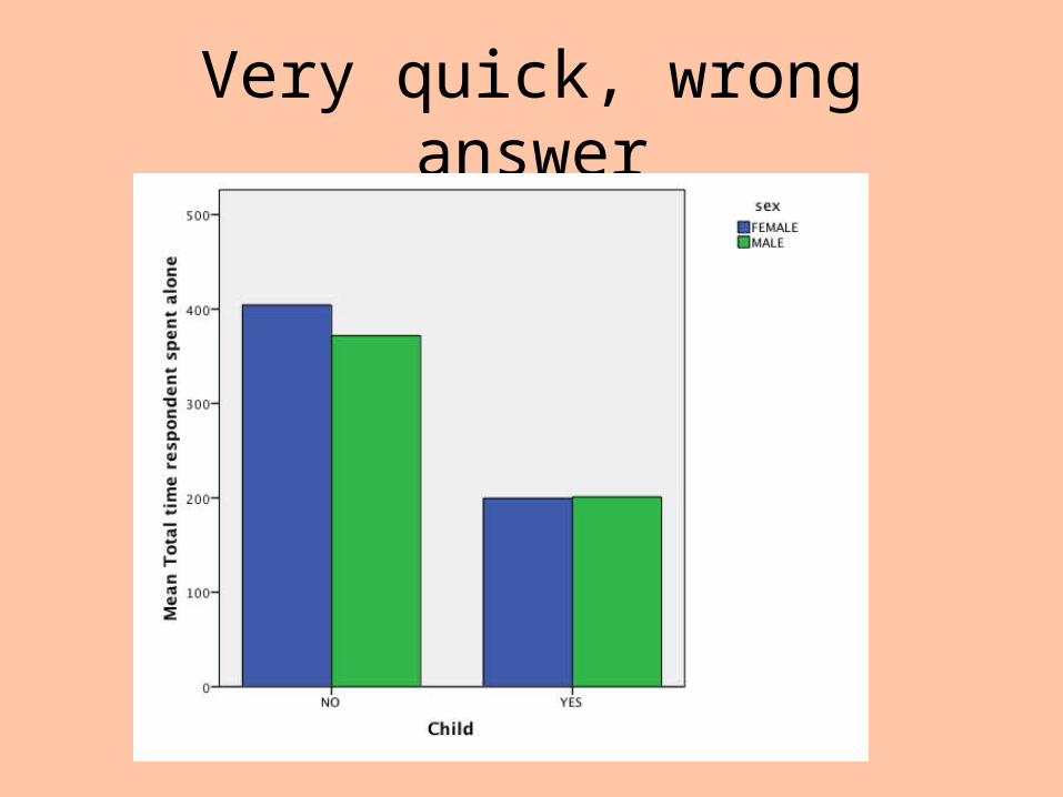
Very quick, wrong answer

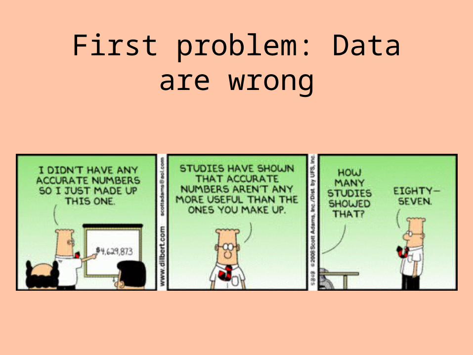
First problem: Data are wrong

Know your data. Know your data.

I said it twice because it was important.

Get to intimately know your data before you do ANYTHING.

American Time Use Survey

• Conducted by U.S. Census Bureau• Study of how a nationally representative

sample of Americans spend their time

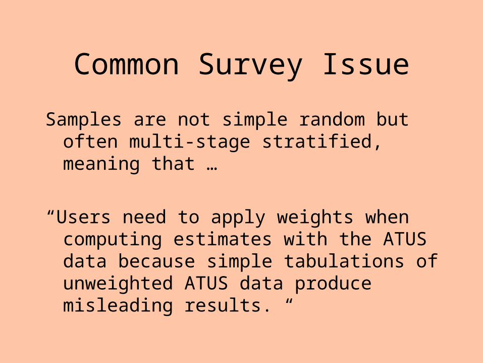
Common Survey Issue

Samples are not simple random but often multi-stage stratified, meaning that …

“Users need to apply weights when computing estimates with the ATUS data because simple tabulations of unweighted ATUS data produce misleading results. “

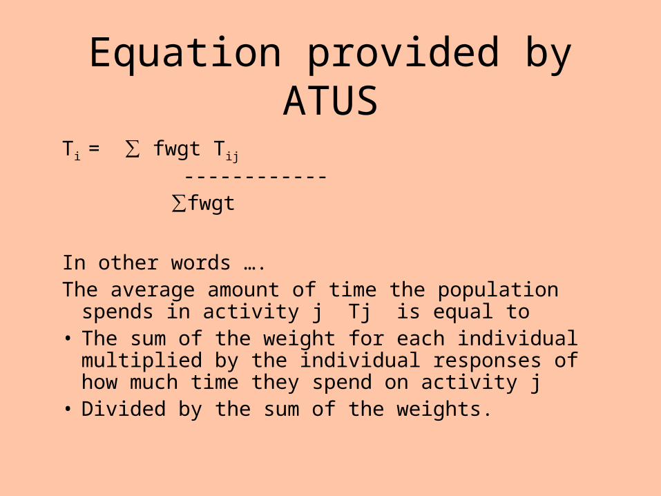
Equation provided by ATUS

Ti = ∑ fwgt Tij ------------ ∑fwgt

In other words …. The average amount of time the population spends in activity j

Tj is equal to • The sum of the weight for each individual multiplied by the

individual responses of how much time they spend on activity j

• Divided by the sum of the weights.

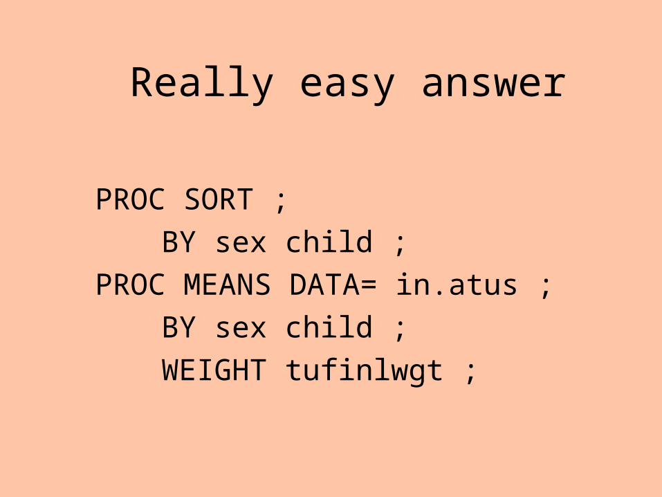
Really easy answer

PROC SORT ;

BY sex child ;

PROC MEANS DATA= in.atus ;

BY sex child ;

WEIGHT tufinlwgt ;

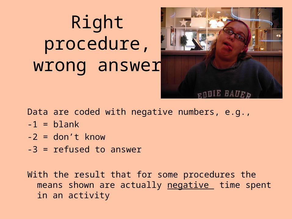
Right procedure, wrong answer

Data are coded with negative numbers, e.g.,

-1 = blank

-2 = don’t know

-3 = refused to answer

With the result that for some procedures the means shown are actually negative time spent in an activity

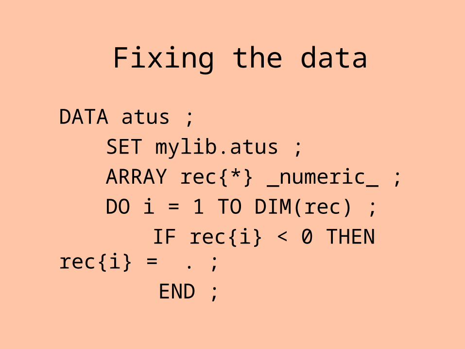
Fixing the data

DATA atus ;

SET mylib.atus ;

ARRAY rec{*} _numeric_ ;

DO i = 1 TO DIM(rec) ;

IF rec{i} < 0 THEN rec{i} = . ;

END ;

How this impacts output# of minutes per day aloneWith and without weights

Child at Home

Unweighted

Mean

Weighted

Mean

Female NO 404 347

YES 199 207

Male NO 372 324

YES 201 205

Generalizing to the Population

The Problem

I would like to get an estimate of the population values.

•How many children are in the average household?

•How many hours does the average employed person work?

A bigger problem

It is not acceptable to just calculate means and frequencies, not even weighted for percent of the population, because I do not have a random sample. My sample was stratified by gender and education.

Some common “messy data” examples

• Small, medium and large hospitals in rural and urban areas

• Students selected within classroms in high- , low- and average- performing schools

Data requiring special handling

• Cluster samples - subjects are not sampled individually, e.g., classrooms or hospitals are selected and then every person within that group is sampled.

• Non-proportional stratified samples - a fixed number is selected from, e.g., each ethnic group

PROC SURVEYMEANS DATA=in.atus40 TOTAL = strata_count ;

WEIGHT samplingweight ;

STRATA sex educ ;

VAR hrsworked numchildren ;

SAS PROCEDURE FOR A STRATIFIED SAMPLE

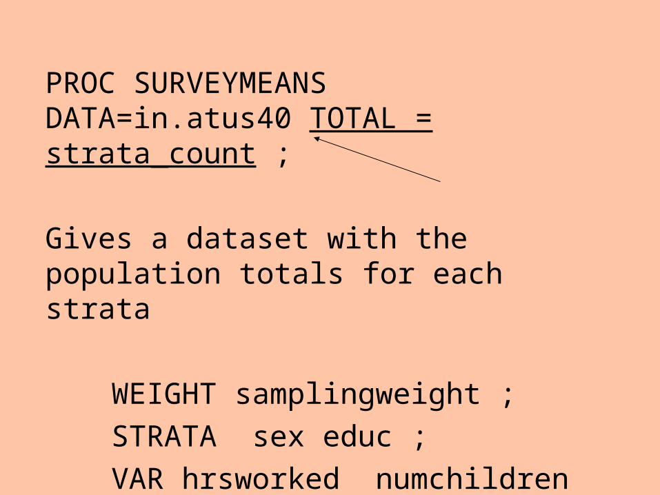
PROC SURVEYMEANS DATA=in.atus40 TOTAL = strata_count ;

Gives a dataset with the population totals for each strata

WEIGHT samplingweight ;

STRATA sex educ ;

VAR hrsworked numchildren ;

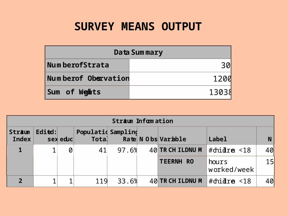
Data Summary

Number of Strata 30

Number of Observations 1200

Sum of Weights 13038

Stratum Information

Stratum Index

Edited: sex educ

Population Total

Sampling Rate N Obs Variable Label N

TRCHILDNUM #children <18 40 1 1 0 41 97.6% 40

TEERNHRO hours worked/week

15

2 1 1 119 33.6% 40 TRCHILDNUM #children <18 40

SURVEY MEANS OUTPUT

Surveymean Output

Statistics

Variable Label N Mean

Std Error of

Mean 95% CL for Mean

TRCHILDNUM #children <18 1200 0.988551 0.056994 0.8767287 1.1003729

TEERNHRO hours worked/week 247 34.630187 0.867781 32.9198281 36.3405450

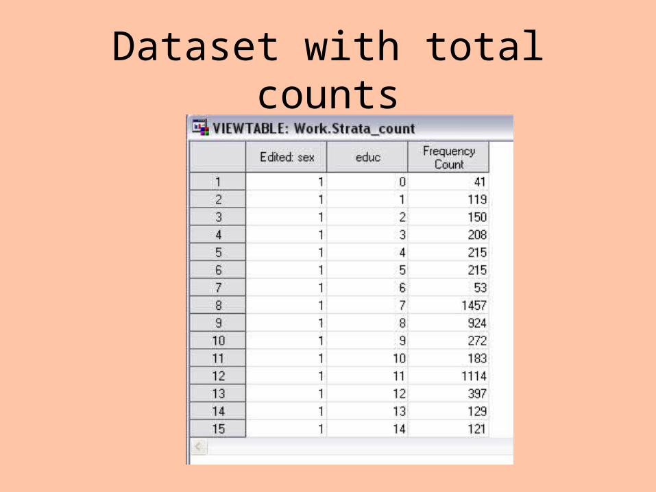
Dataset with total counts

Answers Price ListAnswers Price List

Answers $1

Answers, Correct $100

Answers, Requiring Thought -- $1,000

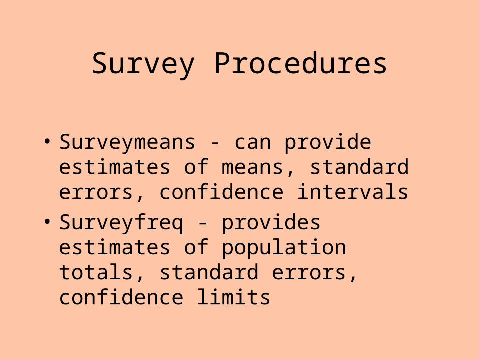
Survey Procedures

• Surveymeans - can provide estimates of means, standard errors, confidence intervals

• Surveyfreq - provides estimates of population totals, standard errors, confidence limits

And now for something completely different …

2. Using SAS Enterprise Guide to analyze target market survey data in the hour before your meeting

It’s not always rocket science

There may be a tendency to use the most sophisticated statistical techniques we can find when what the customer really wants is a bar chart

Customer Need

Our target market is Native Americans with chronic illness in the Great Plains region. We want to know how people get most of their information so that we can develop a marketing strategy.

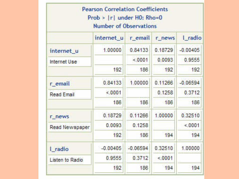
Questions

1. How often do people read the newspaper versus use the Internet?

2. Is it the same people who are using a lot of media, e.g. email, radio, Internet, or do different people use different sources of information?

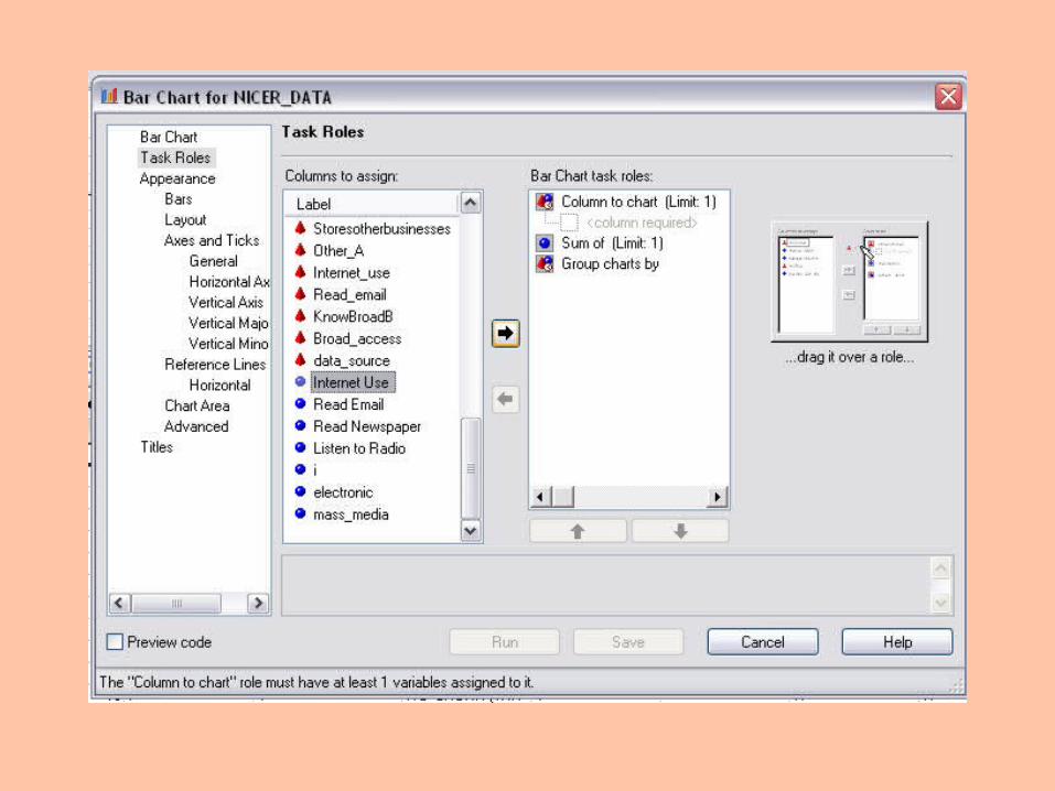
Creating Enterprise Graphs

1. Double-click on SAS dataset to open2. Select Graph > Bar Chart > Colored Bars3. Select Task Roles4. Click on Internet_Use5. Select Analysis Variable

Repeat steps for second chart for newspaper readership

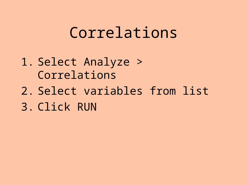
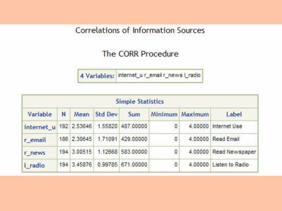
Correlations

1. Select Analyze > Correlations

2. Select variables from list

3. Click RUN

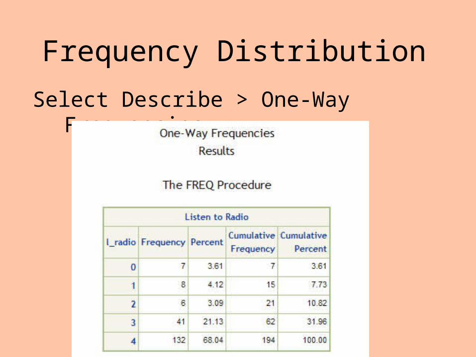
Frequency Distribution

Select Describe > One-Way Frequencies

Recommendations

• Create a website and an email list to contact potential customers on the reservations

• Advertise on the radio and in the newspaper

That will be $4,000, please.

Nice theory, but does it work?

3. Evaluating program effectiveness

We changed something. Did it work ?

A two-day staff training program was offered.

A pre-test was given before training occurred and at the conclusion of training.

The test consisted of multiple choice questions and case studies.

Just for fun ….

I decided to do the whole project using only two procedures,

PROC CORR and PROC GLM

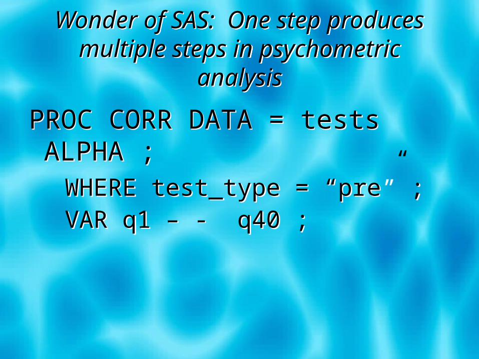
Wonder of SAS: One step produces multiple steps in psychometric analysis

Wonder of SAS: One step produces multiple steps in psychometric analysis

PROC CORR DATA = tests ALPHA ;WHERE test_type = “pre” ;VAR q1 – - q40 ;

PROC CORR DATA = tests ALPHA ;WHERE test_type = “pre” ;VAR q1 – - q40 ;

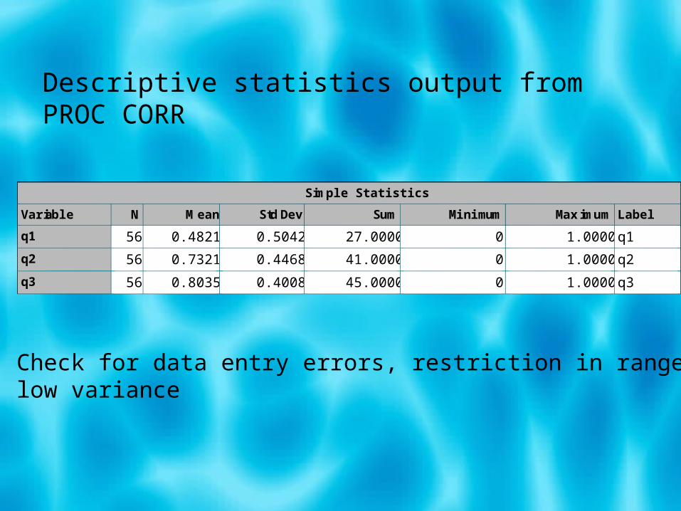
Simple Statistics

Variable N Mean Std Dev Sum Minimum Maximum Label

q1 56 0.48214 0.50420 27.00000 0 1.00000 q1

q2 56 0.73214 0.44685 41.00000 0 1.00000 q2

q3 56 0.80357 0.40089 45.00000 0 1.00000 q3

Descriptive statistics output from PROC CORR

Check for data entry errors, restriction in range,low variance

My alpha is not very good

and I am sad

My alpha is not very good

and I am sad

Cronbach Coefficient Alpha

Variables Alpha

Raw 0.670499

Standardized 0.715271

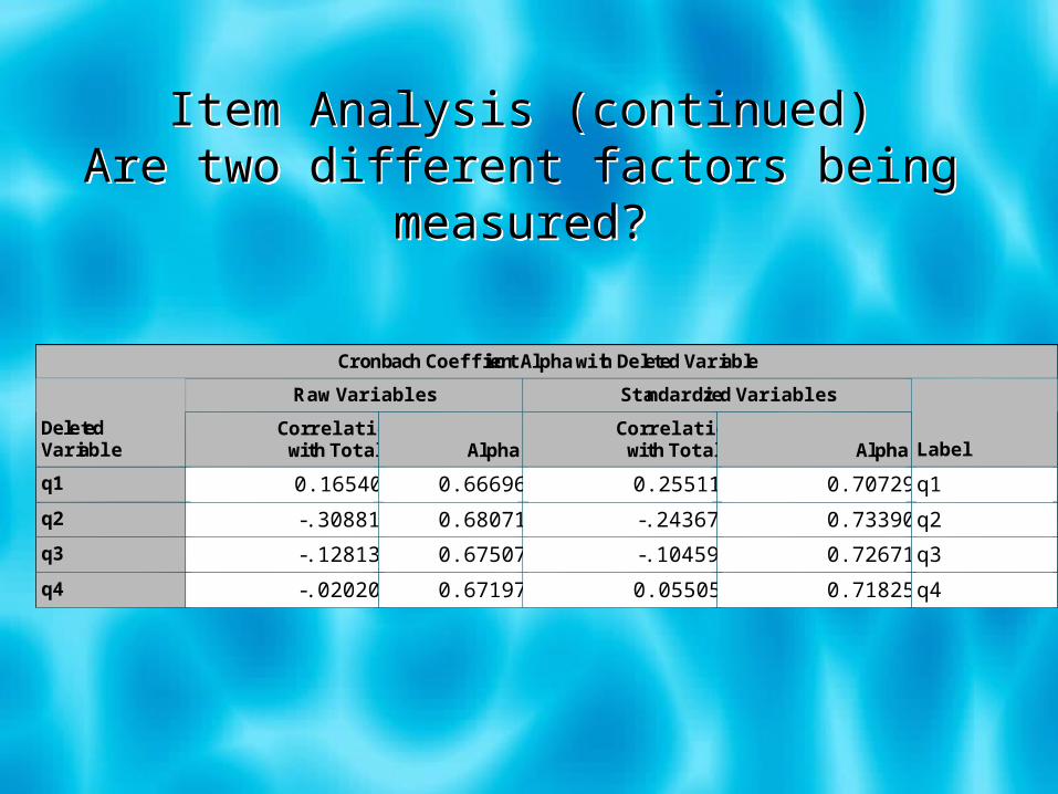
Item Analysis (continued)Are two different factors being measured?

Item Analysis (continued)Are two different factors being measured?

Cronbach Coefficient Alpha with Deleted Variable

Raw Variables Standardized Variables

Deleted Variable

Correlation with Total Alpha

Correlation with Total Alpha Label

q1 0.165402 0.666968 0.255112 0.707299 q1

q2 -.308810 0.680713 -.243679 0.733907 q2

q3 -.128138 0.675074 -.104595 0.726719 q3

q4 -.020201 0.671974 0.055058 0.718250 q4

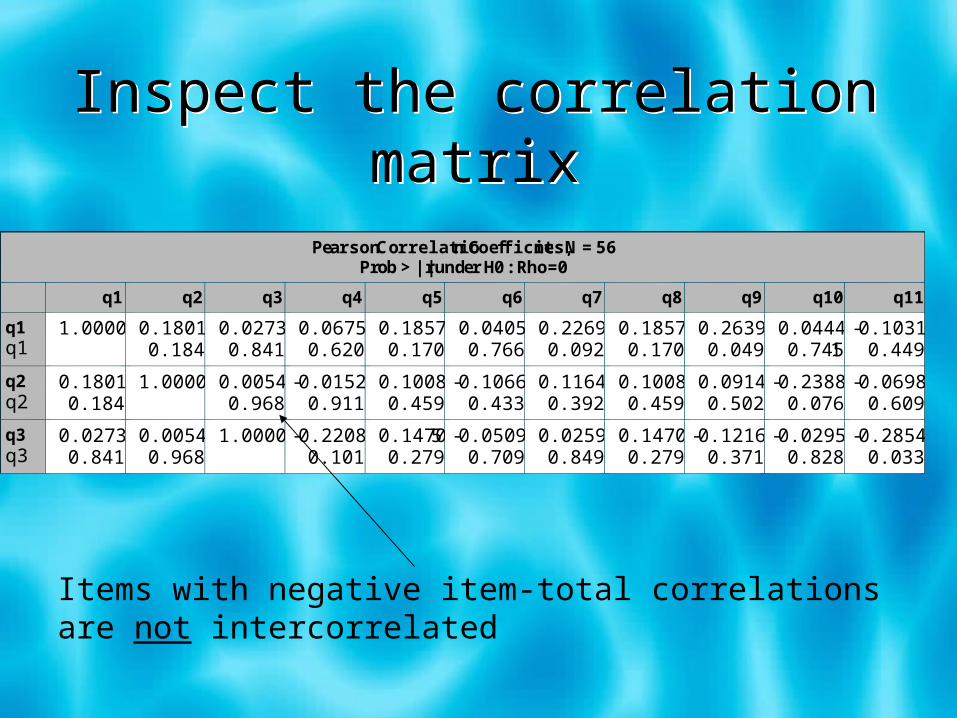
Inspect the correlation matrix

Inspect the correlation matrix

Pearson Correlation Coefficients, N = 56 Prob > |r| under H0: Rho=0

q1 q2 q3 q4 q5 q6 q7 q8 q9 q10 q11

q1 q1

1.00000

0.18013 0.1840

0.02731 0.8417

0.06754 0.6209

0.18570 0.1706

0.04052 0.7668

0.22696 0.0925

0.18570 0.1706

0.26395 0.0493

0.04443 0.7451

-0.10316 0.4493

q2 q2

0.18013 0.1840

1.00000

0.00544 0.9683

-0.01524 0.9112

0.10088 0.4594

-0.10669 0.4339

0.11641 0.3929

0.10088 0.4594

0.09141 0.5028

-0.23885 0.0763

-0.06984 0.6090

q3 q3

0.02731 0.8417

0.00544 0.9683

1.00000

-0.22085 0.1019

0.14705 0.2795

-0.05096 0.7091

0.02595 0.8494

0.14705 0.2795

-0.12161 0.3719

-0.02958 0.8287

-0.28545 0.0330

Items with negative item-total correlationsare not intercorrelated

The General Linear Model

The General Linear Model

It really is general.

You may now jump for joy at this obvious revelation.

It really is general.

You may now jump for joy at this obvious revelation.

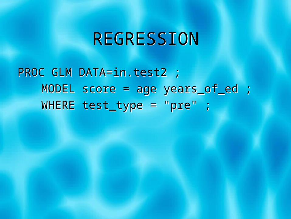
REGRESSIONREGRESSION

PROC GLM DATA=in.test2 ;

MODEL score = age years_of_ed ;

WHERE test_type = "pre" ;

PROC GLM DATA=in.test2 ;

MODEL score = age years_of_ed ;

WHERE test_type = "pre" ;

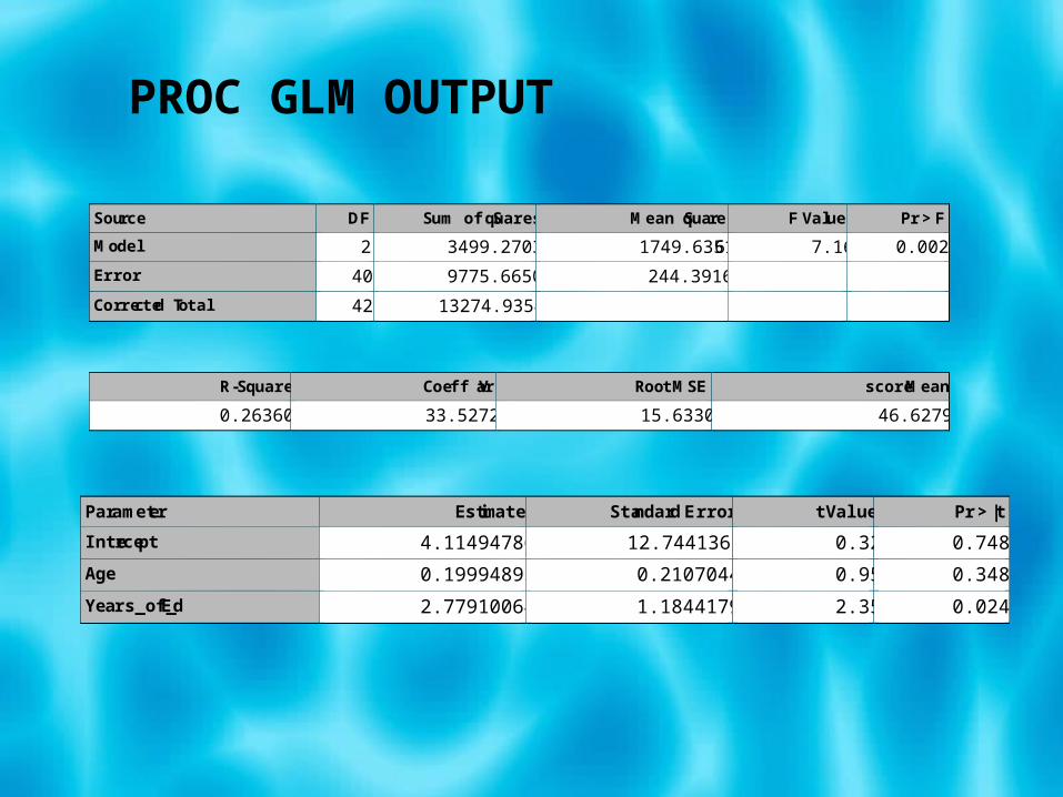
Source DF Sum of Squares Mean Square F Value Pr > F

Model 2 3499.27032 1749.63516 7.16 0.0022

Error 40 9775.66508 244.39163

Corrected Total 42 13274.93540

R-Square Coeff Var Root MSE score Mean

0.263600 33.52720 15.63303 46.62791

Parameter Estimate Standard Error t Value Pr > |t|

Intercept 4.114947869 12.74413685 0.32 0.7485

Age 0.199948936 0.21070443 0.95 0.3483

Years_of_Ed 2.779100645 1.18441794 2.35 0.0240

PROC GLM OUTPUT

2 x 2 Analysis of Variance 2 x 2 Analysis of Variance

PROC GLM DATA=in.test2 ;

CLASS disability job; MODEL score = disability job

disability*job ;

WHERE test_type = "pre" ;

PROC GLM DATA=in.test2 ;

CLASS disability job; MODEL score = disability job

disability*job ;

WHERE test_type = "pre" ;

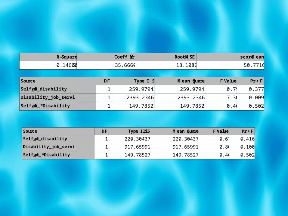
R-Square Coeff Var Root MSE score Mean

0.146002 35.66606 18.10823 50.77160

Source DF Type I SS Mean Square F Value Pr > F

Self_fam_disability 1 259.979424 259.979424 0.79 0.3775

Disability_job_servi 1 2393.234665 2393.234665 7.30 0.0094

Self_fam_*Disability 1 149.785278 149.785278 0.46 0.5022

Source DF Type III SS Mean Square F Value Pr > F

Self_fam_disability 1 220.3043773 220.3043773 0.67 0.4163

Disability_job_servi 1 917.6599111 917.6599111 2.80 0.1006

Self_fam_*Disability 1 149.7852784 149.7852784 0.46 0.5022

Repeated Measures ANOVARepeated Measures ANOVA

Uh - maybe someone should have mentioned this …..

Uh - maybe someone should have mentioned this …..

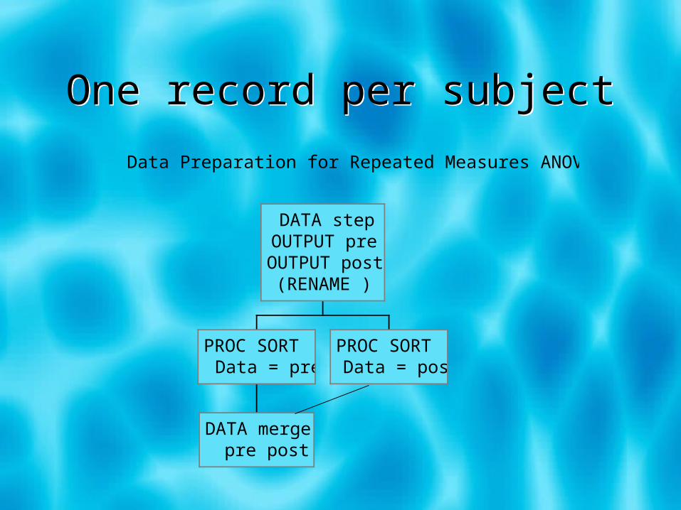
One record per subjectOne record per subject

Data Preparation for Repeated Measures ANOVA

DATA mergepre post

PROC SORTData = pre

PROC SORTData = post

DATA stepOUTPUT preOUTPUT post(RENAME )

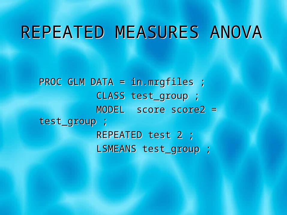
REPEATED MEASURES ANOVAREPEATED MEASURES ANOVA

PROC GLM DATA = in.mrgfiles ;

CLASS test_group ;

MODEL score score2 = test_group ;

REPEATED test 2 ;

LSMEANS test_group ;

PROC GLM DATA = in.mrgfiles ;

CLASS test_group ;

MODEL score score2 = test_group ;

REPEATED test 2 ;

LSMEANS test_group ;

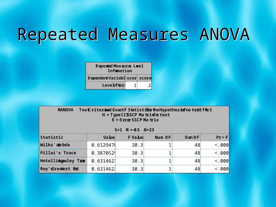
Repeated Measures ANOVARepeated Measures ANOVA

MANOVA Test Criteria and Exact F Statistics for the Hypothesis of no test Effect H = Type III SSCP Matrix for test

E = Error SSCP Matrix

S=1 M=-0.5 N=23

Statistic Value F Value Num DF Den DF Pr > F

Wilks' Lambda 0.61294702 30.31 1 48 <.0001

Pillai's Trace 0.38705298 30.31 1 48 <.0001

Hotelling-Lawley Tra ce 0.63146237 30.31 1 48 <.0001

Roy's Greatest Root 0.63146237 30.31 1 48 <.0001

Repeated Measures Level Information

Dependent Variable score score2

Level of test 1 2

Repeated Measures ANOVARepeated Measures ANOVA

Source DF Type III SS Mean Square F Value Pr > F

test 1 3716.740741 3716.740741 30.31 <.0001

test*test_group 1 2787.851852 2787.851852 22.74 <.0001

Error(test) 48 5885.925926 122.623457

LSMEANS OUTPUTLSMEANS OUTPUT

test_group score LSMEAN score2 LSMEAN

COMPA RISON 55.2222437 57.6700577

TRAINED 44.6864949 67.4265126

CONCLUSIONS

SAS has made it possible to obtain output of statistical procedures without ever needing to understand the underlying assumptions. This is a mixed blessing.

Enterprise Guide makes statistics accessible to a wider audience . This is a good thing.

The best statistical analysis is not the one that the fewest people can understand but that the most people can understand.