jukka pieskä risk factor based investing case: msci...
TRANSCRIPT
OULU BUSINESS SCHOOL
Jukka Pieskä
RISK FACTOR BASED INVESTING –
CASE: MSCI RISK FACTOR INDICES
Master’s thesis
Finance
December 2015
UNIVERSITY OF OULU ABSTRACT OF THE MASTER’S THESIS
Oulu Business School
Unit
Department of Finance
Author
Pieskä Jukka Supervisor
Kahra H. Professor
Title
Risk Factor Based Investing - Case: MSCI Risk Factor Indices
Subject
Finance Type of the degree
Master of Science Time of publication
December 2015 Number of pages
54
Abstract
The aim of this thesis is to study risk factor based investing and test how well MSCI constructs
their risk factor based indices. Risk factor based investing has gained a lot of media exposure
in the recent years and “Smart Beta” products are becoming more popular. Blackrock
estimated that there are more than 700 exchange traded products available and they have over
$ 529 billion in assets under management. Risk factor investing aims to harvest the risk
premia associated with factors like size, momentum and value.
I tested whether MSCI is able to provide higher Sharpe ratios for higher risk exposure indices
and how much they deviated from the parent index of MSCI World. I used the Ledoit & Wolf
bootstrap inference test to find out whether the Sharpe ratios of high exposure and high
capacity indices differ from each other. Furthermore, I tested how well the Fama & French
Three Factor-model with the addition of Carhart momentum factor could explain the returns
of MSCI’s risk factor indices. I also constructed different risk factor portfolios using risk-
parity methods to see whether it is possible to enhance the returns of risk factor indices by
combining them.
The main results and conclusions of this thesis were that risk factor investing can provide
excess returns. These excess returns are readily available by investing in MSCI’s risk factor
indices. Another key finding was that by utilizing risk-parity methods an investor can achieve
excess returns over an equally weighted risk factor portfolio and over the MSCI’s own
Diversified Mix index. Furthermore, even though MSCI is the world leader in index creation,
their way of creating indices doesn’t seem to be very efficient and it would be beneficial to
analyse other index providers, too.
The data used in this thesis were gathered from “MSCI’s end of day index data search”. The
data consists of six risk factor indices from developed countries. The price data ranged from
November 1998 to August 2015. For the Ledoit & Wolf test I gathered four high capacity
indices and four high exposure indices from the same time period. The proxies for academic
factors were provided by Kenneth French on his website.
Keywords
Smart Beta, Fama & French Three Factor-model, Index Provider & Risk-Parity
Additional information

CONTENTS
1 INTRODUCTION............................................................................................... 5
1.1 Background ................................................................................................... 5
1.2 Data and Results ........................................................................................... 6
1.3 Relationship with prior research ................................................................. 6
1.4 Structure of the thesis ................................................................................... 7
2 PORTFOLIO MANAGEMENT ....................................................................... 8
2.1 Brief history ................................................................................................... 8
2.2 Active and Passive Management ............................................................... 10
2.3 The Cost of Active Investing ...................................................................... 12
3 FACTOR INVESTING .................................................................................... 13
3.1 What is a factor ........................................................................................... 16
3.2 Known factors ............................................................................................. 17
4 HIGH EXPOSURE VS. HIGH CAPACITY .................................................. 20
4.1 Factor exposure ........................................................................................... 21
4.2 Investability ................................................................................................. 22
4.3 Investability vs. exposure ........................................................................... 23
4.4 Pástor & Stambaugh liquidity factor ........................................................ 24
4.5 MSCI as an index provider ........................................................................ 24
5 METHODOLOGY ........................................................................................... 26
5.1 Ledoit & Wolf time-series bootstrap confidence interval ....................... 26
5.2 Fama & French three-factor model and Carhart momentum factor .... 27
5.3 Risk parity based portfolio construction .................................................. 31
5.4 Data collection ............................................................................................. 33
6 RESULTS .......................................................................................................... 36
6.1 High exposure vs. high capacity risk-factor indices ................................ 36

6.2 Fama & French regressions ....................................................................... 38
6.3 Risk-parity portfolios.................................................................................. 42
7 CONCLUSION ................................................................................................. 47
REFERENCES ......................................................................................................... 50
TABLES AND FIGURES ....................................................................................... 54
5
1 INTRODUCTION
Traditional market-cap-weighted funds provide exposure to market risk, also known
as beta. Pure index investors encourage us to simply “own the market” with plain-
vanilla cap-weighted funds. But finance researchers have identified other sources of
risk and return over the years. The Fama & French (1993) three-factor model suggests
that a bias toward smaller firms and toward the value side of the style spectrum could
improve performance. The Carhart (1997) model adds momentum as a fourth factor.
1.1 Background
These risk factors are widely acknowledged amongst the finance research industry and
more factors are discovered every year. My thesis will look into “Morgan Stanley
Capital International” (MSCI) factor indices and test if high exposure indices provide
higher risk-adjusted returns than high capacity indices. I will also conduct a test
between different portfolio optimization methods and test how well these most well-
known factors can explain the performance of these factor-index portfolios.
Furthermore I will construct simple portfolios to represent each single factors and I
will test how much of the single factor portfolios return can be explained by the Fama
& French-Carhart model.
Andrew Ang and Thierry Roncalli have inspired me with their papers most. They have
found that factors do exist and they do offer high returns in the long run. There is only
quite little academic research conducted in last years but there is a plethora of industry
papers and I have been able to use the industry papers to motivate my thesis. My data
is from MSCI and I have found MSCI’s research papers very useful when trying to
understand their way of creating factor tilts. Factor investing has been a hot topic since
2010 and it is becoming more and more popular. According to Blackrock, in December
2014 there were more than 700 smart beta exchange traded products comprising of $
529 billion in assets under management (Shores, 2015). Funds and ETF’s exploiting
risk factors are popping up weekly and the industry is educating the investors to use
these premiums. It has been argued by Ang (2013) that the hype around factor
investing has already made the size-factor disappear.
6
1.2 Data and Results
I have gathered monthly returns data since November 1998 until September 2015 from
MSCI database. This data spans across the most well-known factors of size, value,
momentum, quality, high dividend yield and low volatility. I have both high capacity
and high exposure counterparts for value, quality, minimum volatility and momentum
factors.
The main results and conclusions of this thesis were that risk factor investing can
provide excess returns. These excess returns are readily available by investing in
MSCI’s risk factor indices. Another key finding was that by utilizing risk-parity
methods an investor can achieve excess returns over an equally weighted risk factor
portfolio and over the MSCI’s own Diversified Mix index. Furthermore, even though
MSCI is the world leader in index creation, their way of creating indices doesn’t seem
to be very efficient and it would be wise to analyse other index providers too.
1.3 Relationship with prior research
Risk factors have been said to come and go. Andrew Ang (2013) implied in his paper
that for example the risk factor premium associated with size has been diminished from
the market. My thesis will test if size has still had significant loadings in explaining
the returns of international stock returns.
In addition to Ang’s findings about the size premium, Fama and French (2012) also
found that size had no explanatory power in their sample period of international
returns. Their sample period was from November 1989 to March 2011. However, my
sample period starts and ends later so the results might differ. Fama and French also
indicated that there are significant premiums for value and momentum factors.
Thierry Roncalli (2014) indicated that the value factor has been able to provide
positive relative returns in developed markets. Also the size factor has been producing
excess returns in the US but not in other developed countries.

7
Even the results of academic researchers differ from each other. This is mainly due to
differences in data. My data is also different from any prior research and I will test
how well these most well known risk factors can explain my data.
1.4 Structure of the thesis
In chapter two I will go through the brief history of portfolio management and focus
on the main theories and the differences between active and passive portfolio
management. Then, in chapter three I will explain the basics of factor investing and
familiarise you with the most well-known factors. In chapter four I will concentrate on
MSCI’s way of creating high capacity and high exposure risk factor indices. Chapter
five delivers the methodology and the theories behind the testing phase and also the
main risk-parity methods used. I will also explain the data gathering and manipulation
in more detail. Chapter six will highlight the most important results divided in three
sections based on the testing methods. Finally chapter seven concludes.
8
2 PORTFOLIO MANAGEMENT
Portfolio management industry can be divided in two categories. Active portfolio
management aims to achieve higher returns than its benchmark index. In other words
it tries to beat the market in its own investment universe. The other category is passive
portfolio management that aims to capture the returns of benchmark indices as closely
as possible. Today a third category has been said to have emerged called “smart beta”
or risk factor based investing. Risk factor based investing aims to capture rewards for
taking the risks associated with known risk factors. However, they aim to do this
systematically to reduce the costs of active management. In a sense smart beta category
aims to capture the best sides of both active and passive portfolio management.
2.1 Brief history
Hannu Kahra (2015) has presented the short history of portfolio management in his
report to Finnish Centre for Pensions. He has followed Mark Rubinstein’s’ (2006)
example by dividing the development of finance theory in three stages:
1. Era of antique: before 1950’s,
2. Era of classical theory: 1950’s until 1980 and
3. Era of modern theory: after 1980.
Before year 1950, the practice and theory of finance were only a compilation of
investment related anecdotes. Harry Markowitz’s’ (1952) doctoral thesis about
portfolio selection is considered as the corner stone of systematic finance theory. He
offers a normative advice regarding the optimal portfolio construction when the
investor is interested only about the expected return and variance of the portfolio.
The era of classical theory began with theories such as capital asset pricing model
(CAPM), random walk-theory and the efficient market hypothesis (EMH). The
classical theory has its foundations in stating that market prices reflect all the relevant
information about its fundamental factors. It is intuitively clear that information is
efficiently gathered and used because information is valuable. The efficient market
9
hypothesis remains a cornerstone of the modern finance theory. John Cochrane (2007)
implies that the theory of efficient markets launched the classical era and formed the
investment discussion into a recognized science. The origin of finance shifted from
accounting to economics.
Cochrane (2011) states that the efficiency of the markets gets a new interpretation in
modern finance theory, but the efficient markets mark the constraints that all investors
should appreciate. There is no free lunch because information gathering is highly
competed in the investment markets. Cochranes article “new facts in finance” (1999)
expands our view of the mechanism through which the markets offer compensation
for accepting the risks and understanding the mechanism of the risk factors behind
premiums.
In the classical era theory the CAPM offers a good measure for risk and also a good
explanation to the question why different asset classes (equities, bonds, mutual funds
and different strategies) offer higher average returns than others. In the model the risk
premium offered by the market portfolio is the only source of risk and beta indicates
the exposure to this risk. This implies that an asset class can achieve higher returns
only by having higher beta or in other words higher risk. The CAPM was soon
followed by Arbitrage Pricing Theory (APT). The APT applies more risk factors in
addition to the market risk and states that investors get higher returns by accepting the
risk that is implicitly related to risk factors. Fama and French (1993) apply additional
factors to this model. They use SMB (small minus big) and HML (high minus low)
factors which take advantage of the size premium and value premium. Later Carhart
(1997) added the momentum factor to complement the model.
10
2.2 Active and Passive Management
The debate between active and passive management styles has been ongoing since the
inception of John Bogle’s first index investment trust. The Vanguard 500 Index Fund
was the first passive investment device that mimics the Standard and Poor's 500 index.
Active management style has been the dominant style for ages but passive is winning
grounds to date.
Prior research by French (2008) showed that active management is a zero-sum-game,
meaning that the aggregate of active fund returns equals the market return. When the
active fund charges its fees it results in an underperformance of the aggregate active
funds by the amount of fees charged. Even though, it has been shown that an average
active fund manager earns positive alpha before costs but he’s alpha cannot quite cover
the costs of active management.
The efficiency of the markets is in the core of active versus passive debate. Grossman
and Stiglitz (1980) argued that, in a world of costly information, informed traders must
earn an excess return or they will have no incentive to gather and analyze information
to make prices more efficient. If we lived in a world of semi-strong form of efficiency
all investors would choose passive over active management. These two findings imply
that markets need to be “mostly, but not completely efficient.” Even though active
management is a zero-sum-game, active management as a whole is definitely not. By
making markets more efficient, active management improves capital allocation, and
thereby economic efficiency and growth, resulting in greater aggregate wealth for
society as a whole.
Burton Malkiel (2003) wrote a defense for indexing after multiple papers had attacked
the efficient market hypothesis. He indicated in his paper that indexing can be justified
even if markets are less than fully efficient. Indexing is a sensible strategy because our
security markets appear to be remarkably efficient in digesting and adjusting to new
information. When information arises about individual stocks or about the market as a
whole, that information is generally reflected in market prices without delay. (Malkiel
2003:1) This is the essence of EMH. Malkiel also referred to active management as a
zero-sum game: if one investor achieves above average returns there is bound to be
11
another investor who receives below average returns. He indicated that after costs and
expenses active management as aggregate produces negative excess returns. He also
noted that passive management has other benefits than the ones explained above.
Passive management tends to minimize taxes and turnover. By minimizing turnover
trading costs like brokerage costs and ask-bid spread costs are also minimized. When
it comes to the statistical findings of prior research, Malkiel noted that the Vanguard
Index Fund has beaten 71 % of all US equity mutual funds after expenses (1991-2001).
Even during the US stock market crash of 2001, the index fund outperformed more
than 50 % of the active funds. Furthermore, similar findings from bonds are also
recorded. Even though research on active management and asset pricing suggests that
asset prices can be predictable and certain anomalies exist, professional active
management industry hasn’t been able to achieve abnormal risk-adjusted returns
persistently. Over long periods, passive management outperforms active management.
William Sharpe (1991) introduced an arithmetic formula in his paper against active
management. Based on simple rules of arithmetic’s he could prove that passive
outperforms active at all times. His two assertions stated that before costs, the return
on the average actively managed dollar will equal the return on the average passively
managed dollar. Thus after costs, the return on the average actively managed dollar
will be less than the return on the average passively managed dollar. Intuitively the
weighted average of passive portfolio returns equals market returns because passive
portfolios replicate market portfolios. From this follows that if active and passive
portfolios combined result in a market portfolio, then active portfolio must also
generate market return.
His second assertion can be proved by the fact that active management requires higher
fees and costs to function than passive management and thus active net returns are
inferior to passive net returns. Why then do sensible investment professionals continue
to make statements pro active management? Sharpe finds three main reasons.
Firstly the passive managers in question may not be truly passive, as some index fund
managers “sample” the market of choice, rather than hold all the stocks. Secondly,
active managers may not actually be that active. Closet indexers and certain buy and
hold strategies are closer to passive than active. Also, in research only professional or
12
institutional managers are taken into consideration and this can distort the results.
Thirdly, the summary statistics for active managers may not truly represent the
performance of the average actively managed dollar. In research the average %-
performance of managers is taken into consideration. To calculate the dollar-returns
researchers should calculate the beginning of period assets under management (AUM)
and compare performance to that.
Sharpe also noted that there is a problem with comparisons in the research in general.
Comparisons are usually made to a benchmark index that may not fully represent the
active manager’s ideas. The benchmark should be identified in advance and it should
be a feasible alternative.
2.3 The Cost of Active Investing
Kenneth French’s paper “The Cost of Active Investing” discusses the costs of active
investing. His paper answers how active management differs from passive in regard of
costs, risk profiles and portfolio diversification. The average active investor has spent
0, 67 % P.A. by chasing excess returns in the period of 1980-2006. This percentage is
used in fees paid to the active investment fund, to hedge funds and fund-of-funds and
to the stock exchanges that make investing possible. French focuses on the money
expenses but he also points out that the average investor could achieve diversification
benefits and risk reduction if he would switch to passive management.
Today factor investing applies dynamic factors that can be seen as combinations of
active and passive management. Factor indices are constructed with an active mind set
but they only charge similar fees to passive management. Maybe factor investing is
the next generation of investing.
13
3 FACTOR INVESTING
Factors have their roots in academic literature and the question of what drives stock
returns has been a constant discussion in modern finance. The most well-known and
oldest model of stock returns is the Capital Asset Pricing Model, which became a
foundation of modern financial theory. The CAPM was introduced by Jack Treynor
(1961, 1962), William Sharpe (1964), John Lintner (1965) and Jan Mossin (1966)
independently They built on the earlier work of Harry Markowitz on diversification
and modern portfolio theory. Consequently Sharpe, Markowitz and Merton Miller
jointly received the 1990 Nobel Memorial Prize in Economics for their contributions
to the field of financial economics. They stated that in CAPM, securities have only
two main drivers: systematic risk and company specific risk. Systematic risk is the risk
that comes from exposure to the market and is captured by beta, the sensitivity of a
security’s return to the market. Since systematic risk is something that cannot be
diversified away, investors are compensated with returns for bearing this risk. So the
expected return to any stock could be viewed as a function of its beta to the market.
Later, Ross (1976) proposed a different theory of what drives stock returns. According
to Ross’ “arbitrage pricing theory” (APT) the expected return of a financial asset can
be modeled as a function of various macroeconomic factors or theoretical market
indices. Ross has popularized the term “factor” as the models he uses are called “multi-
factor models”. Importantly, APT, unlike the CAPM, did not explicitly state what these
factors should be. Instead, the number and nature of these factor models became, and
continues to be, essentially empirical in nature.
Bender, Briand, Melas and Subramanian (2013a) explain factors as follows; “a factor
can be thought of as any characteristic relating a group of securities that is important
in explaining their returns and risks”. As noted in the early CAPM-related literature,
the market can be viewed as the first and most important equity factor. Beyond the
market factor, researchers generally look for factors that are persistent over time and
have strong explanatory power over a broad range of stocks. Bender et. al. also
discussed three key statistical criteria for factors: persistence over time, “large enough”
variability in returns relative to individual stock volatility, and application to a “broad
enough” subset of stocks within the defined universe. Since, unlike stock returns,
14
factors cannot be directly observed. Instead there remains a vigorous debate about how
to define and estimate them. Factor returns can be constructed by building factor
portfolios that mimic the target factor (as in Fama & French approach). Factor returns
can alternatively be estimated through cross-sectional regression (as in the Barra
approach). There are three main categories of factors today; macroeconomic,
statistical, and fundamental. Macroeconomic factors include measures such as
surprises in inflation, in GNP, or in the yield curve, and other measures of the macro
economy. Statistical models identify factors using statistical techniques such as
principal components analysis (PCA) where the factors are not pre-specified in
advance.
Bender et. al. (2013a) further stated that the most widely used factors are fundamental
factors. They captured stock characteristics, e.g. in which industry the stock belongs
to, what country it belongs to, valuation ratios like P/E, B/M and many different
technical indicators. They argued that the most popular factors today are value, quality,
size and momentum. In addition to these factors I will focus on minimum volatility
and high dividend yield in this thesis. These factors have been studied, tested and
proved in academic research. The latest research has provided all kinds of factors. Few
of the most unorthodox factors utilize for example the number of “Google” hits a
company receives or the number of times the company is mentioned in mainstream
media.
Andrew Ang (2013) stated that there is a lot of academic literature that shows how
certain classes of equity, debt and derivative securities have higher payoffs than the
broad market index. He showed how stocks with low Book-to-Market (value stocks)
ratios beat stocks with high Book-to-Market (growth stocks) ratios over long periods.
This phenomena is called value-growth premium. He also proved that stocks with past
high returns (winners) beat stocks with lower negative past returns (losers). This
phenomena is called Momentum.
These phenomena can be combined in portfolios having long positions in value stocks
and winners and short positions in growth stocks and losers. By combining long value
with short growth one can collect the value-growth premium with minimal market
exposure.
15
This kind of investment strategy can’t be achieved passively because the strategy
involves time-varying positions in securities which fluctuate over time. These are
called dynamic factors and the factor premiums don’t come for free. Ang (2013)
showed that while dynamic factors may beat the market over long periods of time, they
can grossly underperform the broad market index in bad times. He contemplated that
the factor risk premiums are persistent because they reward investors for bearing high
losses during bad times. This implies that factors are not appropriate for all investors
because they are risky.
Ang (2013) stressed that it is very important to notice that dynamic factors remove
market exposure. Optimally constructed value-growth portfolio removes the market
exposure and is only exposed to the returns of value stocks less the returns of growth
stocks. This applies to momentum and size factors also. In practice it is important that
factor portfolios are constructed with an equal number of stocks or equal dollars in
offsetting long and short positions. The less the short positions, the greater the
correlation of the factors with the broad market index. For example, one can find
multiple of investment products utilizing the value factor but most of these products
are constrained and can’t use shorting. This results in the fact that the main driver of
returns in these funds is the market portfolio. If shorting is applied more and more of
the market movements will be removed and the factor portfolio will end up reflecting
the difference between value and growth stocks.
The investment industry often uses the terms smart beta, alternative beta, or exotic beta
for dynamic factors. Ang uses the term “factors” because, in asset pricing theory, beta
has the strict meaning of measuring exposure to a risk factor. These risk factors
actually have a beta of one with respect to themselves. Ang pointed out that beta
measures the magnitude of the exposure to a risk factor and investors invest in factors,
not betas.
The recent popularity of Smart Beta as a defined asset class is a result of multiple
trends currently impacting the investment management industry. First, advances in
technology and communications have made fundamental analysis more easily
available. Many insights that have required subjective investment analysis can now be
captured in a more systematic way. Second, the investment industry has witnessed a
16
decade long rise in passive investing as investors seek transparency, consistency and
low fees offered by indexation. Third, the underfunded status of multiple personal
retirement accounts and pension funds has drawn investors to the benefits of passive
investing but they are not ready to give up on the allure of excess returns marketed by
active managers (Shores, 2015).
3.1 What is a factor
Factor investing is new to the market and it is in boom right now. New factors pop up
all the time and they are easy to sell under the umbrella of “smart beta”. Today there
are more than 300 factors described but only a handful has been widely accepted by
the academy. Ang (2013) stated that the four most important features of a risk factor
are;
1) Factors must be justified by academic research.
Factors should be based on an intellectual ground and only those factors that have the
strongest support from the academy should be accepted as benchmarks. Research
ought to exhibit compelling rational logic or behavioural stories or both in explaining
the existence of these risk premiums.
2) Factors ought to have exhibited significant persistent premiums.
It is important to understand why these factors have generated premiums and we
should have rational ground in believing that these premiums will persist also in the
future.
3) Factors should have historical returns data for bad times also.
These factor risk premiums mainly exist because they provide rewards for the
willingness to suffer significant losses during bad times. It is important that the data
has some data points to measure the “worst-case” scenarios for the assessment of risk-
return trade-offs and risk management. It is also important to have a reasonably long
data set from the point of view of statistical significance.
17
4) It should be possible to implement the factor strategy in liquid and easily
tradable instruments.
This fourth feature takes theory into practice by giving investability constraints. It is
important that it is possible to invest in a factor cheaply and that the investment is
liquid. It is also very important to large investors that it is possible to scale the
investment. Factor strategies involve leverage and they work best when leverage is
applied. Long-short approach is also important from the point of view of nulling the
market exposure. However it has been shown by Israel and Moskowitz (2013) that
factors still work without shorting.
3.2 Known factors
In this chapter, I will describe the most common factors in use today in detail and the
ideas behind them.
The market (MKT) factor represents the exposure to a broad market index. It is plain
vanilla cap-weighted factor that comes from owning the market. The MKT factor is
not a dynamic factor. It is simply the reward of bearing market risk, for example by
going long in a broad market index.
Ang (2013) stated that factors come and go and may even disappear. He implied that
the size effect has worked well in the past but doesn’t work anymore. Banz (1981)
discovered in his paper that small stocks outperform large stocks and the size premium
was acknowledged by the industry soon after. Banz and many other scholars found
that small stocks outperform large stocks for multiple reasons. Smaller stocks tend to
be more illiquid, less followed by analysts and they operate in riskier segments of the
economy. However, since the mid-1980’s the size premium has disappeared after
adjusting for market risk, ie. smaller stocks still have higher returns than large stocks
but not after debiting out their exposure to the market factor. Ang suggested that the
size premium has disappeared because of the creation of small stock mutual funds.
They made it possible for ordinary investors to bear size-related risks. Even though
Ang suggested that size-premium doesn’t exist anymore I will test it in this thesis. I
believe that size can still explain some of the returns of multifactor portfolios.
18
The next five factors were described by Bender et. al. (2013a). High minus low factor
uses the spread in returns between value and growth stocks. HML factor argues that
companies with high book-to-market ratios (value stocks) outperform those with low
ratios (growth stocks). It aims to capture excess returns to stocks that have low prices
relative to their fundamental value. The risk premia is commonly captured by book to
price, earnings to price, book value, sales, earnings, cash earning, net profit, dividends
and cash flow ratios.
The momentum factor reflects excess returns to stocks with stronger past performance.
WML factor is usually captured by relative returns historical alpha. It can be captured
with different time intervals with the most common being 3, 6 and 12 month intervals.
Quality (QUAL) factor aims to capture excess returns to stocks that are characterized
by stable earnings growth, low debt and other “quality” metrics. It is commonly
captured by return-on-equity, earnings stability, dividend growth stability, strength of
balance sheet, financial leverage, accounting policies, strength of management,
accruals and cash flows.
Minimum volatility (MVOL) factor aims to capture excess returns to stocks with lower
than average volatility, beta and/or idiosyncratic risk. It is commonly captured by
standard deviation (1-3-yrs), downside standard deviation, standard deviation of
idiosyncratic returns and beta.
High dividend yield (HDY) aims to capture the excess returns of stocks that have
higher than average dividend yields and it is commonly captured by dividend yield
and dividend growth.
Another interesting factor introduced by Pástor & Stambaugh (2013) is the liquidity
factor. MSCI does not use it in their methodology yet, but I believe it is an important
driver behind the differences of high exposure and high capacity indices. Furthermore,
it could be a useful factor to add into the Fama, French & Carhart model. It may be
able to explain some of the alpha and also some of the momentum factor.

19
Fama and French offer a benchmark for these factors on Kenneth Frenchs website.
These benchmark portfolios offered by Fama and French are commonly used in
academic research. There are also a plethora of other factors but they are out of scope
of this thesis.
20
4 HIGH EXPOSURE VS. HIGH CAPACITY
This chapter explains MSCI’s way of creating indices. By testing these indices I will
gain a clear view of the quality of MSCI’s work. I will clarify how much MSCI tilts
their indices or does the market still explain most of the returns. I will also test whether
the Sharpe of high exposure vs. high capacity indices are statistically significant by
utilizing the Ledoit & Wolff bootstrap test.
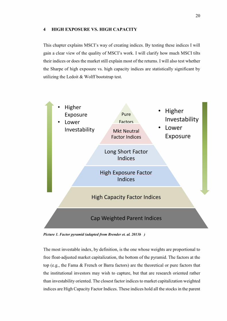
Picture 1. Factor pyramid (adapted from Brender et. al. 2013b )
The most investable index, by definition, is the one whose weights are proportional to
free float-adjusted market capitalization, the bottom of the pyramid. The factors at the
top (e.g., the Fama & French or Barra factors) are the theoretical or pure factors that
the institutional investors may wish to capture, but that are research oriented rather
than investability oriented. The closest factor indices to market capitalization weighted
indices are High Capacity Factor Indices. These indices hold all the stocks in the parent
Pure
Factors
Mkt NeutralFactor Indices
Long Short FactorIndices
High Exposure FactorIndices
High Capacity Factor Indices
Cap Weighted Parent Indices
• Higher Exposure
• Lower Investability
• Higher
Investability
• Lower Exposure
21
index but tilt the market cap weights toward the desired factor. As one moves up the
pyramid, high exposure indices hold a subset of the constituents in the parent index
and can employ more aggressive weighting mechanisms. The investor who seeks to
control active country or industry weights or exposures to other style factors can use
high exposure indices that employ optimization or systematic stock screening. High
exposure indices suits also those investors who want to limit turnover, tracking error,
or concentration. Further up the pyramid, Long/Short Factor Indices add leverage (e.g.,
150/50, 130/30) primarily to hedge out residual exposure to other factors. Finally
Market-Neutral Factor Indices are pure long/short zero investment indices that have
zero market exposure. These leveraged index categories typically employ optimization
methods.
4.1 Factor exposure
What does factor exposure actually mean? MSCI explains that factor exposure
captures the amount how much the index has the pure “non-investable” factor. They
suggest that for measuring the factor exposure investors could use different factor
models like the Fama, French & Carhart model that I use in this thesis. Alternatively
one could use the Barra factor model which incorporates over 40 data metrics
including: earnings growth, share turnover and senior debt rating to name a few. Factor
exposure is most commonly expressed as standard deviations away from the cap-
weighted average of the market. It is worth noting that these factor models typically
employ linear exposures and regressions so the exposure of an index to a factor is the
weighted average of the exposure of the constituents. Factor exposure can alternatively
be called signal strength (Bender et. al. 2013b).
Bender et. al. (2013b) also noted that it is important to control for incidental bets to
other factors. If the control fails one might get unintended exposure to other factors
and the returns might not scale up when exposure is increased.
22
4.2 Investability
According to Bender et. al. (2013b) investability can be measured by liquidity and
tradability of the index. Investability also refers to the scalability of the allocation to
an investment product that replicates the risk factor index. It can also be measured by
turnover, cost of replication and capacity. Tradability/liquidity quantifies how tradable
the portfolio is and how liquid the constituents are in the index replicating portfolio.
The metrics include days to trade a certain portion of the portfolio and days to trade
individual constituents at rebalancing and during initial construction. Turnover/cost of
replication aims to measure the turnover of the index at rebalancing which directly
affects the trading costs. The higher the turnover is, the higher the costs usually are.
Active managers commonly use measures that show how much they deviate from the
index. Few of these measures are active share and maximum strategy. Finally the
capacity measure indicates the percentage of a stocks’s free float the portfolio would
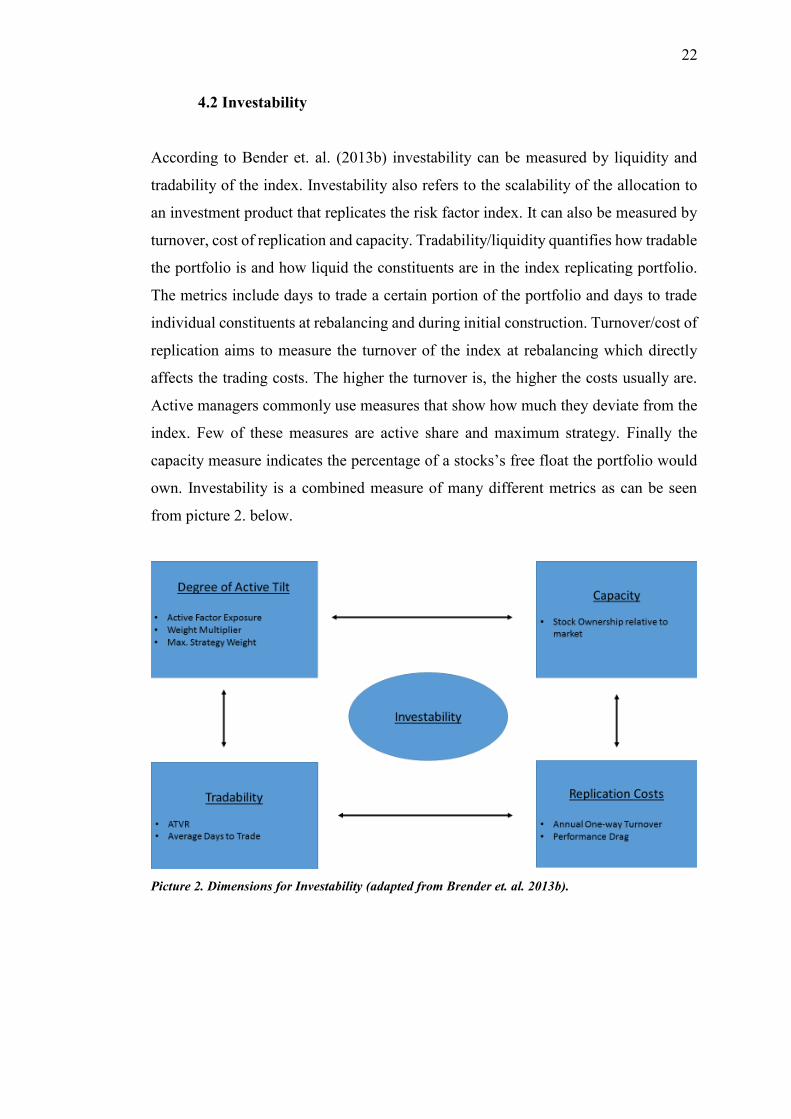
own. Investability is a combined measure of many different metrics as can be seen
from picture 2. below.
Picture 2. Dimensions for Investability (adapted from Brender et. al. 2013b).
23
4.3 Investability vs. exposure
There is an unavoidable trade-off between investability and exposure. Indices nearer
the top of the pyramid in picture 1. have higher exposures to the desired indices but
lower investability. Institutional investors must then decide what their preferences are
and where they want to be on the pyramid. For institutions it is usually important to
have low tracking error. However, when investors move up the pyramid in chase of
higher returns, tracking error usually increases at the same time. If the institution has
tracking error limits it must also limit its investments to the lower end of the pyramid.
According to Bender et. al. (2013b) higher capacity indices typically hold exposure to
a broad set of risk-factors and they are weighted with investability preferences in focus.
High exposure indices aim to mainly hold exposures to the desired factor only. This
being said the high exposure indices tend to be more concentrated and have lower
investability.
One additional insight for institutional investors is that by combining these risk factor
indices, it is possible to reduce trading costs by leveraging the benefits of natural
crossing. Reducing the trading costs can be achieved by optimization methods during
the construction of the portfolio and at each rebalancing stage. Take for example a
stock whose price has fallen over time. As the price falls, it may drop out of momentum
index but incidentally the lower price might push the stock into a value index. Now
instead of selling the stock from the momentum portfolio and buying it in the value
portfolio, the investor can just let the natural crossing reduce the trading costs. The
aim of the MSCI Diversified Mix Index is to take advantage of this phenomena.
24
4.4 Pástor & Stambaugh liquidity factor
Liquidity has been an elusive and wide concept that denotes the ability to buy or sell
large amounts quickly, at low cost and without having an effect on the price. Pástor &
Stambaugh (2013) implied that liquidity could be an important factor for asset pricing
theory. They stated that liquidity is a priced state variable and it can be used to predict
expected returns. In their minds it seems reasonable that investors require higher
expected returns on assets whose returns are more sensitive to aggregate liquidity.
They argue that portfolios that have more sensitivity to aggregate liquidity are more
likely to face margin calls and liquidations when aggregate liquidity is low. Then if
the liquidity is already low it is difficult to liquidate the portfolio in order to meet the
margin call. They concluded that adding their liquidity factor to a mean-variance
frontier constructed of the MKT, SMB, HML, MOM and risk free cash position, they
were able to increase the Sharpe ratio significantly.
As the investability decreases when moving closer to the pure academic factors, I
suspect that the liquidity also decreases. This implies that the Pástor & Stambaugh
liquidity factor might be able to predict or explain the return differences in high
exposure and high capacity indices. I will contemplate on this more in results and
conclusions.
4.5 MSCI as an index provider
MSCI is the leading index provider in the world and it has devised its own
methodology for creating these indices. I will find out if their way of creating these
risk factor indices is good by testing does higher exposure to the risk factors create
higher risk-adjusted returns compared to the high capacity indices. I will also test if
MSCI’s risk factor indices are able to create excess returns over the Fama & French
model with the addition of Carhart momentum factor. My hypothesis for this study are
below.

25
My first hypothesis is as follows:
H0: High exposure indices provide higher and statistically significant risk-adjusted
returns than high capacity indices.
H1: High exposure indices don’t provide higher and statistically significant risk-
adjusted returns than high capacity indices.
The second hypothesis is as below:
H0: MSCI risk factor indices provide statistically significant excess returns.
H1: MSCI risk factor indices don’t provide statistically significant excess returns.
In the next chapter I will go through the methods used for testing my hypothesis.
26
5 METHODOLOGY
I will conduct a series of different tests to answer at least the following questions:
1. I will test for the high exposure and high capacity indices and find out if high
exposure indices provide higher risk-adjusted returns over high capacity
indices.
2. I will utilize the Fama & French three-factor model with the addition of
Carhart momentum factor. I will run a time-series regression on my data of
monthly prices to see how well this model can explain the returns of MSCI’s
individual risk factor indices.
3. I will also explain the risk-factor indices’ returns with the parent index, MSCI
World. This will explain how much MSCI tilts their risk-factor indices away
from the parent index.
4. I will construct different risk factor-based portfolios using risk parity methods
and try to beat the MSCI Diversified Factor Mix index.
5.1 Ledoit & Wolf time-series bootstrap confidence interval
Ledoit & Wolf (Ledoit & Wolf, 2008) have designed a robust method for testing time-
series related Sharpe ratios. They imply that performance hypothesis testing with the
Sharpe ratio is not valid when returns have tails heavier than the normal distribution
or are of time series nature. Instead they use a robust inference method by constructing
a studentized time series bootstrap confidence interval for the difference of Sharpe
ratios. Then they can declare that the two Sharpe ratios are different if zero is not
included in the confidence interval.
I have collected price data of 8 different indices from MSCI for the purpose of testing
high exposure and high capacity performance. The data ranges from November 1998
to September 2015. My data has both high exposure and capacity counterparts for the
quality, minimum volatility, momentum and value factors. I will calculate the excess
mean returns, volatilities and Sharpe ratios for these indices and finally I will test if
27
the Sharpe ratios are statistically different from each other. This way I will be able to
demonstrate that is it worth it to move up in the pyramid towards the pure factor
exposures.
5.2 Fama & French three-factor model and Carhart momentum factor
Capital asset pricing-model has been a widely used and accepted model to interpret
portfolio returns in the past. After CAPM’s first introduction (Treynor 1961) to
markets there has been a lot of academic research regarding the sources of returns or
premiums. Research has shown that many anomalies question the use of CAPM as a
model that predicts future market returns. These anomalies suggest that certain
investment styles are persistently in contradiction with the expected return forecasts
provided by the CAPM. In practice investors can achieve premium (excess market
return) by investing in certain style of equities. For example if a portfolio manager
invests in these premium offering equities he can achieve higher returns than the funds
benchmark index but the excess return may not be due to alpha. CAPM can’t capture
the portfolio managers’ skill nor the active returns but suggest only that the excess
returns are due to high alpha. This is why we need models that measure exposure to
these anomalies. The answer to this problem is using multifactor-models that measure,
in addition to the market portfolio the portfolios returns correlation to certain returns
generated by these anomalies.
The best known multifactor-model is the Fama & French three factor-model (Fama &
French 1993) that measures the returns correlation with the market premium and small-
cap stock premium and the value stock premium. The Fama & French three factor
model can be phrased as follows:
rp = αp + βprM + βpSMBSMB + βpHMLHML + εp, (1)
where rp = portfolio p’s excess return, αp = portfolio p’s alpha as the models constant
term, βpM, βpSMB, βpHML = portfolio p’s beta coefficients, that measure the portfolios
exposure to different factors, rM = excess return on market, SMB = small cap stock
premium that exceeds large cap stock returns (Small Minus Big), HML = high book-
28
to-market-ratio stock returns that exceeds low book-to-market stock returns (High
Minus Low) and εp = residual as the unexpected return of the portfolio.
Fama and French (1992) studied corporate specific financial ratios effect on price
changes and they noticed that portfolios constructed of small companies and high
book-to-market companies can explain the variations of the prices. Small companies’
premium also known as the size premium is based on a finding by Banz (1981). He
stated that companies of smaller market-cap produce higher risk-adjusted returns than
larger market-cap companies. This study utilized the CAPM as its methodology.
Rosenberg, Reid and Lanstein (1985) noticed the same phenomena on stocks which
book-to-market-ratio is larger than average. Fama and French (1993) continue to refine
these findings to factors that they use together with the market factor to explain the
variations in returns. They find that these factors can explain the variations of the
returns quite well and in addition they don’t have high correlation with each other.
Fama and French (1996) present their three factor model in its most recognized form
and state that these factors explain remarkably well the anomalies found in CAPM.
Ri - Rf = αi + bi(RM-Rf) + siSMB + hiHML + εi (2)
Fama and French (1996) also find that the three factor model has some caveats. It does not
fully explain the persistence of returns on a short time period. This is why the model might
need more factors to function better. The finding that positive returns are followed by
positive returns and negative returns followed by negative returns was first done by
Jagadeesh and Titman (1993). They also noticed that a strategy that buys stocks that have
performed well in the past and sell stocks that have performed poorly in the past produces
significant abnormal returns. In other words returns that exceed the expected return
forecasted by CAPM. This phenomena is called momentum. Carhart (1997) studied the
persistence in mutual fund performance and adds the momentum factor to Fama & French
three factor-model. Momentum-factor measures the portfolios returns exposure to the
premium associated with this anomaly. Carhart finds that momentum explains a
considerable portion of the alpha of some mutual funds. This model is also called Carhart
four factor model and in can be presented as follows:
rp = αp + βprM + βpSMBSMB + βpHMLHML + βpWMLWML + εp, (3)
29
in this model the coefficients and constant terms are the same as in equation (1) but we
have added another factor βpWMLWML, in which βpWML is a beta-coefficient that
represents the exposure to the momentum-premium and WML (Winners Minus
Losers) is the return of the momentum portfolio.
Even though there are many different multifactor models that are based on regression
analysis, these afore mentioned three and four factor models are widely used amongst
academics and also industry specialists. These models are used to measure returns and
to explain the source of the returns and of course measure the alpha of the portfolio. I
will use the Carhart four factor model to measure the price data that I have gathered
from MSCI database.
The proxies for worldwide factor portfolios were available at Kenneth French’s
homepage. These international factors have been used in “Size, Value, and Momentum
in International Stock Returns” by Fama and French (2012).
The global factors and portfolios include all 23 countries in the four regions: Australia,
Austria, Belgium, Canada, Denmark, Finland, France, Germany, Greece, Hong Kong,
Ireland, Italy, Japan, Netherlands, New Zealand, Norway, Portugal, Singapore, Spain,
Switzerland, Sweden, United Kingdom and United States. The proxies are quoted in
U.S. dollars, including dividends and capital gains. The market factor is the return on
a region’s value-weighted market portfolio minus the U.S. one month T-bill rate. For
the SMB and HML factors Fama and French sorted stocks in all four regions to two
market cap and three book-to-market equity (B/M) groups. Big stocks were those in
the top 90 decile and small stocks in the bottom 10 decile. For the B/M breakpoints
they used 30th and 70th percentiles.
The 2x3 sorts on size and lagged momentum to construct WML were similar, but the
size-momentum portfolios were formed monthly. For portfolios formed at the end of
month t–1, the lagged momentum return is a stock's cumulative return for month t–12
to month t–2. The momentum breakpoints for a region are the 30th and 70th percentiles
of the lagged momentum returns of the big stocks of the region.

30
SMB is the equal-weight average of the returns on the three small stock portfolios for
the region minus the average of the returns on the three big stock portfolios.
SMB = 1/3 (Small Value + Small Neutral + Small Growth) –
1/3 (Big Value + Big Neutral + Big Growth).
HML is the equal-weight average of the returns for the two high B/M portfolios for a
region minus the average of the returns for the two low B/M portfolios.
HML = 1/2 (Small Value + Big Value) – 1/2 (Small Growth + Big Growth).
WML is the equal-weight average of the returns for the two winner portfolios for a
region minus the average of the returns for the two loser portfolios.
WML = 1/2 (Small High + Big High) – 1/2 (Small Low + Big Low).
Now it is important to notice that these factor proxies are long-short portfolios. They
are supposed to have close to zero market exposure. This is the pitfall of academic
factors. They are great for academic studies but very difficult to achieve in the
industry. Furthermore the long-short factors might not be able to explain the returns
of long-only MSCI factor-indices.
By utilizing the Fama & French three factor model with the addition of Carhart
momentum factor I will be able to estimate the quality of MSCI risk-factor indices. I
will also test how much MSCI actually tilts their risk-factor indices away from the
MSCI World parent index by running the time-series regression with MSCI World as
the explaining factor. This way I will gain valuable information about the true nature
of MSCI factor indices.
I have divided the time-series testing in three phases. In the first phase I will test
MSCI’s individual risk factor indices with the Fama & French factor model with the
addition of Carhart Momentum factor. Then I will test how much the MSCI World
index returns can explain the individual risk factor indices returns. This way I will find
out how much the MSCI risk factor indices provide exposure to the four academic

31
factors and how much have they been tilted away from the parent index. In the third
phase I have constructed different portfolios from the risk factor indices by utilizing
risk parity methods. I will test whether it is possible to beat the MSCI Diversified
Factor Mix index that has equal weights in all the six risk factor indices. I will also test
how well the Fama, French & Carhart model can explain the returns of these portfolios.
These tests will further enlighten me about the quality of MSCI risk factor indices.
The Fama, French & Carhart model is extremely used in the industry and it rests on a
solid theoretical base. Being one of the earliest multifactor model it has rooted itself
in the research. I believe that in this study it could have been useful to add more factors
to this model. One especially interesting factor is the Pástor & Stambaugh liquidity
factor. It may have been able to explain the differences in high capacity and high
exposure indices and also in the risk parity portfolios. Are the benefits of higher
exposure to a risk factor only compensation of lower liquidity?
5.3 Risk parity based portfolio construction
I will run multiple risk-parity based optimization methods on my data and I will figure
out which methods provide the best results. I will test portfolios created by minimum
variance (MV), 1/N, equal risk contribution (ERC) and systematic risk parity (SRP).
With these portfolios I will try to beat MSCI’s own Diversified Factor Mix index.
MSCI utilizes the 1/N method in constructing the Diversified Mix index (Bender,
2013b).
Maillard et.al. (2008) have good introduction to portfolio optimization methods. They
first introduced the minimum variance portfolio, which is a simple portfolio on the
Markowitz’s efficient frontier. It is also the only mean-variance frontier portfolio that
is presumed to be robust as it does not require expected returns to compute.
Unfortunately, minimum variance portfolios suffer from portfolio concentration. A
step up from minimum variance portfolios is the 1/N portfolio, which gives equal
weights to all components. It has been shown that 1/N portfolios are efficient out-of-
sample. These two above methods are simple and widely used in the industry due to
their good implementation properties. Next they introduced the ERC method, which
allocates weights so that every constituent has equal contribution to the overall risk of
32
the portfolio. The risk contribution of stock X for example is the share of total portfolio
risk that is attributable to that stock. It is computed as the product of the allocation in
stock X with its marginal contribution to risk. Marginal contribution to risk is
calculated as the change in total risk of the portfolio induced by an infinitesimal
increase in holdings of stock X. They also showed that ERC portfolios tend to lie
between minimum variance and 1/N portfolios in terms of returns. An extension of the
ERC-method was introduced by Kahra (2015). This extension is called Systematic
Risk Parity (SRP) and it allocates risk budget to each portfolio component in
proportion to its systematic risk.
I have formed 5 different portfolios from the before mentioned six factor indices by
utilizing different portfolio construction methods. The methods are chosen based on
the plausibility of the weights they offer after shorting-, leverage-, and turnover
constraints. Most common and easy to construct is the 1/N method. It simply gives
equal weights to each component in the portfolio. This naive method will also serve
as a control for the risk-parity methods. I have also constructed the minimum variance
portfolio introduced by Markowitz. Furthermore I have chosen two different risk-
parity methods from a group of 7 methods. Equal risk contribution (ERC) and
systematic risk parity (SRP) gave suitable weights, keeping in mind the investability
of the methods. When I conducted portfolio optimization for inverse volatility (IV),
inverse variance (IV2), alpha risk parity (ARP), maximum diversification (MD) and
diversified risk parity (DRP) I got weights that utilized high leverage and shorting.
After giving constraints these methods gave zero weights to multiple factors and
unproportional weights to only few factors, namely minimum volatility.
33
5.4 Data collection
I have collected my data from the “MSCI end of day” data search. I chose MSCI as
my data source because it was readily available and a large group of different
investment products use MSCI indices as their benchmarks. MSCI is widely known
reliable and respected index provider. I have monthly price data from November 1998
to September 2015. The indices that I have chosen are quoted in USD and they
represent the developed world markets. MSCI has created indices that provide factor
exposures. My data comprises of six different indices giving exposure to the size
(SMB), value (HML), momentum (WML), high dividend yield (HDY), minimum
volatility (MVOL) and quality (QUAL) factors. The risk free rate is represented by 1-
month Libor rate. From the HML, QUAL, MVOL and WML factors, I will conduct a
study of comparing Sharpe ratios between high exposure and high capacity indices.
Furthermore I will test if the Sharpe ratios are statistically different from each other by
conducting a Ledoit-Wolf-test.
The MSCI World Equal Weighted Index represents an alternative weighting scheme
to its market cap weighted parent index, the MSCI World Index. The index includes
the same constituents as its parent large and mid-cap securities from 23 Developed
Markets (DM) countries. However, at each quarterly rebalance date, all index
constituents are weighted equally, effectively removing the influence of each
constituent’s current price (high or low). Between rebalances, index constituent
weightings will fluctuate due to price performance. This index gives proportionally
higher weights to small size companies and aims to give exposure to the size-factor.
The MSCI World Value Index captures large and mid-cap securities exhibiting overall
value style characteristics across 23 DM countries. The value investment style
characteristics for index construction are defined using three variables: book value to
price, 12-month forward earnings to price and dividend yield. With 850 constituents,
the index targets 50 % coverage of the free float-adjusted market capitalization of the
MSCI World Index.
The MSCI World Momentum Index is based on MSCI World, its parent index, which
includes large and mid-cap stocks across 23 DM countries. It is designed to reflect the
34
performance of an equity momentum strategy by emphasizing stocks with high price
momentum, while maintaining reasonably high trading liquidity, investment capacity
and moderate index turnover.
The MSCI World High Dividend Yield Index is based on the MSCI World Index, its
parent index, and includes large and mid-cap stocks across 23 DM countries. The
index is designed to reflect the performance of equities in the parent index (excluding
REITs) with higher dividend income and quality characteristics than average dividend
yields that are both sustainable and persistent. The index also applies quality screens
and reviews 12-month past performance to omit stocks with potentially deteriorating
fundamentals that could force them to cut or reduce dividends.
The MSCI World Minimum Volatility Index aims to reflect the performance
characteristics of a minimum variance strategy applied to the MSCI large and mid-cap
equity universe across 23 DM countries. The index is calculated by optimizing the
MSCI World Index, its parent index, for the lowest absolute risk (within a given set of
constraints). Historically, the index has shown lower beta and volatility characteristics
relative to the MSCI World Index.
The MSCI World Quality Index is based on MSCI World, its parent index, which
includes large and mid-cap stocks across 23 DM countries. The index aims to capture
the performance of quality growth stocks by identifying stocks with high quality scores
based on three main fundamental variables: high return on equity (ROE), stable year-
over-year earnings growth and low financial leverage.
I have manipulated the monthly price level data in R-Studio to form monthly returns
data. Then I have also made sure that all the data variables are measured in the same
currency, at the same time of the month and at the same precision. At first I had the 1-
month Euribor rate as the risk free rate, but I changed it to be the 1-month libor because
it is quoted in USD.
It is worth noting that all of these indices are formed by tilting weights away from
MSCI world index. Furthermore, all the risk factor indices are long only, while the

35
Fama, French & Carhart model has long-short factors. This indicates that all of the
factor indices should have high exposure to the market factor.
36
6 RESULTS
In this chapter I will go through the results from the testing phase of my thesis. I will
first report the results of high exposure and high capacity Sharpe ratio differences and
then go on to the Fama & French regression results.
6.1 High exposure vs. high capacity risk-factor indices
Moving from high capacity indices to high exposure gives the investor higher
exposures to the desired factors. At the same time, the investability gets lower and the
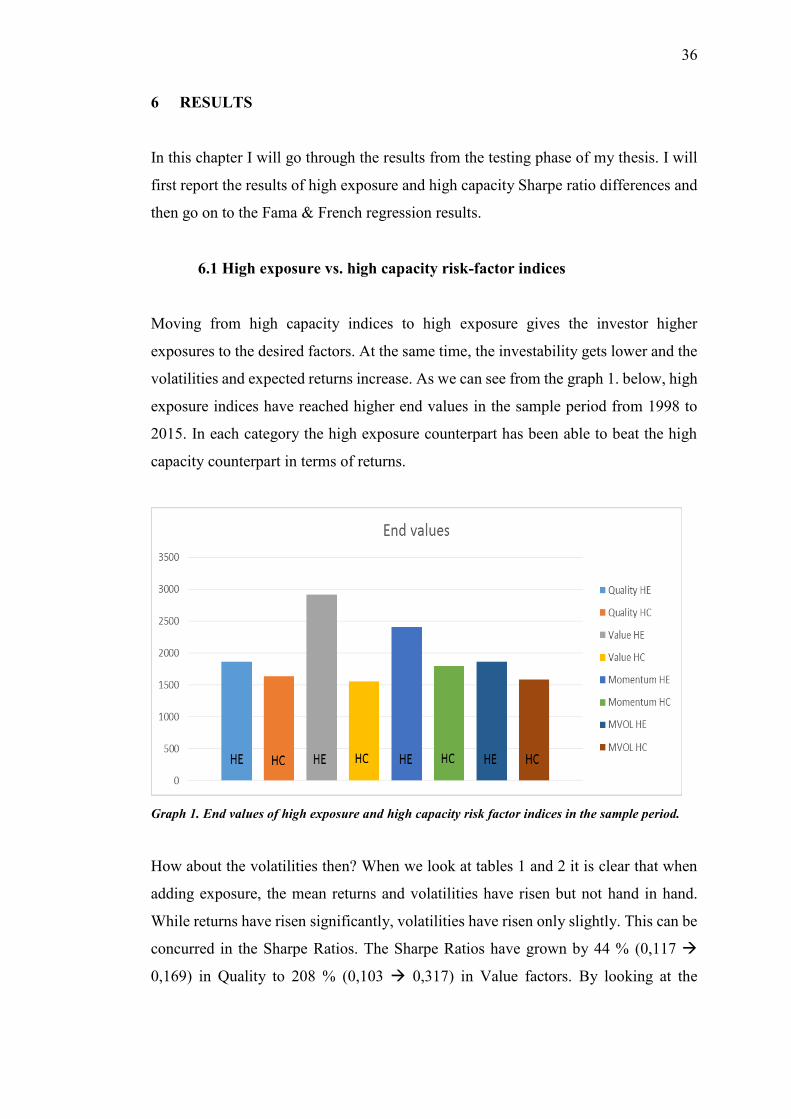
volatilities and expected returns increase. As we can see from the graph 1. below, high
exposure indices have reached higher end values in the sample period from 1998 to
2015. In each category the high exposure counterpart has been able to beat the high
capacity counterpart in terms of returns.
Graph 1. End values of high exposure and high capacity risk factor indices in the sample period.
How about the volatilities then? When we look at tables 1 and 2 it is clear that when
adding exposure, the mean returns and volatilities have risen but not hand in hand.
While returns have risen significantly, volatilities have risen only slightly. This can be
concurred in the Sharpe Ratios. The Sharpe Ratios have grown by 44 % (0,117
0,169) in Quality to 208 % (0,103 0,317) in Value factors. By looking at the
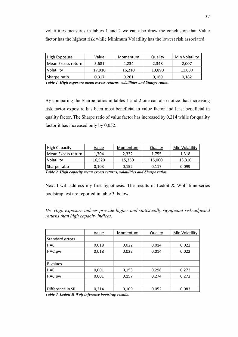
37
volatilities measures in tables 1 and 2 we can also draw the conclusion that Value
factor has the highest risk while Minimum Volatility has the lowest risk associated.
High Exposure Value Momentum Quality Min Volatility
Mean Excess return 5,681 4,234 2,348 2,007
Volatility 17,910 16,210 13,890 11,030
Sharpe ratio 0,317 0,261 0,169 0,182 Table 1. High exposure mean excess returns, volatilities and Sharpe ratios.
By comparing the Sharpe ratios in tables 1 and 2 one can also notice that increasing
risk factor exposure has been most beneficial in value factor and least beneficial in
quality factor. The Sharpe ratio of value factor has increased by 0,214 while for quality
factor it has increased only by 0,052.
High Capacity Value Momentum Quality Min Volatility
Mean Excess return 1,704 2,332 1,755 1,318
Volatility 16,520 15,350 15,000 13,310
Sharpe ratio 0,103 0,152 0,117 0,099 Table 2. High capacity mean excess returns, volatilities and Sharpe ratios.
Next I will address my first hypothesis. The results of Ledoit & Wolf time-series
bootstrap test are reported in table 3. below.
H0: High exposure indices provide higher and statistically significant risk-adjusted
returns than high capacity indices.
Value Momentum Quality Min Volatility
Standard errors
HAC 0,018 0,022 0,014 0,022
HAC.pw 0,018 0,022 0,014 0,022
P-values
HAC 0,001 0,153 0,298 0,272
HAC.pw 0,001 0,157 0,274 0,272
Difference in SR 0,214 0,109 0,052 0,083 Table 3. Ledoit & Wolf inference bootstrap results.

38
To interpret the Ledoit-Wolf results it is important to revise their testing methods.
Their null-hypothesis is that the two Sharpe ratios are equal. This can be rephrased so
that the difference of Sharpe ratios is equal to zero. We can reject the null-hypothesis
if the HAC.pw P-value is below 0,05. This indicates that the Sharpe ratios of high
exposure and high capacity indices are different only for the value factor. It seems that
MSCI risk factor indices can’t produce statistically significant and higher risk-adjusted
returns by increasing the exposure of the risk factor. The value factor seems to be an
exception to the rule. So we can reject the null hypothesis for momentum, quality and
minimum volatility indices. However, for value factor we can’t reject the null
hypothesis and we conclude that higher exposure to value factor provides higher and
statistically significant risk-adjusted returns.
This may be due to the fact that value factor has the highest difference in Sharpe ratios.
The differences for momentum, quality and minimum volatility factors are between
0,052 and 0,109 so it is highly unlikely to get confidence intervals that don’t include
zero. For all risk factor indices it is beneficial to gain higher exposure but we can’t
conclude that it is statistically so.
6.2 Fama & French regressions
For the Fama & French regressions, I have divided the testing in three stages. In the
first phase I will test MSCI’s individual risk factor indices with the Fama & French
factor model with the addition of Carhart Momentum factor. Then I will test how much
the MSCI World index returns can explain the individual risk factor indices returns.
This way I will find out how much the MSCI risk factor indices provide exposure to
the four academic factors and how much have they been tilted away from the parent
index. In the third phase I have constructed different portfolios from the risk factor
indices by utilizing risk parity methods. I will test whether it is possible to beat the
MSCI Diversified Factor Mix index that has equal weights in all the six risk factor
indices. I will also test how well the Fama, French & Carhart model can explain the
returns of these portfolios. Next I will address my second hypothesis shown below.
H0: MSCI factor indices provide statistically significant excess returns.
39
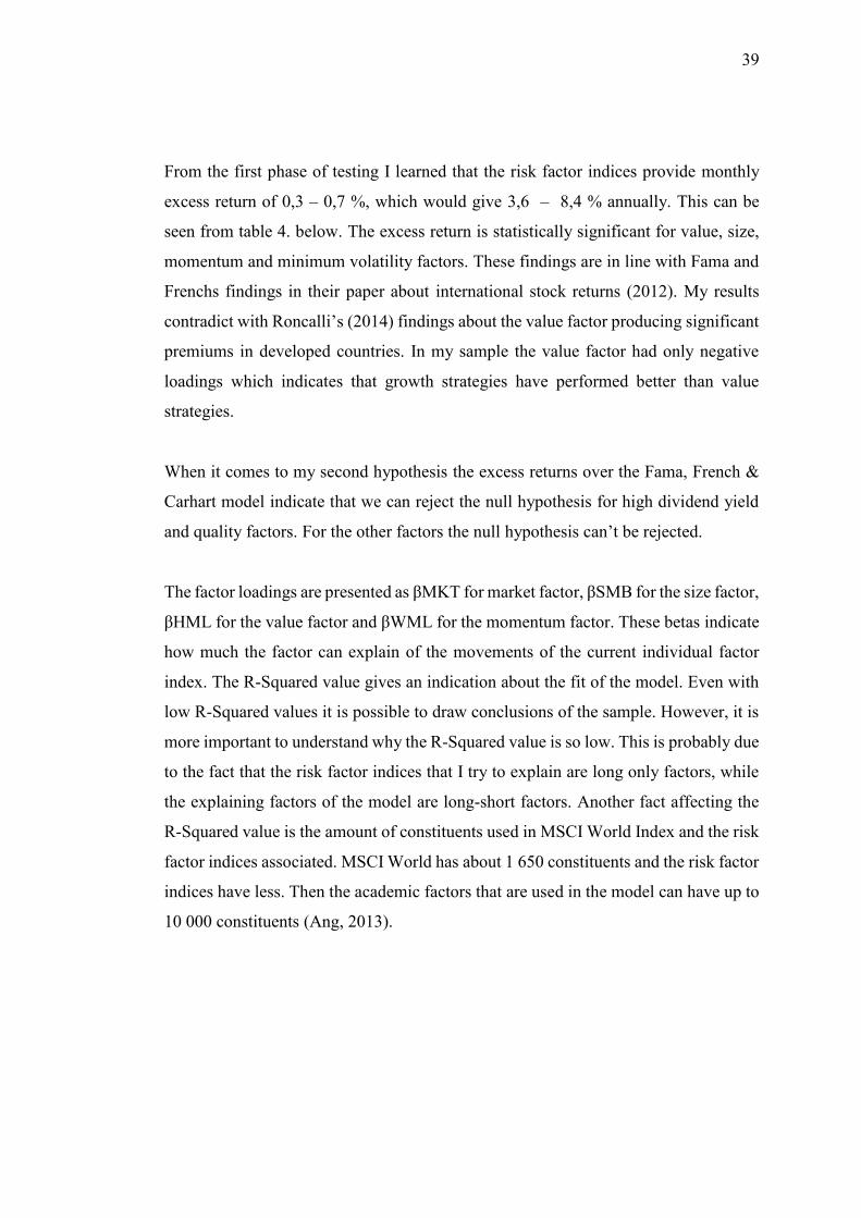
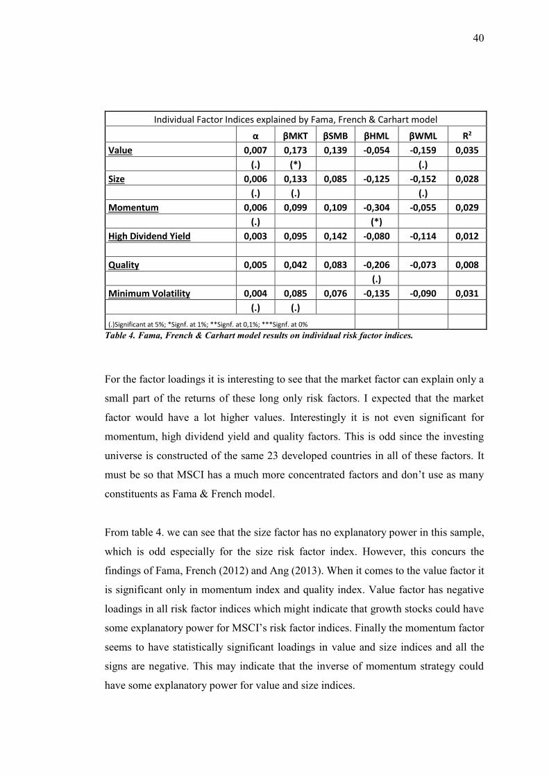
From the first phase of testing I learned that the risk factor indices provide monthly
excess return of 0,3 – 0,7 %, which would give 3,6 – 8,4 % annually. This can be
seen from table 4. below. The excess return is statistically significant for value, size,
momentum and minimum volatility factors. These findings are in line with Fama and
Frenchs findings in their paper about international stock returns (2012). My results
contradict with Roncalli’s (2014) findings about the value factor producing significant
premiums in developed countries. In my sample the value factor had only negative
loadings which indicates that growth strategies have performed better than value
strategies.
When it comes to my second hypothesis the excess returns over the Fama, French &
Carhart model indicate that we can reject the null hypothesis for high dividend yield
and quality factors. For the other factors the null hypothesis can’t be rejected.
The factor loadings are presented as βMKT for market factor, βSMB for the size factor,
βHML for the value factor and βWML for the momentum factor. These betas indicate
how much the factor can explain of the movements of the current individual factor
index. The R-Squared value gives an indication about the fit of the model. Even with
low R-Squared values it is possible to draw conclusions of the sample. However, it is
more important to understand why the R-Squared value is so low. This is probably due
to the fact that the risk factor indices that I try to explain are long only factors, while
the explaining factors of the model are long-short factors. Another fact affecting the
R-Squared value is the amount of constituents used in MSCI World Index and the risk
factor indices associated. MSCI World has about 1 650 constituents and the risk factor
indices have less. Then the academic factors that are used in the model can have up to
10 000 constituents (Ang, 2013).
40
Table 4. Fama, French & Carhart model results on individual risk factor indices.
For the factor loadings it is interesting to see that the market factor can explain only a
small part of the returns of these long only risk factors. I expected that the market
factor would have a lot higher values. Interestingly it is not even significant for
momentum, high dividend yield and quality factors. This is odd since the investing
universe is constructed of the same 23 developed countries in all of these factors. It
must be so that MSCI has a much more concentrated factors and don’t use as many
constituents as Fama & French model.
From table 4. we can see that the size factor has no explanatory power in this sample,
which is odd especially for the size risk factor index. However, this concurs the
findings of Fama, French (2012) and Ang (2013). When it comes to the value factor it
is significant only in momentum index and quality index. Value factor has negative
loadings in all risk factor indices which might indicate that growth stocks could have
some explanatory power for MSCI’s risk factor indices. Finally the momentum factor
seems to have statistically significant loadings in value and size indices and all the
signs are negative. This may indicate that the inverse of momentum strategy could
have some explanatory power for value and size indices.
Individual Factor Indices explained by Fama, French & Carhart model
α βMKT βSMB βHML βWML R2
Value 0,007 0,173 0,139 -0,054 -0,159 0,035
(.) (*) (.)
Size 0,006 0,133 0,085 -0,125 -0,152 0,028
(.) (.) (.)
Momentum 0,006 0,099 0,109 -0,304 -0,055 0,029
(.) (*)
High Dividend Yield 0,003 0,095 0,142 -0,080 -0,114 0,012
Quality 0,005 0,042 0,083 -0,206 -0,073 0,008
(.)
Minimum Volatility 0,004 0,085 0,076 -0,135 -0,090 0,031
(.) (.)
(.)Significant at 5%; *Signf. at 1%; **Signf. at 0,1%; ***Signf. at 0%
41
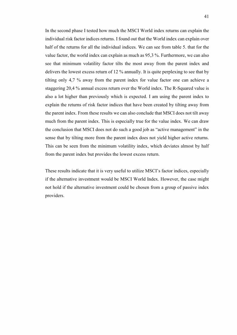
In the second phase I tested how much the MSCI World index returns can explain the
individual risk factor indices returns. I found out that the World index can explain over
half of the returns for all the individual indices. We can see from table 5. that for the
value factor, the world index can explain as much as 95,3 %. Furthermore, we can also
see that minimum volatility factor tilts the most away from the parent index and
delivers the lowest excess return of 12 % annually. It is quite perplexing to see that by
tilting only 4,7 % away from the parent index for value factor one can achieve a
staggering 20,4 % annual excess return over the World index. The R-Squared value is
also a lot higher than previously which is expected. I am using the parent index to
explain the returns of risk factor indices that have been created by tilting away from
the parent index. From these results we can also conclude that MSCI does not tilt away
much from the parent index. This is especially true for the value index. We can draw
the conclusion that MSCI does not do such a good job as “active management” in the
sense that by tilting more from the parent index does not yield higher active returns.
This can be seen from the minimum volatility index, which deviates almost by half
from the parent index but provides the lowest excess return.
These results indicate that it is very useful to utilize MSCI’s factor indices, especially
if the alternative investment would be MSCI World Index. However, the case might
not hold if the alternative investment could be chosen from a group of passive index
providers.
42
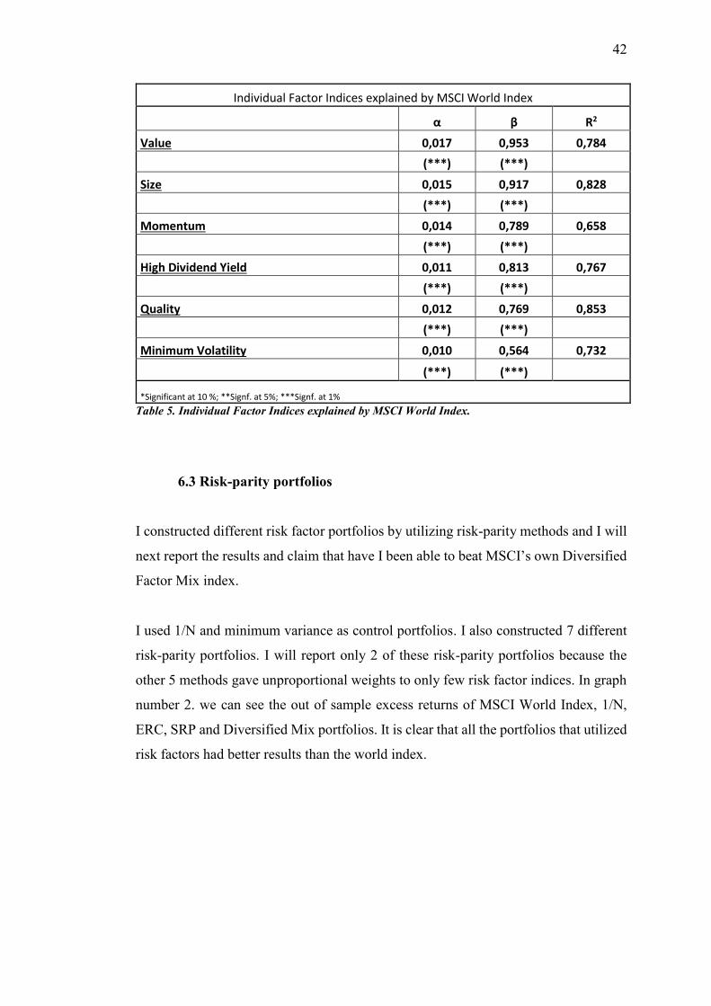
Individual Factor Indices explained by MSCI World Index
α β R2
Value 0,017 0,953 0,784
(***) (***)
Size 0,015 0,917 0,828
(***) (***)
Momentum 0,014 0,789 0,658
(***) (***)
High Dividend Yield 0,011 0,813 0,767
(***) (***)
Quality 0,012 0,769 0,853
(***) (***)
Minimum Volatility 0,010 0,564 0,732
(***) (***)
*Significant at 10 %; **Signf. at 5%; ***Signf. at 1%
Table 5. Individual Factor Indices explained by MSCI World Index.
6.3 Risk-parity portfolios
I constructed different risk factor portfolios by utilizing risk-parity methods and I will
next report the results and claim that have I been able to beat MSCI’s own Diversified
Factor Mix index.
I used 1/N and minimum variance as control portfolios. I also constructed 7 different
risk-parity portfolios. I will report only 2 of these risk-parity portfolios because the
other 5 methods gave unproportional weights to only few risk factor indices. In graph
number 2. we can see the out of sample excess returns of MSCI World Index, 1/N,
ERC, SRP and Diversified Mix portfolios. It is clear that all the portfolios that utilized
risk factors had better results than the world index.
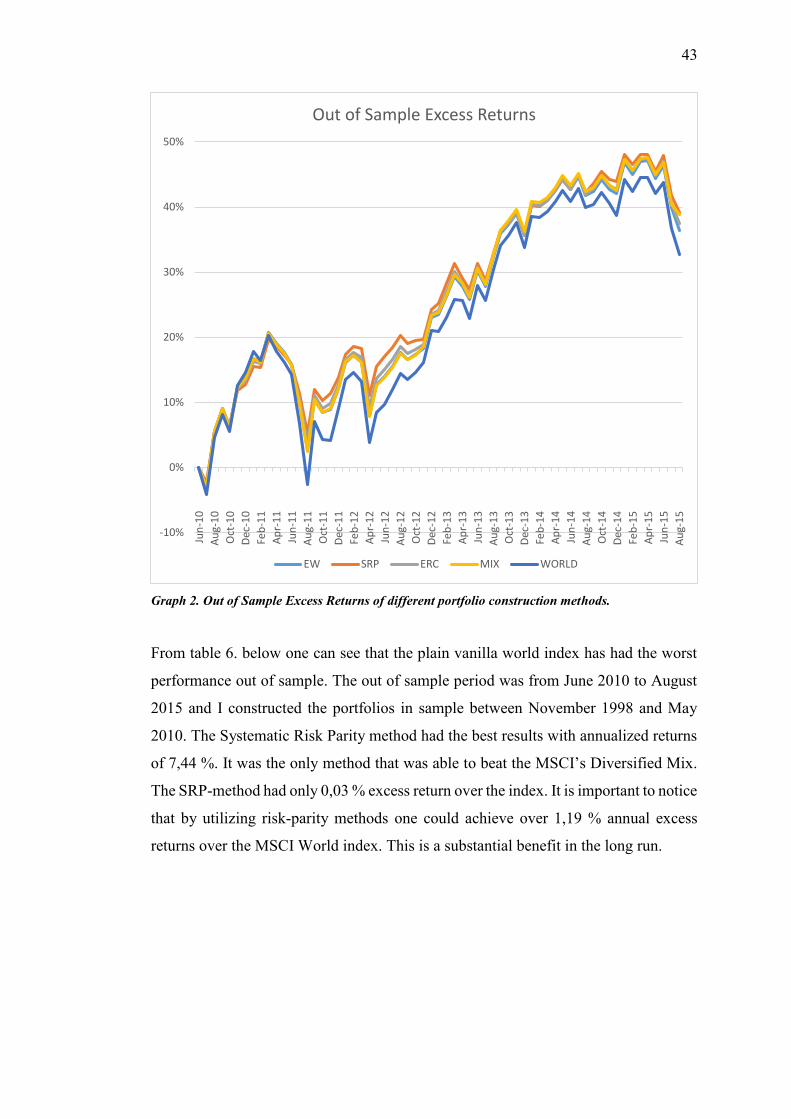
43
Graph 2. Out of Sample Excess Returns of different portfolio construction methods.
From table 6. below one can see that the plain vanilla world index has had the worst
performance out of sample. The out of sample period was from June 2010 to August
2015 and I constructed the portfolios in sample between November 1998 and May
2010. The Systematic Risk Parity method had the best results with annualized returns
of 7,44 %. It was the only method that was able to beat the MSCI’s Diversified Mix.
The SRP-method had only 0,03 % excess return over the index. It is important to notice
that by utilizing risk-parity methods one could achieve over 1,19 % annual excess
returns over the MSCI World index. This is a substantial benefit in the long run.
-10%
0%
10%
20%
30%
40%
50%
Jun
-10
Au
g-1
0
Oct
-10
Dec
-10
Feb
-11
Ap
r-1
1
Jun
-11
Au
g-1
1
Oct
-11
Dec
-11
Feb
-12
Ap
r-1
2
Jun
-12
Au
g-1
2
Oct
-12
Dec
-12
Feb
-13
Ap
r-1
3
Jun
-13
Au
g-1
3
Oct
-13
Dec
-13
Feb
-14
Ap
r-1
4
Jun
-14
Au
g-1
4
Oct
-14
Dec
-14
Feb
-15
Ap
r-1
5
Jun
-15
Au
g-1
5
Out of Sample Excess Returns
EW SRP ERC MIX WORLD
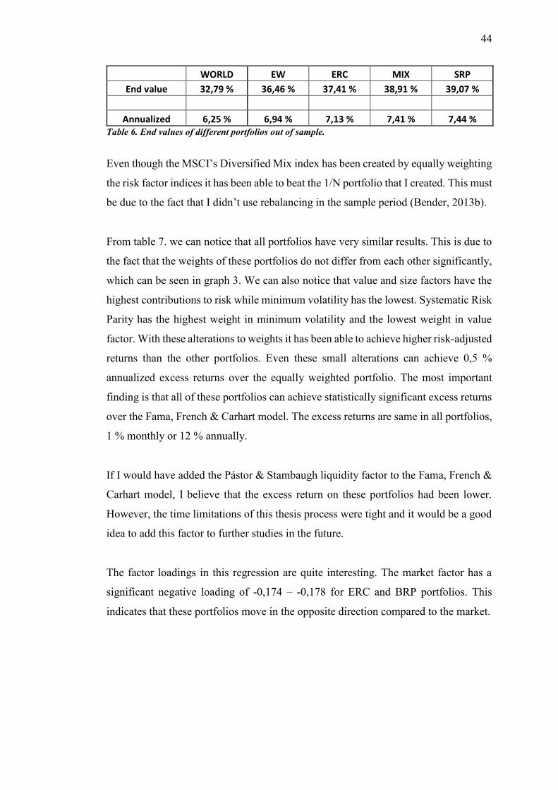
44
WORLD EW ERC MIX SRP
End value 32,79 % 36,46 % 37,41 % 38,91 % 39,07 %
Annualized 6,25 % 6,94 % 7,13 % 7,41 % 7,44 % Table 6. End values of different portfolios out of sample.
Even though the MSCI’s Diversified Mix index has been created by equally weighting
the risk factor indices it has been able to beat the 1/N portfolio that I created. This must
be due to the fact that I didn’t use rebalancing in the sample period (Bender, 2013b).
From table 7. we can notice that all portfolios have very similar results. This is due to
the fact that the weights of these portfolios do not differ from each other significantly,
which can be seen in graph 3. We can also notice that value and size factors have the
highest contributions to risk while minimum volatility has the lowest. Systematic Risk
Parity has the highest weight in minimum volatility and the lowest weight in value
factor. With these alterations to weights it has been able to achieve higher risk-adjusted
returns than the other portfolios. Even these small alterations can achieve 0,5 %
annualized excess returns over the equally weighted portfolio. The most important
finding is that all of these portfolios can achieve statistically significant excess returns
over the Fama, French & Carhart model. The excess returns are same in all portfolios,
1 % monthly or 12 % annually.
If I would have added the Pástor & Stambaugh liquidity factor to the Fama, French &
Carhart model, I believe that the excess return on these portfolios had been lower.
However, the time limitations of this thesis process were tight and it would be a good
idea to add this factor to further studies in the future.
The factor loadings in this regression are quite interesting. The market factor has a
significant negative loading of -0,174 – -0,178 for ERC and BRP portfolios. This
indicates that these portfolios move in the opposite direction compared to the market.

45
Graph 3. Marginal Risk Contributions and Weights of test portfolios.
The size factor seems to have the highest explanatory power and it can explain over
50 % of the returns of my portfolios. All the loadings are statistically significant and
which indicates that the size factor is the main driver behind these returns. These
findings contradict Fama & French (2012) findings about international stock returns.
Value and momentum factors did not get significant loadings and so no conclusions
can be drawn from them.
Risk Factor portfolios explained by Fama, French & Carhart model
α βMKT βSMB βHML βWML R2
EW 0,010 -0,181 0,579 0,348 -0,058 0,050
(.) (*)
ERC 0,010 -0,178 0,564 0,324 -0,060 0,051
(.) (.) (*)
BRP 0,010 -0,174 0,537 0,281 -0,063 0,053
(*) (.) (.)
(.)Significant at 5%; *Signf. at 1%; **Signf. at 0,1%; ***Signf. at 0%
Table 7. Risk parity portfolios explained by Fama, French & Carhart model.
If you compare the regression results of individual indices and risk factor portfolios
constructed from the individual indices, you might notice that the market beta and
value beta have changed their signs. This is simply because the sample is of different
0
0,05
0,1
0,15
0,2
0,25
0,3
0,35
Value Size Mom HDY Qual Minvol
Marginal Risk Contributions & Weights
EW MRC ERC MRC SRP MRC EW ERC SRP

46
length. The individual indices are tested over a period of 1998 to 2015 when the risk
factor portfolios are tested out of sample over 2009 to 2015. This is the primary reason
for differences in results between tables 4. and 7.
These results concur that risk factor investing can be profitable. I was able to beat the
MSCI’s Diversified Mix index and anyone could beat the MSCI World Index by
investing in MSCI’s own risk factor indices. These risk factor indices are widely
available and for example Blackrock already provides ETF’s that track these risk factor
indices.
47
7 CONCLUSION
The purpose of this thesis was to test academically how well MSCI constructs their
risk factor indices. I tested whether MSCI is able to provide higher risk-adjusted
returns by adding risk factor exposure. Then I also tested academically how well can
the Fama & French three factor-model with the addition of Carhart momentum factor
explain the returns of MSCI’s risk factor indices. Finally I tested whether it was
possible to beat MSCI’s own Diversified Mix index that invests in all six risk factors.
I constructed different portfolios with risk-parity methods and tested their performance
against the Diversified Mix index. The main conclusions of this study are opened
below.
High exposure indices had higher returns than their high capacity counterparts in the
sample period. Volatilities also increased when proceeding to high exposure indices
but not as much as expected. The Sharpe ratios of high exposure indices were higher
for all four counterparts but after testing the difference with Ledoit & Wolf inference
method, we could conclude that only value factor had statistically significant and
higher risk-adjusted returns than its high capacity counterpart. So we can reject the
null hypothesis for momentum, quality and minimum volatility indices but not for
value index. I also found out that from these four risk factors, value is the riskiest factor
and minimum volatility has the lowest risk associated.
In the time-series regression tests, I found out that all the individual risk factor indices
provide excess returns over the Fama, French & Carhart model. The excess returns are
statistically significant for value, size, momentum and minimum volatility indices. So
we can conclude that the null hypothesis holds true for value, size, momentum and
minimum volatility but we can reject it for high dividend yield and quality indices. An
interesting finding about the betas in this test was that the market factor does not have
statistically significant explanatory power for momentum, high dividend yield and
quality factors. I expected that the market factor would have high explanatory powers
because it is the only factor that is long only like the MSCI’s risk factor indices.
I also found out that MSCI does not tilt away from the parent index that much. For the
value risk factor index, the parent index MSCI World can explain 95,3 % of the returns.
48
However, for minimum volatility the explanatory power is only 56,4 %. This is partly
due to the fact that minimum volatility has higher concentrations in low volatility
stocks and has higher active risk compared to value index. For the other four factor
indices, the MSCI World can explain over three quarters of the returns. This thesis has
provided new information about the explanatory power of the parent index in MSCI’s
risk factor indices. This is meaningful information when comparing index providers.
High betas indicate low deviation from the parent index which can be seen negatively,
when the idea of building different indices is to create something different from the
parent index.
The individual index tests supported the finding by Ang (2013) that the size factor has
disappeared. However, these results are overruled by the risk-parity portfolio tests
where the size factor was the only factor that had significant positive loadings. The
findings of Roncalli (2014) about the value factor were also contradicted in my results.
Fama & French (2012) paper about international stock returns had a lot of similarities
with my thesis. Their findings about size factor was concurred in my results. They
found significant premiums for the value factor while I found none.
Even with the low R-Squared values one can generalize the results to two key points:
Risk factor investing is able to provide excess returns over MSCI’s World index and
risk-parity methods are able to provide excess returns over equally weighted risk factor
indices.
The testing has been done with robust estimators and the sample size is large enough.
It is also important to notice that the data has been collected with high precision. The
investment universe for all indices and factors is the same 23 developed countries, they
are all quoted in USD and the risk free rate is also quoted in USD. The restrictions that
I utilized in the portfolio construction phase regarding shorting and leverage are
common in industry research. It is important to test these phenomena so that normal
investors can also gain access to the investment portfolios. Because of these
restrictions anyone who reads this thesis could beat the MSCI World Index by
investing in MSCI’s risk factor indices with equal weights.

49
I gained a broad understanding about factor investing through this thesis process and
I found ideas for further research behind every corner. It would be very easy to conduct
a similar study with different data gathered from other index providers like Russell or
FTSE. Even more valuable study would be to go to the constituent level and try to beat
the index providers with the researchers own portfolio construction methods.
50
REFERENCES
Ang, A. (2013). Factor Investing. SSRN Columbia Business School Research
Paper No. 13-42. Available at: <http://ssrn.com/abstract=2277397>. Cited
21.9.2015.
Banz, R. W. (1981). The Relationship Between Return and Market Value of
Common Stocks. Journal of Financial Economics 9: 3-18.
Bender, J., Briand, R., Melas, D. & Subramanian, R. A. (2013a). Foundations of
Factor Investing. MSCI Research Insight. Available at:
<https://www.msci.com/resources/pdfs/Foundations_of_Factor_Investing.pdf>.
Cited 18.10.2015.
Bender, J., Briand, R., Melas, D., Subramanian, R. A. & Subramanian, M.
(2013b). Deploying Multi-Factor Index Allocations in Institutional Portfolios.
MSCI Research Insight. Available at:
<https://www.msci.com/resources/pdfs/Deploying_Multi_Factor_Index_Allocatio
ns_in_Institutional_Portfolios.pdf>. Cited 24.11.2015.
Bruder, B. & Roncalli, T. (2012). Managing Risk Exposures Using the Risk
Budgeting Approach. Available at: <http://ssrn.com/abstract=2009778> Cited
01.10.2015.
Carhart, M. (1997). On Persistence in Mutual Fund Performance. The Journal of
Finance 52(1): 57-82.
Cochrane, J. (1999). New Facts in Finance. Economic Perspectives Federal
Reserve Bank of Chigaco 23(3): 36-58.
Cochrane, J. (2007). Efficient markets today. Conference on Chicago Economics.
Available at: <http://faculty-chicago.edu/john.cochrane/>. Cited 25.09.2015.
Cochrane, J. (2011). Presidential address: Discount rates. The Journal of Finance
LXVI (4): 1047-1108.
51
Fama, E. & French, K. (1992). The Cross-Section of Expected Stock Returns.
Journal of Financial Economics 22: 3-25.
Fama, E. & French, K. (1993). Common Risk Factors in the Returns on Stocks
and Bonds. Journal of Financial Economics 33: 3-56.
Fama, E. & French, K. (1996). Multifactor Explanations of Asset Pricing
Anomalies. Journal of Finance 51(1): 55-84.
Fama, E. & French, K. (2012). Size, Value, and Momentum in International Stock
Returns. Journal of Financial Economics 105(3): 457-472.
French, K. (2008). The Cost of Active Investing. SSRN Darthmouth College –
Tuck School of Business. Available at: < http://ssrn.com/abstract=1105775>.
Cited 28.09.2015.
Grossman, S. & Stiglitz, J. (1980) On the Impossibility of Informationally
Efficient Markets. The American Economic Review 70(3): 393-408.
Israel, R. & Moskowitz, T. (2012). The Role of Shorting, Firm Size, and Time on
Market Anomalies. SSRN University of Chigaco Booth Research Paper No. 12-
22. Available at: < http://ssrn.com/abstract=2089466>. Cited 21.9.2015.
Jagadeesh, N. and Titman, S. (1993). Returns to Buying Winners and Selling
Losers: Implications for Market Efficiency. Journal of Finance 48(1): 65–91.
Kahra, H. (2015). Katsaus institutionaalisen sijoittamisen periaatteisiin ja
menetelmiin. Eläketurvakeskuksen raportteja 01/2015.
Ledoit, O. & Wolf, M. (2008). Robust performance hypothesis testing with the
Sharpe ratio. Journal of Empirical Finance 15: 850-859.
Lintner, J. (1965). The Valuation of Risk Assets and the Selection of Risky
Investments in Stock Portfolios and Capital Budgets. The Review of Economics
and Statistics 47(1): 13-37.
52
Maillard, S., Roncalli, T. & Teïlechte, J. (2010). The Properties of Equally
Weighted Risk Contribution Portfolios. The Journal of Portfolio Management
36(4): 60-70.
Malkiel, B. (2003). Passive Investment Strategies and Efficient Markets.
European Financial Management 9(1): 1-10.
Markowitz, H. (1952). Portfolio selection. Journal of Finance 7(1): 77-91.
Mossin, J. (1966), Equilibrium in a Capital Asset Market. The Econometric
Society 34(4): 768-783.
Pástor, L. & Stambaugh, R. (2013), Liquidity Risk and Expected Stock Returns.
Journal of Political Economy 111(3): 642-685.
Roncalli, T. (2014), Risk Factor Investing Explained. Investment Insights form
Lyxor Asset Management 1-4. Available at:
<https://www.fondsnieuws.nl/system/storage/serve/117876/Expert_opinion_lyxor
.pdf.> Cited 04.12.2015.
Rosenberg, B., Reid, K. & Lanstein, R. (1985). Persuasive Evidence of Market
Inefficiency. Journal of Porfolio Management 11: 9-16.
Ross, S. (1976). The Arbitrage Theory of Capital Asset Pricing. Journal of
Economic Theory 13: 341-360.
Rubinstein, M. (2006). A History of the Theory of Investments: My Annotated
Bibliography. John Wiley & Sons.
Sharpe, W. (1964). A theory of Market Equilibrium under Conditions of Risk.
The Journal of Finance 19(3): 425-442.
Sharpe, W. (1991). The Arithmetic of Active Management. Financial Analysts
Journal 47(1): 7-9.

53
Shores, S. (2015). Smart Beta: Defining the Opportunity and Solutions. Blackrock
Industry Research. Available at: <https://www.blackrock.com/institutions/en-
us/literature/whitepaper/smart-beta-defining-the-opportunity-and-solutions.pdf>.
Cited 26.11.2015.
Treynor, J. L. (1961). Market Value, Time, And Risk. Unpublished manuscript.
Rough Draft dated 8/8/61: 95-209.

54
TABLES AND FIGURES
Picture 1. presents the unavoidable trade-off between investability and risk factor
exposure.
Picture 2. presents the dimensions of investability.
Graph 1. presents the end values of high exposure and high capacity risk factor indices
in the sample period.
Graph 2. presents the out of sample excess returns of different portfolio construction
methods.
Graph 3. presents the marginal risk contributions and weights of test portfolios.
Table 1. presents the high exposure mean excess returns, volatilities and Sharpe ratios
Table 2. presents the high capacity mean excess returns, volatilities and Sharpe ratios.
Table 3. presents the Ledoit & Wolf inference bootstrap results
Table 4. presents the Fama, French & Carhart model results on individual risk factor
indices.
Table 5. presents the individual factor indices explained by MSCI World Index.
Table 6. presents the end values of different portfolios out of sample.
Table 7. presents the Risk-parity portfolios explained by Fama, French & Carhart
model.