jpm credit derivatives
TRANSCRIPT

5/10/2018 JPM Credit Derivatives - slidepdf.com
http://slidepdf.com/reader/full/jpm-credit-derivatives-559e0102dc371 1/180
The certifying analyst(s) is indicated by a superscript AC. See last page of thereport for analyst certification and important legal and regulatory disclosures.
www.morganmarkets.com
About this handbook
This handbook reviews both the basic concepts and more advancedtrading strategies made possible by the credit derivatives market. Readersseeking an overview should consider Sections 1.1 - 1.3, and 8.1.
There are four parts to this handbook:
Part I: Credit default swap fundamentals 5
Part I introduces the CDS market, its participants, and the mechanics of the credit default swap. This section provides intuition about the CDSvaluation theory and reviews how CDS is valued in practice. Nuances of the standard ISDA documentation are discussed, as are developments indocumentation to facilitate settlement following credit events.
Part II: Valuation and trading strategies 43
Part II provides a comparison of bonds and credit default swaps and
discusses why CDS to bond basis exists. The theory behind CDS curvetrading is analyzed, and equal-notional, duration-weighted, and carry-neutral trading strategies are reviewed. Credit versus equity tradingstrategies, including stock and CDS, and equity derivatives and CDS, areanalyzed.
Part III: Index products 111
The CDX and iTraxx products are introduced, valued and analyzed.Options on these products are explained, as well as trading strategies.Tranche products, including CDOs, CDX and iTraxx tranches, Tranchlets,options on Tranches, and Zero Coupon equity are reviewed.
Part IV: Other CDS products 149
Part IV covers loan CDS, preferred CDS, Recovery Locks, Digital defaultswaps, credit-linked notes, constant maturity CDS, and first to default baskets.
JPMorgan publishes daily reports that analyze the credit derivativemarkets. To receive electronic copies of these reports, please contact a
Credit Derivatives research professional or your salesperson. Thesereports are also available on www.morganmarkets.com.
Corporate Quantitative ResearchNew York, LondonDecember, 2006
Credit Derivatives HandbookDetailing credit default swap products, markets and
trading strategies
Corporate Quantitative Research
Eric BeinsteinAC
(1-212) [email protected]
Andrew Scott, CFA (1-212) 834-3843
Ben Graves, CFA (1-212) 622-4195
Alex Sbityakov (1-212) 834-3896
Katy Le (1-212) 834-4276
European Credit Derivatives Research
Jonny Goulden (44-20) 7325-9582
Dirk Muench (44-20) 7325-5966
Saul Doctor (44-20) 7325-3699
Andrew Granger (44-20) 7777-1025
Yasemin Saltuk (44-20) 7777-1261
Peter S Allen (44-20) 7325-4114

5/10/2018 JPM Credit Derivatives - slidepdf.com
http://slidepdf.com/reader/full/jpm-credit-derivatives-559e0102dc371 2/180
Eric Beinstein (1-212) [email protected]
Andrew Scott, CFA (1-212) [email protected]
Corporate Quantitative ResearchCredit Derivatives HandbookDecember, 2006
2
Part I: Credit default swap fundamentals ........................................................................................................5
1. Introduction..........................................................................................................................................................................6
2. The credit default swap .......................................................................................................................................................8 Credit events........................................................................................................................................................................9 Settlement following credit events ....................................................................................................................................10 Monetizing CDS contracts.................................................................................................................................................11 Counterparty considerations..............................................................................................................................................12 Accounting for CDS..........................................................................................................................................................12
3. Marking CDS to market: CDSW .....................................................................................................................................13
4. Valuation theory and credit curves ..................................................................................................................................15 Default probabilities and CDS pricing...............................................................................................................................15 The Shape of Credit Curves...............................................................................................................................................18
Forwards in credit..............................................................................................................................................................20 Summary............................................................................................................................................................................22 Risky Annuities and Risky Durations (DV01) ..................................................................................................................23
5. The ISDA Agreement ........................................................................................................................................................24 Standardized documentation..............................................................................................................................................24 The new CDS settlement protocol.....................................................................................................................................24 CDX Note settlement procedures......................................................................................................................................32 “Old-fashioned” CDS settlement procedures ....................................................................................................................33 Succession events ..............................................................................................................................................................34
6. The importance of credit derivatives................................................................................................................................38
7. Market participants...........................................................................................................................................................40
Part II: Valuation and trading strategies........................................................................................................43 Decomposing risk in a bond ..............................................................................................................................................44 Par-equivalent credit default swap spread .........................................................................................................................46 Methodology for isolating credit risk in bonds with embedded options............................................................................52
9. Basis Trading......................................................................................................................................................................55 Understanding the difference between bonds and credit default swap spreads .................................................................55 Trading the basis................................................................................................................................................................57
10. Trading Credit Curves ....................................................................................................................................................62 Drivers of P+L in curve trades...........................................................................................................................................62 Curve trading strategies .....................................................................................................................................................70 1. Equal-Notional Strategies: Forwards.............................................................................................................................70 2. Duration-weighted strategies.........................................................................................................................................76 3. Carry-neutral strategies..................................................................................................................................................80 Different ways of calculating slide ....................................................................................................................................82 Calculating breakevens......................................................................................................................................................84 The Horizon Effect ............................................................................................................................................................86 Changing Risky Annuities over the Trade Horizon...........................................................................................................86 A worked example.............................................................................................................................................................86 Horizon Effect Conclusion................................................................................................................................................89

5/10/2018 JPM Credit Derivatives - slidepdf.com
http://slidepdf.com/reader/full/jpm-credit-derivatives-559e0102dc371 3/180
Eric Beinstein (1-212) [email protected]
Andrew Scott, CFA (1-212) [email protected]
Corporate Quantitative ResearchCredit Derivatives HandbookDecember, 2006
3
11. Recovery rate and curve shape impact on CDS valuation ...........................................................................................90 Intuition .............................................................................................................................................................................90 CDS curve shape impact....................................................................................................................................................91 Recovery rate impact .........................................................................................................................................................92
Assumptions at contract inception.....................................................................................................................................93 Worked examples ..............................................................................................................................................................94
12. Trading credit versus equity ...........................................................................................................................................97 Relationships in equity and credit markets ........................................................................................................................97 Finding trade ideas.............................................................................................................................................................98 A worked trade recommendation.....................................................................................................................................100
13. Trading CDS against equity puts..................................................................................................................................106
Part III: Index products ..........................................................................................................................................111 Introduction .....................................................................................................................................................................112 Mechanics of the CDX and iTraxx indices......................................................................................................................112
Basis to theoretical...........................................................................................................................................................113 Comparing on-the-run and off-the-run basis ...................................................................................................................114 Credit events....................................................................................................................................................................115 CDX and iTraxx indices ..................................................................................................................................................116 History of US CDS Indices..............................................................................................................................................120
15. CDX and iTraxx options................................................................................................................................................121 Product description..........................................................................................................................................................121 Basic option strategy payoff diagrams.............................................................................................................................122 Using options to express a spread view...........................................................................................................................122 Using options to express a volatility view.......................................................................................................................122 Combining spread and volatility views ...........................................................................................................................123
Option trading strategies..................................................................................................................................................124 The practical side to trading options................................................................................................................................125
16. Trading credit volatility ................................................................................................................................................130 Defining volatility............................................................................................................................................................130 Delta-hedging ..................................................................................................................................................................131 The returns from delta-hedging in credit .........................................................................................................................132 Historical analysis............................................................................................................................................................133 Option glossary................................................................................................................................................................134
17. Tranche products...........................................................................................................................................................136 What is a tranche?............................................................................................................................................................136 Why are synthetic tranches traded? .................................................................................................................................139
The mechanics of trading tranche protection...................................................................................................................141 The role of correlation .....................................................................................................................................................142 Pricing tranches ...............................................................................................................................................................143 Other products .................................................................................................................................................................145
Part IV: Other CDS products ..............................................................................................................................149 Overview .........................................................................................................................................................................150 Comparing CDS contracts across asset classes ...............................................................................................................150 Similarities and differences between CDS and LCDS.....................................................................................................151 Participants ......................................................................................................................................................................154 Settlement following a credit event .................................................................................................................................154 Modifications to LSTA transfer documents ....................................................................................................................156

5/10/2018 JPM Credit Derivatives - slidepdf.com
http://slidepdf.com/reader/full/jpm-credit-derivatives-559e0102dc371 4/180
Eric Beinstein (1-212) [email protected]
Andrew Scott, CFA (1-212) [email protected]
Corporate Quantitative ResearchCredit Derivatives HandbookDecember, 2006
4
Rating agency approach to LCDS in structured credit ....................................................................................................156 Spread relationship between loans and LCDS.................................................................................................................157
19. Preferred CDS................................................................................................................................................................158 Overview .........................................................................................................................................................................158 Preferred stock CDS contracts differ from the standard CDS contract............................................................................158 PCDS versus CDS ...........................................................................................................................................................160 Overview of preferred stock issuance and market...........................................................................................................160
20. Profiting from views on recovery rates ........................................................................................................................162 Recovery Rate Lock ........................................................................................................................................................162 Digital Default Swaps......................................................................................................................................................167
21. Other credit default swap products..............................................................................................................................168 Credit linked notes...........................................................................................................................................................168 Constant maturity credit default swaps (CMCDS) and credit spread swaps (CSS).........................................................169 First-to-default baskets ....................................................................................................................................................170
Conclusion ....................................................................................................................................................................171
Appendix I: JPMorgan CDSW Example Calculations Model .........................................................................................172
Appendix II: How to get CDX and iTraxx data ................................................................................................................173

5/10/2018 JPM Credit Derivatives - slidepdf.com
http://slidepdf.com/reader/full/jpm-credit-derivatives-559e0102dc371 5/180
Eric Beinstein (1-212) [email protected]
Andrew Scott, CFA (1-212) [email protected]
Corporate Quantitative ResearchCredit Derivatives HandbookDecember, 2006
5
Part I: Credit default swap fundamentals
1. Introduction............................................................................................................6
2. The credit default swap .........................................................................................8
Credit events .........................................................................................................9Settlement following credit events......................................................................10Monetizing CDS contracts..................................................................................11Counterparty considerations ...............................................................................12Accounting for CDS ...........................................................................................12
3. Marking CDS to market: CDSW .......................................................................13
4. Valuation theory and credit curves ....................................................................15Default probabilities and CDS pricing................................................................15The Shape of Credit Curves................................................................................18
Forwards in credit ...............................................................................................20Summary.............................................................................................................22Risky Annuities and Risky Durations (DV01) ...................................................23
5. The ISDA Agreement ..........................................................................................24Standardized documentation...............................................................................24The new CDS settlement protocol ......................................................................24CDX Note settlement procedures .......................................................................32“Old-fashioned” CDS settlement procedures .....................................................33Succession events ...............................................................................................34
6. The importance of credit derivatives..................................................................38
7. Market participants.............................................................................................40

5/10/2018 JPM Credit Derivatives - slidepdf.com
http://slidepdf.com/reader/full/jpm-credit-derivatives-559e0102dc371 6/180
Eric Beinstein (1-212) [email protected]
Andrew Scott, CFA (1-212) [email protected]
Corporate Quantitative ResearchCredit Derivatives HandbookDecember, 2006
6
1. Introduction
A credit derivative is a financial contract that allows one to take or reduce credit
exposure, generally on bonds or loans of a sovereign or corporate entity. Thecontract is between two parties and does not directly involve the issuer itself. Creditderivatives are primarily used to:
1) express a positive or negative credit view on a single entity or a portfolio of entities, independent of any other exposures to the entity one might have.
2) reduce risk arising from ownership of bonds or loans
Since its introduction in the mid-1990s, the growth of the credit derivative markethas been dramatic:
• The notional amount of credit derivative contracts outstanding in 2006 is
$20.2 trillion, up 302% from 20041. This amount is greater than the facevalue of corporate and sovereign bonds globally.
• The tremendous growth in the credit derivatives market has been driven bythe standardization of documentation, the growth of product applications,and diversification of participants.
• Credit derivatives have become mainstream and are integrated with credittrading and risk management at many firms.
Exhibit 1.1: The notional amount of credit derivatives globally is larger than the global amount of debt outstanding
$0
$5,000
$10,000
$15,000
$20,000
$25,000
$30,000
$35,000
N o t i o n a l O u t s t a n d i n g ( $ B )
1998 1999 2000 2001 2002 2003 2004 2005 2006 2008E
Cash Bonds Credit Derivatives
Sources: British Bankers’ Association Credit Derivatives Report 2006, Bank for International Settlements and ISDA.
Note: Cash bonds through June 2006.
1British Bankers’ Association estimates.

5/10/2018 JPM Credit Derivatives - slidepdf.com
http://slidepdf.com/reader/full/jpm-credit-derivatives-559e0102dc371 7/180
Eric Beinstein (1-212) [email protected]
Andrew Scott, CFA (1-212) [email protected]
Corporate Quantitative ResearchCredit Derivatives HandbookDecember, 2006
7
A driver of the growth in credit derivatives is the ability to use them to express creditviews not as easily done in cash bonds, for example:
• Relative value, or long and short views between credits
• Capital structure views, i.e., senior versus subordinated trading
• Views about the shape of a company’s credit curve
• Macro strategy views, i.e. investment grade versus high yield portfoliotrading using index products
• Views on credit volatility
• Views on the timing and pattern of defaults, or correlation trading
Single name credit default swaps are the most widely used product, accounting for
33% of volume. Index products account for 30% of volume, and structured credit,including tranched index trading and synthetic collateralized debt obligations,account for another 24%. In this handbook, single name CDS is addressed in Part Iand II, and index and structured credit in Part III. Part IV introduces other CDS products.
Exhibit 1.2: Credit derivative volumes by product
Type 2004 2006
Single-name credit default swaps 51.0% 32.9%
Full index trades 9.0% 30.1%
Synthetic CDOs 16.0% 16.3%
Tranched index trades 2.0% 7.6%
Credit linked notes 6.0% 3.1%
Others 16.0% 10.0%
Sources: British Bankers’ Association Credit Derivatives Report 2006

5/10/2018 JPM Credit Derivatives - slidepdf.com
http://slidepdf.com/reader/full/jpm-credit-derivatives-559e0102dc371 8/180
Eric Beinstein (1-212) [email protected]
Andrew Scott, CFA (1-212) [email protected]
Corporate Quantitative ResearchCredit Derivatives HandbookDecember, 2006
8
2. The credit default swap
The credit default swap (CDS) is the cornerstone of the credit derivatives market. A
credit default swap is an agreement between two parties to exchange the credit risk of an issuer (reference entity). The buyer of the credit default swap is said to buy protection. The buyer usually pays a periodic fee and profits if the reference entityhas a credit event, or if the credit worsens while the swap is outstanding. A creditevent includes bankruptcy, failing to pay outstanding debt obligations, or in someCDS contracts, a restructuring of a bond or loan. Buying protection has a similar credit risk position to selling a bond short, or “going short risk.”
The seller of the credit default swap is said to sell protection. The seller collects the periodic fee and profits if the credit of the reference entity remains stable or improveswhile the swap is outstanding. Selling protection has a similar credit risk position toowning a bond or loan, or “going long risk.”
As shown in Exhibit 2.1, Investor B, the buyer of protection, pays Investor S, theseller of protection, a periodic fee (usually on the 20th of March, June, September,and December) for a specified time frame. To calculate this fee on an annualized basis, the two parties multiply the notional amount of the swap, or the dollar amountof risk being exchanged, by the market price of the credit default swap (the market price of a CDS is also called the spread or fixed rate). CDS market prices are quotedin basis points (bp) paid annually, and are a measure of the reference entity’s creditrisk (the higher the spread the greater the credit risk). (Section 3 and 4 discuss howcredit default swaps are valued.)
Exhibit 2.1: Single name credit default swaps
Definition: A credit default swap is an agreement in which one party buys protection against lossesoccurring due to a credit event of a reference entity up to the maturity date of the swap. The protection
buyer pays a periodic fee for this protection up to the maturity date, unless a credit event triggers thecontingent payment. If such trigger happens, the buyer of protection only needs to pay the accrued fee upto the day of the credit event (standard credit default swap), and deliver an obligation of the referencecredit in exchange for the protection payout.
Source: JPMorgan.
-“Short risk”
-Buy default protection
-Buy CDS
-Pay Periodic Payments
Credit Risk Profile of shorting a bond Credit Risk Profile of owning a bond
-“Long risk”
-Sell default protection
-Sell CDS
-Receive Periodic Payments
ContingentPayment upon a
credit event
ReferenceEntity
Investor B
Protection
Buyer
Investor S
Protection
Seller
Periodic Coupons
Risk (Notional)

5/10/2018 JPM Credit Derivatives - slidepdf.com
http://slidepdf.com/reader/full/jpm-credit-derivatives-559e0102dc371 9/180
Eric Beinstein (1-212) [email protected]
Andrew Scott, CFA (1-212) [email protected]
Corporate Quantitative ResearchCredit Derivatives HandbookDecember, 2006
9
Exhibit 2.2: If the Reference Entity has a credit event, the CDS Buyer delivers a bon d or l oanissued by the reference entity to the Seller. The Seller then delivers the Notional value of theCDS contract to the Buyer.
Source: JPMorgan.
Credit events
A credit event triggers a contingent payment on a credit default swap. Credit eventsare defined in the 2003 ISDA Credit Derivatives Definitions and include thefollowing:
1. Bankruptcy: includes insolvency, appointment of administrators/liquidators,and creditor arrangements.
2. Failure to pay: payment failure on one or more obligations after expiration of any applicable grace period; typically subject to a materiality threshold (e.g.,US$1million for North American CDS contracts).
3. Restructuring: refers to a change in the agreement between the reference entityand the holders of an obligation (such agreement was not previously providedfor under the terms of that obligation) due to the deterioration increditworthiness or financial condition to the reference entity with respect to:
• reduction of interest or principal
• postponement of payment of interest or principal
• change of currency (other than to a “Permitted Currency”)
There are 4 parameters that uniquely define a credit default swap
1. Which credit (note: not which bond, but which issuer)
• Credit default swap contracts specify a reference obligation (a
specific bond or loan) which defines the issuing entity through the bond prospectus. Following a credit event, bonds or loans pari passuwith the reference entity bond or loan are deliverable into thecontract. Typically a senior unsecured bond is the reference entity, but bonds at other levels of the capital structure may be referenced.
2. Notional amount
• The amount of credit risk being transferred. Agreed between the buyer and seller of CDS protection.
3. Spread
• The annual payments, quoted in basis points paid annually.Payments are paid quarterly, and accrue on an actual/360 day basis.The spread is also called the fixed rate, coupon, or price.
4. Maturity
• The expiration of the contract, usually on the 20th of March, June,September or December. The five year contract is usually the mostliquid.

5/10/2018 JPM Credit Derivatives - slidepdf.com
http://slidepdf.com/reader/full/jpm-credit-derivatives-559e0102dc371 10/180
Eric Beinstein (1-212) [email protected]
Andrew Scott, CFA (1-212) [email protected]
Corporate Quantitative ResearchCredit Derivatives HandbookDecember, 2006
10
• contractual subordination
Note that there are several versions of the restructuring credit event that are used indifferent markets.
4. Repudiation/moratorium: authorized government authority (or referenceentity) repudiates or imposes moratorium and failure to pay or restructuringoccurs.
5. Obligation acceleration: one or more obligations due and payable as a result of the occurrence of a default or other condition or event described, other than afailure to make any required payment.
For US high grade markets, bankruptcy, failure to pay, and modified restructuringare the standard credit events. Modified Restructuring is a version of theRestructuring credit event where the instruments eligible for delivery are restricted.European CDS contracts generally use Modified Modified Restructuring (MMR),which is similar to Modified Restructuring, except that it allows a slightly larger
range of deliverable obligations in the case of a restructuring event2
. In the US highyield markets, only bankruptcy and failure to pay are standard. Of the above creditevents, bankruptcy does not apply to sovereign reference entities. In addition,repudiation/moratorium and obligation acceleration are generally only used for emerging market reference entities.
Settlement following credit events
Following a credit event, the buyer of protection (short risk) delivers to the seller of protection defaulted bonds and/or loans with a face amount equal to the notionalamount of the credit default swap contract. The seller of protection (long risk) thendelivers the notional amount on the CDS contract in cash to the buyer of protection. Note that the buyer of protection pays the accrued spread from the last coupon payment date up to the day of the credit event, then the coupon payments stop. The
buyer can deliver any bond issued by the reference entity meeting certain criteria thatis pari passu, or of the same level of seniority, as the specific bond referenced in thecontract. Thus the protection buyer has a “cheapest to deliver option,” as she candeliver the lowest dollar price bond to settle the contract. The value of the bonddelivered is called the recovery rate. Note that the recovery rate in CDS terminologyis different from the eventual workout value of the bonds post bankruptcy proceedings. The recovery rate is the price at which bonds or loans ar trading whenCDS contracts are settled. This CDS settlement process is called “physicalsettlement,” as the “physical” bonds are delivered as per the 2003 ISDA CreditDerivative Definitions3. Specifically, there is a three step physical settlement procedure in which:
2For more information, refer to “The 2003 ISDA Credit Derivatives Definitions” by Jonathan
Adams and Thomas Benison, published in June 2003.3
Copies of the 2003 ISDA Credit Derivatives Definitions can be obtained by visiting theInternational Swaps and Derivatives Association website at http://www.isda.org

5/10/2018 JPM Credit Derivatives - slidepdf.com
http://slidepdf.com/reader/full/jpm-credit-derivatives-559e0102dc371 11/180
Eric Beinstein (1-212) [email protected]
Andrew Scott, CFA (1-212) [email protected]
Corporate Quantitative ResearchCredit Derivatives HandbookDecember, 2006
11
At default, Notification of a credit event: The buyer or seller of protection maydeliver a notice of a credit event to the counterparty. This notice may be legallydelivered up to 14 days after the maturity of the contract, which may be years after the credit event.
Default + 30 days, Notice of physical settlement: Once the “Notification of a creditevent” is delivered, the buyer of protection has 30 calendar days to deliver a “Noticeof physical settlement.” In this notice, the buyer of protection must specify which bonds or loans they will deliver.
Default + 33 days, Delivery of bonds: The buyer of protection typically delivers bonds to the seller within three days after the “Notice of physical settlement” issubmitted.
Alternatively, because the CDS contract is a bilateral agreement, the buyer and seller can agree to unwind the trade based on the market price of the defaulted bond, for example $40 per $100. The seller then pays the net amount owed to the protection buyer, or $100 - $40 = $60. This is called “cash settlement.” It is important to notethat the recovery rate ($40 in this example) is not fixed and is determined only after
the credit event.
Currently, and importantly, the market has drafted an addendum to the 2003 ISDAdefinitions that defines an auction process meant to be a fair, logistically convenientmethod of settling CDS contracts following a credit event. This CDS Settlement protocol is discussed in Section 5.
Monetizing CDS contracts
There does not need to be a credit event for credit default swap investors to capturegains or losses, however. Like bonds, credit default swap spreads widen when themarket perceives credit risk has increased and tightens when the market perceivescredit risk has improved. For example, if Investor B bought five years of protection
(short risk) paying 50bp per year, the CDS spread could widen to 75bp after one year.
Investor B could monetize her unrealized profits using two methods. First, she couldenter into the opposite trade, selling four-year protection (long risk) at 75bp. Shecontinues to pay 50bp annually on the first contract, thus nets 25bp per year until thetwo contracts mature, effectively locking in her profits. The risk to Investor B is that if the credit defaults, the 50bp and 75bp payments stop, and she no longer enjoys the25bp difference. Otherwise, she is default neutral since she has no additional gain or loss if a default occurs, in which case she just stops benefiting from the 25bp per year income.
The second, more common method to monetize trades is to unwind them. Investor Bcan unwind the 50bp short risk trade with Investor S or another dealer, presumablyfor a better price. Investor B would receive the present value of the expected future payments. Namely, 75 – 50 = 25bp for the remaining four years on her contract,multiplied by the notional amount of the swap, and multiplied by the probability thatthe credit does not default. After unwinding the trade, investors B has nooutstanding positions. The JPMorgan “CDSW” calculator on Bloomberg is theindustry standard method of calculating unwind prices, and is explained in Section 3.

5/10/2018 JPM Credit Derivatives - slidepdf.com
http://slidepdf.com/reader/full/jpm-credit-derivatives-559e0102dc371 12/180
Eric Beinstein (1-212) [email protected]
Andrew Scott, CFA (1-212) [email protected]
Corporate Quantitative ResearchCredit Derivatives HandbookDecember, 2006
12
Exhibit 2.3: CDS investors can capture gains and losses before a CDS contract matures.
Note: Investor B may directly unwind Trade 1 with Investor S, or instead with Investor B2 (presumablyfor a better price). If she chooses to do the unwind trade with Investor B2, she tells Investor B2 that she isassigning her original trade with S to Investor B2. Investor S and Investor B2 then have offsetting tradeswith each other. In either case her profit is the same. She would receive the present value of (75 - 50 = 25
bp) * (4, approximate duration of contract) * (notional amount of the swap). Thus, Investor B finisheswith cash equal to the profit on the trade and no outstanding positions.
Source: JPMorgan.
Other notes about credit default swapsThe most commonly traded and therefore the most liquid tenors, or maturity lengths,for credit default swap contracts are five, seven, and ten years, though liquidityacross the maturity curve continues to develop. JPMorgan traders regularly quote 1,2, 3, 4, 5, 7, 10 year tenors for hundreds of credits globally.
Standard trading sizes vary depending on the reference entity. For example, in theUS, $10 - 20 million notional is typical for investment grade credits and $2-5 millionnotional is typical for high yield credits. In Europe, €10 million notional is typicalfor investment grade credits and €2 - 5 million notional is typical for high yieldcredits.
Counterparty considerations
Recall that in a credit event, the buyer of protection (short risk) delivers bonds of thedefaulted reference entity and receives par from the seller (long risk). Therefore, anadditional risk to the protection buyer is that the protection seller may not be able to pay the full par amount upon default. This risk, referred to as counterparty credit risk,is a maximum of par less the recovery rate, in the event that both the reference entityand the counterparty default. When trading with JPMorgan, counterparty credit risk is typically mitigated through the posting of collateral (as defined in a collateralsupport annex (CSA) to the ISDA Master Agreement between the counterparty andJPMorgan), rather than through the adjustment of the price of protection.
Accounting for CDSUnder relevant US and international accounting standards, credit default swaps andrelated products are generally considered derivatives, though exceptions may apply.US and international accounting rules generally require derivatives to be reflected onthe books and records of the holders at fair value (i.e., the mark-to-market value)with changes in fair value recorded in earnings at the end of each reporting period.Under certain circumstances, it is possible to designate derivatives as hedges of existing assets or liabilities. Investors should consult with their accounting advisorsto determine the appropriate accounting treatment for any contemplated creditderivative transaction.

5/10/2018 JPM Credit Derivatives - slidepdf.com
http://slidepdf.com/reader/full/jpm-credit-derivatives-559e0102dc371 13/180
Eric Beinstein (1-212) [email protected]
Andrew Scott, CFA (1-212) [email protected]
Corporate Quantitative ResearchCredit Derivatives HandbookDecember, 2006
13
3. Marking CDS to market: CDSW
Investors mark credit default swaps to market, or calculate the current value of anexisting contract, for two primary reasons: financial reporting and monetizingexisting contracts. We find the value of a CDS contract using the same methodologyas other securities; we discount future cash flows to the present. In summary, themark-to-market on a CDS contract is approximately equal to the notional amount of the contract multiplied by the difference between the contract spread and the marketspread (in basis points per annum) and the risk-adjusted duration of the contract.
To illustrate this concept, assume a 5-year CDS contract has a coupon of 500bp. If the market rallies to 400bp, the seller of the original contract will have a significantunrealized profit. If we assume a notional size of $10 million, the profit is the present value of (500bp - 400bp) * $10,000,000 or $100,000 per year for the 5 years.If there were no risk to the cash flows, one would discount these cash flows by the
risk free rate to determine the present value today, which would be somewhat below$500,000. These contracts have credit risk, however, so the value is lower than thecalculation described above.
Assume that, for example, the original seller of the contract at 500bp choose to enter into an offsetting contract at 400bp. This investor now has the original contract onwhich she is receiving $500,000 per year and another contract on which she is paying$400,000 per year. The net cash flow is $100,000 per year, assuming there is nodefault. If there is a default, however, the contracts cancel each other (so the investor has no further gain or loss) but she loses the remaining annual $100,000 incomestream. The higher the likelihood of a credit event, the more likely that she stopsreceiving the $100,000 payments, so the value of the combined short plus long risk position is reduced. We therefore discount the $100,000 payments by the probabilityof survival (1 - probability of default) to recognize that the value is less than that of arisk-free cash flow stream.
The calculation for the probability of default (and survival) is detailed in Section 4.In summary, the default probability is approximately equal to spread / (1 - RecoveryRate). If we assume that recovery rate is zero, then the spread equals the default probability. If the recovery rate is greater than zero, then the default probability isgreater than the spread. To calculate the mark-to-market on a CDS contract (or the profit or loss of an unwind), we discount the net cash flows by both the risk free rateand the survival probability.
The JPMorgan CDSW model is a user friendly market standard tool on Bloombergthat calculates the mark-to-market on a credit default swap contract. Users enter thedetails of their trade in the Deal Information section, input credit spreads and a
recovery rate assumption in the Spreads section, and the model calculates both a“dirty” (with accrued fee) and “clean” (without accrued fee) mark-to-market value onthe CDS contract (set model in “Calculator” section to ‘J’). Valuation is from the perspective of the buyer or seller of protection, depending on the flag chosen in thedeal section.
From the position of a protection buyer:
• Positive clean mark-to-market value means that spreads have widened(seller pays buyer to unwind)

5/10/2018 JPM Credit Derivatives - slidepdf.com
http://slidepdf.com/reader/full/jpm-credit-derivatives-559e0102dc371 14/180
Eric Beinstein (1-212) [email protected]
Andrew Scott, CFA (1-212) [email protected]
Corporate Quantitative ResearchCredit Derivatives HandbookDecember, 2006
14
• Negative clean mark-to-market value means that spreads have tightened(buyer pays seller to unwind)
To access this model type “CDSW<Go>” in Bloomberg.
Exhibit 3.1: The CDSW model on Bl oomberg c alculates mark-to-market values for CDS contracts
Source: Bloomberg.
Please see Appendix I for a simplified excel example.
OriginalSpread
Mark-to-marketvalue of the
position
The change in price from 1bpchange in spread, approx.equal to duration *notional
OriginalSpread
Mark-to-marketvalue of the
position
The change in price from 1bpchange in spread, approx.equal to duration *notional

5/10/2018 JPM Credit Derivatives - slidepdf.com
http://slidepdf.com/reader/full/jpm-credit-derivatives-559e0102dc371 15/180
Eric Beinstein (1-212) [email protected]
Andrew Scott, CFA (1-212) [email protected]
Corporate Quantitative ResearchCredit Derivatives HandbookDecember, 2006
15
4. Valuation theory and credit curves
As discussed in Sections 2 and 3, the valuation of credit default swaps is similar to
other securities, namely future cash flows are discounted to the present. What isdifferent in CDS is that the cash flows are further discounted by the probably thatthey will occur. As discussed in Section 2, if there is a credit event the CDS contractis settled and the cash flows then stop. The valuation of CDS can be thought of as ascenario analysis where the credit survives or defaults. The protection seller (longrisk) hopes the credit survives, and discounts the expected annual payments by the probability of this scenario (called the fee leg). The protection buyer (short risk)hopes the credit defaults, and discounts the expected contingent payment (Notional – Recovery Rate) by the probability of this scenario (called the contingent leg). Atinception of the CDS contract, the value of the expected payments in each scenarioare equal; thus the swap’s value equals zero. As CDS spreads move with the marketand as time passes, the value of the contract may change. Section 4 reviews, amongother things, how these probabilities are calculated using CDS spreads quoted in the
market.
Default probabilities and CDS pricing
Survival probabilities, default probabilities and hazard rates.
We talk about credit curves because the spread demanded for buying or selling
protection generally varies with the length of that protection. In other words, buying
protection for 10 years usually means paying a higher period fee (spread per year) than
buying protection for 5 years (making an upward sloping curve). We plot each spread
against the time the protection covers (1Y, 2Y,..., 10Y) to give us a credit curve, as in
Exhibit 4.1.
Exhibit 4.1: The Shape of the Credit Curve
iTraxx Main S4 Par Spreads (y-axis, bp) for each Maturity (x-axis, years)
0
10
20
30
40
50
60
70
0 1 2 3 4 5 6 7 8 9 10 Source: JPMorgan
Each point along this credit curve represents a spread that ensures the present value
of the expected spread payments (Fee Leg) equals the present value of the payment
on default (Contingent Leg), i.e. for any CDS contract:
PV(Fee Leg) = PV(Contingent Leg)
Given that the spread will be paid as long as the credit (reference entity) has not
defaulted and the contingent leg payment (1—Recovery Rate) occurs only if there is
a default in a period, we can write for a Par CDS contract (with a Notional of 1):
Spread (S)
Fee Leg
Contingent Leg
(1 - R)
Source: JPMorgan
Exhibit 4.2: CDS Fee and Conti ngentLeg

5/10/2018 JPM Credit Derivatives - slidepdf.com
http://slidepdf.com/reader/full/jpm-credit-derivatives-559e0102dc371 16/180
Eric Beinstein (1-212) [email protected]
Andrew Scott, CFA (1-212) [email protected]
Corporate Quantitative ResearchCredit Derivatives HandbookDecember, 2006
16
∑∑=
−
=
−−=+∆
n
i
iii
n
i
iiin DF Ps Ps R Default on Accrual DF PsS
1
)1(
1
).().1(... [1]
Where,S n = Spread for protection to period n
∆i = Length of time period i in years Psi = Probability of Survival to time i
DF i = Risk-free Discount Factor to time i R = Recovery Rate on default
Accrual on Default = ∑=
− −∆
n
i
iiii
n DF Ps PsS
1
)1( )..(2
.
Building Survival Probabilities from Hazard Rates
We typically model Survival Probabilities by making them a function of a Hazard
Rate. The Hazard Rate (denoted as λ ) is the conditional probability of default in a
period or in plain language “the probability of the company defaulting over the period given that it has not defaulted up to the start of the period.” For the first
period, i=1, the Probability of Survival ( Ps) is the probability of not having defaulted
in the period, or (1 – Hazard Rate). So, we can write:
For i=1, Ps1 = (1- λ 1 )
Where, λ 1 is the hazard rate (conditional default probability) in period 1.
For the next period, i=2, the Probability of Survival is the probability of surviving
(not defaulting in) period 1 and the probability of surviving (not defaulting in) period
2, i.e.:
For i=2, Ps2 = (1- λ 1 ) . (1- λ 2 )
(See Footnote 4 for a formal treatment of hazard rates.)
The probability of default ( Pd ) (as seen at time 0) in a given period is then just the
probability of surviving to the start of the period minus the probability of surviving
to the end of it, i.e.:
For i=2, Pd 2 = Ps1 - Ps2 = (1- λ 1 ) . λ 2
This shows how we can build up the Probabilities of Survival ( PS i) we used for CDS
pricing in Equation [1].
In theory, that means we could calculate a CDS Spread from Probabilities of Survival
(which really means from the period hazard rates). In practice, the Spread is readily
observable in the market and instead we can back out the Probability of Survival to any
time period implied by the market spread, which means we can back out the Hazard
Rates (conditional probabilities of default) for each period using market spreads.
4Formal treatment of Survival Probabilities is to model using continuous time, such that the
probability of survival over period δt , Ps(t, t+δt) = 1- λt δt ≈ e- λt δt . So, for any time t , Pst =
udut
eλ
0∫ −
.
Three Default ProbabilitiesThere are actually threemeasures commonly referredto as 'default probabilities':
1. The Cumulative Probabilityof Default – This is the probability of there having been any default up to a particular period. Thisincreases over time.
2. Conditional Probabilities of Default or Hazard Rates – This is the probability of there being a default in a given period, conditional on therenot having been a default upto that period. I.e. Assumingthat we haven’t defaulted upto the start of Period 3, this isthe probability of thendefaulting in Period 3.
3. Unconditional DefaultProbabilities – This is the probability of there being adefault in a particular periodas seen at the current time. Inour current view, to default inPeriod 3 we need to surviveuntil the start of Period 3 andthen default in that period.This is also the probability of surviving to the start of the period minus the probabilityof surviving to the end of the period.
PV(Fee Leg) PV(Contingent Leg)
5/10/2018 JPM Credit Derivatives - slidepdf.com
http://slidepdf.com/reader/full/jpm-credit-derivatives-559e0102dc371 17/180
Eric Beinstein (1-212) [email protected]
Andrew Scott, CFA (1-212) [email protected]
Corporate Quantitative ResearchCredit Derivatives HandbookDecember, 2006
17
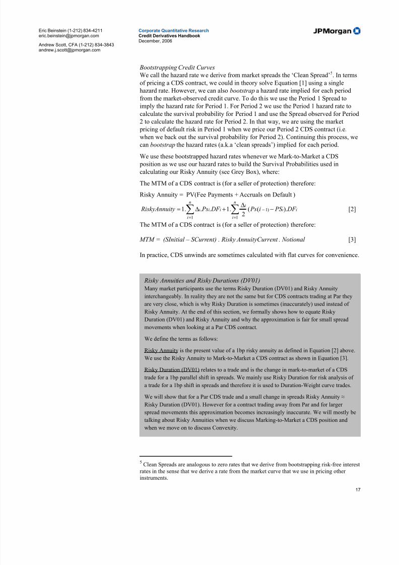
Bootstrapping Credit Curves
We call the hazard rate we derive from market spreads the ‘Clean Spread’5. In terms
of pricing a CDS contract, we could in theory solve Equation [1] using a single
hazard rate. However, we can also bootstrap a hazard rate implied for each period
from the market-observed credit curve. To do this we use the Period 1 Spread toimply the hazard rate for Period 1. For Period 2 we use the Period 1 hazard rate to
calculate the survival probability for Period 1 and use the Spread observed for Period
2 to calculate the hazard rate for Period 2. In that way, we are using the market
pricing of default risk in Period 1 when we price our Period 2 CDS contract (i.e.
when we back out the survival probability for Period 2). Continuing this process, we
can bootstrap the hazard rates (a.k.a ‘clean spreads’) implied for each period.
We use these bootstrapped hazard rates whenever we Mark-to-Market a CDS
position as we use our hazard rates to build the Survival Probabilities used in
calculating our Risky Annuity (see Grey Box), where:
The MTM of a CDS contract is (for a seller of protection) therefore:
Risky Annuity = PV(Fee Payments + Accruals on Default )
∑∑=
−
=
−∆
+∆≈
n
i
iii
n
i
iii DF PS i Ps DF Psty RiskyAnnui
1
)1
1
).((2
.1...1 [2]
The MTM of a CDS contract is (for a seller of protection) therefore:
MTM = (SInitial – SCurrent) . Risky AnnuityCurrent . Notional [3]
In practice, CDS unwinds are sometimes calculated with flat curves for convenience.
5Clean Spreads are analogous to zero rates that we derive from bootstrapping risk-free interest
rates in the sense that we derive a rate from the market curve that we use in pricing other instruments.
Risky Annuities and Risky Durations (DV01)
Many market participants use the terms Risky Duration (DV01) and Risky Annuity
interchangeably. In reality they are not the same but for CDS contracts trading at Par they
are very close, which is why Risky Duration is sometimes (inaccurately) used instead of
Risky Annuity. At the end of this section, we formally shows how to equate Risky
Duration (DV01) and Risky Annuity and why the approximation is fair for small spread
movements when looking at a Par CDS contract.
We define the terms as follows:
Risky Annuity is the present value of a 1bp risky annuity as defined in Equation [2] above.
We use the Risky Annuity to Mark-to-Market a CDS contract as shown in Equation [3].
Risky Duration (DV01) relates to a trade and is the change in mark-to-market of a CDS
trade for a 1bp parallel shift in spreads. We mainly use Risky Duration for risk analysis of
a trade for a 1bp shift in spreads and therefore it is used to Duration-Weight curve trades.
We will show that for a Par CDS trade and a small change in spreads Risky Annuity ≈
Risky Duration (DV01). However for a contract trading away from Par and for larger
spread movements this approximation becomes increasingly inaccurate. We will mostly be
talking about Risky Annuities when we discuss Marking-to-Market a CDS position and
when we move on to discuss Convexity.
5/10/2018 JPM Credit Derivatives - slidepdf.com
http://slidepdf.com/reader/full/jpm-credit-derivatives-559e0102dc371 18/180
Eric Beinstein (1-212) [email protected]
Andrew Scott, CFA (1-212) [email protected]
Corporate Quantitative ResearchCredit Derivatives HandbookDecember, 2006
18
The Shape of Credit Curves
The concepts of Survival Probability, Default Probability and Hazard Rates that we
have seen so far help us to price a CDS contract and also to explain the shape of
credit curves.
Why do many CDS curves slope upwards?
The answer many would give to this is that investors demand greater compensation,
or Spread, for giving protection for longer periods as the probability of defaulting
increases over time. However, whilst it's true that the cumulative probability of
default does increase over time, this by itself does not imply an upward sloping credit
curve – flat or even downward sloping curves also imply the (cumulative) probability
of default increasing over time. To understand why curves usually slope upwards, we
will first look at what flat spread curves imply.
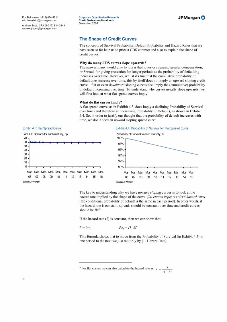
What do flat curves imply?
A flat spread curve, as in Exhibit 4.3, does imply a declining Probability of Survival
over time (and therefore an increasing Probability of Default), as shown in Exhibit4.4. So, in order to justify our thought that the probability of default increases with
time, we don’t need an upward sloping spread curve.
Exhibit 4.3: Flat Spread Curve
Par CDS Spreads for each maturity, bp
0
10
20
30
40
50
60
70
Mar-
06
Mar-
07
Mar-
08
Mar-
09
Mar-
10
Mar-
11
Mar-
12
Mar-
13
Mar-
14
Mar-
15
Mar-
16 Source: JPMorgan
Exhibit 4.4: Probability of Survival for Flat Spread Curve
Probability of Survival to each maturity, %
90%
92%
94%
96%
98%
100%
Mar-
06
Mar-
07
Mar-
08
Mar-
09
Mar-
10
Mar-
11
Mar-
12
Mar-
13
Mar-
14
Mar-
15 Source: JPMorgan
The key to understanding why we have upward sloping curves is to look at the
hazard rate implied by the shape of the curve: flat curves imply constant hazard rates
(the conditional probability of default is the same in each period). In other words, if
the hazard rate is constant, spreads should be constant over time and credit curves
should be flat6.
If the hazard rate ( λ) is constant, then we can show that:
For i=n, Psn = (1- λ )n
This formula shows that to move from the Probability of Survival (in Exhibit 4.5) in
one period to the next we just multiply by (1- Hazard Rate).
6For flat curves we can also calculate the hazard rate as:
R)-(1
S =λ

5/10/2018 JPM Credit Derivatives - slidepdf.com
http://slidepdf.com/reader/full/jpm-credit-derivatives-559e0102dc371 19/180
Eric Beinstein (1-212) [email protected]
Andrew Scott, CFA (1-212) [email protected]
Corporate Quantitative ResearchCredit Derivatives HandbookDecember, 2006
19
So what does an upward-sloping curve imply?
For curves to slope upwards, we need the hazard rate to be increasing over time.
Intuitively, this means that the probability of defaulting in any period (conditional on
not having defaulted until then) increases as time goes on. Upward sloping curves
mean that the market is implying not only that companies are more likely to defaultwith every year that goes by, but also that the likelihood in each year is ever
increasing. Credit risk is therefore getting increasingly worse for every year into the
future7.
An upward sloping curve, such as in Exhibit 4.1, implies a survival probability as
shown in Exhibit 4.5, which declines at an increasing rate over time. This means that
we have an increasing hazard rate for each period as shown in Exhibit 4.6.
Exhibit 4.5: Probability of Survival for Upward Sloping Spread Curve
Probability of Survival to each maturity, %
40%
50%
60%
70%
80%90%
100%
Mar-
06
Mar-
07
Mar-
08
Mar-
09
Mar-
10
Mar-
11
Mar-
12
Mar-
13
Mar-
14
Mar-
15 Source: JPMorgan
Exhibit 4.6: Hazard Rates for Upward Slo ping Spread Curve
Conditional probability of default in each period, %
0.00%
1.00%
2.00%
3.00%4.00%
5.00%
Mar-
06
Mar-
07
Mar-
08
Mar-
09
Mar-
10
Mar-
11
Mar-
12
Mar-
13
Mar-
14
Mar-
15
Source: JPMorgan
As Exhibit 4.6 illustrates, we tend to model hazard rates as a step function, meaning
we hold them constant between changes in spreads. This means that we will haveconstant hazard rates between every period, which will mean Flat Forwards, or
constant Forward Spreads between spread changes. This can make a difference in
terms of how we look at Forwards and Slide.
Downward sloping credit curves
Companies with downward sloping curves have decreasing hazard rates, as can be
seen when looking at GMAC (see Exhibit 4.7). This does not mean that the
cumulative probability of default decreases, rather it implies a higher conditional
probability of default (hazard rate) in earlier years with a lower conditional
probability of default in later periods (see Exhibit 4.8). This is typically seen in lower
rated companies where there is a higher probability of default in each of the
immediate years. But if the company survives this initial period, then it will be in
better shape and less likely to (conditionally) default over subsequent periods.
7One explanation justifying this can be seen by looking at annual company transition
matrices. Given that default is an 'absorbing state' in these matrices, companies will tend todeteriorate in credit quality over time. The annual probability of default increases for eachrating state the lower we move, and so the annual probability of default increases over time.

5/10/2018 JPM Credit Derivatives - slidepdf.com
http://slidepdf.com/reader/full/jpm-credit-derivatives-559e0102dc371 20/180
Eric Beinstein (1-212) [email protected]
Andrew Scott, CFA (1-212) [email protected]
Corporate Quantitative ResearchCredit Derivatives HandbookDecember, 2006
20
Exhibit 4.7: Downward Sloping Par CDS Spreads
GMAC Curve, bp
300
350
400
450
500
Feb-
06
Feb-
07
Feb-
08
Feb-
09
Feb-
10
Feb-
11
Feb-
12
Feb-
13
Feb-
14
Feb-
15
Feb-
16 Source: JPMorgan
Exhibit 4.8: Boot strapped Hazard Rates
%
3.20%
3.40%
3.60%
3.80%
4.00%
Feb-
06
Feb-
07
Feb-
08
Feb-
09
Feb-
10
Feb-
11
Feb-
12
Feb-
13
Feb-
14
Feb-
15
Feb-
16
Source: JPMorgan
Having seen what the shape of credit curves tells us, we now move on to look at how
we calculate Forward Spreads using the curve.
Forwards in credit
Forward rates and their meaning
In CDS, a Forward is a CDS contract where protection starts at a point in the future
(‘forward starting’). For example, a 5y/5y Forward is a 5y CDS contract starting in
five years8. The Forward Spread is then the fair spread agreed upon today for
entering into the CDS contract at a future date.
The Forward is priced so that the present value of a long risk 5y/5y Forward trade is
equivalent to the present value of selling protection for 10y and buying protection for
5y, where the position is default neutral for the first five years and long credit risk for
the second five years, as illustrated in Exhibit 4.9.
Exhibit 4.9: Forward Cashflows For Long Risk 5y/5y Forward
Spreads, bp
S5y
S10y
S5y/5y
Source: JPMorgan
Deriving the forward equationThe Forward Spread is struck so that the present value of the forward starting
protection is equal to the present value of the 10y minus 5y protection.
Given that the default protection of these positions is the same (i.e. no default risk for
the first 5 years and long default risk on the notional for the last 5y), the present
value of the fee legs must be equal as well. We can think of the Forward as having
sold protection for 10y at the Forward Spread and bought protection for 5y at the
8See also, Credit Curves and Forward Spreads (J. Due, May 2004).

5/10/2018 JPM Credit Derivatives - slidepdf.com
http://slidepdf.com/reader/full/jpm-credit-derivatives-559e0102dc371 21/180
Eric Beinstein (1-212) [email protected]
Andrew Scott, CFA (1-212) [email protected]
Corporate Quantitative ResearchCredit Derivatives HandbookDecember, 2006
21
Forward Spread. The fee legs on the first five years net out, meaning we are left with
a forward-starting annuity.
Given that the present value of a 10y annuity (notional of 1) = S 10y . A10y
Where ,S 10y = The Spread for a 10 year CDS contract
A10y = The Risky Annuity for a 10 year CDS contract
We can write:
S 10y . A10y – S 5y . A5y = S 5y/5y . A10y – S 5y/5y . A5y
Where ,
21, t t S = Spread on t2-t1 protection starting in t1 years’ time
Solving for the Forward Spread:
y y
y y y y y y
A A
AS AS S
510
5510105/5
..
−
−=
For example, Exhibit 4.10 shows a 5y CDS contract at 75bp (5y Risky Annuity is
4.50) and a 10y CDS contract at 100bp (10y Risky Annuity is 8.50).
The Forward Spread = bp1285.45.8
)5.475()5.8100(=
−
×−×
Exhibit 4.10: 5y/5y Forward Calcul ations
5y 10y
Spread (bp) 75 100Risky Annuity 4.5 8.5
5y/5yForward Spread (bp) 128
Source: JPMorgan
For a flat curve, Forward Spread = Par Spread, as the hazard rate over any period is
constant meaning the cost of forward starting protection for a given horizon length
(i.e. five years) is the same as protection starting now for that horizon length. We can
show that this is the case for flat curves, since S t2 = S t1= S :
S A AS
A A
AS AS S
t t
t t
t t
t t t t
t t =−
−
=−
−
=12
12
12
1.12.2
21
).(,
We refer to an equal-notional curve trade as a Forward, as the position is present
value equivalent to having entered a forward-starting CDS contract. To more closely
replicate the true Forward we must strike both legs at the Forward Spread. In
practice, an equal-notional curve trade for an upward-sloping curve (e.g. sell 10y
protection, buy 5y protection on equal notionals) will have a residual annuity
cashflow as the 10y spread will be higher than the 5y. Market practice can be to
strike both legs with a spread equal to one of the legs and to have an upfront payment
(the risky present value of the residual spread) so that there are no fee payments in
the first 5 years. In that sense, replicating the Forward with 5y and 10y protection is

5/10/2018 JPM Credit Derivatives - slidepdf.com
http://slidepdf.com/reader/full/jpm-credit-derivatives-559e0102dc371 22/180
Eric Beinstein (1-212) [email protected]
Andrew Scott, CFA (1-212) [email protected]
Corporate Quantitative ResearchCredit Derivatives HandbookDecember, 2006
22
not truly ‘forward starting’ as there needs to be some payment before five years and
protection on both legs starts immediately.
What do forward rates actually look like?
When we model forward rates in credit we use Flat Forwards meaning we keep theforward rate constant between spread changes (see Exhibit 4.11). This is a result of
the decision to use constant (flat) hazard rates between each spread change.
This can be important when we look at the Slide in our CDS positions (and curve
trades) which we discuss in Section 10.
Exhibit 4.11: Par CDS Spreads and 1y Forward Spreads
bp
0
50
100150
200
250
300
0 1 2 3 4 5 6 7 8 9 10
Spread
1Y Forward
Source: JPMorgan
Summary
We have seen how we can understand the shape of the credit curve and how this
relates to the building blocks of default probabilities and hazard rates. These
concepts will form the theoretical background as we discuss our framework for
analyzing curve trades using Slide, Duration-Weighting and Convexity in Section 10.

5/10/2018 JPM Credit Derivatives - slidepdf.com
http://slidepdf.com/reader/full/jpm-credit-derivatives-559e0102dc371 23/180
Eric Beinstein (1-212) [email protected]
Andrew Scott, CFA (1-212) [email protected]
Corporate Quantitative ResearchCredit Derivatives HandbookDecember, 2006
23
Risky Annuities and Risky Durations (DV01)
We show how to accurately treat Risky Annuity and Risky Duration (DV01) and the
relationship between the two. We define Risky Annuity and Risky Duration (DV01)
as follows: Risky Annuity is the present value of a 1bp risky annuity stream:
∑∑=
−
=
−∆
+∆≈=
n
i
iiii
n
i
iii s DF PS Ps DF Ps Aty RiskyAnnui
1
1
1
).(2
.1...1
where A s = Risky Annuity for an annuity lasting n periods, given spread
level S
Risky Duration (DV01) relates to a trade and is the change in mark-to-market of a
CDS trade for a 1bp parallel shift in spreads.
The Mark-to-Market for a long risk CDS trade using Equation [3], (Notional = 1) is:
MTMScurrent= (SInitial – SCurrent) . AScurrent
MTM 1bp shift = (S Initial – S Current +1bp ) . AS current
+1bp
Given, DV01 (Risky Duration) = MTM 1bp shift - MTM S current
DV01 = [ (S Initial – S Current +1bp ) . AS current
+1bp
] – [(S Initial – S Current ) . AS current
]
Using,
S Current +1bp . AS current
+1bp
= S Current . AS current
+1bp
+ 1bp . AS current
+1bp
We can show that:
DV01 = - A S current
+1bp
+ (S Initial – S Current ) .( A S current
+1bp
- A S current
)
For a par trade S Initial = S Current , and since Risky Annuities do not change by a large
amount for a 1bp change in Spread, we get:
DV01 = - A Scurrent +1bp ≈- A Scurrent I.e. Risky Duration ≈ Risky Annuity
This approximation can become inaccurate if we are looking at a trade that is far off-
market, where S Initial – S Current becomes significant, causing the Risky Duration to
move away from the Risky Annuity.
Also, as we start looking at spread shifts larger than 1bp, the shifted Risky Annuity
will begin to vary more from the current Risky Annuity (a Convexity effect) and
therefore we need to make sure we are using the correct Risky Annuity to Mark-to-
Market and not the Risky Duration (DV01) approximation.
5/10/2018 JPM Credit Derivatives - slidepdf.com
http://slidepdf.com/reader/full/jpm-credit-derivatives-559e0102dc371 24/180
Eric Beinstein (1-212) [email protected]
Andrew Scott, CFA (1-212) [email protected]
Corporate Quantitative ResearchCredit Derivatives HandbookDecember, 2006
24
5. The ISDA Agreement
Standardized documentation
The standardization of documentation from the International Swaps and DerivativesAssociation (ISDA) has been an enormous growth driver for the CDS market.
ISDA produced its first version of a standardized CDS contract in 1999. Today, CDSis usually transacted under a standardized short-form letter confirmation, whichincorporates the 2003 ISDA Credit Derivatives Definitions, and is transacted under the umbrella of an ISDA Master Agreement9. Combined, these agreements address:
• Which credit, if they default, trigger the CDS
• The universe of obligations that are covered under the contract
• The notional amount of the default protection
• What events trigger a credit event
• Procedures for settlement of a credit event
Standardized confirmation and market conventions mean that the parties involvedneed only to specify the terms of the transaction that inherently differ from trade totrade (e.g., reference entity, maturity date, spread, notional). Transactional ease isincreased because CDS participants can unwind a trade or enter an equivalentoffsetting contract with a different counterparty from whom they initially traded. Asis true with other derivatives, CDS that are transacted with standard ISDAdocumentation may be assigned to other parties. In addition, single-name CDScontracts mature on standard quarterly end dates. These two features have helped promote liquidity and, thereby, stimulate growth in the CDS market.
ISDA’s standard contract has been put to the test and proven effective in the face of significant credit market stress. With WorldCom and Parmalat filing for bankruptcyin 2002 and 2003, respectively, and more recently Delphi Corp, Dana Corp, CalpineCorp, Northwest and Delta airlines filing in 2005 and 2006, the market has seenthousands of CDS contracts and over $50 billion of notional outstanding settle postdefault. In all situations of which we are aware, contracts were settled withoutoperational settlement problems, disputes or litigation.
The new CDS settlement protocol
The current CDS contract is based on the 2003 ISDA definitions and calls for
physical settlement following a credit event, as described in Section 2. An
alternative settlement mechanism known as the CDS protocol has been developed by
ISDA in conjunction with the dealer community, however. The new settlement protocol allows investors to cash or physically settle contracts at a recovery rate
determined in an auction process. A protocol was first introduced after Collins &
Aikman defaulted then refined for the Delphi Corp. and Calpine Corp. credit events.
The settlement protocol can be used to settle:
• Single name CDS contracts
9For more information on the ISDA standard definitions, see ‘The 2003 ISDA Credit
Derivatives Definitions’ note published on June 13, 2003 by Jonathan Adams and TomBenison.
5/10/2018 JPM Credit Derivatives - slidepdf.com
http://slidepdf.com/reader/full/jpm-credit-derivatives-559e0102dc371 25/180
Eric Beinstein (1-212) [email protected]
Andrew Scott, CFA (1-212) [email protected]
Corporate Quantitative ResearchCredit Derivatives HandbookDecember, 2006
25
• Credit derivative indices and tranched indices, including the CDX, TRAC-X, and HYDI
• Bespoke portfolio transactions
• Other CDS transactions, including Constant Maturity Swaps, Principal OnlyTransactions, Interest Only Transactions, Nth to Default Transactions,Recovery Lock Transactions, and Portfolio Swaptions
Note that the Protocol is optional and not part of the 2003 ISDA definitions.
Summary of CDS Protocol
• The protocol effectively allows investors to cash or physically settle their CDScontracts using a Recovery Rate determined in an auction process.
• The timing of the settlement of contracts using the Protocol mirrors the timingof settlement without using the Protocol. Namely, a bond auction will occur approximately 30 days after the credit event, and contracts will settle shortlythereafter.
• Following a credit event, ISDA will publish a Settlement Protocol for thedefaulted credit. The Protocol will have a timeline of events and list of obligations that can be delivered into the contract. Once the Protocol is
published, investors decide whether to opt-in. Note that after opting in,investors retain the ability to unwind their trade and pay/receive 100% -recovery, where recovery is the price of the defaulted bond in the open market.This is common practice as credit default swaps are bilateral agreements between two parties. Investors can unwind their positions up until the day before the auction.
• By the day of the auction, investors must decide if they want to [1] cash or [2]
physically settle their net positions through the auction. Namely, investorshave the option to [1] cash settle and pay/receive 100 – Recovery Rate, or [2]
physically settle, trading bonds at the final Recovery Rate determined in theauction. Investors may trade a bond position as large as their net CDS position.To physically settle, investors must alert their dealers. We suggest calling theday before the auction, and re-confirming on the morning of the auction.
• The CDS protocol auction has two parts. In part one, two numbers arecalculated.
• Part 1a) Dealers submit bid/ask prices for bonds to the auction Administrator and a midpoint is calculated. This midpoint can be thought of as thepreliminary Recovery Rate.
• Part 1b) Second, the Administrator calculates the Open Interest. Open Interestis created when a protection buyer wishes to physically settle but the protectionseller does not, or visa-versa. If all CDS contract holders cash settle or if allholders physically settle, as there is a protection buyer for every seller (assumingall investors opt into the Protocol), Open Interest must be zero, by definition. Itis only created when, for example, a protection seller (long risk) wishes to physically settle a $10 million contract at the market clearing price, but the protection buyer does not. Open Interest of $10 million to buy bonds would becreated. We explain the intuition behind the “buy” order in the Mechanicssection.
• Limit orders submitted: After the Administrator calculates and posts the
results of Part 1 on its website, dealers and clients working through their dealers have approximately two hours to submit limit orders to buy or sell bonds, depending on the Open Interest direction. This is a new feature not

5/10/2018 JPM Credit Derivatives - slidepdf.com
http://slidepdf.com/reader/full/jpm-credit-derivatives-559e0102dc371 26/180
Eric Beinstein (1-212) [email protected]
Andrew Scott, CFA (1-212) [email protected]
Corporate Quantitative ResearchCredit Derivatives HandbookDecember, 2006
26
included in previous protocols. In our example, only limit orders to sell bondswould be submitted in order to satisfy the $10 million Open Interest to buy bonds calculated in Part 1. Note that any investor can submit limit orders(working through their dealers), whether they are involved in CDS or not. In
our opinion, this is the best opportunity for investors to express their viewson Recovery Rate.
• Part 2 of the auction is a Dutch Auction where the Open Interest is filled usinglimit orders. The price of the final limit order used to fill the Open Interest
will be the final Recovery Rate. This Recovery Rate is used to cash and
physically settle contracts, and is the price at which all limit orders transact.The transactions will occur shortly after the auction.
Ultimately, we expect a future iteration of the settlement Protocol to be incorporatedinto the standard ISDA credit default swap documentation. If and when this occurs,the new documentation would likely require adherence to these settlement terms.Furthermore, outstanding CDS contracts may be able to opt into a Protocol as well,so that all outstanding CDS contracts would settle in the same manner. The market
will address these issues in turn. Exhibit 5.1: Summary of the CDS Protocol. Note, timeline is hypothetical and will be determined after a credit event
HypotheticalTimeline
Protocol mechanic Client decisions
Default
CDS Protocol taken off "shelf" and published for defaulted credit with list of Deliverable Obligations.
Do I opt-into the protocol?
Do I unwind my CDS trade pre-auction?
Default +27 Final day to unwind CDS trades, if opted in.
Default +28 Auction Part 1A: initial Recovery Rate determined through dealer fixing and published
Auction Part 1B: Market Orders collected and Open Interest calculated and published Do I want to physically settle my CDS contract? If yes, submitMarket Order, potentially creating Open Interest. If not, will cashsettle.
For 2 hours, limit bids or offers collected, as appropriate based on Open Interest Do I want to submit limit orders for bonds?
Auction Part 2: Dutch auction, determination of final Recovery Rate
Default +30 Delivery of Notice of Physical Settlement for clients who elected to trade bonds inauction.
If I sold bonds in auction, what bonds will I deliver?
Default +33 Settlement of bonds traded in auction
Default +40 Settlement of all trades, cash and physical
Source: JPMorgan

5/10/2018 JPM Credit Derivatives - slidepdf.com
http://slidepdf.com/reader/full/jpm-credit-derivatives-559e0102dc371 27/180
Eric Beinstein (1-212) [email protected]
Andrew Scott, CFA (1-212) [email protected]
Corporate Quantitative ResearchCredit Derivatives HandbookDecember, 2006
27
CDS Protocol auction example Part 1.A: initial recovery rate calculationDealers submit bids/offers to the Administrator which are sorted (Exhibit 2). Ordersthat are tradable are set aside, meaning bids and offers are set aside when bids match
offers or if bids are greater than offers. The best 50% of remaining bids and offersare averaged. The initial recovery rate is 65.75%.
Exhibit 5.2: Part 1.A of auction. Dealers submit bids/offers for bonds based on market trading levels.
Bids/Offers are sorted, and tradable markets and initial Recovery Rate are determined.
Initial submissions Sorted submissions
Dealer Bid Offer Bid Offer
1 $65.00 $67.00 $68.00 $64.00
2 $64.00 $66.00 $67.00 $65.00 Tradeable
3 $63.00 $65.00 $67.00 $66.00 markets
4 $67.00 $69.00 $66.00 $66.00
5 $62.00 $64.00 $65.00 $66.00 Best half of non-tradable markets
6 $65.00 $67.00 $65.00 $67.00 Average, initial Recovery Rate = $65.757 $64.00 $66.00 $65.00 $67.00
8 $66.00 $68.00 $64.00 $67.00
9 $65.00 $67.00 $64.00 $68.00
10 $64.00 $66.00 $64.00 $69.00
11 $67.00 $69.00 $63.00 $69.00
12 $68.00 $70.00 $62.00 $70.00
Source: JPMorgan Source: JPMorgan
Part 1.B: Open Interest calculationThe orders to physically settle bonds at the market clearing price are aggregated bythe Administrator. In our example, there is a $100 million face value net demand to buy bonds at the market clearing price (Exhibit 3).
Exhibit 5.3 Part 1.B of auction: Open Interest is calculated
Buy Market Orders Sell Market Orders
(bond face value MM) (bond face value MM)
$500 $400
Open Interest: $100
Source: JPMorgan
Part 2: Dutch Auction and determination of final Recovery RateThe Recovery Rate and Open Interest calculated in Part 1 are published to themarket. Investors have two hours to submit limit orders to their dealers. The limitorders to sell bonds are aggregated by the Administrator. The $100 million of
market orders are filled by all of the limit orders, starting with $64, and finishing at$68 (Exhibit 4). Thus, $900 million of market orders for bonds, and $100 million of limit orders used to fill the market orders will trade at $68. These bonds will actuallytrade. Furthermore, all credit default swap contracts signed up for the protocol willcash settle with a recovery rate of 68%. Thus, buyers of protection (short risk) willreceive $32 (100-68) per $100 of notional risk, paid by the sellers of protection (longrisk).
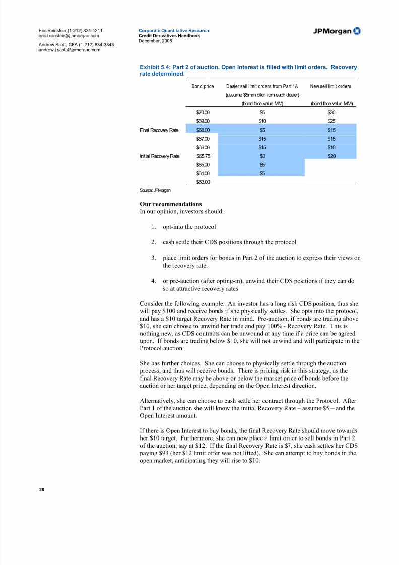
5/10/2018 JPM Credit Derivatives - slidepdf.com
http://slidepdf.com/reader/full/jpm-credit-derivatives-559e0102dc371 28/180
Eric Beinstein (1-212) [email protected]
Andrew Scott, CFA (1-212) [email protected]
Corporate Quantitative ResearchCredit Derivatives HandbookDecember, 2006
28
Exhibit 5.4: Part 2 of auction. Open Interest is filled with limit orders. Recoveryrate determined.
Bond price Dealer sell limit orders from Part 1A New sell limit orders
(assume $5mm offer from each dealer)
(bond face value MM) (bond face value MM)
$70.00 $5 $30
$69.00 $10 $25
Final Recovery Rate $68.00 $5 $15
$67.00 $15 $15
$66.00 $15 $10
Initial Recovery Rate $65.75 $0 $20
$65.00 $5
$64.00 $5
$63.00
Source: JPMorgan
Our recommendationsIn our opinion, investors should:
1. opt-into the protocol
2. cash settle their CDS positions through the protocol
3. place limit orders for bonds in Part 2 of the auction to express their views on
the recovery rate.
4. or pre-auction (after opting-in), unwind their CDS positions if they can do
so at attractive recovery rates
Consider the following example. An investor has a long risk CDS position, thus shewill pay $100 and receive bonds if she physically settles. She opts into the protocol,and has a $10 target Recovery Rate in mind. Pre-auction, if bonds are trading above$10, she can choose to unwind her trade and pay 100% - Recovery Rate. This isnothing new, as CDS contracts can be unwound at any time if a price can be agreedupon. If bonds are trading below $10, she will not unwind and will participate in theProtocol auction.
She has further choices. She can choose to physically settle through the auction process, and thus will receive bonds. There is pricing risk in this strategy, as thefinal Recovery Rate may be above or below the market price of bonds before theauction or her target price, depending on the Open Interest direction.
Alternatively, she can choose to cash settle her contract through the Protocol. After Part 1 of the auction she will know the initial Recovery Rate – assume $5 – and theOpen Interest amount.
If there is Open Interest to buy bonds, the final Recovery Rate should move towardsher $10 target. Furthermore, she can now place a limit order to sell bonds in Part 2of the auction, say at $12. If the final Recovery Rate is $7, she cash settles her CDS paying $93 (her $12 limit offer was not lifted). She can attempt to buy bonds in theopen market, anticipating they will rise to $10.

5/10/2018 JPM Credit Derivatives - slidepdf.com
http://slidepdf.com/reader/full/jpm-credit-derivatives-559e0102dc371 29/180
Eric Beinstein (1-212) [email protected]
Andrew Scott, CFA (1-212) [email protected]
Corporate Quantitative ResearchCredit Derivatives HandbookDecember, 2006
29
If the final Recovery Rate is $15, she cash settles her CDS paying $85, and also sells bonds at $15 (not $12, but the final RR), perhaps selling short. She anticipatescovering her short in the open market closer to $10.
The opposite situation holds for a short risk CDS investor. Thus, the Protocol helpsseparate the investment decisions of unwinding the CDS contract and taking a viewon Recovery Rates. This could help to minimize the volatility of bond prices, as the bonds should trade to the market consensus Recovery Rate. This Rate should reflectthe fundament value of the defaulted bonds.
Protocol goalsAt the beginning of 2006, ISDA discussed multiple goals for the Protocol:
1. Reduce the price volatility of defaulted bonds caused by the settlement of CDS
contracts.
2. Ensure that, if CDS contracts were used to hedge bond positions, bonds can be
traded at the same price as the Recovery Rate determined in an auction.
3. Simplify CDS settlement logistics.
4. Use one recovery rate for all CDS contracts. This allows index positions hedged
with single name CDS to settle using the same recovery rate, for example, and
tranche contracts to remain fungible.
Unfortunately, goals [1] and [2] are conflicting. A cash settlement process can solveissue [1]. Specifically, the credit default swap market is a closed system, as there is a buyer of protection for every seller. If the market agreed on a recovery rate, all CDScontracts could be settled using this rate, and artificial demand for bonds caused byCDS contract settlement would be avoided. However, issue [2] would remainunsolved. Namely, investors who purchased bonds (long risk) and CDS protection(short risk) would cash settle their CDS position and receive (1 – recovery rate
percentage) through the auction. They might not be able to sell the bond they own atthis rate in the open market, however. Thus, these bond and protection owners could be exposed to discrepancies in recovery rate.
Issue [2] is addressed through physical settlement, for in this process, the price paidfor the bond is the recovery rate, by definition. However, if the notional value of outstanding CDS contracts is larger than the face value of deliverable bonds, bond prices may be volatile during the months after default. Buyers of protection couldcause bond prices to rise as they purchase bonds needed to settle their contracts,amplifying issue [1].
The ISDA proposal attempts to optimize a solution given the competing priorities. Inour opinion, the two step auction process does this. This could help to minimize the
volatility of bond prices, as the bonds should trade to the market consensus RecoveryRate. This Rate should reflect the fundamental value of the defaulted bonds.
Exhibit 5.5: History of open interest in auctions. In the three Dutch Auctions,protection buyers have physically settled, creating Open Interest to sell bonds
Credit Date of auction Open Interest ($mm) Open Interest direction Recovery Rate
Dana Corp 03/31/2006 41 Sell bonds 75.0%
Calpine Corp 01/17/2006 45 Sell bonds 19.125%
Delphi Corp 11/04/2005 99 Sell bonds 63.375%
Source: JPMorgan

5/10/2018 JPM Credit Derivatives - slidepdf.com
http://slidepdf.com/reader/full/jpm-credit-derivatives-559e0102dc371 30/180
Eric Beinstein (1-212) [email protected]
Andrew Scott, CFA (1-212) [email protected]
Corporate Quantitative ResearchCredit Derivatives HandbookDecember, 2006
30
Protocol MechanicsInvestors choose to participate in the protocol by emailing a signed adherence letter to ISDA. Even after opted in, investors can continue to unwind or settle trades up tothe day before the auction. After this date, investors must settle using the mechanics
described by the Protocol.
Under the 2003 ISDA definitions, CDS investors were required to fax individualnotices to each of their counterparties. No notices need to be delivered under theProtocol for trades covered by the Protocol. If notices happened to be delivered before investors sign up for a Protocol, the notices are revoked. By adopting theProtocol investors agree that the credit event occurred on the date specified in theProtocol, and that CDS coupons accrue up to and including the credit event date(called the Event Determination Date). The date of the credit event is typicallyrecorded as the day of the event if the credit event occurs before noon, and the dayafter if not.
There are two parts to the auction.
Part 1: Initial Recovery Rate and Open Interest calculationThere are two goals in the Initial Bidding process. First, to determine an initialrecovery rate through a dealer fixing process and second, to determine the netdemand/supply of bonds created by investors wishing to physically settle their netCDS positions.
1.A) Initial Market Midpoint, or the preliminary Recovery Rate calculationDealers submit bid/ask markets to the Administrator, with a maximum bid/ask spreadof 2% of par. ISDA will define the size of the bid/ask markets, based on discussionswith market participants and the amount of deliverable obligations outstanding. As a point of reference, $10 million markets were used in previous CDX Protocols. TheAdministrator sorts the best bids and offers. Orders that are tradable effectively
trade, meaning bids and offers trade when bids match offers or if bids are greater than offers (Exhibit 6).
Exhibit 5.6: Part 1A of auction – dealers submit bids/offers to Administrator
Contributed Sorted
IM Bids IM Offers IM Bids IM Offers
39.50% 41.00% 45.00% 34.00%
40.00% 42.00% 41.00% 39.50%
41.00% 43.00% 41.00% 40.00%
45.00% 47.00%Best half
40.00% 41.00%
32.00% 34.00%of non-
Tradable39.50% 42.00%
38.75% 40.00%Markets
38.75% 42.75%
38.00% 39.50% 38.00% 43.00%
41.00% 42.75% 32.00% 47.00%
Source: ISDA CDS Protocol
TradableMarkets
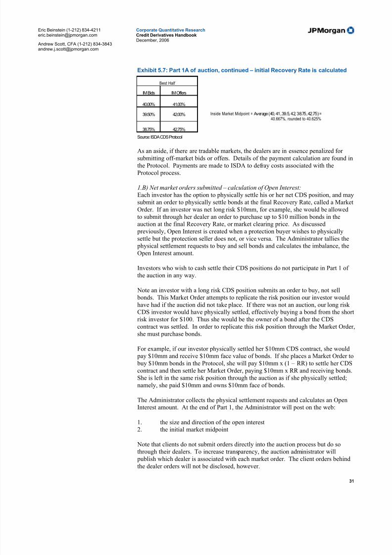
5/10/2018 JPM Credit Derivatives - slidepdf.com
http://slidepdf.com/reader/full/jpm-credit-derivatives-559e0102dc371 31/180
Eric Beinstein (1-212) [email protected]
Andrew Scott, CFA (1-212) [email protected]
Corporate Quantitative ResearchCredit Derivatives HandbookDecember, 2006
31
Exhibit 5.7: Part 1A of auction, continued – initial Recovery Rate is calculated
Best Half
IM Bids IM Offers
40.00% 41.00%
39.50% 42.00% Inside Market Midpoint = Average (40, 41, 39.5, 42, 38.75, 42.75) =40.667%, rounded to 40.625%
38.75% 42.75%
Source: ISDA CDS Protocol
As an aside, if there are tradable markets, the dealers are in essence penalized for submitting off-market bids or offers. Details of the payment calculation are found inthe Protocol. Payments are made to ISDA to defray costs associated with theProtocol process.
1.B) Net market orders submitted – calculation of Open Interest:
Each investor has the option to physically settle his or her net CDS position, and maysubmit an order to physically settle bonds at the final Recovery Rate, called a MarketOrder. If an investor was net long risk $10mm, for example, she would be allowedto submit through her dealer an order to purchase up to $10 million bonds in theauction at the final Recovery Rate, or market clearing price. As discussed previously, Open Interest is created when a protection buyer wishes to physicallysettle but the protection seller does not, or vice versa. The Administrator tallies the physical settlement requests to buy and sell bonds and calculates the imbalance, theOpen Interest amount.
Investors who wish to cash settle their CDS positions do not participate in Part 1 of the auction in any way.
Note an investor with a long risk CDS position submits an order to buy, not sell bonds. This Market Order attempts to replicate the risk position our investor wouldhave had if the auction did not take place. If there was not an auction, our long risk CDS investor would have physically settled, effectively buying a bond from the shortrisk investor for $100. Thus she would be the owner of a bond after the CDScontract was settled. In order to replicate this risk position through the Market Order,she must purchase bonds.
For example, if our investor physically settled her $10mm CDS contract, she would pay $10mm and receive $10mm face value of bonds. If she places a Market Order to buy $10mm bonds in the Protocol, she will pay $10mm x (1 – RR) to settle her CDScontract and then settle her Market Order, paying $10mm x RR and receiving bonds.She is left in the same risk position through the auction as if she physically settled;
namely, she paid $10mm and owns $10mm face of bonds.
The Administrator collects the physical settlement requests and calculates an OpenInterest amount. At the end of Part 1, the Administrator will post on the web:
1. the size and direction of the open interest2. the initial market midpoint
Note that clients do not submit orders directly into the auction process but do sothrough their dealers. To increase transparency, the auction administrator will publish which dealer is associated with each market order. The client orders behindthe dealer orders will not be disclosed, however.

5/10/2018 JPM Credit Derivatives - slidepdf.com
http://slidepdf.com/reader/full/jpm-credit-derivatives-559e0102dc371 32/180
Eric Beinstein (1-212) [email protected]
Andrew Scott, CFA (1-212) [email protected]
Corporate Quantitative ResearchCredit Derivatives HandbookDecember, 2006
32
If an investor has positions with multiple dealers, she may attempt to submit her totalnet position through one dealer. Per the protocol, the dealer is only required toaccept an order that matches the dealer’s position with the client. The dealer mayaccept the client’s complete order if they choose, or alternatively ask the client to
make submissions through multiple dealers.
Part 2: Dutch auction and final Recovery Rate calculation
The goal of Part 2 is to fill the Open Interest calculated in Part 1B with limit orders.Dealers and clients working through their dealers can place limit orders to buy or sell bonds, depending on the Open Interest calculated. Dealers will have approximatelytwo hours from the announcement of the Part 1 results to submit limit orders to theadministrator.
The Administrator will use the dealer markets from Part 1A of the process andadditional limit orders submitted to fill this demand. The price of the last limit order used to fill the net market orders is the Recovery Rate. It is the price at which thefilled limit orders trade, the price at which market orders for bonds will trade, and it
is the rate used in cash settlement of trades.
If there are not enough limit orders to fill the open interest, the recovery rate will be100% or 0%, if the Open Interests is to buy or sell bonds, respectively. All MarketOrders will then be matched on a pro-rata basis. This situation can only occur if theOpen Interest amount posted in Part 1 does not source enough limit offers. In our opinion, the opportunity to trade distressed bonds in potentially large size at a named price will likely source buyers or sellers during the two hour submission window.
We note a minor detail. If the net market order is to buy bonds, for example, thefinal price determined in the auction cannot be 1% below the midpoint calculated in part [1] of the auction. This unusual situation -- where a buy imbalance settles belowthe midpoint – could only occur if there was small Open Interest that was filled with
sell orders originally submitted in Part 1A by the dealers, sell orders that were at prices below the initial Recovery Rate. This 1% rule prevents an artificially high or low bid/ask submitted in Part 1A from being the final auction price. Conversely, if the net market order is to sell bonds, the final price cannot be 1% above the midpoint.
Other commentsThe Protocol does not currently include Loan Only CDS or Preferred CDS. Weexpect these contracts to adopt the Protocol technology after adjusting it for thespecifics of the contracts.
CDX Note settlement procedures
The settlement procedures for the notes are outlined in the offering memorandum. Note holders do not need to take any action in order for the default to be settled. The
settlement process is as follows:
The CDX dealers will hold the three bond auctions. The CDX dealers deliver bondsto the auction agent over the course of the three auctions. The auction agent then sellsthe bonds to the marketplace through an auction process. The average price paid bythe marketplace during the three auctions will be the recovery price. Note holders inaffected indices then receive a payment of this recovery price.
Coupon paymentsFor current investors in the swap indices, the coupon on the index will include thedefaulted credit and will accrue until the settlement procedure is triggered. Oncetriggered, the defaulted credit will not be included. This will be reflected through a

5/10/2018 JPM Credit Derivatives - slidepdf.com
http://slidepdf.com/reader/full/jpm-credit-derivatives-559e0102dc371 33/180
Eric Beinstein (1-212) [email protected]
Andrew Scott, CFA (1-212) [email protected]
Corporate Quantitative ResearchCredit Derivatives HandbookDecember, 2006
33
change in the notional value of the trade, not in a change in the coupon rate of theindex. For example, the coupon on the DJ CDX.NA.HY.6 is 345bp. If an investor originally purchased $100 of the index, the new notional value of the trade will be$100 * (99/100), or $99, and their coupon payments will be based on this new
notional value.
The coupon on the note index is similar to the swap indices in that the coupon ratedoes not change, but the notional value does. The treatment of the current coupon,however, differs from the swaps. For the note, the next coupon payment will be based on a reduced notional of (99/100) for the entire coupon period.
“Old-fashioned” CDS settlement procedures
Credit default swap contracts have a three-step physical settlement procedure, as per the 2003 ISDA definitions:
1. Notification of a credit eventThe buyer or seller of protection may deliver a notice of a credit event to thecounterparty. Certain public source news articles or a company press release qualifyas official documentation of a credit event. This notice may be legally delivered up to14 days after the maturity of the contract, which may be years after the credit event.
2. Notice of physical settlementOnce the “Notification of a credit event” is delivered, the buyer of protection has 30calendar days to deliver a “Notice of physical settlement.” In this notice, the buyer of protection must specify what bonds or loans they will deliver.
3. Delivery of bondsThe buyer of protection typically delivers bonds to the seller within three days after the “Notice of physical settlement” is submitted. In order to receive full payment,the buyer of protection must deliver bonds with an aggregate face amount equal to
the notional value of the credit exposure that the buyer has. The buyer of protectionmay deliver fewer bonds and receive less cash, if they choose.
5/10/2018 JPM Credit Derivatives - slidepdf.com
http://slidepdf.com/reader/full/jpm-credit-derivatives-559e0102dc371 34/180
Eric Beinstein (1-212) [email protected]
Andrew Scott, CFA (1-212) [email protected]
Corporate Quantitative ResearchCredit Derivatives HandbookDecember, 2006
34
Succession events
A corporate action can cause a Succession Event, or a change in the Reference
Obligation of a CDS contract. Corporate actions can impact bondholders and CDS
investors differently, depending on how the company transaction is structured. In amerger, spin-off or asset sale, for example, companies will often manage their bonds
and loans in a manner that maximizes the company’s economics under the
constraints of debt indentures. While the indentures protect bondholders, they do not
consider CDS investors. CDS are derivatives that do not affect the economics of
companies, thus management teams are not forced to consider the corporate event’s
impact on the contracts. They may consider the contracts, however, as their
bondholders may also use CDS. Thus, the instrument used by the investor, whether
it be bonds or CDS, can make all the difference in whether a corporate action
improves or damages the investor's profit/loss.
Each CDS has a Reference Obligation that defines the issuing entity, or what
company the contract “points” to. In order for the reference obligation of a credit
default swap contract to change, there must be an event that satisfies qualitative andquantitative criteria. The provisions for determining a successor are detailed in the
2003 International Swaps and Derivatives Association (ISDA) Credit Derivatives
Definitions (see www.isda.org for more information).
This note is our interpretation of the ISDA documentation and is not part of the 2003
Definitions. Every corporate action is different, and the facts of the case must be
analyzed. Investors should consult their legal advisors, as appropriate. This report
does not provide legal advice.
Qualitative criteria
The qualitative criteria determines if there is a “Succession Event,” or a corporate
action. Section 2.2(b) of the ISDA definitions describes the event:
"Succession Event" means an event such as a merger, consolidation,
amalgamation, transfer of assets or liabilities, demerger, spin-off or other similar
event in which one entity succeeds to the obligations of another entity, whether
by operation of law or pursuant to any agreement.
This definition should encompass most corporate actions that could affect the debt of
the reference entity. Note that an exchange offer on its own will not constitute a
Succession Event, but must be associated with a corporate action. The definitions
continue:
Notwithstanding the foregoing, "Succession Event " shall not include an event in
which the holders of obligations of the Reference Entity exchange such
obligations for the obligations of another entity, unless such exchange occurs in
connection with a merger, consolidation, amalgamation, transfer of assets or
liabilities, demerger, spin-off or other similar event.
For a corporate event to be a Succession Event, the original entity that was
responsible for servicing the bonds and loans (or Relevant Obligations, to be defined
shortly) must no longer be an obligor or guarantor. Furthermore, a new entity must
assume responsibility for the bonds, either by assuming the liability for the old
bonds, or exchanging the old bonds for new bonds. The new entity is said to
“succeed” to the bonds.

5/10/2018 JPM Credit Derivatives - slidepdf.com
http://slidepdf.com/reader/full/jpm-credit-derivatives-559e0102dc371 35/180
Eric Beinstein (1-212) [email protected]
Andrew Scott, CFA (1-212) [email protected]
Corporate Quantitative ResearchCredit Derivatives HandbookDecember, 2006
35
Finally, note that a corporate name change, redemption or repurchase of debt without
another corporate action, and a change in ownership of stock without a merging of
entities, are not Succession Events.
Quantitative criteriaOnce it is determined that there is a Succession Event using the qualitative criteria, a
Successor(s) may be determined if the quantitative criteria are met. The criteria
reviews how many of the bonds and loans, or Relevant Obligations, are assumed by
another entity. Relevant Obligations include all bonds and loans issued by the
original company, excluding inter-company debt. Note that, in an exchange offer,
the bonds being tendered for may be a subset of the Relevant Obligations. The
percentage calculations use the Relevant Obligations in the denominator, not just the
bonds and loans defined in the exchange. The following rules are used to determine
a Successor:
• If one new entity succeeds to 25% or more of the Relevant Obligations, and
the old company retains less than 25%, the new entity is the sole Successor.
All CDS contracts will reference the new company.
• In the situation described above, if there are multiple new entities that
succeed to 25% or more of the Relevant Obligations, the CDS contracts will
be split equally amongst these new entities. For example, if three new
entities succeeded to 25%, 35% and 40% of the Reference Obligations, a $9
million notional CDS position would be split into three, $3 million positions.
• If the original company retains 25% of the Relevant Obligations, and there
are new entities that succeed to 25% of more of the Obligations, both the new
and original company become Reference Entities. Like in the previous
example, a CDS contract is divided equally between the new Reference
Entities.
• If no entity succeeds to 25% of the Relevant Obligations, and the original
company still exists, there is no Successor and no change to the CDS
contract. If the original company does not exist, the entity that succeeds to
the greatest percentage of the Relevant Obligations becomes the sole
successor.
The Calculation Agent is tasked with making the determination if the qualitative and
quantitative criteria are met. The Calculation Agent is specified in the CDS contract.
Other issues
In a corporate action, the fate of specific bond issues may be different from the fate
of bonds overall and of the credit default swap contracts. For example, if a companytenders for one bond, perhaps because of its pricing or covenants, and leaves another
outstanding, the two bonds may yield different returns. The same holds true for
CDS, which generally follows the aggregate movement of the Relevant Obligations
in a Successor Event, but could yield different profits or losses than the bonds
depending on how the CDS is ultimately divided and the credit quality of the final
Reference Obligations.
Bond guarantees can affect CDS trading levels as well. First, recall that for a
corporate action to be a Succession Event, the original company may no longer be an
obligor or guarantor of the Relevant Obligations. Thus, a guarantee or lack thereof
may determine how many Relevant Obligations succeed, and if an outstanding CDS

5/10/2018 JPM Credit Derivatives - slidepdf.com
http://slidepdf.com/reader/full/jpm-credit-derivatives-559e0102dc371 36/180
Eric Beinstein (1-212) [email protected]
Andrew Scott, CFA (1-212) [email protected]
Corporate Quantitative ResearchCredit Derivatives HandbookDecember, 2006
36
contract will refer to a new entity. Second, for situations with Parent and Subsidiary
companies, guarantees determine which bonds are deliverable to settle CDS contracts
after a credit event. If a Parent guarantees a Subsidiary’s debt, then a CDS contract
with the Parent as the Reference Entity can be settled with debt from the Parent or
Subsidiary, under the standard CDS contracts. The CDS should trade based on thequality of the weaker credit, Parent or Sub. A CDS contract with the Subsidiary as
the Reference Obligation, however, can only be settled with a Subsidiary bond or
loan. Furthermore, upstream guarantees, when a Subsidiary guarantees a Parent’s
bonds, are not considered under the 2003 ISDA definitions. Parent bonds cannot be
used to settle a CDS contract with the Subsidiary as the Reference Obligation.
If all the bonds and loans of a Reference Entity are tendered for, the CDS contract is
not canceled nor does the spread reach zero. The spread should tighten, of course, as
there is less debt and a reduced likelihood that the company defaults. Because the
company retains the option of issuing debt in the future, the CDS should reflect this
likelihood, and the level at which bonds might be issued.
There is a situation in which a CDS contract can be terminated in a Succession event.
If there is a merger between a Reference Entity and the Seller of protection (long
credit risk), the buyer of protection may choose to unwind the trade.
Post-succession, CDS trading logistics
In December 2005, the wireline and wireless telecom company ALLTEL announced
it intention to spin off its wireless business. We use this as an example of the post-
succession trading logistics.
• The spin off was effective on July 17, which is also the effective date of thesuccession event.
• CDS contracts referencing ALLTEL split evenly into two contracts each with
half of the original notional amount, one referencing ALLTEL and the other referencing Windstream, the spin off company. Thus, a $10 million CDSALLTEL contract entered into on or before Friday, July 14 became a $5 millioncontract referencing ALLTEL and a $5 million contract referencing Windstreamon Monday, July 17.
• Legally, CDS contract holders do not need to take any action. A succession eventdoes not require confirmation or acknowledgement from the two contractholders. Thus, CDS contracts do not need to be re-issued.
• The CDS confirmation, 2003 ISDA Credit Derivatives Definitions, and the publicfilings by ALLTEL that allow you to perform the succession event calculations,are the documents that “prove” the occurrence of the succession event.
•
Operationally, clients may choose to adjust internal records, replacing the originalcontract with two new contracts each with half of the original notional amount.This should more accurately reflect the risk of the contract, as ALLTEL 5-year CDS will likely trade in the 25-30bp range and Windstream in the 150-175bprange. Dealers will likely make this adjustment in their internal records.
• The majority of ALLTEL CDS contracts are MR, or include modifiedrestructuring as a credit event. When the contract is split, both the new ALLTELand Windstream contracts will be MR. The only differences between the old andnew contracts will be the notional amount and the reference obligation.
• Windstream is a “crossover” credit. Many crossover credits trade NR, with only bankruptcy and failure to pay as credit events. New Windstream CDS contracts

5/10/2018 JPM Credit Derivatives - slidepdf.com
http://slidepdf.com/reader/full/jpm-credit-derivatives-559e0102dc371 37/180
Eric Beinstein (1-212) [email protected]
Andrew Scott, CFA (1-212) [email protected]
Corporate Quantitative ResearchCredit Derivatives HandbookDecember, 2006
37
will likely be NR, thus may trade 4-6% tighter than the MR Windstreamcontracts created by the succession event.
• The ALLTEL spin-off is not a succession event under the 1999 ISDA definitions,in our opinion.
ALLTEL’s impact on the CDX indices
ALLTEL is an underlying credit in six credit default swap indices. The language for
CDX is similar to single name contracts, in that no action is required by contract
holders to acknowledge a succession event. Rather, the number of credits underlying
the Series 6 IG CDX will increase from 125 to 126, for example, with the new
ALLTEL and Windstream entities replacing the old ALLTEL contract. The weight
of the 124 credits will remain 1/125 of the index, while the ALLTEL and
Windstream credits will have a 0.5 / 125 weight. This should have minimal impact
on the theoretical value of the CDX indices, as the division of the ALLTEL contract
is currently priced in.

5/10/2018 JPM Credit Derivatives - slidepdf.com
http://slidepdf.com/reader/full/jpm-credit-derivatives-559e0102dc371 38/180
Eric Beinstein (1-212) [email protected]
Andrew Scott, CFA (1-212) [email protected]
Corporate Quantitative ResearchCredit Derivatives HandbookDecember, 2006
38
6. The importance of credit derivatives
Credit derivatives have been widely adopted by credit market participants as a tool
for investing in, or managing exposure to credit. The rapid growth of this market islargely attributable to the following features of credit derivatives:
Credit derivatives provide an efficient way to take credit risk.Credit default swaps represent the cost to assume “pure” credit risk. A corporate bond represents a bundle of risks including interest rate, currency (potentially), andcredit risk (constituting both the risk of default and the risk of volatility in creditspreads). Before the advent of credit default swaps, the primary way for a bondinvestor to adjust his credit risk position was to buy or sell that bond, consequentlyaffecting his positions across the entire bundle of risks. Credit derivatives provide theability to independently manage default and interest rate risks.
Credit derivatives provide an efficient way to short a credit.
While it can be difficult to borrow corporate bonds on a term basis or enter into ashort sale of a bank loan, a short position can be easily achieved by purchasing credit protection. Consequently, risk managers can short specific credits or a broad index of credits, either as a hedge of existing exposures or to profit from a negative creditview.
Credit derivatives provide ways to tailor credit investments and hedges.Credit derivatives provide users with various options to customize their risk profiles.First, investors may customize tenor or maturity, and use different maturities toexpress views about the shape of the credit curve (further discussed in Part II).Second, while CDS often refer to a senior unsecured bond, CDS that reference senior secured, syndicated secured loans (LCDS, Part IV), and preferred stock (PCDS, PartIV) commonly trade, allowing investors to express views on different parts of a
company’s capital structure.
Through the CDS market, investors may customize currency exposure, increase risk to credits they cannot source in the cash market, or benefit from relative valuetransactions between credit derivatives and other asset classes. Additionally,investors have access to a variety of structures, such as baskets and tranches that can be used to tailor investments to suit the investor’s desired risk/return profile.
Credit derivatives can serve as a link between structurally separate markets.Bond, loan, equity, and equity-linked market participants transact in the credit defaultswap market. Because of this central position, the credit default swap market willoften react faster than the bond or loan markets to news affecting credit prices. For example, investors buying newly issued convertible debt are exposed to the credit
risk in the bond component of the convertible instrument, and may seek to hedge thisrisk using credit default swaps. As buyers of the convertible bond purchase protection, spreads in the CDS market widen. This spread change may occur beforethe pricing implications of the convertible debt are reflected in bond market spreads.However, the change in CDS spreads may cause bond spreads to widen as investorsseek to maintain the value relationship between bonds and CDS. Thus, the CDSmarket can serve as a link between structurally separate markets. This has led tomore awareness of and participation from different types of investors.
Credit derivatives provide liquidity in times of turbulence in the credit markets.The credit derivative market is able to provide liquidity during periods of marketdistress (high default rates). Before the credit default swap market, a holder of a

5/10/2018 JPM Credit Derivatives - slidepdf.com
http://slidepdf.com/reader/full/jpm-credit-derivatives-559e0102dc371 39/180
Eric Beinstein (1-212) [email protected]
Andrew Scott, CFA (1-212) [email protected]
Corporate Quantitative ResearchCredit Derivatives HandbookDecember, 2006
39
distressed or defaulted bond often had difficulty selling the bond–even at reduced prices. This is because cash bond desks are typically long risk as they own aninventory of bonds. As a result, they are often unwilling to purchase bonds andassume more risk in times of market stress. In contrast, credit derivative desks
typically hold an inventory of protection (short risk), having bought protectionthrough credit default swaps. In distressed markets, investors can reduce long risk positions by purchasing protection from credit derivative desks, which may be better positioned to sell protection (long risk) and change their inventory position fromshort risk to neutral. Furthermore, the CDS market creates natural buyers of defaulted bonds, as protection holders (short risk) buy bonds to deliver to the protection sellers (long risk). CDS markets have, therefore, led to increased liquidityacross many credit markets.
Credit derivative transactions are confidential.As with the trading of a bond in the secondary market, the reference entity whosecredit risk is being transferred is neither a party to a credit derivative transaction, nor is even aware of it. This confidentiality enables risk managers to isolate and transfer
credit risk discreetly, without affecting business relationships. In contrast, a loanassignment through the secondary loan market may require borrower notification,and may require the participating bank to assume as much credit risk to the selling bank as to the borrower itself. Since the reference entity is not a party to thenegotiation, the terms of the credit derivative transaction (tenor, seniority, andcompensation structure) can be customized to meet the needs of the buyer and seller,rather than the particular liquidity or term needs of a borrower.

5/10/2018 JPM Credit Derivatives - slidepdf.com
http://slidepdf.com/reader/full/jpm-credit-derivatives-559e0102dc371 40/180
Eric Beinstein (1-212) [email protected]
Andrew Scott, CFA (1-212) [email protected]
Corporate Quantitative ResearchCredit Derivatives HandbookDecember, 2006
40
7. Market participants
Over the last few years, participants’ profiles have evolved and diversified along
with the credit derivatives market itself. While banks remain important players in thecredit derivatives market, trends indicate that asset managers should be the principaldrivers of future growth.
Exhibit 7.1: Participants in the credit derivatives market. Some favor one direction over the other.
Source: British Bankers’ Association Credit Derivatives Report 2006.
Below is a brief summary of strategies employed by key players in the creditderivatives market:
Banks and loan portfolio managersBanks were once the primary participants in the credit derivatives market. Theydeveloped the CDS market in order to reduce their risk exposure to companies towhom they lent money or become exposed through other transactions, thus reducingthe amount of capital needed to satisfy regulatory requirements. Banks continue touse credit derivatives for hedging both single-name and broad market creditexposure.
Market makers
In the past, market markers in the credit markets were constrained in their ability to provide liquidity because of limits on the amount of credit exposure they could haveto one company or sector. The use of more efficient hedging strategies, includingcredit derivatives, has helped market makers trade more efficiently while employingless capital. Credit derivatives allow market makers to hold their inventory of bondsduring a downturn in the credit cycle while remaining neutral in terms of credit risk.To this end, JPMorgan and many other dealers have integrated their CDS trading andcash trading businesses.
Hedge funds
Since their early participation in the credit derivatives market, hedge funds havecontinued to increase their presence and have helped to increase the variety of
5/10/2018 JPM Credit Derivatives - slidepdf.com
http://slidepdf.com/reader/full/jpm-credit-derivatives-559e0102dc371 41/180
Eric Beinstein (1-212) [email protected]
Andrew Scott, CFA (1-212) [email protected]
Corporate Quantitative ResearchCredit Derivatives HandbookDecember, 2006
41
trading strategies in the market. While hedge fund activity was once primarily driven by convertible bond arbitrage, many funds now use credit default swaps as the mostefficient method to buy and sell credit risk. Additionally, hedge funds have been the primary users of relative value trading opportunities and new products that facilitate
the trading of credit spread volatility, correlation, and recovery rates.
Asset managersAsset managers are typically end users of risk that use the CDS market as a relativevalue tool, or to provide a structural feature they cannot find in the bond market, suchas a particular maturity. Also, the ability to use the CDS market to express a bearishview is an attractive proposition for many. For example, an asset manager might purchase three-year protection to hedge a ten-year bond position on an entity wherethe credit is under stress but is expected to perform well if it survives the next threeyears. Finally, the emergence of a liquid CDS index market has provided assetmanagers with a vehicle to efficiently express macro views on the credit markets.
Insurance companies
The participation of insurance companies in the credit default swap market can beseparated into two distinct groups: 1) life insurance and property & casualtycompanies and 2) monolines and reinsurers. Life insurance and P&C companiestypically use credit default swaps to sell protection (long risk) to enhance the returnon their asset portfolio either through Replication (Synthetic Asset) Transactions("RSATs", or the regulatory framework that allows some insurance companies toenter into credit default swaps) or credit-linked notes. Monolines and reinsurersoften sell protection (long risk) as a source of additional premium and to diversifytheir portfolios to include credit risk.
Corporations
Corporations use credit derivatives to manage credit exposure to third parties. Insome cases, the greater liquidity, transparency of pricing and structural flexibility of the CDS market make it an appealing alternative to credit insurance or factoringarrangements. Some corporations invest in CDS indices and structured credit products as a way to increase returns on pension assets or balance sheet cash positions. Finally, corporations are focused on managing funding costs; to this end,many corporate treasurers monitor their own CDS spreads as a benchmark for pricingnew bank and bond deals.

5/10/2018 JPM Credit Derivatives - slidepdf.com
http://slidepdf.com/reader/full/jpm-credit-derivatives-559e0102dc371 42/180
Eric Beinstein (1-212) [email protected]
Andrew Scott, CFA (1-212) [email protected]
Corporate Quantitative ResearchCredit Derivatives HandbookDecember, 2006
42

5/10/2018 JPM Credit Derivatives - slidepdf.com
http://slidepdf.com/reader/full/jpm-credit-derivatives-559e0102dc371 43/180
Eric Beinstein (1-212) [email protected]
Andrew Scott, CFA (1-212) [email protected]
Corporate Quantitative ResearchCredit Derivatives HandbookDecember, 2006
43
Part II: Valuation and trading strategies
8. Comparing bonds to credit default swaps .........................................................44
Decomposing risk in a bond ...............................................................................44Par-equivalent credit default swap spread ..........................................................46Methodology for isolating credit risk in bonds with embedded options.............52
9. Basis Trading........................................................................................................55Understanding the difference between bonds and credit default swap spreads ..55Trading the basis.................................................................................................57
10. Trading Credit Curves ......................................................................................62Drivers of P+L in curve trades............................................................................62Curve trading strategies ......................................................................................701. Equal-Notional Strategies: Forwards..............................................................702. Duration-weighted strategies ..........................................................................76
3. Carry-neutral strategies...................................................................................80Different ways of calculating slide .....................................................................82Calculating breakevens.......................................................................................84The Horizon Effect .............................................................................................86Changing Risky Annuities over the Trade Horizon............................................86A worked example..............................................................................................86Horizon Effect Conclusion .................................................................................89
11. Recovery rate and curve shape impact on CDS valuation .............................90Intuition ..............................................................................................................90CDS curve shape impact.....................................................................................91Recovery rate impact ..........................................................................................92Assumptions at contract inception......................................................................93
Worked examples ...............................................................................................94
12. Trading credit versus equity .............................................................................97Relationships in equity and credit markets .........................................................97Finding trade ideas..............................................................................................98A worked trade recommendation......................................................................100
13. Trading CDS against equity puts....................................................................106

5/10/2018 JPM Credit Derivatives - slidepdf.com
http://slidepdf.com/reader/full/jpm-credit-derivatives-559e0102dc371 44/180
Eric Beinstein (1-212) [email protected]
Andrew Scott, CFA (1-212) [email protected]
Corporate Quantitative ResearchCredit Derivatives HandbookDecember, 2006
44
8. Comparing bonds to credit defaultswaps
Credit default swaps and bonds of the same credit will usually trade similarly, as both reflect the market’s view of default risk. As discussed, CDS is a measure of credit risk of an entity. Credit default swaps are not measured as a spread over a benchmark, rather, the spread is the annual coupon the buyer of protection (shortrisk) will pay and the seller of protection will receive. Quite simply, the higher the perceived credit risk, the higher the CDS spread. In order to compare credit defaultswaps with bonds, one needs to isolate the spread of the bond that compensates theholder for assuming the credit risk of the issuer.
Decomposing risk in a bond
To make the comparison between credit default swaps and bonds, we assume that theyield on a typical fixed-rate corporate bond is intended to compensate the holder for the following:
Risk-Free Rate: the bond holder could earn this yield in a default/risk-freeinvestment (for example, the US Treasury rate).
Funding Risk: This is the swap spread. While this is a type of credit risk, it is notspecific to the issuer. The swap yield (swap spread plus the risk-free rate) is thehurdle rate for many investors’ investment opportunities.
Credit Risk: the risk that the investor might suffer a loss if the issuer defaults.
For example, assume that a bond is paying a yield of Treasury rates plus 120bp(Exhibit 8.1). To remove interest-rate risk from owning this bond, an investor canswap the fixed payments received from the bond for floating rate payments through
an asset swap. In a fixed-to-floating asset swap, Investor B (Exhibit 8.2) agrees tomake a series of fixed payments to Investor S, and Investor S makes floating payments to Investor B. Swaps are typically constructed so that the present value of the fixed payments equals the present value of the floating payments. In our example, the fixed rate is the bond’s coupon, and we solve for the floating rateequivalent, Libor 10 + 80bp. As a result of the fixed-to-floating rate swap, Investor Bwill receive floating payments equal to Libor + 80bp. Thus, the value of Investor B’s position is no longer very sensitive to changes in risk-free rates, as she will receive ahigher coupon as rates increase and a lower coupon as rates decrease.
10London interbank offer rate

5/10/2018 JPM Credit Derivatives - slidepdf.com
http://slidepdf.com/reader/full/jpm-credit-derivatives-559e0102dc371 45/180
Eric Beinstein (1-212) [email protected]
Andrew Scott, CFA (1-212) [email protected]
Corporate Quantitative ResearchCredit Derivatives HandbookDecember, 2006
45
Exhibit 8.1: Spreads of Credit Default Swaps can be compared to bond yields.
Source: JPMorgan.
Exhibit 8.2: Fixed to floating asset swap, or a “Vanilla” swap
Source: JPMorgan.
To isolate the credit risk, our investor must account for her funding costs, or the rateat which she borrows money needed to purchase the bonds. In our example, weassume that an investor can borrow money at a rate of Libor. Thus, if an investor purchased this bond, she would receive the yield on the bond less her borrowingcosts, or (Libor + 80bp) – Libor = 80bp. The difference between the bond’s yieldand the swap yield curve (Libor) is called the Z-spread11. For bonds trading with lowZ-spreads and market prices close to par, or $100, it is usually valid to directly
11More specifically, the Z-spread is the value that solves the following equation (assuming a three
period bond):3
3
3
22
2
11
1
)1()1()1( Z s
Facec
Z s
c
Z s
c Price Bond
++
++
+++
++=
Where Bond Price = current market price, ci = coupon at time i, si = zero-coupon rate to maturity i based on the swap rate curve, Face = face value of bond.
The I-spread is also used in the valuation of bonds. It solves the equation (assuming a three period
bond):3
3
2
2
1
1
)1()1()1( YTM
Facec
YTM
c
YTM
c Price Bond
+
++
++
+=
I-spread = YTM - st Where YTM = yield to maturity, st = swap rate to bond’s maturity date.

5/10/2018 JPM Credit Derivatives - slidepdf.com
http://slidepdf.com/reader/full/jpm-credit-derivatives-559e0102dc371 46/180
Eric Beinstein (1-212) [email protected]
Andrew Scott, CFA (1-212) [email protected]
Corporate Quantitative ResearchCredit Derivatives HandbookDecember, 2006
46
compare the Z-spread on a bond to the credit default swap spread. For example, if a bond has a Z-spread of 100bp and the CDS spread for the same credit and samematurity trades at 120bp, one could conclude that the CDS market was assigning amore bearish view compared to the bond market for this credit. In this case, there
may be a relative value trading opportunity between the bonds and CDS. For bondsnot trading close to par, investors should make adjustments to the Z-spread to moreaccurately compare it to the market-quoted credit default swap spread with the samematurity date.
Par-equivalent credit default swap spread
For investment grade bonds, the Z-spread is often compared to a CDS spread. For
bonds that trade close to par and with low Z-spreads, this comparison is usually a fair
one. If the bond’s Z-spread is wide or the bond’s price is not close to $100, however,
the subtle differences between the Z-spread and the credit default swap spread
become more important. This is often the case for high yield bonds. The par
equivalent CDS spread adjusts the bond’s Z-spread for these differences so it is
directly comparable to the CDS market. For most investment grade bonds, it is less
important to adjust the Z-spread as it is usually within a few basis points of the par
equivalent CDS spread.
Differences in cash prices between bonds and credit default swaps
There are two primary differences and three secondary differences between a Z-
spread and a CDS spread. These five differences are as follows:
Exhibit 8.3: Adjustments should be made to the Z-spread to make it comparable to credit default swap spreads.
Issue Bond Credit Default SwapMajor differences Par vs. Non-par securities: Dollar price can be above or below par Spread "price" is par by definition
Options: Bond issuer may have option to call (buy back)outstanding bonds, and/or bond holder may have option
to put (sell) bonds back to the company
No such options in typical CDS contracts
Minor differences Coupon conventions: Semi-annual payments; 30 / 360 day count convention Quarterly payments; actual / 360 convention
Coupons in default: Missed accrued payments are not paid Accrued payments made up to the date of default
Given default, the potential cost to unwind aswap:
Swap portion and credit portion of coupon paymentsstop.
Credit portion of coupon payments stop, butswap portion must be unwound
Source: JPMorgan.
1. Bonds usually trade above or below par, while CDS effectively trade at par
For a given issuer, if a bond’s Z-spread and the CDS spread are the same, and the
investor has the same amount of money at risk in each investment, and the issuer
does not default, the return on the bond and CDS may be different. For example,
assume an investor is considering purchasing a five year bond with a price of $90,
and a Z-spread of 3.5%. If we assume that the recovery value on this bond is $40, an
investor who buys one bond for $90 will be taking the risk of losing $50, or $90 -$40. If there is no default, the investor will earn the spread of 3.5% per year for
assuming credit risk, multiplied by the cash invested of $90, for an annual return of
$3.15 (Exhibit 8.4a).
If this investor had the alternative of taking risk in a CDS, but still wanted to limit
her loss to a maximum of $50, she could sell (go long risk) $50/(1- 40%) = $83.33 of
default protection. This investment has equal risk as the bond investment because, in
default, the investor will suffer a loss of (the notional of the investment) • (1-
recovery rate), or $83.33 x (1- 40%) = $50. If the CDS position also had a spread of
3.5%, the investor will earn $83.33 x 3.5%, or $2.92 annually. Therefore, an investor
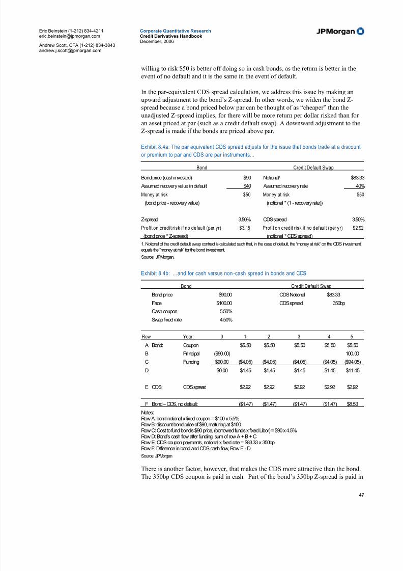
5/10/2018 JPM Credit Derivatives - slidepdf.com
http://slidepdf.com/reader/full/jpm-credit-derivatives-559e0102dc371 47/180
Eric Beinstein (1-212) [email protected]
Andrew Scott, CFA (1-212) [email protected]
Corporate Quantitative ResearchCredit Derivatives HandbookDecember, 2006
47
willing to risk $50 is better off doing so in cash bonds, as the return is better in the
event of no default and it is the same in the event of default.
In the par-equivalent CDS spread calculation, we address this issue by making an
upward adjustment to the bond’s Z-spread. In other words, we widen the bond Z-spread because a bond priced below par can be thought of as “cheaper” than the
unadjusted Z-spread implies, for there will be more return per dollar risked than for
an asset priced at par (such as a credit default swap). A downward adjustment to the
Z-spread is made if the bonds are priced above par.
Exhibit 8.4a: The par equivalent CDS spread adjusts for the issue that bonds trade at a discount
or premium to par and CDS are par instruments...
Bond Credit Default Swap
Bond price (cash invested) $90 Notional1 $83.33
Assumed recovery value in default $40 Assumed recovery rate 40%
Money at risk $50 Money at risk $50
(bond price - recovery value) (notional * (1 - recovery rate))
Z-spread 3.50% CDS spread 3.50%
Profit on credit risk if no default (per yr) $3.15 Profit on credit risk if no default (per yr) $2.92
(bond price * Z-spread) (notional * CDS spread)
1. Notional of the credit default swap contract is calculated such that, in the case of default, the “money at risk” on the CDS investment
equals the “money at risk” for the bond investment.
Source: JPMorgan.
Exhibit 8.4b: …and for cash versus non-cash spread in bonds and CDS
Bond Credit Default Swap
Bond price $90.00 CDS Notional $83.33Face $100.00 CDS spread 350bp
Cash coupon 5.50%
Swap fixed rate 4.50%
Row Year: 0 1 2 3 4 5
A Bond: Coupon $5.50 $5.50 $5.50 $5.50 $5.50
B Principal ($90.00) 100.00
C Funding $90.00 ($4.05) ($4.05) ($4.05) ($4.05) ($94.05)
D $0.00 $1.45 $1.45 $1.45 $1.45 $11.45
E CDS: CDS spread $2.92 $2.92 $2.92 $2.92 $2.92
F Bond – CDS, no default: ($1.47) ($1.47) ($1.47) ($1.47) $8.53
Notes:Row A: bond notional x fixed coupon = $100 x 5.5%Row B: discount bond price of $90, maturing at $100Row C: Cost to fund bond's $90 price, (borrowed funds x fixed Libor) = $90 x 4.5%Row D: Bond’s cash flow after funding, sum of row A + B + CRow E: CDS coupon payments, notional x fixed rate = $83.33 x 350bpRow F: Difference in bond and CDS cash flow, Row E - D
Source: JPMorgan
There is another factor, however, that makes the CDS more attractive than the bond.
The 350bp CDS coupon is paid in cash. Part of the bond’s 350bp Z-spread is paid in
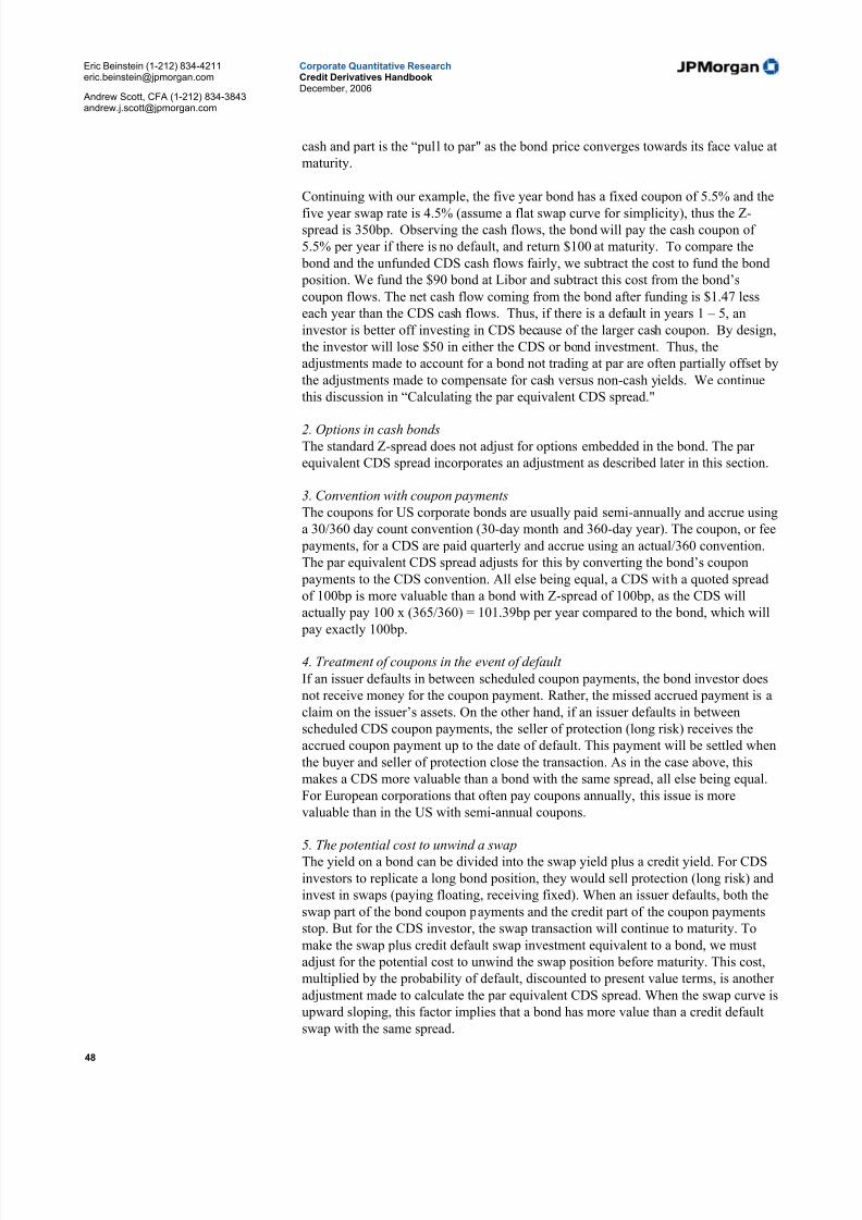
5/10/2018 JPM Credit Derivatives - slidepdf.com
http://slidepdf.com/reader/full/jpm-credit-derivatives-559e0102dc371 48/180
Eric Beinstein (1-212) [email protected]
Andrew Scott, CFA (1-212) [email protected]
Corporate Quantitative ResearchCredit Derivatives HandbookDecember, 2006
48
cash and part is the “pull to par" as the bond price converges towards its face value at
maturity.
Continuing with our example, the five year bond has a fixed coupon of 5.5% and the
five year swap rate is 4.5% (assume a flat swap curve for simplicity), thus the Z-spread is 350bp. Observing the cash flows, the bond will pay the cash coupon of
5.5% per year if there is no default, and return $100 at maturity. To compare the
bond and the unfunded CDS cash flows fairly, we subtract the cost to fund the bond
position. We fund the $90 bond at Libor and subtract this cost from the bond’s
coupon flows. The net cash flow coming from the bond after funding is $1.47 less
each year than the CDS cash flows. Thus, if there is a default in years 1 – 5, an
investor is better off investing in CDS because of the larger cash coupon. By design,
the investor will lose $50 in either the CDS or bond investment. Thus, the
adjustments made to account for a bond not trading at par are often partially offset by
the adjustments made to compensate for cash versus non-cash yields. We continue
this discussion in “Calculating the par equivalent CDS spread."
2. Options in cash bonds
The standard Z-spread does not adjust for options embedded in the bond. The par
equivalent CDS spread incorporates an adjustment as described later in this section.
3. Convention with coupon payments
The coupons for US corporate bonds are usually paid semi-annually and accrue using
a 30/360 day count convention (30-day month and 360-day year). The coupon, or fee
payments, for a CDS are paid quarterly and accrue using an actual/360 convention.
The par equivalent CDS spread adjusts for this by converting the bond’s coupon
payments to the CDS convention. All else being equal, a CDS with a quoted spread
of 100bp is more valuable than a bond with Z-spread of 100bp, as the CDS will
actually pay 100 x (365/360) = 101.39bp per year compared to the bond, which will
pay exactly 100bp.
4. Treatment of coupons in the event of default
If an issuer defaults in between scheduled coupon payments, the bond investor does
not receive money for the coupon payment. Rather, the missed accrued payment is a
claim on the issuer’s assets. On the other hand, if an issuer defaults in between
scheduled CDS coupon payments, the seller of protection (long risk) receives the
accrued coupon payment up to the date of default. This payment will be settled when
the buyer and seller of protection close the transaction. As in the case above, this
makes a CDS more valuable than a bond with the same spread, all else being equal.
For European corporations that often pay coupons annually, this issue is more
valuable than in the US with semi-annual coupons.
5. The potential cost to unwind a swapThe yield on a bond can be divided into the swap yield plus a credit yield. For CDS
investors to replicate a long bond position, they would sell protection (long risk) and
invest in swaps (paying floating, receiving fixed). When an issuer defaults, both the
swap part of the bond coupon payments and the credit part of the coupon payments
stop. But for the CDS investor, the swap transaction will continue to maturity. To
make the swap plus credit default swap investment equivalent to a bond, we must
adjust for the potential cost to unwind the swap position before maturity. This cost,
multiplied by the probability of default, discounted to present value terms, is another
adjustment made to calculate the par equivalent CDS spread. When the swap curve is
upward sloping, this factor implies that a bond has more value than a credit default
swap with the same spread.

5/10/2018 JPM Credit Derivatives - slidepdf.com
http://slidepdf.com/reader/full/jpm-credit-derivatives-559e0102dc371 49/180
Eric Beinstein (1-212) [email protected]
Andrew Scott, CFA (1-212) [email protected]
Corporate Quantitative ResearchCredit Derivatives HandbookDecember, 2006
49
Calculating the par-equivalent CDS spread
The par equivalent CDS spread is calculated using an iterative process. Each iteration
consists of the following two steps.
1. For a given par equivalent CDS spread and assumed recovery rate, we
calculate a curve of default probabilities. The actual calculation involves
numeric integration (using the same model that underlies the CDSW
calculation on Bloomberg), however a useful approximation is: Probability
of default = CDS Spread / (1 – Recovery)
2. We use the risk-free curve and the default probabilities found in step 1 to
calculate the value of the bond
We repeat these steps until the bond price found in step 2 matches the market price.
Note that a par equivalent CDS spread calculator is available on the Credit
Derivatives homepage found in www.morganmarkets.com.
We return to our five year, 5.5% coupon $90 bond, introduced in Exhibit 8.4, to
illustrate how we calculate the par equivalent CDS spread.
We start with an initial guess of the par equivalent CDS spread and, along with a
recovery assumption, use it to calculate a curve of default probabilities. Suppose we
guess that a bond’s par equivalent CDS spread is 341bp (a rather educated guess) and
assume its recovery rate is 40%. This implies an annual default probability of
approximately 5.7% = 3.41%/(1-40%). (We do not use this approximation in our
model, however, but use the same calculation as in the CDSW calculator).
We calculate the value of the bond using the default probabilities, risk-free discount
factors from the Libor/Swap curve, and the recovery rate assumption. We value the
bond by separating the bond into two payment streams: 1) the coupon payments, and
2) the principal payment, and value each stream under the default and no defaultscenarios. The value of the payment streams are summed to find the value of the
bond.
In the scenario where the company survives, we receive the coupon and principal
payments (Exhibit 8.5, row F). We find the risky present value of the cash flows by
multiplying them by the discount factor (row A) and the probability of survival (row
B). In other words, this is the present value of the bond’s cash flows discounted by
the likelihood of the cash flows being paid. The sum of the flows is $81.47.
In the scenario where the company defaults, the coupon payments stop and we are
left with a bond that is worth $40, as per our assumptions. We assume that the
default can happen at the end of the year, immediately before a coupon payment. As
a default can happen only once, we discount $40 not by the cumulative probability of default, but by the probability of default in a particular year. This conditional
probability of default can be calculated by subtracting the cumulative probabilities of
survival in adjacent years (refer to Section 4 for more discussion on probabilities).
The expected value of the bond in the default scenario is $8.53 (row J).
The sum of the two scenarios is $90, the price of the bond. Thus, a CDS spread of
341bp produces a probability curve that makes the expected value of the bond’s cash
flow equal to the price of the bond. If we had not guessed this spread initially, we
would iterate until the $90 expected cash flow was calculated. In our simplified
example, 341bp is the par equivalent CDS spread.

5/10/2018 JPM Credit Derivatives - slidepdf.com
http://slidepdf.com/reader/full/jpm-credit-derivatives-559e0102dc371 50/180
Eric Beinstein (1-212) [email protected]
Andrew Scott, CFA (1-212) [email protected]
Corporate Quantitative ResearchCredit Derivatives HandbookDecember, 2006
50
Note that in our exact model, default can occur at any point in time and we assume
that the principal recovery is paid at the actual time of default. Additionally, we
adjust for the factors described in Exhibit 8.3.
Exhibit 8.5: A bond’s p ar-equivalent CDS spread makes the expected value of the cash flow s equal to the curr ent market price.
Bond Credit Default Swap
Bond price $90.00 CDS Notional $83.33
Face $100.00 CDS spread 341 bp
Cash coupon 5.5% Recovery rate 40%
Swap fixed rate 4.5% Clean spread 5.7%= (341 / (1-40%)
Row Year: 0 1 2 3 4 5
A Discount factors 0.96 0.92 0.88 0.84 0.80
B Probability of survival 94.6% 89.5% 84.7% 80.2% 75.8%
C Probability of default 5.4% 5.1% 4.8% 4.6% 4.3%
Scenario 1: no default
D Coupon $5.50 $5.50 $5.50 $5.50 $5.50
E Principal $100.00
F $5.50 $5.50 $5.50 $5.50 $105.50
G Probability weighted PV, no default $4.98 $4.51 $4.08 $3.70 $64.21 $81.48
Scenario 2: default
H Value of bond principal $40.00 $40.00 $40.00 $40.00 $40.00
J Probability weighted PV, default $2.06 $1.86 $1.69 $1.53 $1.38 $8.53
K $90.00
Notes:Row A: Discount factors based on the flat swap curve, = 1 / (1+4.5%) ̂ t
Row B: Probability of survival approximation based on the clean spread = 1 / (1+5.7%)̂ t. See Section 4 for more information.
Row C: Probability of default = 1 – probability of survival in year 1, and the difference between cumulative probabilities of survival in years 2-5
Row D: Bond’s coupon
Row E: Bond’s principal payment of $100 at maturity
Row F: Row D + E
Row G: Risky present value of scenario 1 = (row F) x (row A) x (row B)
Row H: Recovery value of bond after default
Row J: Risky present value of scenario 2 = (row H) x (row A) x (Row C)
Row K: Sum of risky PV of scenario 1 and 2 = expected present value of bond’s cash flows
Source: JPMorgan.
We can also consider our bond and the funded component described in Exhibit 8.4b
and apply the same methodologies. Assume we have a long bond and short risk CDS
position. Recall we have sized the CDS position so the bond and CDS both have $50
at risk. We analyze the cash flows in two scenarios, if the bond survives or if it
defaults, and use the probabilities calculated from the CDS spread to evaluate the
scenarios.

5/10/2018 JPM Credit Derivatives - slidepdf.com
http://slidepdf.com/reader/full/jpm-credit-derivatives-559e0102dc371 51/180
Eric Beinstein (1-212) [email protected]
Andrew Scott, CFA (1-212) [email protected]
Corporate Quantitative ResearchCredit Derivatives HandbookDecember, 2006
51
Exhibit 8.6: In our simpl ified example, a CDS spread of 341bp is equi valent to a Z-spread of 350bp adjusted for t he discou nt bond
Bond Credit Default Swap
Bond price $90.00 CDS Notional $83.33
Face $100.00 CDS spread 341 bpCash coupon 5.50% Recovery Rate 40%
Z-spread 3.50% Clean spread 5.7%
Swap fixed rate 4.50%
Row Year: 0 1 2 3 4 5
A Bond: Coupon $5.50 $5.50 $5.50 $5.50 $5.50
B Principal ($90.00) 100.00
C Funding $90.00 ($4.05) ($4.05) ($4.05) ($4.05) ($94.05)
D $0.00 $1.45 $1.45 $1.45 $1.45 $11.45
E CDS: CDS spread $2.84 $2.84 $2.84 $2.84 $2.84
F Bond - CDS, no default: ($1.39) ($1.39) ($1.39) ($1.39) $8.61
Scenario 1: No default
G Discount factors 0.96 0.92 0.88 0.84 0.80
H Probability of survival 94.6% 89.5% 84.7% 80.2% 75.8% Sum of PV
J Present value, no default ($1.26) ($1.14) ($1.03) ($0.94) $5.24 $0.86
Scenario 2: Default
K CDS payment $50.00 $50.00 $50.00 $50.00 $50.00
L Value of bond principal $40.00 $40.00 $40.00 $40.00 $40.00
MFunding payment, includingcoupon ($94.05) ($94.05) ($94.05) ($94.05) ($94.05)
N ($4.05) ($4.05) ($4.05) ($4.05) ($4.05)
O Probability of default 5.4% 5.1% 4.8% 4.6% 4.3% Sum of PV
P Present value, default ($0.21) ($0.19) ($0.17) ($0.15) ($0.14) ($0.86)
Q $0.00
Row A - F: Refer to exhibit 8.4b
Row G - Discount factors based on the flat swap curve, = 1 / (1+4.5) ̂ t
Row H: Probability of survival approximation based on the clean spread = 1 / (1+5.7%)̂ t. See Section 4 for more information.
Row J: Risky present value of scenario 1 = (row F) x (row G) x (row H)
Row K: CDS payment in default = (1 – RR) x notional
Row L: Recovery value of bond after default
Row M: Unwind value of the funding = borrowed money + accrued interest paid in final year
Row N: Row K + L + MRow O: Risky Probability of default = 1 – probability of survival in year 1, and the difference between probabilities of survival in years 2-5
Row P: Risky present value of scenario 2 = (row N) x (row G) x (Row O)
Row Q: Sum of risky PV of scenario 1 and 2 = expected present value of bond + funding + CDS cash flows
Source: JPMorgan.
If the bond survives, we will realize the cash flows in row F. The risky present value
of these cash flows is $0.86.
If the company defaults (again, we assume default on the last day of the year), the
CDS position will receive (1- recovery) x notional, or (1-40%) x (83.33) = $50. The
value of our long bond position is $40, by assumption. Furthermore, we must pay
back our funding principal amount, plus accrued interest for the year. If there is a

5/10/2018 JPM Credit Derivatives - slidepdf.com
http://slidepdf.com/reader/full/jpm-credit-derivatives-559e0102dc371 52/180
Eric Beinstein (1-212) [email protected]
Andrew Scott, CFA (1-212) [email protected]
Corporate Quantitative ResearchCredit Derivatives HandbookDecember, 2006
52
default, we will lose $4.05 in any one year, given our assumptions. The risky present
value our position in this scenario is -$0.86 (row J).
The value of our two scenarios is +$0.86 - $0.86 = $0. Again, a CDS spread of
341bp provides a probability curve that makes the expected value of our cash flowszero, analogous to a fairly priced swap, or a par security.
Methodology for isolating credit risk in bonds withembedded options
Many high-yield bonds have embedded options, usually call options. A call optiongives the issuer the right, but not the obligation, to buy the bond back from the holder at a predetermined price at a future date. Often there is more than one call date and call price in a single bond. The call schedule of a typical bond is shown in Exhibit 8.7.
Our valuation framework is to observe a bond’s market price and calculate a spread(the par equivalent CDS spread) that reflects the credit risk of the bond. Difficulties
arise because we must separate the value of the embedded option from the market price of the bond.
For example, suppose an issuer has the following two bonds outstanding:
A. A standard bullet bond (no embedded option) with an 8% coupon and 1-Jun-2010 maturity.
B. A callable bond with an 8% coupon and 1-Jun-2010 maturity. The bond iscallable on 1-Jun-2008.
If bond B did not have the embedded call option, the two bonds would be identical.Suppose the market price of bond A is $110 and the market price of bond B is $103.
In this case, we could precisely determine the value of the option at $110 - $103 =$7.
Consider a different issuer that has a standard bullet bond outstanding with a 9%coupon and 1-Nov-2013 maturity. Assume the market price of the bond is $102.Suppose the issuer wants to issue another 9% 1-Nov-2013 bond—with the twist thatthis new bond is callable on 1-Nov-2008 at a price of $102. What is the value of thisnew bond? The new bond should be worth less than $102 (the price of the non-callable bond), but how much less? The value of the new bond depends on the valueof the embedded call option. Suppose a dealer was willing to quote a 1-Nov-2008$102 strike call option on the old bond at a price of $3. In this case, an investor couldreplicate the risk in the new bond by buying the old bond and selling the call option.We would therefore estimate the value of the new bond to be no less than $102 - $3= $99. Where does the $3 value of the come from? The value of this option dependson the volatility of the underlying, i.e., it depends on the volatility of the old bond.
Now suppose the new bond is issued and a year later the older bond becomes illiquidwith no observable market price. Suppose the callable bond is now being quoted at$101. We want to calculate a par equivalent CDS spread for the bond based on thismarket quote. To do so we need to estimate the value of the option and we need a bond option valuation model.
We think of the value of the callable bond as consisting of two parts:
Value of Callable Bond = Value of Underlying Non-Callable Bond – Value of Call Option
Call Date Call Price
07/15/2007 104.250
07/15/2008 102.125
07/25/2009 100.000The company has the right to buy the bond at a
price of $104.25 from 7/15/2007 – 7/14/2008. It
then has the right to buy the bond at $102.125 from
7/15/2008 – 7/25/2009. 7/25/2009 is the maturity
date of the bond.
Source: JPMorgan
Exhibit 8.7: Example of typical callschedule

5/10/2018 JPM Credit Derivatives - slidepdf.com
http://slidepdf.com/reader/full/jpm-credit-derivatives-559e0102dc371 53/180
Eric Beinstein (1-212) [email protected]
Andrew Scott, CFA (1-212) [email protected]
Corporate Quantitative ResearchCredit Derivatives HandbookDecember, 2006
53
The underlying non-callable bond is the bond stripped of the embedded option.
The par equivalent CDS spread for a callable bond is found by the same iterative process that we use for a non-callable bond. For a given guess at the par equivalent
CDS spread, we use a model to value the callable bond. We adjust the guess until our model value of the callable bond is equal to the price quoted in the market.
To value the call option, we use a separate model set up to value options on credit-risky bonds. This approach to the option valuation assumes that the issuer calls the bond when it is economically rational, without taking into account the issuer’sfinance costs. In reality, there may be significant costs for an issuer when calling a bond, especially if the issuer must issue a new bond to finance the call. For thisreason, an issuer may postpone a call to a later date or not call the bond at all. If our model is otherwise correct, our approach is more likely to overestimate the value of the option. For a given par equivalent CDS spread, this may lead us to underestimatethe value of the callable bond, which will lead us to solve for a par equivalent CDSspread that is too low.
How does our option valuation model work?The value of the option is determined primarily by the value and volatility of theunderlying. When choosing an option valuation model we are also choosing how tospecify the volatility of the underlying. Our methodology is based on the observationthat the value of the underlying is driven by changes in
• the term structure of default-free interest rates, and
• the credit risk of the issuer.
In our model, we use the Libor/swap rates as the default-free interest rates and the par equivalent CDS spread of the bond as the measure of credit risk.
Prices of interest rate swaptions provide market information about volatility in theLibor/swap curve. Our model is calibrated to fit the prices of swaptions where theswap matures on the same date as the bond. For most bonds, especially in less creditrisky bonds, the volatility in interest rates is the most important determinant of thevolatility of the value of the bond. The less credit-risky bonds are also the bonds withthe most valuable call option and, thus, the bonds for which it is most important thatwe value the option correctly. Indeed, the call option in the most credit-risky bonds isusually far out of the money since such bonds are priced significantly below par andthe call prices are usually above par.
We must also specify the volatility of the bond’s par equivalent CDS spread and thecorrelation between interest rates and the spread. While it can be argued that for
some issuers the correlation should be negative and for others it should be positive,we find it most reasonable to set the correlation to zero for all bonds. Finally, spreadvolatility can be estimated by the historical volatility of historical CDS spreads for the bond’s issuer. In our High Yield Spread Curve Report, we calculate the par equivalent CDS spread for three different spread volatilities to show the sensitivities.We also report six-month historical spread volatility in order to see how our assumption on future volatility fits the recently observed credit volatility.
How does the par equivalent CDS spread differ from a standard OAS?For an investment grade bond, an embedded option is often dealt with by calculatingan OAS (option adjusted spread) instead of the Z-spread. On Bloomberg this can bedone using the OAS1 calculator. An OAS is directly comparable to a Z-spread and

5/10/2018 JPM Credit Derivatives - slidepdf.com
http://slidepdf.com/reader/full/jpm-credit-derivatives-559e0102dc371 54/180
Eric Beinstein (1-212) [email protected]
Andrew Scott, CFA (1-212) [email protected]
Corporate Quantitative ResearchCredit Derivatives HandbookDecember, 2006
54
has the same drawbacks compared to the par equivalent CDS spread (see previoussection).
The par equivalent CDS spread is not directly comparable to a standard OAS as its
volatility assumptions are different. The bond price volatility implicit in the par equivalent CDS spread calculation is determined by: 1) the interest rate volatility, 2)the spread volatility, 3) the correlation between interest rate and spread, and 4) the probability of jump to default. In comparison, the standard OAS calculation ignoresthe jump to default and collects the interest rate, spread, and correlation into a singlevolatility input that can be loosely thought of as the volatility of the issuer’s yieldcurve. The par equivalent CDS spread calculation is most comparable to the OAScalculation when the interest rate and spread volatility are the same and thecorrelation between the two is one. However, even in this special case, the par equivalent CDS spread is different because it specifically takes into account the risk of default.
A brief note on the technical details
The term structure model we use in our option valuation methodology is a standardone-factor model for the instantaneous spot rate with time-dependent volatility andmean reversion. The distribution of the spot rate is set to lognormal and the meanversion to 0.05.
The model’s second factor is the hazard rate, or the default intensity, which weassume is lognormally distributed without mean reversion and with constantvolatility. The hazard rate volatility is set equal to the number that is labeled “SpreadVol” in the US bond versus CDS daily analytic reports. The recovery rate is fixedand constant for all bonds of the same issuer.

5/10/2018 JPM Credit Derivatives - slidepdf.com
http://slidepdf.com/reader/full/jpm-credit-derivatives-559e0102dc371 55/180
Eric Beinstein (1-212) [email protected]
Andrew Scott, CFA (1-212) [email protected]
Corporate Quantitative ResearchCredit Derivatives HandbookDecember, 2006
55
9. Basis Trading
Understanding the difference between bonds and creditdefault swap spreads
Basis refers to the difference, in basis points, between a credit default swap spreadand a bond’s par equivalent CDS spread with the same maturity dates. Basis is either zero, positive, or negative.
Negative basisIf the basis is negative, then the credit default swap spread is lower (tighter) than the bond’s spread. This occurs when there is excess protection selling (investors lookingto go long risk and receive periodic payments), reducing the CDS spread.
Structured credit activity: Excess protection selling may come from structured creditissuers, for example, who sell protection in order to fund coupon payments to the
buyers of structured credit products.
Borrowing costs: Protection selling may also come from investors who lend or borrow at rates above Libor. For these investors, it may be more economical to sell protection (long risk) and invest at spreads above Libor, rather than borrow moneyand purchase a bond.
Risk of non-deliverables: In cases of restructuring associated with M&A activity, bonds may sometimes be transferred to a different entity, which may leave the CDScontract without any deliverable bonds (i.e., without a Succession event, described inPart I). In cases such as this (or where investors feel there is a risk of this event),CDS will tighten, often leading to a negative basis.
Bond new issuance: When bond issuance increases, the laws of supply and demanddictate that prices must drop, forcing credit spreads higher. This usually widens bondspreads more than CDS spreads.
An investor could buy the bond (long risk), then buy protection (short risk), tocapture this pricing discrepancy. In this trade, an investor is not exposed to defaultrisk, yet still receives a spread. This is, therefore, a potential arbitrage opportunity12.Trading desks at investment banks and other investors who can fund long bond positions cheaply (borrowing at or near Libor) will typically enter into this positionwhen the negative basis exceeds 10–25bp.
12The trade does have mark-to-market and counterparty risk and may have a gain or loss in
default as the cash flows received on the two legs of the trade prior to default may differ.
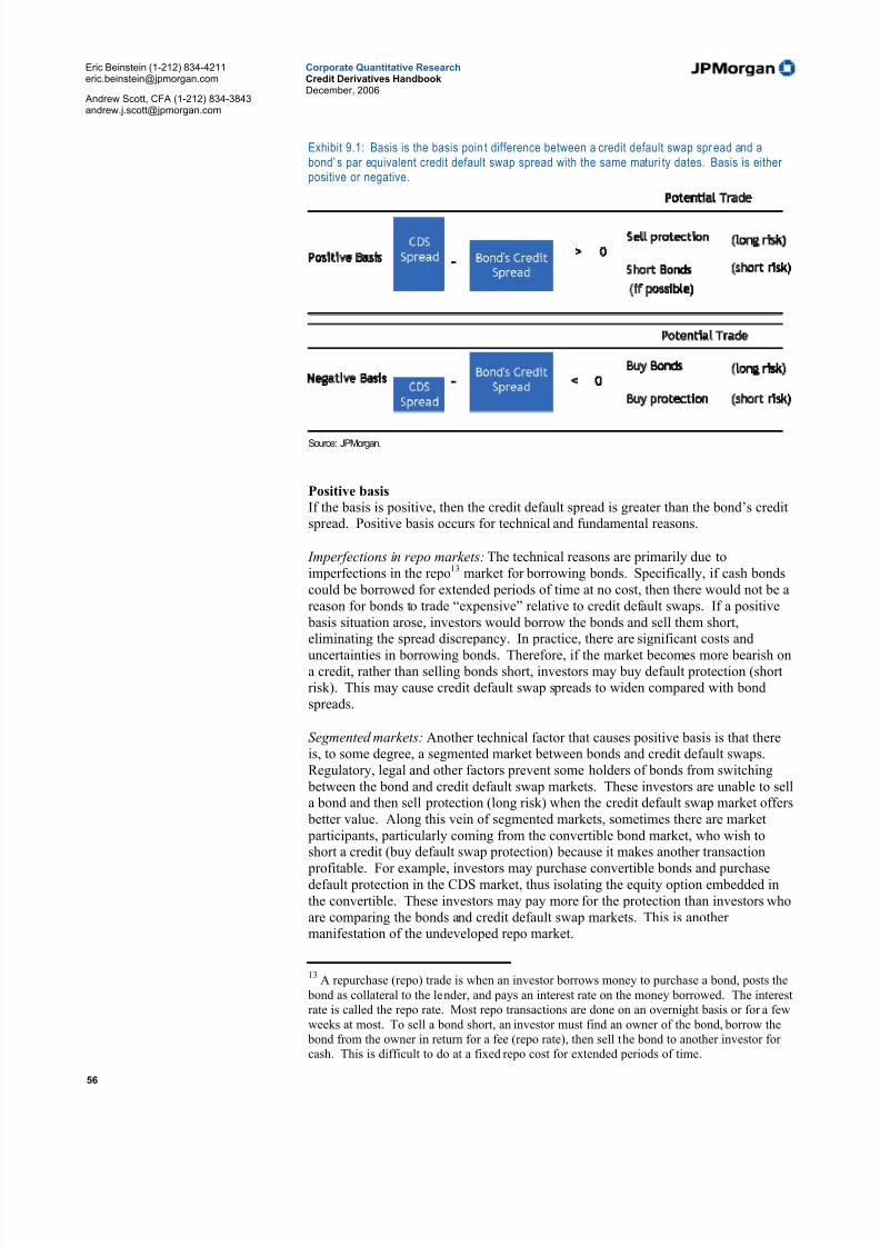
5/10/2018 JPM Credit Derivatives - slidepdf.com
http://slidepdf.com/reader/full/jpm-credit-derivatives-559e0102dc371 56/180
Eric Beinstein (1-212) [email protected]
Andrew Scott, CFA (1-212) [email protected]
Corporate Quantitative ResearchCredit Derivatives HandbookDecember, 2006
56
Exhibit 9.1: Basis is the basis poin t difference between a credit default swap spr ead and abond’ s par equivalent credit default swap spread with the same maturi ty dates. Basis is either positive or negative.
Source: JPMorgan.
Positive basisIf the basis is positive, then the credit default spread is greater than the bond’s creditspread. Positive basis occurs for technical and fundamental reasons.
Imperfections in repo markets: The technical reasons are primarily due toimperfections in the repo13 market for borrowing bonds. Specifically, if cash bondscould be borrowed for extended periods of time at no cost, then there would not be areason for bonds to trade “expensive” relative to credit default swaps. If a positive basis situation arose, investors would borrow the bonds and sell them short,eliminating the spread discrepancy. In practice, there are significant costs anduncertainties in borrowing bonds. Therefore, if the market becomes more bearish ona credit, rather than selling bonds short, investors may buy default protection (shortrisk). This may cause credit default swap spreads to widen compared with bondspreads.
Segmented markets: Another technical factor that causes positive basis is that thereis, to some degree, a segmented market between bonds and credit default swaps.Regulatory, legal and other factors prevent some holders of bonds from switching between the bond and credit default swap markets. These investors are unable to sella bond and then sell protection (long risk) when the credit default swap market offers better value. Along this vein of segmented markets, sometimes there are market participants, particularly coming from the convertible bond market, who wish toshort a credit (buy default swap protection) because it makes another transaction
profitable. For example, investors may purchase convertible bonds and purchasedefault protection in the CDS market, thus isolating the equity option embedded inthe convertible. These investors may pay more for the protection than investors whoare comparing the bonds and credit default swap markets. This is another manifestation of the undeveloped repo market.
13A repurchase (repo) trade is when an investor borrows money to purchase a bond, posts the
bond as collateral to the lender, and pays an interest rate on the money borrowed. The interestrate is called the repo rate. Most repo transactions are done on an overnight basis or for a fewweeks at most. To sell a bond short, an investor must find an owner of the bond, borrow the
bond from the owner in return for a fee (repo rate), then sell the bond to another investor for cash. This is difficult to do at a fixed repo cost for extended periods of time.

5/10/2018 JPM Credit Derivatives - slidepdf.com
http://slidepdf.com/reader/full/jpm-credit-derivatives-559e0102dc371 57/180
Eric Beinstein (1-212) [email protected]
Andrew Scott, CFA (1-212) [email protected]
Corporate Quantitative ResearchCredit Derivatives HandbookDecember, 2006
57
Cheapest-to-deliver option: A fundamental factor that creates positive basis is thecheapest-to-deliver option. A long risk CDS position is short the cheapest-to-deliver option. If there is a credit event, the protection buyer (short risk) is contractuallyallowed to choose which bond to deliver in exchange for the notional amount. This
investor will generally deliver the cheapest bond in the market. When there is acredit event, bonds at the same level of the capital structure generally trade at or near the same price (except for potential differences in accrued interest) as they will betreated similarly in a restructuring. Still, there is the potential for price disparity.Thus, protection sellers (long risk) may expect to receive additional spread comparedto bonds for bearing this risk. This would lead to CDS spreads trading wider than bond spreads and therefore contribute to positive basis.
Bond covenants: In addition, bond holders have actual or potential rights that sellersof CDS protection do not have. These may include bonds being called with a changein control of the company. Also, bond holders may receive contingent payments if acompany wishes to change a term of a bond. Bond holders may benefit from a tender offer, or may be treated better in a succession event. These issues are difficult to
quantify but can cause bonds to perform significantly better than CDS in certaincircumstances.
Non-default credit events: Finally, a CDS contract may payout in a variety of events,such as restructuring, that are not actual defaults. The CDS premium will therefore be higher than the bond spread to account for this.
Trading the basis
Investors frequently seek to exploit discrepancies in the bond-CDS basis at a single-name level by trading basis packages. A positive basis package consists of a short position in the bond coupled with short CDS protection position. A negative basis package consists of a long bond position and a long CDS protection position. In bothcases, the principle is that the bond and CDS position offset each other in the case of
default, allowing the investor to take a view on the relative pricing of bonds and CDSwithout taking on credit risk. Basis trades are normally hedged against interest raterisk.
Trading a positive basis is more complex than a negative basis for two main reasons:
• rather than buying the bond outright, the investor must short the bond viareverse repo
• the CDS contract contains a degree of optionality in terms of deliverable bonds in default. Therefore, if the bond defaults, it is possible that the bonddelivered into the CDS contract would not match the investor’s short position.
Negative basis packages are easier to implement as it is easy to take a short risk position in CDS with the same maturity date of the bond. Exhibit 9.2 is a stylizedexample of a negative basis trade. A three year, 8% bond is trading at par.Assuming our investor funds the bond at a fixed rate of 5%, she will net 3%annually. She pays 280bp annually for CDS protection, thus nets $0.20 per year (column A+B+C), or $0.60 over three years. The present value of $0.60 is $0.55(assuming a flat Libor curve of 5%), and the risky present value is $0.51. Note thatwe are ignoring day count conventions, which would increase the cost of CDS protection given it is paid on the actual/360 convention. Furthermore, we are not bootstrapping the probability of default curve, but using a rough approximation(default probability = spread / (1-RR) = 0.028/(1-.04) = 4.67%. The two year default

5/10/2018 JPM Credit Derivatives - slidepdf.com
http://slidepdf.com/reader/full/jpm-credit-derivatives-559e0102dc371 58/180
Eric Beinstein (1-212) [email protected]
Andrew Scott, CFA (1-212) [email protected]
Corporate Quantitative ResearchCredit Derivatives HandbookDecember, 2006
58
adjustment is calculated 1 / (1+4.67%)2). Thus, we expect to earn $0.51 withoutexposure to credit risk. This methodology is the same as the par equivalent CDSspread calculation, discussed in Section 8.
Exhibit 9.3 is a stylized example of a negative basis trade with a discount bond. Thethree year 6.86% coupon bond is trading at $97, but as in Exhibit 9.2, has a yield tomaturity of 8%.
With a discount bond, our investor does not buy $100 of CDS protection. Rather,she buys enough protection to be neutral in default. Assuming a 40% recovery ratefor the bond, she expects to lose (initial bond price – recovery price) = $97 - $40 =$57 on the defaulted bond. Thus she buys $95 of CDS protection, as notional x (1-recovery rate) = payment in default, $95 x (1-40%) = $57.
She will lose $0.66 each year, before earning $3 as the $97 priced bond matures at par in year three. She nets $1.05, or $0.80 after discounting, or $0.61, after adjustingfor the probability of default.
Exhibit 9.2: Negative basis tr ade using a par bond.
Bond Price $100.00
Bond Coupon 8.00%
YTM = 8.00%
Swap Rate 5.00%
CDS spread 280bp
Bond (A) (B) (A)+(B) (C) A+B+C Discounted
payment Bond Funding Net bond CDS Net Cash at risk free Default
type Years cash flow at fixed Libor cash flow cost Flow rate (Libor) adjusted
Principal 0.0 -$100.00 $100.00 $0.00 $0.00 $0.00 $0.00 $0.00
0.5 $4.00 -$2.50 $1.50 -$1.40 $0.10 $0.10 $0.10
1.0 $4.00 -$2.50 $1.50 -$1.40 $0.10 $0.10 $0.09
Coupons 1.5 $4.00 -$2.50 $1.50 -$1.40 $0.10 $0.09 $0.09
2.0 $4.00 -$2.50 $1.50 -$1.40 $0.10 $0.09 $0.08
2.5 $4.00 -$2.50 $1.50 -$1.40 $0.10 $0.09 $0.08
3.0 $4.00 -$2.50 $1.50 -$1.40 $0.10 $0.09 $0.08
Principal 3.0 $100.00 -$100.00 $0.00 $0.00 $0.00 $0.00 $0.00
Total $9.00 -$8.40 $0.60 $0.55 $0.51
Source: JPMorgan.

5/10/2018 JPM Credit Derivatives - slidepdf.com
http://slidepdf.com/reader/full/jpm-credit-derivatives-559e0102dc371 59/180
Eric Beinstein (1-212) [email protected]
Andrew Scott, CFA (1-212) [email protected]
Corporate Quantitative ResearchCredit Derivatives HandbookDecember, 2006
59
Exhibit 9.2: Negative basis trade using a discount bond.
Bond Price $97.00 Default analysis
Bond Coupon 6.86% Recovery Rate 40%
YTM = 8.00% Bond's loss in default $57Swap Rate 5.00% CDS notional for equal loss $95
CDS Spread 280bp
Bond (A) (B) (A)+(B) (C) A+B+C Discounted
payment Bond Funding Net bond CDS Net Cash at risk free Default
type Years cash flow at fixed Libor cash flow cost Flow rate (Libor) adjusted
Principal 0.0 -$97.00 $97.00 $0.00 $0.00 $0.00 $0.00 $0.00
0.5 $3.43 -$2.43 $1.01 -$1.33 -$0.33 -$0.32 -$0.31
1.0 $3.43 -$2.43 $1.01 -$1.33 -$0.33 -$0.31 -$0.30
Coupons 1.5 $3.43 -$2.43 $1.01 -$1.33 -$0.33 -$0.30 -$0.28
2.0 $3.43 -$2.43 $1.01 -$1.33 -$0.33 -$0.29 -$0.27
2.5 $3.43 -$2.43 $1.01 -$1.33 -$0.33 -$0.29 -$0.263.0 $3.43 -$2.43 $1.01 -$1.33 -$0.33 -$0.28 -$0.25
Principal 3.0 $100.00 -$97.00 $3.00 $0.00 $3.00 $2.59 $2.27
Total $9.03 -$7.98 $1.05 $0.80 $0.61
Source: JPMorgan.
Logistics in default
A negative basis package is usually considered to be perfectly hedged in the case of default, but as the three separate components of the package (bond, swap/bondfunding and CDS) all behave differently, the behaviour of the package in default ismore complex. The effects of default on different parts of the package are as follows:
CDS contract and defaulted bond: The bond, by definition, is deliverable into theCDS contract (as the bond is issued by the reference entity). So, if a default were to
occur, we can deliver the bond into the CDS contract, and receive par (the price weinitially paid for the bond) in return.
Coupon payments: Bondholders are not entitled to any accrued coupon paymentson default. However, buyers of CDS protection must still pay any interest accrued upto the default date to the seller of protection. For bonds that pay coupons annually, inthe worst case scenario (the bond defaults the day before a coupon payment is due),an investor could lose a full year’s worth of accrued interest on the notional invested,while still paying for a full year of CDS protection.
Funding: The interest rate component of a bond must be hedged in the negative basis trade. There can be a cost of unwinding this hedge early, whether it wascreated using a fixed for floating swap, through funding the bond, or an asset swap.
An asset swap (detailed next), for example, does not knock out in the case of defaultof the associated bond meaning the investor is left with a residual swap position.Whether or not this position is in the favour of the investor depends on two factors:
• Movement of rates: If swap rates (and forward swap rates) are lower than predicted at the inception of the swap then the investor will be receiving payments of a lower value than they are making to the swap counterparty.Falling rates will result in a negative mark-to-market for the residual swap position in the case of default (all else equal).
• Dirty price of the bond: The bond is worth its dirty price at inception, butthe investor pays par for the (par) asset swap package. The value of the asset

5/10/2018 JPM Credit Derivatives - slidepdf.com
http://slidepdf.com/reader/full/jpm-credit-derivatives-559e0102dc371 60/180
Eric Beinstein (1-212) [email protected]
Andrew Scott, CFA (1-212) [email protected]
Corporate Quantitative ResearchCredit Derivatives HandbookDecember, 2006
60
swap at inception must be equivalent to the difference between par and the bond dirty price. If the bond was trading at a discount to par, this effect will be in the favor of the investor. The value will amortise over the life of theswap, as the price approaches par as the contract approaches maturity.
When using an asset swap, the behaviour in default outlined above implies that lower priced bonds with low coupons are the most attractive for negative basis trades, asthese are the least likely to cost the investor on default.
Asset Swap Spread
Commonly used in Europe, an asset swap is a way of trading a bond in which thefixed coupons on the bond are exchanged for floating payments that fluctuate in linewith Libor (or some other agreed rate). Essentially, this transforms the bond intosomething analogous to a floating rate note. In doing this, the investor is able tohedge out the interest rate risk inherent in owning a bond. The spread over Libor received on the floating side is called the asset swap spread, and can be considered to
give some measure of the bond's credit risk.
A par asset swap package consists of a bond and an asset swap, with the total package priced at par. It can be considered as a combination of three sets of cashflows: one from owning a bond, a set of fixed payments made to the swapcounterparty, and a set of floating payments received from the counterparty. Thesenet out into a single stream of payments resembling a floating-rate note priced at par.
Exhibit 9.3: The Asset Swap
Source: JPMorgan
Note that, as the asset swap package is priced at par, if the bond is trading away from par then the value of the swap must account for the difference. So if the bond istrading at a discount to par, the swap will initially be in the investors favour.Conversely, the swap will be against the investor if the bond is trading at a premium.Ignoring the effect of interest rates, the Mark-to-Market of the swap will graduallytrend toward zero as the difference between the dirty price and par amortises over thelife of the swap.
par
par
par
par
Libor + asset swap spread
coupon
coupon
dirtyprice
dirtyprice
swap
bond

5/10/2018 JPM Credit Derivatives - slidepdf.com
http://slidepdf.com/reader/full/jpm-credit-derivatives-559e0102dc371 61/180
Eric Beinstein (1-212) [email protected]
Andrew Scott, CFA (1-212) [email protected]
Corporate Quantitative ResearchCredit Derivatives HandbookDecember, 2006
61
Although the bond and swap are traded as a package, the swap does not knock out inthe case of default. This means that if the bond defaults, the investor will be exposedto interest rate risk, as well as any remaining MTM position resulting from the bondtrading away from par at inception.
Calculating the asset swap spreadThe asset swap spread can be computed using a simple equation of cashflowsargument on the swap portion of the package. As the package as a whole costs par,the purchaser must pay an additional par - dirty price to the swap counterparty atinception (or, equivalently, receive dirty price - par if the bond is at a premium). Theinvestor then pays the coupon and receives the asset swap spread over Libor for thelife of the swap. By equating the fixed and floating payment streams, we have:
( )∑ ∑ +=+−
i j
j ji DF a L DF c DP par
where: DP = dirty price of bond
c = bond coupona = Asset swap spread
L j = Libor rates DF i = risk-free discount factors.The asset swap spread is the value of a that solves this equation.
Notice that there are no risky discount factors involved in this calculation. This is because the swap does not knock out on default of the bond.

5/10/2018 JPM Credit Derivatives - slidepdf.com
http://slidepdf.com/reader/full/jpm-credit-derivatives-559e0102dc371 62/180
Eric Beinstein (1-212) [email protected]
Andrew Scott, CFA (1-212) [email protected]
Corporate Quantitative ResearchCredit Derivatives HandbookDecember, 2006
62
10. Trading Credit Curves
Curve trading in credit involves taking a view on the relative steepness of points on
the credit curve and trading the view that the curve will either steepen or flatten. For
example, an investor may believe that the curve of Company ABC will steepen over
time (10y - 5y spread will increase). To position for this an investor could sell
protection in the 5y point and buy protection in the 10y point. If the curve moves as
the investor predicts, as in Exhibit 10.1, then the investor will benefit. Trading the
curve as opposed to a single point can be useful where an investor is not sure which
point will move but has a view on the relative steepness of the curve. Additionally,
curve trading can mean an investor avoids an outright credit (default) exposure while
positioning for points in the curve moving (as opposed to trading a single point
where an investor must take outright default exposure).
Exhibit 10.1: Example Curve Trade for Company AB C
x-axis = Time in Years, y-axis = Spread, bp
0
20
40
60
80
100
120
140
160
180
0 1 2 3 4 5 6 7 8 9 10
Curve at Time, t=1
Curve at Time, t=2
10y-5y = 40bp
10y-5y = 48bp
Source: JPMorgan
Exhibit 10.2: iTraxx Curve Over Time
iTraxx Europe Main 10y - 5y Spread, bp
0
5
10
15
20
25
Jan-04 Apr-04 Jul-04 Oct-04 Jan-05 Apr-05 Jul-05 Oct-05 Jan-06
Source: JPMorgan
Credit curve movements can be significant and investors can look to position for
curve trades both on a company specific basis or on the market as a whole (see
Exhibit 10.2 the curve of iTraxx Europe Main over time).
Structuring curve trades involves trying to isolate the view on the curve. This makes
it important to understand the drivers of P+L on these trades so traders or investors
can assess whether their core view of curve steepening / flattening can be turned into
a profitable strategy. Understanding these drivers of P+L in curve trades should more
accurately allow for more profitable curve trading strategies. We structure this as
follows:
We first outline our framework for analyzing the P+L in curve trades.
We then apply this to common curve trades and highlight the common characteristics
of these.
Future notes in this series will examine Barbells and other curve themes.
Drivers of P+L in curve trades
A Framework For Analysing Curve Trades
When we look at trading credit curves there are four dimensions we need to look
across to analyse the expected profitability of any trading strategy:

5/10/2018 JPM Credit Derivatives - slidepdf.com
http://slidepdf.com/reader/full/jpm-credit-derivatives-559e0102dc371 63/180
Eric Beinstein (1-212) [email protected]
Andrew Scott, CFA (1-212) [email protected]
Corporate Quantitative ResearchCredit Derivatives HandbookDecember, 2006
63
Time: We need to understand how our curve trade will be affected by the passage of
time. This breaks down into the fee we earn, our 'Carry', and the way our position
moves along the credit curve over time, our ‘Slide’.
Sensitivity to spread changes: We need to understand how our trade will beaffected by parallel spread changes. As a first order effect we need to look at the P+L
sensitivity to spread movements (Duration effect), but we also need to understand the
second order P+L impact as our Durations change when spreads move giving us a
Convexity effect. There is also a third order effect which models the way our curve
shape changes as a function of our 5y point. Analysing the sensitivity to spread
changes at the trade horizon needs special care due to the Horizon Effect which
shows how our position changes over the horizon.
Default risk: We need to understand the trade’s exposure to underlying credit risk,
as our curve trade positions may leave us with default risk.
Breakevens and expected curve movements: Once we have understood all of the
other' risks to our curve trade, we need to put this together with our expectation
of curve moves and look at our ‘Breakeven’ levels. I.e. given the other risk factors that can affect the trade, how much of a curve move do we need for our
trade to breakeven over the horizon we are considering.
We tackle these dimensions in turn in this section and then turn to common curve
trading strategies to see how our framework for analysis can be applied to each
strategy to give more profitable trades.
• Time: Carry
The Carry of a curve trade is the income earned from holding the position over time.
For example, if we constructed a simple curve flattening trade buying protection on
$10mm notional for 5 years at 50bp and selling protection on $5mm notional for 10
years at 90bp (we will discuss trade structuring further on), we would end up with net
payments, or Carry, of -$5,000 over the first year as shown in Exhibit 10.314.
Exhibit 10.3: Carry Example
Buy Protection Sell Protection Total 1y CarryMaturity 5y 10yNotional ($) 10,000,000 5,000,000Spread 50bp 90bp1y Carry ($) -50,000 +45,000 -5,000
Source: JPMorgan
To generalize, the Carry on a curve trade is calculated as:
Carry Horizon = (Ntnl Leg1 × S Leg1 × Horizon) + (Ntnl Leg2 × S Leg2 × Horizon) [1]
Where,
NtnlLeg n : Notional of protection bought or sold on Leg n of the trade. This will be
positive if selling protection and negative if buying protection.
SLeg n : Annual Spread on leg n of the trade, expressed in % terms (Spread in bp /
10000).
Horizon: Length of time in which trade is being evaluated, in years.
14We usually look at Carry without any present value discounting.

5/10/2018 JPM Credit Derivatives - slidepdf.com
http://slidepdf.com/reader/full/jpm-credit-derivatives-559e0102dc371 64/180
Eric Beinstein (1-212) [email protected]
Andrew Scott, CFA (1-212) [email protected]
Corporate Quantitative ResearchCredit Derivatives HandbookDecember, 2006
64
• Time: Slide
Slide is the change in value of a position due to the passage of time, assuming that
our credit curve is unchanged . Intuitively, as we usually observe an upward sloping
credit curve (see Exhibit 10.4) as time passes we will ‘slide’ down the curve. So,
using the example in Exhibit 10.4, a 3y position slides down to become a 2y positionand a 5y position slides down to become a 4y position over a year horizon. If I had
sold protection in 5y and bought protection in 3y (a 3y/5y flattener), the 3y leg would
slide more than the 5y, as the 3y part of the curve is steeper than 5y in this example.
Exhibit 10.4: Slide Intuition
bp
0
20
40
60
80
100
0 1 2 3 4 5 6 7 8 9 10 Source: JPMorgan
At the end of this section we discuss two different ways to calculate Slide, depending
on what we assume is unchanged over time: i) hazard rates for each maturity tenor
(5y point), or ii) hazard rates for each calendar point (year 2010). In our analysis we
will use i) and keep hazard rates constant for each maturity tenor, which is theequivalent of keeping the spread curve constant (e.g. so that the 5y spread at 100bp
remains at 100bp) and sliding down these spreads due to time passing.
Horizon Effect
Slide also leads to another effect which we will call the Horizon Effect. The effect of
the change in Spreads and lessening of maturities over the horizon both imply a
change in Risky Annuities, which we call the Horizon Effect. This will have the
impact of changing the Duration-Weighting of trade over time, meaning the trade
essentially gets longer or shorter risk over the horizon. This can have a significant
impact when we look at sensitivity analysis at the horizon. We discuss these issues
later in this section.
Slide and Flat ForwardsThe way we model our hazard rates and Forward curves also affects how we
calculate Slide. As we have seen in Trading Credit Curves I , we model the Forward
curve as a Flat Forward curve. This means that the Forward spread (and hazard rates)
are taken as constant between points on the curve where spreads change. In terms of
our Slide, this could mean that we have no Slide over a given one month horizon if
we are on a flat part of the curve and larger Slide over a given one month horizon if
we are on a part of the curve where there is a step down. In order to account for this
we tend to have a method of interpolating between our step points, so that this is not
just a 'jump’ down. The method of interpolation may lead to some of the Slide
calculations requiring a little thought as they can be as much to do with the way we
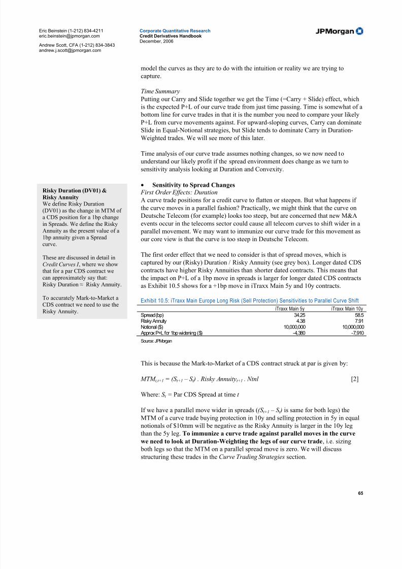
5/10/2018 JPM Credit Derivatives - slidepdf.com
http://slidepdf.com/reader/full/jpm-credit-derivatives-559e0102dc371 65/180
Eric Beinstein (1-212) [email protected]
Andrew Scott, CFA (1-212) [email protected]
Corporate Quantitative ResearchCredit Derivatives HandbookDecember, 2006
65
model the curves as they are to do with the intuition or reality we are trying to
capture.
Time Summary
Putting our Carry and Slide together we get the Time (=Carry + Slide) effect, whichis the expected P+L of our curve trade from just time passing. Time is somewhat of a
bottom line for curve trades in that it is the number you need to compare your likely
P+L from curve movements against. For upward-sloping curves, Carry can dominate
Slide in Equal-Notional strategies, but Slide tends to dominate Carry in Duration-
Weighted trades. We will see more of this later.
Time analysis of our curve trade assumes nothing changes, so we now need to
understand our likely profit if the spread environment does change as we turn to
sensitivity analysis looking at Duration and Convexity.
• Sensitivity to Spread Changes
First Order Effects: Duration
A curve trade positions for a credit curve to flatten or steepen. But what happens if
the curve moves in a parallel fashion? Practically, we might think that the curve on
Deutsche Telecom (for example) looks too steep, but are concerned that new M&A
events occur in the telecoms sector could cause all telecom curves to shift wider in a
parallel movement. We may want to immunize our curve trade for this movement as
our core view is that the curve is too steep in Deutsche Telecom.
The first order effect that we need to consider is that of spread moves, which is
captured by our (Risky) Duration / Risky Annuity (see grey box). Longer dated CDS
contracts have higher Risky Annuities than shorter dated contracts. This means that
the impact on P+L of a 1bp move in spreads is larger for longer dated CDS contracts
as Exhibit 10.5 shows for a +1bp move in iTraxx Main 5y and 10y contracts.
Exhibit 10.5: iTraxx Main Europe Long Risk (Sell Protection) Sensitivities to Parallel Curve Shift
iTraxx Main 5y iTraxx Main 10ySpread (bp) 34.25 58.5Risky Annuity 4.38 7.91Notional ($) 10,000,000 10,000,000Approx P+L for 1bp widening ($) -4,380 -7,910
Source: JPMorgan
This is because the Mark-to-Market of a CDS contract struck at par is given by:
MTM t,t+1 = (S t+1 – S t ) . Risky Annuityt+1 . Ntnl [2]
Where: S t = Par CDS Spread at time t
If we have a parallel move wider in spreads ((S t+1 – S t ) is same for both legs) the
MTM of a curve trade buying protection in 10y and selling protection in 5y in equal
notionals of $10mm will be negative as the Risky Annuity is larger in the 10y leg
than the 5y leg. To immunize a curve trade against parallel moves in the curve
we need to look at Duration-Weighting the legs of our curve trade, i.e. sizing
both legs so that the MTM on a parallel spread move is zero. We will discuss
structuring these trades in the Curve Trading Strategies section.
Risky Duration (DV01) &
Risky AnnuityWe define Risky Duration(DV01) as the change in MTM of a CDS position for a 1bp changein Spreads. We define the RiskyAnnuity as the present value of a1bp annuity given a Spreadcurve.
These are discussed in detail inCredit Curves I , where we showthat for a par CDS contract wecan approximately say that:Risky Duration ≈ Risky Annuity.
To accurately Mark-to-Market aCDS contract we need to use theRisky Annuity.

5/10/2018 JPM Credit Derivatives - slidepdf.com
http://slidepdf.com/reader/full/jpm-credit-derivatives-559e0102dc371 66/180
Eric Beinstein (1-212) [email protected]
Andrew Scott, CFA (1-212) [email protected]
Corporate Quantitative ResearchCredit Derivatives HandbookDecember, 2006
66
Duration analysis is intended to immunize our curve trade for market spread moves.
However, looking at this first order Duration effects is not the full story and we need
to consider second order effects by looking at Convexity.
Second Order Effects: ConvexityWe define Convexity as the change in MTM of a curve trade coming from changes
in Risky Annuity due to spreads moving. It measures the second order effect of how
our curve trade is affected due to Durations (or Risky Annuities) changing when
spreads change.
Why is there convexity in CDS positions?
We have seen that the Mark-to-Market of a CDS contract (in Equation [2]) is the
Change in Spread × The Risky Annuity, and:
∑=
∆≈
n
i
iii DF Psty RiskyAnnui
1
...1 [3]
Where , Psi ,is the Survival Probability to period i.15
DF i is the risk-free discount factor for period i
∆i is the length of period i
n is the number of periods.
If the spread curve parallel shifts (widens) by 100bp, this means that credit risk has
risen and survival probabilities have fallen. For a given spread widening, survival
probabilities decrease more for longer time periods as the impact of higher hazard
rates is compounded. This is illustrated in Exhibit 10.6 and Exhibit 10.7 where we
can see that the Probability of Survival decreases proportionately more at longer
maturities for a 100bp spread change.
Exhibit 10.6: Parallel Shift in Par Spread Curve
x-axis: Maturity Date; y-axis: Spread, bp
0
50
100
150
200
250
300
Feb-
06
Feb-
07
Feb-
08
Feb-
09
Feb-
10
Feb-
11
Feb-
12
Feb-
13
Feb-
14
Feb-
15
Feb-
16
Spreads at t
Spreads at t+1
Source: JPMorgan
Exhibit 10.7: Survival Probabilit ies for Parallel Shift in Spreads
x-axis: Maturity Date; y-axis: Survival probability, %
20%
30%
40%
50%
60%
70%
80%
90%
100%
Feb-06
Feb-07
Feb-08
Feb-09
Feb-10
Feb-11
Feb-12
Feb-13
Feb-14
Feb-15
Feb-16
Survival Probabilities at t
Survival Probabilities at t+1
Source: JPMorgan
Looking at Equation [3], we can see this has the effect of making our Risky
Annuities decrease more for longer maturity CDS contracts as Exhibit 10.8
illustrates.
15See Trading Credit Curves I for a more complete explanation of Survival Probabilities and
Risky Annuities.

5/10/2018 JPM Credit Derivatives - slidepdf.com
http://slidepdf.com/reader/full/jpm-credit-derivatives-559e0102dc371 67/180
Eric Beinstein (1-212) [email protected]
Andrew Scott, CFA (1-212) [email protected]
Corporate Quantitative ResearchCredit Derivatives HandbookDecember, 2006
67
Spreads Risky Annuit ies
Spreads Risky Annuit ies
Exhibit 10.8: Risky Annuit y Changes for Parallel Shift in Spreads
x-axis: Maturity Date; y-axis: Duration
0.00
1.00
2.00
3.00
4.00
5.00
6.00
7.00
Feb-
06
Feb-
07
Feb-
08
Feb-
09
Feb-
10
Feb-
11
Feb-
12
Feb-
13
Feb-
14
Feb-
15
Feb-
16
Risky Annuities at t
Risky Annuities at t+1
Source: JPMorgan
The upshot of this is that if we have weighted a curve steepener (sell protection inshorter maturity, buy protection in longer maturity, for an upward sloping curve) so
that the curve trade is Duration-Neutral, if spreads widen our Risky Annuity in the
10y will fall more that that of the 5y meaning we will have a negative Mark-to-
Market (our positive MTM in the 10y declines as the Risky Annuity is lower). We
call this Negative Convexity, meaning that the Duration-Weighted position loses
value for a given parallel shift in spreads due to the impact of Risky Annuities
changing. Exhibit 10.9 illustrates the impact of this convexity in a curve steepener.
The trade was Duration-Weighted, i.e. the P+L should be zero for a 1bp parallel
move in spreads. We can see for changes larger than 1bp we have a Convexity effect
as Risky Annuities change.
Exhibit 10.9: Convexity in a Duration-Weighted Curve Steepener
y-axis = MTM in $, x-axis = parallel spread widening (bp)
-5,000
-4,000
-3,000
-2,000
-1,000
0
-40 -20 0 20 40
Source: JPMorgan
When looking at the risks to any curve trade over a particular scenario, we will need
to analyze the P+L impact from Convexity as it can have an impact on the likely
profitability of a trade.
Sensitivity Analysis at Horizon
The sensitivity analysis we have been looking at is for instantaneous parallel moves
in spreads. When we look at sensitivity analysis at the horizon of our trade we will
also have to consider what we call the Horizon Effect. This Effect means that our
curve position can get longer or shorter risk over the life of the trade and so our
sensitivity analysis will reflect this. We discuss this in more detail later in the Section
where we show that it can mean we get a negative MTM for spread widening and a
positive MTM for spread tightening at the trade horizon.
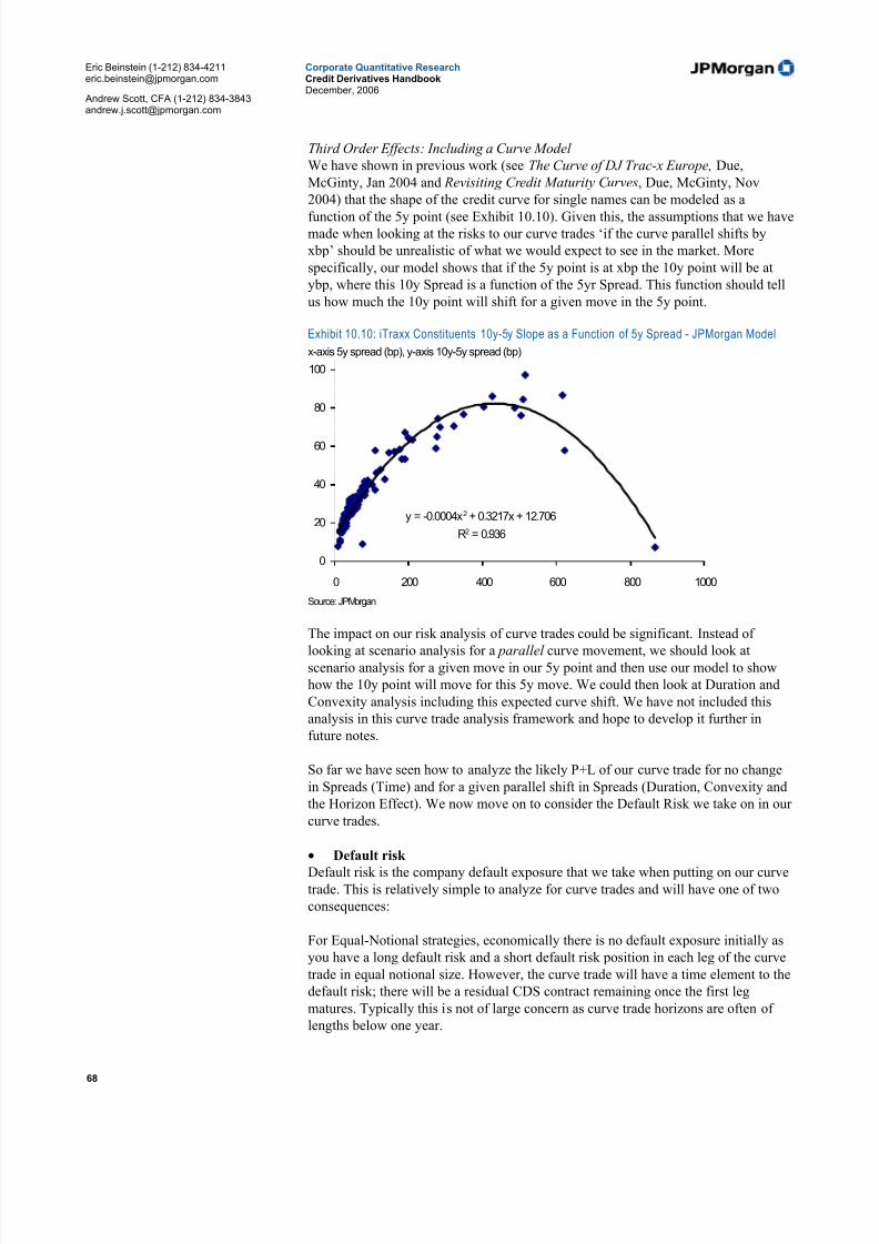
5/10/2018 JPM Credit Derivatives - slidepdf.com
http://slidepdf.com/reader/full/jpm-credit-derivatives-559e0102dc371 68/180
Eric Beinstein (1-212) [email protected]
Andrew Scott, CFA (1-212) [email protected]
Corporate Quantitative ResearchCredit Derivatives HandbookDecember, 2006
68
Third Order Effects: Including a Curve Model
We have shown in previous work (see The Curve of DJ Trac-x Europe, Due,
McGinty, Jan 2004 and Revisiting Credit Maturity Curves, Due, McGinty, Nov
2004) that the shape of the credit curve for single names can be modeled as a
function of the 5y point (see Exhibit 10.10). Given this, the assumptions that we havemade when looking at the risks to our curve trades ‘if the curve parallel shifts by
xbp’ should be unrealistic of what we would expect to see in the market. More
specifically, our model shows that if the 5y point is at xbp the 10y point will be at
ybp, where this 10y Spread is a function of the 5yr Spread. This function should tell
us how much the 10y point will shift for a given move in the 5y point.
Exhibit 10.10: iTraxx Constituents 10y-5y Slope as a Function of 5y Spread - JPMorgan Model
x-axis 5y spread (bp), y-axis 10y-5y spread (bp)
y = -0.0004x2 + 0.3217x + 12.706
R2 = 0.936
0
20
40
60
80
100
0 200 400 600 800 1000 Source: JPMorgan
The impact on our risk analysis of curve trades could be significant. Instead of
looking at scenario analysis for a parallel curve movement, we should look atscenario analysis for a given move in our 5y point and then use our model to show
how the 10y point will move for this 5y move. We could then look at Duration and
Convexity analysis including this expected curve shift. We have not included this
analysis in this curve trade analysis framework and hope to develop it further in
future notes.
So far we have seen how to analyze the likely P+L of our curve trade for no change
in Spreads (Time) and for a given parallel shift in Spreads (Duration, Convexity and
the Horizon Effect). We now move on to consider the Default Risk we take on in our
curve trades.
• Default risk
Default risk is the company default exposure that we take when putting on our curve
trade. This is relatively simple to analyze for curve trades and will have one of two
consequences:
For Equal-Notional strategies, economically there is no default exposure initially as
you have a long default risk and a short default risk position in each leg of the curve
trade in equal notional size. However, the curve trade will have a time element to the
default risk; there will be a residual CDS contract remaining once the first leg
matures. Typically this is not of large concern as curve trade horizons are often of
lengths below one year.

5/10/2018 JPM Credit Derivatives - slidepdf.com
http://slidepdf.com/reader/full/jpm-credit-derivatives-559e0102dc371 69/180
Eric Beinstein (1-212) [email protected]
Andrew Scott, CFA (1-212) [email protected]
Corporate Quantitative ResearchCredit Derivatives HandbookDecember, 2006
69
For strategies with differing notional weights in each leg (e.g. Duration-Weighted
trades) there will be default risk for the life of the curve trade which forms part of
the risks to the trade being profitable. Depending on their view on the underlying
credit, investors may not wish to put on a curve view if it results in a default
exposure they are uncomfortable with.
• Breakevens and curve steepening / flattening
The point of our framework for understanding the drivers of P+L in a curve trade is
to understand the likely profitability of curve trades given our view of future curve
moves. We therefore need to look at the breakeven curve movements that are needed
for our curve trade to be profitable.
In general, the Breakeven on a trade tells us what market move we need to ensure
that it makes zero profit. In that sense the Breakeven is the bottom line or our
minimum condition for putting on a trade. For example, if the 10y point is trading at
100bp and the 5y point is trading at 75bp, the ‘curve steepness’ (10y minus 5y
spread) is 25bp. An investor putting on a curve flattener trade, buying protection in
the 5y point and selling protection in the 10y point is working on the assumption that
the curve steepness will fall lower than 25bp. So, how much does the curve need to
flatten in order to breakeven on the trade over the trade horizon? If we calculate that
given all the other drivers of P+L in the trade, if the curve flattens 5bp the trade will
breakeven over three months, then 5bp is our bottom line flattening. An investor can
then assess whether this 5bp is really reasonable given their view of the company and
the market, or whether 5bp is too much of a move to expect and therefore the trade
will most likely lose money even if the curve does flatten a little.
We have two Breakevens we may want to look at for our trade:
Breakeven from Time
This is the breakeven curve change needed to ensure our curve trade MTM is zeroover the horizon given the Time (=Carry + Slide) P+L.
The Breakeven from Time is the curve change needed so that:
MTM Time, t to t+1 + MTM Curve, t to t+1 = 0 [4]
Or in long hand (for a curve flattener):
Carry t to t+1 + Slide t to t+1 + ∆S 5y.A5y,t+1.Ntnl 5y - ∆S 10y.A10y,t+1.Ntnl 10y = 0 [5]
Breakeven for a given spread change
The Breakeven for a given spread change gives the curve change needed to
breakeven from both the Time element and from the P+L effect of a given Spread
change.
Exhibit 10.11: Breakeven Curve Mov ements An alysis – Where Current 10y-5y Curve = 77.4bp, Slide Implied 10y-5y = 99.3bp
5y / 10y Curve Movement (in bp) Needed to Breakeven With a Duration-Weighted Flattener Over 3 Months
Chg in 5y 5Y (Slide Implied) 10Y Breakeven Breakeven Curve (10Y-5Y) Breakeven Curve Chg Breakeven Curve Chg(vs Slide Implied) bp bp bp bp (vs current curve) bp (vs Slide implied) bp-10 228 303 74.8 -2.7 -24.60 238 312 73.8 -3.6 -25.510 248 321 73.0 -4.5 -26.4
Source: JPMorgan
Bid-Offer Costs
In our analysis we simplify our Breakevens by ignoring bid-offer costs. In practice these tradingcosts also need to be consideredwhen accessing likely
profitability and Breakevens.
5/10/2018 JPM Credit Derivatives - slidepdf.com
http://slidepdf.com/reader/full/jpm-credit-derivatives-559e0102dc371 70/180
Eric Beinstein (1-212) [email protected]
Andrew Scott, CFA (1-212) [email protected]
Corporate Quantitative ResearchCredit Derivatives HandbookDecember, 2006
70
In our “Calculating Breakevens” discussion at the end of this section, we show that
we cannot find a single Breakeven number due to Convexity effects. Rather we
analyse Breakevens by setting the Spread at horizon of one leg of our trade and
calculating the curve move needed in the other leg to breakeven over the horizon.
Typically we set the shorter leg, for example we will set our 5y Spread and calculatehow the 10y point needs to move (and hence curve moves) to breakeven. This is
illustrated in Exhibit 10.11, for a 5y/10y trade where the 5y is currently at 200bp and
the Slide implied spread at horizon is 238bp. The grey row is our Breakeven from
Time, i.e. 5y is constant over the horizon and we therefore need 3.6bp of flattening of
our current curve to breakeven (column 5), which is really 25.5bp of flattening given
the implied curve due to Slide. The other rows are our Breakevens for a Given
Spread Change, for example if the 5y widens 10bp (to 248bp at horizon) then the 10y
needs to flatten 26.4pp for the trade to breakeven. This incorporates the Convexity
effects of a change in Spread.
“The Horizon Effect” discussion explains how we understand sensitivity analysis at
trade horizon where the Horizon Effect will mean we can have more or less market
exposure over the life of the trade – as we will see, this will help us understand our
Breakeven analysis at horizon.
Summary
In this section we have outlined our framework for properly analysing P+L in curve
trades looking at Time (Carry & Slide), Sensitivity Analysis (Duration, Convexity
and Horizon Effects), Default Risk and Breakevens. We now move on to common
curve trading strategies to see how we apply this in practice.
Curve trading strategies
Two-Legged Curve Trades
In the first part of this Section we outlined a framework for analyzing the drivers of
P+L in trades. We now turn to common curve trading strategies to understand whattypically are the largest factors that influence profitability in these trades. We
concentrate our analysis here on two-legged trades involving buying protection at
one point in the curve and selling protection at the second to express a view on the
way the shape of the curve will change. To express a view on the shape of the curve
with a two-legged trade, an investor can choose from: Equal-Notional Strategies
(Forwards), Duration-Weighted Strategies or Carry-Neutral Strategies.
1. Equal-Notional Strategies: Forwards
Equal-Notional curve trades involve buying and selling protection on equal notional
at two different maturities (i.e. points on the curve). For example, an investor can buy
protection on a notional of $10mm for 5 years and sell protection on a notional of
$10mm for 10 years (an equal-notional flattener). This trade is effectively Default Neutral for the life of the first (earlier maturity) leg of the trade – if a default happens
within the first 5 years, the investor will pay out on default for the 10y contract and
will receive back equal to this on the 5y contract.
We refer to a two-legged equal notional strategy as a Forward, as the position is
economically equivalent to having entered a forward-starting CDS contract (see
Trading Credit Curves I for a full explanation of this and the derivation of the
Forward equation). The 5y/5y Forward Spread (S5y/5y) is calculated as:
Curve Trade AnalysisFramework Summary:
1. Time: P+L from just time passing.
a) Carry b) Slide
2. Spread Changes: P+L if spreads change
a) Duration b) Convexityc) Horizon Effect
Default Risk
Breakevens
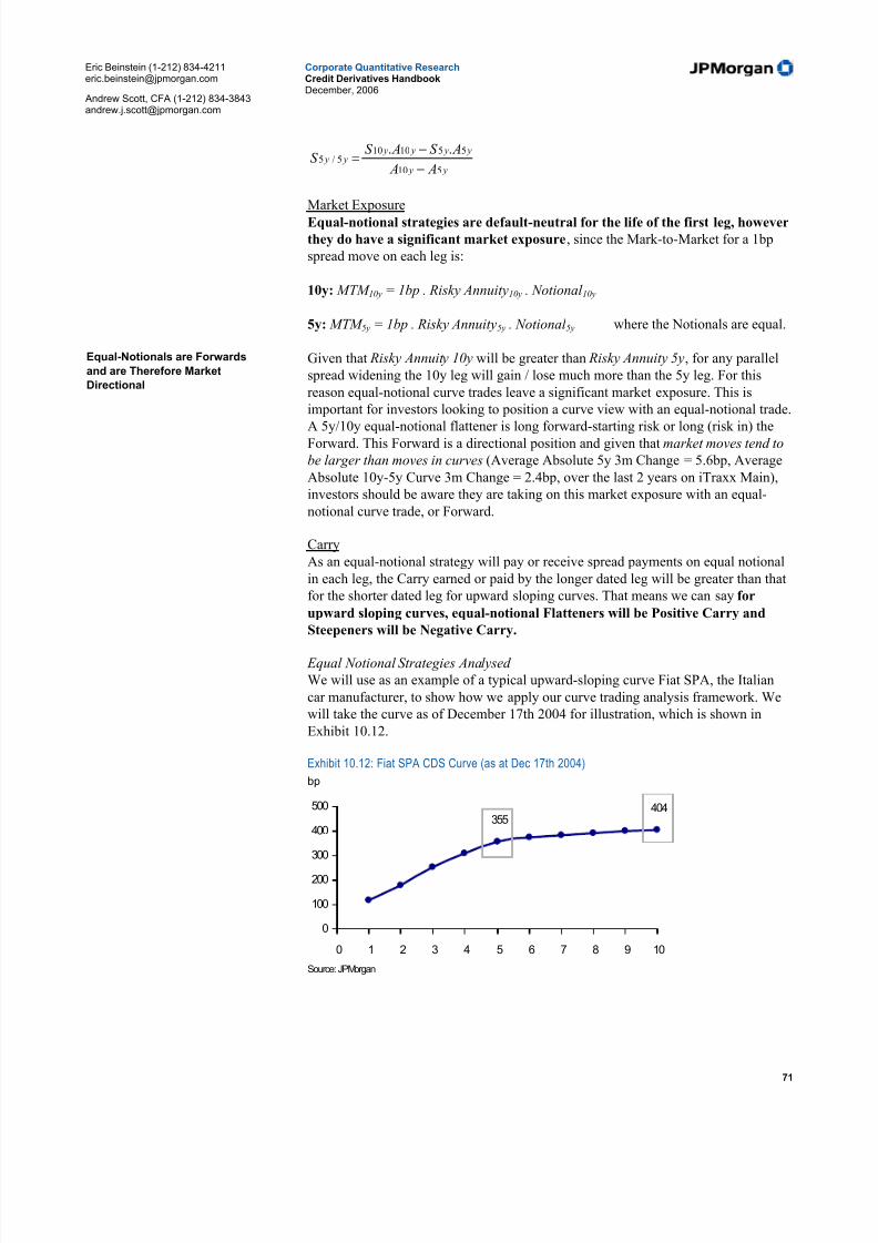
5/10/2018 JPM Credit Derivatives - slidepdf.com
http://slidepdf.com/reader/full/jpm-credit-derivatives-559e0102dc371 71/180
Eric Beinstein (1-212) [email protected]
Andrew Scott, CFA (1-212) [email protected]
Corporate Quantitative ResearchCredit Derivatives HandbookDecember, 2006
71
y y
y y y y y y
A A
AS AS S
510
5510105/5
..
−
−=
Market Exposure
Equal-notional strategies are default-neutral for the life of the first leg, however
they do have a significant market exposure, since the Mark-to-Market for a 1bp
spread move on each leg is:
10y: MTM 10y = 1bp . Risky Annuity10y . Notional 10y
5y: MTM 5y = 1bp . Risky Annuity5y . Notional 5y where the Notionals are equal.
Given that Risky Annuity 10y will be greater than Risky Annuity 5y, for any parallel
spread widening the 10y leg will gain / lose much more than the 5y leg. For this
reason equal-notional curve trades leave a significant market exposure. This is
important for investors looking to position a curve view with an equal-notional trade.
A 5y/10y equal-notional flattener is long forward-starting risk or long (risk in) theForward. This Forward is a directional position and given that market moves tend to
be larger than moves in curves (Average Absolute 5y 3m Change = 5.6bp, Average
Absolute 10y-5y Curve 3m Change = 2.4bp, over the last 2 years on iTraxx Main),
investors should be aware they are taking on this market exposure with an equal-
notional curve trade, or Forward.
Carry
As an equal-notional strategy will pay or receive spread payments on equal notional
in each leg, the Carry earned or paid by the longer dated leg will be greater than that
for the shorter dated leg for upward sloping curves. That means we can say for
upward sloping curves, equal-notional Flatteners will be Positive Carry and
Steepeners will be Negative Carry.
Equal Notional Strategies Analysed
We will use as an example of a typical upward-sloping curve Fiat SPA, the Italian
car manufacturer, to show how we apply our curve trading analysis framework. We
will take the curve as of December 17th 2004 for illustration, which is shown in
Exhibit 10.12.
Exhibit 10.12: Fiat SPA CDS Curve (as at Dec 17th 2004)
bp
404355
0
100
200
300
400
500
0 1 2 3 4 5 6 7 8 9 10 Source: JPMorgan
Equal-Notionals are Forwards
and are Therefore Market
Directional
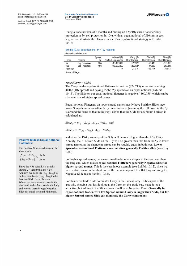
5/10/2018 JPM Credit Derivatives - slidepdf.com
http://slidepdf.com/reader/full/jpm-credit-derivatives-559e0102dc371 72/180
Eric Beinstein (1-212) [email protected]
Andrew Scott, CFA (1-212) [email protected]
Corporate Quantitative ResearchCredit Derivatives HandbookDecember, 2006
72
Using a trade horizon of 6 months and putting on a 5y/10y curve flattener (buy
protection in 5y, sell protection in 10y), with an equal notional of $10mm in each
leg, we can illustrate the characteristics of an equal-notional strategy in Exhibit
10.13:
Exhibit 10.13: Equal Notional 5y / 10y Flattener
6 month trade horizon
Spread Notion al ($) Carry ($) Slide ($) Time ($Tenor Position bp (Default Exposure) Over Horizon Over Horizon Over Horizon
5Y Buy Protection 355 -10,000,000 -177,972 -75,419 -253,39010Y Sell Protection 404 +10,000,000 202,687 14,660 217,347Flatten er 0 24,715 -60,759 -36,043
Source: JPMorgan
Time (Carry + Slide)
The Carry on the equal-notional flattener is positive ($24,715) as we are receiving
404bp (10y spread) and paying 355bp (5y spread) on an equal notional (Exhibit
10.13). The Slide on our equal-notional flattener is negative (-$60,759) which can be
characteristic of higher spread names.
Equal-notional Flatteners on lower spread names mostly have Positive Slide since
lower Spread curves are often fairly linear in shape (meaning the roll down in the 5y
is around the same as that in the 10y). Given that the Slide for a 6 month horizon is
calculated as:
Slide5y = (S 5y – S 4.5y ) . A4.5y . Ntnl 5y and
Slide10y = (S 10y – S 9.5y ) . A9.5y . Ntnl 10y
and since the Risky Annuity of the 9.5y will be much higher than the 4.5y RiskyAnnuity, the P+L from Slide on the 10y will be greater than that from the 5y in lower
spread names, as the change in spread can be roughly equal in both legs. Lower
Spread equal-notional Flatteners are therefore generally Positive Slide (see Grey
Box.)
For higher spread names, the curve can often be much steeper in the short end than
the long end, which makes equal-notional Flatteners generally Negative Slide for
higher spread names. This is the case in our example (see Exhibit 10.12), since we
have a steep curve in the short end of the curve compared to a flat long end we get a
Negative Slide (as in Exhibit 10.13).
For this curve trade Slide dominates Carry in the Time (Carry + Slide) part of the
analysis, showing that just looking at the Carry on this trade may make it look attractive, but adding in the Slide shows it will have Negative Time. Generally for
equal-notional trades, with low Spread names Carry is larger than Slide, but for
higher Spread names Slide can dominate the Carry component.
Positive Slide in Equal NotionalFlatteners:
The positive Slide condition can beshown to be:
y
y
y y
y y
A
A
S S
S S
5.9
5.4
5.45
5.910
)(
)(>
−
−
Since the 9.5y Annuity is usuallyaround 2 × larger that the 4.5yAnnuity, we need the (S5y - S4.5y) to
be less than twice (S10y - S9.5y) to bePositive Slide for a Flattener.Where we have a steep curve in the
short-end and a flat curve in the longend we can therefore get NegativeSlide for equal-notional Flatteners.

5/10/2018 JPM Credit Derivatives - slidepdf.com
http://slidepdf.com/reader/full/jpm-credit-derivatives-559e0102dc371 73/180
Eric Beinstein (1-212) [email protected]
Andrew Scott, CFA (1-212) [email protected]
Corporate Quantitative ResearchCredit Derivatives HandbookDecember, 2006
73
Sensitivity to Spread Changes (Duration & Convexity)
Having understood the Time component if nothing else changes, we now need to
understand how our trade will perform should spreads change – we first look at the
sensitivity to immediate or instantaneous changes in spreads.
Exhibit 10.14: Sensitiv ity to Instant aneous Spread Changes
-40bp Spread Chg -20bp Spread Chg 0bp Spread Chg 20bp Spread Chg 40bp Spread Chg
1) MTM 5Y (Buy) -172,604 -85,614 0 84,262 167,1922) MTM 10Y (Sell) 271,344 133,728 0 -129,958 -256,2603) Curve Trade 98,740 48,113 0 -45,696 -89,0684) Spread Chg × Current Annuity 5Y -169,869 -84,934 0 84,934 169,8695) Spread Chg × Current Annuity 10Y 263,646 131,823 0 -131,823 -263,6466) Curve Trade 93,778 46,889 0 -46,889 -93,7787) Convexity Effect (Row 3 – Row 6) 4,962 1,224 0 1,193 4,709
Source: JPMorgan
Exhibit 10.14 shows the MTM of our trade to parallel spread changes. We first look
at the actual MTM of the trade in rows 1-3, where we can see that this trade has a
large directionality to it. Exhibit 10.15 shows this graphically and we have a negative
MTM for spread widening and positive MTM for spread tightening. Given the5y/10y equal-notional Flattener is long Forward-starting risk, we should imagine a
market-directionality to this position. Investors looking to position for curve
moves using an equal-notional strategy, should be aware they are taking this
market risk position by trading the Forward.
Rows 4-7 of Exhibit 10.14 show the Convexity effect in the trade, which is much
smaller compared to the first order effect of spreads moving. In order to illustrate
Convexity, we keep the Risky Annuities constant and look at the predicted MTM
from the spread change and compare that to the actual MTM to get the MTM gain /
loss from changes in Risky Annuity, i.e. the Convexity. This trade has Positive
Convexity as it has a relative MTM gain for spreads tightening or widening due to
changes in the Risky Annuities (Durations). Equal-Notional Flatteners have
Positive Convexity and Steepeners have Negative Convexity.
Exhibit 10.15: Sensitivi ty to Instant aneous Spread Changes
x-axis: bp spread changes, y-axis: MTM ($)
-100,000
-50,000
0
50,000
100,000
150,000
-40 -20 0 20 40
Source: JPMorgan
Sensitivity Analysis at Horizon
We can also analyse our trade’s sensitivity to spread changes at horizon. This is a
more complex analysis as the Horizon Effect on the trade affects our market
exposure over the life of the trade, discussed later. Exhibit 10.16 shows us the
sensitivity of the position to a 20bp move in spreads wider or tighter at horizon
(Carry not included). The large Negative Slide (-$60,759) means that we have a
negative MTM for a spread widening and 20bp tightening at horizon, although we
have a positive MTM if spreads tighten 40bp at horizon (row 3). If we look at the
MTM net of Slide (row 4) we can see the market position that we have in the curve
trade. In order to look at just the market position we gain over time, we finally look

5/10/2018 JPM Credit Derivatives - slidepdf.com
http://slidepdf.com/reader/full/jpm-credit-derivatives-559e0102dc371 74/180
Eric Beinstein (1-212) [email protected]
Andrew Scott, CFA (1-212) [email protected]
Corporate Quantitative ResearchCredit Derivatives HandbookDecember, 2006
74
at the MTM effect less the Instantaneous MTM, in order to get just our Horizon
Effect.
Exhibit 10.16: Sensitivity Analysis AT HORIZON for Equal Notio nal Flattener (Carry Not Included)
-40bp Spread Chg -20bp Spread Chg 0bp Spread Chg 20bp Spread Chg 40bp Spread Chg1) MTM 5Y (Buy) -233,428 -153,783 -75,419 2,103 78,3772) MTM 10Y (Sell) 275,938 143,497 14,660 -110,704 -232,6723) Curve Trade MTM at Horizon 42,509 -10,286 -60,759 -108,601 -154,2954) Curve Trade MTM at Horizon minus Slide 103,268 50,473 0 -47,842 -93,5365) Instantaneous MTM 98,740 48,113 0 -45,696 -89,0686) Horizon Effect (Row 4 - Row 5) 4,528 2,360 0 -2,146 -4,468
Source: JPMorgan
In this case, we have a larger risk position due to the Horizon Effect and so lose more
for spread widening and gain for spread tightening at horizon (as shown in the last
row of Exhibit 10.16).
Equal Notional 5y/10y Flatteners generally have increasing risk over the life of the
trade due to the Horizon Effect and Steepeners have decreasing risk due to the
Horizon Effect. Default Risk
This trade has equal notional exposure in each leg so is effectively Default-Neutral
over the trade horizon.
Breakeven Analysis
Putting all this analysis together, the bottom line is whether our curve will flatten
enough to at least breakeven. Exhibit 10.17 shows this Breakeven analysis. Given we
have a flattener on, if the spread curve is constant (i.e. the 5y leg rolls down the
current spread curve to its Slide-implied level) we need the 10y point to move to
397bp, as in Row 3. This looks like a steepening of 11.7bp vs the current 10y-5y
Spread, but is really a 5.4bp curve flattening versus the Slide-implied curve steepness
(as shown in the final column). The shaded row shows this Breakeven for Time. This
intuitively makes sense as we need some curve flattening to counterbalance thenegative Time (Slide –Carry). If Spreads do widen in the 5y point by 20bp then we
need curves to flatten 13.4bp to breakeven on the trade over the 6 month horizon as
we have greater negative MTM for spread widening due to the Horizon Effect
making the trade longer risk. Therefore, we need a larger flattening to breakeven.
The key decision in putting on this trade is therefore whether we can expect -5.4bp if
spreads are unchanged or if we think spreads are widening 20bp do we think curves
will flatten 13.4bp.
Exhibit 10.17: Breakevens for Equal-Notion al Flattener
Current 10y-5y curve = 49bp, Slide Implied 10y-5y curve = 66bp.
Chg in 5y 5Y (Slide Implied) 10Y Breakeven Breakeven Curve (10Y-5Y) Breakeven Curve Chg Breakeven Curve Chg(vs Slide Implied) bp bp bp bp (vs current curve) bp (vs Slide implied) bp
-40 296 373 77.2 27.9 10.7
-20 316 385 69.1 19.8 2.60 336 397 61.0 11.7 -5.4
20 356 409 53.0 3.7 -13.440 376 421 45.1 -4.2 -21.3
Source: JPMorgan

5/10/2018 JPM Credit Derivatives - slidepdf.com
http://slidepdf.com/reader/full/jpm-credit-derivatives-559e0102dc371 75/180
Eric Beinstein (1-212) [email protected]
Andrew Scott, CFA (1-212) [email protected]
Corporate Quantitative ResearchCredit Derivatives HandbookDecember, 2006
75
Trade Performance Analysis
We can finally look at the likely trade performance for different spread levels in our
5y and 10y legs over the horizon in Exhibit 10.18.
Exhibit 10.18: Trade Performance An alysisVertical spreads are centered around Slide Implied 5y Spreads (bp) at horizon, Horizontal are centered
around 10y Spreads at horizon (bp). Data is trade MTM ($) incl. Carry at horizon
Current 10y at Horizon**362 382 402 422 442
296 70,765 -60,563 -190,330 -318,544 -445,212316 147,036 16,917 -111,651 -238,676 -364,166
Current 5y at Horizon* 336 221,867 92,929 -36,043 -160,337 -284,679356 295,295 167,511 41,254 -83,484 -206,707376 367,359 240,703 115,560 -8,074 -130,208
Source: JPMorgan. * Slide Implied spread of current 5y at Horizon, ** Slide Implied spread of current 10y at Horizon.
We can see that this trade performs well for curve flattening (10y spread decreases or
5y spread increases) and due to the Negative Time, if spreads are unchanged it loses
money over the horizon. This is what we would expect from a flattener trade – it profits as the curve flattens and will lose money increasingly as the curve steepens.
Importantly we now have a way to accurately assess this P+L and so can take a view
on whether we think the curve will flatten enough to make the trade profitable.
Summary of Equal Notional Characteristics
The P+L and Sensitivity characteristics for equal-notional curve trades (for 5y/10y trades on typical upward sloping curves)
are summarised in Exhibit 10.19 and Exhibit 10.20.
Exhibit 10.19: P+L Characteristi cs for Equal Notional Curv e Trades
Carry Slide Dominant Time Effect (Carry or Slide) 1bp Instantaneous Widening DefaultFlattener Positive Low Spread = Positive Low Spread = Carry MTM Loss Neutral
High Spread = Negative High Spread = Slide
Steepener Negative Low Spread = Negative Low Spread = Carry MTM Gain NeutralHigh Spread = Positive High Spread = Slide
Source: JPMorgan
Exhibit 10.20: Sensiti vity Summ ary for Equal Notional Curve Trades
1bp Instantaneous Widening Convexity from Spread Chg Horizon Impact for 5y/10y Trade
Flattener MTM Loss Positive Longer risk over horizonSteepener MTM Gain Negative Shorter risk over horizon
Source: JPMorgan

5/10/2018 JPM Credit Derivatives - slidepdf.com
http://slidepdf.com/reader/full/jpm-credit-derivatives-559e0102dc371 76/180
Eric Beinstein (1-212) [email protected]
Andrew Scott, CFA (1-212) [email protected]
Corporate Quantitative ResearchCredit Derivatives HandbookDecember, 2006
76
2. Duration-weighted strategies
We have seen that a major feature of equal-notional trades is the large MTM effect
from parallel curve moves which may not be particularly desirable for an investor
who is just trying to express a view on the relative movement of points in the curve.In order to immunize curve trades for parallel curve moves we can look to weight the
two legs of the trade so that for a 1bp parallel move in spreads, the Mark-to-Market
on each leg is equal – we call this Duration-Weighting the trade. We can do this by
fixing the Notional of one leg of the trade, for example set the 10y Notional to
$10mm, and can then solve to find the Notional of the 5y leg so that the trade is
MTM neutral for a 1bp move in Spreads.
For a curve trade at Par, the Mark-to-Market of each leg for a 1bp shift in Spreads isgiven by16:
MTM 10y = 1bp.Duration10y.Ntnl 10y, and equivalent for the 5y
The Duration-Weighted trade adjusts the Notionals so that:
MTM 10y = MTM 5y for a 1bp parallel move in spreads,
i.e. 1bp . Duration10y . Ntnl 10y = 1bp . Duration5y . Ntnl 5y
y y
y y Ntnl
Duration
Duration Ntnl 10
5
105 .=
Default Exposure
As we have adjusted the 5y notional exposure to be larger than the 10y, we now have
default exposure over the life of the trade as a default in the first 5 years will mean
paying out or receiving (1-Recovery) on a larger notional.
Duration-weighted strategies analysed
We continue with our Fiat SPA example to see how we should analyse our Duration-
Weighted trade whose structure is shown in Exhibit 10.21.
Time (Carry & Slide)
Looking first at our Carry in Exhibit 10.21, we can see that we have Negative Carry
(-$73,535) over the trade horizon. Duration-weighted flatteners are typically
Negative Carry unless for very steep curves (see the Grey Box for an explanation
of this).
Exhibit 10.21: Duration-Weighted 5y / 10y Flattener
6 month trade horizon
Tenor Positi on Spread Notion al ($) Carry ($) Slide ($) Time ($bp (Default Exposure) Over Horizon Over Horizon Over Horizon
5Y Buy Protection 355 -15,520,593 -276,223 -117,054 -393,2710Y Sell Protection 404 +10,000,000 202,687 14,660 217,34Flatten er -5,520,593 -73,535 -102,394 -175,930
Source: JPMorgan
16See Trading Credit Curves I for a discussion of Risky Duration and Risky Annuity. For a
curve trade at Par and for a 1bp change in spreads only the MTM can be expressed using theRisky Duration, for other moves we need to use the Risky Annuity.

5/10/2018 JPM Credit Derivatives - slidepdf.com
http://slidepdf.com/reader/full/jpm-credit-derivatives-559e0102dc371 77/180
Eric Beinstein (1-212) [email protected]
Andrew Scott, CFA (1-212) [email protected]
Corporate Quantitative ResearchCredit Derivatives HandbookDecember, 2006
77
Positive Carry Duration-Weighted Flatteners
To Duration-Weight a trade we set: y y
y y Ntnl
Duration
Duration Ntnl 10
5
105 .=
Given that the Carry in each leg is given by (e.g. for the 5y): Carry5y = S 5y . Ntnl 5y . Horizon
We can see that: Horizon Ntnl Duration
DurationS Carry y
y
y y y ... 10
5
1055 =
For a Duration-Weighted Flattener to be Positive Carry, we need: y
y y y
Duration
DurationS S
5
10510 .>
which is generally not the case unless curves are very steep.
We also have significant Negative Slide over the horizon as the 5y part of the curve
is much steeper than the 10y part and therefore there is larger Negative Slide here, as
Exhibit 10.12 shows.
Generally for Duration-Weighted Flatteners Slide is Negative and for
Steepeners Slide is Positive. This is because the Risky Annuity × Notional is
approximately equal in both legs (the Duration-Weighting condition), so the MTM
due to Slide is largely about whether the spread change is greater in the shorter leg or
the longer leg. As most curves are steeper in the short end, this means the short end
has a greater MTM from Slide, hence flatteners have negative Slide and steepeners
have positive Slide.
For Duration-Weighted trades Slide dominates Carry in the Time consideration
meaning Carry alone is not sufficient to assess likely profitability of a trade in an
unchanged spread environment. The Duration-Weighted 'holy grail' of the Positive
Carry Flattener will most likely be P+L negative if curves remain unchanged asSlide will be negative and will dominate the Carry effect.
Sensitivity to Spread Changes (Duration & Convexity)
In terms of parallel curve movements (Duration effect) we have structured the trade
so that it should be MTM neutral for a 1bp parallel change in spreads of the curve.
However, there is also a Convexity impact from Spread widening to understand.
Exhibit 10.22 shows this Convexity impact for larger spread changes on our
Duration-Weighted Flattener. We can see that for large spread widening or tightening
the position has a positive MTM. We call this Positive Convexity and Duration-
Weighted Flatteners usually have Positive Convexity and Steepeners haveNegative Convexity (see the first section of this note, The Drivers of P+L in Curve
Trades, for an explanation of this)

5/10/2018 JPM Credit Derivatives - slidepdf.com
http://slidepdf.com/reader/full/jpm-credit-derivatives-559e0102dc371 78/180
Eric Beinstein (1-212) [email protected]
Andrew Scott, CFA (1-212) [email protected]
Corporate Quantitative ResearchCredit Derivatives HandbookDecember, 2006
78
Exhibit 10.22: Convexity for Duration-Weighted Flattener
x-axis: parallel chg (bp), y-axis: P+L at horizon from curve position
0
1,000
2,000
3,000
4,000
-40 -20 0 20 40
Source: JPMorgan
Exhibit 10.23 shows this analysis in more detail, where Row 3 has the actual MTM
from (instantaneous) spread moves and Row 6 shows the expected MTM from spread
moves using the current Risky Annuities – given we are Duration-Weighted this is
zero. The Convexity effect (Row 7) is then just the actual MTM minus the expected
MTM using the current Risky Annuities.
Exhibit 10.23: Sensitivity Analysis for Spread Changes
-40bp Spread Chg -20bp Spread Chg 0bp Spread Chg 20bp Spread Chg 40bp Spread Chg
1) MTM 5Y (Buy) -267,892 -132,879 0 130,779 259,4922) MTM 10Y (Sell) 271,344 133,728 0 -129,958 -256,2603) Curve Trade 3,452 849 0 821 3,2324) Spread Chg × Current Annuity 5Y -263,646 -131,823 0 131,823 263,6465) Spread Chg × Current Annuity 10Y 263,646 131,823 0 -131,823 -263,6466) Curve Trade 0 0 0 0 07) Convexity Effect (Row 3 – Row 6) 3,452 849 0 821 3,232
Source: JPMorgan
Sensitivity Analysis at Horizon
Having seen our sensitivity to instantaneous spread changes, we can now look at our
sensitivities to spread changes at the horizon of the trade. Exhibit 10.24 shows the
MTM (without Carry) from the trade in both a Parallel Widening and Tightening at
horizon. The trade has negative MTM in both, which is mostly due to the large
negative Slide that we saw in this trade. However, the sensitivity to spread widening
and tightening at the trade horizon also contains a Horizon Effect. As we discuss in
“The Horizon Effect”, our Duration-Weighted trade will become market directional
over its life due to this Effect. We can see this in Exhibit 10.24 as we get a market
directional position where we have relative positive MTM for spreads tightening and
negative for spreads widening (row 7 of Exhibit 10.24).
Exhibit 10.24: P+L Sensitivity A nalysis f or Duration-Weighted Flattener
-40bp Spread Chg -20bp Spread Chg 0bp Spread Chg 20bp Spread Chg 40bp Spread Chg1) MTM 5Y (Buy) -362,295 -238,680 -117,054 3,264 121,6452) MTM 10Y (Sell) 275,938 143,497 14,660 -110,704 -232,6723) Curve Trade MTM at Horizon -86,357 -95,183 -102,394 -107,440 -111,0264) Curve Trade MTM at Horizon minus Slide 16,037 7,211 0 -5,045 -8,6325) Instantaneous MTM 3,452 849 0 821 3,2326) Horizon Effect (Row 4 – Row 5) 12,585 6,363 0 -5,867 -11,864
Source: JPMorgan
Exhibit 10.25 illustrates the Horizon Effect graphically – the full workthrough of this
is detailed later in our discussion.

5/10/2018 JPM Credit Derivatives - slidepdf.com
http://slidepdf.com/reader/full/jpm-credit-derivatives-559e0102dc371 79/180
Eric Beinstein (1-212) [email protected]
Andrew Scott, CFA (1-212) [email protected]
Corporate Quantitative ResearchCredit Derivatives HandbookDecember, 2006
79
Exhibit 10.25: Sensitivity Analysis at Horizon (less Slide)
x-axis: parallel chg (bp), y-axis: P+L at horizon from curve position at horizon less Slide
-10,000
-5,000
0
5,000
10,000
15,000
20,000
-40 -20 0 20 40
Source: JPMorgan
5y/10y Duration-Weighted Flatteners generally get longer risk over the horizon of the trade and steepeners get shorter risk over the horizon.
Default Risk
We can see from Exhibit 10.21 that we are short default risk for the trade horizon, as
we have bought protection on a larger notional than we sold protection on, meaning
we benefit if there is a default in the first 5 years. Duration-Weighted Flatteners
will always be short default risk as they will always have a larger notional in the
shorter leg in order to balance the Duration effects; Steepeners will be long
default risk.
Breakevens
Once we have done all of our analysis, we can finally look at the Breakevens for our
Duration-Weighted Flattener in Exhibit 10.26. The shaded row shows the Breakevencurve move needed to compensate for the unchanged spread scenario, i.e. to
compensate for the Time effect. Due to the large Slide effect in Time, we need
27.2bp of curve flattening to Breakeven from Time in this trade (shaded row, column
6). We can also see the Breakeven curve moves needed for spread widening or
tightening at the 5y point (more on how we analyse Breakevens at the end of the
Section). As our Horizon Effect makes us longer risk over the life of the trade, we
need increasing flattening if spreads widen at horizon, as Exhibit 10.26 shows.
Exhibit 10.26: Breakeven for Duration-Weighted Flattener
Current 10y-5y curve = 49bp, Slide Implied 10y-5y curve = 66bp.
Chg in 5y 5Y (Slide Implied) 10Y Breakeven Breakeven Curve (10Y-5Y) Breakeven Curve Chg Breakeven Curve Chg(vs Slide Implied) bp bp bp bp (vs current curve) bp (vs Slide implied) bp
-40 296 339 43.4 -5.9 -23.1-20 316 357 41.2 -8.1 -25.2
0 336 375 39.3 -10.0 -27.220 356 393 37.6 -11.7 -28.940 376 412 36.0 -13.3 -30.4
Source: JPMorgan
Exhibit 10.27 analyses the trade performance at horizon, where we can see that our
Duration-Weighted flattener will only perform if we have larger curve flattening due
to the large negative Time for this trade. For example, if the 5y point is unchanged
(and we therefore move to the Slide Implied 5y of 336bp over the horizon, shaded
row), the 10y point needs to flatten 40bp for the trade to breakeven. A trader or
investor looking to put on this flattener would need to decide whether they think that
this magnitude of flattening is likely in order to want to put on this trade.

5/10/2018 JPM Credit Derivatives - slidepdf.com
http://slidepdf.com/reader/full/jpm-credit-derivatives-559e0102dc371 80/180
Eric Beinstein (1-212) [email protected]
Andrew Scott, CFA (1-212) [email protected]
Corporate Quantitative ResearchCredit Derivatives HandbookDecember, 2006
80
Exhibit 10.27: Trade Performance An alysis
Vertical spreads are centered around Slide Implied 5y Spreads (bp)at horizon, Horizontal are centered
around 10y Spreads at horizon (bp). Data is trade MTM ($) incl. Carry at horizon
Current 10y at Horizon**362 382 402** 422 442
296 -153,750 -285,390 -415,478 -544,025 -671,040316 -34,210 -164,528 -293,301 -420,538 -546,249
Current 5y at Horizon* 336* 83,078 -45,954 -175,930 -299,418 -423,864356 198,174 70,393 -55,862 -180,596 -303,817376 311,138 184,574 59,526 -64,010 -186,042
Source: JPMorgan. * Slide Implied spread of current 5y at Horizon, ** Slide Implied spread of current 10y at Horizon.
Summary of Duration-Weighted Characteristics
The P+L and Sensitivity characteristics for Duration-Weighted curve trades (for 5y/10y trades on typical upward sloping
curves) are summarised in Exhibit 10.28 and Exhibit 10.29.
Exhibit 10.28: P+L Characteristic s for Durati on-Weighted Trades
Carry Slide Dominant Time Effect (Carry or Slide) 1bp Instantaneous Widening DefaultFlattener Generally Negative Generally Negative Generally Slide MTM Neutral Short RiskSteepener Generally Positive Generally Positive Generally Slide MTM Neutral Long Risk
Source: JPMorgan
Exhibit 10.29: Sensitiv ity Summary fo r Duration-Weighted Curve Trades
1bp Instantaneous Widening Convexity from Spread Chg Horizon Impact for 5y/10y Trade
Flattener MTM Neutral Positive Longer risk over horizonSteepener MTM Neutral Negative Shorter risk over horizon
Source: JPMorgan
3. Carry-neutral strategiesA third way of looking to structure two-legged curve trades in credit is to look at
putting on these trades Carry Neutral. By 'Carry Neutral' we mean that the income
earned on both legs is the same over the trade horizon.
We define the Carry on a 5y CDS contract as: Carry5y = S 5y . Horizon . Ntnl 5y
Where,S 5y = Par Spread on 5y maturity CDS contract
Horizon = Year fraction of trade horizon
Ntnl 5y = Notional of 5y CDS contract
The Carry-Neutral condition is that: Carry Legx = Carry Legy
For a 5y / 10y flattener (buy protection 5y, sell protection 10y):
S 5y.Horizon.Ntnl 5y = S 10y.Horizon.Ntnl 10y
Therefore, to be Carry-Neutral where we want to buy $10m of notional protection in
the 10y, we need to sell protection on the following notional in the 5y leg:
y y
y y Ntnl
S
S Ntnl 10
5
105 .=

5/10/2018 JPM Credit Derivatives - slidepdf.com
http://slidepdf.com/reader/full/jpm-credit-derivatives-559e0102dc371 81/180
Eric Beinstein (1-212) [email protected]
Andrew Scott, CFA (1-212) [email protected]
Corporate Quantitative ResearchCredit Derivatives HandbookDecember, 2006
81
Carry-Neutral strategies can be useful for investors who want to avoid P+L from
interim cashflows and would like pure P+L from curve movements.
Carry-neutral strategies with our analysis framework
Without going through all of the features of Carry-Neutral strategies, we can see thatthe Carry-Neutral trade can have some of the characteristics to Duration-Weighted
strategies. We use our Fiat SPA trade as before to briefly show the characteristics of
Carry-Neutral Flattener trades.
Time (Carry & Slide)
Looking at Exhibit 10.30, we can see that we have zero Carry over the horizon (by
definition) and negative Slide of -$71,232, which will be the Time (as Carry is zero).
Exhibit 10.30: Time Analysis fo r Carry-Neutral Trade
Spread Notion al ($) Carry ($) Slide ($) Time ($Tenor Position bp (Default Exposure) Over Horizon Over Horizon Over Horizon
5Y Buy Protection 355 -11,388,732 -202,687 -85,892 -288,58
10Y Sell Protection 404 +10,000,000 202,687 14,660 217,34Flattener -1,388,732 0 -71,232 -71,232
Source: JPMorgan
Sensitivity to spread changes (Duration & Convexity)
We can see that our Carry-Neutral strategy is long risk for spread moves (see Row 3
of Exhibit 10.31) and has negative MTM for spread widening and positive MTM for
spread tightening. If S10y/S5y is less than Duration10y / Duration5y then a Carry-Neutral
flattener will be long spread risk as it will have bought less notional protection in the
5y leg than it needs to be Duration-Weighted so it will have negative MTM for
spread widening. Carry-Neutral trades on low spread names tend to be mixed in
terms of being long or short spread risk; higher spread names tend to be long
risk. Additionally, this has Positive Convexity and therefore loses relatively less for spread widening and makes relatively more for spread tightening (Row 7).
The Horizon Effect for Carry-Neutral flatteners also makes the position longer risk,
meaning at horizon we have a negative MTM for spreads widening (relative to the
start) and positive MTM for spreads tightening (relative to the start).
Exhibit 10.31: P+L Analysis fo r Carry-Neutral Flattener
-40bp Spread Chg -20bp Spread Chg 0bp Spread Chg 20bp Spread Chg 40bp Spread Chg
1) MTM 5Y (Buy) -196,574 -97,504 0 95,963 190,4112) MTM 10Y (Sell) 271,344 133,728 0 -129,958 -256,2603) Curve Trade 74,770 36,224 0 -33,994 -65,8504) Spread Chg × Current Annuity 5Y -193,459 -96,729 0 96,729 193,4595) Spread Chg × Current Annuity 10Y 263,646 131,823 0 -131,823 -263,646
6) Curve Trade 70,187 35,094 0 -35,094 -70,1877) Convexity Effect (Row 3 – Row 6) 4,582 1,130 0 1,099 4,338
Source: JPMorgan
Default risk
For upward sloping curves, Carry-Neutral Flatteners will be short default risk
and Steepeners will be long default risk. We tend to see lower Spread names
having a larger short default risk position than higher Spread names, as the ratio of
spreads between 10y and 5y is generally higher for lower Spread names as curves are
more linear.

5/10/2018 JPM Credit Derivatives - slidepdf.com
http://slidepdf.com/reader/full/jpm-credit-derivatives-559e0102dc371 82/180
Eric Beinstein (1-212) [email protected]
Andrew Scott, CFA (1-212) [email protected]
Corporate Quantitative ResearchCredit Derivatives HandbookDecember, 2006
82
Summary of Carry-Neutral Characteristics
The P+L and Sensitivity characteristics for Carry-Neutral curve trades (for 5y/10y trades on typical upward sloping curves)
are summarised in Exhibit 10.32 and Exhibit 10.33.
Exhibit 10.32: P+L Characteristics for Carry-Neutral Trades
Carry Slide Dominant Time Effect (Carry or Slide) 1bp Instantaneous Widening DefaultFlattener Zero (by definition) Negative Slide (by definition) Lower Spread: Mixed Short Risk
Higher Spread: Generally NegativeSteepener Zero (by definition) Positive Slide (by definition) Lower Spread: Mixed Long Risk
Higher Spread: Generally Positive
Source: JPMorgan
Exhibit 10.33 : Sensitivity Summary fo r Carry-Neutral Curve Trades
1bp Instantaneous Widening Convexity from Spread Chg Horizon Impact for 5y/10y TradeFlattener Lower Spread: Mixed Positive Longer risk over horizon
Higher Spread: Generally NegativeSteepener Lower Spread: Mixed Negative Shorter risk over horizon
Higher Spread: Generally PositiveSource: JPMorgan
Different ways of calculating slide
We talk of Slide as the effect from moving down the credit curve over time assuming
that the credit curve is unchanged . However, there are two ways that we could
understand that the credit curve is unchanged which would give rise to two ways of
calculating Slide:
i) Hazard Rates / Spreads for a given tenor are kept constant17
ii) Hazard Rates for a given calendar point are kept constant
i) Hazard rates / spreads for a given tenor constant
Keeping spreads constant for each tenor means that if the 5y point is currently at
100bp (for maturity in March 2011), the 5y point will still be at 100bp at horizon. If
our trade horizon is 1 year and we have a 5y contract, our March 2011 maturity will
become a 4y over the horizon and therefore rolls down the spread curve to be at 90bp
(e.g.). This will mean that the survival probability is higher for this shorter maturity
and a long risk CDS position will have a positive MTM equal to: - (Spread 5y –
Spread 4y) × Risky Annuity 4y × Notional.
We can illustrate what this Slide means in terms of default probabilities and hazard
rates in Exhibit 10.34 and Exhibit 10.35.
17See Trading Credit Curves I for a full discussion of the role of hazard rates in CDS pricing.

5/10/2018 JPM Credit Derivatives - slidepdf.com
http://slidepdf.com/reader/full/jpm-credit-derivatives-559e0102dc371 83/180
Eric Beinstein (1-212) [email protected]
Andrew Scott, CFA (1-212) [email protected]
Corporate Quantitative ResearchCredit Derivatives HandbookDecember, 2006
83
Exhibit 10.34: Initial Hazard Rates at Inception of CDS Contract
Hazard Rates, %
Mar-06 Mar-07 Mar-08 Mar-09 Mar-10
1.00%
2.00%
3.00%
4.00%
1Y 2Y 3Y 4Y 5Y
Calendar Dates:
Tenors:
Maturity
Source: JPMorgan
Exhibit 10.35: 1 Year Slide - Hazard Rates Constant at Tenors
Hazard Rates, %
Mar-07 Mar-08 Mar-09 Mar-10
1.00%
2.00%
3.00%
4.00%
1Y 2Y 3Y 4Y 5Y
Calendar Dates:
Tenors:
Maturity
Source: JPMorgan
Keeping hazard rates constant at each tenor means keeping the hazard rate for the 1y
period constant even though we move on in time. This is the equivalent of keeping
your spreads curve constant. As you have 1 year less until maturity, there will be
lower default probability which gives you a Slide effect as you move down the
spread curve.
We could therefore look at our Slide as the P+L if the spreads for each future given
tenor stay constant.
ii) Hazard rates constant for each calendar point
The other ‘assuming no change’ scenario that we could mean when we look at our
Slide is the hazard rates staying constant for each calendar point (e.g. betweenMarch 2007 and March 2008). We have seen that the current spread curve implies a
hazard rate for each period. For example, it may imply that the conditional
probability of default between March 2007 and March 2008 is 2.00% and likewise
we have an implied hazard rate for each maturity point (as in Exhibit 10.36). These
hazard rates could be founded on company fundamentals – for example, Company
ABC has a large amount of outstanding debt needing refinancing around March 2007
and therefore it may have a higher probability of default at that calendar period due
to risks around refinancing this debt.
We may therefore want to keep our hazard rates constant for each calendar point so
that between March 2007 and March 2008 the hazard rate stays at 2.00% when we
slide over time, as shown in Exhibit 10.37. We could re-price our CDS contract after
our 1 year horizon assuming that these hazard rates are constant for each calendar date.
This would result in a lower positive MTM than method i) for upward sloping
curves.
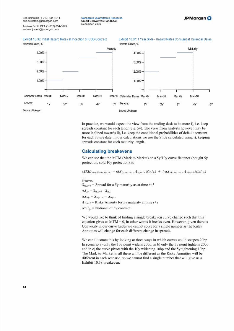
5/10/2018 JPM Credit Derivatives - slidepdf.com
http://slidepdf.com/reader/full/jpm-credit-derivatives-559e0102dc371 84/180
Eric Beinstein (1-212) [email protected]
Andrew Scott, CFA (1-212) [email protected]
Corporate Quantitative ResearchCredit Derivatives HandbookDecember, 2006
84
Exhibit 10.36: Initial Hazard Rates at Inception of CDS Contract
Hazard Rates, %
Mar-06 Mar-07 Mar-08 Mar-09 Mar-10
1.00%
2.00%
3.00%
4.00%
1Y 2Y 3Y 4Y 5Y
Calendar Dates:
Tenors:
Maturity
Source: JPMorgan
Exhibit 10.37: 1 Year Slide - Hazard Rates Constant at Calendar Dates
Hazard Rates, %
Mar -07 Mar -08 Mar -09 Mar -10
1.00%
2.00%
3.00%
4.00%
1Y 2Y 3Y 4Y 5Y
Calendar Dates:
Tenors:
Maturity
Source: JPMorgan
In practice, we would expect the view from the trading desk to be more i), i.e. keep
spreads constant for each tenor (e.g. 5y). The view from analysts however may be
more inclined towards ii), i.e. keep the conditional probabilities of default constant
for each future date. In our calculations we use the Slide calculated using i), keeping
spreads constant for each maturity length.
Calculating breakevens
We can see that the MTM (Mark to Market) on a 5y/10y curve flattener (bought 5y
protection, sold 10y protection) is:
MTM Curve Trade, t to t+1 = ( ∆S 5y, t to t+1 . A5y,t+1 . Ntnl 5y ) + (- ∆S 10y, t to t+1 . A10y,t+1.Ntnl 10y )
Where,S 5y, t+1 = Spread for a 5y maturity as at time t+1
∆S 5y = S 5y, t+1 - S 5y, t
∆S 10y = S 10y, t+1 – S 10y, t
A5y,t+1 = Risky Annuity for 5y maturity at time t+1
Ntnl 5y = Notional of 5y contract.
We would like to think of finding a single breakeven curve change such that this
equation gives us MTM = 0, in other words it breaks even. However, given there is
Convexity in our curve trades we cannot solve for a single number as the Risky
Annuities will change for each different change in spreads.
We can illustrate this by looking at three ways in which curves could steepen 20bp.
In scenario a) only the 10y point widens 20bp, in b) only the 5y point tightens 20bp
and in c) the curve pivots with the 10y widening 10bp and the 5y tightening 10bp.
The Mark-to-Market in all these will be different as the Risky Annuities will be
different in each scenario, so we cannot find a single number that will give us a
Exhibit 10.38 breakeven.

5/10/2018 JPM Credit Derivatives - slidepdf.com
http://slidepdf.com/reader/full/jpm-credit-derivatives-559e0102dc371 85/180
Eric Beinstein (1-212) [email protected]
Andrew Scott, CFA (1-212) [email protected]
Corporate Quantitative ResearchCredit Derivatives HandbookDecember, 2006
85
Exhibit 10.38: Illustration of a 20bp Curve Steepening Causing Different Mark to Marketsbp
a) Curve Steepening 20bp by 10y
only widening
0
20
40
60
80100
0 2 4 6 8 10
Start, t
End, t+1
b) Curve Steepening 20bp by 5y
only tightening
0
20
40
60
80
0 2 4 6 8 10
Start, t
End, t+1
c) Curve Steepening 20bp: 10y
widening 10bp & 5y tightening 10bp
0
20
40
60
80
100
0 2 4 6 8 10
Start, t
End, t+1
Source: JPMorgan
In practice, we therefore analyse Breakevens by looking at discrete changes in a
given point (say the shorter maturity leg for ease sake) and then calculate at howmuch the longer maturity leg needs to move such that our trade MTM = 0.
We can therefore define Breakeven Curve t+1 | S n, t+1 = S’ as the breakeven Curve at
time t+1 conditional on the Spread at the n year point at t+1 being S’ . For example,
if the 5y point (S 5, t+1,) is at 50bp (S’ ) at the trade horizon t+1, where does the Curve
need to be so that the 10y point ensures that the MTM = 0 for a 5y / 10y curve trade.
We can show these Breakevens as a range around the current spread as in Exhibit
10.39. The Breakeven for Time is the highlighted row where the 5y point is
unchanged over the horizon. The other rows represent Breakevens for a Given 5y
Spread Change. We change the 5y spread to see how far the curve has to steepen or
flatten at the 10y point for the trade to breakeven given the 5y Spread change and the
effect of Time. The real Breakeven needs to show how much the curve needs to
flatten or steepen versus the Slide Implied Curve (this is shown in the final column)as the Slide will imply a natural curve move over the life of the trade.
Exhibit 10.39: Breakeven Curve Movements Analysi s
5y/10y Curve Movement (in bp) Needed to Breakeven With a Duration-Weighted Flattener Over 3 Months
Chg in 5y 5Y (Slide Implied) 10Y Breakeven Breakeven Curve (10Y-5Y) Breakeven Curve Chg Breakeven Curve Chg(vs Slide Implied) bp bp bp bp (vs current curve) bp (vs Slide implied) bp
-40 296 339 43.4 -5.9 -23.1-20 316 357 41.2 -8.1 -25.2
0 336 375 39.3 -10.0 -27.220 356 393 37.6 -11.7 -28.940 376 412 36.0 -13.3 -30.4
Source: JPMorgan

5/10/2018 JPM Credit Derivatives - slidepdf.com
http://slidepdf.com/reader/full/jpm-credit-derivatives-559e0102dc371 86/180
Eric Beinstein (1-212) [email protected]
Andrew Scott, CFA (1-212) [email protected]
Corporate Quantitative ResearchCredit Derivatives HandbookDecember, 2006
86
The Horizon Effect
Sensitivity analysis of curve trades at their horizon can be a complex issue. Here we
examine the Horizon Effect on curve trades, which we define as the impact of the
trade horizon on a trade’s sensitivity to parallel spread changes.
The Horizon Effect can be most easily seen by the difference in our sensitivity
analysis for a Duration-Weighted trade between instantaneous changes in spread and
changes in spread at horizon. The reason we have a Horizon Effect is because our
Risky Annuities change over the life of a trade. This causes a Duration-Weighted
trade – which is intended to be neutral to directional (parallel) spread moves – to
become longer or shorter spread risk over the life of the trade. In other words, the
change in Risky Annuities (and Durations) causes the trade to be un-Duration-
Weighted over the trade horizon. So why do Risky Annuities change over the life of
a curve trade?
Changing Risky Annuities over the Trade Horizon
There are two effects that cause Risky Annuities change over a trade horizon, if the
curve itself is unchanged:
a) Impact of maturity decreasing
As the length of time to maturity decreases, Risky Annuities fall and shorter-dated
Risky Annuities fall more than longer-dated Risky Annuities. For example, the effect
of 6 months of time passing could make the 10y Risky Annuity decrease from 8.50
to 8.25 and the 5y decrease from 4.50 to 4.00. This is easiest to illustrate by picturing
a flat curve as shown in Exhibit 10.40, where only the effect of time passing changes
the Risky Annuities.
As our shorter leg Risky Annuity declines faster, we will no longer be Duration-
Weighted. Essentially we will be getting longer risk in a Flattener, as we will nothave enough protection in our short risk leg of the trade at horizon to be Duration-
Weighted.
b) Roll Down / slide effect
Given that credit curves are typically upward sloping and often steeper at the short
end than at the long end, the roll-down or Slide effect typically has the effect of a
non-parallel tightening of a curve trade, as shown in Exhibit 10.41.
Spread tightening will mean that Risky Annuities rise in both legs.
We call the net effect of both of these factors on Risky Annuities changing over time
the Horizon Effect. The net effect will depend on the shape of the particular curve
and time horizon, but for normal shaped curves (e.g. our previous example of FiatSPA) and for 5y/10y trades, maturity effect will tend to dominate the roll down
effect.
A worked example
A real-life example will help to show how the Horizon Effect of changing Risky
Annuities affects the directional position of a trade. We will look at a our example
from the main body of the note, a Duration-Weighted curve flattener on Fiat SPA
where we buy protection in 5y and sell protection in 10y Duration-Weighted (as
shown in Exhibi VII.3). We analyse this curve trade for a 6 month horizon. The
curve for Fiat SPA is shown in Exhibit 10.43.
Exhibit 10.40: Maturity EffectFlat Spread Curve (x-axis: Maturity, years; y-axis:
Spread, bp)
0
20
40
60
80
100
0 1 2 3 4 5 6 7 8 9 10
Original Curve
Source: JPMorgan
Exhibit 10.41: Roll / Slide Effect (bp)x-axis: Maturity, years; y-axis: Spread, bp
020
40
60
80
100
120
0 1 2 3 4 5 6 7 8 9 10
9.5y Spread
10y Spread
5y Spread
4.5y Spread
Source: JPMorgan

5/10/2018 JPM Credit Derivatives - slidepdf.com
http://slidepdf.com/reader/full/jpm-credit-derivatives-559e0102dc371 87/180
Eric Beinstein (1-212) [email protected]
Andrew Scott, CFA (1-212) [email protected]
Corporate Quantitative ResearchCredit Derivatives HandbookDecember, 2006
87
Exhibit 10.42: Worked Convexity Exampl e – Duration-Weighted Flattener on Fiat SPA
Spread Notion al ($) RiskyTenor Position bp (Default Exposure) Annuity5Y Buy Protection 355 -15,520,593 4.2510Y Sell Protection 404 +10,000,000 6.59
Source: JPMorgan
Instantaneous parallel spread moves
If the curve moves parallel wider or tighter, Risky Annuities change in our Duration-
Weighted trade giving us a Convexity impact (as shown in Exhibit 10.44). As we
have seen, a Flattener has a Positive Convexity meaning it has a positive MTM effect
from both a tightening and widening of spreads.
Exhibit 10.43: Fiat SPA Credit Curve
x-axis: Maturity in years; y-axis: Spread, bp
355
404
0
100
200
300
400
500
0 1 2 3 4 5 6 7 8 9 10
Source: JPMorgan
Exhibit 10.44: Convexity Effect for (Instantaneous) 20bp ParallelCurve Shifts
x-axis: parallel curve move in bp; y-axis: MTM ($)
0
1,000
2,000
3,000
4,000
-40 -20 0 20 40
Source: JPMorgan
Horizon Effect on Risky AnnuitiesAs the trade Slides over the trade horizon we will get both a shortening of maturity
and a non-parallel tightening of spreads. We can see this effect in Exhibit 10.45
where we have the maturity declining 6 months and the spreads tightening from
355bp to 336bp in the 5y leg of the trade and from 404bp to 402bp in the 10y leg of
the trade.
Exhibit 10.45: Slide Impact on Spread and Maturity
bp
355404
0
100
200
300
400
500
0 1 2 3 4 5 6 7 8 9 10
336402
Source: JPMorgan
Positive Convexity from Parallel
Spread Moves in Isolation

5/10/2018 JPM Credit Derivatives - slidepdf.com
http://slidepdf.com/reader/full/jpm-credit-derivatives-559e0102dc371 88/180
Eric Beinstein (1-212) [email protected]
Andrew Scott, CFA (1-212) [email protected]
Corporate Quantitative ResearchCredit Derivatives HandbookDecember, 2006
88
The roll (tightening) effect should make Risky Annuities rise and the Maturity effect
will mean that Risky Annuities will fall, with the 5y Risky Annuity falling more than
the 10y. The net results of these different Slide effects will differ case by case.
In our example, where the trade horizon is 6 months, the 5y Risky Annuity ends upmoving from 4.25 to 3.92 (-0.33) and the 10y Risky Annuity ends up moving from
6.59 to 6.42 (-0.17), i.e. our 5y Risky Annuity falls more than our 10y. This makes our
trade longer risk over the horizon. Exhibit 10.46 shows how we work through this. We
look at the current Duration-Weighting (column 6) and then using our Slide Implied
horizon Risky Annuities look at how we should be Duration-Weighting at horizon,
assuming the curve is unchanged. The difference can be seen in the final column, the
Horizon Effect. We can see that as our 5y Risky Annuity falls more, we should be
buying more protection (shorter risk) at horizon. I.e. to be Duration-Weighted at
horizon we need to have bought protection on $16,373,090 but we have only bought
protection on $15,520,593. Essentially, we are less short than we should be in the 5y
leg (+$852,498), so we have become longer risk over the life of the trade.
Exhibit 10.46: Change in Annu ities and Horizon Effect
Current Spread(bp)
Slide ImpliedSpread (bp)
Current Annuity
Slide Implied Annuity
Current Duration-Weighting
Horizon Duration-Weighting
HorizonEffect
Buy 5Y 355 336 4.25 3.92 -15,520,593 -16,373,090 +852,498Sell 10Y 404 402 6.59 6.42 +10,000,000 +10,000,000 0Curve 49 66
Source: JPMorgan
Isolating the Horizon Effect
We can see the impact of this Horizon Effect when we look at sensitivity analysis at
horizon. Exhibit 10.47 shows the MTM of the trade at horizon including the Slide,
which shows the large negative Slide effect (-$102,394) in this trade dominates
horizon P+L if curves are unchanged. When we take out the Slide effect in Exhibit
10.48 we can see the Horizon Effect as we are now long risk, so that a widening of
spreads has a MTM loss and a tightening of spreads has a MTM gain. CompareExhibit 10.48 to Exhibit 10.44 to see how we get a very different pattern for a change
in spreads at the start of the trade and at its horizon.
Exhibit 10.47: Sensitivity Analysis at Horizon Including Slide
x-axis: Spread Change at Horizon (bp), y-axis: Trade MTM ($)
-120,000
-100,000
-80,000
-60,000
-40,000
-20,000
0
-40 -20 0 20 40
Source: JPMorgan
Exhibit 10.48: Sensitivity Analysis at Horizon minus Slide
x-axis: Spread Change at Horizon (bp), y-axis: MTM ($)
-15,000
-10,000
-5,000
0
5,000
10,000
15,000
20,000
-40 -30 -20 -10 0 10 20 30 40
MTM At Horizon (minus Slide)
incl. Convexity
Pure Horizon Effect
Source: JPMorgan
We summarize this horizon effect by looking at how the trade MTM at horizon (less
Slide) differs from the instantaneous MTM for changes in spread, as we see in the

5/10/2018 JPM Credit Derivatives - slidepdf.com
http://slidepdf.com/reader/full/jpm-credit-derivatives-559e0102dc371 89/180
Eric Beinstein (1-212) [email protected]
Andrew Scott, CFA (1-212) [email protected]
Corporate Quantitative ResearchCredit Derivatives HandbookDecember, 2006
89
final row of Exhibit 10.49. The trade is now longer risk and so has a more negative
MTM as spread widen and a less negative MTM as spreads tighten.
Exhibit 10.49: Sensitivity Analysis at Horizon
MTM from Given Spread Changes ($)-40bp Spread Chg -20bp Spread Chg 0bp Spread Chg 20bp Spread Chg 40bp Spread Chg
1) MTM 5Y (Buy) -362,295 -238,680 -117,054 3,264 121,6452) MTM 10Y (Sell) 275,938 143,497 14,660 -110,704 -232,6723) Curve Trade MTM at Horizon -86,357 -95,183 -102,394 -107,440 -111,0264) Curve Trade MTM at Horizon minus Slide 16,037 7,211 0 -5,045 -8,6325) Instantaneous MTM 3,452 849 0 821 3,2326) Horizon Effect (Row 4 – Row 5) 12,585 6,363 0 -5,867 -11,864
Source: JPMorgan
Horizon Effect Conclusion
The Horizon Effect gives us a market directional position over the life of the trade
due to our changing Risky Annuities. This can affect our sensitivity analysis for
spread changes at the horizon. The net risk position we pick-up in a trade is difficult
to predict with certainty and will depend on:
The shape of the underlying curve
The time between the maturities of the trade
The length of the horizon we are considering
We can remove the Horizon Effect in a curve trade by Forward Duration-Weightingthe trade so that it is weighted to be market-neutral at horizon, given the Slide-implied Risky Durations. This weighting would need to be continually adjusted asany curve movements would change our Forward Durations. Practically, manytraders will Duration-Weight their curve trades for the current Durations, but should be aware of how the Horizon Effect will give them a longer or shorter risk positionover the life of the trade.
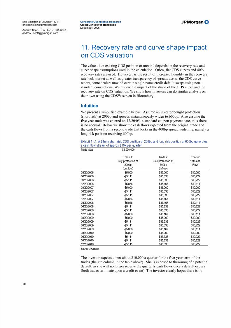
5/10/2018 JPM Credit Derivatives - slidepdf.com
http://slidepdf.com/reader/full/jpm-credit-derivatives-559e0102dc371 90/180
Eric Beinstein (1-212) [email protected]
Andrew Scott, CFA (1-212) [email protected]
Corporate Quantitative ResearchCredit Derivatives HandbookDecember, 2006
90
11. Recovery rate and curve shape impact
on CDS valuationThe value of an existing CDS position or unwind depends on the recovery rate andcurve shape assumptions used in the calculation. Often, flat CDS curves and 40%recovery rates are used. However, as the result of increased liquidity in the recoveryrate lock market as well as greater transparency of spreads across the CDS curvetenors, some dealers unwind certain single-name credit default swaps using non-standard conventions. We review the impact of the shape of the CDS curve and therecovery rate on CDS valuation. We show how investors can do similar analysis ontheir own using the CDSW screen in Bloomberg.
Intuition
We present a simplified example below. Assume an investor bought protection(short risk) at 200bp and spreads instantaneously widen to 600bp. Also assume thefive year trade was entered on 12/20/05, a standard coupon payment date, thus thereis no accrual. Below we show the cash flows expected from the original trade andthe cash flows from a second trade that locks in the 400bp spread widening, namely along risk position receiving 600bp.
Exhibit 11.1: A $1mm short risk CDS position at 200bp and long risk position at 600bp generatesa cash flow stream of appro x $10k per quarter Trade Size $1,000,000
Trade 1: Trade 2: Expected
Buy protection at Sell protection at Net Cash
200bp 600bp Flow
(outflow) (inflow)
03/20/2006 -$5,000 $15,000 $10,000
06/20/2006 -$5,111 $15,333 $10,222
09/20/2006 -$5,111 $15,333 $10,222
12/20/2006 -$5,056 $15,167 $10,111
03/20/2007 -$5,000 $15,000 $10,000
06/20/2007 -$5,111 $15,333 $10,222
09/20/2007 -$5,111 $15,333 $10,222
12/20/2007 -$5,056 $15,167 $10,111
03/20/2008 -$5,056 $15,167 $10,111
06/20/2008 -$5,111 $15,333 $10,222
09/20/2008 -$5,111 $15,333 $10,222
12/20/2008 -$5,056 $15,167 $10,111
03/20/2009 -$5,000 $15,000 $10,000
06/20/2009 -$5,111 $15,333 $10,222
09/20/2009 -$5,111 $15,333 $10,222
12/20/2009 -$5,056 $15,167 $10,11103/20/2010 -$5,000 $15,000 $10,000
06/20/2010 -$5,111 $15,333 $10,222
09/20/2010 -$5,111 $15,333 $10,222
12/20/2010 -$5,111 $15,333 $10,222
Source: JPMorgan
The investor expects to net about $10,000 a quarter for the five-year term of thetrades (the 4th column in the table above). She is exposed to the timing of a potentialdefault, as she will no longer receive the quarterly cash flows once a default occurs(both trades terminate upon a credit event). The investor clearly hopes there is no

5/10/2018 JPM Credit Derivatives - slidepdf.com
http://slidepdf.com/reader/full/jpm-credit-derivatives-559e0102dc371 91/180
Eric Beinstein (1-212) [email protected]
Andrew Scott, CFA (1-212) [email protected]
Corporate Quantitative ResearchCredit Derivatives HandbookDecember, 2006
91
default at all; or, if there is one, that it is as far in the future as possible so that shecontinues to receive the positive cash flow stream.
In the event of default, the investor is insensitive to recovery rate as the two tradesare offsetting. Specifically, on the short protection position she will receive a bondwhich she can deliver to settle the long protection position. Furthermore, she may beable to use a CDS settlement protocol, detailed in Part I, and settle both trades at thesame recovery rate.
Alternatively, and more commonly, the investor will seek to unwind the first trade,receiving the present value of the quarterly cash flows as a single payment today. Asdiscussed in Part I, to value CDS we discount cash flows using swap curve baseddiscount factors, and probability of default discount factors. In essence, we find the present value of the $10k quarterly cash flows, multiplied by the probability that thecash flows are paid, or one minus the probability the credit defaults. The CDSspreads and recovery rates used to calculate these probabilities effect the value of theCDS contract.
CDS curve shape impact
The curve shape assumption affects the assumed timing of default, or the probabilityof default in a given year. Consider scenarios A and B. In scenario A, there is a 50%chance of a default tomorrow and a 50% chance the credit does not default during thefive year life of the contract. In scenario B, there is a 50% chance of a default in 4.75years (thus receiving all but one quarterly payment), and a 50% chance the creditdoes not default. The risky present value of the cash flows is higher in scenario Bthan in A. Scenario A is more like a flat curve, with large probabilities of default inthe early years of the contract. Scenario B is more like a steep curve, with small probabilities of default in the early years and larger probabilities in the later years.
Another way to think about the curve shape impact on the mark-to-market of CDS is
using the concept of duration. Duration is often thought of as the weighted averageterm to maturity of cash flows. Steeper curves exhibit higher duration than flatter curves as lower spreads at the front end imply lower probability of default early inthe life of the trade and higher spreads at the backend imply higher default probability later in the life of the trade. A higher duration therefore implies that wereceive cash flows for a longer period of time, thus the value of our CDS contractshould be higher.
Below we show two curves, each with 5Y CDS equal to 500bp. The steeper curvehas a longer duration. The present value of a CDS contract is equal to the change inspread multiplied by the risky duration. Thus, the greater the duration the larger the present value.

5/10/2018 JPM Credit Derivatives - slidepdf.com
http://slidepdf.com/reader/full/jpm-credit-derivatives-559e0102dc371 92/180
Eric Beinstein (1-212) [email protected]
Andrew Scott, CFA (1-212) [email protected]
Corporate Quantitative ResearchCredit Derivatives HandbookDecember, 2006
92
Exhibit 11.2:Flat and Steep Curve with same 5Y Spread
duration = 3.43
duration = 3.63
500bp
0
200
400
600
800
1000
1200
1y 2y 3y 4y 5y 6y 7y 8y 9y 10y
bp
Flat Curve Steep Curve
Source: JPMorgan
Recovery rate impact
The recovery rate’s impact on CDS valuation is more subtle. Recovery rates effectdefault probabilities, and thus effect the valuation of cash flows. Consider thefollowing equation:
CDS spread ≈ (1-Recovery) x Probability of default
In other words, CDS spreads are equal to the potential loss in default multiplied bythe probability of default. Re-arranging the terms gives
Probability of default ≈ CDS spread / (1 – Recovery)
Therefore, for a given CDS spread, the higher the recovery rate assumption thehigher the default probability assumed. The investor in our example wants a lowdefault probability so that the present value of the cash flow stream is higher. Thus,she wants a low assumed recovery rate.
In this table we show the MTM (in $000’s) of a 5Y CDS entered at 300bp andunwound at a flat spread specified in the column using different recoveryassumptions.
Exhibit 11.3: CDS MTM for un wind of $10MM 5Y short risk p ositio n on 12/9/2005, entered at 300bpUnwind Spread ($000s)
Unwind Recovery 100bp 300bp 500bp
50% -$858 $0 $71440% -$865 $0 $74130% -$870 $0 $761
Source: JPMorgan.
Note that the difference in MTM of the unwind between the 30% and 50% recoveryassumptions is greater when unwinding at 500bps ($761 - $714 = $47) than whenunwinding at 100bps ($870 - $858 = $12). This is logical as CDS MTM is moresensitive to recovery rate at wider spread levels since the credit is closer to defaultand recovery rates are closer to being realized. We can see this graphically in theslope of the curve below. It plots P/L on the unwind (Y-Axis) against recovery rate(X-Axis). As recovery rates increase the curve becomes steeper. Intuitively, ahigher recovery leads to higher default probability, which means that one is more

5/10/2018 JPM Credit Derivatives - slidepdf.com
http://slidepdf.com/reader/full/jpm-credit-derivatives-559e0102dc371 93/180
Eric Beinstein (1-212) [email protected]
Andrew Scott, CFA (1-212) [email protected]
Corporate Quantitative ResearchCredit Derivatives HandbookDecember, 2006
93
likely to experience and settle at that recovery. CDS MTM is also more sensitive torecovery at higher spreads for the same reason.
Exhibit 11.4: MTM of lon g prot ection 5y CDS entered at 300bp unwo und at 500bp.
CDS MTM (000's) vs Recovery Rate Assumpti on
$0
$100
$200
$300
$400
$500
$600
$700
$800
$900
10% 20% 30% 40% 50% 60% 70% 80% 90% 95%
Note: in $000’sSource: JPMorgan
Assumptions at contract inception
When one enters a standard CDS trade (as opposed to a fixed recovery CDS trade)there is no explicit or implied recovery rate or curve shape assumption. Two parties
are simply agreeing on a spread to exchange. When one party agrees to buy protection from another at 200bps, for example, she may have very different viewsfrom the seller on the recovery rate that will prevail should there be a default in thefuture. This is irrelevant in the trade, thus, there is no concept of recovery rate“changing” between the original trade and the unwind.
Since different dealers may use different conventions, investors must know theunwind assumptions (curve shape and recovery) corresponding to a spread tounderstand the economic impact. For example, an investor who bought protectionand wants to unwind the contract may typically look for the highest bid. This isreasonable if the conventions used in the quotes are the same. If they are not,however, an investor may be better off unwinding at a lower bid if the conventionsused are more in his favor (steeper curve and/or lower recovery / lower default probability).
To summarize, for an investor who bought protection at 200bps and is unwinding at600bps:
Higher recovery (higher default probability) leads to lower absolute MTM on theunwind
Steeper CDS curve (default not likely to happen until later in the trade) leads tohigher absolute MTM on a CDS contract
For an investor who sold protection and is unwinding at a higher spread (for a loss)the opposite is true.

5/10/2018 JPM Credit Derivatives - slidepdf.com
http://slidepdf.com/reader/full/jpm-credit-derivatives-559e0102dc371 94/180
Eric Beinstein (1-212) [email protected]
Andrew Scott, CFA (1-212) [email protected]
Corporate Quantitative ResearchCredit Derivatives HandbookDecember, 2006
94
Worked examples
Assume an investor entered in a five-year contract buying protection at 200bps witha trade size of $1mm. If the current 5Y spread remains at 200bps, the CDS marketvalue is zero regardless of the recovery rate (Exhibit 11.5) and the curve shape(Exhibit 11.6).
Exhibit 11.5
Source: Bloomberg
Exhibit 11.6
Source: Bloomberg
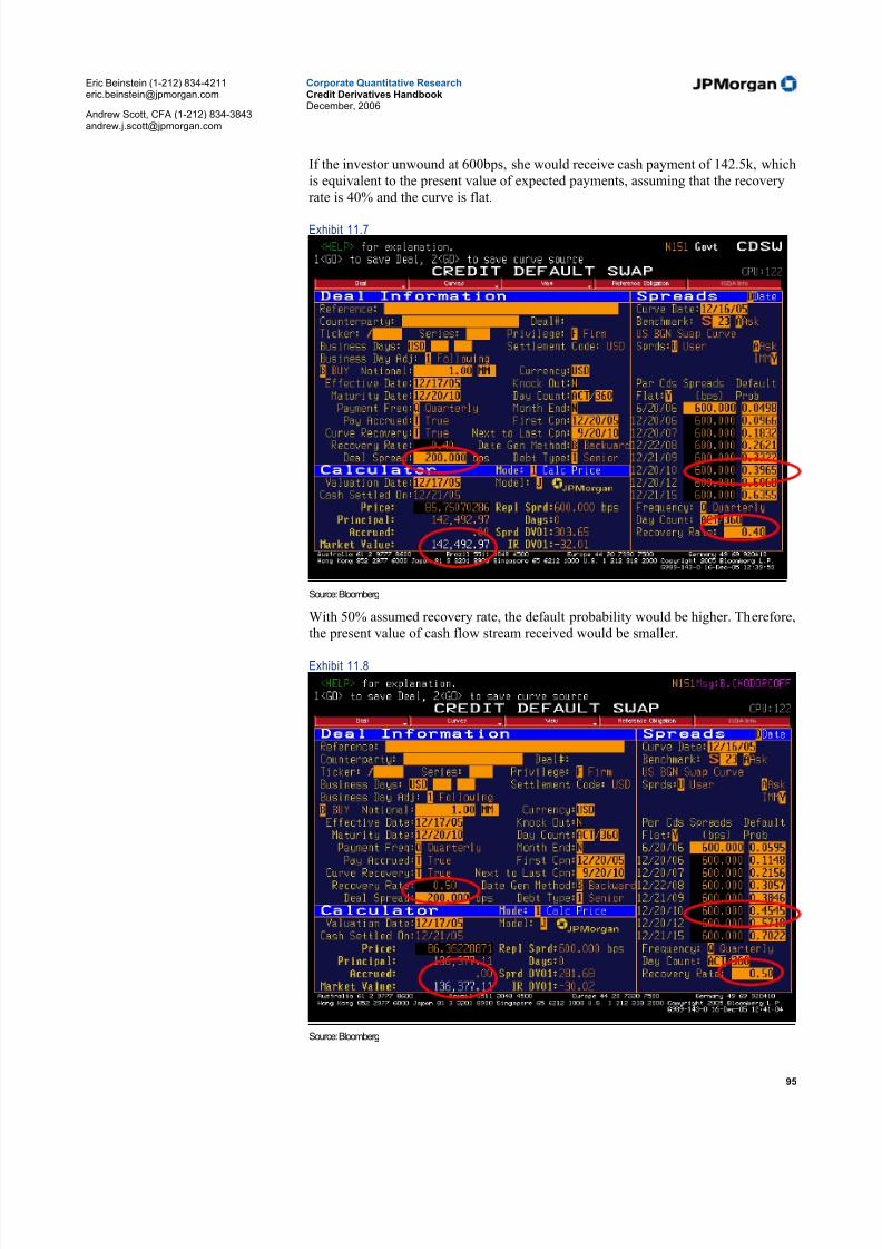
5/10/2018 JPM Credit Derivatives - slidepdf.com
http://slidepdf.com/reader/full/jpm-credit-derivatives-559e0102dc371 95/180
Eric Beinstein (1-212) [email protected]
Andrew Scott, CFA (1-212) [email protected]
Corporate Quantitative ResearchCredit Derivatives HandbookDecember, 2006
95
If the investor unwound at 600bps, she would receive cash payment of 142.5k, whichis equivalent to the present value of expected payments, assuming that the recoveryrate is 40% and the curve is flat.
Exhibit 11.7
Source: Bloomberg
With 50% assumed recovery rate, the default probability would be higher. Therefore,the present value of cash flow stream received would be smaller.
Exhibit 11.8
Source: Bloomberg
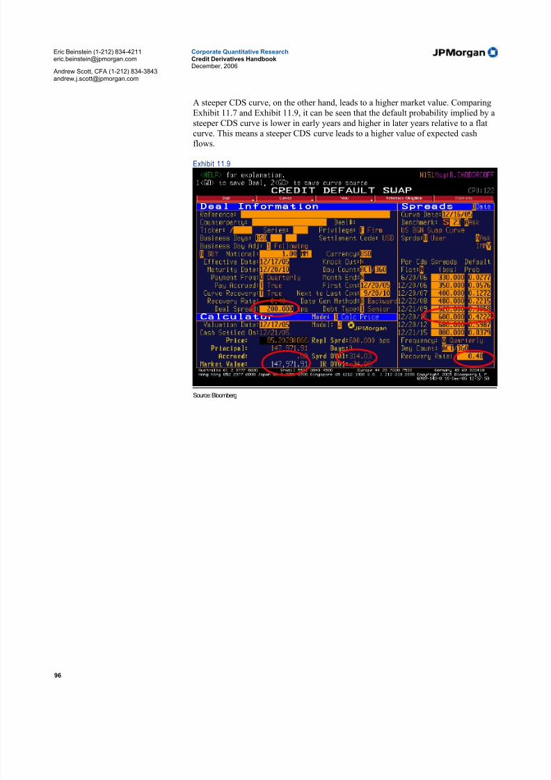
5/10/2018 JPM Credit Derivatives - slidepdf.com
http://slidepdf.com/reader/full/jpm-credit-derivatives-559e0102dc371 96/180
Eric Beinstein (1-212) [email protected]
Andrew Scott, CFA (1-212) [email protected]
Corporate Quantitative ResearchCredit Derivatives HandbookDecember, 2006
96
A steeper CDS curve, on the other hand, leads to a higher market value. ComparingExhibit 11.7 and Exhibit 11.9, it can be seen that the default probability implied by asteeper CDS curve is lower in early years and higher in later years relative to a flat
curve. This means a steeper CDS curve leads to a higher value of expected cashflows.
Exhibit 11.9
Source: Bloomberg

5/10/2018 JPM Credit Derivatives - slidepdf.com
http://slidepdf.com/reader/full/jpm-credit-derivatives-559e0102dc371 97/180
Eric Beinstein (1-212) [email protected]
Andrew Scott, CFA (1-212) [email protected]
Corporate Quantitative ResearchCredit Derivatives HandbookDecember, 2006
97
12. Trading credit versus equity
Equity, Equity Option and Credit Derivative markets are all deep, liquid markets,where company news, macro events, and market flows are quickly reflected in pricesand spreads. When bad news occurs, for example, equity prices usually fall, creditspreads rise, and equity option implied volatility usually increases. However, evenwhen markets move in the expected direction, the extent of the moves may be verydifferent. For example, if a stock price falls from $20 to $19, credit spreads rise from100bp to 120bp, and equity volatility rises from 35% to 40%, it is not obviouswhether each of these moves is “reasonable” relative to the others.
One approach is to use historical relationships between the markets to determinewhat is “reasonable.” This method does not determine if market pricing betweenassets is “correct,” as this is a subjective assessment requiring an understanding of the company and market environment. Rather, it simply identifies where
relationships have changed. Investors can then determine whether the cross-assetrelationship breakdown is justifiable or if there is a trade opportunity.
We discuss four market variables that can be used to track firm-specific performanceand identify potential pricing discrepancies:
• Equity price
• Five-year credit default swap spread
• Implied volatility of six-month at-the-money equity options
• The 90-100% six-month equity volatility skew—this is the difference between implied volatility of options struck at 90% of the at-the-moneystrike and implied volatility of at-the-money options
Relationships in equity and credit markets
We analyze four different relationships between market variables of the same firm.
Equity price versus five-year CDS spread Typically, these two market variables are inversely related. That is, when a firm’sstock is increasing, CDS spreads are usually tightening. We say “usually” becauseoccasionally there is justification for stock and CDS spreads to move in the samedirection. A typical example is a leveraged buyout, which often leads to an increasein a firm’s stock price and widening of the CDS spreads.
The five-year CDS spread is used as the benchmark credit market price, rather than a bond spread. This is because five-year CDS spreads are standardized. In other words,if company A has a five-year CDS spread of 200bp and company B has a five-year
CDS spread of 150bp, it is fair to conclude that company A is being priced by themarket as 50bp wider. One could not do a similar comparison with bonds becausecompanies issue bonds with different coupons and maturities. These characteristicshave to be normalized before making comparisons.
Equity price versus six-month at-the-money implied volatilityStock price and implied volatility of options on the same stock tend to be inverselyrelated. Volatility increases as the stock price falls and decreases as the stock pricerises. The standard explanation for this relationship is the so-called "leverage effect."The fall in stock leads to an increase in the firm’s leverage, meaning the risk to both bondholders and stockholders increases. As equity risk increases, return volatilityincreases as well.

5/10/2018 JPM Credit Derivatives - slidepdf.com
http://slidepdf.com/reader/full/jpm-credit-derivatives-559e0102dc371 98/180
Eric Beinstein (1-212) [email protected]
Andrew Scott, CFA (1-212) [email protected]
Corporate Quantitative ResearchCredit Derivatives HandbookDecember, 2006
98
Five-year CDS spread versus six-month at-the-money implied volatility
Implied volatility of options on a firm’s stock is the market’s forecast of future
volatility. Since volatility can be viewed as a measure of a firm’s riskiness, it can bedirectly related to CDS spread, which is also a measure of risk. Therefore, as a firm’simplied volatility increases, one would expect CDS spreads to widen. This istypically what is observed in the market.
Five-year CDS spread versus 90-100% six-month at-the-money implied volatility skewOption prices are often expressed in terms of their implied volatilities. One mightexpect that all options on the same underlying would trade at the same level of implied volatility. This is almost never the case, however. A plot of impliedvolatilities of equity options across different strikes typically looks like a downwardsloping line. This relationship implies that options at lower strikes (say, at 90% of thecurrent stock price) are relatively more expensive than options at higher strikes (say,at 110% of the current stock price). This may suggest that the market believes there
is greater chance of the stock price falling than is assumed by the lognormaldistribution property of the Black-Scholes model. The skew, as it is defined in thisreport (implied volatility of options struck at 90% of the at-the-money strike less theimplied volatility of option struck at-the-money) is a measure of the higher cost of out-of-the-money puts, which are often bought to protect against a large downwardmove in the stock. An increase in the skew suggests that the market considers a largedownward move more likely. If the credit market shares this belief, the CDS spreadsare likely to widen as well. This relationship suggests that there is a positivecorrelation between implied volatility skew and CDS spreads.
Finding trade ideas
We can look for trade ideas by observing historical relationships and noting whenrelative pricing patterns change. In this example we consider the behavior of General
Motors Corporation’s stock and five-year CDS spreads in April through June 2005.Below are one-year charts of General Motors’ stock price and five-year CDS.
Source: JPMorgan
Stock reaches low on 15-Apr-2005 at $25.60
CDS reaches widest spread level one
month later on 17-May-2005 at 1091bp.

5/10/2018 JPM Credit Derivatives - slidepdf.com
http://slidepdf.com/reader/full/jpm-credit-derivatives-559e0102dc371 99/180
Eric Beinstein (1-212) [email protected]
Andrew Scott, CFA (1-212) [email protected]
Corporate Quantitative ResearchCredit Derivatives HandbookDecember, 2006
99
The fact that the widest CDS spread was observed a month after the lowest equity price suggests that during this highly volatile period for General Motors, the equityand CDS markets were not operating in sync. Whenever this happens (i.e., whenever
the two markets diverge), a convergence trade may be attractive. This trade isessentially a view on a reestablishment of the historical relationship between the twomarkets. In this case, the position on May 17 would be that the CDS and equity pricewill converge, i.e. the CDS market is too bearish and spreads would tighten to comemore in line with the stock price; OR, the equity market is too bullish and the stock price would drop to be more in line with the CDS spread. Given this view, a potentialtrade would be to sell CDS protection (go long credit risk) and short the stock.
Judging a potential mis-pricing between two markets is not very easy from the timeseries charts. This is why we include regression charts on the same page of our daily“Cross Asset Class Relative Performance” report. These charts quantify whether thecurrent pricing in the two markets is out of line with the historical pattern.
Below is a chart of the one-year regression between the stock price and CDS on May17, 2005. The larger circles correspond to more recent data on May 17, with the black dot representing the most recent observation. The Z-Score output of the regressionmodel specifies how far out of line the most recent observation is with respect to theone-year historical relationship. A Z-Score of zero means the current observation isidentical to the value predicted by the model. A Z-Score of less than -2 or greater than2 means there is significant deviation from the historical relationship. The two greycurves are two-standard deviation confidence interval bands. Approximately 95% of variation lies between these bands. R 2 ranges from 0% to 100% and captures thestrength of the relationship, with 100% being a perfectly correlated relationship. In our case, a relatively high R 2 of 85% between the stock and CDS means the two havemoved very much in line in the past year. A Z-Score of 3.2 means there is a verysignificant deviation from this historically strong relationship. Below is an exhibit fromour Cross Asset Class Relative Performance Report, which compares General MotorsCorp (GM) stock prices (y-axis) to CDS spread (x-axis).
Source: JPMorgan
Black dot shows stock pric(y-axis) and five-year CDSspread (x-axis) on May 172005. Pricing is well outsithe historically predicted
A high R-Sq indicates that theCDS–Equity relationship has been strong historically.
A Z-Score of 3.2 ishighly significant,indicating a large pricing discrepancy.
The model-predicted stock price (plotted on the y-axis) is$24.09, which is $6.76 lower than the market price of $30.85. In other words, giventhe current CDS level, thehistorically predicted equity price is $24.09.
For the current equity price,the historically predicted levelof CDS is 583bp.

5/10/2018 JPM Credit Derivatives - slidepdf.com
http://slidepdf.com/reader/full/jpm-credit-derivatives-559e0102dc371 100/180
Eric Beinstein (1-212) [email protected]
Andrew Scott, CFA (1-212) [email protected]
Corporate Quantitative ResearchCredit Derivatives HandbookDecember, 2006
100
Below is the same chart plotted two weeks later, on June 3, 2005. In the two weeksfollowing the observation above, the CDS tightened 370bp, while the stock went up$0.08. The Z-Score fell to 0.5, indicating the relationship between the stock and CDS
has been re-established. The black dot is closer to the black line, its predicted level.The convergence trade would have lost $0.08 on the short stock position but gained370bp on the CDS leg.
The slope in the regression output above tells us that for each 1bp increase in theCDS spread, the stock is expected to fall by approximately $0.01. Given a notionalon the CDS, we can use this relationship to find the number of shares to trade. Usingthe Bloomberg CDSW tool, for a given CDS contract, we can find the Spread DV01,or the P/L due to the 1bp move in CDS. Once we know this dollar amount, and givenan expected $0.01 drop in share, we can determine how many shares to trade to giveus approximately the reverse P/L on the equity leg, assuming the historicalrelationship holds.
Source: JPMorgan
A worked trade recommendation
When we recommend CDS versus stock strategies, we often combine quantitativeanalysis with our fundamental research analyst’s views. The following is one suchexample.
Lear: Buy stock, buy 5Y CDS protection18
Since mid December 05, LEA’s stock is down 11.7%, implied volatility hasincreased 3.8 vols, and the volatility skew has increased 0.6 vols, all of whichsuggest an increasingly bearish outlook. Puzzlingly, CDS spreads are only 26bpwider over the same period. Over the last week, the CDS did soften 155bp, althoughthis is less than would be expected given the 1 week movements in equity (-9.3%),equity volatility (+8.8 vols), and skew (+0.18 vols).
18For more information, refer to “Lear: Buy Stock, Buy 5Y CDS Protection”, published in
Corporate Quantitative Weekly, January 20, 2006.
Trade recommendation from theCorporate Quantitative Weekly, publis hed on Janu ary 18, 2006
Black dot showsstock price (y-axis)and five-year CDSspread (x-axis) onJune, 3, 2005. GM pricing has revertedto predicted level. Z-
Score is now closer to zero, as the black dot is almost on the
black line.
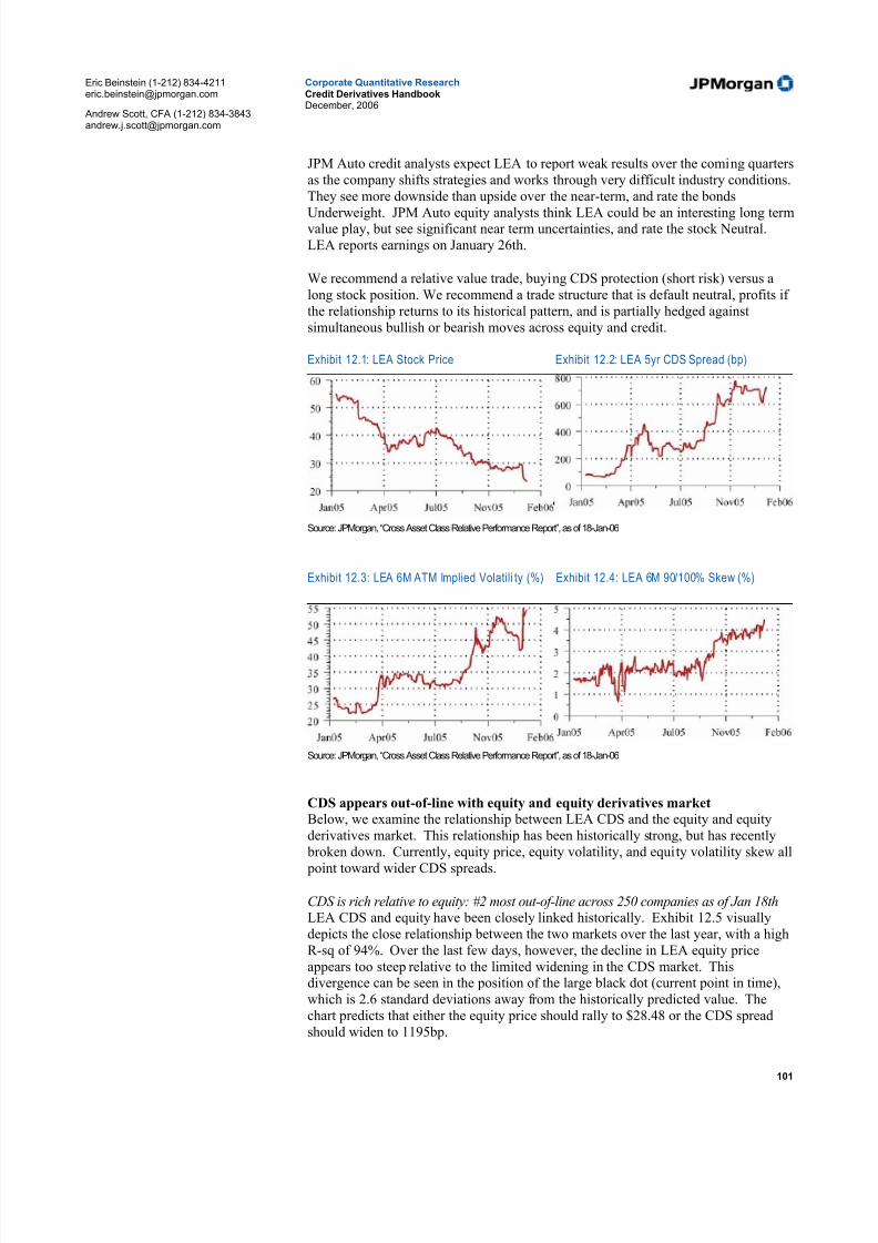
5/10/2018 JPM Credit Derivatives - slidepdf.com
http://slidepdf.com/reader/full/jpm-credit-derivatives-559e0102dc371 101/180
Eric Beinstein (1-212) [email protected]
Andrew Scott, CFA (1-212) [email protected]
Corporate Quantitative ResearchCredit Derivatives HandbookDecember, 2006
101
JPM Auto credit analysts expect LEA to report weak results over the coming quartersas the company shifts strategies and works through very difficult industry conditions.They see more downside than upside over the near-term, and rate the bonds
Underweight. JPM Auto equity analysts think LEA could be an interesting long termvalue play, but see significant near term uncertainties, and rate the stock Neutral.LEA reports earnings on January 26th.
We recommend a relative value trade, buying CDS protection (short risk) versus along stock position. We recommend a trade structure that is default neutral, profits if the relationship returns to its historical pattern, and is partially hedged againstsimultaneous bullish or bearish moves across equity and credit.
Exhibit 12.1: LEA Stock Price Exhibit 12.2: LEA 5yr CDS Spread (bp)
Source: JPMorgan, “Cross Asset Class Relative Performance Report”, as of 18-Jan-06
Exhibit 12.3: LEA 6M ATM Implied Volatili ty (%) Exhibit 12.4: LEA 6M 90/100% Skew (%)
Source: JPMorgan, “Cross Asset Class Relative Performance Report”, as of 18-Jan-06
CDS appears out-of-line with equity and equity derivatives marketBelow, we examine the relationship between LEA CDS and the equity and equityderivatives market. This relationship has been historically strong, but has recently broken down. Currently, equity price, equity volatility, and equity volatility skew all
point toward wider CDS spreads.
CDS is rich relative to equity: #2 most out-of-line across 250 companies as of Jan 18thLEA CDS and equity have been closely linked historically. Exhibit 12.5 visuallydepicts the close relationship between the two markets over the last year, with a highR-sq of 94%. Over the last few days, however, the decline in LEA equity priceappears too steep relative to the limited widening in the CDS market. Thisdivergence can be seen in the position of the large black dot (current point in time),which is 2.6 standard deviations away from the historically predicted value. Thechart predicts that either the equity price should rally to $28.48 or the CDS spreadshould widen to 1195bp.

5/10/2018 JPM Credit Derivatives - slidepdf.com
http://slidepdf.com/reader/full/jpm-credit-derivatives-559e0102dc371 102/180
Eric Beinstein (1-212) [email protected]
Andrew Scott, CFA (1-212) [email protected]
Corporate Quantitative ResearchCredit Derivatives HandbookDecember, 2006
102
Exhibit 12.5: LEA Debt vs. Equity Relations hip, 1 yr regression
Source: JPMorgan, “Cross Asset Class Relative Performance Report”, as of 18-Jan-06
CDS is rich relative to equity volatility: #1 most out-of-line across 250 companies as
of Jan 18thLEA CDS and equity volatility have also been closely linked historically. Exhibit12.6 visually depicts the close relationship between the two markets over the lastyear, with an R-sq of 93%. Over the last few days, the increase in LEA equityvolatility appears too high relative to the limited widening in the CDS market. Thisdivergence can be seen in the position of the large black dot (current point in time),which is 2.8 standard deviations away from the historically predicted value. Thechart predicts that either the equity volatility should fall to $48.31 or the CDS spreadshould widen to 885bp.
Exhibit 12.6: LEA Debt vs. Equity Vol Relations hip, 1 yr regression Exhibit 12.7: LEA Equity vs. Equity Skew Relationshi p, 1 yr regression
Source: JPMorgan, “Cross Asset Class Relative Performance Report”, as of 18-Jan-06
Each dot on the chartrepresents one day, with thelarger dots representingmore recent points in timeand the black dotrepresenting the current day.The black line represents theregression “predicted”value, and the two grey linesrepresent two standarddeviations from that value.

5/10/2018 JPM Credit Derivatives - slidepdf.com
http://slidepdf.com/reader/full/jpm-credit-derivatives-559e0102dc371 103/180
Eric Beinstein (1-212) [email protected]
Andrew Scott, CFA (1-212) [email protected]
Corporate Quantitative ResearchCredit Derivatives HandbookDecember, 2006
103
CDS is rich relative to skew: #1 most out-of-line across 250 companies as of Jan
18thFinally, we note that CDS and the equity volatility skew have also been closelylinked. In this case, equity skew has been increasing (indicating that OTM putvolatility is being bid up by investors buying put protection, likely a bearish signal)in step with widening in the CDS market. Exhibit 12.7 depicts the close relationship between the two markets over the last year, with an R-sq of 77%. Over the last fewdays, the increase in LEA skew appears too high relative to the limited widening inthe CDS market. This divergence can be seen in the position of the large black dot(current point in time), which is 1.9 standard deviations away from the historically predicted value. The chart predicts that either skew should fall to 3.71 vols or theCDS spread should widen to 951bp.
Trade Structure DiscussionWe present our recommendation on how to structure this trade and the characteristics
of the resulting pair of positions, with each column in Exhibit 12.8 discussed in moredetail below.
Exhibit 12.8: Trade Recommendation and Sensitivities
(1) (2) (3) (4) (5) (6) (7)
Entry Regression P/L if Move 3month P/L in
Buy/ Size Level ($)/ Predic ted to Predic ted Carry Default
Sell ($'000) Spread (bp) Pric e/Spread ($'000) ($'000) ($'000)
Long Stock Buy $5109 $23.31 $28.48 $1,133 $55 -$5,000
CDS 5Yr Buy (short risk) $10,000 725bp 1195bp $1,548 -$181 $5,000
-$126 $0
Source: JPMorgan, as of 18-Jan-06
1) We recommend buying the stock and buying CDS protection (short risk).We expect stock price to rise and/or the CDS spread to widen.
2) The two legs of the trade are sized to have equivalent P/L in default (i.e. welose the same amount on the long stock position as we gain on the CDS position in the event of default). See column 7 for more detail. A $5109 position in the stock equates to 180,685 shares.
3) We show the current equity price and CDS spread. The CDS spread is the5yr Credit Default Swap spread, or what one would pay annually in basis points to enter a short risk CDS position.
4) We show the predicted equity price, assuming no change in CDS and theequity price moves up to meet the regression line in Exhibit 12.5 above. The predicted CDS level is calculated similarly, but assuming the equity price isunchanged and CDS moves right to the predicted point in the regression. Inthe P/L grid below we illustrate the combined results of the positions acrossa range of stock price and CDS levels.
5) Stock P/L = change in stock price if move to predicted * number of shares.CDS P/L = change in spread / 10,000 * duration * notional
6) The carry on the equity leg is the dividend yield and on the CDS leg it is thespread - in both cases multiplied by the size of each position and shown as aquarterly figure. This position has a negative carry.

5/10/2018 JPM Credit Derivatives - slidepdf.com
http://slidepdf.com/reader/full/jpm-credit-derivatives-559e0102dc371 104/180
Eric Beinstein (1-212) [email protected]
Andrew Scott, CFA (1-212) [email protected]
Corporate Quantitative ResearchCredit Derivatives HandbookDecember, 2006
104
7) We show the loss on each leg of the position assuming a jump to default.For the equity leg we assume $0.50 price in default and for the CDS leg weassume a recovery rate or value of bonds post a default of 50%. The 50%
recovery is in the range of likely scenarios according to our credit analyst,and is in line with current pricing on recovery rate swaps (see “profitingfrom views on recovery rates” article in this publication). This combined position has zero P/L in default under these assumptions. In practice, if recovery on the credit is higher than 50%, P/L will be negative. If recoveryon the credit is less than 50%, P/L will be positive.
Profit/Loss on PositionBelow we present a grid of profit/loss on the position as recommended above. Thefigures in the grid are dollars, in thousands, assuming the sizes of the positiondiscussed above. As there are different amounts at risk in the equity and CDS legs of the trade, showing P/L in dollars rather than as a percentage of risk is preferable. Theresult with the square is the P/L with unchanged stock price and CDS spread. It is
negative reflecting the negative carry in the trade. Note that the trade makes the most money if equity prices increase and CDS spreadswiden. Although this scenario is possible, it is not the most likely. We believescenarios where CDS spreads widen and equity prices are unchanged (move right onthe grid) or equity price rallies and CDS is unchanged (move up on the grid) aremore likely. Note that P/L volatility is relatively low for bullish or bearish movesacross both equity and credit. For example, the P/L for CDS widening to 885bpcombined with a $2.00 drop in the stock price is $102k, similar to the $126k in theunchanged scenario. In this way, the position isolates changes in the relationship between equity and CDS, while partially hedging against overall market direction.
Exhibit 12.9: Payout Diagram in 3 months: P/L ($thousand) on the combined positions
485 565 645 725 805 885 965 1045 112
32.55 1,065 1,353 1,622 1,874 2,110 2,331 2,539 2,734 2,916
30.31 580 868 1,137 1,389 1,625 1,846 2,054 2,248 2,431
29.31 365 652 921 1,173 1,409 1,631 1,838 2,033 2,216
27.31 (68) 219 488 740 976 1,197 1,405 1,600 1,782
25.31 (5 02 ) (2 14 ) 55 307 543 764 972 1,166 1,349
23.31 (935) (648 ) (37 8) (126) 110 331 539 733 916
21.31 (1,368) (1,081 ) (81 2) (5 60) (32 3) (1 02) 105 300 483
19.31 (1,801) (1,514 ) (1,24 5) (9 93) (75 7) (5 35) (328) (133) 50
17.31 (2 ,2 34 ) (1 ,9 47 ) (1 ,6 78 ) ( 1,4 26 ) (1 ,19 0) (9 69 ) ( 76 1) ( 56 6) (3 84
15.31 ( 2, 66 8) ( 2 ,3 80 ) ( 2, 11 1) ( 1 ,8 59 ) ( 1, 62 3) ( 1 ,4 02 ) ( 1, 19 4) ( 99 9) ( 81 7
13.31 (3,101) (2,813) (2,544) (2,292) (2,056) (1,835) (1,627) (1,433) (1,250
CDS Spread (bp)
E q u i t y
P r i c e
( $ )
Source: JPMorgan

5/10/2018 JPM Credit Derivatives - slidepdf.com
http://slidepdf.com/reader/full/jpm-credit-derivatives-559e0102dc371 105/180
Eric Beinstein (1-212) [email protected]
Andrew Scott, CFA (1-212) [email protected]
Corporate Quantitative ResearchCredit Derivatives HandbookDecember, 2006
105
A successful debt/equity tradeOn Jan 25, 2006, the stock had risen 8% while the CDS spread widened 30bp. Wegained profits on both legs of the trade and therefore closed the position.
Exhibit 12.10: Closed Trade MTM P/L
(1) (2) (3) (4) (5)
Entry Closing P/L
Buy / Size Level($)/ Price/ Closing
Sell ($'000) Spread (bp) Spread (bp) Pric e/ Spread
Long Stock Buy 5,109 $23.31 $25.12 $395
CDS 5Yr Buy (short risk) 10,000 725bp 755bp $100
$495
Source: JPMorgan, as of 25-Jan-06
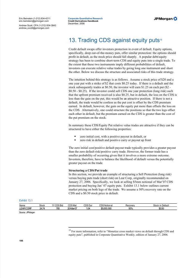
5/10/2018 JPM Credit Derivatives - slidepdf.com
http://slidepdf.com/reader/full/jpm-credit-derivatives-559e0102dc371 106/180
Eric Beinstein (1-212) [email protected]
Andrew Scott, CFA (1-212) [email protected]
Corporate Quantitative ResearchCredit Derivatives HandbookDecember, 2006
106
13. Trading CDS against equity puts19
Credit default swaps offer investors protection in event of default. Equity options,specifically, deep out-of-the-money puts, offer similar protection: the options should
profit in default, as the stock price should fall sharply. A popular debt/equity
strategy has been to combine short-term CDS and equity puts into a single trade. To
the extent that these two instruments imply different probabilities of default,
investors can execute relative value trades by going long one instrument and short
the other. Below we discuss the structure and associated risks of this trade strategy.
The intuition behind this strategy is as follows. Assume a stock price of $20 and a
one year put with a strike of $2 that costs $0.25 today. If there is a default and the
stock subsequently trades at $0.50, the investor will earn $1.25 on each put ($2 -
$0.50 - $0.25). If the investor could sell CDS one year protection (long risk) such
that the upfront premium received is also $0.25, but in default, the loss on the CDS is
less than the gain on the put, this would be an attractive position. If there is not a
default, the trade would be costless as the put cost is offset by the CDS premium
earned. In default, however, the gain on the equity put more than offsets the loss on
the CDS. Alternatively, one could structure the positions so that the two legs offset
each other in default, but the premium earned on the CDS is greater than the cost of
the put premium on the stock.
In summary these CDS/Equity Put relative value trades are attractive if they can be
structured to have either the following properties:
zero initial cost, with a positive payout in default, or zero risk in default and positive carry or payout up front
The zero initial cost/positive default payout trade typically provides a greater payout
than the zero default risk/positive carry trade. However, the former trade has a
smaller probability of occurring given that it involves a more extreme outcome.
Investors, therefore, have to balance the likelihood of default versus the potentially
greater payout on the trade.
Structuring a CDS/Put trade
In this section, we provide an example of structuring a Sell Protection (long risk)
versus buying puts trade (short risk) on Lear Corp, originally recommended on
January 27, 2006. Specifically, we look at selling $5mm notional of Mar’07 CDS
protection and buying Jan’ 07 equity puts. Exhibit 13.1 below outlines current
market pricing on both legs of the trade. We assume a 50% recovery rate on the
CDS and a $0.50 stock price in default.
Exhibit 13.1
Name Stock 1Y CDS Bid CDS Mat CDS Dur CDS Notion al Recovery Stock in DefaultLEAR CORP 24.74 785 20-Mar-07 1.04 $5,000,000 50% $0.50
Source: JPMorgan
19For more information, refer to “Monetize cross market views on default through CDS and
equity puts”, published in Corporate Quantitative Weekly, edition of January 27, 2006.

5/10/2018 JPM Credit Derivatives - slidepdf.com
http://slidepdf.com/reader/full/jpm-credit-derivatives-559e0102dc371 107/180
Eric Beinstein (1-212) [email protected]
Andrew Scott, CFA (1-212) [email protected]
Corporate Quantitative ResearchCredit Derivatives HandbookDecember, 2006
107
In Exhibit 13.2, we examine the P/L on this trade using different put strikes. In each
scenario, we calculate the number of puts needed, such that, in default the positive
P/L from the puts purchased is equivalent to the negative P/L from the long risk CDS
position. For example, at a $10 put strike, 2,632 put contracts are needed to generate$2.5mm in default assuming the stock falls to $0.50, which is the amount lost on the
long risk CDS position.
Continuing this example, at a cost of $0.95 per contract, the cost of buying 2,632
puts is $250k, which is $158k less than the premium received from the long risk
CDS position. This $158k is the positive carry on the position. Since this carry is
larger than the carry on higher strike puts, the $10 strike put appears most attractive.
Exhibit 13.2
Default-Neutral Structur es: Sell Mar' 07 CDS Protection/Buy Jan' 07 Equity PutsStrike Put Premium CDS PV1 Loss in Default on CDS2 Gain in Default on Puts3 Put Contracts4 Put Hedge Cost5 Carry6 $10.00 $0.95 $408,200 $2,500,000 $2,500,000 2,632 $250,000 $158,200
$12.50 $1.35 $408,200 $2,500,000 $2,500,000 2,083 $281,250 $126,950$15.00 $1.90 $408,200 $2,500,000 $2,500,000 1,724 $327,586 $80,614$17.50 $2.50 $408,200 $2,500,000 $2,500,000 1,471 $367,647 $40,553$20.00 $3.30 $408,200 $2,500,000 $2,500,000 1,282 $423,077 -$14,877$25.00 $5.30 $408,200 $2,500,000 $2,500,000 1,020 $540,816 -$132,616$30.00 $8.10 $408,200 $2,500,000 $2,500,000 847 $686,441 -$278,241
1. CDS PV is the present value of payments received for selling protection. For names trading in all running spread form (names trading at typically less than 1000bp), the calculation is
Spread/10000 * Duration. $408,200 = 785/10000 * 1.04 * $5MM
2. Loss in Default is calculated as CDS Notional * (1 - Recovery). We assume recovery is 50%
3. Gain in Default is set to be the same as the loss on CDS so as to be default-neutral
4. Number of put contracts is set so as to achieve the required gain in default (column to the left). Number of contracts = Gain in Default on Puts / (100 * (K - Stock price in default))
5. Put hedge cost = Number of Put contracts * 100 * Put Premium
6. Carry = CDS PV - Put Hedge Cost
Source: Bloomberg, JPMorgan
Note, however, that the assumption of a 50% recovery affects the amount of puts we
need to buy in order to offset the loss on the CDS in default. If the actual recoveryrate was lower, then the CDS position would lose more money in default, and wewould need to have bought more puts to have a default neutral trade. In other words,the trade in Exhibit 13.2 is left exposed to the actual recovery rate. This exposurecan be significant. Exhibit 13.3 outlines the impact of recovery on the defaultexposure. Whereas our trade (at any strike) is default neutral, a realized recoverylower than 50% creates a negative default P/L and a realized recovery above 50%creates a positive default P/L.
Exhibit 13.3
Trade P/L for given Recovery20% 40% 50% 60% 80%
-$1,500,000 -$500,000 $0 $500,000 $1,500,000
Note: P/L is calculated as the difference between CDS payout in event of default and gain on puts.
Source: JPMorgan
Recovery rate swaps can be used to hedge recovery exposure. Typically, only
distressed companies are traded in the recovery rate market. Intuitively, this is
because investors are more interested in taking views on recovery for names that may
actually default. Currently, several auto and auto-parts companies trade in the
recovery rate swap market. We list them and recovery rates below:

5/10/2018 JPM Credit Derivatives - slidepdf.com
http://slidepdf.com/reader/full/jpm-credit-derivatives-559e0102dc371 108/180
Eric Beinstein (1-212) [email protected]
Andrew Scott, CFA (1-212) [email protected]
Corporate Quantitative ResearchCredit Derivatives HandbookDecember, 2006
108
Company Recovery Rate SwapGM 38 / 40DANA 49 / 53LEAR 47 / 57
AXL 53 / 63Note: Indicative levels as of January 25, 2005
Source: JPMorgan
A level of 53/63, for instance, means that investors can sell protection at a fixed
recovery of 53% (i.e. they will pay 47 in event of default) and buy protection on a
vanilla CDS. Conversely, investors can buy protection at a fixed recovery of 63%
(i.e. they receive 37% in event of default) and sell protection on a vanilla CDS.
(Please see Part IV for more details on recovery rate swaps).
Incorporating a fixed recovery rate swap leg to our trade produces the following
trade structure (Exhibit 13.4). Sell Mar’ 07 Fixed Recovery CDS Protection @ 47%
fixed recovery (current LEA recovery swap Bid) versus buying Jan ’07 equity puts.
In event of default, we lose 53% of the notional on the CDS.
Note that for each strike, the trade requires more put contracts since the recovery rate
is lower (CDS loses 53% rather than 50% in default). Because of the need to buy
more puts, the carry is reduced. In all other aspects the trade is the same, and is no
longer sensitive to changes in actual realized recovery.
Exhibit 13.4
Default-Neutral Structur es: Sell Mar' 07 Fixed Recovery CDS Protection/Buy Jan '07 Equity PutsStrike Put Premium CDS PV CDS Default Exposure1 Gain in Default on Puts Put Contracts Put Hedge Cost Carry$10.00 0.95 $392,500 $2,650,000 $2,650,000 2,789 $265,000 $127,500$12.50 1.35 $392,500 $2,650,000 $2,650,000 2,208 $298,125 $94,375$15.00 1.90 $392,500 $2,650,000 $2,650,000 1,828 $347,241 $45,259$17.50 2.50 $392,500 $2,650,000 $2,650,000 1,559 $389,706 $2,794
$20.00 3.30 $392,500 $2,650,000 $2,650,000 1,359 $448,462 -$55,962$25.00 5.30 $392,500 $2,650,000 $2,650,000 1,082 $573,265 -$180,765$30.00 8.10 $392,500 $2,650,000 $2,650,000 898 $727,627 -$335,127
1. CDS Default Exposure is calculated as CDS Notional * (1 - 47%)
Source: Bloomberg, JPMorgan
Risks to the strategyThere are several risks inherent in this strategy:
• MTM volatility can be significant. CDS and puts have different risk profiles and, being different capital structure instruments, may react to company news in anunanticipated way. For example, a LBO announcement is likely to push spreadswider and the stock higher, hurting the investor in a sell CDS/buy Put trade on
both legs.
• Recovery on CDS has a large impact on the trade payoff. Trading a fixedrecovery CDS against the put hedges recovery rate risk. However, as we note below, the recovery rate market typically trades only distressed names, so the pool of potential trades is significantly smaller.
• Maturities between the CDS and equity puts may differ. CDS typically trade tothe 20th of March, June, September and December, which often creates amismatch with an exchange-traded puts. Tailoring a CDS or equity puts to a particular maturity may often be very difficult or prohibitively expensive.Another alternative may be to roll the option as maturity approaches, since thereare more short-term than long-term option maturities available to an investor.

5/10/2018 JPM Credit Derivatives - slidepdf.com
http://slidepdf.com/reader/full/jpm-credit-derivatives-559e0102dc371 109/180
Eric Beinstein (1-212) [email protected]
Andrew Scott, CFA (1-212) [email protected]
Corporate Quantitative ResearchCredit Derivatives HandbookDecember, 2006
109
• The final stock price will also affect the trade payoff
Option Buyer. Options are a decaying asset, and investors risk losing 100% of the
premium paid.
Put Sale. Investors who sell put options will own the underlying stock if the stock price falls below the strike price of the put option. Investors, therefore, will beexposed to any decline in the stock price below the strike potentially to zero, andthey will not participate in any stock appreciation if the option expires unexercised.
Analyzing Fixed Recovery CDS/Put Trades
Below, we show a similar fixed recovery CDS/Put analysis for a number of
companies that trade in the recovery rate market. We show both the zero carry as
well as zero payoff in default scenarios.
Exhibit 13.5: Three names that trade in the recovery rate market
Name Stock 1Y CDS Bid Points CDS Dur CDS Not CDS Recovery Bid Stock in Def General Motors $22.58 500bp 8.5 0.90 $5,000,000 38 $0.50American Axle $18.37 555bp 0 1.06 $5,000,000 53 $0.50Dana Corp 4.44 500bp 16 0.80 $5,000,000 49 $0.50
Source: JPMorgan, Bloomberg
Exhibit 13.6: Sell Fixed Recovery CDS/Buy Equit y Puts Trades
Trade: Zero Carry, Positive Payoff in Default1 Trade: Default-Neutral,
Positive Carry2
NameStrikePrice
PutPremium CDS PV
PutContracts
Loss in Defaulton CDS
Gain in Defaulton Puts Total # Contracts Cost Payoff
General Motors $2.50 $0.25 $650,000 26000 -$3,100,000 $5,200,000 $2,100,000 15,500 $387,500 $262,500American Axle $12.50 $1.25 $294,150 2353 -$2,350,000 $2,823,840 $473,840 1,958 $244,792 $49,358Dana Corp $2.50 $0.70 $1,000,000 14286 -$2,575,000 $2,857,143 $282,143 12,875 $901,250 $98,750
Source: JPMorgan
Note: Payoff in default assumes stock trades at $0.50
Implications for put skew in the equity market
The potential to trade CDS against equity helps to anchor out-of-the-money put
pricing in the equity derivatives market. Specifically, the CDS/Equity put
relationship we describe above provides a lower bound to the put implied volatility
skew. If the skew is insufficiently steep (i.e. deep out-of-the-money puts are cheap
relative to CDS), investors can sell protection and buy puts. The upper bound for the
skew is anchored by the ability to execute put spreads (buy one put, sell farther out-
of-the-money puts). If the skew is too steep, investors can buy 1 put with strike K
and sell two puts with strike K/2. The final payoff of this trade cannot be negative or an arbitrage is created.
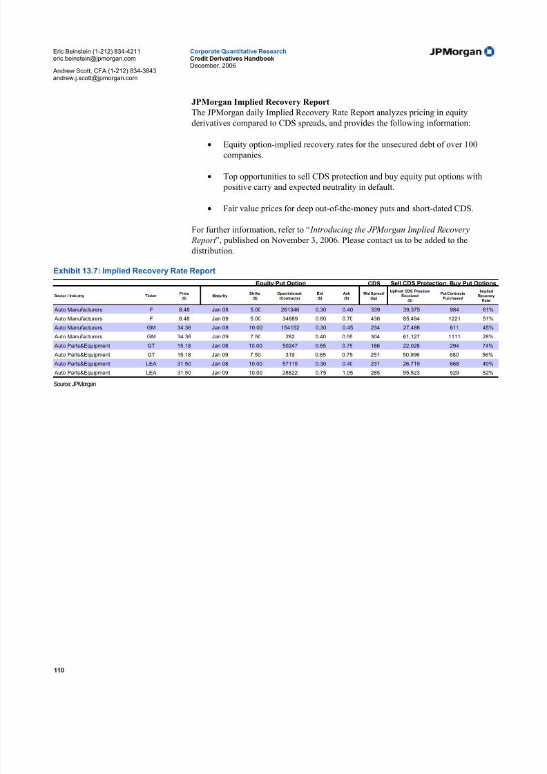
5/10/2018 JPM Credit Derivatives - slidepdf.com
http://slidepdf.com/reader/full/jpm-credit-derivatives-559e0102dc371 110/180
Eric Beinstein (1-212) [email protected]
Andrew Scott, CFA (1-212) [email protected]
Corporate Quantitative ResearchCredit Derivatives HandbookDecember, 2006
110
JPMorgan Implied Recovery Report
The JPMorgan daily Implied Recovery Rate Report analyzes pricing in equity
derivatives compared to CDS spreads, and provides the following information:
• Equity option-implied recovery rates for the unsecured debt of over 100
companies.
• Top opportunities to sell CDS protection and buy equity put options with
positive carry and expected neutrality in default.
• Fair value prices for deep out-of-the-money puts and short-dated CDS.
For further information, refer to “ Introducing the JPMorgan Implied Recovery
Report ”, published on November 3, 2006. Please contact us to be added to the
distribution.
Exhibit 13.7: Implied Recovery Rate Report CDS
Sector / Industry TickerPrice
($)Maturity
Strike1
($)
Open Interest
(Contracts)
Bid
($)
Ask
($)
Mid Spread2
(bp)
Upfront CDS PremiumReceived3
($)
Put Contracts
Purchased4
ImpliedRecovery
Rate5
Auto Manufacturers F 8.48 Jan 08 5.00 261346 0.30 0.40 339 39,375 984 61%
Auto Manufacturers F 8.48 Jan 09 5.00 34889 0.60 0.70 436 85,494 1221 51%
Auto Manufacturers GM 34.36 Jan 08 10.00 154152 0.30 0.45 234 27,486 611 45%
Auto Manufacturers GM 34.36 Jan 09 7.50 282 0.40 0.55 304 61,127 1111 28%
Auto Parts&Equipment GT 15.18 Jan 08 10.00 50247 0.65 0.75 186 22,028 294 74%
Auto Parts&Equipment GT 15.18 Jan 09 7.50 319 0.65 0.75 251 50,996 680 56%
Auto Parts&Equipment LEA 31.50 Jan 08 10.00 57115 0.30 0.40 231 26,719 668 40%
Auto Parts&Equipment LEA 31.50 Jan 09 10.00 28822 0.75 1.05 285 55,523 529 52%
Equity Put Option Sell CDS Protection, Buy Put Options
Source: JPMorgan

5/10/2018 JPM Credit Derivatives - slidepdf.com
http://slidepdf.com/reader/full/jpm-credit-derivatives-559e0102dc371 111/180
Eric Beinstein (1-212) [email protected]
Andrew Scott, CFA (1-212) [email protected]
Corporate Quantitative ResearchCredit Derivatives HandbookDecember, 2006
111
Part III: Index products
14. Credit default swap index products................................................................112Introduction .......................................................................................................112Mechanics of the CDX and iTraxx indices........................................................112Basis to theoretical ............................................................................................113Comparing on-the-run and off-the-run basis .....................................................114Credit events......................................................................................................115CDX and iTraxx indices....................................................................................116History of US CDS Indices ...............................................................................120
15. CDX and iTraxx options..................................................................................121Product description............................................................................................121Basic option strategy payoff diagrams ..............................................................122
Using options to express a spread view.............................................................122Using options to express a volatility view.........................................................122Combining spread and volatility views .............................................................123Option trading strategies....................................................................................124The practical side to trading options..................................................................125
16. Trading credit volatility ..................................................................................130Defining volatility .............................................................................................130Delta-hedging ....................................................................................................131The returns from delta-hedging in credit...........................................................132Historical analysis .............................................................................................133Option glossary..................................................................................................134
17. Tranche products.............................................................................................136What is a tranche? .............................................................................................136Why are synthetic tranches traded? ...................................................................139The mechanics of trading tranche protection.....................................................141The role of correlation.......................................................................................142Pricing tranches .................................................................................................143Other products ...................................................................................................146
5/10/2018 JPM Credit Derivatives - slidepdf.com
http://slidepdf.com/reader/full/jpm-credit-derivatives-559e0102dc371 112/180
Eric Beinstein (1-212) [email protected]
Andrew Scott, CFA (1-212) [email protected]
Corporate Quantitative ResearchCredit Derivatives HandbookDecember, 2006
112
14. Credit default swap index products
IntroductionCredit default swap indices are tradable products that allow investors to establishlong or short credit risk positions in specific credit markets or market segments.JPMorgan has worked with other dealers to create a global family of standardizedCDS indices. The results of this effort are the Dow Jones CDX indices for NorthAmerica and the Emerging Markets, and the iTraxx indices for Europe, Japan, andAsia (two collective ventures within the global credit derivatives dealer community).
Like the S&P 500 and other market benchmarks, the credit default swap indicesreflect the performance of a basket of assets, namely, a basket of single-name creditdefault swaps (credit default swaps on individual credits). Unlike a perpetual index,such as the S&P 500, CDS indices have a fixed composition and fixed maturities. Anew series of indices is established approximately every six months with a new
underlying portfolio and maturity date, to reflect changes in the credit market and tohelp investors maintain a relatively constant duration if they wish. Equal weight isgiven to each underlying credit in the CDX and iTraxx portfolios. If there is a creditevent in an underlying CDS, the credit is effectively removed from the indices inwhich it is included.
When a new index is launched, dubbed the “on-the-run index,” the existing indicescontinue to trade (as “off-the-run”), until maturity. Investors have the option to closetheir positions in off-the-run series and enter into new positions in the on-the-runindices, but are not obligated to do so. The on-the-run indices tend to be more liquidthan the off-the-run indices.
Mechanics of the CDX and iTraxx indices
Each CDX index is a separate, standard credit default swap contract with a fixed portfolio of credits and a fixed annual coupon. Investors will pay or receive aquarterly payment of this fixed coupon on a desired notional. As with standard creditdefault swap contracts, payments are made on the 20th of March, June, September,and December. Accrued interest is calculated on an Actual/360 basis.
While CDX and iTraxx products pay or receive a fixed coupon, they also trade in themarket. The traded level of the CDX or iTraxx is determined by supply and demand.To offset the difference between the fixed coupon and the market spread, investorsmust either pay or receive an upfront amount when a contract is created. If themarket spread of the index is tighter than the fixed coupon, for example, an investor selling protection (long risk) will be required to pay an upfront amount, as they will be receiving a greater fixed spread (coupon) than the level at which they trade. The
opposite is true if the spread on the index is wider than the fixed coupon; a buyer of protection (short risk) must pay an upfront fee, as the protection buyer is paying afixed coupon that is lower than the spread determined by the market. The upfront feeis the risky present value of the spread difference, or (spread difference) x (duration)x (notional). It can be calculated using the CDSW page on Bloomberg. To accessSeries 6 information, for example, enter: CDX6 CDS Corp [go], select the index,then type CDSW [go]. Note that HY CDX indices are quoted in price terms, thus theupfront payment is the price difference from par.

5/10/2018 JPM Credit Derivatives - slidepdf.com
http://slidepdf.com/reader/full/jpm-credit-derivatives-559e0102dc371 113/180
Eric Beinstein (1-212) [email protected]
Andrew Scott, CFA (1-212) [email protected]
Corporate Quantitative ResearchCredit Derivatives HandbookDecember, 2006
113
Exhibit 14.1: CDX CDSW model on Bloom berg
Source: Bloomberg
In addition to the market value upfront payment, investors must either pay or receivean accrued fee when entering into a new contract. An investor who has a long risk position on a coupon payment date will receive the full quarterly coupon payment,regardless of when she entered into the contract. If the contract was created in themiddle of a payment period, for example, in order to offset the “extra” amount of coupon she will receive, the seller of protection (long risk) must pay an accrued fee
upfront. This is similar to settling accrued interest on a bond
As mentioned in the Introduction, investors do not need to hold CDX or iTraxxcontracts until maturity but can close-out, or unwind positions at any time. Investorscan use the CDSW page on Bloomberg to calculate the value of unwinding anexisting CDX or iTraxx contract, just as they calculate the value of the upfront payment when entering the contract. As the HY CDX is quoted in price terms, thevalue of the unwind is the difference from par.
Basis to theoretical
The index spread is not directly based on the value of the underlying credit defaultswaps, but is set by the supply and demand of the market. This is analogous to the pricing of a closed-end mutual fund, where the traded price is based on the buying
and selling of the index, not fixed to the net asset value of the underlying securitiesdirectly.
Thus, the index spread is different from both the average spread of the underlyingcredit default swaps, and the theoretical value of the index. The theoretical value isthe duration weighted average of the underlying CDS. We compute the theoreticalvalue of the index using the following calculations:
• Observe the current market levels of the single-name CDS that have the samematurity date of the index. If the on-the-run single-name CDS has a differentmaturity date than the index, we interpolate between two points on the CDScurve.

5/10/2018 JPM Credit Derivatives - slidepdf.com
http://slidepdf.com/reader/full/jpm-credit-derivatives-559e0102dc371 114/180
Eric Beinstein (1-212) [email protected]
Andrew Scott, CFA (1-212) [email protected]
Corporate Quantitative ResearchCredit Derivatives HandbookDecember, 2006
114
• Convert the single-name CDS spreads into prices. We value each spread relativeto the fixed coupon of the index. This is analogous to entering the fixed indexcoupon as the “deal spread,” and the CDS spread as the “current spread” on the
CDSW calculator on Bloomberg. For example, if the index has a coupon of 50bp and the market spread of an underlying CDS was 75bp, we approximatethe price as par – (spread difference) x (duration). If we assume duration is 4,the result is 1 – (0.0075 - 0.0050) x 4 = $0.99.
• Once the prices for the underlying credits are calculated, we take a simpleaverage. This is the theoretical value of the index in price terms. We convertthis price into a spread using the same methodology used in the CDSWcalculator.
• The market-quoted index spread less the theoretical spread is the basis totheoretical.
If the quoted spread of the index is wider than this theoretical value, we say basis to
theoretical is positive. If the opposite is true, basis to theoretical is negative. Theterminology is different for the US High Yield CDX indices as they trade on pricerather than spread terms. When the HY CDX indices trade at a higher price than thetheoretical price implied by the underlying credits, the index is considered to betrading with a positive basis to theoretical value. For individual credits, investorsattempt to arbitrage basis by buying the cheap security and selling the expensivesecurity. This is also possible to do with the indices; however, the transaction costsinvolved with trading a basket of single-name CDS against the index need to beconsidered.
In a rapidly changing market, the index tends to move more quickly than theunderlying credits. This is because, in buying and selling the index, investors canexpress positive and negative views about the broader credit market in a single trade.
This creates greater liquidity in the indices compared with the individual credits. Asa result, the basis to theoretical for the indices tends to increase in magnitude involatile markets. In addition, CDX and iTraxx products are increasingly used tohedge and manage structured credit products. This may cause their spreads to bemore or less volatile or to diverge from cash bond indices.
Single-name North American high-grade credits typically include ModifiedRestructuring as a credit event (MR spread curve), while single-name NorthAmerican high-yield credits typically do not (NR spread curve). European creditsgenerally use Modified Modified Restructuring (MMR), which is similar to ModifiedRestructuring, except that it allows a slightly larger range of deliverable obligationsin the case of a restructuring event. However, across all indices, theoretical valuesare calculated using NR spread curves.
Comparing on-the-run and off-the-run basis
Investors commonly use the CDX indices to gain broad market exposure and to takeshort risk positions to hedge a portfolio of bonds. Because of the latter, on-the-runCDX indices often trade at a wider spread relative to their theoretical value, or at adiscount in dollar terms. For, if an investor wishes to enter into a short risk position,they usually do so in the on-the-run CDX, as opposed to the off-the-run CDX. As aresult, in spread terms, on-the-run indices usually have a more positive basis totheoretical than off-the-run indices. Further supporting this trend is the tendency of long-risk CDX investors to hold off-the-run indices longer than short-risk investors.Long-risk investors enjoy the roll down the curve, while short-risk investors usually prefer not to “overpay” for a shorter maturity index. For example, assume an investor

5/10/2018 JPM Credit Derivatives - slidepdf.com
http://slidepdf.com/reader/full/jpm-credit-derivatives-559e0102dc371 115/180
Eric Beinstein (1-212) [email protected]
Andrew Scott, CFA (1-212) [email protected]
Corporate Quantitative ResearchCredit Derivatives HandbookDecember, 2006
115
receives 100bp for taking a long-risk position in a 5-year CDX index. A year later,the same investor will still receive 100bp for a product that will now mature in onlyfour years. In an upward sloping and constant CDS curve environment, this spread
will be higher than the spread of a 4-year CDX index. An investor with a long risk position is more likely to hold an off-the-run index
Exhibit 14.2: CDX IG basis to th eoretical tends to be mor e positiv e(CDX has wider spread than und erlying) in th e on-the-run index
(bp)
Exhibit 14.3: CDX HY basis to th eoretical tends t o be more negative(CDX has a lower dollar price than underlying) in the on-the-run index.
($)
-3
-2
-1
0
1
2
3
4
5
6
Sep-05 Dec-05 Mar-06 Jun-06 Sep-06
IG5 IG6 IG7
-2.00
-1.50
-1.00
-0.50
0.00
0.50
1.00
1.50
Sep-05 Dec-05 Mar-06 Jun-06 Sep-06
HY5 HY6 HY7
Source: JPMorgan
Credit eventsThe credit default swaps in the index are equally weighted in terms of default protection; if there is a credit event in one credit, the notional value of an investor’sCDS contract will fall by 1/100, if there are 100 credits in the index. After a creditevent, in this example, the index will be comprised of 99 credits.
Consider an investor who buys $100 of protection (short risk) on an index with acoupon of 50bp. Assume a credit event occurs in one credit whose bonds fall to$0.40 per $1 face. If the position is physically settled, she will deliver one bond, purchased for $0.40 in the marketplace, with a $1 face (notional * 1/100), to theseller of protection (long risk) and receive $1 in cash. She will continue paying 50bpannually, but on the new notional value of $99.
The market spread of an index may change if there is a credit event in an underlyingcredit. Continuing our example, assume that, before the credit event, 99 of thecredits underlying the index have a spread of 50 and one credit has a spread of 1,000.Also assume that the index is trading at its theoretical value. The market spread of the index will be approximately 60bp. If the credit with a spread of 1,000 defaults,the credit is removed from the index, and the market spread of the index will now be50bp, the average of the remaining 99 credits (Exhibit 14.4). An investor who islong protection (short risk) will therefore lose money when the index spread rallies, but receive money on the credit event ($0.60 in our example). If the credit event waswidely anticipated, these two factors will likely offset one another with no significantnet impact on her profit and loss statement.
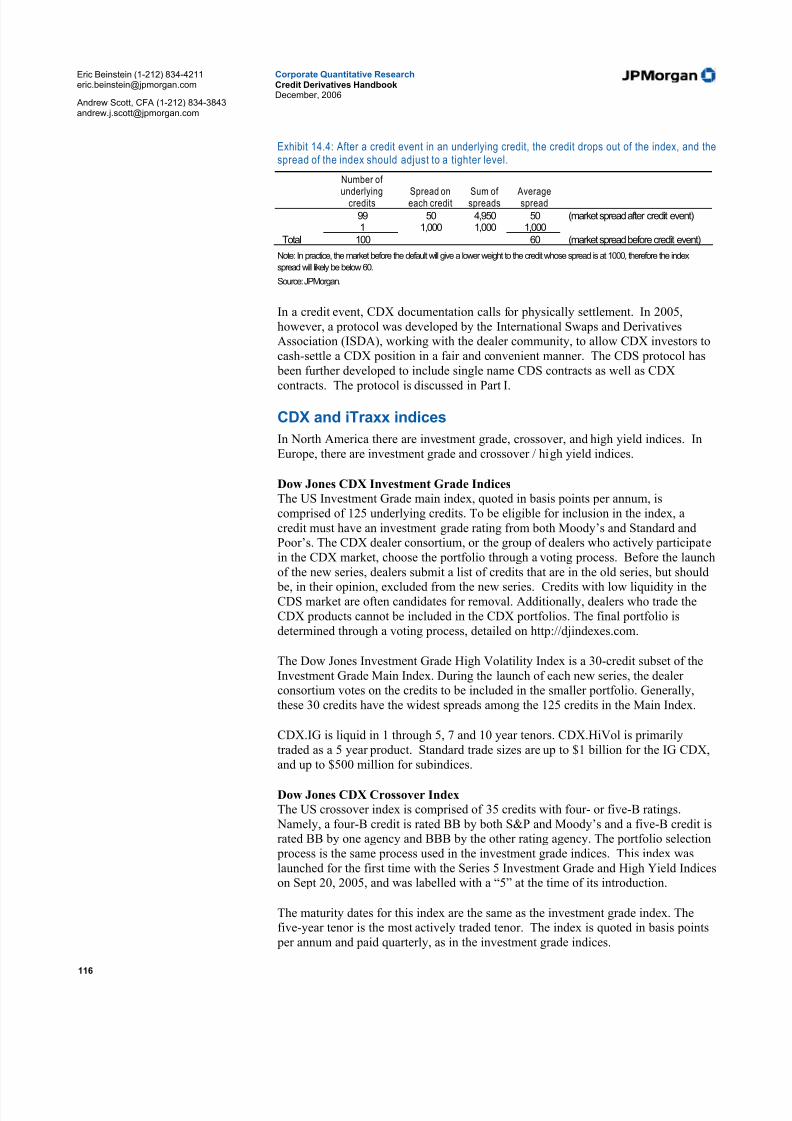
5/10/2018 JPM Credit Derivatives - slidepdf.com
http://slidepdf.com/reader/full/jpm-credit-derivatives-559e0102dc371 116/180
Eric Beinstein (1-212) [email protected]
Andrew Scott, CFA (1-212) [email protected]
Corporate Quantitative ResearchCredit Derivatives HandbookDecember, 2006
116
Exhibit 14.4: After a credit event in an underlying credit, the credit drops out of the index, and thespread of the index should adjust to a tight er level.
Number of
underlying Spread on Sum of Averagecredits each credit spreads spread99 50 4,950 50 (market spread after credit event)1 1,000 1,000 1,000
Total 100 60 (market spread before credit event)
Note: In practice, the market before the default will give a lower weight to the credit whose spread is at 1000, therefore the index
spread will likely be below 60.
Source: JPMorgan.
In a credit event, CDX documentation calls for physically settlement. In 2005,however, a protocol was developed by the International Swaps and DerivativesAssociation (ISDA), working with the dealer community, to allow CDX investors tocash-settle a CDX position in a fair and convenient manner. The CDS protocol has been further developed to include single name CDS contracts as well as CDX
contracts. The protocol is discussed in Part I.
CDX and iTraxx indices
In North America there are investment grade, crossover, and high yield indices. InEurope, there are investment grade and crossover / high yield indices.
Dow Jones CDX Investment Grade IndicesThe US Investment Grade main index, quoted in basis points per annum, iscomprised of 125 underlying credits. To be eligible for inclusion in the index, acredit must have an investment grade rating from both Moody’s and Standard andPoor’s. The CDX dealer consortium, or the group of dealers who actively participatein the CDX market, choose the portfolio through a voting process. Before the launchof the new series, dealers submit a list of credits that are in the old series, but should
be, in their opinion, excluded from the new series. Credits with low liquidity in theCDS market are often candidates for removal. Additionally, dealers who trade theCDX products cannot be included in the CDX portfolios. The final portfolio isdetermined through a voting process, detailed on http://djindexes.com.
The Dow Jones Investment Grade High Volatility Index is a 30-credit subset of theInvestment Grade Main Index. During the launch of each new series, the dealer consortium votes on the credits to be included in the smaller portfolio. Generally,these 30 credits have the widest spreads among the 125 credits in the Main Index.
CDX.IG is liquid in 1 through 5, 7 and 10 year tenors. CDX.HiVol is primarilytraded as a 5 year product. Standard trade sizes are up to $1 billion for the IG CDX,and up to $500 million for subindices.
Dow Jones CDX Crossover Index
The US crossover index is comprised of 35 credits with four- or five-B ratings. Namely, a four-B credit is rated BB by both S&P and Moody’s and a five-B credit israted BB by one agency and BBB by the other rating agency. The portfolio selection process is the same process used in the investment grade indices. This index waslaunched for the first time with the Series 5 Investment Grade and High Yield Indiceson Sept 20, 2005, and was labelled with a “5” at the time of its introduction.
The maturity dates for this index are the same as the investment grade index. Thefive-year tenor is the most actively traded tenor. The index is quoted in basis points per annum and paid quarterly, as in the investment grade indices.

5/10/2018 JPM Credit Derivatives - slidepdf.com
http://slidepdf.com/reader/full/jpm-credit-derivatives-559e0102dc371 117/180
Eric Beinstein (1-212) [email protected]
Andrew Scott, CFA (1-212) [email protected]
Corporate Quantitative ResearchCredit Derivatives HandbookDecember, 2006
117
Dow Jones CDX High Yield IndexThe Dow Jones CDX.NA.HY 100 is comprised of 100 underlying North Americancredits. The CDX dealer consortium chooses the portfolio through a voting process
similar to the Investment Grade indices. To be eligible for inclusion in the index, acredit must not have an investment grade rating from both Moody’s and Standardand Poor’s, but can have an investment grade rating from one of the two agencies.The most liquid credits are usually selected.
The High Yield index has three subindices, namely the DJ CDX.NA.HY BB, DJCDX.NA.HY B and DJ CDX.NA.HY High Beta indices. The underlying credits of the BB and B sub-indices are based on the Moody’s ratings at the time of the indices’launch. The High Beta index, like the investment grade High Volatility index, is a30-credit index determined by the dealer consortium. Generally, the 30 credit defaultswaps with the highest spreads at the time of portfolio selection are included.
Unlike the investment grade indices, the high yield CDX is quoted in dollar prices.
Furthermore, the 100, BB, and B indices are available in both swap (unfunded) andnote (funded) form.
Dow Jones CDX.NA.HY Notes: Each Dow Jones CDX.NA.HY Note is a separatetrust certificate with a fixed portfolio of credits and a fixed coupon. The notes have a prospectus and trade like bonds, with transfers of cash at the time of purchase. Likea bond, Dow Jones CDX.NA.HY Notes pay a fixed coupon on a semi-annual basis,with accrued interest calculated on a 30/360 day count convention. Payments aremade on the 20th of June and December. The CDX notes can be thought of as a package of the CDX swaps plus a trust that pays Libor. A detailed diagram of theCDX.NA.HY Notes structure is provided below.
When a new index is launched, the CDX dealer consortium draws bonds from thetrust. Dealers are able to draw from the trust, up to the amount specified in the prospectus, for up to 90 days after the CDX launch. After 90 days, dealers may beable to draw from the trust for up to one year if there has not been a credit event in anunderlying CDS. Thus, bonds may trade rich or cheap compared to theoretical valuedepending on the number of bonds drawn from the trust and the overall supply anddemand.
CDX HY Swaps settle physically or through auction after a default as describedabove in the CDX.IG discussion. CDX.HY Notes settle differently. If there is a creditevent, note holders do not need to take any action in order for a default to be settled.The settlement procedures for the notes are outlined in the offering memorandum. Insummary, the CDX dealers will hold the three auctions for bonds of the defaultedcredit. The CDX dealers deliver bonds to the auction agent over the course of thethree auctions. The auction agent then sells the bonds to the marketplace through an
auction process. The weighted average price paid by the marketplace during the threeauctions will be the recovery price. Note holders in affected indices then receive a payment of this recovery price. The entire process takes approximately four to sixweeks.
The CDX.NA.HY Note will continue to pay the original coupon amount but on areduced notional. For the 100 index, for example, each subsequent credit event willreduce the notional of a position by 1/100 of the original notional. The process is thesame for the other Dow Jones CDX.NA.HY Notes except the ratios are different, asthe original number of credits in each index is fewer than 100.
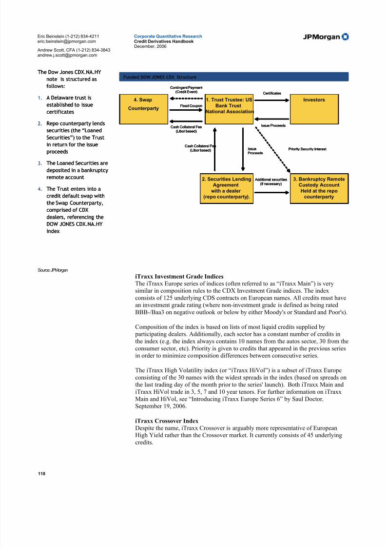
5/10/2018 JPM Credit Derivatives - slidepdf.com
http://slidepdf.com/reader/full/jpm-credit-derivatives-559e0102dc371 118/180
Eric Beinstein (1-212) [email protected]
Andrew Scott, CFA (1-212) [email protected]
Corporate Quantitative ResearchCredit Derivatives HandbookDecember, 2006
118
The Dow Jones CDX.NA.HY
note is structured as
follows:
1. A Delaware trust is
established to issue
certificates
2. Repo counterparty lends
securities (the “Loaned
Securities”) to the Trust
in return for the issue
proceeds
3. The Loaned Securities are
deposited in a bankruptcy
remote account
4. The Trust enters into acredit default swap with
the Swap Counterparty,
comprised of CDX
dealers, referencing the
DOW JONES CDX.NA.HY
index
4. Swap
Counterparty
1. Trust Trustee: USBank Trust
National Association
2. Securities LendingAgreement
with a dealer(repo counterparty).
Investors
3. Bankruptcy RemoteCustody Account
Held at the repocounterparty
Fixed Coupon
Contingent Payment(Credit Event)
Cash Collateral Fee(Libor based)
Certificates
Issue Proceeds
Additional securities(if necessary)
Cash Collateral Fee(Libor based) Issue
ProceedsPriority Security Interest
Funded DOW JONES CDX Structure
Funded DOW JONES CDX StructureThe Dow Jones CDX.NA.HY
note is structured as
follows:
1. A Delaware trust is
established to issue
certificates
2. Repo counterparty lends
securities (the “Loaned
Securities”) to the Trust
in return for the issue
proceeds
3. The Loaned Securities are
deposited in a bankruptcy
remote account
4. The Trust enters into acredit default swap with
the Swap Counterparty,
comprised of CDX
dealers, referencing the
DOW JONES CDX.NA.HY
index
4. Swap
Counterparty
1. Trust Trustee: USBank Trust
National Association
2. Securities LendingAgreement
with a dealer(repo counterparty).
Investors
3. Bankruptcy RemoteCustody Account
Held at the repocounterparty
Fixed Coupon
Contingent Payment(Credit Event)
Cash Collateral Fee(Libor based)
Certificates
Issue Proceeds
Additional securities(if necessary)
Cash Collateral Fee(Libor based) Issue
ProceedsPriority Security Interest
Funded DOW JONES CDX Structure
Funded DOW JONES CDX Structure
Source: JPMorgan
iTraxx Investment Grade Indices
The iTraxx Europe series of indices (often referred to as “iTraxx Main”) is verysimilar in composition rules to the CDX Investment Grade indices. The indexconsists of 125 underlying CDS contracts on European names. All credits must havean investment grade rating (where non-investment grade is defined as being ratedBBB-/Baa3 on negative outlook or below by either Moody's or Standard and Poor's).
Composition of the index is based on lists of most liquid credits supplied by participating dealers. Additionally, each sector has a constant number of credits inthe index (e.g. the index always contains 10 names from the autos sector, 30 from theconsumer sector, etc). Priority is given to credits that appeared in the previous seriesin order to minimize composition differences between consecutive series.
The iTraxx High Volatility index (or “iTraxx HiVol”) is a subset of iTraxx Europe
consisting of the 30 names with the widest spreads in the index (based on spreads onthe last trading day of the month prior to the series' launch). Both iTraxx Main andiTraxx HiVol trade in 3, 5, 7 and 10 year tenors. For further information on iTraxxMain and HiVol, see “Introducing iTraxx Europe Series 6” by Saul Doctor,September 19, 2006.
iTraxx Crossover Index
Despite the name, iTraxx Crossover is arguably more representative of EuropeanHigh Yield rather than the Crossover market. It currently consists of 45 underlyingcredits.

5/10/2018 JPM Credit Derivatives - slidepdf.com
http://slidepdf.com/reader/full/jpm-credit-derivatives-559e0102dc371 119/180
Eric Beinstein (1-212) [email protected]
Andrew Scott, CFA (1-212) [email protected]
Corporate Quantitative ResearchCredit Derivatives HandbookDecember, 2006
119
In order to be eligible for the Crossover index, a name must have a non-investmentgrade rating (rated BBB-/Baa3 on negative outlook or below by either Moody's or Standard and Poor's), and the spread must be at least twice the average spread of the
names in iTraxx Main (excluding financials). Additionally, no credit with a spreadgreater than 1250bp or 35% upfront can be included in the index. Subject to theseconstraints, the index is composed of the most liquid credits, based on lists submitted by participating dealers. iTraxx Crossover trades in 5 and 10 year tenors. For further information on iTraxx Crossover, see “Introducing iTraxx Crossover Series 6” bySaul Doctor, September 19, 2006.
iTraxx AsiaThe iTraxx Asia family is comprised of three main indices, the iTraxx Japan, iTraxxAsia ex Japan and iTraxx Australia. For iTraxx Japan, there are 50 names in theindex, both high-grade and high-yield names, and liquidity as proxied by tradingvolume is the main criteria for index eligibility. It is the only Asian index to trade inthe three, five and ten year tenors. Additionally, there is a 25 credit HiVol sub-index
which is widely traded in the five year tenor.
iTraxx Asia ex Japan has a similar selection criteria and there are 50 names in theindex. While there are no restrictions on the split between investment-grade and non-investment grade names, there are rules to ensure the index is broad-based andrepresentative of the Pan-Asia sphere. Currently, the Series 6 and its sub-indices onlytrade in the 5-year tenor. In terms of liquidity, activity in the sub-indices is light.
Lastly, iTraxx Australia is the smallest index comprised of 25 underlying credits withAustralia or New Zealand risks. Unlike the other two indices, there are sectoralrestrictions to ensure its diversity. It trades only in the 5-year tenor. For moreinformation, please refer to "Introducing to iTraxx Asia ex Japan Series 6" and"Introducing to iTraxx Australia Series 6" by Danny Soh, September 19, 2006 aswell as "Introducing iTraxx Japan Series 6" by Mana Nakazora and Seiko Fujiwara.
Dow Jones CDX Emerging MarketsThe CDX Emerging Markets index is currently comprised of 14 unequally-weightedsovereign credits. The construction of the portfolio, both the credit selection andweights, is determined via a voting process by the CDX dealer consortium. Beforethe launch of the new series, dealers submit a list of credits that they feel should beincluded in the new series, as well as a list of those they feel should be excluded.CDX.EM is issued in both a 5-year and 10-year tenor. Liquidity is currentlyconcentrated in the 5-year. Like the High Yield index, CDX.EM is quoted in dollar prices; however, its coupon is paid out semi-annually, not quarterly.
The CDX.EM Diversified was launched in April 2005. It has 40 equal-weightedsovereign and corporate credit default swaps. This five year index is further divided
into standard credit tranches.

5/10/2018 JPM Credit Derivatives - slidepdf.com
http://slidepdf.com/reader/full/jpm-credit-derivatives-559e0102dc371 120/180
Eric Beinstein (1-212) [email protected]
Andrew Scott, CFA (1-212) [email protected]
Corporate Quantitative ResearchCredit Derivatives HandbookDecember, 2006
120
History of US CDS Indices
Before DJ CDX.NA.IG.2 and DJ CDX.NA.HY.3, there were competing index products among dealers. In 2004, JPMorgan and other dealers worked with the DowJones Company to create and endorse a family of standardized CDS indices in boththe Investment Grade and High Yield markets. This has increased the liquidity andinnovation in credit derivative products, in our opinion.
The table below provides a brief history of current and predecessor indices.
Investment Grade Maturity Date (5Y) No. of Credits 5Y Fixed Coupon(bp)DJ TRAC-X NA Series 2 98 100
Hi Vol 40 100CDX.NA.IG.2 Main 125 60
Hi Vol 30 115DJ CDX.NA.IG.3 Main 125 50
Hi Vol 30 105
DJ CDX.NA.IG.4 Main 125 40Hi Vol 30 90DJ CDX.NA.IG.5 Main 125 45
Hi Vol 30 85DJ CDX.NA.IG.6 Main 125 40
Hi Vol 30 75DJ CDX.NA.IG.7 Main 125 40
Hi Vol 30 75
June-11
March-09
September-09
March-10
June-10
December-10
December-11
Cross Over Maturity Date (5Y) No. of Credits 5Y Fixed Coupon(bp)DJ CDX.NA.XO.5 December-10 35 200DJ CDX.NA.XO.6 June-11 35 190DJ CDX.NA.XO.7 December-11 35 165
High Yield Maturity Date (5Y) No. of Credits 5Y Fixed Coupon(%) Swaps Coupon(bp)TRAC-X NA HY 100 99 8.00% 450
BB 43 6.40% 320B 53 9.00% 520HB 32 10.00% 750
TRAC-X NA HY.2 100 100 7.38% 350BB 38 6.05% 220B 59 8.00% 410HB 33 10.13% 615
DJ CDX .NA.HY.3 100 100 7.75% 375BB 43 6.38% 225B 44 8.00% 400HB 30 10.50% 625
DJ CDX .NA.HY.4 100 98 8.25% 360BB 42 6.75% 210B 40 8.00% 340HB 28 -- 500
DJ CDX .NA.HY.5 100 100 8.75% 395BB 43 7.25% 250B 44 8.25% 340HB 30 -- 500
DJ CDX .NA.HY.6 100 100 8.625% 345BB 38 7.375% 210B 48 8.125% 300HB 30 -- 500
DJ CDX .NA.HY.7 100 100 8.637% 325BB 38 7.125% 205B 48 8.000% 300HB 30 -- 500
June-11
June-10
December-10
June-09
March-09
December-11
December-09
Note: Coupons for HY are for fixed notes
Source: JPMorgan
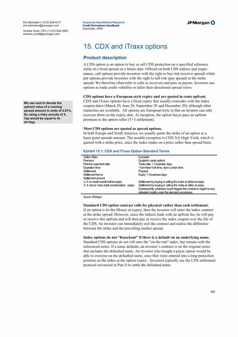
5/10/2018 JPM Credit Derivatives - slidepdf.com
http://slidepdf.com/reader/full/jpm-credit-derivatives-559e0102dc371 121/180
Eric Beinstein (1-212) [email protected]
Andrew Scott, CFA (1-212) [email protected]
Corporate Quantitative ResearchCredit Derivatives HandbookDecember, 2006
121
15. CDX and iTraxx options
Product descriptionA CDS option is an option to buy or sell CDS protection on a specified reference
entity at a fixed spread on a future date. Offered on both CDS indices and single-
names, call options provide investors with the right to buy risk (receive spread) while
put options provide investors with the right to sell risk (pay spread) at the strike
spread. We therefore often refer to calls as receivers and puts as payers. Investors use
options to trade credit volatility or tailor their directional spread views.
CDS options have a European-style expiry and are quoted in cents upfront.
CDX and iTraxx options have a fixed expiry that usually coincides with the index
coupon dates (March 20, June 20, September 20 and December 20), although other
maturities are available. All options are European-style in that an investor can only
exercise them on the expiry date. At inception, the option buyer pays an upfront
premium to the option seller (T+3 settlement).
Most CDS options are quoted as spread options.
In both Europe and North America, we usually quote the strike of an option as a
basis point spreads amount. The notable exception is CDX.NA High Yield, which is
quoted with a strike price, since the index trades on a price rather than spread basis.
Exhibit 15.1: CDX and iTraxx Option Standard Terms
Option Style: EuropeanPremium: Quoted in cents upfrontPremium payment date: Trade date + 3 business daysExpiration time: 11am New York time, 4pm London timeSettlement: Physical
Settlement terms Expiry + 3 business daysSettlement amounta. if no credit events before expiry Settlement by buying or selling the index at strike at expiryb. if one or more credit events before expiry Settlement by buying or selling the index at strike at expiry.
Subsequently, protection buyer triggers the contract in regard to anydefaulted credits under the standard procedures.
Source: JPMorgan
Standard CDS option contract calls for physical rather than cash settlement.
If an option is In-the-Money at expiry, then the investor will enter the index contract
at the strike spread. However, since the indices trade with an upfront fee, he will pay
or receive this upfront and will then pay or receive the index coupon over the life of
the CDS. An investor can immediately exit the contract and realise the difference
between the strike and the prevailing market spread.
Index options do not “Knockout” if there is a default on an underlying name.
Standard CDS options do not roll onto the "on-the-run" index, but remain with the
referenced series. If a name defaults, an investor’s contract is on the original series
that includes the defaulted name. An investor who bought a payer option would be
able to exercise on the defaulted name, once they were entered into a long protection
position on the index at the option expiry. Investors typically use the CDS settlement
protocol (reviewed in Part I) to settle the defaulted name.
We use cent to denote the
upfront value of a running
spread amount in units of 0.01%.
So using a risky annuity of 4,
1bp would be equal to 4c
(4×1bp).
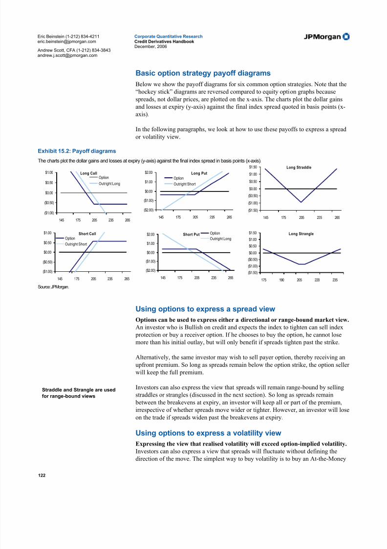
5/10/2018 JPM Credit Derivatives - slidepdf.com
http://slidepdf.com/reader/full/jpm-credit-derivatives-559e0102dc371 122/180
Eric Beinstein (1-212) [email protected]
Andrew Scott, CFA (1-212) [email protected]
Corporate Quantitative ResearchCredit Derivatives HandbookDecember, 2006
122
Basic option strategy payoff diagrams
Below we show the payoff diagrams for six common option strategies. Note that the
“hockey stick” diagrams are reversed compared to equity option graphs because
spreads, not dollar prices, are plotted on the x-axis. The charts plot the dollar gains
and losses at expiry (y-axis) against the final index spread quoted in basis points (x-
axis).
In the following paragraphs, we look at how to use these payoffs to express a spread
or volatility view.
Exhibit 15.2: Payoff diagrams
The charts plot the dollar gains and losses at expiry (y-axis) against the final index spread in basis points (x-axis).
Long Put
($2.00)
($1.00)
$0.00
$1.00
$2.00
145 175 205 235 265
Option
Outright Short
Short Put
($2.00)
($1.00)
$0.00
$1.00
$2.00
145 175 205 235 265
Option
Outright Long
Long Call
($1.00)
($0.50)
$0.00
$0.50
$1.00
145 175 205 235 265
Option
Outright Long
Short Call
($1.00)
($0.50)
$0.00
$0.50
$1.00
145 175 205 235 265
Option
Outright Short
Long Straddle
($1.50)
($1.00)
($0.50)$0.00
$0.50
$1.00
$1.50
145 175 205 235 265
Long Strangle
($1.50)
($1.00)
($0.50)
$0.00
$0.50
$1.00
$1.50
175 190 205 220 235
Source: JPMorgan.
Using options to express a spread view
Options can be used to express either a directional or range-bound market view.
An investor who is Bullish on credit and expects the index to tighten can sell index
protection or buy a receiver option. If he chooses to buy the option, he cannot lose
more than his initial outlay, but will only benefit if spreads tighten past the strike.
Alternatively, the same investor may wish to sell payer option, thereby receiving an
upfront premium. So long as spreads remain below the option strike, the option seller
will keep the full premium.
Investors can also express the view that spreads will remain range-bound by selling
straddles or strangles (discussed in the next section). So long as spreads remain
between the breakevens at expiry, an investor will keep all or part of the premium,
irrespective of whether spreads move wider or tighter. However, an investor will lose
on the trade if spreads widen past the breakevens at expiry.
Using options to express a volatility view
Expressing the view that realised volatility will exceed option-implied volatility.
Investors can also express a view that spreads will fluctuate without defining the
direction of the move. The simplest way to buy volatility is to buy an At-the-Money
Straddle and Strangle are used
for range-bound views

5/10/2018 JPM Credit Derivatives - slidepdf.com
http://slidepdf.com/reader/full/jpm-credit-derivatives-559e0102dc371 123/180
Eric Beinstein (1-212) [email protected]
Andrew Scott, CFA (1-212) [email protected]
Corporate Quantitative ResearchCredit Derivatives HandbookDecember, 2006
123
(ATM) straddle. This position is initially spread neutral in that we would make an
equal amount of money if spreads widened or tightened. We are therefore neutral to
the direction of the spreads, but will benefit from a change in spreads.
However, in order to profit, we need spreads to move more than a breakeven amount.
This breakeven is defined by the cost of the option, which in turn is defined by the
implied volatility used to price the option. If the actual spread move (realised
volatility) is greater than the breakeven (implied volatility) then the trade will be
profitable. Equation 1 shows our daily Breakeven.
Equation 1: Daily basis point volatility assuming 252 business days in a year
252
(%))(
AnnualVol ead ForwardSpr bp DailyVol
×=
where: ForwardSpread = Adjusted Forward Spread on the index in basis points20
AnnualVol = Annualised percentage volatility
Combining spread and volatility views
Investors with a view on volatility can optimize their spread view.
The Delta of an option measures how much the value of an option should change if
the underlying asset moves by one unit. Since ATM options have a delta of 50% (i.e.
a 1% change in the index P&L equates to a 0.5% change in our option P&L) we
could buy two options in order to have the same exposure as one index.
In Exhibit 15.3 we show the payoff at expiry from buying two ATM options. Here,
we take a directional view, outperforming the index if volatility is high; the options
outperform if the final spread of the index is very high or low. In Exhibit 15.4 we
have sold two ATM payer options and outperform the index if volatility is low.
Exhibit 15.3: Buying Two Payer Options Outperform ifVolatility is High
y-axis: P&L (cents); y-axis: Final Spread (bp)
-600
-400
-200
0
200
400
600
800
190 215 240 265 290 315 340 365 390 41
Option Index
Exhibit 15.4: Selling Two Payer Options Outperform ifVolatility is Low
y-axis: P&L (cents); y-axis: Final Spread (bp)
-800
-600
-400
-200
0
200
400
190 215 240 265 290 315 340 365 390 41
Option Index
Source: JPMorgan.
20CDS index options are priced using the Black formula on the CDS forward. The forward is
approximately equal to the spot plus the carry over the option term.

5/10/2018 JPM Credit Derivatives - slidepdf.com
http://slidepdf.com/reader/full/jpm-credit-derivatives-559e0102dc371 124/180
Eric Beinstein (1-212) [email protected]
Andrew Scott, CFA (1-212) [email protected]
Corporate Quantitative ResearchCredit Derivatives HandbookDecember, 2006
124
Option trading strategies
Having looked at how we can express views using payers and receivers, we look at
expressing views by combining payers and receivers.
Bull Cylinders—spreads likely to move substantially tighter, but unlikely to widen.
We form these by selling a put/payer option and buying a call/receiver option.
Between the two strikes of the trade, the cost is close to zero and the trade will
perform if spreads tighten. On the downside, if spreads move much wider, the trade
will lose money, although it outperforms an outright short protection position
(Exhibit 15.5). Variations on this strategy involve increasing the notional on one or
both legs of the trade versus the index. Bear Cylinders are formed by selling a call
and buying a put.
Bull Spreads – spreads likely to drift tighter, protection against wider spreads.
We form these by selling a low strike call and buying a high strike call (we can also
form these with puts) (Exhibit 15.6). Between the strikes of the trade, the position performs inline with the index while if spreads widen, the losses are capped above
the upper strike. The downside is that we lose, inline with the index, if spreads
widen, however, we can only lose up to the higher strike of the trade. At this point
we cap our loss. Bear spreads are also formed using different strike puts or calls.
Exhibit 15.5: Comparing a Cylinder to the Index
Payoff in Cents
-300
-200
-100
0
100
200
250 263 275 288 300 313 325 338 350 36
Option Payoff Index
Source: JPMorgan
Exhibit 15.6: Comparing a Bull Spread to the Index
Payoff in cents
-300
-200
-100
0
100
200
300
250 263 275 288 300 313 325 338 350 36
Option Payoff Index
Source: JPMorgan
Market neutral strategies
There are three common market neutral strategies available when using options:
Straddles and Strangles – spreads to remain in a range.
These are formed by selling a payer and receiver either at the same (Straddle) or at
different (Strangles) strikes. Between the breakevens, the position will make money.
The downside is that we lose if spreads widen or tighten past the breakevens (Exhibit
15.7).
Butterfly– spreads likely to remain in a range.
These are formed by selling a straddle and buying a higher strike payer option and a
lower strike receiver option. Between the breakevens, the position will make money.
Our loss is capped if we move above or below the extreme strikes, although we don't
make as much as an outright straddle.

5/10/2018 JPM Credit Derivatives - slidepdf.com
http://slidepdf.com/reader/full/jpm-credit-derivatives-559e0102dc371 125/180
Eric Beinstein (1-212) [email protected]
Andrew Scott, CFA (1-212) [email protected]
Corporate Quantitative ResearchCredit Derivatives HandbookDecember, 2006
125
Exhibit 15.7: Straddles and Strangles
-300
-200
-100
0
100
200
300
200 225 250 275 300 325 350 375 400 42
Straddle Strangle
Source: JPMorgan
Exhibit 15.8: Butterfly
Butterfly
-40
-20
0
20
40
60
80
200 225 250 275 300 325 350 375 400 42
Butterfly
Source: JPMorgan
Other option trading strategies
Calendar Spreads –trading the difference between volatility for different expiries.These are most commonly formed by trading straddles for different expiries. An
investor who believes volatility will be low in the short term, but will pick up in the
longer term may sell short-dated straddles and buy long-dated straddles. The
notionals traded can be scaled to be Vega neutral, insensitive to changes in implied
volatility, or Gamma-neutral, insensitive to changes in the index spread.
Skew Trading- trading the difference between options at different strikes
Skew measures the difference in implied volatility at different strikes. Although the
index can have only one realized volatility, supply and demand dynamics often cause
options at different strikes to trade with different levels of volatility. We tend to see
options with higher strikes trade with higher implied volatility as investors buy cheap
Out-of-the-Money payer options as portfolio protection. This causes positive skew.
Investors can trade options of different strikes to express the view that skew will
increase or decline.
The practical side to trading options
Having looked at the strategies we can use credit options for, we now look at the
practical side of trading credit options. Exhibit 15.9 shows a typical Bloomberg
screen we would see for iTraxx options (JITO <GO> on Bloomberg). Similar screens
are available for CDX and runs are send out daily from option traders.
When using index options to express a spread view, there are three aspects we
consider:
1. Cost – This is the upfront cost of an option and is the amount we pay if we buy
an option, or receive if we sell an option. This amount is quoted in cents and is an
upfront amount. Suppose an investor is concerned about spread widening and
wants to buy the option to buy protection at 26bp out to 20 March 2007. From
Exhibit 15.9 we can see that the cost of this option is 12c. On a notional trade of
$10,000,000, an investor will pay $12,000.
2. Breakeven – the trade breakeven tells us the level spreads need to be at expiry in
order to recoup the initial cost of buying the option. Continuing with our example
above, if spreads are wider than 26bp at expiry, our option will be in-the-money.
For each basis point above 26bp we will make approximately 1bp × duration. So
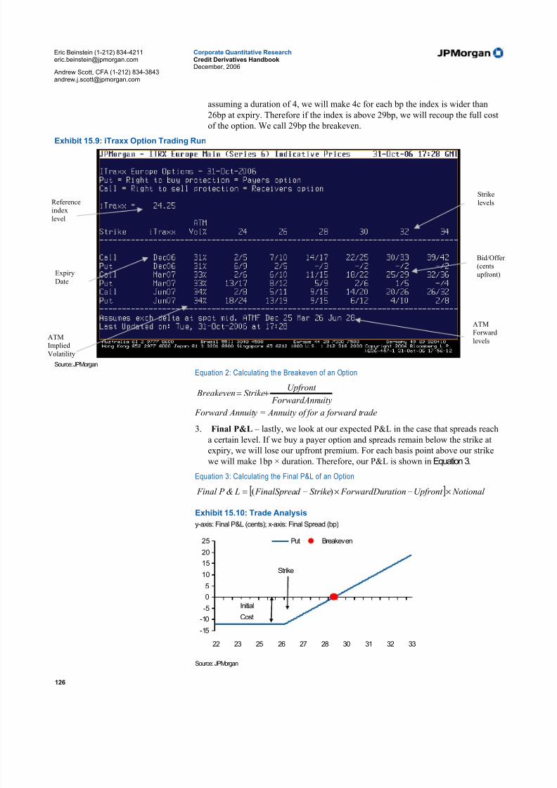
5/10/2018 JPM Credit Derivatives - slidepdf.com
http://slidepdf.com/reader/full/jpm-credit-derivatives-559e0102dc371 126/180
Eric Beinstein (1-212) [email protected]
Andrew Scott, CFA (1-212) [email protected]
Corporate Quantitative ResearchCredit Derivatives HandbookDecember, 2006
126
assuming a duration of 4, we will make 4c for each bp the index is wider than
26bp at expiry. Therefore if the index is above 29bp, we will recoup the full cost
of the option. We call 29bp the breakeven.
Exhibit 15.9: iTraxx Option Trading Run
Source: JPMorgan
Equation 2: Calculating th e Breakeven of an Option
uity ForwardAnn
Upfront Strike Breakeven +=
Forward Annuity = Annuity of for a forward trade
3. Final P&L – lastly, we look at our expected P&L in the case that spreads reach
a certain level. If we buy a payer option and spreads remain below the strike at
expiry, we will lose our upfront premium. For each basis point above our strike
we will make 1bp × duration. Therefore, our P&L is shown in Equation 3.
Equation 3: Calculating the Final P&L of an Option
[ ] Notional Upfront ation ForwardDur Striked FinalSprea L& P Final ×−×−= )(
Exhibit 15.10: Trade Analysis
y-axis: Final P&L (cents); x-axis: Final Spread (bp)
-15
-10
-5
0
5
10
15
20
25
22 23 25 26 27 28 30 31 32 33
Put Breakeven
Initial
Cost
Strike
Source: JPMorgan
Referenceindex
level
ExpiryDate
ATMImplied
Volatility
Strike
levels
Bid/Offer (cents
upfront)
ATMForward
levels

5/10/2018 JPM Credit Derivatives - slidepdf.com
http://slidepdf.com/reader/full/jpm-credit-derivatives-559e0102dc371 127/180
Eric Beinstein (1-212) [email protected]
Andrew Scott, CFA (1-212) [email protected]
Corporate Quantitative ResearchCredit Derivatives HandbookDecember, 2006
127
Delta-Exchange – the cost of trading outright
Another aspect to consider when trading options is that prices are usually quoted
with delta-exchange. This means that an investor who purchases an option with a
delta of 30% will also acquire an index position equal to 30% of the notional of thetrade. This happens because option traders need to hedge their spread exposure. A
trader who sells a $10,000,000 notional payer option with a delta of 30% and
simultaneously buys index protection on $3,000,000 notional, will initially be neutral
to spread changes in the index.
Therefore, investors who want to trade options outright and do not want this delta-
exchange will need to exit their delta position. The cost of this is just the cost of
exiting an index trade on the delta notional, Equation 4.
Equation 4: Cost of Exiting Delta
Notional AnnuityOffer Bid Cost ×××= ),(
2
1
Source: JPMorgan
Suppose we want to buy the March payer option with a strike of 26, quoted in
Exhibit 15.9, as an outright trade. The option is quoted as 8/12, so would cost us 12c
to enter. If we assume that our delta is 50% and we wish to trade outright, then we
would need to unwind our delta. If the bid/offer on the index is 0.25bp and the
annuity is 4, then the cost of this unwind is 0.5c (= 1/2×0.25bp×4). Therefore, on a
notional of $10,000,000 we would pay $12,000 for the options and $500 for the delta
unwind giving a net cost of $12,500.
The adjusted-forward – accounting for “no knockout”
We price CDS options using the forward rather than spot CDS spread. This is
because the model we use is a Black model that relies on lognormal distribution of spreads at maturity. This forward is calculated in the usual fashion (Equation 5).
Equation 5: Calculating th e Forward between time s and t
st
s st t
t s A A
AS AS F
−
−=
,
whereS t = Spreads for Maturity t
At = Risky Annuity for Maturity t
However, we adjust the forward to account for the “No Knockout” feature of
index options. If a name in the index defaults before the expiry of the option, we
will be entered into an index with a defaulted name at expiry of the option. If we had bought a payer option, we could trigger the contract and collect on the defaulted
name. Therefore, we have received protection from today, even though the forward
only offers protection from the option expiry.
We account for this additional protection by increasing the forward spread by the
cost of protection. This makes payer options more expensive and receiver options
cheaper because payer buyers receive protection on the spot and receiver buyers
forgo this protection.

5/10/2018 JPM Credit Derivatives - slidepdf.com
http://slidepdf.com/reader/full/jpm-credit-derivatives-559e0102dc371 128/180
Eric Beinstein (1-212) [email protected]
Andrew Scott, CFA (1-212) [email protected]
Corporate Quantitative ResearchCredit Derivatives HandbookDecember, 2006
128
Equation 6: Calculating the Adjustment
st
s s
A A
AS Adjustment
−=
Our adjusted-forward, which we use for pricing CDS options, is the sum of Equation
5 and Equation 6. It is roughly equal to our spot plus carry as a running spread.
Equation 7: Calculating the Adjusted Forward
uity ForwardAnn
CarrySpot
A A
AS S
A A
AS
A A
AS AS rward AdjustedFo
st
st
t
st
st
st
s st t
+≈
−+=
−+
−
−=
Exercising an option with a defaulted name in the portfolioWe present below an example on expiry mechanics for options on the Dow JonesCDX.NA.HY Swaps. The expiry mechanics for options on CDX.IG and iTraxx work similarly.
Expiry mechanics of options: The option contract is not directly affected by creditevents prior to the expiry date of the option. The option holder continues to have theright to buy or sell the “old” CDX.HY product (the product with the originalreference entities) at the agreed strike price. After exercising the option, the buyer of protection can trigger the contract under the standard procedures if he chooses.
An example below demonstrates the expiry mechanics:
• Strike = $102
• Price at expiry of “new” CDX.HY Swap (with 99 underlying credits) = $101
• Price at expiry of bonds of the credit that defaulted (recovery rate) = $0.25
Settlement process at expiry
• Investor exercises the call: he buys the “old” contract for a price of $102 (thestrike)
• The seller of the contract then triggers the defaulted name: investor pays $1.00
• Investor receives default bond worth $0.25
The net result suggests an equation that can be used to evaluate whether to exercisethe option. Exercise a long call option if:
Strike on “old” CDX.HY contract $102.00+ Defaulted credit notional value $1.00- Recovery value of defaulted credits ($0.25)
Cash cost to buy “new” DJ CDX.NA.HY through the option $102.75
Source: JPMorgan
In this example, the cash cost to buy new CDX.HY in the market is $101.00 * afactor of 0.99 = $99.99. The investor would not exercise the option, as it is $2.76 outof the money.

5/10/2018 JPM Credit Derivatives - slidepdf.com
http://slidepdf.com/reader/full/jpm-credit-derivatives-559e0102dc371 129/180
Eric Beinstein (1-212) [email protected]
Andrew Scott, CFA (1-212) [email protected]
Corporate Quantitative ResearchCredit Derivatives HandbookDecember, 2006
129
In practice, the recovery rate of the defaulted bond is determined by the CDSSettlement protocol auction process, described in Part I.
Accrued interest
An outright position pays accrued interest on a defaulted credit up to the credit eventdate. At expiry, the settlement amount for an option on the index will be adjusted toreflect the same economics.
Option pricing model
We use option pricing models either to calculate option prices from volatility levels,
or to calculate implied volatility levels from input prices.
Two such models are easily accessible to investors; JPMorgan’s Excel based model
and the CDSO Bloomberg screen. Both models use the Black pricing formula on the
forward and return very similar results. The reader is referred to Bloomberg's own
documentation on their model or to our previous note Credit Option Pricing Model
October 2004.

5/10/2018 JPM Credit Derivatives - slidepdf.com
http://slidepdf.com/reader/full/jpm-credit-derivatives-559e0102dc371 130/180
Eric Beinstein (1-212) [email protected]
Andrew Scott, CFA (1-212) [email protected]
Corporate Quantitative ResearchCredit Derivatives HandbookDecember, 2006
130
16. Trading credit volatility
Having seen the basics of option trading, we now look specifically at trading creditvolatility. The reader is referred to Trading Credit Volatility – August 2006 for more
details.
Defining volatility
Volatility in credit is a measure of the standard deviation of spreads
Volatility is defined as the annualized standard deviation of percent change in the
underlying price or spread21. For example, a volatility of 30% can be interpreted as a
68% chance (1 standard deviation) that the asset will be +/- 30% of the current level
a year from now.
We generally talk about two types of volatility:
1. Historical (also called actual, delivered or realised) volatility is the volatility of a
particular asset as measured by its past price movements
2. Implied volatility is the volatility that is forecast by the pricing of options on the
asset. This volatility is an output from the Black pricing formula for options.
Our daily basis point volatility tells us how much spreads need to change in
order to offset the cost of an option
In Credit, it is often more convenient to talk in terms of daily volatility in basis points
(basis point volatility) rather than annualised volatility in percentage terms. We can
convert annualised volatility into daily volatility in basis points using the following
formula:
Equation 8: Daily basis point volatility assuming 252 business days in a year
252)(
AnnualVol ead ForwardSpr bp DailyVol
×=
where:
ForwardSpread = Adjusted Forward Spread on the index in basis points22
AnnualVol = Annualised percentage volatility
If we think our daily spread move will exceed the breakeven then it is
worthwhile buying volatility. The breakeven, or daily volatility, therefore gives an
intuitive feel for whether options are expensive or not.
21
( )∑
−=
n
x xVol i
2
, where ⎟⎟ ⎠
⎞⎜⎜⎝
⎛ =
−1
lnt
t i
s
s x and =
t s CDS spread on day t
22CDS index options are priced using the Black formula on the CDS forward. The forward is
approximately equal to the spot plus the carry over the option term.

5/10/2018 JPM Credit Derivatives - slidepdf.com
http://slidepdf.com/reader/full/jpm-credit-derivatives-559e0102dc371 131/180
Eric Beinstein (1-212) [email protected]
Andrew Scott, CFA (1-212) [email protected]
Corporate Quantitative ResearchCredit Derivatives HandbookDecember, 2006
131
Delta-hedging
Delta-hedging involves buying an option and also an amount of the underlying index
defined by the option delta. It is designed to be neutral to the direction of spread and benefits if spreads move more than the daily breakeven.
The initial cost of an option is the cost of replication
An investor can replicate the payoff from an option by establishing and regularly
adjusting a position in the underlying index (CDX or iTraxx). The option delta tells
us the amount of the index that an investor needs to own.
As the spread on the index changes, the delta of the option will change and the
investor will need to adjust his position for the replication to work. In order to
replicate the payoff from a long call/receiver (long risk) an investor will have to sell
protection (long risk) when spreads tighten and buy protection (short risk) when
spreads widen. He will therefore buy protection at a higher spread and sell it at alower spread.
Essentially, the initial cost of an option should be equal to the cost of replicating
it. If the cost of replicating an option is more expensive than the initial cost, an
investor should buy the option and delta-hedge it. This means that he should take the
opposing position in the underlying index. An investor who buys a payer option
(short risk) should therefore sell protection (long risk) on the index in the delta
amount and adjust this hedge as the index spread moves.
Since the initial cost of an option is given by the implied volatility, and the cost of
replicating the option is given by the realised volatility, an investor who buys a delta-
hedged option will make money if realised volatility is higher than the initial implied
volatility.
Exhibit 16.1: Instantaneous P&L on Option and DeltaReplication
x-axis: CDS spread, y-axis P&L
-0.15%
-0.10%
-0.05%
0.00%
0.05%
0.10%
0.15%
0.20%
0.25%
31 32 33 35 36 37 38 39
Option P&L CDS P&L
Source: JPMorgan
Exhibit 16.2: P&L on Delta-Hedged Option over a period oftime
x-axis: CDS spread, y-axis P&L
-0.03%-0.02%
-0.01%
0.00%
0.01%
0.02%
0.03%
0.04%
0.05%
31 32 33 35 36 37 38 39
Delta Hedged Option
Source: JPMorgan
We can trade credit volatility either with a delta hedged option or with a
straddle. Rather than buying a single option and delta-hedging this over the term of
the option, a common strategy for trading volatility is to buy an ATM straddle (a call
and put at the same strike) and delta-hedge this over the option term. The straddle has
an initial delta of close to zero as the delta of the call and put net out.
The delta of an option measures
how much the theoretical value of
an option should change if the
underlying asset moves by 1 unit.
A positive delta means the
option should rise in value if the
underlying spread widens. In
credit, call deltas range between -1
and 0 while put deltas range
between 0 and 1.
Reminder:
Call = Receiver, Put = Payer

5/10/2018 JPM Credit Derivatives - slidepdf.com
http://slidepdf.com/reader/full/jpm-credit-derivatives-559e0102dc371 132/180
Eric Beinstein (1-212) [email protected]
Andrew Scott, CFA (1-212) [email protected]
Corporate Quantitative ResearchCredit Derivatives HandbookDecember, 2006
132
The returns from delta-hedging in credit
This section looks at our expected return from trading volatility, which arises due to
changes to implied volatility (Vega trading), or implied volatility differing from
realised volatility (Gamma trading).
Vega trading – changes in implied volatility: an increase in implied volatility
benefits a long option position as the options become more valuable. Vega tells us our P&L for a change in implied volatility. A delta-hedged option is
neutral to small spread changes in the underlying index. However, the P&L of such a
position will change as implied volatility changes. Higher implied volatility will
generally lead to higher option prices and an investor who is long volatility through
buying a delta-hedged option will benefit from this. For an ATM option, we can
show that:
Equation 9: Vega for an ATM Option
Implied
PriceegaV
σ ≈
where:
σ Implied = Implied Volatility of the Option
Vega trading is best performed with longer dated options as these have higher price
sensitivity to changes in implied volatility and have a lower gamma (and theta) since
the delta of the option changes less with a spread change in the underlying.
Gamma trading – differences between implied and realised volatility over the
trade horizon: realised volatility that is higher than implied should benefit a long
volatility position
Our expected P&L is dependent on the frequency of adjusting our delta-hedge
and is shown in Equation 10. In reality, a number of factors may mean that we do not
actually realise this P&L. Primarily the Black pricing formula gives us a price for an
option in a world where we can continuously buy and sell an asset in order to be
delta-neutral. In reality, continuous hedging is not feasible and we must content
ourselves with weekly, daily or inter-day hedging. The more frequently we hedge,
the more likely we are to earn our expected return.
Equation 10: Linear approximation for expected P&L from Gamma Trading
( ) Implied -ealised R Annuity Forward time L P σ σ ××××
Π
≈
2
1& .
Option traders will likely use an alternative strategy to just hedging weekly or daily.
Sometimes, they may wish to be underhedged in order to profit from changes in the
option price and not pay this away through their delta-hedge. A volatility trader
hopes not only to make his expected P&L, but to make more than this through
expedient delta-hedging.
Gamma trading is best performed with shorter dated options since our P&L from
gamma increases as we move closer to expiry (Exhibit 16.3). The higher the gamma
of our option, the more frequently we will have to adjust our delta-hedge and the
more we will be able to sell high and buy low. Higher gamma will be accompanied
by higher theta as we move towards option expiry (Exhibit 16.4).
Volatility trades seek to benefit
either from changes to implied
volatility or from realised
volatility differing from implied
volatility
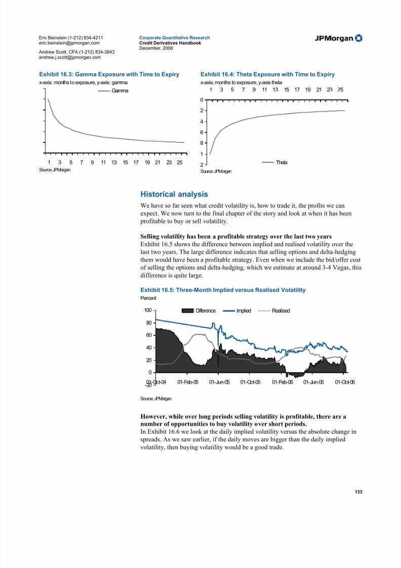
5/10/2018 JPM Credit Derivatives - slidepdf.com
http://slidepdf.com/reader/full/jpm-credit-derivatives-559e0102dc371 133/180
Eric Beinstein (1-212) [email protected]
Andrew Scott, CFA (1-212) [email protected]
Corporate Quantitative ResearchCredit Derivatives HandbookDecember, 2006
133
Exhibit 16.3: Gamma Exposure with Time to Expiry
x-axis: months to exposure, y-axis: gamma
1 3 5 7 9 11 13 15 17 19 21 23 25
Gamma
Source: JPMorgan
Exhibit 16.4: Theta Exposure with Time to Expiry
x-axis: months to exposure, y-axis theta
2
1
8
6
4
2
0
1 3 5 7 9 11 13 15 17 19 21 23 25
Theta Source: JPMorgan
Historical analysisWe have so far seen what credit volatility is, how to trade it, the profits we can
expect. We now turn to the final chapter of the story and look at when it has been
profitable to buy or sell volatility.
Selling volatility has been a profitable strategy over the last two years
Exhibit 16.5 shows the difference between implied and realised volatility over the
last two years. The large difference indicates that selling options and delta-hedging
them would have been a profitable strategy. Even when we include the bid/offer cost
of selling the options and delta-hedging, which we estimate at around 3-4 Vegas, this
difference is quite large.
Exhibit 16.5: Three-Month Implied versus Realised Volatility
Percent
-20
0
20
40
60
80
100
01-Oct-04 01-Feb-05 01-Jun-05 01-Oct-05 01-Feb-06 01-Jun-06 01-Oct-06
Difference Implied Realised
Source: JPMorgan
However, while over long periods selling volatility is profitable, there are a
number of opportunities to buy volatility over short periods.
In Exhibit 16.6 we look at the daily implied volatility versus the absolute change in
spreads. As we saw earlier, if the daily moves are bigger than the daily implied
volatility, then buying volatility would be a good trade.

5/10/2018 JPM Credit Derivatives - slidepdf.com
http://slidepdf.com/reader/full/jpm-credit-derivatives-559e0102dc371 134/180
Eric Beinstein (1-212) [email protected]
Andrew Scott, CFA (1-212) [email protected]
Corporate Quantitative ResearchCredit Derivatives HandbookDecember, 2006
134
Exhibit 16.6: Daily Implied Volatility versus Daily Move
bp
0
1
2
3
4
5
19-Oct-05 19-Dec-05 19-Feb-06 19-Apr-06 19-Jun-06 19-Aug-06
Implied Daily Change
Source: JPMorgan
Option glossary
Call – A call gives the holder the right, but not the
obligation to enter into a long risk CDS index contract at
a given spread, the strike. This is also called a receiver
option.
Put – A put gives the holder the right, but not the
obligation to enter into a short risk CDS index contract
at a given spread, the strike. This is also called a payer
option.
Straddle – A straddle is an option strategy where an
investor purchases a call and a put option with the same
strike. ATM straddles have a delta close to zero and are
therefore often used to trade volatility.
Strangle – A strangle is an options strategy similar to the
straddle, but with different strike levels for the call and
put. Strangles are frequently sold by investors who
believe the index will remain in a particular range.
Strike – The strike is the agreed spread at which CDS
index contract will be struck at maturity of the option.
Maturity – There are two maturities in a CDS option
contract. The maturity of the option and the maturity of
the underlying CDS index contract. As traded indices
have fixed maturities, the term of the index decreases as
time passes.
Adjusted Forward – The forward is the fair spread,
agreed today, at which we would enter into an index
contract at a given date in the future. We use the forward
at the option maturity to price the option. Since index
options do not knock out if a name in the underlying
index defaults, the forward spread is adjusted to account
for the additional protection this affords. If a name in the
index defaults before the maturity of the option, we will
still be entered into an index, at the options maturity, that
can be immediately triggered to collect on the defaulted
name.
At-The-Money (ATM) - An option is ATM if its strike
is equal to the forward spread on the underlying.
In-The-Money (ITM) - An option is ITM if its strike isabove the forward spread for a call and vice versa for a
put.
Out-Of-The-Money (OTM) - An option is OTM if its
strike is below the forward spread for a call and vice
versa for a put.
Realized Volatility (also known as Historic or
Delivered volatility) – This is the standard deviation of
the daily log returns of the index. This is annualized by
multiplying by sqrt(252). Realized Volatility is a
backward-looking measure and tells us how volatile the
index has been over a given period.
Implied Volatility – This is the volatility implied from
an option price, using the Black Equation. This is the
equation used to price options and is detailed in "Option
Pricing Model - March 2004, JPMorgan". Implied
volatility is a forward-looking measure and reflects the
expected volatility of the index to the maturity of the
option.

5/10/2018 JPM Credit Derivatives - slidepdf.com
http://slidepdf.com/reader/full/jpm-credit-derivatives-559e0102dc371 135/180
Eric Beinstein (1-212) [email protected]
Andrew Scott, CFA (1-212) [email protected]
Corporate Quantitative ResearchCredit Derivatives HandbookDecember, 2006
135
Volatility Skew – This describes the different levels of
implied volatility for different strikes.
Breakeven – This is the spread level at which the profitfrom exercising the option equals the cost of the option.
For example if we own a call and the spread ends up
below the breakeven spread we will make money. If the
spread ends up at any level above this we will lose part
or all of our premium. The reverse holds for a put.
Forward Duration – This is the duration of the forward.
It is the duration of the contract we can enter into at
maturity of the option. We can convert option prices to
breakevens by multiplying by the forward duration.
The Greeks – These are the sensitivities of the option
price.
Delta – This describes how the option price changes with
respect to the underlying index price. We calculate delta
as the ratio of the change in option price to change in
index upfront for a 1bp widening in index spread. An
ATM option has a delta of around 50% meaning that for
a 1bp spread widening the option price will change by
around 50% of the upfront price change on the index.
The delta tells us how much of the underlying we need to
purchase or sell in order to hedge or replicate the option
payoff.
Gamma – This describes how the delta changes for a
1bp shift in underlying index spread. Owning options
results in a positive gamma position. This means that as
the spread on the underlying moves our way, the option
delta increases and the option becomes more likely to
end up ITM. Effectively we get "longer in a rally and
shorter in a sell-off."
Vega – This is the sensitivity of the option price to
changes in implied volatility. Vega tells us how much the
option price changes, in cents, for a 1% increase in
implied volatility. Owning options (puts or calls) results
in a positive vega position as the holder benefits fromincreasing implied volatility. Longer dated options have
higher vega and therefore are more sensitive to changes
in implied volatility.
Theta – Theta describes the time decay of the option.
This is the change in the option price due to a 1 day
passage of time assuming all else remains unchanged
(index spread, implied volatility etc.). Owning options
usually has a negative theta position as options become
less valuable as time passes. Theta is often thought of as
the "rent" paid for having a positive gamma position.
Intrinsic Value – This tells us how much the option isITM. For a call, if the strike on the option is higher than
the current adjusted forward, then the option is already
ITM. If we were to take out a forward at the strike, we
could effectively lock in this value. The premium paid
for the option will therefore include an amount that is
paid for being ITM. For ITM options we look at the
difference between the forward and the strike and
convert this to an upfront price by multiplying by the
forward duration. OTM options have no intrinsic value.
Time Value – If an option is OTM, its value lies in time.
It has no intrinsic value and the value it has is due to the
fact that as time passes, we may end up ITM. We definethe time value as the difference between the option price
and its intrinsic value.
Delta Exchange - When trading an option, the
convention is to hedge the delta of the option by buying
or selling a delta amount of the underlying index. All
prices in this report include the cost of the delta hedge.
To take an outright option position, investors need to buy
or sell their delta hedge back to the market.

5/10/2018 JPM Credit Derivatives - slidepdf.com
http://slidepdf.com/reader/full/jpm-credit-derivatives-559e0102dc371 136/180
Eric Beinstein (1-212) [email protected]
Andrew Scott, CFA (1-212) [email protected]
Corporate Quantitative ResearchCredit Derivatives HandbookDecember, 2006
136
17. Tranche products
What is a tranche?
A tranche provides access to customized risk by allocating the payouts on a pool of
assets to a collection of investors. Each investor will be exposed to losses at different
levels of subordination and will therefore receive different levels of compensation for
this risk. Just as a CDS contract provides exposure to the credit risk of a reference
company, and a CDS index provides exposure to the risk of a portfolio of credits, a
tranche CDS provides exposure to the risk of a particular amount of loss on a
portfolio of companies. As such, a tranche references a portfolio of companies and
defines the amount of portfolio loss against which to sell or buy protection. Similar
to a CDS contract, the cost of tranche protection is paid as a coupon and measured in
spread.
Exhibit 17.1: The capital structure
Referenceportfolio
100 equally-weightedcredits100%
Tranche1%
5—6%tranche
6% attachment
5%subordination
5% attachment
Senior
Mezzanine
Equity
Referenceportfolio
100 equally-weightedcredits100%
Tranche1%
5—6%tranche
6% attachment
5%subordination
5% attachment
Senior
Mezzanine
Equity
Source: JPMorgan
We begin to illustrate the tranche technology with a specific example below. Ingeneral, a tranche is defined by
• The reference portfolio – the (bespoke or indexed) portfolio of companies
against which the protection is being bought/sold
• Subordination – refers to the amount of losses a portfolio can suffer before the
tranche investor’s notional is eroded (more subordination means less exposure to
losses on the portfolio, i.e. more senior in the capital structure).
• Tranche width – identifies the amount of leverage and the exposure to portfolio
losses (smaller tranche width implies greater leverage)

5/10/2018 JPM Credit Derivatives - slidepdf.com
http://slidepdf.com/reader/full/jpm-credit-derivatives-559e0102dc371 137/180
Eric Beinstein (1-212) [email protected]
Andrew Scott, CFA (1-212) [email protected]
Corporate Quantitative ResearchCredit Derivatives HandbookDecember, 2006
137
• Upper and lower attachment points – the lower attachment point determines
the amount of subordination, and the distance between the lower and upper
attachment points is the tranche width
• Maturity – the length of time over which the protection contract is valid
The tranche instrument is a result of the capital structure framework, which translates
a set of assets (the reference portfolio) into a set of liabilities (the tranche risk).
Exhibit 17.1 shows an illustration of how this capital structure works, and highlights
a hypothetical 5-6% tranche in the context of this capital structure. Equity tranches,
which are attached at 0%, are exposed to the first losses on the portfolio. Mezzanine
tranches, which have more subordination, are not exposed to portfolio losses until the
portfolio losses exceed the lower attachment point of the tranche. Senior tranches
have the most subordination and thus the least exposure to portfolio losses. The
arrow in the figure indicates the increase in risk from the equity tranche, which
provides exposure to the most risk, to the senior tranche, which provides the most
protection.
The reference portfolio in this example is an equally-weighted basket of 100 credits.
The lower and upper attachment points of the tranche are 5% and 6%, respectively,
and the tranche width is 1%. In this case, the subordination means that the tranche
protection will go into effect only after the portfolio has suffered losses of more than
5% of the notional amount. Since the lower attachment point of the tranche is greater
than 0%, the tranche will not be affected by first losses in the portfolio, and hence
can be called a mezzanine tranche.
What is a synthetic tranche?
What makes a tranche synthetic is that the reference portfolio of the underlying CDO
is constructed as a basket of credit default swaps, rather than a basket of the cash
bonds of the relevant companies. In contrast, a cash CDO, or collateralized debtobligation, tranches the risk from a basket of corporate bonds. A synthetic CDO can
also be referred to as a collateralized swap obligation (“CSO”) 23.
Synthetic CDOs can be bespoke (i.e. customized) in nature, meaning that the end
investor can select the underlying portfolio, amount of subordination, and tranche
widths. The portfolio of credit default swaps forming the collateral can be static or
managed.
These products are an important influence on overall credit spreads. When investors
enter into structured credit transactions they often need to quickly buy or sell CDS
protection on a large number of credits. They do this by asking dealers to provide
bids or offers on protection on a list of credits. These are known as BWICs (bids
wanted in competition) when clients are taking long risk positions, and OWICs(offers wanted in competition) when clients are taking short risk positions. As these
portfolios are can be 100 credits with $10 million notional each, or larger, absent
other market trends, structured credit transactions can influence CDS spreads and the
relative relationship between bond and CDS spreads. This is especially true in High
Grade and Crossover credits, as activity is concentrated in BBB credits.
23For more information on synthetic CDOs, see “CDOs 101,” published August 12, 2003, and
“Innovation in the Synthetic CDO Market: Tranche-only CDOs,” published January 22, 2003, by Chris Flanagan.
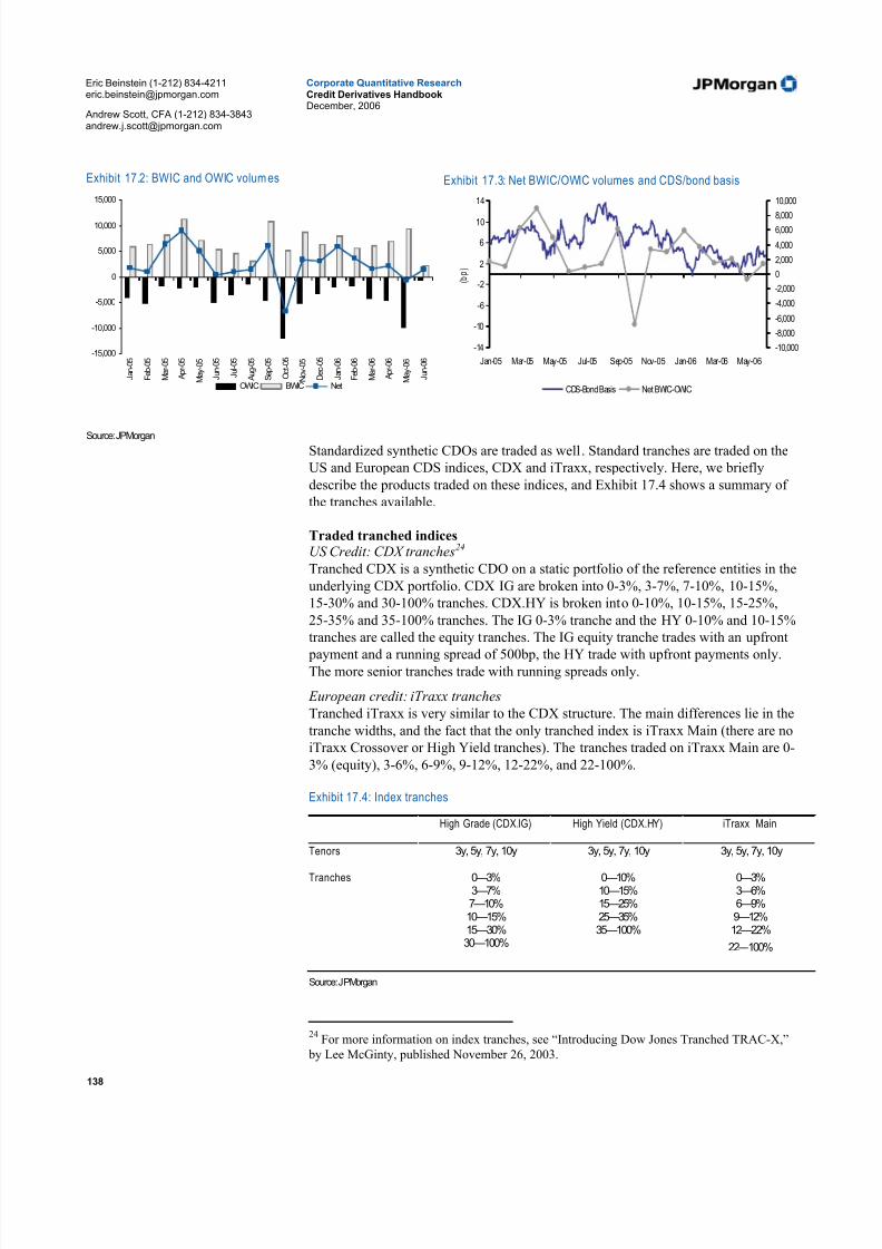
5/10/2018 JPM Credit Derivatives - slidepdf.com
http://slidepdf.com/reader/full/jpm-credit-derivatives-559e0102dc371 138/180
Eric Beinstein (1-212) [email protected]
Andrew Scott, CFA (1-212) [email protected]
Corporate Quantitative ResearchCredit Derivatives HandbookDecember, 2006
138
Exhibit 17.2: BWIC and OWIC volumes Exhibit 17.3: Net BWIC/OWIC volumes and CDS/bond basis
-15,000
-10,000
-5,000
0
5,000
10,000
15,000
J a n - 0 5
F e b - 0 5
M a r - 0 5
A p r - 0 5
M a y - 0 5
J u n - 0 5
J u l - 0 5
A u g - 0 5
S e p - 0 5
O c t - 0 5
N o v - 0 5
D e c - 0 5
J a n - 0 6
F e b - 0 6
M a r - 0 6
A p r - 0 6
M a y - 0 6
J u n - 0 6
OWIC BWIC Net
-14
-10
-6
-2
2
6
10
14
Jan-05 Mar-05 May-05 Jul-05 Sep-05 Nov-05 Jan-06 Mar-06 May-06
( b
p
)
-10,000
-8,000
-6,000
-4,000
-2,000
0
2,000
4,000
6,0008,000
10,000
CDS-Bond Basis Net BWIC-OWIC
Source: JPMorgan
Standardized synthetic CDOs are traded as well. Standard tranches are traded on the
US and European CDS indices, CDX and iTraxx, respectively. Here, we briefly
describe the products traded on these indices, and Exhibit 17.4 shows a summary of
the tranches available.
Traded tranched indicesUS Credit: CDX tranches24
Tranched CDX is a synthetic CDO on a static portfolio of the reference entities in the
underlying CDX portfolio. CDX IG are broken into 0-3%, 3-7%, 7-10%, 10-15%,
15-30% and 30-100% tranches. CDX.HY is broken into 0-10%, 10-15%, 15-25%,
25-35% and 35-100% tranches. The IG 0-3% tranche and the HY 0-10% and 10-15%
tranches are called the equity tranches. The IG equity tranche trades with an upfront
payment and a running spread of 500bp, the HY trade with upfront payments only.The more senior tranches trade with running spreads only.
European credit: iTraxx tranches
Tranched iTraxx is very similar to the CDX structure. The main differences lie in the
tranche widths, and the fact that the only tranched index is iTraxx Main (there are no
iTraxx Crossover or High Yield tranches). The tranches traded on iTraxx Main are 0-
3% (equity), 3-6%, 6-9%, 9-12%, 12-22%, and 22-100%.
Exhibit 17.4: Index tranches
Source: JPMorgan
24For more information on index tranches, see “Introducing Dow Jones Tranched TRAC-X,”
by Lee McGinty, published November 26, 2003.
High Grade (CDX.IG) High Yield (CDX.HY) iTraxx Main
Tenors 3y, 5y, 7y, 10y 3y, 5y, 7y, 10y 3y, 5y, 7y, 10y
Tranches 0—3%3—7%7—10%10—15%15—30%30—100%
0—10%10—15%15—25%25—35%35—100%
0—3%3—6%6—9%9—12%12—22%
22—100%

5/10/2018 JPM Credit Derivatives - slidepdf.com
http://slidepdf.com/reader/full/jpm-credit-derivatives-559e0102dc371 139/180
Eric Beinstein (1-212) [email protected]
Andrew Scott, CFA (1-212) [email protected]
Corporate Quantitative ResearchCredit Derivatives HandbookDecember, 2006
139
Why are synthetic tranches traded?
Tranches have developed into instruments that can provide investors with default
protection, leveraged exposure, hedging tools, and relative value trading
opportunities.
Default protection
Buying protection on an equity tranche provides protection against defaults, up to a
certain limit (as defined by the upper attachment point). This limitation means that
buying default protection via equity tranches may be less expensive than hedging
against defaults using indices.
Leverage
Tranche technology introduces two types of leverage to the risk exposure an investor
can take: leveraged exposure to the risk of portfolio losses, and leveraged exposure to
moves in the spread of the underlying portfolio. In the examples above, we have seen
what happens when portfolio losses exceed the lower attachment point of a tranche.The structure of a tranche, with subordination and a defined tranche width, means
that tranche risk exposure leverages the exposure to portfolio losses. To illustrate
this, consider the seller of protection of the CDX.IG index in comparison to the seller
of the CDX.IG 0-3% equity tranche. If there are no defaults, both sellers of
protection will not bear any losses and will receive spread paid by buyers. However,
in case of one credit event, the seller of the 0-3% tranche will lose 16% of their
notional, while the seller of CDX.IG protection will lose only 0.48% (the
calculations are explained in the next section).
Exhibit 17.5 shows an example of a hypothetical mezzanine 5-10% tranche. As the
illustration shows, the tranche is protected from portfolio losses of less than 5%, but
will begin to experience losses once the portfolio losses exceed this value. Similar to
the equity example above, as the portfolio losses approach the upper attachment point, the tranche loss will be much higher than the portfolio loss. The tranche will
have lost 100% by the time the portfolio has lost only 10%.
Exhibit 17.5: Illustration of tranche reaction to portfolio losses
0% 5% 10% 15% 20% 25% 30%
R e a l i z
e d t r a n c h e l o s s
Realized portfolio loss
0% 5% 10% 15% 20% 25% 30%
R e a l i z
e d t r a n c h e l o s s
Realized portfolio loss
Source: JPMorgan

5/10/2018 JPM Credit Derivatives - slidepdf.com
http://slidepdf.com/reader/full/jpm-credit-derivatives-559e0102dc371 140/180
Eric Beinstein (1-212) [email protected]
Andrew Scott, CFA (1-212) [email protected]
Corporate Quantitative ResearchCredit Derivatives HandbookDecember, 2006
140
Tranche exposure will also provide leverage to spread moves. Since this leverage
refers to a tranche’s sensitivity to underlying spreads, we also use the term " Delta" to
refer to this type of leverage, in line with its usage in options literature. This delta is
often quoted with spreads on the relevant Bloomberg pages (see Exhibit 17.9 below).
With reference to spread moves, the equity tranche is generally the most leveraged of
all the tranches, i.e., the equity tranche usually has the highest Delta. Since the equity
tranche suffers from the first losses in the underlying portfolio, the buyer/seller of
protection of this tranche would pay/receive the highest spread. The likelihood of
other tranches experiencing losses drops as the level of subordination increases.
Therefore, the spreads paid are lower for tranches with more subordination. The
sensitivity to underlying spreads (or Delta) is also lower.
Relative value
From a relative value point of view, tranches often provide higher spread for rating
when compared with other credit investments. Exhibit 17.6 shows an indication of
spread for rating across credit instruments. Tranches themselves are not rated by therating agencies, but indicative ratings can be calculated based on the rating agency’s
methodologies. Exhibit 17.7 shows JPMorgan’s calculations of the ratings that S&P
might assign to the tranches in iTraxx Main Series 6.
Exhibit 17.6: Spread-for-rating comparison
¹ Especially in structured synthetic corporate credit risk, spreads depend on factors such as leverage (tranche width) and spread for
rating in the underlying asset pool. A wide range of spreads can therefore be achieved for the same rating.
Exhibit 17.7: Likely iTraxx Main Series 6 tranche ratin gs (using S&P's tranche evaluator 3.0)
Sources: JPMorgan, S&P
HedgingThe synthetic tranche has become useful as a hedge against portfolio losses or spread
moves in the underlying portfolio, particularly on bespoke portfolios. From an
outright trade perspective, investors with default risk against a portfolio of credits
can now use tranches on bespoke portfolios to hedge against precisely the names in
their portfolio. These hedges may be less expensive than using indices or options.
And as tranches on the indices are more and more liquid, they have caught the
attention of speculative traders, bank proprietary desks and hedge funds that may be
interested in the risk on the other side of the hedge.
Delta refers to the sensitivity of a
tranche to move in the spread of
the underlying portfolio
Ratings Underlying Indicative spreadAAA RMBS 11bp
AAA CMBA 19bp
AAA iTraxx Series 6, 6-9% standard tranche¹ 22bp
AAA Managed synthetic CSO, higher levered¹ 30bp
AAA Corporate bonds <5bp
5y 7y 10y0—3% - - -
3—6% BBB- BB B
6—9% AAA AA BBB
9—12% AAA AAA AAA
12—22% AAA AAA AAA
22—100% SS SS SS

5/10/2018 JPM Credit Derivatives - slidepdf.com
http://slidepdf.com/reader/full/jpm-credit-derivatives-559e0102dc371 141/180
Eric Beinstein (1-212) [email protected]
Andrew Scott, CFA (1-212) [email protected]
Corporate Quantitative ResearchCredit Derivatives HandbookDecember, 2006
141
The mechanics of trading tranche protection
The tranched index products create a standardized, liquid, and transparent instrument
to trade defined amounts of credit risk. Now, we show in more detail just how these
instruments manage to access these specific slices of risk.
Assume the 0-3% tranche of the 5Y DJ NA.CDX.IG is trading at 500bp (for
simplification, assume there is no upfront payment). The tranche exposes investors to
the first 3% of losses on the CDX.IG portfolio. The buyer of protection will pay
500bp annually on the outstanding notional while the seller of protection will receive
500bp annually.
In case of no defaults
If there are no defaults on the portfolio of 125 names over the 5-year maturity, the
buyer/seller of protection will pay/receive 500bp per annum on the full notional, over
five years.
In case of defaults
Assume a credit event occurs after two years. This would trigger settlement cash-
flows for buyers and sellers of protection of the 0-3% tranche. Assuming a recovery
rate of 40%, this equates to a 60% loss on the credit, or a 0.48% loss on the 125-
credit portfolio of the CDX.IG (1/125 x 60% = 0.48%). The seller of protection of
the 0-3% tranche would pay the buyer of protection 16% (0.48%/3%) of the notional.
After this point, the coupon would remain at 500bp, but on a reduced notional of
84% of the original value.
The credit event affects the attachment points of each tranche, as the subordination of
each tranche is changed. The upper attachment point of the 0-3% tranche becomes
2.52%, in our example: 3% - (1/125 x 60%) = 3% - 0.48% = 2.52%. The lower and
upper attachment points of the mezzanine and senior tranches are each reduced by0.48%, while the width of the tranche and the notional remains the same. On the 30 -
100%, or super senior tranche, both the attachment points and notional are reduced.
The notional is reduced because the “fate” of one of the credits has been decided and
the recovered amount on the default name can no longer be "lost.” In our example,
the notional is reduced by (1/125 x 40%). In essence, the credit event affects the
“bookends” of the most junior and most senior tranches, reducing the notional on the
junior tranche by (1/125) times (percent lost on the credit), and (1/125) times
(percent recovered on the credit) for the senior tranche.
If there were seven defaults, all recovering at 40%, the total loss on the CDX.IG
portfolio would be 3.36%. The first 3% of the 3.36% loss would cause the seller of
protection of the 0-3% tranche to lose the entire notional they put at risk. They would
have no more exposure to further credit events. Similarly, the buyer of protection on
this tranche would earn the full notional at risk and would no longer have to pay the
spread. The remaining 0.36% loss would trigger the settlement cash flows between
the buyers and sellers of protection of the 3-7% tranche.
Cashflow structures
Tranche cashflows can be structured in three ways: all running spread, all upfront, or
upfront + running spread. In an all running spread structure, which is typical for
mezzanine tranches, the spread is fixed for the life of the trade. On an all-upfront
basis, investors pay/receive an initial payment (the “upfront premium") and
receive/pay for the loss contingent on defaults as the defaults occur. The upfront

5/10/2018 JPM Credit Derivatives - slidepdf.com
http://slidepdf.com/reader/full/jpm-credit-derivatives-559e0102dc371 142/180
Eric Beinstein (1-212) [email protected]
Andrew Scott, CFA (1-212) [email protected]
Corporate Quantitative ResearchCredit Derivatives HandbookDecember, 2006
142
premium is equal to the present value of the expected loss. Equity tranches are often
traded as upfront + running spread, where the running spread is kept constant at
500bp, and the initial payment is calculated accordingly.
The role of correlation
What is the correlation measure?
The correlation we speak of is the correlation as implied by market spreads. An
implied correlation number describes the expected contagion of default among
portfolio entities. In other words, when speaking of “correlation trading" or “implied
correlations,” we really speak about the market’s view on how correlated the CDS
portfolio is, as implied by the spreads traded in the market.
The effect of correlation on tranche valuations
As a tranche references the amount of losses in the underlying portfolio, the
correlation of the behavior of the reference entities in the event of portfolio losses is
central to the value of a tranche. An increase in mezzanine and senior tranche spreads means that buying protection on these tranches will be more expensive. This
indicates the market expects defaults in the portfolio should affect the more senior
tranches, or that defaults are likely to be correlated. As a result, spreads in the equity
tranches will respond by moving tighter . We would see the opposite occur with a
decrease in correlation.
The example above illustrates the relationship among tranche spreads, which can be
thought of in analogy to the law of conservation of energy. In tranched portfolios, we
see a "conservation of risk." The capital structure on a given portfolio has a certain
amount of risk, which tranches divide into components. The possibility of arbitrage
between the portfolio and the tranches will keep the "sum of tranche risk" balanced
with the risk of the whole reference portfolio. Assuming the spread of the underlying
portfolio or index remains constant (which means the overall risk in the underlying portfolio remains constant), supply and demand pressures may redistribute risk from
one tranche into another, but the overall amount of risk can not change. In other
words, given that portfolio spread remains constant, a change in the spread of one
tranche must result in a respective change in the spread of another tranche
somewhere else in the capital structure.
Exhibit 17.8 illustrates this concept. With correlation at 10%, the portfolio loss
distribution shows that portfolio losses are likely to remain confined below the more
senior tranches. In other words, not much subordination is required to provide
protection from portfolio losses. But, when correlation increases to 40%, the
portfolio loss distribution encroaches on the more senior tranches and more
subordination would be required for the same amount of protection. The extreme
case, correlation of 100% across the portfolio, would result in one default within the
portfolio causing the entire portfolio to default. In this case, the spreads across the
tranches would all be equal.

5/10/2018 JPM Credit Derivatives - slidepdf.com
http://slidepdf.com/reader/full/jpm-credit-derivatives-559e0102dc371 143/180
Eric Beinstein (1-212) [email protected]
Andrew Scott, CFA (1-212) [email protected]
Corporate Quantitative ResearchCredit Derivatives HandbookDecember, 2006
143
Exhibit 17.8: Illustration: Impact of a change in base correlation
P r o b a b i l i t y
Portfolio loss
0-3% 3-6% 6-9% 22-100%
Loss distribution 2, correlation 40%
Loss distribution 1, correlation 10%
Lossdistribution 3,
correlation100%
………
P r o b a b i l i t y
Portfolio loss
0-3% 3-6% 6-9% 22-100%
Loss distribution 2, correlation 40%
Loss distribution 1, correlation 10%
Lossdistribution 3,
correlation100%
………
Source: JPMorgan
Correlation skew
Although in theory there should be one number that describes the correlation across
the single names in the portfolio, we can measure a unique “base correlation” at each
attachment point. As demand will pull spreads in varying degrees for each tranche,
there will be a “correlation skew” for the portfolio. Correlation skew also results
from the fact that correlation is an implied number, based on models that translate
spread moves into sentiment on correlation. Hence both the technical moves in
relative tranche spreads, and the weaknesses of the models themselves, result in arange of implied correlations along the capital structure.
Pricing tranches
Having looked at the mechanics and some of the drivers of tranche valuation, we turn
now to the practicalities of pricing.
Quoted prices
Bloomberg screens like the one shown in Exhibit 17.9 show bid/offer spreads (or
upfront cost for equity tranches) for the different tranches traded on the indices.
JPTX <Go> will take Bloomberg users to the menu page to view JPMorgan prices on
the various indices available.

5/10/2018 JPM Credit Derivatives - slidepdf.com
http://slidepdf.com/reader/full/jpm-credit-derivatives-559e0102dc371 144/180
Eric Beinstein (1-212) [email protected]
Andrew Scott, CFA (1-212) [email protected]
Corporate Quantitative ResearchCredit Derivatives HandbookDecember, 2006
144
Exhibit 17.9: Sample tranched index pricing page
Source: JPMorgan, Bloomberg
Marking-to-market
Similar to CDS contracts, tranches are marked to market using the risky present
value of the change in spread. The Risky Annuity is the factor by which we can
multiply the change in spreads to compute this present value. In essence, it represents
the present value per basis point of spread paid over the life of the contract, assuming
the relevant coupon dates and survival probabilities.
Hence, we define the mark-to-market (MtM) as
NotionalAnnuityRisky)(MtM i1i)1,-(i ⋅⋅−=− ii S S
where Si represents the spread level at time i, and
( )4 4 4 4 34 4 4 4 214 4 34 4 21
lossagivenowedaccrualaverage
1
1
survivaloncontingentfee
1
i2
AnnuityRisky ∑∑=
−
=
⋅−⋅∆
+⋅⋅∆=
n
i
iiii
n
i
iii DF Ps Ps DF Ps
JPMorgan's Heterogeneous Gaussian Copula Model25
(“HGC Model”)
JPMorgan has developed this model for pricing tranche risk, which can be used tomark-to-market tranche positions, as well as to measure the sensitivities of tranche
spreads. As we have seen, correlation is relevant to tranche valuations as it
determines the main driver of a tranche spread: the expected loss of the tranche.
There are a number of ways of calculating the expected loss of a tranche. In our enhanced tranche pricer, we use a Gaussian copula pricing methodology that can
25For more information on the HGC Model and tranche sensitivities, see Enhancing our
Framework for index tranche analysis, Dirk Muench, September 2005 and Using JPMorgan’s
Framework for Tranche Analysis , Dirk Muench, May 2006.
Risky Duration (DV01) vs.Risky Annuity
These are often used
interchangeably, but for the
record, there is a difference.
Risky Duration (DV01) is the
change in mark-to-market of a
tranche contract for a 1bp
parallel shift in spreads
Risky Annuity is the present
value of a 1bp annuity as defined
here
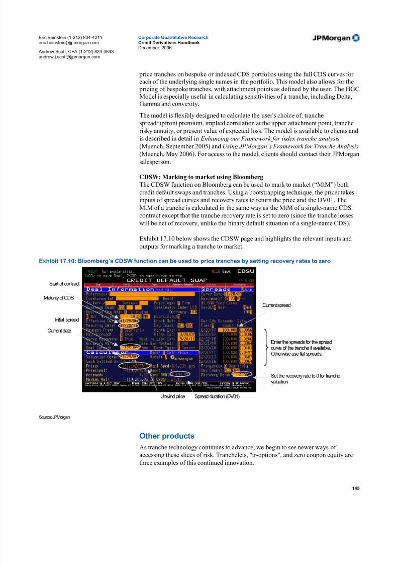
5/10/2018 JPM Credit Derivatives - slidepdf.com
http://slidepdf.com/reader/full/jpm-credit-derivatives-559e0102dc371 145/180
Eric Beinstein (1-212) [email protected]
Andrew Scott, CFA (1-212) [email protected]
Corporate Quantitative ResearchCredit Derivatives HandbookDecember, 2006
145
price tranches on bespoke or indexed CDS portfolios using the full CDS curves for each of the underlying single names in the portfolio. This model also allows for the
pricing of bespoke tranches, with attachment points as defined by the user. The HGC
Model is especially useful in calculating sensitivities of a tranche, including Delta,Gamma and convexity.
The model is flexibly designed to calculate the user's choice of: tranche
spread/upfront premium, implied correlation at the upper attachment point, tranche
risky annuity, or present value of expected loss. The model is available to clients and
is described in detail in Enhancing our Framework for index tranche analysis
(Muench, September 2005) and Using JPMorgan’s Framework for Tranche Analysis
(Muench, May 2006). For access to the model, clients should contact their JPMorgan
salesperson.
CDSW: Marking to market using Bloomberg
The CDSW function on Bloomberg can be used to mark to market (“MtM”) both
credit default swaps and tranches. Using a bootstrapping technique, the pricer takes
inputs of spread curves and recovery rates to return the price and the DV01. The
MtM of a tranche is calculated in the same way as the MtM of a single-name CDS
contract except that the tranche recovery rate is set to zero (since the tranche losses
will be net of recovery, unlike the binary default situation of a single-name CDS).
Exhibit 17.10 below shows the CDSW page and highlights the relevant inputs and
outputs for marking a tranche to market.
Exhibit 17.10: Bloomberg’s CDSW function can be used to price tranches by setting recovery rates to zero
Source: JPMorgan
Other products
As tranche technology continues to advance, we begin to see newer ways of
accessing these slices of risk. Tranchelets, "tr-options", and zero coupon equity are
three examples of this continued innovation.
Current spread
Current date
Maturity of CDS
Unwind price Spread duration (DV01)
Enter the spreads for the spreadcurve of the tranche if available.Otherwise use flat spreads.
Set the recovery rate to 0 for tranchevaluation
Start of contract
Initial spread
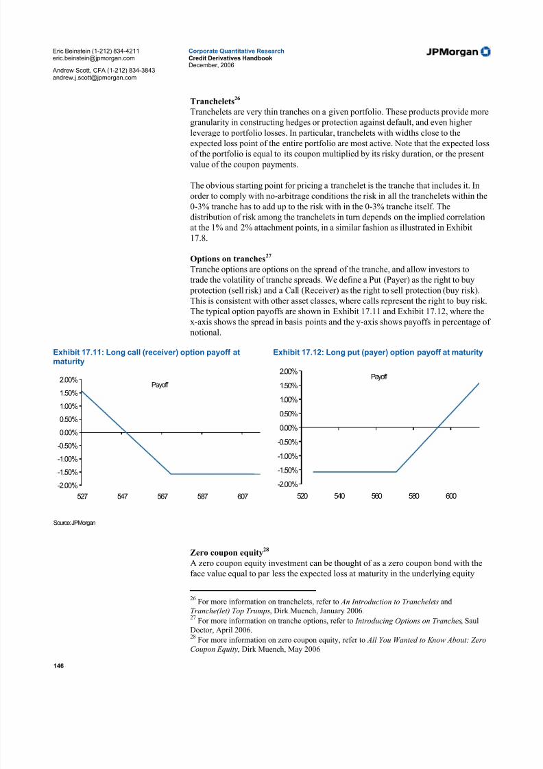
5/10/2018 JPM Credit Derivatives - slidepdf.com
http://slidepdf.com/reader/full/jpm-credit-derivatives-559e0102dc371 146/180
Eric Beinstein (1-212) [email protected]
Andrew Scott, CFA (1-212) [email protected]
Corporate Quantitative ResearchCredit Derivatives HandbookDecember, 2006
146
Tranchelets26
Tranchelets are very thin tranches on a given portfolio. These products provide more
granularity in constructing hedges or protection against default, and even higher
leverage to portfolio losses. In particular, tranchelets with widths close to theexpected loss point of the entire portfolio are most active. Note that the expected loss
of the portfolio is equal to its coupon multiplied by its risky duration, or the present
value of the coupon payments.
The obvious starting point for pricing a tranchelet is the tranche that includes it. In
order to comply with no-arbitrage conditions the risk in all the tranchelets within the
0-3% tranche has to add up to the risk with in the 0-3% tranche itself. The
distribution of risk among the tranchelets in turn depends on the implied correlation
at the 1% and 2% attachment points, in a similar fashion as illustrated in Exhibit
17.8.
Options on tranches27
Tranche options are options on the spread of the tranche, and allow investors totrade the volatility of tranche spreads. We define a Put (Payer) as the right to buy
protection (sell risk) and a Call (Receiver) as the right to sell protection (buy risk).
This is consistent with other asset classes, where calls represent the right to buy risk.
The typical option payoffs are shown in Exhibit 17.11 and Exhibit 17.12, where the
x-axis shows the spread in basis points and the y-axis shows payoffs in percentage of
notional.
Exhibit 17.11: Long call (receiver) option payoff atmaturity
-2.00%
-1.50%
-1.00%
-0.50%
0.00%
0.50%
1.00%
1.50%
2.00%
527 547 567 587 607
Payoff
Exhibit 17.12: Long put (payer) option payoff at maturity
-2.00%
-1.50%
-1.00%
-0.50%
0.00%
0.50%
1.00%
1.50%
2.00%
520 540 560 580 600
Payoff
Source: JPMorgan
Zero coupon equity28
A zero coupon equity investment can be thought of as a zero coupon bond with the
face value equal to par less the expected loss at maturity in the underlying equity
26For more information on tranchelets, refer to An Introduction to Tranchelets and
Tranche(let) Top Trumps, Dirk Muench, January 2006.27
For more information on tranche options, refer to Introducing Options on Tranches, SaulDoctor, April 2006.28
For more information on zero coupon equity, refer to All You Wanted to Know About: Zero
Coupon Equity, Dirk Muench, May 2006

5/10/2018 JPM Credit Derivatives - slidepdf.com
http://slidepdf.com/reader/full/jpm-credit-derivatives-559e0102dc371 147/180
Eric Beinstein (1-212) [email protected]
Andrew Scott, CFA (1-212) [email protected]
Corporate Quantitative ResearchCredit Derivatives HandbookDecember, 2006
147
tranche. There are just two cash flows taking place for an investor in a zero coupon
bond: one at trade inception, and one at maturity (or when the investment is unwound
before maturity). The size of the cash flow at maturity depends only on the notional
loss on the underlying tranche - it does not depend on when this loss occurred. Thestructure often provides a high internal rate of return with a payout on a certain date,
which can be more attractive than a standard tranche contract where the date of
cashflows is uncertain (i.e. occurs at the time of default). The high return comes
from the fact that the initial payment assumes an expected loss, which is likely to be
higher than the realized loss, thus lowering the initial cash flow.
100 – Notional loss on tra
Present value of (100 – Notional loss on tranche)
T = 0
T = Maturity
100 – Notional loss on tra
Present value of (100 – Notional loss on tranche)
T = 0
T = Maturity

5/10/2018 JPM Credit Derivatives - slidepdf.com
http://slidepdf.com/reader/full/jpm-credit-derivatives-559e0102dc371 148/180
Eric Beinstein (1-212) [email protected]
Andrew Scott, CFA (1-212) [email protected]
Corporate Quantitative ResearchCredit Derivatives HandbookDecember, 2006
148

5/10/2018 JPM Credit Derivatives - slidepdf.com
http://slidepdf.com/reader/full/jpm-credit-derivatives-559e0102dc371 149/180
Eric Beinstein (1-212) [email protected]
Andrew Scott, CFA (1-212) [email protected]
Corporate Quantitative ResearchCredit Derivatives HandbookDecember, 2006
149
Part IV: Other CDS products
18. Loan CDS..........................................................................................................150
Overview ...........................................................................................................150Comparing CDS contracts across asset classes .................................................150Similarities and differences between CDS and LCDS.......................................151Participants ........................................................................................................154Settlement following a credit event ...................................................................154Modifications to LSTA transfer documents ......................................................156Rating agency approach to LCDS in structured credit ......................................156Spread relationship between loans and LCDS...................................................157
19. Preferred CDS..................................................................................................158
Overview ...........................................................................................................158Preferred stock CDS contracts differ from the standard CDS contract..............158PCDS versus CDS .............................................................................................160
Overview of preferred stock issuance and market.............................................160
20. Profiting from views on recovery rates ..........................................................162
Recovery Rate Lock ..........................................................................................162Digital Default Swaps........................................................................................167
21. Other credit default swap products................................................................168Credit linked notes.............................................................................................168Constant maturity credit default swaps and credit spread swaps ......................169First-to-default baskets ......................................................................................170

5/10/2018 JPM Credit Derivatives - slidepdf.com
http://slidepdf.com/reader/full/jpm-credit-derivatives-559e0102dc371 150/180
Eric Beinstein (1-212) [email protected]
Andrew Scott, CFA (1-212) [email protected]
Corporate Quantitative ResearchCredit Derivatives HandbookDecember, 2006
150
18. Loan CDS
Overview
The emergence of a standardized secured loan CDS (LCDS29) market is a major development in the evolution of the loan market. Loans have historically been along-only cash asset, with little or no ability for participants to go short risk or takeon risk synthetically.
LCDS allows investors to take advantage of benefits and risks similar to thoseavailable to investors in standard CDS. These include:
• The ability to implement a bullish view (sell LCDS protection) without
having to access the primary or secondary market for cash loans. The
ability to create levered portfolios of secured risk.
• The ability to hedge or implement bearish views on loans (buy LCDS protection) and be short risk in what has traditionally been a long-only
market.
• The ability to trade cross-asset views such as a view on the senior debt
spread versus loan spread.
• The ability to implement curve shape positions and views once the market
develops and a LCDS spread curve becomes available.
LCDS contracts are based on the standard corporate CDS contract, with severalmodifications to address the unique nature of the loan market. We discuss thesedifferences, along with modifications made to LSTA documents, herein. Note that
the actual terms of a LCDS transaction are defined by the confirmation of thattransaction only, and this research note forms no part of that document.
Comparing CDS contracts across asset classes
Exhibit 18.1 compares CDS contracts for standard corporate CDS, Loan CDS,Preferred CDS, and Asset Backed CDS.
29For more information on LCDS, refer to “Introducing Credit Default Swaps on Secured
Loands (LCDS)” by Eric Beinstein and Ben Graves, published March 30, 2006.

5/10/2018 JPM Credit Derivatives - slidepdf.com
http://slidepdf.com/reader/full/jpm-credit-derivatives-559e0102dc371 151/180
Eric Beinstein (1-212) [email protected]
Andrew Scott, CFA (1-212) [email protected]
Corporate Quantitative ResearchCredit Derivatives HandbookDecember, 2006
151
Exhibit 18.1: Comparison of CDS across diff erent asset classes
Corporate CDS
(CDS)
Loan CDS
(LCDS)
Preferred CDS
(PCDS)
Asset Backed CDS
(ABCDS)
Reference
Obligation
Obligation of the issuer Syndicated secured loan of
the issuer
Obligation of the issuer itself
or a related preferred issuer
Specific security issued by
the Reference Entity
Credit events Bankruptcy, failure to pay,
restructuring (for HG only)
Bankruptcy, failure to pay Bankruptcy, failure to pay,
restructuring, and deferral on
the payment of a preferred
stock dividend
Principal shortfall and
writedown
Deliverable
obligations
Bonds and loans Syndicated Secured loans
only
Preferred securities. Also
bonds and loans in most
cases.
Asset backed security,
CUSIP specific
Notional amount Par amount Par amount Par amount Amortization mirrors the
underlying bonds
Contract size Typically $5-20 million Typically $2-$5 million Typically $5 million Typically $5-10 million
Settlement Physical
(with cash option)
Physical or Partial Cash
(with cash option)
Physical
(with cash option)
Pay as you go
(with physical settlement
option)
Term 5 - 10 years 5 years currently 5 years currently Equal to the longest maturity
asset in the pool. Roughly
30 years for mortgages.
Additional
Information
“Credit Derivatives: A Primer,”
JPMorgan, January 2005.
“Introducing CDS on Secured
Loans,” JPMorgan, March
2006.
“Introducing CDS on Preferred
Stock,” JPMorgan, March
2006
“Single Name CDS of ABS,”
JPMorgan, March 2005
Source: JPMorgan
Similarities and differences between CDS and LCDS
Like standard corporate CDS, LCDS credit events include bankruptcy and failure to pay. Note that the failure to pay credit events applies to borrowed money, althoughthe deliverables are syndicated secured loans only. This means that a failure to payon the senior unsecured bonds, for example, would trigger a credit event even if theloans were paid as due (assuming they are the same borrower).
With regard to restructuring, LCDS contracts on US high yield issuers will followthe convention for standard corporate CDS. This will typically mean that the LCDS
contract will exclude restructuring, since most US corporate HY CDS contractsexclude restructuring. For example, if a term loan is restructured with new covenantsand a higher spread, the LCDS contract will remain outstanding with no change incoupon exchanged between existing counterparties.
LCDS Reference Obligation: syndicated secured loan
One difference between an LCDS and CDS contract is the level of the capitalstructure each contract “points” to. Namely, the reference obligation of most CDScontracts is a Senior Unsecured bond, while the reference obligation of a LCDScontract must be a syndicated secured loan. The loan may be a first, second or thirdlien note, but it must be secured.

5/10/2018 JPM Credit Derivatives - slidepdf.com
http://slidepdf.com/reader/full/jpm-credit-derivatives-559e0102dc371 152/180
Eric Beinstein (1-212) [email protected]
Andrew Scott, CFA (1-212) [email protected]
Corporate Quantitative ResearchCredit Derivatives HandbookDecember, 2006
152
Exhibit 18.2: Structural considerations – loans versus bonds
Traditional syndicated loans Second lien loans High yield bonds
Size: Any amount Any amount; typically <$300mm $100mm–125mm minimum
Security: First-lien priority (assets and stock) Second–lien priority (assets and stock) Unsecured or subordinated,sometimes secured
Maturity: Up to 5–7 years Typically 5–7 years Typically 7–10 years
Interest rates: Floating Floating Fixed
Call flexibility: Callable generally at par Flexible, near–term call protection Typically non–callable for 4–5 years
Amortization: Yes, typically back–ended Yes, typically back–ended None
Covenants: Maintenance–based, more restrictive
than public or private notes
Bond–like with the exception of a total
leverage maintenance covenant set
wide of traditional bank covenant
Full, but unrestrictive, set of
incurrence–based financial covenants
SEC filing: None None Registration rights, generally within
180 days in a 144A offering
Disclosure: Detailed (including projections);bifurcated between public and private
investors
Detailed (including projections);bifurcated between public and private
investors
Public disclosure; no projections Reg.FD
Ratings: Moody’s and S&P Moody’s and S&P Moody’s and S&P
Syndication/roadshow timing: 4–6 Weeks Potential investor
meetings/ conference call
4–6 Weeks Investor meeting likely 6–8 weeks Recommended 5–7 day
roadshow
Investors Commercial banks, mutual funds,
insurance companies, prime funds,
structure vehicles, CLOs
Hedge funds, prime rate funds,
insurance companies, high yield
crossover accounts, CLOs and CDOs
Mutual funds, insurance companies,
money managers, bond funds, hedge
funds
Ability to alter terms High Medium Low
Source: JPMorgan
Investment grade-rated companies generally have loans and bonds that are pari passu, or both having senior unsecured claims with equal rights to payment. Sub-investment grade companies, however, tend to have loans that are senior secured and
bonds that are senior unsecured and senior subordinated. In the case of default, thismeans that the loans will have first priority on any recovery available to the debt-holders. As a result, the implied recovery rate on loans is much higher than for the
bonds, and the risk to principal is therefore much lower for loans (Exhibit 18.3).
Because loans issued by investment grade-rated companies are generally senior unsecured claims, the vast majority of LCDS contracts will be limited to high yieldissuers.

5/10/2018 JPM Credit Derivatives - slidepdf.com
http://slidepdf.com/reader/full/jpm-credit-derivatives-559e0102dc371 153/180
Eric Beinstein (1-212) [email protected]
Andrew Scott, CFA (1-212) [email protected]
Corporate Quantitative ResearchCredit Derivatives HandbookDecember, 2006
153
Exhibit 18.3: Recovery rates by priority
0%
10%
20%
30%
40%
50%
60%
70%
80%
Secured Bank
Loans
Sr. Secured
Bonds
Sr. Unsecured
Bonds
Sr. Subordinated
Bonds
Preferred Stock
Overall (1990–2005) 2000–2005
Source: Moody’s Investors Service
A list of secured loan reference obligations and their priority will be publishedregularly by a third party. Contents of the list will be voted on by dealers on aregular basis.
Cancel-ability - the termination of an LCDS contract
A second difference between CDS and LCDS is that an LCDS contract is cancelled if there are no deliverable reference obligations outstanding, in other words, a senior secured loan must be outstanding. Recall that a CDS contract is not cancelled, evenif the company tenders for all outstanding debt. The LCDS contract is different.
LCDS contracts remain outstanding if the reference loan is refinanced or replacedwith another secured loan. If the original reference loan no longer exists for anyreason, a replacement obligation can be selected. The replacement must be pari
passu to the previous reference loan or, if none exists, higher in priority than the previous reference loan. For example, if an issuer refinances their existing loans andreissues new loans, the old LCDS contract will reference the new loans and theLCDS coupon will remain unchanged.
If a replacement cannot be found (i.e. no secured loans exist), or if the replacement isof a higher priority, either party has the option to terminate the contract. There is nounwind fee paid, the LCDS contract is simply terminated.
Either the buyer or seller can dispute the security of a loan and whether it is an
acceptable reference, substitute, or deliverable obligation. The dispute is resolvedvia a poll of specified dealers as to whether the loan is “syndicated secured.” To besyndicated secured, the loan must be issued under a syndicated loan agreement andtrade as a loan of the designated priority in the secondary market. Note that thisdefinition does not require a legal opinion as to the security and priority of the loan,
but rather requires consensus among market participants as to how the loan trades instandard market practice.

5/10/2018 JPM Credit Derivatives - slidepdf.com
http://slidepdf.com/reader/full/jpm-credit-derivatives-559e0102dc371 154/180
Eric Beinstein (1-212) [email protected]
Andrew Scott, CFA (1-212) [email protected]
Corporate Quantitative ResearchCredit Derivatives HandbookDecember, 2006
154
Participants
As in standard CDS, banks and hedge funds are the most active users of LCDS.Participants include:
Banks and other lenders: LCDS provides an attractive opportunity for discretehedging as an alternative to selling cash loans. LCDS also serves as an alternative to
proxy hedging loan exposure in the bond or standard corporate CDS market – ahedge which introduces spread correlation, recovery, basis, and other risks.
Total return funds: Total return funds can use LCDS to effectively create levered portfolios of secured risk. We also anticipate selective positioning on spreadwidening or protective single-name hedging.
Structured credit vehicles: In the current market, where allocations to cash loanscontinue to be squeezed by excessive demand, we expect cash CLOs to sell
protection (long risk) as an alternative means to access the loan market. LCDS alsohelps CLOs avoid high dollar prices in cash loans trading in the secondary market(high dollar prices decrease initial overcollateralization ratios), and some newstructures are already incorporating synthetic buckets. LCDS also provides the
potential for fully synthetic managed, bespoke, and index-tranched trades.
Structured credit investors: LCDS gives investors the ability to dynamically hedgesingle loans in cash CLOs or synthetic structured credit portfolios.
Capital Structure investors: Capital structure investors can express views onsecured loans in relation to other securities including unsecured bonds, preferredstock, or common stock. Typical trades include selling LCDS protection (long risk)versus short a subordinate security (in cash or derivative form) or buying LCDS
protection (short risk) vs. long a subordinate security (in cash or derivative form).
Settlement following a credit event
Settlement Timing
Like in traditional CDS contracts, the protection buyer has 30 days following a creditevent notice to declare their intent to settle physically by delivering a notice of
physical settlement (NOPS). The NOPS Fixing Date is set at 3 business days after the notice of physical settlement is delivered. As soon as practicable after the NOPSFixing Date, the protection buyer must deliver all necessary documents to effect
physical settlement. Upon receipt of these documents, the protection seller has 3 business days to execute and return the documents.
What loans are deliverable if there is a credit event?
After a credit event, loans on the secured list, or other loans that trade as syndicated
secured of equal or higher priority, are deliverable. Term loans, revolving loans, andmulti-currency loans are all deliverable.
In the case of revolvers, a seller of protection who is delivered revolving loans isliable for any future draws on the revolver, although in nearly all cases30 the ability todraw on a revolver is eliminated upon a default.
30One exception may be outstanding letters of credit, which may in some cases may be drawn.
This is relatively rare.
5/10/2018 JPM Credit Derivatives - slidepdf.com
http://slidepdf.com/reader/full/jpm-credit-derivatives-559e0102dc371 155/180
Eric Beinstein (1-212) [email protected]
Andrew Scott, CFA (1-212) [email protected]
Corporate Quantitative ResearchCredit Derivatives HandbookDecember, 2006
155
Loans trading above par after a credit eventIn some cases, cash loans may trade above par after a credit event. The protection
buyer, however, will not be forced to realize a loss on the difference between par andthe loan price.31
Settlement Mechanics
Like traditional CDS contracts, LCDS documents call for physical settlement,although (like corporate CDS) they do not preclude bilateral settlement agreementsor participation in any cash settlement or netting protocols that may be developed,and we anticipate that a significant proportion of contracts will be cash settled.Physical settlement is governed by the documents customarily used by the LoanSyndications and Trading Association (LSTA) that are current at the notice of
physical settlement fixing date, subject to the modifications discussed in thefollowing section of this note. The physical settlement process calls for settlement
by:
Assignment: In an assignment, the protection seller becomes a direct signatory to the
loan agreement. Assignments typically require the consent of the borrower andagent.
Participation: If the loan cannot be transferred to the seller via assignment due to lack of necessary consent or other failure to meet requirements under the creditagreement, settlement may occur by participation. In a participation, the protectionseller takes a participating interest in the existing lender’s commitment, with the
protection buyer remaining the title holder of, and lender under, the loan.
Settlement may also occur by subparticipation (the protection buyer does not own theloan, but holds a participation from another party). In this scenario, the protectionseller will receive a participation, and will receive payments only to the extent the
protection buyer receives payment from his upstream counterparty. A protection
buyer is not stepping up if he does not receive payments from the grantor of theoriginal participation. Accordingly, the protection seller is taking credit risk of morethan just the protection buyer .
Cash Settlement: If settlement cannot be completed due to failure to meetrequirements under the credit agreement (e.g. lack of necessary consent), or if theseller of protection elects to cash settle, settlement may occur by partial cashsettlement. The cash settlement amount will be the difference between 100% and theloan price as determined from dealer quotations, and cannot be negative (i.e. the
buyer does not pay the seller even if the loan trades above par following a creditevent).
31 In this situation, a protection buyer could determine not to deliver the notice of physical settlement and
the transaction will terminate. In physical settlement, the protection buyer would not deliver the loan, notreceive par, and would owe accrued up to the event date. There is also language in the LCDS docs thatstates that in partial cash settlement, the protection buyer does not pay the protection seller even if the loantrades above par following a credit event.

5/10/2018 JPM Credit Derivatives - slidepdf.com
http://slidepdf.com/reader/full/jpm-credit-derivatives-559e0102dc371 156/180
Eric Beinstein (1-212) [email protected]
Andrew Scott, CFA (1-212) [email protected]
Corporate Quantitative ResearchCredit Derivatives HandbookDecember, 2006
156
Modifications to LSTA transfer documents
Market Standard Indemnity
Unlike standard cash loan settlement, loans delivered under LCDS contracts are physically transferred using the LSTA Purchase and Sale Agreement (PSA) templatethat is standard at the notice of physical settlement fixing date, without any credit-specific negotiation or amendments. The reason for using the template rather than a negotiated agreement is to expedite the settlement of a potentially large number of contracts after a credit event.
Although the template is used without negotiation, buyers and sellers recapture theeconomics of “standard market practice” documents with the Market StandardIndemnity. The protection buyer agrees to indemnify the protection seller for anyloss suffered as a result of inconsistency between the documents actually used for
physical transfer and the documents reflecting “standard market practice” for thespecific loan at the time of transfer.
For example, consider a protection seller who is physically delivered a loan under the
PSA template. If at some time in the future the protection seller realizes a loss (e.g.receives fewer payments or less favorable treatment) relative to lenders with marketstandard documents, the protection seller can recoup this loss from the protection
buyer (including via litigation, if necessary) using the Market Standard Indemnity.
Rating agency approach to LCDS in structured credit
Rating agency treatment of LCDS is critical to structured credit investors, as itinfluences the subordination required to achieve a desired tranche rating. Althoughthe rating agency approach to LCDS has not yet been finalized, we briefly discussthe most relevant issues for both investors and the agencies.
Assumed default probability: It is possible for a company to default on its bonds but
not its loans. For rating agencies that maintain separate secured and unsecureddefault probabilities, it is questionable which is the “correct” default probability for LCDS. Since the LCDS Failure to Pay credit event applies to all borrowed money(including both bonds and loans), some rating agencies may apply the relativelyhigher unsecured default rate to LCDS.
Assumed recovery rate: Rating agencies will need to determine what recovery rate ismost appropriate for LCDS. They will likely look to the soundness of the contract
provisions for deliverable obligations and replacement obligations to determinewhether the their first lien recovery rate is most appropriate versus using second lienrecovery rates or a haircut to first lien recovery rates.
Cheapest to deliver haircut: Some rating agencies apply a “cheapest to deliver”
haircut to recovery rates on standard corporate CDS to compensate for the protectionseller's option to deliver the bond or loan trading at the lowest dollar price followinga credit event. We would expect a similar haircut to be applied to LCDS, althoughthe magnitude is not yet clear.
5/10/2018 JPM Credit Derivatives - slidepdf.com
http://slidepdf.com/reader/full/jpm-credit-derivatives-559e0102dc371 157/180
Eric Beinstein (1-212) [email protected]
Andrew Scott, CFA (1-212) [email protected]
Corporate Quantitative ResearchCredit Derivatives HandbookDecember, 2006
157
Spread relationship between loans and LCDS
The spread relationship between loans and LCDS is dynamic and depends on theinterplay of both technical and structural factors. We discuss these factors below,including our rationale for why LCDS spreads are likely to be lower than loanspreads initially.
Factors for LCDS spreads lower than loan spreads
Supply/demand: A greater number of protection sellers (long risk) relative to buyers(short risk) would lead to lower LCDS spreads relative to cash loans.
Funding Advantages: Unfunded investors with borrowing costs greater than Libor cost can accept a LCDS spread of less than the cash loan spread due to the fundingadvantages of a long risk LCDS position.
Cash loan callability: Cash loans have limited call protection, and have seen frequentrefinancing in the current spread tightening environment. While cash loan investorsrequire a premium to compensate for the issuer option to refinance at lower spreads,no such premium exists for LCDS, which remains outstanding if a cash loan isrefinanced. We expect this to be a significant factor for tighter LCDS spreads versuscash loans initially.
No extension: LCDS has a 5 year term and cannot extend. This is unlike cash loans,which typically have a weighted average life of 2-3 years, a maturity of 5-7 years,and may be amended or extended longer in some cases. In the event that a cash loandefaults sometime after 5 years, the LCDS contract would not realize a loss.
Factors for LCDS spreads higher than loan spreads
Supply/demand: High demand from hedgers to buy protection would cause CDSspreads to widen more than loan spreads.
Voting rights: Protection sellers receive no voting rights until they have takenassignment following a credit event. Sellers of protection may demand more spreadto compensate for the lack of voting rights.
Coupon step-up: LCDS coupons don’t step-up by way of amendment, as may occur in some cash loans. In other words, a seller of LCDS protection (long risk) willcontinue to receive the same coupon regardless of any step-up in the cash loans.Sellers of protection may demand additional spread to compensate for this. Of course, cash loan step-downs due to leverage based performance grids are also
possible, and would have the opposite effect.

5/10/2018 JPM Credit Derivatives - slidepdf.com
http://slidepdf.com/reader/full/jpm-credit-derivatives-559e0102dc371 158/180
Eric Beinstein (1-212) [email protected]
Andrew Scott, CFA (1-212) [email protected]
Corporate Quantitative ResearchCredit Derivatives HandbookDecember, 2006
158
19. Preferred CDS
Overview
Trading preferred stock CDS (PCDS32) allows investors the benefits and risks similar to those available to investors in standard CDS. These include:
• The ability to implement a bullish view (sell preferred CDS protection) at potentially wider spreads than directly available in the preferred market.
• The ability to implement bearish views on preferred stock (buy PCDS protection) and be short risk in a clean structure without the risks of the repomarket. The availability and cost uncertainty inherent in borrowing a
preferred security to short are avoided.
• The ability to trade cross-asset views such as a view on the senior debt
spread versus preferred stock spread. Implementing such positions in theCDS markets is usually more straightforward than in cash markets asmaturities and cash flows can be aligned because the borrowing of bonds toshort them is avoided.
• The ability to implement curve shape positions and views once the marketdevelops and a PCDS spread curve becomes available.
Preferred stock CDS contracts differ from the standard CDScontract
Although preferred stock CDS contracts are based on the standard CDS contract,they differ in several key ways. Below, we outline those differences. Note that the
actual terms of a PCDS transaction are defined by the confirmation of thattransaction only, and this research note forms no part of that document.
• Reference Obligation: Reference obligation is defined as an obligation of the reference entity itself or a related preferred issuer (e.g Trust Preferreds).Credit events include deferral of dividends (or interest, in the case of hybrids) on preferred stock, and are triggered if all or a portion of therequired payment is not made at a scheduled payment date. Payments of
preferred dividends in stock rather than cash will also trigger a credit event.
• Deferral is an additional credit event: Deferral on a preferred dividend isan additional credit event, not a replacement for the usual senior unsecuredCDS contract credit events. A credit event in a bond or loan, even with no
deferral of dividends on a preferred security, is a credit event for the preferred CDS.
• Defining “preferred security”: Any security that represents a class of equity ownership which upon liquidation ranks prior to the claims of common stock holders. Reference Obligations can be senior preferred or subordinated preferred. The definition of preferred securities also includesTrust Preferred securities, where the issuer of the preferred is a trust or
32For more information on PCDS, refer to “Introducing Credit Default Swaps on Preferred
Stock: New Market Standard Contract” by Eric Beinstein and Ben Graves, published March16, 2006.

5/10/2018 JPM Credit Derivatives - slidepdf.com
http://slidepdf.com/reader/full/jpm-credit-derivatives-559e0102dc371 159/180
Eric Beinstein (1-212) [email protected]
Andrew Scott, CFA (1-212) [email protected]
Corporate Quantitative ResearchCredit Derivatives HandbookDecember, 2006
159
similar entity, and substantially all the assets of the trust are obligations of the related corporate entity. The deferral credit event will only apply tosecurities that rank either senior or pari passu to the Reference Obligation.
• Deliverable obligations under standard corporate credit events: Deliverables include all preferred securities in addition to the standard bondor loan deliverables in the event of bankruptcy or default. If the contracttrades with restructuring (high grade names typically trade withrestructuring, while high yield names typically trade without restructuring),the restructuring credit event applies only to the bonds and loans and doesnot apply to preferred securities.
• Deliverable obligations under deferral credit event: If the protectionbuyer (short risk) triggers a deferral credit event, the only deliverable is a
preferred that is senior or pari passu to the Reference Obligation. If the protection seller (long risk) triggers a deferral credit event, deliverables mayinclude bonds and loans, as well as preferreds that are Sr. or pari passu to
the Reference Obligation.
The difference in deliverable securities contingent upon the party thattriggers a deferral credit event is designed to prevent exploitation of thecontract in the event of a (rare) scenario where, for structural reasons, a
bonds or loan is trading at a lower dollar price than the preferred following adeferral. For example, consider what might happen if the preferred securityis trading at $50 a bond is trading at $40 after a deferral credit event, if theexpansion of deliverables in a protection seller triggered deferral creditevent were not in place.
Protection seller viewpoint (long risk): If, at the time of a deferral creditevent, the protection seller anticipates a default or failure to pay credit event
in the future, he would have an incentive to trigger the contract right awayso the protection buyer would be limited to delivering the preferred. In thatcase, the seller’s losses would be only $50 ($100 - $50 price of preferreddeliverable), whereas losses would have been $60 ($100 - $40 price of bonddeliverable) if the bond were to become deliverable following a futuredefault or failure to pay credit event. In this way, the protection seller could
prevent the protection buyer from realizing the full value of his contract,which was intended to reflect the (subordinated, lower recovery) preferredsecurity in a credit event.
Protection buyer viewpoint (short risk): Under the same scenario, after adeferral credit event, if the protection buyer anticipates a default or failureto pay credit event in the future, he could wait to trigger the contract untilthat time. In such an event, the bonds and loans also become deliverable,and the protection buyer could deliver the bonds for a $60 payout ($100 -$40 price of bond deliverable), if the same prices hold. As such, the
protection buyer has the potential to realize the full value of his protectionirregardless of any abnormalities in preferred/bond price relationshipsfollowing a deferral credit event.
In order to prevent protection sellers from exploiting this (rare) scenario,deliverables securities include preferreds, bonds, and loans, if the protectionseller triggers a deferral credit event. A parallel can be drawn to a similar restriction in standard corporate CDS for restructuring credit events (MR,

5/10/2018 JPM Credit Derivatives - slidepdf.com
http://slidepdf.com/reader/full/jpm-credit-derivatives-559e0102dc371 160/180
Eric Beinstein (1-212) [email protected]
Andrew Scott, CFA (1-212) [email protected]
Corporate Quantitative ResearchCredit Derivatives HandbookDecember, 2006
160
MMR), whereby deliverable maturity limits apply if the event is triggered by a buyer of protection.
• Succession: Unlike standard corporate CDS, where the successor is
determined by looking to the entity responsible for all relevant obligations(bonds, loans), PCDS successor is determined by looking to the entityresponsible for the preferred securities only.
• Settlement timing: Following the credit event determination date, the buyer of protection has 60 days to deliver a notice of physical settlement,confirming his intent to settle the contract under the physical settlementmethod. The buyer has only 30 days under traditional corporate CDS.
• Other conditions: The usual conditions in standard CDS contracts thatdeliverable obligations be “Not Contingent” with “Maximum Maturity” of 30 years are not applicable to preferred securities as deliverable assets.
PCDS versus CDSPreferred stock is subordinate to bonds and loans so that PCDS spreads shouldgenerally be wider than CDS spreads. This is for two reasons. First, the likelihood of a deferral of preferred dividends is higher than that of default on a bond or loan. Acompany in a difficult cash flow situation is likely to first eliminate common stock dividends, then defer preferred stock dividends, and then if necessary miss coupon
payments on debt securities or loans. Second, the recovery rate on preferredsecurities is likely to be lower than on a loan or bond given that they are subordinate.These are the main drivers of spreads on PCDS.
For example, if one believes there is a 10% probability of default on a bond, and thatthe bond will trade at $0.40 after a credit event (40% recovery rate, 60% loss), thenthe CDS spread should be approximately 6% (10%* 60%). This is because onereceives or pays a spread to compensate for expected loss. In this example a 10%
probability of default with a 60% loss results in a 6% expected loss. If the sameissuer had preferred securities outstanding and one believed the probability of deferral was 20% and recovery was $0.30, than the PCDS spread would trade atapproximately 14% (20%* [1.00 – 0.30]). This is the expected loss on the preferredsecurity. In practice it is difficult to determine both default and deferral probabilitiesand to estimate recovery rates, however.
Overview of preferred stock issuance and market
Preferred stocks are hybrid securities that combine equity and credit features. Thereare two main types of preferred securities: traditional perpetual preferreds and datedtrust preferreds. Trust preferreds represent approximately 60% of the market
currently outstanding. The total preferred stock market is about $200 billion in size.
Traditional preferred securities are perpetual securities with no stated maturity date,no mandatory redemption, and are callable (usually five or 10 years after issuance).They are subordinated to all other obligations except common stock. Dividends must
be declared, usually on a quarterly basis, and an issuer can skip or defer a dividendwithout causing a default. Unpaid dividends can be cumulative or non-cumulativetraditional preferreds.

5/10/2018 JPM Credit Derivatives - slidepdf.com
http://slidepdf.com/reader/full/jpm-credit-derivatives-559e0102dc371 161/180
Eric Beinstein (1-212) [email protected]
Andrew Scott, CFA (1-212) [email protected]
Corporate Quantitative ResearchCredit Derivatives HandbookDecember, 2006
161
Exhibit 19.2: Sample pric ing run f or 5-year PCDS from selected is suers (bp)
REITS
ASN 80/90 ACE 110/120 EIX 62/72 FNM 40/50 BSC 61/71AVB 90/100 AOC 85/95 NRU 52/72 FRE 35/45 GS 60/70
EOP 105/115 MET 65/75 MWD 62/72
EQR 93/103 SAFC 50/60 Buyer of protection (short risk) pays a spread of 72bp
SPG 110/120 XL 100/105
VNO 130/140 Seller of protection (long risk) receives a spread of 52bp*
INSURANCE UTILITIES AGENCY BROKERS
* Accrues on an actual/360 basis.Source: JPMorgan.
Trust preferreds are primarily issued by financial institutions, insurance companies,and utilities. In Trust preferred securities, the issuer of the preferred is a trust or similar entity, and substantially all the assets of the trust are obligations of the relatedcorporate entity. Their coupon payment must be declared (like dividends) but are
considered interest payment for tax purposes. They have a maturity date(redemption) typically 30 to 40 years from issuance. They have a stated coupon, butthe issuer is permitted to defer paying this coupon for up to five years withouttriggering an event of default. Trust preferreds are cumulative; therefore, the issuer must pay all missed coupons when it reinstates the dividend. Trust preferreds are, inmost cases, senior to traditional preferreds.
In both traditional preferred securities and trust preferreds, credit events includedeferral of dividends on preferred stock, and are triggered if all or a portion of therequired payment is not made at a scheduled payment date.
Exhibit 19.1: Corpo rate CDS versus preferred CDS
Corpo rate CDS PCDS
Reference
obligation
Obligation of the issuer Obligation of the issuer itself or a related
preferred issuer
Credit events Bankruptcy, failure to pay,
restructuring (some contracts)
Bankruptcy, failure to pay, restructuring
(some contracts), and deferral on the
payment of a preferred stock dividend.
Deliverable
obligations
Bonds and loans Bonds, loans, or preferred securities that
are Sr. or pari passu to reference entity.
Preferred securities only in the event of a
deferral event triggered by the protection
buyer.
Notional
amount
Par amount Liquidation preference (i.e. aggregate par
or stated value).
Contract size Typically $10-20million for IGand $2-5 million for HY
Typically $5 million
Settlement Physical Physical
Term Most liquid at 5 or 10 years 5 years currently
Succession Entity responsible for bonds and
loans
Entity responsible for the preferred
securities
Source: JPMorgan.
5/10/2018 JPM Credit Derivatives - slidepdf.com
http://slidepdf.com/reader/full/jpm-credit-derivatives-559e0102dc371 162/180
Eric Beinstein (1-212) [email protected]
Andrew Scott, CFA (1-212) [email protected]
Corporate Quantitative ResearchCredit Derivatives HandbookDecember, 2006
162
20. Profiting from views on recovery rates
Recovery Rate Lock
The recovery rate market enables investors to take views on recovery, or “lock in” arecovery rate if there is a credit event. A standard contract was released in May 2006
by the International Swaps and Derivatives Association (ISDA) called the RecoveryLock. The Recovery Lock
33is a modification of the standard credit default swap
contract and can be used for recovery rate trading. Previously, two CDS contractswere used to isolate the trading of recovery rates, collectively know as the RecoveryRate Swap.
As the economics of the Lock and the Swap are essentially the same, the Lock may become the standard contract as the recovery rate market develops further. The primary difference between the investments is that, because the Recovery Swap isthe combination of two CDS contracts (a standard CDS and a digital CDS), either
contract can be priced, unwound, or settled, without effecting the other contract. TheLock is a single contract, however, and does not have this flexibility.
Note that the concept of recovery rates in the credit default swap (CDS) marketsrefers to the price at which bonds are expected to trade in the weeks after there is acredit event. This may differ from the workout value, or the eventual payout bondholders receive after a company emerges from bankruptcy or is restructured.
To date, investors have used the recovery rate market to
• express outright views on recovery rates,
• lock in recovery rates on single name CDS contracts,
• obtain the option to purchase bonds at a fixed price if there is a credit event.This is used by distressed investors as an alternative to outright purchases of
bonds,
• facilitate debt/equity trading in distressed companies, by entering into longrisk CDS contracts with fixed recovery, and purchasing out-of-the-moneyequity put options. See Part II for more information.
33For more information on Recovery Rate Lock, refer to “Locking in views on recovery: the
Recovery Rate Lock”, published in Corporate Quantitative Weekly, edition of June 2, 2006.
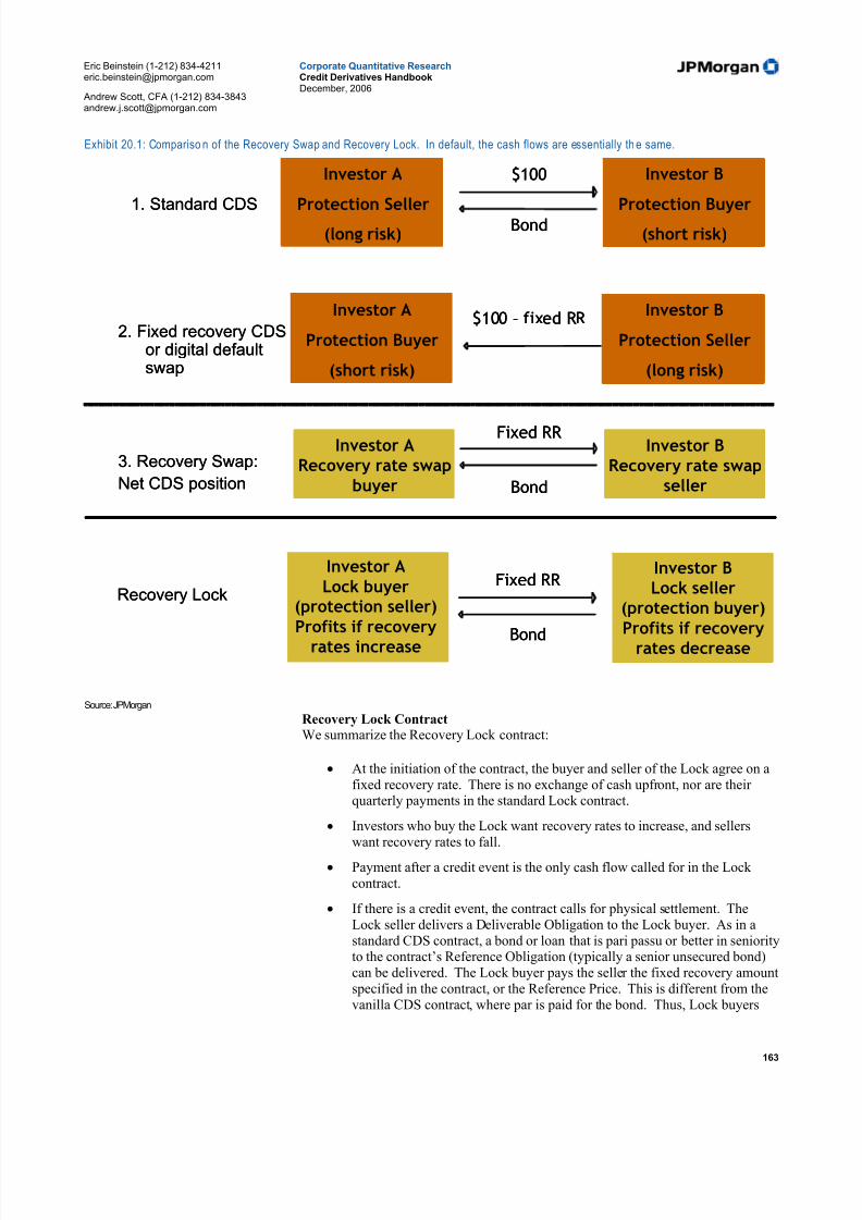
5/10/2018 JPM Credit Derivatives - slidepdf.com
http://slidepdf.com/reader/full/jpm-credit-derivatives-559e0102dc371 163/180
Eric Beinstein (1-212) [email protected]
Andrew Scott, CFA (1-212) [email protected]
Corporate Quantitative ResearchCredit Derivatives HandbookDecember, 2006
163
Exhibit 20.1: Compariso n of the Recovery Swap and Recovery Lock. In default, the cash flows are essentially th e same.
Investor A
Protection Seller(long risk)
1. Standard CDS
2. Fixed recovery CDSor digital defaultswap
3. Recovery Swap:
Net CDS position
Investor A
Protection Buyer
(short risk)
Bond
Investor B
Protection Buyer(short risk)
Investor B
Protection Seller
(long risk)
$100 – fixed RR
$100
Investor A
Recovery rate swap
buyer
Investor B
Recovery rate swap
seller
Fixed RR
Bond
Recovery Lock
Investor A
Lock buyer
(protection seller)
Profits if recoveryrates increase
Investor B
Lock seller
(protection buyer)
Profits if recoveryrates decrease
Fixed RR
Bond
Investor A
Protection Seller(long risk)
1. Standard CDS
2. Fixed recovery CDSor digital defaultswap
3. Recovery Swap:
Net CDS position
Investor A
Protection Buyer
(short risk)
Bond
Investor B
Protection Buyer(short risk)
Investor B
Protection Seller
(long risk)
$100 – fixed RR
$100
Investor A
Recovery rate swap
buyer
Investor B
Recovery rate swap
seller
Fixed RR
Bond
Recovery Lock
Investor A
Lock buyer
(protection seller)
Profits if recoveryrates increase
Investor B
Lock seller
(protection buyer)
Profits if recoveryrates decrease
Fixed RR
Bond
Source: JPMorgan
Recovery Lock Contract
We summarize the Recovery Lock contract:
• At the initiation of the contract, the buyer and seller of the Lock agree on afixed recovery rate. There is no exchange of cash upfront, nor are their quarterly payments in the standard Lock contract.
• Investors who buy the Lock want recovery rates to increase, and sellers
want recovery rates to fall.• Payment after a credit event is the only cash flow called for in the Lock
contract.
• If there is a credit event, the contract calls for physical settlement. TheLock seller delivers a Deliverable Obligation to the Lock buyer. As in astandard CDS contract, a bond or loan that is pari passu or better in seniorityto the contract’s Reference Obligation (typically a senior unsecured bond)can be delivered. The Lock buyer pays the seller the fixed recovery amountspecified in the contract, or the Reference Price. This is different from thevanilla CDS contract, where par is paid for the bond. Thus, Lock buyers
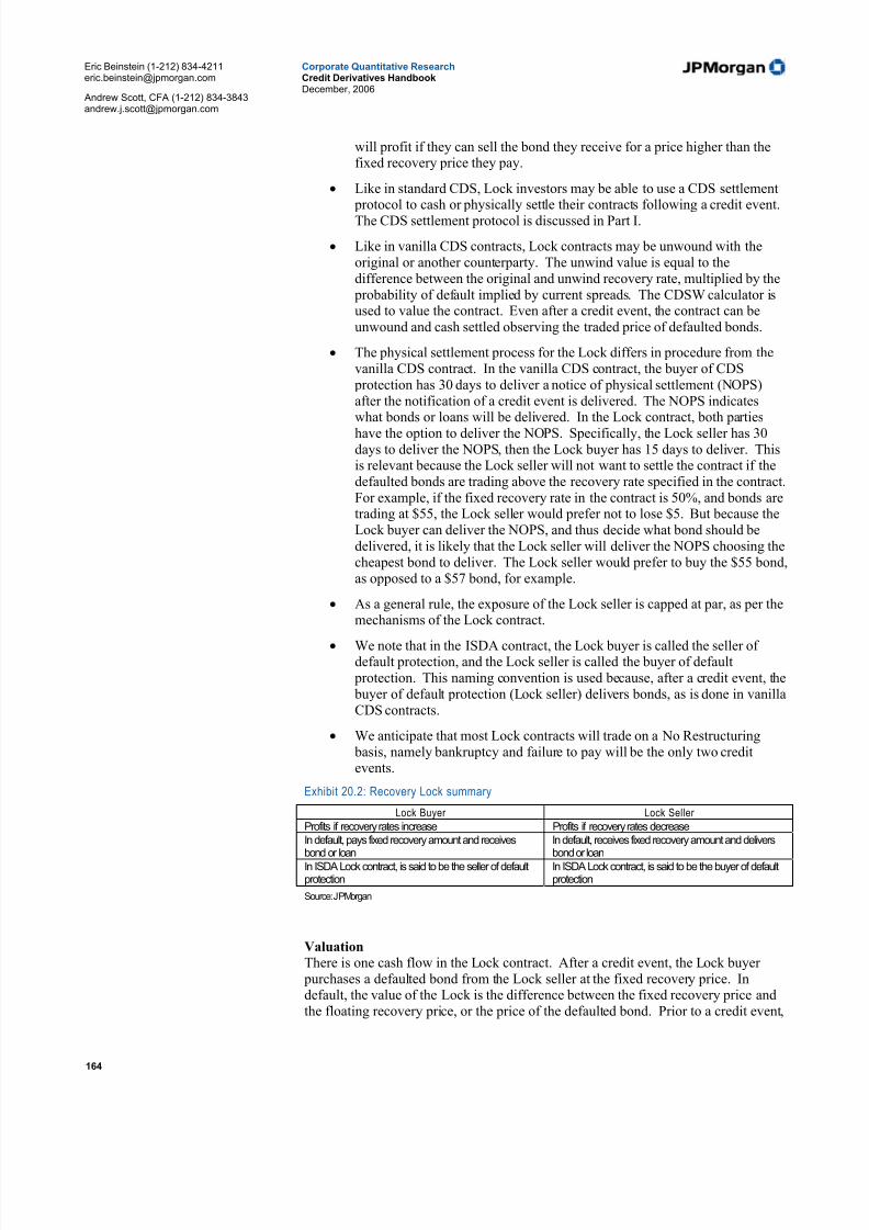
5/10/2018 JPM Credit Derivatives - slidepdf.com
http://slidepdf.com/reader/full/jpm-credit-derivatives-559e0102dc371 164/180
Eric Beinstein (1-212) [email protected]
Andrew Scott, CFA (1-212) [email protected]
Corporate Quantitative ResearchCredit Derivatives HandbookDecember, 2006
164
will profit if they can sell the bond they receive for a price higher than thefixed recovery price they pay.
• Like in standard CDS, Lock investors may be able to use a CDS settlement protocol to cash or physically settle their contracts following a credit event.The CDS settlement protocol is discussed in Part I.
• Like in vanilla CDS contracts, Lock contracts may be unwound with theoriginal or another counterparty. The unwind value is equal to thedifference between the original and unwind recovery rate, multiplied by the
probability of default implied by current spreads. The CDSW calculator isused to value the contract. Even after a credit event, the contract can beunwound and cash settled observing the traded price of defaulted bonds.
• The physical settlement process for the Lock differs in procedure from thevanilla CDS contract. In the vanilla CDS contract, the buyer of CDS
protection has 30 days to deliver a notice of physical settlement (NOPS)after the notification of a credit event is delivered. The NOPS indicateswhat bonds or loans will be delivered. In the Lock contract, both partieshave the option to deliver the NOPS. Specifically, the Lock seller has 30days to deliver the NOPS, then the Lock buyer has 15 days to deliver. Thisis relevant because the Lock seller will not want to settle the contract if thedefaulted bonds are trading above the recovery rate specified in the contract.For example, if the fixed recovery rate in the contract is 50%, and bonds aretrading at $55, the Lock seller would prefer not to lose $5. But because theLock buyer can deliver the NOPS, and thus decide what bond should bedelivered, it is likely that the Lock seller will deliver the NOPS choosing thecheapest bond to deliver. The Lock seller would prefer to buy the $55 bond,as opposed to a $57 bond, for example.
• As a general rule, the exposure of the Lock seller is capped at par, as per themechanisms of the Lock contract.
• We note that in the ISDA contract, the Lock buyer is called the seller of default protection, and the Lock seller is called the buyer of default
protection. This naming convention is used because, after a credit event, the buyer of default protection (Lock seller) delivers bonds, as is done in vanillaCDS contracts.
• We anticipate that most Lock contracts will trade on a No Restructuring basis, namely bankruptcy and failure to pay will be the only two creditevents.
Exhibit 20.2: Recovery Lock summary
Lock Buyer Lock Seller Profits if recovery rates increase Profits if recovery rates decreaseIn default, pays fixed recovery amount and receives
bond or loan
In default, receives fixed recovery amount and delivers
bond or loanIn ISDA Lock contract, is said to be the seller of defaultprotection
In ISDA Lock contract, is said to be the buyer of defaultprotection
Source: JPMorgan
Valuation
There is one cash flow in the Lock contract. After a credit event, the Lock buyer purchases a defaulted bond from the Lock seller at the fixed recovery price. Indefault, the value of the Lock is the difference between the fixed recovery price andthe floating recovery price, or the price of the defaulted bond. Prior to a credit event,

5/10/2018 JPM Credit Derivatives - slidepdf.com
http://slidepdf.com/reader/full/jpm-credit-derivatives-559e0102dc371 165/180
Eric Beinstein (1-212) [email protected]
Andrew Scott, CFA (1-212) [email protected]
Corporate Quantitative ResearchCredit Derivatives HandbookDecember, 2006
165
the value of the Lock is this difference multiplied by the probability of default, or the probability that the cash flow is realized.
The CDSW calculator on Bloomberg can be used to find the mark-to-market value,
but is used differently than in valuing standard CDS contracts. First, in the “DealInformation” section, three fields are adjusted compared to vanilla contracts:
Curve Recovery = False
Recovery Rate = 1 minus the absolute value of the difference between the fixedrate percentage and the current recovery rate
Deal Spread = 0bp, as there is not a running spread in the Lock contract
Second, the “Spreads” section of the calculator is used in the same manner as instandard CDS contracts. Current CDS spread levels are inputted, using either a flatspread or the entire CDS curve. Importantly, the current recovery rate level should
be entered into the “Recovery Rate” field. Based on the spreads and recovery rateinputted, the “Spreads” section calculates a default probability curve, or the
likelihood the credit will default over time. By multiplying the default probabilities by the recovery rate inputted in the Deal Information section, and summing this product through the maturity date of the contract, the calculator determines themarket value of the Lock.
Finally, the value of the Lock is displayed in the “Calculator” section in the “MarketValue” field.
Exhibit 20.3: Valuation o f our GMAC Recovery Lock example, where recovery rates changed by 4percentage points.
Source: Bloomberg, JPMorgan

5/10/2018 JPM Credit Derivatives - slidepdf.com
http://slidepdf.com/reader/full/jpm-credit-derivatives-559e0102dc371 166/180
Eric Beinstein (1-212) [email protected]
Andrew Scott, CFA (1-212) [email protected]
Corporate Quantitative ResearchCredit Derivatives HandbookDecember, 2006
166
Exhibit 20.4: Valuation of our Ford Motor Credit Recovery Lock example, where recovery rateschanged by 4 percentage points.
Source: Bloomberg, JPMorgan
As an example, assume we buy a Recovery Lock on GMAC at 68%, then unwind theLock at 72%, with CDS spreads trading at 320bp. The value of the Lock is $157K,given a $10 million notional. Note in Exhibit 20.4, the “Recovery Rate” entered inthe “Deal Information” section is .96, or 100% - |72% - 68%|, and the “Deal Spread”
= 0. Furthermore, assume we buy a Recovery Lock on Ford Motor Credit at 68%,then unwind the Lock at 72%, but CDS spreads are trading at 520bp. The value of the Lock is $219K, given a $10 million notional. The FMC market value is higher than GMAC because the probability that Ford defaults is higher than the probabilitythat GMAC defaults. Thus the Ford Recovery Lock unwind should be higher,
because the cash flow - which only occurs if there is a default - is more likely.
CDSW calculation intuition
The CDSW calculator values the future cash flows specified in the “DealInformation” section. From the point of view of the vanilla CDS protection seller (long risk), it essentially calculates the present value of the “Deal Spread” multiplied
by the probability the cash flows are realized, or one minus the probability of default.These probabilities are determined in the “Spreads” section, as the user inputs the
current CDS levels and recovery rate, implying the probability of default. In theLock, the “Deal Spread” is zero, thus the value of the vanilla CDS protection seller’scash flows is zero.
The CDSW calculator also values the future cash flows from the point of view of thevanilla CDS protection buyer (short risk). The protection buyer only receives cash if there is a credit event. In this case, the cash flow is equal to 1 minus the recoveryrate. Thus, to value the protection buyer’s cash flow, the CDSW calculator multiplies the cash payment following a credit event by the probability there is acredit event, then calculates the present value. Note, that if the recovery rate is100%, then in default, the protection buyer would purchase a bond for $100, deliver the bond to the seller of protection, and receive par for a net gain of zero. If the

5/10/2018 JPM Credit Derivatives - slidepdf.com
http://slidepdf.com/reader/full/jpm-credit-derivatives-559e0102dc371 167/180
Eric Beinstein (1-212) [email protected]
Andrew Scott, CFA (1-212) [email protected]
Corporate Quantitative ResearchCredit Derivatives HandbookDecember, 2006
167
recovery rate was 95%, then the protection buyer would purchase a bond at $95 andreceive par, netting $5.
In the Recovery Lock, the goal is to find the value of the difference between the
recovery rate specified in the contract and the current market recovery rate level.This cash flow is only realized if there is a credit event. Thus, we use the CDSWcalculator as described above, valuing this difference given the probability the cashflow will be realized. The probability the cash flow will be realized is calculated inthe “Spreads” section of the calculator, using the current CDS levels and recoveryrate. In the “Deal Information” section, setting the “Deal Spread” to zero and the“Recovery Rate” to 100% less the difference between Lock contract and currentmarket recovery rates, allows us to calculate the value based on current market
pricing.
Digital Default Swaps
A digital default swap (DDS) is a credit default swap where the payment to the buyer of protection following a credit event, normally 100% - recovery rate (the recoveryrate is determined after the credit event), is instead fixed at the trade’s inception. Allother aspects of the DDS contract are the same as the CDS contract. These structuresare also known as fixed recovery CDS because the payout is based on a fixedassumption about recovery following default rather than on market recovery rates.This instrument may be used to hedge specific exposures where the loss upon defaultis a known amount.
A special DDS is a zero recovery swap. In this contract, an investor pays or receivesa spread on a CDS that, in a credit event, will pay zero recovery. For example,assume a five year GMAC CDS quote of 405 / 410. An investor bullish on GMACcould sell protection (long credit risk) at 405bp. Alternatively, the investor could sellzero recovery protection at a spread above 405bp. The spread would be calculated
by dividing the CDS spread of 405bp by (1 – Recovery Rate). If the recovery rate in
the market is 60%, an investor could sell protection at 405 / 0.6 or 675bp. Theinvestor would thereby earn a significantly higher spread than the normal GMACCDS spread, but in a credit event, would suffer a greater loss. Namely, if the actual
price of GMAC bonds after a credit event were above $50, the investor would have been better off taking a long credit risk position in the regular CDS than in the zerorecovery CDS. If the actual recovery rate is below $50, the investor would have
been better off with the zero recovery CDS.

5/10/2018 JPM Credit Derivatives - slidepdf.com
http://slidepdf.com/reader/full/jpm-credit-derivatives-559e0102dc371 168/180
Eric Beinstein (1-212) [email protected]
Andrew Scott, CFA (1-212) [email protected]
Corporate Quantitative ResearchCredit Derivatives HandbookDecember, 2006
168
21. Other credit default swap products
Credit linked notes
Credit linked notes may be created for investors who are not able to invest in swaps.These products are typically created if an investor wanted a $100 million or larger
position to a particular credit, for example.
The economics of the credit default swap can be captured in a funded security or anote. A credit linked note is a synthetic security, typically issued by a special
purpose vehicle that trades like a bond issued by the reference entity but with theeconomics of the credit default swap. For this security, the buyer of protection sellsthe note. As in the credit default swap, the protection buyer is still “going shortrisk.” The buyer of protection (note seller) will pay periodic payments and profit if the reference entity defaults. Unlike the swap, the buyer of protection in a credit-linked note will receive money at the time of transaction from the sale of the note,
and will return this money at the contract’s maturity if no credit event occurs.
Conversely, the seller of protection purchases the note and is “long risk.” As with acredit default swap, the note purchaser (protection seller) receives periodic payments.Unlike the swap transaction, the protection seller must pay for the note at the time of the transaction and will collect this money at the contract’s maturity if no credit eventoccurs. Thus, the cash flows and risks of buying and selling credit-linked notes aresimilar to buying and selling bonds.
Recall that, in a credit default swap, if a reference entity has a credit event, the buyer of protection (short risk) delivers defaulted bonds or loans to the seller of protection(long risk), then receives the notional value of the credit default swap contract. Inother words, the buyer of protection receives par minus the recovery value of thedefaulted bond. When a reference entity of a credit linked note defaults, theeconomics are identical. In the case of default, the buyer of protection (short risk), or the investor who sold the note, delivers bonds and/or loans of the reference entity andkeeps the cash she received at the trade’s inception.
Exhibit 21.1: Credit-Linked Notes are a synthetic security that trades like a bond issued by theReference Entity, but with the economics of a credit default swap.
Source: JPMorgan.

5/10/2018 JPM Credit Derivatives - slidepdf.com
http://slidepdf.com/reader/full/jpm-credit-derivatives-559e0102dc371 169/180
Eric Beinstein (1-212) [email protected]
Andrew Scott, CFA (1-212) [email protected]
Corporate Quantitative ResearchCredit Derivatives HandbookDecember, 2006
169
Constant maturity credit default swaps (CMCDS)34 andcredit spread swaps (CSS)
Constant maturity credit default swaps are CDS contracts where the spread is reset
periodically, for example every six months, based on changes in the market spreadfor a benchmark CDS tenor. The benchmark CDS can be a single name or an index product. The buyer of protection (short risk) pays a fraction (called the participationrate, a rate negotiated at the initiation of the contract that remains constant) of thethen current credit default swap spread of the relevant maturity (called the referencerate). For example, the buyer of protection could pay 70% of the current five-year credit default swap spread on Company X, which is 100bp initially, but expected toincrease over time. If the five-year CDS spread on Company X six months later is125bp, the buyer of the constant maturity credit default swap would now pay 70% *125bp. This continues for the duration of the contract. If there is a credit eventduring the life of the contract, the contract terminates with a settlement procedureidentical to the credit default swap procedure, namely, the buyer of protection (shortrisk) delivers the notional amount of defaulted bonds to the seller of protection (longrisk), who then pays the notional amount to the buyer.
The buyer of protection in this example is taking the view that the spread on thecredit will increase by less than the spread implied by existing forward rates. At the
beginning of the contract, she is paying less for protection than if she had enteredinto a standard CDS contract. If the spread on the credit remains low, then she willcontinue to pay a low rate at each fixing, while if market spreads increasesignificantly, she will be obliged to pay much higher rates in the future. The initial
participation rate reflects this risk - it will generally be a lower number for steepcredit curves (i.e. perhaps 60%) and a higher number for flatter curves (i.e. 80%).
In a credit spread swap (CSS), an investor buys or sells protection using a CMCDScontract and enters into an offsetting default risk position using standard CDS. Thisstructure allows investors to take curve and directional spread exposure to a reference
entity without default risk.
Exhibit 21.2: Cons tant Maturit y CDS (CMCDS)
Source: JPMorgan.
34 For more information on CMCDS, refer to “Introduction to constant maturity CDS and CDOs” by JacobDue and Rishad Hluwalia published October 21, 2004.

5/10/2018 JPM Credit Derivatives - slidepdf.com
http://slidepdf.com/reader/full/jpm-credit-derivatives-559e0102dc371 170/180
Eric Beinstein (1-212) [email protected]
Andrew Scott, CFA (1-212) [email protected]
Corporate Quantitative ResearchCredit Derivatives HandbookDecember, 2006
170
First-to-default baskets35
In a first-to-default (FTD) basket, an investor chooses a basket of credits, typicallyfive names, instead of taking exposure to an individual credit default swap. If thereare no credit events, the basket pays a fixed coupon throughout the life of the trade.Upon a credit event in one of the basket names, the swap terminates, and the
protection buyer delivers the notional amount of the FTD basket in bonds or loans of the defaulted entity to the protection seller. The protection seller then pays the buyer the notional amount of the trade in cash. It is as if the protection seller (long risk)had written a contract on only the defaulted name.
A first-to-default basket is a leveraged position in a basket of credit default swaps. Itis a leveraged position because an investor is exposed to the risk of default on theentire basket rather than on a single name. However, the investor’s loss is limited tothe notional value of the trade. Because the basket has a higher probability of defaultthan an individual credit, the seller of protection receives a spread greater than thewidest individual spread in the basket. Typically, the basket pays a spread of 60-80% of the sum of the spreads in the basket. For example, Exhibit 21.4 is an
insurance company FTD basket that pays the seller of protection (long risk) 505 bp,which is 71% of the aggregate spread. The value drivers in this product are thenumber of basket components (the greater the number of names, the greater thelikelihood of one name defaulting, the greater the premium paid), absolute spreadlevels (clustered spreads provide the greatest value), and correlation (or similarity of assumed default probability between credits, the less similar the correlation, thehigher the default risk, therefore the greater the premium paid).
Exhibit 21.3: First-to-default baskets
Source: JPMorgan
Exhibit 21.4: Sample High Yield FTD Basket
Reference Credits 5yr Bid S&P Industry
ACE LIMITED 125 Insurance
AIG CORP 27 Insurance
AON CORP 245 InsuranceMARSH & MCLENNAN 250 Insurance
HARTFORD FIN. GROUP 62 Insurance
AGGREGATE SPREAD 709 Bps
5YR First to Default Spread over LIBOR 505 Bps
5YR First to Default % of Aggregate Spread 71% Source: JPMorgan
35 For more information on First to default baskets, refer to “First-to-Default Baskets: A Primer,” byRishad Ahluwalia, published October 24, 2003.

5/10/2018 JPM Credit Derivatives - slidepdf.com
http://slidepdf.com/reader/full/jpm-credit-derivatives-559e0102dc371 171/180
Eric Beinstein (1-212) [email protected]
Andrew Scott, CFA (1-212) [email protected]
Corporate Quantitative ResearchCredit Derivatives HandbookDecember, 2006
171
Conclusion
The use of credit derivatives has grown exponentially since the beginning of thedecade. Transaction volumes have picked up from the occasional tens of millions of dollars to regular weekly volumes measured in many billions of dollars. The end-user
base is broadening rapidly to include a wide range of banks, broker-dealers,institutional investors, asset managers, corporations, hedge funds, insurers, andreinsurers. Growth in participation and market volume are likely to continue basedon the investment opportunities created by the products. While we do not expect thecredit derivatives market to reach the 50:1 derivative to cash ratio in the interest ratemarket anytime soon, we do expect growth to continue.
Interest rate market$ trillion notional
Credit market$ trillion notional
$213.00
$4.30
Derivatives Treasury Bonds
Derivatives$17.1
Corporate
Bonds $4.15High grade $3.2High yield $.95
$20.21
$14.62
Derivatives Cash Bonds
Interest rate market$ trillion notional
Credit market$ trillion notional
$213.00
$4.30
Derivatives Treasury Bonds
Derivatives$17.1
Corporate
Bonds $4.15High grade $3.2High yield $.95
$20.21
$14.62
Derivatives Cash Bonds
Source: British Bankers’ Association, Bank for International Settlements, Bureau of the Public Debt, and JPMorgan Estimates.

5/10/2018 JPM Credit Derivatives - slidepdf.com
http://slidepdf.com/reader/full/jpm-credit-derivatives-559e0102dc371 172/180
Eric Beinstein (1-212) [email protected]
Andrew Scott, CFA (1-212) [email protected]
Corporate Quantitative ResearchCredit Derivatives HandbookDecember, 2006
172
Appendix I: JPMorgan CDSW ExampleCalculations Model
(for illustration of the general concepts only)
Notional value 10,000,000
Initial contract spread 5.00%
Current at market Spd 4.00%
Recovery assumption 40%
Clean spread 6.667% Add it ional Check o f calcu lat ion
(probability of default)
Col 1 Col 2 Col 3 Col 4 Col 5 Col 6 Col 7 Col 8 Col 9 Col 10 Col 11
Premium
Cash Flow Paid on PV o f Value of Value o f
Earned on of fset t ing Net Swap Discoun t Prob o f Survival Expected Current Coupon loss if default
Period CDS CDS Premium Curve Factor Default Probability Cash f lows Flows
0.25 $125,000 $100,000 $25,000 2.000% 0.99502 0.0160 0.9840 $24,477 $97,910 $95,553
0.50 $125,000 $100,000 $25,000 2.000% 0.99007 0.0157 0.9682 $23,966 $95,864 $93,556
0.75 $125,000 $100,000 $25,000 2.000% 0.98515 0.0155 0.9527 $23,465 $93,860 $91,601
1.00 $125,000 $100,000 $25,000 2.000% 0.98025 0.0152 0.9375 $22,975 $91,898 $89,686
1.25 $125,000 $100,000 $25,000 2.000% 0.97537 0.0150 0.9225 $22,494 $89,977 $87,812
1.50 $125,000 $100,000 $25,000 2.000% 0.97052 0.0148 0.9077 $22,024 $88,097 $85,976
1.75 $125,000 $100,000 $25,000 2.000% 0.96569 0.0145 0.8932 $21,564 $86,256 $84,179
2.00 $125,000 $100,000 $25,000 2.000% 0.96089 0.0143 0.8789 $21,113 $84,453 $82,420
2.25 $125,000 $100,000 $25,000 2.000% 0.95610 0.0141 0.8648 $20,672 $82,688 $80,697
2.50 $125,000 $100,000 $25,000 2.000% 0.95135 0.0138 0.8510 $20,240 $80,959 $79,011
2.75 $125,000 $100,000 $25,000 2.000% 0.94661 0.0136 0.8374 $19,817 $79,267 $77,359
3.00 $125,000 $100,000 $25,000 2.000% 0.94191 0.0134 0.8240 $19,403 $77,611 $75,743
3.25 $125,000 $100,000 $25,000 2.000% 0.93722 0.0132 0.8108 $18,997 $75,988 $74,159
3.50 $125,000 $100,000 $25,000 2.000% 0.93256 0.0130 0.7978 $18,600 $74,400 $72,609
3.75 $125,000 $100,000 $25,000 2.000% 0.92792 0.0128 0.7850 $18,211 $72,845 $71,092
4.00 $125,000 $100,000 $25,000 2.000% 0.92330 0.0126 0.7725 $17,831 $71,323 $69,606
4.25 $125,000 $100,000 $25,000 2.000% 0.91871 0.0124 0.7601 $17,458 $69,832 $68,151
4.50 $125,000 $100,000 $25,000 2.000% 0.91414 0.0122 0.7479 $17,093 $68,373 $66,727
4.75 $125,000 $100,000 $25,000 2.000% 0.90959 0.0120 0.7360 $16,736 $66,943 $65,332
5.00 $125,000 $100,000 $25,000 2.000% 0.90506 0.0118 0.7242 $16,386 $65,544 $63,967
Mark to market of CDS unwind $403,522 $1,614,089 $1,575,237
Dif feren ce o f su ms: -$38,851
Ente r the cur rent mark e t sp read
Notional Value *Orig inal Contrac t
Spread / 4 ( f o r
quar te r l y
p a y men t )
Notional Value *
Current
M a r k e t
Spread / 4
( fo r qua r te r l y
p a y men t s
Dif ferencebe tween
Co lumn 2 and
Column 3. This
rep resents thecash f low which
i s be ing va lued -
I .e. the v alue of
a CDS unwind is
the d i s counted
value of this
cash f low
s t ream
Ente r the assumed Recovery Ra te
Equa l to cur rent mark e t sp read / (1 - Re covery Ra te ) . I t i s the annua l de fau l tprobabi l i ty . This is an approx imat ion which is correct i f one is do ing the ca lculat ions
assum ing continuous poss ib i l i ty of default. I t is s l ightly of f when assu ming default is
on ly poss ib le on the quar t e r l y paym ent da tes , as we do be low.
Ente r no t iona l pos i t i on amount
Ente r the o r ig ina l cont ract coupon
Probabi l i ty of no default.Ca l cu la ted as 1 / (1+
C lean Spread) ̂ t ime in
yea rs . The concept is
tha t the c lean sp read i s
the annua l de fau l t
probabi l i ty . The
probabi l i ty of not hav ing
de fau l ted a f te r two
years ( f o r exam p le ) is
the proba bi l i ty of no
de fau l t in yea r one
mul t ip l ied by the
probabi l i ty of no default
in yea r two .
1 M inus Co lumn 8
Column 4 XColumn 6 X
Column 8.
The cash f lows
expected X thed i s count f ac to r
fo r t ime X the
probabi l i ty of
rece iv ing the
cash f lows.
When a CDS i s a t pa r i tmea n s t h a t t h e e x pe c t e
va lue o f the cash f lows t
rece ived (wi th no de fau
equa l to the expected v
o f the recovery va lue to
rece ived ( in case o f
default). These ca lculata re shown in co lumns 10
and 11 below. The co lum
gener al ly wi l l be a l i tt le
because the C lean Sprea
which is ca lculated as
Current Marke t Spread
Recovery ) i s no t qu i te r
because o f cont inuous v
d i s cre te com pound ing, a
d i s cussed .
Source: JPMorgan

5/10/2018 JPM Credit Derivatives - slidepdf.com
http://slidepdf.com/reader/full/jpm-credit-derivatives-559e0102dc371 173/180
Eric Beinstein (1-212) [email protected]
Andrew Scott, CFA (1-212) [email protected]
Corporate Quantitative ResearchCredit Derivatives HandbookDecember, 2006
173
Appendix II: How to get CDX and iTraxxdata
Historical data on the CDX and iTraxx indices are available on the DataQuery tool(http://dataquery.jpmorgan.com/index.jsp) on MorganMarkets. Using this tool,
prices, spreads, basis to theoretical value and duration for current and predecessor indices can be retrieved. The path to retrieve the CDX data, for example, is:
Credit → Credit Default Swaps → Indices → North America
iTraxx data for Europe and Asia, and EM CDX data is available through a similar path.
Source: JPMorgan

5/10/2018 JPM Credit Derivatives - slidepdf.com
http://slidepdf.com/reader/full/jpm-credit-derivatives-559e0102dc371 174/180
Eric Beinstein (1-212) [email protected]
Andrew Scott, CFA (1-212) [email protected]
Corporate Quantitative ResearchCredit Derivatives HandbookDecember, 2006
174
Companies Recommended in This Report (all prices in this report as of market close on 27 November 2006, unless
otherwise indicated)
Alltel (AT/$55.78/Overweight), American Axle & Manufacturing Holdings, Inc. (AXL/$18.06/Neutral), General Motors(GM/$30.36/Neutral), Lear Corporation (LEA/$30.67/Neutral), Windstream Communications (WIN/$13.62/Neutral)
Analyst Certification:
The research analyst(s) denoted by an “AC” on the cover of this report certifies (or, where multiple research analysts are primarilyresponsible for this report, the research analyst denoted by an “AC” on the cover or within the document individually certifies, withrespect to each security or issuer that the research analyst covers in this research) that: (1) all of the views expressed in this reportaccurately reflect his or her personal views about any and all of the subject securities or issuers; and (2) no part of any of the researchanalyst’s compensation was, is, or will be directly or indirectly related to the specific recommendations or views expressed by theresearch analyst(s) in this report.
Conflict of Interest
This research contains the views, opinions and recommendations of JP Morgan credit research analysts. Research analysts
routinely consult with JPMorgan trading desk personnel in formulating views, opinions and recommendations in preparing
research. Trading desks may trade or have traded as principal on the basis of the research analyst(s) views and report(s).
Therefore, this research may not be independent from the proprietary interests of JPMorgan trading desks which may conflict
with your interests. In addition, research analysts receive compensation based, in part, on the quality and accuracy of their
analysis, client feedback, trading desk and firm revenues and competitive factors. As a general matter, JPMorgan and/or its
affiliates normally make a market and trade as principal in fixed income securities discussed in research reports.
Important Disclosures
• Lead or Co-manager: JPMSI or its affiliates acted as lead or co-manager in a public offering of equity and/or debt
securities for American Axle & Manufacturing Holdings, Inc., Dana Corp., General Motors, Lear Corporation
within the past 12 months.
• Beneficial Ownership (1% or more): JPMSI or its affiliates beneficially own 1% or more of a class of common
equity securities of American Axle & Manufacturing Holdings, Inc., General Motors, Lear Corporation.
• Client of the Firm: Alltel is or was in the past 12 months a client of JPMSI; during the past 12 months, JPMSI
provided to the company investment banking services, non-investment banking securities-related service and
non-securities-related services. American Axle & Manufacturing Holdings, Inc. is or was in the past 12 months a
client of JPMSI; during the past 12 months, JPMSI provided to the company investment banking services andnon-securities-related services. Dana Corp. is or was in the past 12 months a client of JPMSI; during the past 12
months, JPMSI provided to the company non-investment banking securities-related service and non-securities-
related services. General Motors is or was in the past 12 months a client of JPMSI; during the past 12 months,
JPMSI provided to the company investment banking services, non-investment banking securities-related service
and non-securities-related services. General Motors Acceptance Corporation is or was in the past 12 months a
client of JPMSI; during the past 12 months, JPMSI provided to the company investment banking services, non-
investment banking securities-related service and non-securities-related services. Lear Corporation is or was in
the past 12 months a client of JPMSI; during the past 12 months, JPMSI provided to the company investment
banking services, non-investment banking securities-related service and non-securities-related services.
Windstream Communications is or was in the past 12 months a client of JPMSI; during the past 12 months,
JPMSI provided to the company investment banking services.
• Investment Banking (past 12 months): JPMSI or its affiliates received in the past 12 months compensation for
investment banking services from Alltel, American Axle & Manufacturing Holdings, Inc., General Motors,
General Motors Acceptance Corporation, Lear Corporation, Windstream Communications.
• Investment Banking (next 3 months): JPMSI or its affiliates expect to receive, or intend to seek, compensation for
investment banking services in the next three months from Alltel, American Axle & Manufacturing Holdings,
Inc., Dana Corp., General Motors, General Motors Acceptance Corporation, Lear Corporation, Windstream
Communications.
• Non-Investment Banking Compensation: JPMSI has received compensation in the past 12 months for products or
services other than investment banking from Alltel, Dana Corp., General Motors, General Motors Acceptance
Corporation, Lear Corporation. An affiliate of JPMSI has received compensation in the past 12 months for
products or services other than investment banking from Alltel, American Axle & Manufacturing Holdings,
Inc., Dana Corp., General Motors, General Motors Acceptance Corporation, Lear Corporation.

5/10/2018 JPM Credit Derivatives - slidepdf.com
http://slidepdf.com/reader/full/jpm-credit-derivatives-559e0102dc371 175/180
Eric Beinstein (1-212) [email protected]
Andrew Scott, CFA (1-212) [email protected]
Corporate Quantitative ResearchCredit Derivatives HandbookDecember, 2006
175
• J.P. Morgan Securities Inc and/or its affiliates is acting as a financial advisor to Alltel Corporation ("AT") in
connection with its proposed spinoff/sale of its Wireline business segment ("Alltel Wireline") to VALOR
Communications Group, Inc. ("VCG") in a Reverse Morris Trust transaction announced on December 9, 2005.
The proposed transaction is subject to regulatory and VALOR shareholder approvals. This research report and
the information herein is not intended to provide voting advice, serve as an endorsement of the proposedtransaction or result in procurement, withholding or revocation of a proxy or any other action by a security
holder.
• JP Morgan and/or its affiliates is advising General Motors Corp. on the sale of a 17.4% stake in Japan's Suzuki
Motor Corp.
• JP Morgan and/or its affiliates is advising General Motors Corp. on the sale of a 17.4% stake in Japan's Suzuki
Motor Corp.
• J.P. Morgan Securities Inc and/or its affiliates is acting as a financial advisor to Alltel Corporation ("AT") in
connection with its proposed spinoff/sale of its Wireline business segment ("Alltel Wireline") to VALOR
Communications Group, Inc. ("VCG") in a Reverse Morris Trust transaction announced on December 9, 2005.
The proposed transaction is subject to regulatory and VALOR shareholder approvals. This research report and
the information herein is not intended to provide voting advice, serve as an endorsement of the proposed
transaction or result in procurement, withholding or revocation of a proxy or any other action by a security
holder.
Explanation of Credit Research Ratings:
Ratings System: JPMorgan uses the following sector/issuer portfolio weightings: Overweight (over the next three months, therecommended risk position is expected to outperform the relevant index, sector, or benchmark), Neutral (over the next three months, therecommended risk position is expected to perform in line with the relevant index, sector, or benchmark), and Underweight (over the nextthree months, the recommended risk position is expected to underperform the relevant index, sector, or benchmark). JPMorgan’sEmerging Market research uses a rating of Marketweight, which is equivalent to a Neutral rating.
Valuation & Methodology: In JPMorgan’s credit research, we assign a rating to each issuer (Overweight, Underweight or Neutral) based on our credit view of the issuer and the relative value of its securities, taking into account the ratings assigned to the issuer by creditrating agencies and the market prices for the issuer’s securities. Our credit view of an issuer is based upon our opinion as to whether theissuer will be able service its debt obligations when they become due and payable. We assess this by analyzing, among other things, theissuer’s credit position using standard credit ratios such as cash flow to debt and fixed charge coverage (including and excluding capitalinvestment). We also analyze the issuer’s ability to generate cash flow by reviewing standard operational measures for comparable
companies in the sector, such as revenue and earnings growth rates, margins, and the composition of the issuer’s balance sheet relative tothe operational leverage in its business.
0
15
30
45
60
75
90
105
120
Price($)
Nov
03
Feb
04
May
04
Aug
04
Nov
04
Feb
05
May
05
Aug
05
Nov
05
Feb
06
May
06
Aug
06
Nov
06
Alltel (AT) Price Chart
N OW OW $79 OW $86 OW $73
Source: Reuters and JPMorgan; price data adjusted for stock splits and dividends.
This chart shows JPMorgan's continuing coverage of this stock; the current analyst may or may not have covered it over
the entire period. As of Aug. 30, 2002, the firm discontinued price targets in all markets where they were used. They
were reinstated at JPMSI as of May 19th, 2003, for Focus List (FL) and selected Latin stocks. For non-JPMSI covered
stocks, price targets are required for regional FL stocks and may be set for other stocks at analysts' discretion.
JPMorgan ratings: OW = Overweight, N = Neutral, UW = Underweight.
Date Rating Share Price($)
Price Targe($)
13-Jan-04 N 48.97 -
23-Apr-04 OW 50.81 -

5/10/2018 JPM Credit Derivatives - slidepdf.com
http://slidepdf.com/reader/full/jpm-credit-derivatives-559e0102dc371 176/180
Eric Beinstein (1-212) [email protected]
Andrew Scott, CFA (1-212) [email protected]
Corporate Quantitative ResearchCredit Derivatives HandbookDecember, 2006
176
0
10
20
30
40
50
60
70
Price($)
Nov
03
Feb
04
May
04
Aug
04
Nov
04
Feb
05
May
05
Aug
05
Nov
05
Feb
06
May
06
Aug
06
Nov
06
American Axle & Manufacturing Holdings, Inc. (AXL) Price Chart
N
Source: Reuters and JPMorgan; price data adjusted for stock splits and dividends.
Initiated coverage Sep 28, 2004. This chart shows JPMorgan's continuing coverage of this stock; the current analyst may
or may not have covered it over the entire period. As of Aug. 30, 2002, the firm discontinued price targets in all
markets where they were used. They were reinstated at JPMSI as of May 19th, 2003, for Focus List (FL) and selected Latin
stocks. For non-JPMSI covered stocks, price targets are required for regional FL stocks and may be set for other stocks
at analysts' discretion.
JPMorgan ratings: OW = Overweight, N = Neutral, UW = Underweight.
Date Rating Share Price($)
Price Targe($)
28-Sep-04 N 28.45 -
0
15
30
45
60
75
90
Price($)
Nov03
Feb04
May04
Aug04
Nov04
Feb05
May05
Aug05
Nov05
Feb06
May06
Aug06
Nov06
General Motors (GM) Price Chart
N OW N
Source: Reuters and JPMorgan; price data adjusted for stock splits and dividends.
Break in coverage Apr 16, 2003 - Jun 12, 2003. This chart shows JPMorgan's continuing coverage of this stock; the
current analyst may or may not have covered it over the entire period. As of Aug. 30, 2002, the firm discontinued price
targets in all markets where they were used. They were reinstated at JPMSI as of May 19th, 2003, for Focus List (FL) and
selected Latin stocks. For non-JPMSI covered stocks, price targets are required for regional FL stocks and may be set
for other stocks at analysts' discretion.
JPMorgan ratings: OW = Overweight, N = Neutral, UW = Underweight.
Date Rating Share Price($)
Price Targe($)
10-Feb-04 N 49.11 -
05-May-05 OW 32.80 -
17-Aug-06 N 30.99 -

5/10/2018 JPM Credit Derivatives - slidepdf.com
http://slidepdf.com/reader/full/jpm-credit-derivatives-559e0102dc371 177/180
Eric Beinstein (1-212) [email protected]
Andrew Scott, CFA (1-212) [email protected]
Corporate Quantitative ResearchCredit Derivatives HandbookDecember, 2006
177
0
20
40
60
80
100
120
Price($)
Nov
03
Feb
04
May
04
Aug
04
Nov
04
Feb
05
May
05
Aug
05
Nov
05
Feb
06
May
06
Aug
06
Nov
06
Lear Corporation (LEA) Price Chart
N
Source: Reuters and JPMorgan; price data adjusted for stock splits and dividends.
This chart shows JPMorgan's continuing coverage of this stock; the current analyst may or may not have covered it over
the entire period. As of Aug. 30, 2002, the firm discontinued price targets in all markets where they were used. They
were reinstated at JPMSI as of May 19th, 2003, for Focus List (FL) and selected Latin stocks. For non-JPMSI covered
stocks, price targets are required for regional FL stocks and may be set for other stocks at analysts' discretion.
JPMorgan ratings: OW = Overweight, N = Neutral, UW = Underweight.
Date Rating Share Price($)
Price Targe($)
02-Mar-05 N 52.76 -
02
4
6
8
10
12
14
16
18
20
22
24
26
Price($)
Feb05
May05
Aug05
Nov05
Feb06
May06
Aug06
Nov06
Windstream Communications (WIN) Price Chart
N
Source: Reuters and JPMorgan; price data adjusted for stock splits and dividends.
Initiated coverage Apr 20, 2005. This chart shows JPMorgan's continuing coverage of this stock; the current analyst may
or may not have covered it over the entire period. As of Aug. 30, 2002, the firm discontinued price targets in all
markets where they were used. They were reinstated at JPMSI as of May 19th, 2003, for Focus List (FL) and selected Latin
stocks. For non-JPMSI covered stocks, price targets are required for regional FL stocks and may be set for other stocks
at analysts' discretion.
JPMorgan ratings: OW = Overweight, N = Neutral, UW = Underweight.
Date Rating Share Price($)
Price Targe($)
20-Apr-05 N 14.30 -
Explanation of Equity Research Ratings and Analyst(s) Coverage Universe:
JPMorgan uses the following rating system: Overweight [Over the next six to twelve months, we expect this stock will outperform theaverage total return of the stocks in the analyst’s (or the analyst’s team’s) coverage universe.] Neutral [Over the next six to twelve
months, we expect this stock will perform in line with the average total return of the stocks in the analyst’s (or the analyst’s team’s)coverage universe.] Underweight [Over the next six to twelve months, we expect this stock will underperform the average total return of the stocks in the analyst’s (or the analyst’s team’s) coverage universe.] The analyst or analyst’s team’s coverage universe is the sector and/or country shown on the cover of each publication. See below for the specific stocks in the certifying analyst(s) coverage universe.

5/10/2018 JPM Credit Derivatives - slidepdf.com
http://slidepdf.com/reader/full/jpm-credit-derivatives-559e0102dc371 178/180
Eric Beinstein (1-212) [email protected]
Andrew Scott, CFA (1-212) [email protected]
Corporate Quantitative ResearchCredit Derivatives HandbookDecember, 2006
178
JPMorgan Equity Research Ratings Distribution, as of September 29, 2006
Overweight
(buy)Neutral
(hold)Underweight
(sell)
JPM Global Equity Research Coverage 42% 41% 17%IB clients* 44% 46% 35%
JPMSI Equity Research Coverage 38% 48% 15%IB clients* 62% 55% 47%
*Percentage of investment banking clients in each rating category.For purposes only of NASD/NYSE ratings distribution rules, our Overweight rating falls into a buy rating category; our Neutral rating falls into a holdrating category; and our Underweight rating falls into a sell rating category.
Valuation and Risks: Please see the most recent JPMorgan research report for an analysis of valuation methodology and risks on anysecurities recommended herein. Research is available at http://www.morganmarkets.com , or you can contact the analyst named on thefront of this note or your JPMorgan representative.
Analysts’ Compensation: The research analysts responsible for the preparation of this report receive compensation based upon variousfactors, including the quality and accuracy of research, client feedback, competitive factors, and overall firm revenues, which includerevenues from, among other business units, Institutional Equities, Fixed Income, and Investment Banking.
Other Disclosures
Options related research: If the information contained herein regards options related research, such information is available only to persons whohave received the proper option risk disclosure documents. For a copy of the Option Clearing Corporation’s Characteristics and Risks of Standardized Options, please contact your JPMorgan Representative or visit the OCC’s website athttp://www.optionsclearing.com/publications/risks/riskstoc.pdf.
Legal Entities DisclosuresU.S.: JPMSI is a member of NYSE, NASD and SIPC. J.P. Morgan Futures Inc. is a member of the NFA. J.P. Morgan Chase Bank, N.A. is amember of FDIC and is authorized and regulated in the UK by the Financial Services Authority. U.K.: J.P. Morgan Securities Ltd. (JPMSL) is amember of the London Stock Exchange and is authorised and regulated by the Financial Services Authority. South Africa: J.P. Morgan EquitiesLimited is a member of the Johannesburg Securities Exchange and is regulated by the FSB. Hong Kong: J.P. Morgan Securities (Asia Pacific)Limited (CE number AAJ321) is regulated by the Hong Kong Monetary Authority and the Securities and Futures Commission in Hong Kong.Korea: J.P. Morgan Securities (Far East) Ltd, Seoul branch, is regulated by the Korea Financial Supervisory Service. Australia: J.P. MorganAustralia Limited (ABN 52 002 888 011/AFS Licence No: 238188, regulated by ASIC) and J.P. Morgan Securities Australia Limited (ABN 61003 245 234/AFS Licence No: 238066, a Market Participant with the ASX) (JPMSAL) are licensed securities dealers. Taiwan: J.P.MorganSecurities (Taiwan) Limited is a participant of the Taiwan Stock Exchange (company-type) and regulated by the Taiwan Securities and FuturesCommission. India: J.P. Morgan India Private Limited is a member of the National Stock Exchange of India Limited and The Stock Exchange,Mumbai and is regulated by the Securities and Exchange Board of India. Thailand: JPMorgan Securities (Thailand) Limited is a member of theStock Exchange of Thailand and is regulated by the Ministry of Finance and the Securities and Exchange Commission. Indonesia: PT J.P.Morgan Securities Indonesia is a member of the Jakarta Stock Exchange and Surabaya Stock Exchange and is regulated by the BAPEPAM.Philippines: This report is distributed in the Philippines by J.P. Morgan Securities Philippines, Inc. Brazil: Banco J.P. Morgan S.A. is regulated
by the Comissao de Valores Mobiliarios (CVM) and by the Central Bank of Brazil. Japan: This material is distributed in Japan by JPMorganSecurities Japan Co., Ltd., which is regulated by the Japan Financial Services Agency (FSA). Singapore: This material is issued and distributedin Singapore by J.P. Morgan Securities Singapore Private Limited (JPMSS) [mica (p) 069/09/2006 and Co. Reg. No.: 199405335R] which is amember of the Singapore Exchange Securities Trading Limited and is regulated by the Monetary Authority of Singapore (MAS) and/or JPMorganChase Bank, N.A., Singapore branch (JPMCB Singapore) which is regulated by the MAS. Malaysia: This material is issued and distributed inMalaysia by JPMorgan Securities (Malaysia) Sdn Bhd (18146-x) (formerly known as J.P. Morgan Malaysia Sdn Bhd) which is a ParticipatingOrganization of Bursa Malaysia Securities Bhd and is licensed as a dealer by the Securities Commission in Malaysia
Country and Region Specific Disclosures
U.K. and European Economic Area (EEA): Issued and approved for distribution in the U.K. and the EEA by JPMSL. Investment researchissued by JPMSL has been prepared in accordance with JPMSL’s Policies for Managing Conflicts of Interest in Connection with InvestmentResearch which can be found at http://www.jpmorgan.com/pdfdoc/research/ConflictManagementPolicy.pdf. This report has been issued in theU.K. only to persons of a kind described in Article 19 (5), 38, 47 and 49 of the Financial Services and Markets Act 2000 (Financial Promotion)Order 2001 (all such persons being referred to as "relevant persons"). This document must not be acted on or relied on by persons who are notrelevant persons. Any investment or investment activity to which this document relates is only available to relevant persons and will be engagedin only with relevant persons. In other EEA countries, the report has been issued to persons regarded as professional investors (or equivalent) intheir home jurisdiction Germany: This material is distributed in Germany by J.P. Morgan Securities Ltd. Frankfurt Branch and JPMorgan ChaseBank, N.A., Frankfurt Branch who are regulated by the Bundesanstalt für Finanzdienstleistungsaufsicht. Australia: This material is issued anddistributed by JPMSAL in Australia to “wholesale clients” only. JPMSAL does not issue or distribute this material to “retail clients.” Therecipient of this material must not distribute it to any third party or outside Australia without the prior written consent of JPMSAL. For the
purposes of this paragraph the terms “wholesale client” and “retail client” have the meanings given to them in section 761G of the CorporationsAct 2001. Hong Kong: The 1% ownership disclosure as of the previous month end satisfies the requirements under Paragraph 16.5(a) of theHong Kong Code of Conduct for persons licensed by or registered with the Securities and Futures Commission. (For research published within

5/10/2018 JPM Credit Derivatives - slidepdf.com
http://slidepdf.com/reader/full/jpm-credit-derivatives-559e0102dc371 179/180
Eric Beinstein (1-212) [email protected]
Andrew Scott, CFA (1-212) [email protected]
Corporate Quantitative ResearchCredit Derivatives HandbookDecember, 2006
179
the first ten days of the month, the disclosure may be based on the month end data from two months’ prior.) J.P. Morgan Broking (Hong Kong)Limited is the liquidity provider for derivative warrants issued by J.P. Morgan International Derivatives Ltd and listed on The Stock Exchange of Hong Kong Limited. An updated list can be found on HKEx website: http://www.hkex.com.hk/prod/dw/Lp.htm. Korea: This report may have
been edited or contributed to from time to time by affiliates of J.P. Morgan Securities (Far East) Ltd, Seoul branch. Singapore: JPMSI and/or itsaffiliates may have a holding in any of the securities discussed in this report; for securities where the holding is 1% or greater, the specific holding
is disclosed in the Legal Disclosures section above. India: For private circulation only not for sale. New Zealand: This material is issued anddistributed by JPMSAL in New Zealand only to persons whose principal business is the investment of money or who, in the course of and for the
purposes of their business, habitually invest money. JPMSAL does not issue or distribute this material to members of "the public" as determinedin accordance with section 3 of the Securities Act 1978. The recipient of this material must not distribute it to any third party or outside NewZealand without the prior written consent of JPMSAL.
General: Additional information is available upon request. Information has been obtained from sources believed to be reliable but JPMorganChase & Co. or its affiliates and/or subsidiaries (collectively JPMorgan) do not warrant its completeness or accuracy except with respect to anydisclosures relative to JPMSI and/or its affiliates and the analyst’s involvement with the issuer that is the subject of the research. All pricing is asof the close of market for the securities discussed, unless otherwise stated. Opinions and estimates constitute our judgment as of the date of thismaterial and are subject to change without notice. Past performance is not indicative of future results. This material is not intended as an offer or solicitation for the purchase or sale of any financial instrument. The opinions and recommendations herein do not take into account individualclient circumstances, objectives, or needs and are not intended as recommendations of particular securities, financial instruments or strategies to
particular clients. The recipient of this report must make its own independent decisions regarding any securities or financial instrumentsmentioned herein. JPMSI distributes in the U.S. research published by non-U.S. affiliates and accepts responsibility for its contents. Periodicupdates may be provided on companies/industries based on company specific developments or announcements, market conditions or any other
publicly available information. Clients should contact analysts and execute transactions through a JPMorgan subsidiary or affiliate in their home jurisdiction unless governing law permits otherwise.
Revised September 30, 2006.
Copyright 2006 JPMorgan Chase & Co. All rights reserved. This report or any portion hereof may not be reprinted, sold or
redistributed without the written consent of JPMorgan.

5/10/2018 JPM Credit Derivatives - slidepdf.com
http://slidepdf.com/reader/full/jpm-credit-derivatives-559e0102dc371 180/180