journal of technical analysis (jota). issue 14 (1982, august)

Market Technicians Association

JOURNAL Issue 14 August 1982

PWKET TECHNICIANS ASSOCIATION JOURML

Issue 14

August, 1982

Published by : Market Technicians Association 70 Pine Street

New York, New York 10005

Copyright 1982 by Market Technicians Association

-l-

intentionally blank

-2-

Market Technicians Association Journal

Editor :

Associate Editor :

Anthony W. Tabell Delafield , Harvey , T abell 909 State Road Princeton, New Jersey 08540

Roslyn Schwartz Delafield, Harvey, Tabell

Thanks to the following MTA members and subscribers for their part in the creation of this issue:

Clinton M. Bidwell James Fraser William DiIanni Victor Krasin Arthur Merrill John J. Murphy Richard Orr

- 3-

THE MTA JOURNAL -

EDITORIAL 9

THE THEORY OF CONTRARY OPINION James Fraser

11

The phrase “Contrary Opinion” is regularly bruited about in technical circles. For an article on the subject, therefore, we go to the authoritative source. Jim Fraser was associated for many *years with Humphrey B . Neill, who originated the Contrary Opinion Theory, and Jim continues to write a regular market letter on this approach. He also presents each Fall the annual Contrary Opinion Forum which probably attracts more speakers and participants from the MTA than any seminar other than our own --- which it very nicely complements. Jim’s comments on the uses -- and abuses -- of contrary opinion should therefore, be of interest.

TWO BY MERRILL -- PLUS A LETTER Arthur Merrill

The history of the MTA Journal can be read, at least to some degree, as the exploitation of Arthur Merrill. Arthur has probably appeared more frequently than any other individual author in these pages and for the very good reason that his pieces uniformly attain the standards one would expect from one of the few active recipients of the MTA Award for Distinguished Service to Technical Analysis. For this reason we are printing his Letter to the Editor on the subject of Certification --- a subject discussed elsewhere in this issue --- as a preface to two of his contributions. The articles clearly attest to the fact that Arthur knows whereof he speaks.

DFE DEVIATION FROM EXPECTED (Relative Strength Corrected for Beta)

Arthur Merrill

LOGARITHMIC POINT AND FIGURE CHARTS Arthur Merrill

-4

19

21

29

Issue No. 14 August, 1932

IN PRAISE OF PANICS Richard C. Orr Nancy A. Rooney

33

Technicians, as this article points out, are wont to use terms imprecisely. Here the authors offer precise definitions of the much-abused terms, “panic” and “selling climax” and test the historical record following such occurrences. Dick Orr, a prolific contributor to the Journal, is an MTA member and former Professor of Mathematics at the State Uni- versity of New York. Recently, together with his co-author, Nancy Rooney , he as started his own service, Contratrend, Inc.

THE WEEKLY RULE IN COMMODITY FUTURES TRADING John J. Murphy

John Murphy was a speaker at the 1982 MTA Seminar and this article is based, in part, on his speech at that seminar. He has also been a speaker at one of our regular monthly meetings. John is the president of JJM Technical Advisors, a CFTC-registered commodity advisory firm. He has been Director of Commodity Research for Brascan International and has been associated with Merrill Lynch and CIT Financial Corporation.

THE DOW-THEORY INDEX William Dilanni

Bill DiIanni, former editor of this Journal, is well- known for creative ideas. Why, he reasons here, should the Dow Theory require two indicators, the Industrials and the Transports? In this article, he suggests a “Dow-Theory Index”, a single indicator which embodies at least some of the traditional Dow-Theory concepts.

PERFORMANCE SIMULATION OF TECHNICAL ANALYSTS Second Year, Market Timing

Clinton M. Bidwell Peter Backus

41

47

5i

Professor Clinton Bidwell, some two and a half years ago, cooperated with the MTA in an empirical test of technical analysis. Conclusion: It worked. This article is a report on a second similar test, conducted independently of the MTA, although with certain members

-5-

Index Kontinued) -.

as individual participants. The bottom line is not all that dissimilar. Professor Bidwell is Associate Pro- fessor of Finance at the College of Business Administra- tion, University of Hawaii. Peter Backus is a computer consultant for Pineapple Computer.

CALL/PUT RATIQ FOR INDIVIDUAL STOCKS Victor Krasin

Mr. Victor Krasin the author of this piece possesses a background unique among authors for this, or probably any other U. S . securities-market Journal. He is an economist from the U .S .S .R., a graduate of Moscow State University, who worked for nine years at the Economic Research Institute in Moscow studying the problems of growth in the U.S. economy. These studies included the U .S . stock market. Following his arrival in the U.S.A. in 1975, he continued to do research on the stock market and this paper is the result of that research. It details the two and a half year study of relative call/put volume for options of nine individual stocks and may be one of the more intensive such studies done in this field.

57

-6-

intentionally

-7-

blank

MARKET TECHNICIANS ASSOCIATION

MEMBERSHIP AND SUBSCRIPTION INFORMATION

REGULAR MEMBERSHIP - $50 per year plus $10 one-time application fee.

Receives the Journal, the monthly MTA Newsletter, invitations to all meetings, voting member status and a discount on the Annual Seminar Fee. Eligibility requires that the emphasis of the applicant’s professional work involve technical analysis.

SUBSCRIBER STATUS - $50 per year.

Receives the Journal and the MTA Newsletter, which contains shorter articles on technical analysis, and the subscriber receives special announcements of the MTA meetings open to The New York Society of Security Analysts and/or the public, plus a discount on the Annual Seminar Fee.

ANNUAL SUBSCRIPTION TO THE MTA JOURNAL - $35 per year.

SINGLE ISSUES OF THE MTA JOURNAL (including back issues)

are available for $15.

The Maetket Technicians Association Journal is scheduled to be published three times each fiscal year, in approximately November, February and May.

An Annual Seminar is held each Spring.

Inquiries for Regular Membership and Subscriber Status should be directed to :

John Greeley Greeley Securities, Inc. 120 Broadway New York, New York 10005

-8-

Editorial

Some astute observer at the last Seminar voiced the thought that the secret of our annual assemblage’s popularity did not lie in the lectures, the workshops,or the physical facilities. It was, he opined, rather the opportunity for technicians to get together, sit around --- oftimes in the bar --- and argue. Well, those of us seeking a subject for argument now apparently have one. It is certification.

There appears in this issue a letter to the editor from Arthur Merrill coming down firmly on the side of certification, and those who read the last issue will recall Charlie Kirkpatrick’s communication which opposed the program with equal eloquence. These two pieces follow numerous others, both pro and con, which have found their way between these covers over the past two years. The lack of total consensus on this subject is illustra- ted by a poll taken this Spring by our past president, Bill Doane. In that poll 87 members of the MTA were contacted by telephone, a sample representing around 90% of the membership. Only 14 had no opinion, and, of the other 73, 40 were in favor and 33 opposed, a figure indicating something considerably less than unanimity.

It is worth considering just where we go from here. This is a subject of more than academic interest to your editor, since he has agreed to turn over the reins of this Journal to Jim Yates and to spend the next MTA season chairing a committee which will further explore the certification process. It is certainly an arguable premise that, if such an effort is to be undertaken, it should enjoy near-total support. Since such support is obviously lacking, why, then, should not the idea be scrapped? This indeed may be the ultimate conclusion, but further study, this time perhaps with closer attention paid to the negative view, seems to us at least desirable.

As is the case with most controversies, telling arguments have been raised on both sides. The anti-certification group worries, not without cause, about loss of individuality and about technicians being forced into a mold. We have expressed similar worries in this space, suggesting in a prior editorial -- we used the example of R .N . Elliott -- that technicians tend to be individualists, who have historically demonstrated resistance to having their views certified by others. Some of the best of them, those whose work, in the light of history, has come to possess seminal value, fall into this category. The pro-certification force --- and let it be remembered that a large group of our members has worked long and hard

-9-

to take the program as far as it has gone --- tend to look on certification as a means of upgrading the status of the profession we all share. They argue, moreover, that if we ourselves do not take steps to set our house in order, someone else, whose address is likely to be in Washington, is going to be only too happy to come along and do it for us. Again, we ourselves expressed this particular fear in commenting on Z’affaire Granville a year and a half ago.

No firm proscriptions will be offered here. There is, however, one question that we feel, in the course of the donnybrook, has been insuf- ficiently explored. This question is, whom are we preparing to certify? The answer, it seems to us, is really not ourselves, “ourselves”, in this case, referring to the current membership of the MTA and the current readership of this Journal. Almost all similar certification programs have, in their initial stages, engaged in the practice known as grandfathering, a concept which , we think, has been given undeserved opprobrium. Grandfathering is generaliy engaged in, not because the existing members of a profession are either lazy or incompetent, but quite simply because, in the initial stages, experienced practitioners have more to bring to a certification program than to take from it. There exists no one in the MTA’s current membership who is going to lose his job or his reputation because of the lack of a set of initials to tack after his name. On the other hand, the established professional’s agreement to tadt those same initials after his name will enhance the prestige of the initials.

Once a certification gets beyond adolescence -- and this is a process of decades, not years -- the acquisition of certification then tends to become a process normally engaged in at an early career stage. At that point, the putative practitioner is not being asked to sacrifice his individuality, but simply to demonstrate that he possesses a certain store of basic knowledge , which he can then use to demonstrate that individuality. Viewing the process in this light certainly does not answer all objections, but may tend to mitigate them.

As noted above, it is too early to reach conclusions, and we cannot resist using this platform as an exhortation to all members, pro and con, to communicate their views fully and forthrightly to the certification committee. Certainly the current impasse requires resolution before further steps are taken.

-lO-

THE THEORY OF CONTRARY OPINICN

JAMES FRASER Fraser Management

The phrase “Contrary Opinion” is regularly brtfted about in technical circles. For an article on the subject, therefore, we go to the authoritative source. Jim Fraser was associated for many years with Humphrey B. Neill, who originated the Contrary Opinion Theory, and Jim continues to write a regular market letter on this approach. He also presents each FaZZ the annual Contrary Opinion Forum which probably attracts more speakers and participants from the MTA than any seminar other than our own --- which it very niceZy complements. Jim ‘s comments on the uses -- and abuses -- of contrary opinion should, therefore, be of interest.

There has been a steadiIy growing and serious interest in the Contrary Opinion Theory. For many years, Humphrey B . Neill, who died a few years ago at his homestead in Saxtons River, Vermont, wrote about Contrary Opinion in his now retired Neil1 Letters of Contrary Opinion. After decades of this work, the Contrary approach has been so well accepted -- and so loosely used -- that many readers may legitimately wonder what Contrary Opinion Theory really is.

Other than increasing mention in the press, magazines and privately circulated investment services, there exists little extensive literature on the subject. A Contrarian, almost by definition, has no manuals to study, charts and indexes to look at, or easy rules to memorize. Briefly put, Contrary Opinion Theory requires self-thinking.

For over 45 years Humphrey Neill and I have been hammering away at the idea that the opposite, or contrary, approach to questions and

-ll-

problems is a logical method of thinking. It is logical because, (a) people as a rule think very little. They are happy with distilled pap and do not look at the contrary side of public questions and problems concerning business and finance, and (b) majority opinion is so frequently wrong. Obvious thinking usually leads to wrong judgments and wrong conclusions. Or as we like to say in an easily remembered epigram: When everybody thinks alike, everyone is likely to be wrong. (c) Contrarily looking at both sides of all questions, instead of being frozen by the fad of the moment, tends to lead to sounder and more profitable conclusions.

Now why is this so? Because Contrary Opinion Theory is based upon 171awsf7 of sociology and psychology, among which these are logically related: (1) a “crowd” yields to instincts which an individual acting alone suppresses. (2) “Herd” characteristics make people follow group impulses instinctively. (3) Emotional motivation makes people in a crowd more susceptible to hope, fear, and greed. (4) Obsessions of the herd are substituted for sane, individual reflection.

But how does one use the Theory of Contrary Opinion in practical language ? First, one has to use one’s noodle. This does not require great mental efforts, only a few moments a day of concentrated thinking --- but to the best of one’s ability Imagine you have before you the popular opinion of the day or, more precisely, the commonly accepted investment viewpoint. You ruminate over it, around it, and under it, saying all the time to yourself, “This generally accepted opinion that is strongly in favor, may be wrong in itself, may be based on false assump- tions , or may not be even thought out to a logical conclusion. What are the contrary or other views which should be taken into consideration?”

Of course, it is of major importance in using Contrary Opinion to be contrary to words and opinions, not to facts. It is words that mislead, distort, and delude. To paraphrase Gustave Le Bon, one of the great writers on the crowd mind, we see how words are used as a mechanism of persuasion. The four requisites are:

Affirmation - Affirm the word as truth, Repetition - Repeat over and over. Contagion - Finally it “catches”, Prestige - and imitation results.

How can investors use contrary opinion while facing the crises and opportunities involved with real life investing?

1. Avoid thinking and acting in a conventional manner. Simply put, conventional wisdom is not the way to make a portfolio grow or to maxi- mize returns. To illustrate, let us look at a history of the stock market in recent times -- the past 50 years will suffice.

In the early 1920s trustees and long-term investment managers, what there were of them, believed implicitly in bonds with the future being an extrapolation of the past. Edgar Lawrence Smith, in his book “Common Stocks as Long Term Investments”, offered a call to action in 1924, saying

-12-

that long-term investors w1m wish& tomaximize their resources should consider placing a majority of their assets in common stocks of well-known American corporations that would grow with the country, Naturally, this literary call to action did not become a best seller until 1929, when the top of the market attracted not long-term investors, hut short-term traders interested in a quick buck. The Great Crash and the 1930s caused Smith’s book to be ridiculed or, more often, forgotten, and yet his points were valid. A true believer who bought common stocks when they were cheap, and not at the peak of raging enthusiasm, would indeed have maximized earnings from almost any portfolio.

Following the Great Crash, wise people who had brilliant insights took up formula timing, since we were then obviously in a cyclical economy which would last forever and a day. Books came out proving the population of the United States would never reach 200 million. We were in a no-growth environment. It became the case of trend being destiny whereas, in the real world, the future is never an extrapolation of the past. Formula timing was simply a method of preparing for cyclical swings by purchasing stocks at the bottom of a predetermined range and selling stocks at the top of the range. Bonds were bought at the top of the trading range and bonds were sold at the bottom of the trading range. This mechanistic method remained a favorite technique for non-thinking investors (which by definition includes institutions) up into the 195Os, when the upside of the called-for trading range was so badly broken that the whole concept had to be scrapped and something else thought up.

What then became popular, following a few years of market quiet after World War II ended, was the climb in P/E ratios of basic industries during the 1950s. Glamor was added by Sputnik going up in October 1957 -- creating high technology spin-offs from 1959 through 1961. Almost any- body who had a space name could then sell stock, and among the people most seriously taken in by the fad and fashion of the moment were institutions, Of course, individuals also lost, but institutional portfolios are meant to do better --- although we forget the people running them are individuals who respond to the same forces of non-reason. By the end of the 195Os, it became fashionable to shift from bonds to common stocks and to have holdings in basic industries and leading high technology companies.

The early Kennedy years, with little inflation and more real economic growth, intensified these trends. Again, the space program continued on its way as the economy moved ahead with Vietnam still in the background. Despite an occasional drop here and there, the stock market surged until the broadly-based averages topped out in 1968, on the basis that the economy was over-heating and a both-guns-and-butter policy could not survive the long term.

However, the damage had already been done. The Ford Foundation, to name one goblin, published a brilliant call to action for institutions, especially aimed at endowment portfolios of colleges, that said one would gain more by moving into common stocks. It was obvious, by looking backward over the past decade or two or three. that common stocks had

-13-

been superior to holding bonds or other alternatives. The point again is that brilliance is not wisdom, and this intellectual call to action at the top of the froth disregarded the common sense of both past history and future potential,

The 1970 stock market crash caused the first real thinking among institutional managers for some time, resulting in what is now called the one-decision or glamour-stock syndrome, where institutions tended to funnel all their stock money into no more than 100 names, more prefer- ably only 50 names, on the basis that it would be the largest and best companies which would survive in a complicated socio-economic world. What happened .was that eveq:bodv was chasing the same few securities, so that they rose in price far beyond intrinsic value, like skyscrapers in San Francisco waiting for the next earthquake. Of course, institutions felt they controlled these stocks, and the only decision that had to be made was to purchase a good-quality security, hold it forever, and never sell. Such simplistic reasoning became mechanistic, with its own self destruction assured. When everyone thinks and acts the same, everyone is likely to be wrong, Obvious thinking, doing what everyone else is doing, commonly leads to wrong judgments and disappointing conclusions.

This destruction came in 1974 with a vengeance, greatly upsetting the Phi-Beta-Kappa types who ran portfolios and finally opening their ears to make them good listeners once more. Currently, the buzz words are diversify portfolios and increase income. This should not be too surpris- ing, as large European private portfolios have been doing this for decades if not centuries. Now we Americans are treating diversification as the Temple with income as the High Priest. Just like any other good idea this one can be overdone and probably right now the tendency is to over diversify and to concentrate too much on income-producing securities within a short-term universe.

2. Another main point is flexibility as opposed to rigidity of thinking. Again, the secret of investment success is applying common sense in a disciplined way : Of course, many people wish to mechanize that common sense, to express it as an equation, or to make it sound so esoteric that the brilliance of the individual manager becomes obvious. All I can say is, the more esoteric the method the more trouble you will have later on. The more a person talks, and does not listen to what is going on around him, then the sooner will disaster strike.

The system is that there is none. It is as simple as that. What we have is a do-it-yourself thinking investment universe where the successful practitioner m,ust always keep thinking in order to survive and stay ahead of the competition. Moreover, outside of the academic community, analysts and portfolio managers are probably as intellectual a group of people as you can find anywhere. If anything, we have a tendency to over-intellectualize the problem, to be too sophisticated in our solutions, and, if we are not too careful, to think ourselves right into blind corners. People may wonder how President Reagan can paint himself into corners in an oval office, but I have no doubt about it, as we all tend to do the same thing.

-14-

The individual, as Gustave Le Bon says, when forming part of a crowd or committee, acquires a grou:, sentiment “which allows him to yield to interests which, had he been alone, he would have perforce kept under restraint . ” Crowd sentiments and acts are contagious, with personal interests being sacrificed to t?:c collective interest. A crowd of investment managers has jts own personality, wholly distinct from that of individual members.

3. Axother factor todav is that the bedrock of reality is a world of disequilibrium. Individuals ‘who like to take us back to bygone days when everything appeared stable are just not dealing with facts as they exist. To anticipate funamental economic change is an art and not really a science, and to remember that trend is not destiny is the highest art form of all within the investment world. As time moves on, we realize that there are always alternatives to the view we happen to express and that we do not properly understand what we are thinking until we consider the alternatives.

Brad T hurlow ) a seminal stock market thinker, says preconceptions paralyze perceptions, and an open mind is a prerequisite for good portfolio performance.

Simply put, don’t confuse brains with a bull market; don’t confuse success with whatever the result happens to be. Eventually, all long-term investment philosophies : if overly popular and successful, are shattered, regardless of inherent quality. Toynbee, the historian, observed that new successful techniques become counter-productive (or, in the investment world, unprofitable) when they are widely followed. Wall Street has effici- ent communication, and the major participants are educated in the same pattern -- giving investment concepts a short lifespan.

One should challenge generaliy accepted viewpoints on prevailing trends in all things. The popular view is usually untimely, misled by propaganda, or plain wrong. Think an.d observe instead of conclusion-hopping and snap- guessing. An a’oility to sense what is going on in the economy is more useful than an ability to organize facts. Indicators do not substitute for judgment.

4. The secular potentiai of the economy and stock prices is based upon longer term attitudes and facts which result from a changing socio- economic environment. To i!!ustrate. life style s are becoming more organic while attitudes become more qualit;ttive -- whatever that means. Quality- of-life arguments affect the opinicns and behavior of well-educated people. These opinions translate themselves into no- growth, and when we have no economic growth in this country we tend to have no economic growth in the world. The gap between the well-educated and the poor remains constant or even widens. The global gap of goods can only be met by more growth -- controlled, to be sure, and not as helter-skelter as in decades past, but still growth, because it is necessary to improve the state of the world.

Look at pluralism as a socio-economic factor. Hopefully,we seem to be moving from closed to open societies a from authoritarian to democratic methods, from centraliza.tion to decentralization, and from an industrial

society to a post-industrial society. All these factors help shift American capitalism towards stability along with new approaches to living at a saner level. There is a coming, constructive change, a teleological pull from in front which is positive and not negative. The chaos of the past few years can be shaken off, and good news is not only for Reader’s Digest.

So how do investors conduct themselves in the context of a different tomorrow, where accurate quantitative projections cannot really predict the meaning of facts and figures in a changing context? We have gone through a few years of “slumpflation”, which more correctly represents a transi- tional era between postwar growth that peaked out with our major com- mitment in Vietnam and a new reality that is still in the process of taking shape. Through all levels of life individuals and organizations are trying to anticipate funadmental economic change and to properly perceive courses of action.

A few further guidelines to the “uncertain art” of economic prophecy follow :

1. Much forecasting literature, both on the economy and the stock market, distills what others say. It is better to be wrong in good company than to be right by oneself.

2. Forecasting techniques are fallible. They are subject to human error, both at the forecaster’s end and at the statistical end. Business is people. To forecast business you must predict human beings. But our behavior patterns are always flowing, and emotions often make for strange statistical meas- urements.

3. The future is not always a continuation of the past. Be skeptical of past trends being stretched far beyond the present. The elastic may break or snap back when least expected.

Finding reasons not to invest is easy. Conditions always offer ex- cuses to avoid long-term investment commitments,though we know from past experience that uncertainty is the best friend of the long-term buyer. Consensus hopes and fears are embodied in current valuation levels. The realization of expectations will result in little or no changes in prices. It is the realization of unexpected outcomes that moves stock prices. There- fore, the unexpected seems more to be possible on the positive side than the other way around.

An improving psychological mood brought on by active confrontation of present crises will restore investment interest. Of course, the future is never clear. You pay a high price for a cheery consensus. The future is both promising and threatening as it always is, whether or not perceived to be. It is not the challenges which are scary, but out crip- pling refusal to meet them. Every investor is anxious and wants to hear answers he or she can agree with. In the words of Humphrey Neill, the best thing to remember is: “The art of Contrary Thinking consists in

-II?-

training your mind to ruminate in directions opposite to general opinions; but weigh your conclusions in the light of current events and current manifestations of human behavior, ”

-17-

intentionally blank

-I%-

TN0 BY MERRILL -- PLUS A LETTER

The history of the MTA Journal can be read, at least to some degree, as the exploitation of Arthur Merrill. Arthur has probably appeared more frequently than any other individual author in these pages and for the very good reason that his pieces uniformly attain the standards one would expect from one of the few active recipients of the MTA Award for Distinguished Service to Technical Analysis. For this reason we are printing his Letter to the Editor on the subject of Certification --- a subject discussed elsewhere in this issue --- as a preface to two of his contributions. The articles clearly attest to the fact that Arthur knows whereof he speaks.

LETTER TO THE EDITOR

Some of my friends have expressed doubts about the certification program. The possibility of self-congratulation might be present in the beginning, with grandfathering, but not later. IIaven’t you noticed in the CFA program more of a feeling of accomplishment? It’s like receiving a diploma on graduation day. The possibility of bias in the examination will certainly be present, but isn’t this overbalanced by the gaining of knowledge of the state of the prior art?

To turn from the negative to the positive, aren’t there some powerful reasons for vigorous pursuit of this llrogram?

Certainly one of our aims is to gain respect for our profession. It’s true that many of our members have gained respect by their individual accomplishments and performance. But can we get respect for our profession when it is wide open to any charlatan or ignoramus? Anyone can hang up a shingle and claim to be an expert, and can do our profession a lot of damage before he’s exposed. If we don’t police our profession or set minimum standards, government bureaucrats will be happy to move in with regulations. They’ve already started ; ask any market letter writer.

A certification program would, at least, require a beginning knowledge of the work (yes. and the biases) of predecessors. Writings on the

-1.9-

subject of creativity all seem to encourage building on a solid foundation of the prior art. One then doesn’t reinvent the wheel; one doesn’t have to start back at the beginning.

Hasn’t the CPA examination helped the standing of the accounting profession ? Haven’t bar exams improved respect for the legal profession

Try this syllogism for simple logic. Major premise: Respect for a profession requires respect for the qualifications of workers in that profession.

Minor premise : A certification program will require workers to acquire and exhibit basic knowledge before accreditation.

Conclusion : A certification program will improve respect for our profession.

Cordially,

Arthur Merrill

-2o-

DFE DEVIATION FRDI EXI’ETED

(Relative Strength Corrected for Beta)

ARTHUR A. MERRILL Merrill Analysis, Inc.

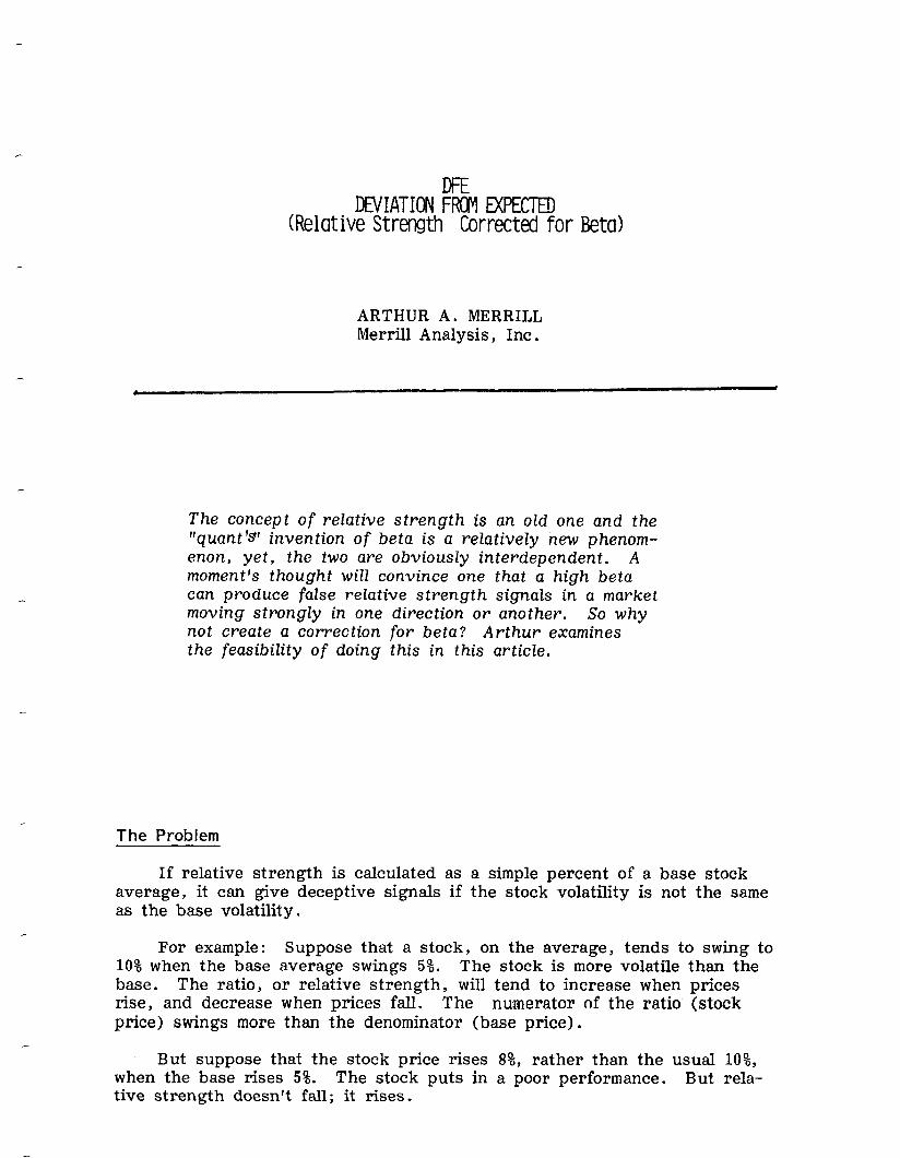
The concept of relative strength is an old one and the “quant’@ invention of beta is a relativezy new phenom- enon, yet, the two are obviously interdependent. A moment’s thought wiZ1 convince one that a high beta can produce false relative strength signals in a market moving strongly in one direction or another. So why not create a correction for beta? Arthur examines the feasibility of doing this in this article.

The Problem

If relative strength is calculated as a simple percent of a base stock average, it can give deceptive signals if the stock volatility is not the same as the base volatility.

For example : Suppose that a stock, on the average, tends to swing to 10% when the base average swings 5%. The stock is more volatile than the base. The ratio, or relative strength, will tend to increase when prices rise, and decrease when prices fall. The numerator of the ratio (stock price) swings more than the denominator (base price).

But suppose that the stock price rises 8%, rather than the usual lo%, when the base rises 5%. The stock puts in a poor performance. But relative strength doesn’t fall; it rises.

Suggested Solution :

To eliminate this beta effect, here is a proposal: use deviation-from- expected instead of a simple ratio.

The expected price would be a point on the line of regression; the deviation of actual price from this expected price would be a simple percentage above or below expected. Since prices tend to be geometric, the regression line should be fitted to logarithms. If you aren’t familiar with regression lines, you will find a brief explanatory note in Appendix A.

Example :

Two years of weekly data were tabulated for Warner Communications (WCI). The stock was a random selection. The stock price is in Figure 3; Relative Strength (price in percent of S&P 500) is in Figure 4.

A regression line was calculated each week to fit the data of the preceding 20 weeks. An example is in Figure 1. The method of calculation is outlined in Appendix B.

The deviation from the expected line is in Figure 5.

Results :

You will note some places in the charts where the Relative Strength and DFE give contrary indications.

To check the relative usefulness of Relative Strength and DFE, the curves were examined with the aid of a computer, and compared to the subsequent performance of the stock price. The method is as follows:

To generate “forecasts”, the current value of Relative Strength in each week of the two-year period was compared to an earlier value. The same technique was used for DFE. This is the equivalent of noting the direction of a moving average. For example, if a ten-week moving average is used, it will rise if the most recent statistic is higher than the statistic 11 weeks earlier; it will decline if the latest statistic is lower.

Using this method, 16 “forecasts” were generated for each week of the two-year period :

Is current relative strength higher or lower than the relative strength (1) in the preceding week (2) 2 weeks back (3) 3 weeks back (4) 4 weeks back (5) 5 weeks back (6) 6 weeks back (7) 7 weeks back (8) 8 weeks back

-22-

Is current Deviation From Expected higher or lower than DFE (9) in the preceding week (10) 2 weeks back ( 11) 3 weeks back (12) 4 weeks back (13) 5 weeks back (14) 6 weeks back (15) 7 weeks back (16) 8 weeks back

In addition, a forecast was generated by the level of DFE: (17) Is DFE in the highest 25% of all DFE in the

two-year period, or in the lowest 25%?

The success of the 17 forecasts was then scored by the performance of the stock pdce in the weeks following the forecast. Each forecast was scored right or wrong by ten different definitions of success:

Did Warner Communications close higher or lower 1. in the week following the forecast 2. 2 weeks after 3. 3 weeks after 4. 4 weeks after, and so on up to 10. 10 weeks following the forecast.

The significance of the results were checked by chi squared. The results are summarized in Figure 2.

Conclusions :

Note Figure 2. Simple relative strengthdemonstrated usefulness, with probably significant forecasts 8-to lo-weeks in the future. The most successful forecasts were made by comparing current relative strength with relative strength six or seven weeks earlier.

However, in this test, at least, DFE showed definite superiority. Several of the forecast averages were at the significant 1% level; two were at the highly significant 0.1% Ievel. The most successful forecasts were made by comparing current DFE with the level four weeks earlier.

-23-

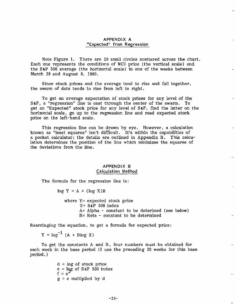
APPENDIX A “ExDected” from Rearession

Note Figure 1. There are 20 small circles scattered across the chart. Each one represents the conditions of WC1 price (the vertical scale) and the S&P 500 average (the horizontal scale) in one of the weeks between March 28 and August 8, 1980.

Since stock prices and the average tend to rise and fall together, the swarm of dots tends to rise from left to right.

To get an average expectation of stock prices for any level of the S&P , a “regression” line is cast through the center of the swarm. To get an “Expected” stock price for any level of S&P, find the latter on the horizontal scale, go up to the regression line and read expected stock price on the left-hand scale.

This regression Line can be drawn by eye. However, a calculation known as “least squares” isn’t difficult. It’s within the capabilities of a pocket calculator; the details are outlined in Appendix B. This calculation determines the position of the line which minimizes the squares of the deviations from the line.

APPENDIX B Calculation Method

The formula for the regression line is:

log Y = A + (log X)B

where Y= expected stock price X= S&P 500 index A= Alpha - constant to be deterimed (see below) B= Beta - constant to be determined

Rearringing the equation, to get a formula for expected price:

Y = log-l (A + Blog X)

To get the constants A and B, four numbers must be obtained for each week in the base period (I use the preceding 20 weeks for this base period. >

d = log of stock price e = 1~ of S&P 500 index f=e g = e multiplied by d

-24-

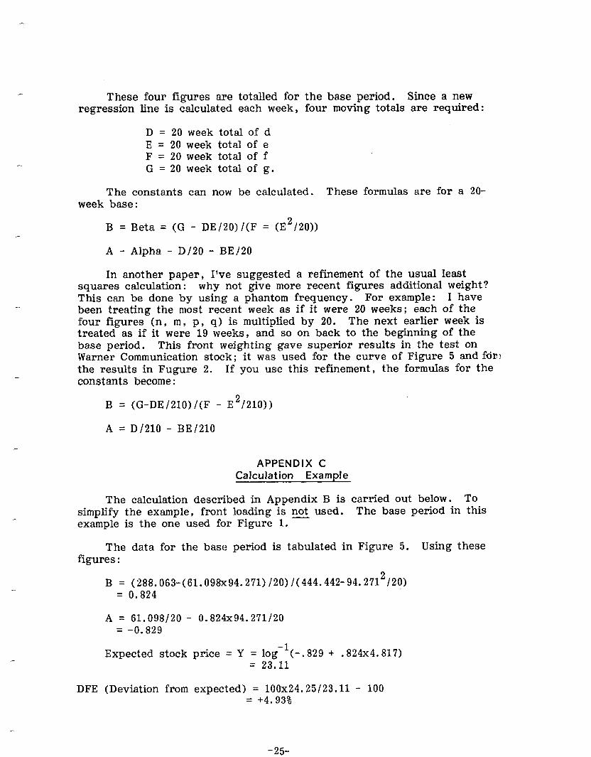
These four figures are totalled for the base period. Since a new regression line is calculated each week, four moving totals are required:

D = 20 week total of d E = 20 week total of e F = 20 week total of f G = 20 week total of g.

The constants can now be calculated. These formulas are for a 2O- week base:

B = Beta = (G - DE/20)/(F = (E2/20))

A- Alpha - D/20 - BE/20

In another paper, I’ve suggested a refinement of the usual least squares calculation : why not give more recent figures additional weight? This can be done by using a phantom frequency. For example: I have been treating the most recent week as if it were 20 weeks; each of the four figures (n, m , p , q) is multiplied by 20. The next earlier week is treated as if it were 19 weeks, and so on back to the beginning of the base period. This front weighting gave superior results in the test on Warner Communication stock; it was used for the curve of Figure 5 and fdr! the results in Fugure 2. If you use this refinement, the formulas for the constants become:

B = (G-DE/210)/(F - E2/210))

A = D/210 - BE/210

APPENDIX C Calculation Example

The calculation described in Appendix B is carried out below. To simplify the example, front loading is not used. The base period in this example is the one used for Figure 1. -

The data for the base period is tabulated in Figure 5. Using these figures :

B = (2S8.O63-(61.O98x94.27l)/2O)/(444.442-94.2712/2O) = 0.824

A= 61.098/20 - 0.824x94.271120 = -0.829

Expected stock price = Y = log-+-. 829 + .824x4.817) = 23.11

DFE (Deviation from expected) = 100x24.25/23.11 - 100 = +4.93%

-25-

25\

24-

WARNER GCIMMUNlCAllON

20 reeks 032800’000000

ACTUAL-&

DFE

-- SBP 500 - - FIG. I

FORECAST SUCCESS

Forecast success; weeks later:,

Relative Strength

forecasts:

current RS

compare‘d to

Rs inan earlier week.

We&e earuer:

1 2 3 4 5 6 7 8 9 lo I

DFE forecasts: 1

current DFE 2 P

compared to 3 S ss s PP

DFE in an 4 S S H*H P

earlier week. 5 S s s P

Weeks earlier: ~6 P P P

7

8

Key:

P=probably significant (5% level) Example: for a forecast of

S= significant (1% level) future price of WCI, the current

H=bighly significant (0. 170 level) DFE is compared with DFE four

weeks earlier. The forecasts were

Note: forecasts using the level scored right or wrong by noting

of DFE (in the highest or lowest whether WC1 closed higher or lower

25%) did not show significance. 6 weeks later. The results showed

high significance at the 0. 1% level.

(chi squared was 12. 50)

Fig. 2

--3&L

69

30

40

30

20

15. 1980 19at

SOY0 ,F Y . I ,I J . E 0 n D

1960 1981

FIG.4

-27-

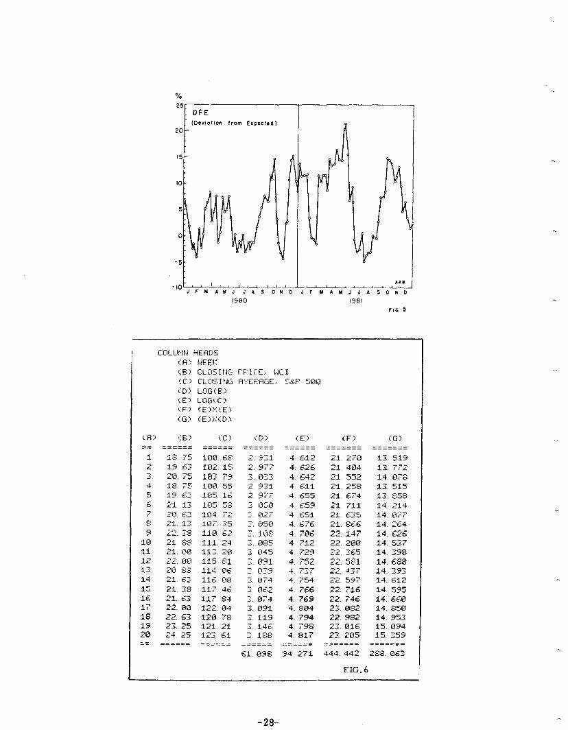
% 25

LIFE from Expected)

20

I5

IO

5

0

-5

t I

1980 I981

FIG 5

-28-

LOGMITl+lIC F’OINT ND FIGURE CHARTS

ARTHUR MERRILL Merrill Analysis

Arthur is famiZiar with both the old and the modern. Here he applies a new twist, a logarithmic scale, to an old technique, point-and-figure sharts. As usual, the results are fascinating.

Why logarithmic? Consider a trend line on an arithmetic chart, rising at the rate of one point per week, from 10 at the left hand end of the chart to 62 at the right hand end. At the left hand end the rise is 10% per week; at the right hand end the rise is only 1.96% per week. The arithmetic scale has distorted the trend line.

A logarithmic scale agrees with the geometric nature of the stock prices. A trend line rising at 10% per week at the left hand end of the chart is still rising at 10% per wwk at the right hand end of the chart.

In the usual point and figure chart, the filter is designated in points, and any swing smaller than this filter is ignored. In the logarithmic point and figure chart, the filter is designated in percent, rather than in points. In Figure 1 the filter was 10%.

The scale in a logarithmic chart isn’t uniform, so the rises and declines in a longhand chart can’t be followed by uniform columns of x or 0. Instead, horizontal lines can be drawn to follow the progress of prices up or down. If the chart is drawn by computer, price changes can be approximated by the usual X or 0, as in Figure 1.

The ordinary interpretations of a point and figure chart should be the same with arithmetic or logarithmic. An exception is the use of the width of a

-29-

base formation as a measure of probable rise. The horizontal scale is arithmetic; the. vertical scale is logarithmic, so direct measure isn’t possible . Instead, if the number of swings is expected to translate into points rise, these points must be measured off against the log scale.

Figure 1 was generated by a Radio Shack microcomputer. If you would like to see the program, please write.

The advantages of a log chart are substantial:

1. Trend lines are undistorted. 2. Changes at the top and the bottom of a chart are comparable. 3. Charts using the same filter are comparable.

-3o-

.

MERRILL HNALYSIS IW. SCHLUPIBERGER

.

-31-

,

intentionally blank

- 32-

IN PRAISE OF PANICS

RICHARD C . ORR, PH.D. NANCY A. ROONEY

Contratrend, Inc.

Technicians, as this article points out, are wont to use terms imprecisely. Here the authors offer precise definitions of the much-abused terms, “panic” and “selling climax” and test the historical record following such occurrences. Dick Orr, a prolific contributor to the Journal, is an MTA member and former Professor of Mathematics at the State University of New York, Recently, together with his co-author, Nancy Rooney, he has started his own service, Contratrend, Inc.

I. Introduction

Everyone talks about a selling climax but not everyone agrees upon the conditions necessary for such a climax to occur. Therefore, from time to time, arguments will arise between technicians as to whether the price and/ or volume action of a particular index did or did not constitute a selling climax. A perfect example would be the market behavior of September 25- 28, 1981. This paper will not resolve all outstanding arguments relating to selling climaxes. What we do propose to accomplish here is to provide our reader with a very simple technique which has an admirable 35-year record of signaling market bottoms. This study uses the S & P 400 Industrials as the market index. Our results would vary somewhat if one used the S & P 500, the D .J.I .A. or the N .Y .S .E. Composite, but the basic ideas presented here pertain to all of these broad indices.

It should be pointed out that these techniques do not apply to individual stock-price action without considerable theoretical modifications. This is a point which is often missed by some technicians. The use of techniques interchangably between market indices and individual stocks is, at least some of the time, inappropriate. At Contratrend, we are in the business of forecasing fairly substantial six-month moves in stocks which are oversold or, in some instances, overbought, It is possible to combine our individual-stock forecasts in order to get a profile of the entire market, but this is a one-way street. Except in extreme cases, a general technique of the type described below will have little use when applied to a particular stock.

-33-

Two caveats are worth mentioning. First, no indicator is perfect. What we present here is an indicator with a high probability of success based on a fairly long history. It gives few incorrect signals, and it misses few signals, but it is not infallible. If it were, then the second caveat would come into play, that is, if any indicator becomes too popular, it is doomed to failure (at least until it loses some of its popularity). To couch this second caveat in the mathematical jargon of game theory: if a player develops a winning strategy for a given game, then it remains useful only if the other players don’t discover and adopt it. If all the players use the same strategy, the advantage is lost to all.

One of the problems we face constantly as technicians is an inconsistency in our definitions for the terms we use. What is a bull market? What does “intermediate-term” mean? If one is to measure the performance of an indicator which is claimed to be effective in signaling major bottoms in the market, then the notion of a major bottom must be defined in unambiguous terms. There are numerous good candidates for such a definition. The key is to remain consistent in one’s usage. We will present our own definition later in this paper. We begin, -however, with another definition. A panic is defined to be a ten-percent move either way in the daily closing pr!f an index in less than a one-month period. Volume is not taken into consideration . A period of one month is used rather than, say, 21 trading days because historically not all holiday-free weeks have consisted of 5 trading days. Under our definition a panic occurs either within a given month (e.g.: November, 1948) or across two months (e. g. : July to August, 1966). In the latter case, the date of the completion of a ten-percent move in the second month must be smaller than the date of the initiation of the move in the first month. Therefore, July 14 to August 12 would be acceptable, but July 10 to August 16 (or even July 10 to August 10) would not be less than one month and, hence, would be unacceptable. We will consider here only selling panics in the S & P 400, namely, a ten-percent drop in that index within a period of less than one month.

Il. Selling Panics and Major Bottoms : 1946-1981

The first table liclsts all drops in the S & P 400 index of at least ten percent in less than one month. A signal is considered to be given at the close of the first day on which these conditions have been met. Any subsequent time period to be considered for another possible signal must begin after this day. In other words, multiple signals are possible (see 1974, for example), but the time periods for thse signals may not share even one common day. The date and closing signals may not share even one common day. The date and closing price for each signal are listed, together with the closing price for each signal are listed, together with the closing price exactly one year later and the extreme percentages gained and lost within the subsequent year.

- 34-

Notice that, of the 21 signals for which we have a complete one-year history, the low for the next year preceeded the high for the next year in 19 cases. This is at least as important as the actual percentages in the fourth and fifth columns in Table I. Certain statistics we could derive from the table would be misleading, so we will summarize our results very conservatively. The average percentage gained from “buying the index” with equal investments on each signal and holding for a period of exactly one year is 18.26%. If one wishes to obtain an accurate compound growth rate for this investment technique, we would suggest that., when one has more than one signal within a year, that the holding period simply be extended by exactly one year from the next signal, Then, for example, we have a buy signal on November 20, 1973 which remains in effect until August 8, 1976, This approach seems more reasonable than one involving multiple signals, if one is interested in compound growth rates. For the above period, the compound growth rate over the approximately 14 years for which we have signals in force is 12.4%. No assumption is made about alternative investments over perials of time (approximately 21 years) when no signal is in force.

In Table 2, we look at the record of the same “panics”, this time from a three-year perspective. In all cases, except for the two signals in 1946, the three-year low preceeded the three-year high. This favorable ordering exists, even in 1973 when the signal was definitely a bad one. The aver- ate percentage gain to the three-year high is 45.8%, while the average percentage loss to the three-year low is 10.0%.

Thus far, we have seen that the track record of the panic selling indicator is excellent. But are any errors of omission present? Are there major market bottoms for which no signal is given? In order to answer that question it is necessary to define what is meant by extremes in a market index. Again, many definitions are possible. The key to a good one is ease of use and lack of ambiguity. We define a major bottom in an index to be a closing price in that index over some time interval which is the lowest price in the interval and is at least 20 percent lower than both some previous day and some subsequent day in that interval. There is no’ time limit imposed in this definition. In other words, if an index drops at least 20 percent to some minimum value and then rises at least 20 percent above that value we will call that minimum value a major bottom. We define a major top analogously : a 20 percent rise followed by a 20 percent fall in an index constitutes a major top.

In Table 3, we have listed all major tops and bottoms in the S & P 400 index over the last 35 years. As of this writing it is still too early to tell if the September 25, 1981 low was, in fact, a major bottom. Also listed in this table are the date and closing price of the nearest selling panic either before or after each major bottom. Although the sample size is small, we see that, in all cases, there is a signal within about ten percent of each major bottom, in some cases much closer l In four of the seven cases the signal preceeds the actual bottom by only days, in a fifth case by five weeks and in a sixth case by five months. Only in the seven case, in 1978, did the signal actually follow the major bottom, in this instance by about eight months.

:h

-35-

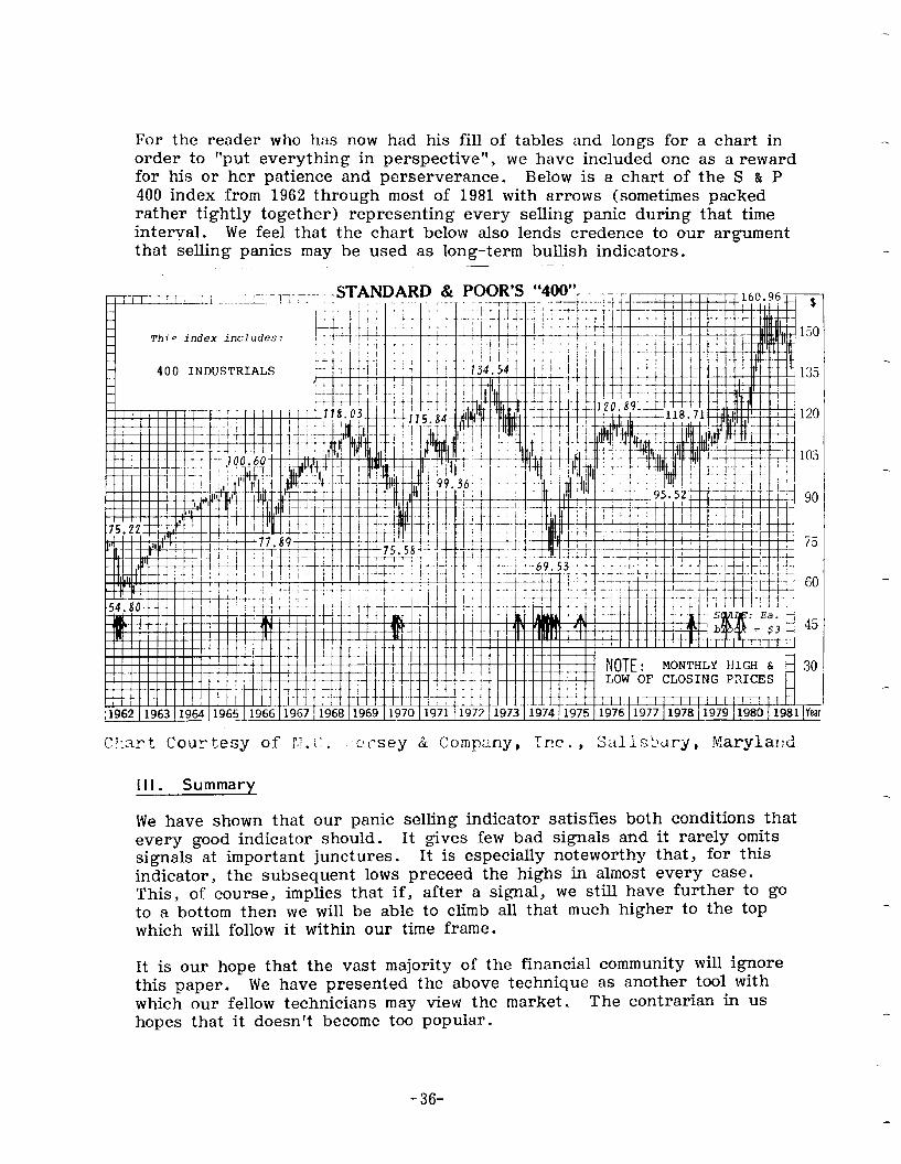
For the reader who has now had his fill of tables and longs for a chart in order to “put everything in perspective”, we have included one as a reward for his or her patience and perserverance. Below is a chart of the S & P 400 index from 1962 through most of 1981 with arrows (sometimes packed rather tightly together) representing every selling panic during that time int eryal . We feel that the chart below also lends credence to our argument that selling panics may be used as long-term bullish indicators.

index includes:

400 INDUSTRIALS

III. Summary

We have shown that our panic selling indicator satisfies both conditions that every good indicator should. It gives few bad signals and it rarely omits signals at important junctures. It is especially noteworthy that, for this indicator, the subsequent lows preceed the highs in almost every case. This, of course, implies that if, after a signal, we still have further to go to a bottom then we will be able to climb all that much higher to the top which will follow it within our time frame.

It is our hope that the vast majority of the financial community will ignore this paper. We have presented the above technique as another tool with which our fellow technicians may view the market. The contrarian in us hopes that it doesn’t become too popular m

- 36-

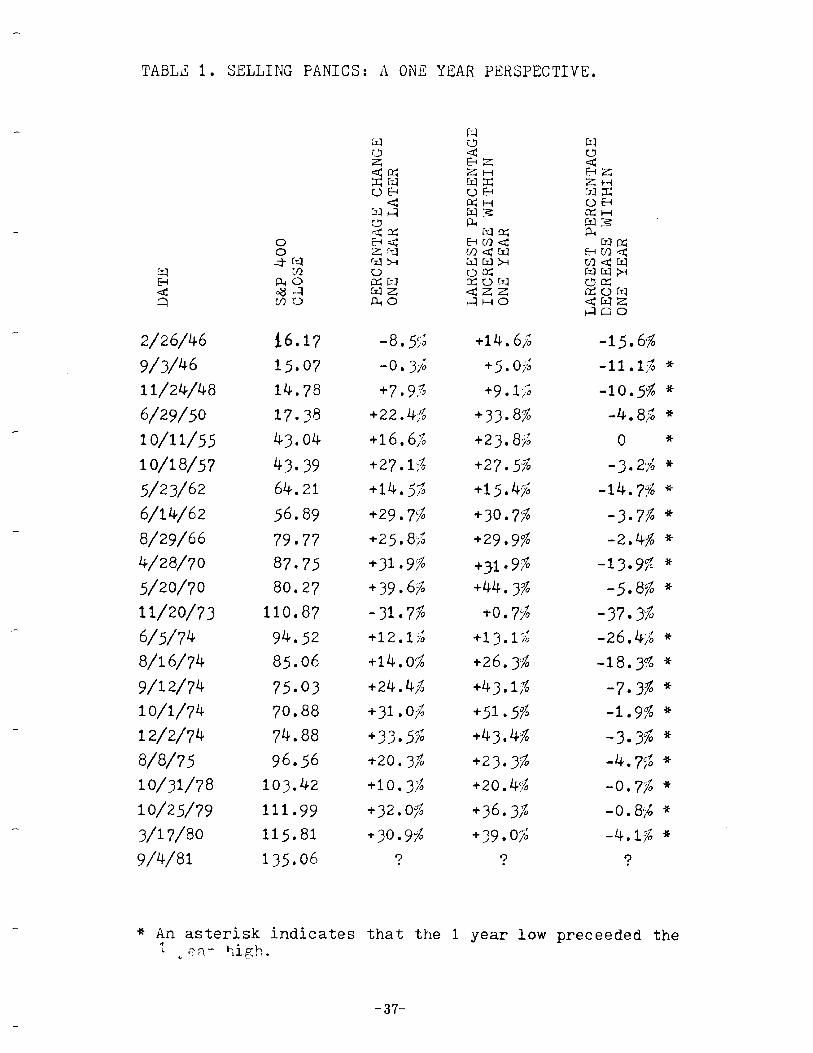
TABLE 1. SELLING FANICS: A ONE YEAR PERSPECTIVE.

2/26/46

g/3/46 H/24/48

6/29/50

1 O/l l/55

10/18/57

5/23/62 6/14/62

8/w/66

4/2a/70

5/20/70

1 l/20/73

6/5/74

8/l b/74

S/l z/74

1 o/1/74

I. z/2/74

B/8/75

1 o/31/78

10/25/79

3/l 7/80

9/4/81

i6.17 -8.5:‘;

15.07 -0.3;

14.78 +7.g.s

17.38 +22e4j%

43.04 +16,6,S

43.39 +27,l;‘la

64-. 21 +14.5$

56.89 +29.7%

79.77 +25.8$

87.75 +31.9$

80.27 +3g.6%

110.87 -31.7%

94d2 + 12 . 1 ,f

85.06 +14.0$

75.03 +24.4$

70.88 +31,0$

74.88 +3395%

96.56 +20.3%

103.42 +10.3$

111.99 +32.0%

115.81 +30.9%

135.06 ?

+14.6$

+5.0$

+9.1$

+33.8%

+23,ajs +27.5$

+15.4$

+30.7$

+2999%

+31 l 9% +44.3%

+0.7$

+13.1;6

+26.3,%

+43.1%

+51.5%

+43.4%

+23* 3% +20.4$

+36.3$

+39.0$

?

-15.6%

-ll.l;$J *

-10.5% *

-4. a,% *

0 *

-3.2g *

-14.7% *

-3.7% *

-2.4% *

-13.9% *

-5.8% *

-37.3% q&4$ +t-

-18.3% *

-7.3% *

-1.9% *

-3.3% * -4.7% *

-0.7% *

-0.85 *

-4.1-g *

?

* An asterisk indicates that the 1 year low preceeded the 4 i. 92 - *;igh. c .

-37-

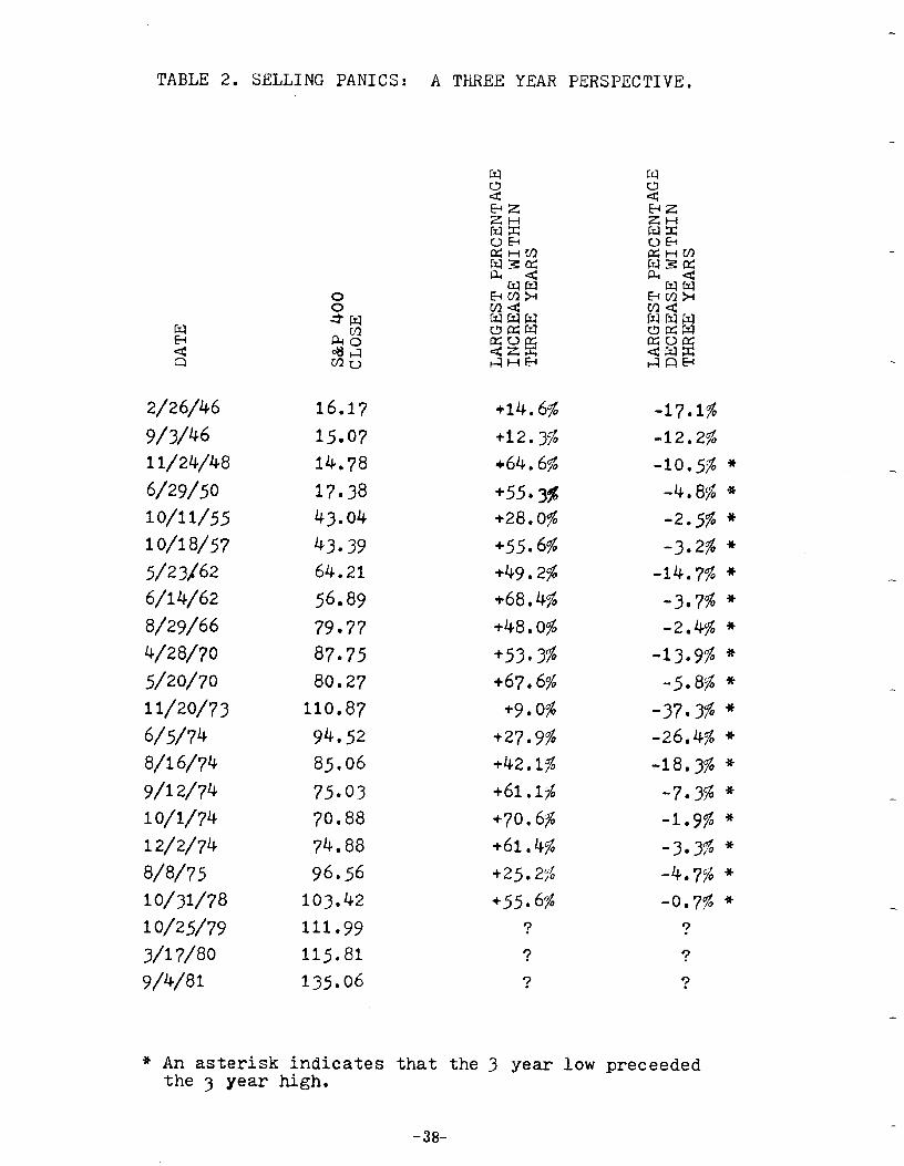
TABLE 2. SELLING PANICS: A THREE YEAR PERSPECTIVE.

2/26/46 16.17

9/3/46 15.07 11/24/48 14.78

6/29/s 17.38

lo/w55 43.04

10/18/57 43.39

5/23/62 64.21

6/14/62 56.89

B/29/66 79.77

4/28/70 87.75

j/20/70 80.27

11/20/73 110.87

6/5/74 94.52

a/l 6/74 85.06

9/l 2/74 75.03

1 o/1/74 70.88

12/2/74 74.88

m/75 96.56

10/31/78 103.42

1 O/25/79 111.99

3/l ?/80 115.81

9/4/81 135.06

+14.6%

+12.3$

+64.6$

+55*3$

+28.0%

+55.6%

+49.2$

+68,4%

+4&O%

+53a 3% +67.&/o

+9.0%

+27.9$

+42.1$

+61.1$

+70,6%

+61.4%

+25.2%

+55.6%

?

?

?

-17.1%

-12.2%

-10.5% *

-4.8% *

-2.5% +

-3.2% *

-14.7% *

-3*7% * -2.4% *

-13.9% *

-5.&$ *

-37.3% * -26.4% *

-18.3% *

-7.3% *

-1.9% *

-3.3% *

-4.7% *

-0.7% *

?

?

?

+ An asterisk indicates that the 3 year low preceeded the 3 year high.

-38-

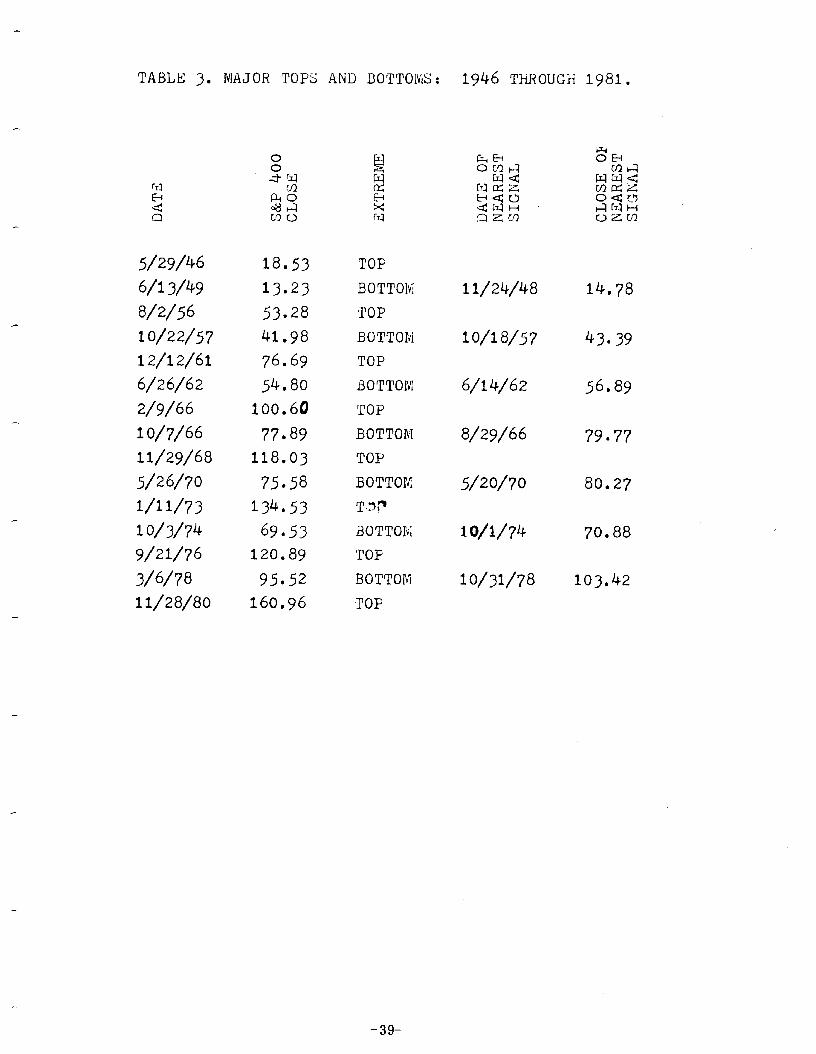
TABLE 3. MAJOR TOPS AND BOTTOMS: 1946 THROUGH 1981.

5/29/46 18.53 TOP

6/13/49 13.23 BOTTOM

8/2/56 53.28 TOP

10/22/57 41.98 BOTTOM 12/12/a 76.69 TOP 6/26/62 54.80 BOTTOM

2/9/66 100.68 TOP

10/7/66 77.89 BOTTOM

H/29/68 118.03 TOP

5/26/70 75.58 BOTTOK

l/l r/73 134*53 TZp

10/3/74 69,53 BOTTObI

9/21/76 120.89 TOF

3/6/78 95.52 BOTTOM

U/28/80 160.96 TOP

H/24/48 14.78

10/18/57

6/14/62

43.39

56.89

B/29/66 79.77

5/20/70

WV74

10/31/78

80.27

70.88

103.42

-39-

intentionally blank

-4o-

THE WEKLY RULE IN (XIPTWDITY FUI-LJRES TRADING

JOHN J. MURPHY JJM Technical Advisors

John Murphy was a speaker at the 1982 MTA Seminar and this article is based, in part, on his speech at that seminar. He has also been a speaker at one of our regular monthly meetings. John is the president of JJM Technical Advisors, a CFTC-registered commodity advisory firm. He has been Director of Commodity Research for Brascan International and has been associated with Merrill Lynch and CIT Financial Corporation.

With the introduction of computer technology over the past decade, a considerable amount of research has been done on the development of technical trading systems for use in commodity-futures markets. These systems are mechanical in nature, which means that the trader must be disciplined enough to follow the system’s signals. The temptation which must be resisted is to “override” the computer signals because they dis- agree with the trader’s judgment of the market, or to abandon or modify the system during the inevitable periods of adversity.

These systems have become increasingly sophisticated over the years. At first, simple moving averages were utilized. Then double and triple crossovers of the averages were added. Then the averages were linearly weighted and exponentially smoothed. More recently, advanced mathematical and statistical techniques, such as linear regression, have ‘been applied.

Most of these systems are trend-following, which means that their purpose is to identify a trend that has already been established, and then to trade in the direction of that trend, either on the long or short side, until the system indicates the trend has reversed.

-41-

With the increased fascination with fancier and more complex systems and indicators, however, there has been a tendency to overlook some of the simpler techniques that work quite well and have stood the test of time. This article is about one of the simplest of these techniques -- the weekly rule.

In 1970, a booklet entitled the Trader’s Notebook was published by Dunn & Hargitt’s Financial Services in Lafayette, Indiana. The best known mechanical systems of the day were computer-tested and compared. Their final conclusion was that the most successful of all was the “four-week rule” developed by Richard Donchian. who is generally considered one of the pioneers in the early development of mechanical methods.

The system is incredibly simple:

1. Buy and cover short positions whenever the price exceeds the highs of the four preceding full-calendar weeks’ range.

2. Liquidate long positions and sell short whenever the price falls below the low of the four preceding calendar weeks.

The system, as it is presented here, is continuous in nature, which means that one is always in the market, either long or short. As a general rule, continuous systems have a basic weakness, which is their tendency to stay in the market and get “whipsawed” during trendless market periods. Trend-following systems do not work well when markets are in a sideways, or “non-trending”, mode, which may be the case for as much as a half to a third of the time. One way to make this system “non-continuous” is to use a shorter time span, for example, a one-or two-week rule for liquidation purposes. Therefore, a four-week “breakout” would be necessary to initiate a new position, but a one-or two-week signal in the opposite direction would warrant liquidation of the position. The investor would then remain out of the market until a new four-week “breakout” is registered.

The inherent logic of the system is based on sound technical princi- pies . It is mechanical, so that human judgment and emotion are eliminated. Since it is trend-following, it virtually guarantees participation on the right side of every important trend. It is also structured to follow the often quoted maxim of successful commodity trading, which is to “let profits run, while cutting losses short”. Another feature, which should not be over- looked, is that this method tends to trade less frequently, so that commissions tend to be lower. This is one reason why this particular sys$em is popular among money managers and not so popular among brokers. One other point is that this can be easily implemented without the aid of a computer.

The main criticism of this approach is the same one that is leveled against all trend-following approaches, namely, that it does not catch tops or bottoms. It is beyond the scope of this article to argue the merits of trend-following systems. Suffice it to say here that large profits in

- 42-

commodity trading are generally achieved by participation in major trends, which is the basis for this approach.

For the purpose of this article, the examples shown will present the “four-week rule” pretty much in its original form. In reality, however, there are many adjustments and refinements which can be employed. For one thing, the rule does not have to be used as a system. It can be employed simply as another technical indicator to identify breakouts and trend reversals.

The length of the weekly rules can be adjusted to different markets. Some research done in this area suggests that trading results can be opti- mized by varying the number of weeks used in different markets. For example, it has been s.uggested that a two-week rule works best in the livestock markets, while a six-week rule may work best in copper.

In certain types of market situations, the time period employed could be expanded or compressed in the interests of risk management and sensitivity . For example, in lower-priced markets, with relatively low volatility, the time horizon could be expanded. In higher-priced markets, however, with higher volatility, the time horizon, or number of weeks employed, could be shortened to increase the sensitivity of the method.

For some reason, which I suspect has to do with the principle of harmonics in cycle analysis, adjustments to the four-week rule seem to work well when the beginning number is divided or multiplied by two. Therefore, to shorten the horizon, we go from four to two. To lengthen it, we go from four to eight. Since this method does combine price and time, there’s no reason why the principle of harmonics in cycles analysis should not play a role. The principle of harmonics states that each cycle is related to its neighboring cycles by a small whole number which is usually two. So the tactic of dividing a weekly rule by two to shorten it, or multiply it by two to lengthen it, does have cycle logic behind it.

The problem with attempting to optimize the four-week rule, adding all of the above-mentioned refinements, is that the user begins to lose the system’s greatest strength, which is its simplicity. Despite constant attempts to improve on the results over the years, I find myself inevitably drawn back to the original system. Since this rule is meant to be simple, perhaps it is best addressed on that level. Probably the most apt descrip- tion of the four-week rule is that it is simple, but it works.

Since so many commodity-futures markets have been in major down- trends, it is not difficult to choose from among many excellent recent examples of the application of the weekly rule. While not trying to over- sell the technique, a quick glance at the examples shown and several other futures charts found in any good chart service should pretty much speak for itself.

-43-

The above Heating Oil chart shows the system short for the entire August / March decline. The system then went long at about 78 cents. The dotted lines show points where earlier liquidation could have occurred with a two- week rule. Using just the four-week rule and taking just the last two signals, the system made over 20 cents on the downside and over 10 cents on the upside.

_: ;VALUE LINE AN. WT. 1982 - K.C. : x UC” IO.ILON,lY “NE . Ka Pawn

The Value Line Stock chart at left shows a “buy” near 125 in late March, and then a reversal to the short side at 130 in mid-May. The system remained short through June.

.-

I I A”G I SCPT 1 0c-r / “0” DEC. I JAN I FE8 i U&R APa I HI” I JUPiE I --

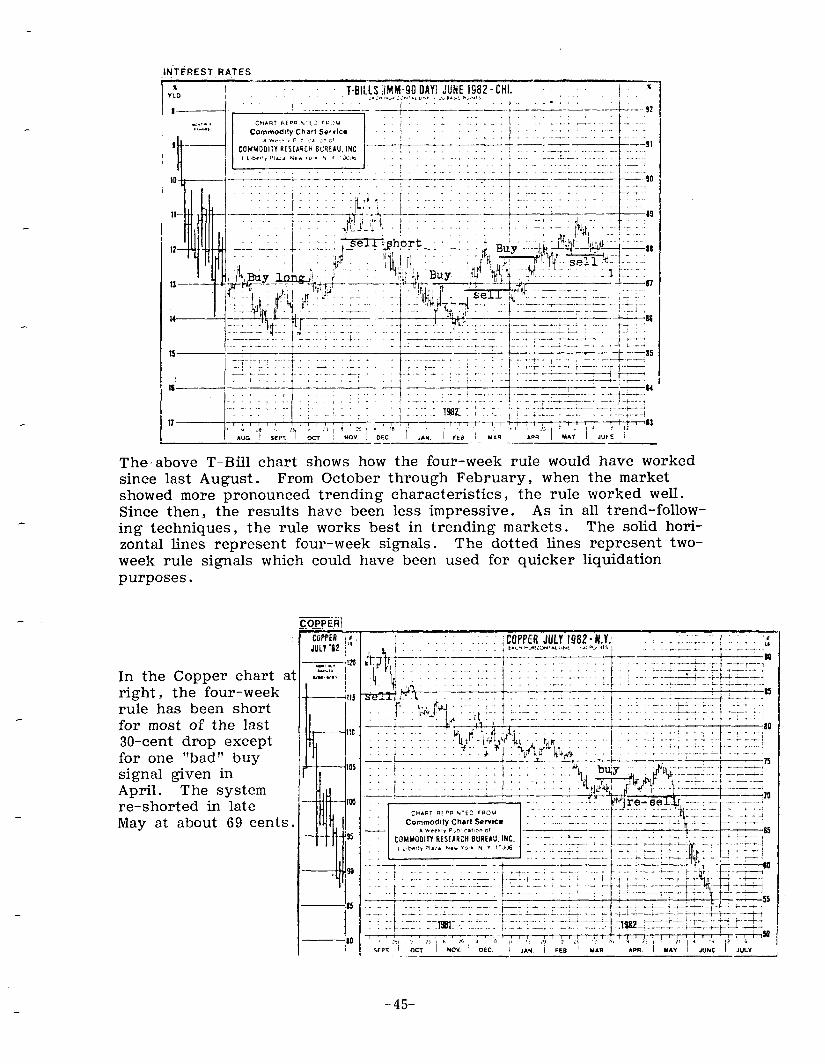
The,above T-Bill chart shows how the four-week rule would have worked since last August. From October through February, when the market showed more pronounced trending characteristics, the ruIe worked well. Since then, the results have been less impressive. As in all trend-following techniques, the rule works best in trending markets. The solid horizontal lines represent four-week signals. The dotted lines represent two- week rule signals which could have been used for quicker liquidation purposes.

Z@@ii

COPPER II JULV ‘32 1”

In the Copper chart al right, the four-week rule has been short for most of the last 30-cent drop except for one “bad” buy signal given in April. The system re-shorted in late May at about 69 cents.

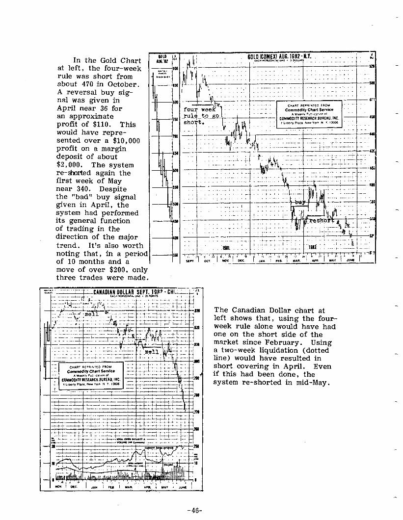
In the Gold Chart at left, the four-week rule was short from about 470 in October. A reversal buy signal was given in April near 36 for an approximate profit of $110. This would have represented over a $10,000 profit on a margin deposit of about $2,000. The system re-&orted again the first week of May near 340. Despite the “bad” buy signal given in April, the system had performed its general function of trading in the direction of the major trend. It’s also worth noting that, in a period of 10 months and a move of over $200, only three trades were made.

6010 ICOMEXI AU6.1982 - 1.1.

--- - CANADIAN DOLLAR SEPT. 19P7 - CltL-&“, UC” tu3w.ouTAl “kt . x) rcwR 78 -

The Canadian Dollar chart at left shows that, using the four- week rule alone would have had one on the short side of the market since February. Using a two-week liquidation (dotted line) would have resulted in short covering in April. Even if this had been done, the system re-shorted in mid-May.

-46-

THE INN-TiiEORY INDEX

WILLIAM DiIAN N I Wellington Management Company

Bill DiIanni, former editor of this Journal, is well-known for creative ideas. Why, he reasons here, should the Dow Theory require two indicators, the lndus trials and the Transports? In this article, he suggests a “Dow- Theory Index”, a single indicator which embodies at least some of the traditional Dow-Theory concepts.

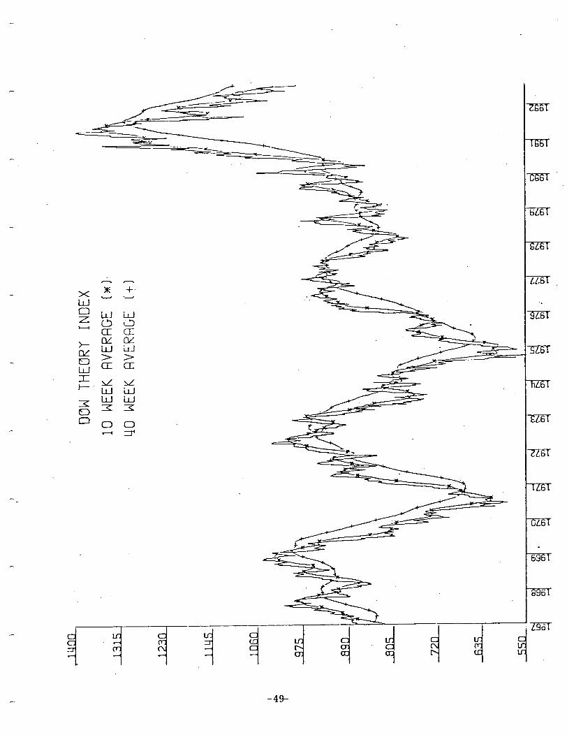
This index is an effort to put the traditional “DOW Theory” on one line, instead of using two separate averages with its principles of confirmation and non-confirmations.

With all of the various averages and indicators used by market analysts these days, they certainly don’t need one more. But we have experimented with this one for a while and found that it might be helpful as an ancillary indicator. As one studies the attached chart, one can see some interesting periods when the theory might have been helpful in determining market turns and even identifying areas of likely support and resistance.

The construction of the indicator is rather simple, and not totally scientific. One works with the weekly close of the Dow Jones Industrial Averages and the weekly close of the Dow Jones Transportation Average. In order to give equal balace to both averages, we multiplied the Transports by 4, then the two figures are added together. Even though it is not necessary, we have divided the resulting figure by 2 to arrive at a single number close to the Dow Industrials itself.

For example :

Industrials (900) + Transports (300 x 4) = 1o5o 2

We have also constructed a 10 week and 40 week moving average and plot them with the raw figures for trend control. Simple enough?

-47-

We want to stress that this index should not be considered a substitute for the time honored Dow-Theory Principles of Charles Dow, William Hamilton and Robert Rhea. It should be used as an aid to other tools. For even the early Dow theorists themselves were quick to admonish that their theory was not infallible. We reiterate their admonitions wholeheart- edly . It is only that at certain times, another graph such as this one may clarify certain confusing periods, or strengthen one’s conviction at crucial junctures.

One example of such a period was the all-time high breakout of the Dow Industrials during the December 1972-January 1973 period. This was not confirmed by the Transports using standard Dow-Theory rules. It was even more evident in our Dow-Theory Index, as the weakness in the Trans- ports failed to produce a “new high” in the Index. Furthermore, momentum as measured by the lo-week and 40-week moving averages was in the process of a serious roll-over. What followed was the severest bear market since the thirties, ending in late 1974.

At the end of 1974, standard Dow-Theory Principles called for a traditional low when the Transports did not confirm the minor new low in the Indus- trials. This non-confirmation was equally reflected in our Index as no new low was recorded during the test of the September-October 1974 lows.

There are many areas of interest, so let us point out a few more. Before the Bunker Hunt decline, the Index reached resistance at the 1968 high-- nearly matching it to the penny. Then at the low end of its trading range and at the height of the selling climax, it again failed to break its previous support level. An extended uptrend began, the Transports,

and, because of the strength in

margin. the Dow-Theory Index went on to all-time highs by a wide

This record new high cleared all comparable highs going back to 1966. It ran into trouble during the second quarter of 1981 and began to take on distribution-type characteristics during the summer of 1981, as the lo-week moving average rolled over the price. A decline began. Is it a correction, or has an extended bear market begun?

At this point in time (August, 1982) it looks very much like a severe correction. According to this Index, the market is experiencing a three-step decline which has undercut the September-October 1981 lows, and tested the area of breakout which is represented by the series of highs traced out since 1966. 1982 should be quite interesting. A bottoming pattern confirmed by negative sentiment around the 900-1000 zone of this Index could establish the end of the current decline. Obviously, (at this writing) the jury is still out. And, one should wait for a bona fide reversal in the price structure before prematurely committing.

As stated at the outset, this Index is not intended to replace traditional Dow- Theory Principles. period

But at times, it may be helpful in clarifying a confusing -- especially during fast moving markets. Empirically, it seems to

work . . . and isn’t that what it’s all about?

-48-

intentionally blank

-5o-

PERFOFl’VVKE SIPUATION OF TECttNICAL ANALYSTS Second Year, Market Timing

CLINTON M. BIDWELL & PETER BACKUS

Professor Clinton BidwelZ, some two and a half years ago, cooperated with the MTA in an empirical test of technical analysis. Conclusion : It worked. This article is a report on a second similar test, conducted independently of the MTA, aZthough with certain members as individual participants. The bottom line is not all that dissimilar. Professor Bidwell is Associate Professor of Finance at the College of Business Administration, University of Hawaii. Peter Backus is a computer consultant for Pineapple Computer.

Introduction

This study is a continuation of a “real time” performance simulation of technical analysts. Despite certain communication problems in the initial study between Professor Bidwell and the 37 participants, the results over the one-year June 1977 to June 1978 test period were published in the MTA Journal, November, 1979. The original study contained two separate simulation forms; one of market timing (“A Game”) wherein the participants chose to buy, sell, or sell short a market index fund (or be invested in Treasury Bills), the second (“B Game”) involving individual securitv selection, long or short. The results of the original simulation tended to support the timing and stock selection ability of the participating analysts, especially in the second form of the simulation (stock selectivity). Twelve of the volunteer technical analysts participated in the “A Game”, 25 in the “B Game”.

A second year studv test was conducted, although not under the auspices of the Market Technicians Association. The purpose of this second study was to determine whether or not there would be evidence of continuity in market timing ability. The second simulation form involving stock selection was abandoned as too time consuming for the technical analysts participants in favor of the market timing simulation mode (“A Game”).

-51-

The Second Year

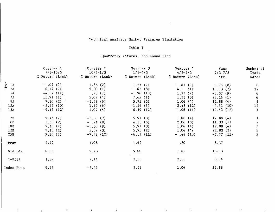
Twelve participants, all of whom had participated in the original A or B simulation, volunteered for this followup study. The one-year test period extended from July 3, 1978 to July 3, 1979.

As in the first study, the “A Game” format allowed purchase, sale, short sale, and buy cover of a no-load index fund (First Index Investment Trust, Vanguard Group). The Fund could be bought or sold short in any percentage up to 100% of each paper portfolio. Quarterly Fund cash dividends were converted into an increased number of shares if the participant was long, a decreased number if short. The initial paper portfolio was again $l,OOO,OOO with margin not permitted and no commissions charged as the Fund is a no- load Fund.

An important improvement was made in communications between the analysts and “game headquarters”. Confirmation was sent after every trade acknowl- edging receipt of the new instructions and reporting the analysts’ new portfolio position back to him. In addition, each participant received a quarterly evaluation showing his relative performance for the period. At the outset, in absence of countervailing instructions, each portfolio was presumed 100% long the index fund. In the first study the presumed initial portfolio position was 100% Treasury Bills.

Results

In contrast to the low market (index fund) return of the first study of 2.96%, the index fund in the second test period provided a return of 12.88%, or almost 4% above the Treasury Bill rate. The stronger stock market environment made it more difficult for the analysts to outperform a naive buy- and-hold strategy.

.

Table I presents the relative ranking, return results, and number of trades for the second year simulation.

Three of the 12 participants, 7A, 13B, and 3A, outperformed the market returns as measured by the performance of the First Index Fund. 7A’s returns of 28.26% more than doubled that of the Fund’s, while the returns of 13B and 3A were over 50% greater. In addition, three participants chose a buy and hold policy over the 12 months thus equalling the Fund’s perform- ante .

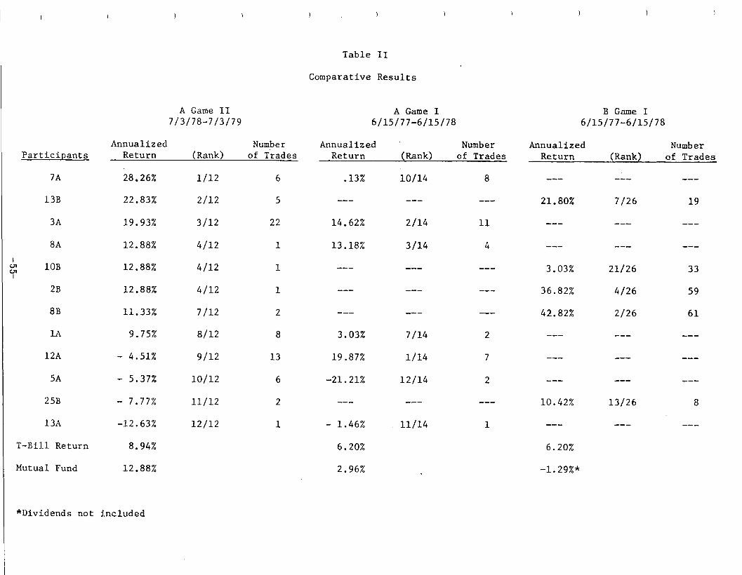
Comparative Results

Table II presents the performance results of this study in comparison with the performance results for the participants analysts in the first study. Two of the three outstanding performers also did quite well in the prior test period.

-52-

Conclusion

The author firmly believes that academic tests involving computer simulation of one or another technical tool does not effectively test the abilities of technical analysis as practiced. Most studies of fundamental analysis have focused on the results of security recommendations or professionally managed pools of money, rather than a computer simulation of one or another of their quantifiable inputs. Technical analysis should be similarly adjudged. These two studies, in spite of their imperfections, are an attempt to remedy this. A tentative conclusion, in viewing the results of both studies, is that technical analysis is as effective as the ability of the individual practitioner . Participants 13B and 3A evidenced outstanding market timing ability in both studies over two dissimilar market periods.

Author’s footnote : I am deeply appreciative to those analysts who participated actively in this endeavor. Regardless of how each of you did, hopefully by focusing on an historical record of your performance you will benefit through continued improvement of technique and improved application.

-53-

13A

3R ii

10B 13B 25B

Mean 4.49 1.08 1.65 .80 8.37

Std.Dev. 6.68 5.43 5.00 1.62 13.03

I T-Bill

Index Fund 9.16 -3.39 5.91 1.06 12.88

Quarter 1 Quarter 2 Quarter 3 Quarter 4 Year Number of 713-1013 10/3-l/3 l/3-4/3 413-713 7/3-713 Trade

% Return (Rank) % Return (Rank) % Return (Rank) % Return (Rank) etc. Dates

- .07 (9) 7.68 (2) 1.35 (7) - .65 (9) 6.17 (7) 9.20 (1) - .65 (8) 4.1 (1)

-4.87 (11) .23 (7) -1.96 (10) 1.22 (2) 11.91 (1) 5.07 (4) 7.65 (1) 1.33 (3)

9.16 (2) ' -3.39 (9) 5.91 (3) 1.06 (4) -2.67 (10) 1.92 (6) -1.54 (9) -2.48 (12) -9.16 (12) 4.07 (5) -6.59 (12) -1.06 (11)

9.16 (2) -3.39 (9) 5.91 (3) 1.06 (4) 12.88 (4) 5.50 (2) - .71 (8) 4.13 (6) 2.06 (8) 11.33 (7) 9.16 (2) -3.30 (9) 5.91 (3) 1.06 (4) 12.88 (4) 9.16 (2) 5.09 (3) 5.95 (2) 1.06 (4) 22.83 (2) 9.16 (2) -9.42 (12) -6.31 (11) - -44 (10) -7.77 (11)

1.82 2.14 2.35 2.35 8.94

Technical Analysts Market Training Simulation

Table I

Quarterly returns, Non-annualized

9.75 (8) 8 19.93 (3) 22 -5.37 (9) 6 28.26 (1) 6 12.88 (4) 1 -4.51 (10) 13

-12.63 (12) 1

Participants

7A

13B

3A

8A

I 7

10B

2B

8B

IA

12A

5A

25B

13A

T-Bill Return

Mutual Fund

22.83%

19.93%

12.88%

12.88%

12.88%

11.33%

9.75%

- 4.51%

- 5.37%

- 7.77%

-12.63%

8.94%

12.88%

*Dividends not included

A Game II A Game I B Game I 7/3/78-713179 6/15/77-6115178 6/15/77-6/15/78

Annualized Number Return (Rank) of Trades

Annualized ' Number Return (Rank) of Trades

.13% 10/14 a

--- --a e-e

14.62% 2114 11

13.18% 3114 4

--- B-w ---

--- --- -me

--- --- B-w

3.03% 7114 2

19.87% l/14 7

-21.21% 12114 2

--- -a- ---

- 1.46% 11114 1

6.20%

Annualized Number Return (Rank) of Trades

--- --a ---

21.80% 7/26 19

--- --- --v

-ND --- D-e

3.03% 21126 33

36.82% 4/26 59

42.82% 2/26 61

--- --- ---

--- --- ---

--- --- ---

10.42% 13/26 a

--- --- ---

6.20%

28.26% l/l2 6

2/12 5

3112 22

4112 1

4112 1

4112 1

7/12 2

a/l2 a

9112 13

10112 6

11112 2

12/12 1

Table II

Comparative Results

2.96% -1.29%*

intentionally blank

-56-

CALLRUT RATIO FOR INDIVIDUAL STOCKS

VICTOR KRASIN

Mr. Victor Krasin the author of this piece possesses a background unique among authors for this, or probably any other U.S. securities-market Journal. He is an economist from the U.S.S.R., a graduate of Moscow State University, who worked for nine years at the Economic Research Institute in hloscow studying the problems of growth in the U.S. economy. These studies incZuded the U.S. stock market. Following his arrival in the U.S. A. in 1975, he continued to do research on the stock market and this paper is the result of that research. It details the two and a half year study of re2ative call/put volume for options of nine indivudal stocks and may be one of the more intensive such studies done in this field.

Introduction

This study is devoted to the analysis of the Call/Put Ratio (CPR) for individual stocks and the possib’ ‘ty of forecasting stock price changes according to the CPR behavior. ?b

Nine stocks were included in this study: ABC, ’ Avon, Eastman Kodak, General Motors, Honeywell, IBM, Revlon, Santa Fe International, and Westinghouse Electric.

(1) In all cases in this paper the call/put ratio is computed by dividing a smoothed curve of the dollar value of call volume by the similar curve for each week. The curves referred to are smoothed by taking a four- week average and further smoothin g this average with a five-week average, Signals are given by a one-week reversal&

-57-

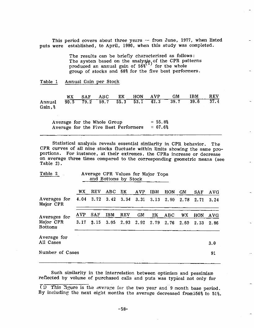
This period covers about three years - from June, 1977, when listed puts were established, to April, 1980, when this study was completed.

The results can be briefly characterized as follows: The svstem based on the analy&,of the CPR patterns produced an annual gain of 56%‘L’ for the whole group of stocks and 68% for the five best performers.

Table 1 Annual Gain per Stock

wx SAF ABC EK HON AVP GM IBM REV Annual 90.5 79.2 59.7 55.3 53.1 42.3 39.7 39.6 37.4 Gain,%

Average for the Whole Group = 55.8?j Average for the Five Best Performers = 67.6%

Statistical analysis reveals essential similarity in CPR behavior. The CPR curves of all nine stocks fluctuate within limits showing the same pro- portions. For instance, at their extremes, the CPRs increase or decrease on average three times compared to the corresponding geometric means (see Table 2).

Table 2 Average CPR Values for Major Tops and Bottoms by Stock

WX REV ABC EK AVP IBM HON GM SAF AVG

Averages for 4.04 3.72 3.42 3.34 3.31 3.13 2.90 2.78 2.71 3.24 Major CPR

Averages for AVP SAF IBM REV GM EK ABC WX HON AVG

Major CPR 3.17 3.15 3.05 2.93 2.92 2.79 2.76 2.60 2.33 2.86 Bottoms

Average for All Cases 3.8

Number of Cases 91

Such similarity in the interrelation between optimism and pessimism reflected by volume of purchased calls and puts was typical not only for

Ti, This ?igure is the averaie for the two year and ‘9 month base period. By including the next eight months the average decreased from556% to 51%.

-

-

-58-

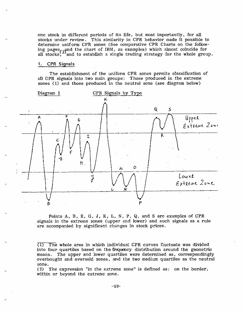
one stock in different periods of its life, but most importantly, for all stocks under review. This similarity in CPR behavior made it possible to determine uniform CPR zones (See comparative CPR Charts on the follow-

2: sy33 2Y d the chart of IBM, as examples) which almost coincide for

, and to establish a single trading strategy for the whole group.

1. CPR Signals

The establishment of the uniform CPR zones permits classification of all CPR signals into two main groups: Those produced in the extreme zones (1) and those produced in the neutral zone (see diagram below)

Diagram 1 CPR Signals by Type

K

Points A, B, E, G, J, K, L, N, P, Q, and S are examples of CPR signals in the extreme zones (upper and lower) and such signals as a rule are accompanied by significant changes in stock prices.

(1) The whole area in which individual CPR curves fluctuate was divided into four quartiles based on the f&quency distribution around the geometric means. The upper and lower quartiles were determined as, correspondingly overbought and oversold zones, and the two medium quartiles as the neutral zone. (2) The expression “in the extreme zone” is defined as: on the border, within or beyond the extreme zone.

-59-

~- .-.-- --

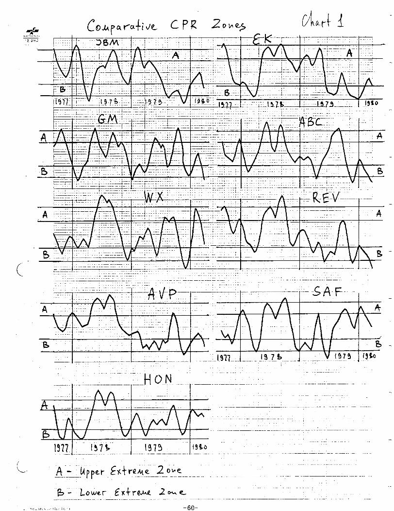
: c.

V

yFAp-.- --A.- -- .-- 1. __.__._ 1.97-l.. _.I ._... . !.3.7 .-

g-- --L-., -.-.. .--. v 1979-j _ : --.

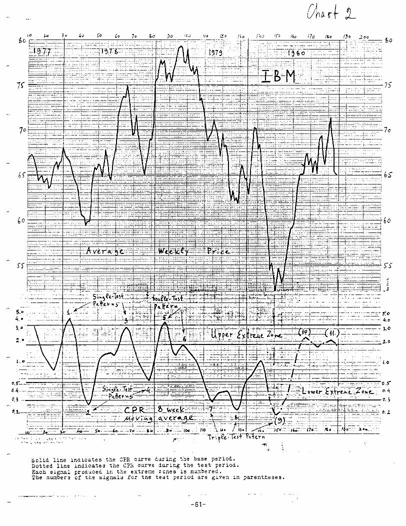
.O

0

*

------r---- -...-_.- ._- OS

.4

.3

Solid line indicates the CFR curve during the base period. Dotted line indicates the CPR curve during the test period. Each signal produced in the extreme zones is numbered. The numbers of tne signals for the test perrod are given in parentheses.

. - - - - - - . - I - . . - - - - ~ - . - - - .

-61-

The averagely ercentage gain for this category for the period under study was 8.06% . The extreme signals represent the majority of all signals (77 of 127, or 60.5%).

Points C, D, F, H, and I illustrate CPR signals in the neutral zone. There were 38 such signals, or 29.9%. The average percentage gain for sich a signal is much lower: 1.60%.

Points M, 0, and R represent trend resumption signals. Produced also in the extreme zones these signals signify the beginning of the repeated test of the top or the bottom.

The CPR curve, after such a signal, resumes the previous trend indicating that it has not yet ended.

The efficiency of such signals is very small. The average gain for 12 signals of this type was 0.66% per signal.

As the extreme signals are the strongest and the most interesting for trading practices, some of their other characteristics should be examined.

Table 3, following, shows that there is no sufficient difference between upward and downward extreme signals (8.66% and 7.44% per signal, correspondingly). There is also no serious difference between the signals produced on the border, within or beyond the extreme zones. The corresponding figures are 7.44%, 7.67% and 8.78%, “beyond” signals being slightly higher.

These figures show that the extreme signals of all types have almost equal potential to produce an average gain between 7 and 9% per case, and all of them can be used in trading practice.

The important data are represented in Table 4 on the following page. They show the distribution of the extreme signals with positive and negative return. Of 77 signals, 54 (or 70.1%) produced gains and 23 (or 29.9%) produced losses.

However, the average gain per positive signal is much higher than the average loss per negative one (+13.26% and -4.17% correspondingly). As a result all 77 signals gave an average gain of 8.06% per signal, which corresponds to 36% annual gain on a compound basis.

(1) The return on a CPR signal is calculated as percentage difference of stock price between two consecutive CPR signals regardless of their loca- tion .

-62-

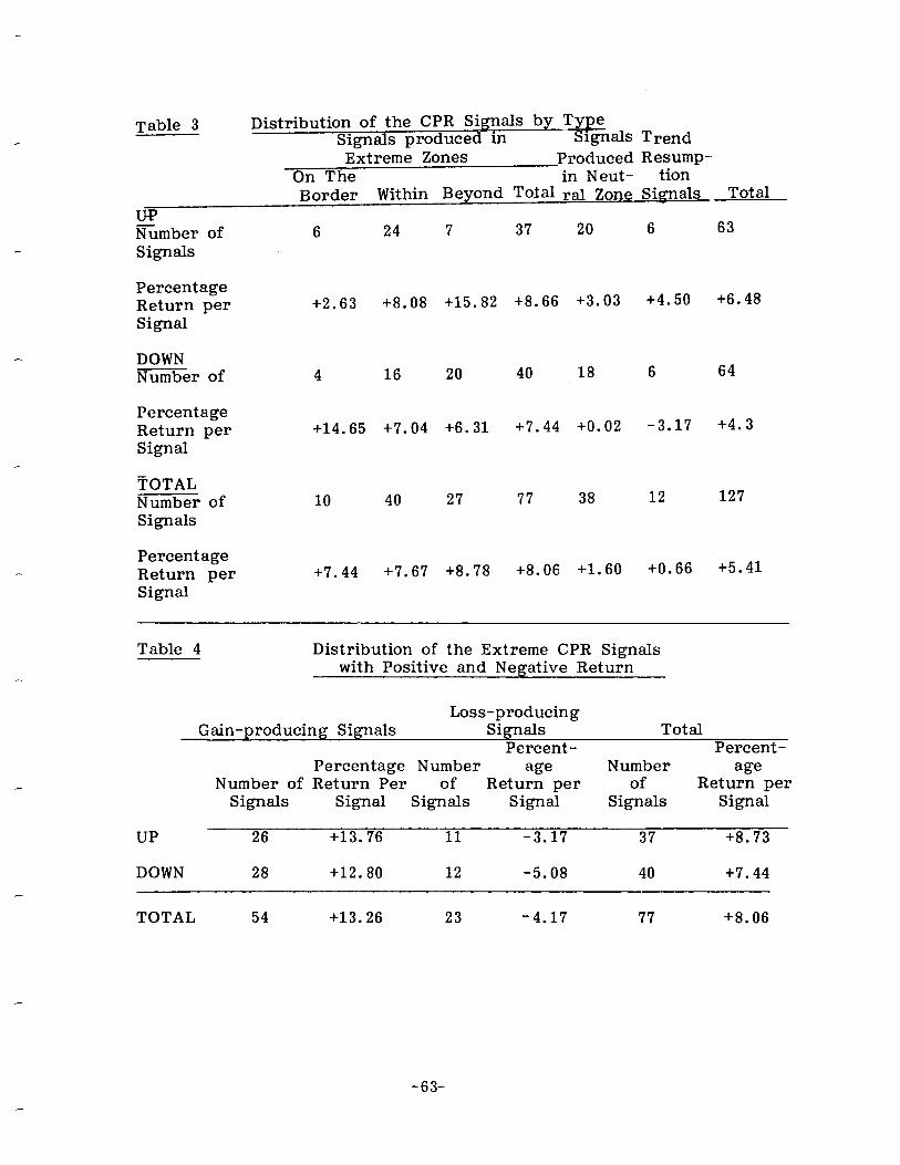
Table 3

VP Number of Signals

Distribution of the CPR Signals by Type Signals produced in Slgnahs Trend Extreme Zones Produced Resump-

On The in Neut- tion Border Within Beyond Total ral Zone Signals Total

6 24 7 37 20 6 63

Percentage Return per Signal

+2.63 +8.08 +15.82 +8.66 +3.03 +4.50 +6.48

DOWN Number of 4


+14.65

TOTAL Number of Signals

10


+7.44

16 20 40 18

+7.04 +6.31 +7.44 +o. 02

40 27 77 38

+7.67 +8.78 +8.06 +l. 60

6 64

-3.17

12

+0.66

+4.3

127

+5.41

Table 4 Distribution of the Extreme CPR Signals with Positive and Negative Return

Gain-producing Signals Loss-producing

Signals Percent-

Total Percent -

Percentage Number age Number age Number of Return Per of Return per of Return per

Signals Signal Signals Signal Signals Signal

26 +13.76 11 -3.17 37 +8.73

DOWN 28 +12.80 12 -5.08 40 +7.44

TOTAL 54 +13.26 23 -4.17 77 +8.06

-63-

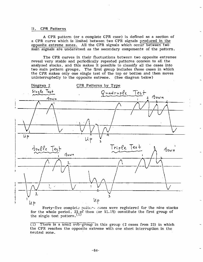
II. CPR Patterns

A CPR pattern (or a complete CPR case) is defined as a section of a CPR curve which is limited between two CPR signals produced in the opposite extreme zones. All the CPR signals which occur between two main signals are understood as the secondary components of the pattern.

The CPR curves in their fluctuations between two opposite extremes reveal very stable and periodically repeated patterns common to all the analyzed stocks, and this makes it possible to classify all the cases into two main pattern groups. The first group includes those cases in which the CPR makes only one single test of the top or bottom and then moves uninterruptedly to the opposite extreme. (See diagram below)

Diagram 2 CPR Patterns by Type

Forty-five complet? patter:, c;ises were registered for the nine stocks for the whole period, 2

Pe 1 f them (or 51.1%) constitute the first group of

the single test pattern.

(1) There is a small sub-group in this group (2 cases from 23) in which the CPR reaches the opposite extreme with one short interruption in the neutral zone.

-

-64-

The second group includes those cases in which the CPR makes several repeated tests of the top or bottom and moves to the opposite extreme only after having completed a series of such tests,. There are three sub-groups in this group: with two, three, and four consecutive tests of the extreme zones. (See Diagram 2).

In the second group the double-test sub-group is the largest one (15 cases out of 22). There were four cases with triple, and three cases with quadruple tests of the extreme zones.

The effectiveness of CPR signals which are regarded as a part of the pattern was measured in a different way than the effectiveness of CPR signlas as such. The following procedure was established :

1. The opening transactions are to be made only if the CPR produces a signal in the extreme zone.

2. If the CPR makes some repeated tests of the extreme zone, the opening transactions should be repeated as many times as such tests occur.

3. The closing transactions are to be made only when the CPR reaches the opposite extreme zone and produces a reversal signal. If several opening transactions were previously made, all of them should be closed simultaneously on such a reversal signal. The closing transactions should not be made on the CPR reversal signals in the neutral zone, nor on the CPR trend resumption signals.

The results of the CPR pattern effectiveness are represented in the following tables.

Table 5 shows the percentage return for the 9 stocks by signal and by pattern.

The application of the CPR patterns raised the average percentage gain per signal from 8.06 to 13.39%, or about 1.7 times. The upward signals were sufficiently higher than the downward signals (15.16% and 11.76% correspondingly).

The comparison of the pattern effectiveness shows that the most powerful was the single test group with the CPR moving uninterruptedly from one extreme to the opposite. The average percentage gain per pattern-case was 17.17%.

For the repeated test group the gains range as follows: 12.43% for the double-test pattern, 14.55% for the triple, and 7.37% for the quadruple test patterns with the average of 11.78% for the whole repeated test group.

Application of the CPR patterns significantly improves the ratio between positive and negative operations. The data are shown in Table 6.

-65-

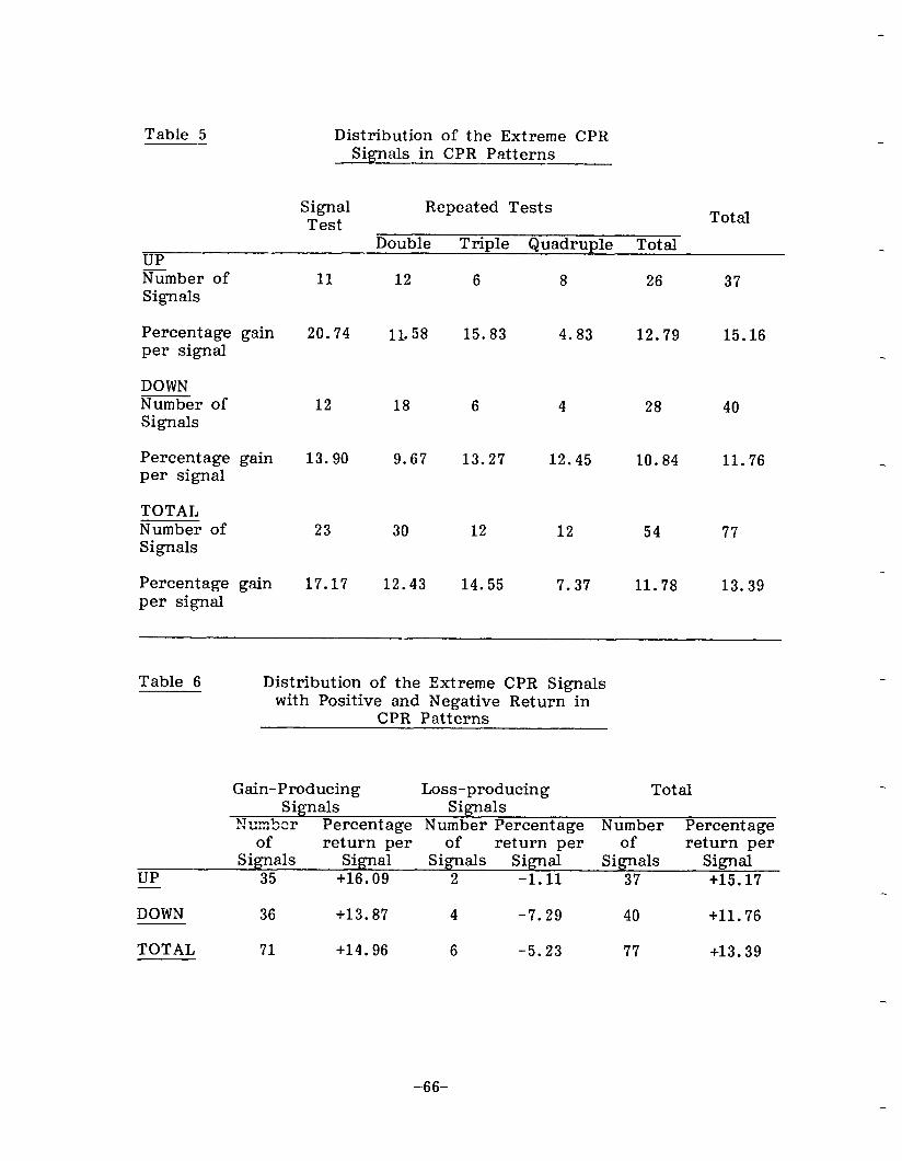
Table 5 Distribution of the Extreme CPR Signals in CPR Patterns

Signal Test

Repeated Tests Total

Double Triple Quadruple Total UP Number of 11 12 6 8 26 37 Signals

Percentage gain 20.74 11.58 15.83 4.83 12.79 15.16 per signal

DOWN Number of Signals

12 18 6 4 28 40

Percentage gain 13.90 9.67 13.27 12.45 per signal

10.84 11.76

TOTAL Number of 23 30 12 12 54 77 Signals

Percentage gain 17.17 12.43 14.55 7.37 11.78 13.39 per signal

Table 6 Distribution of the Extreme CPR Signals with Positive and Negative Return in

CPR Patterns

Gain-Producing Loss-producing Total Signals Signals

??umb2r Percentage Number Percentage Number Percentage of

Signals 35

return per of Signal

+16.09

return per of return per Signals Signal Signals Signal

2 -1.11 37 +15.17 UP

DOWN 36 +13.87 4 -7.29 40 +ll. 76

TOTAL 71 +14.96 6 -5.23 77 +13.39

-66-

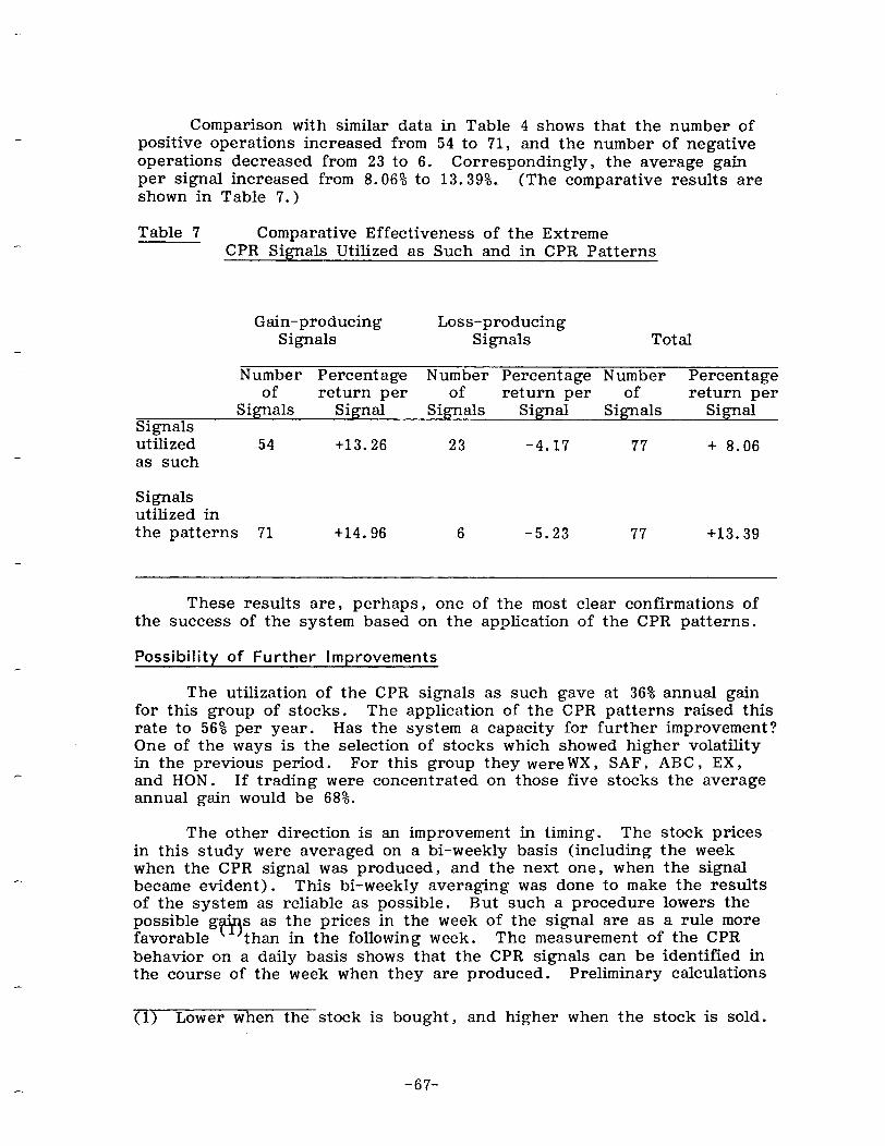
Comparison with similar data in Table 4 shows that the number of positive operations increased from 54 to 71, and the number of negative operations decreased from 23 to 6. Correspondingly, the average gain per signal increased from 8.06% to 13.39%. (The comparative results are shown in Table 7.)

Table 7 Comparative Effectiveness of the Extreme CPR Signals Utilized as Such and in CPR Patterns

Gain-producing Loss-producing Signals Signals Total

Signals utilized as such

Number Percentage Number Percentage Number Percentage of return per of return per of return per

Signals Signal Signals Signal Signals Signal

54 +13.26 23 -4.17 77 + 8.06

Signals utilized in the patterns 71 +14.96 6 -5.23 77 +13.39

These results are, perhaps, one of the most clear confirmations of the success of the system based on the application of the CPR patterns.

Possibility of Further Improvements

The utilization of the CPR signals as such gave at 36% annual gain for this group of stocks. The application of the CPR patterns raised this rate to 56% per year. Has the system a capacity for further improvement? One of the ways is the selection of stocks which showed higher volatility in the previous period. For this group they were WX, SAF, ABC, EX, and HON. If trading were concentrated on those five stocks the average annual gain would be 68%.

The other direction is an improvement in timing. The stock prices in this study were averaged on a bi-weekly basis (including the week when the CPR signal was produced, and the next one, when the signal became evident). This bi-weekly averaging was done to make the results of the system as reliable as possible. But such a procedure lowers the possible g@ s as the prices in the week of the signal are as a rule more favorable than in the following week. The measurement of the CPR behavior on a daily basis shows that the CPR signals can be identified in the course of the week when they are produced. Preliminary calculations

(1) Lower when the stock is bought, and higher when the stock is sold.

-67-

show that this improvement in timing can raise the average annual gain about 10%.

Analysis of the CPR behavior suggests some other ways of improvement . One of the findings of this study shows that the most powerful signals were those produced beyond the extreme zones (especially upward beyond signals which correspond to extremely oversold situations). On average the upward beyond signals (15.82%) are about two times stronger than all the extreme signals (8.06%). One of the possible strategies would indiate doubling investments on such signals.

All the above said shows that the system has a number of possibili- ties for further improvement, and that a model with 80% to 100% annual gain can be finally developed.

More Effective Utilization of the Repeated CPR Signals

It was indicated above that of the total 99 signals for 3.5 years only 9 caused losses and 90 produced gains. Table 8 shows the distribution of the positive and negative CPR signals according to their order of appearance.

Table 8

Single test pattern

Distribution of Positive and Negative CPR Signals in CPR Patterns

Repeated Signals All r-* A-L

First Second Third Fourth Repated All Signal Signal Signal Signal Signals Signals

28

Double test pattern 19

Triple test pattern 7

Quadruple test pattern 3

Total 57

Negative transactions 9

Positive transactions 48 29 10 3 42 90

19

7

3

29

--

-68-

7

3

10

--

3

3 42 99

-- -- 9

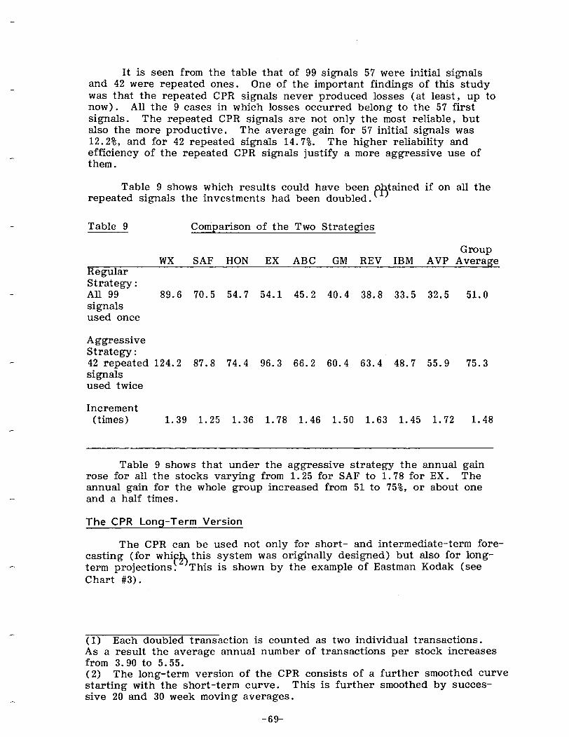
It is seen from the table that of 99 signals 57 were initial signals and 42 were repeated ones. One of the important findings of this study was that the repeated CPR signals never produced losses (at least, up to now). All the 9 cases in which losses occurred belong to the 57 first signals. The repeated CPR signals are not only the most reliable, but also the more productive. The average gain for 57 initial signals was 12.2%, and for 42 repeated signals 14.7%. The higher reliability and efficiency of the repeated CPR signals justify a more aggressive use of them.

Table 9 shows which results could have been repeated signals the investments had been doubled.

rbtained if on all the

Table 9 Comparison of the Two Strategies

Group wx SAF HON EX ABC GM REV IBM AVP Average

Regular Strategy : All 99 89.6 70.5 54.7 54.1 45.2 40.4 38.8 33.5 32.5 51.0 signals used once

Aggressive Strategy : 42 repeated 124.2 87.8 74.4 96.3 66.2 60.4 63.4 48.7 55.9 75.3 signals used twice

Increment (times) 1.39 1.25 1.36 1.78 1.46 1.50 1.63 1.45 1.72 1.48

Table 9 shows that under the aggressive strategy the annual gain rose for all the stocks varying from 1.25 for SAF to 1.78 for EX. The annual gain for the whole group increased from 51 to 75%, or about one and a half times.

The CPR Long-Term Version

The CPR can be used not only for short- and intermediate-term forecasting (for whi & this system was originally designed) but also for long- term projections. This is shown by the example of Eastman Kodak (see Chart #3).

(1) Each doubled transaction is counted as two individual transactions. As a result the average annual number of transactions per stock increases from 3.90 to 5.55. (2) The long-term version of the CPR consists of a further smoothed curve starting with the short-term curve. This is further smoothed by succes- sive 20 and 30 week moving averages.

-69-

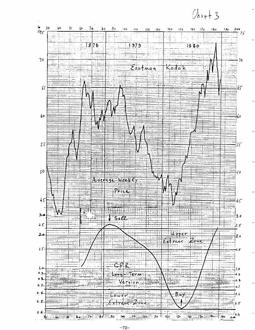
70

60

-7o-

The price ran through the whole cycle (from bottom to bottom) in two years. It formed a major bottom in April, 1978, finished forming a major top in the beginning of 1979 and again formed a major bottom in April, 1980.

Unfortunately, all of this becomes evident only in retrospect, as is always true as far as the stock prices is concerned. The basic character- istic of the CPR long-term version consists in its ability to determine the major stock trend in time not reacting to the intermediate price fluctuations. As seen from the charts, the CPR moves uninterruptedly from one extreme to the opposite and at its turning points it signals that the major trend has ended. Thus, the long-term CPR produces signals only when the stock forms a major top or bottom.

The Eastman Kodak Double Top lasted 2’7 weeks (weeks 62-99). The CPR produced its downward signal in advance (week 87). The stock moved down for almost the whole year, from 67 to 43. Subsequently, a major bottom was formed, and the CPR precisely identified it. During the next months EK rose from 43 to 75.

Table 10 summarizes the results.

Long-term CPR can be used in combination with the short-term CPR. Such a combination can provide better timing. In the case of Eastman Kodak, its short-term fourth downard signal (No. 7, week 99) which exactly coincided with the second tip could be used instead of the long-term signal or additionally to it because the long-term signal preceded it.

Table 10 Percentage Return on the Long-Term CPR Signals - Eastman Kodak

Opening Transactions Closing Transactions

Number Average Average Gain Duration of bi- bi- per in

Opera- Week weekly Week weekly signal Weeks tions No. Signal price No. Signal price (%)

1 87-88 Sell 61.00 152-153 Cover 51.38 18.72 66

2 152-153 BUY 51.38 181-182* Sell 71.69 39.53 30

Average for EX *Preliminary

29.13 48.0

The CPR does not indicate the extent of price movement. It only shows the reverse points. As far as EK is concerned, its long-term CPR entered in November, 1980 a critical area, indicating that the basic growth potential of this stock was exhausted.

-71-

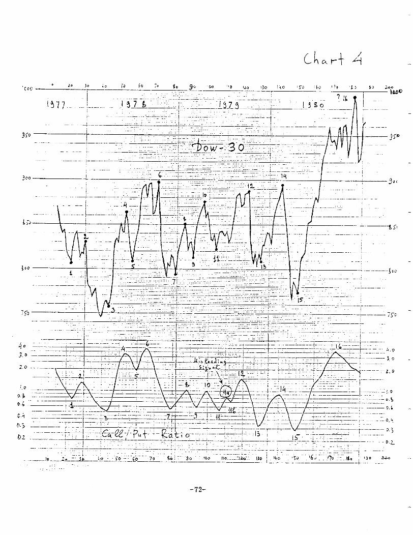
‘IO ILrJ I30 Ii0 ‘r3 :bo ‘?O ‘I>

-.:-: .-.I -. ‘-13 : ! ! L--p- I I. h

-72-

Not all stocks run through such well-defined long-term cycles as did EK, but when such a cycle occurs the CPR reveals it precisely, and identifies the major top and bottom areas in time. The data for two stocks is, of course, not sufficient to draw final conclusions, but it can be expected that the study of a large number of cases will prove that the CPR may be an extremely valuable tool for long-term forecasting.

Call/Put Ratio for General Timing

The CaIl/Put Ratio can be successfully used to forecast turning points of the stock market as a whole.

Chart #4 shows the behavior of the aggregate CPR for the nine analyzed stocks. From the Chart it is seen that during 3.5 years of 15 instances when the stock market changed its direction the CPR produced only one misleading signal (week 111, signal No. 11-a). In all the remain- ing instances the CPR either correctly predicted or confirmed in time the corresponding market movements.

Table 11 shows the CPR lead time in weeks. For significant market movements as a rule CPR produced signals in advance or exactly on time (the average = -1.13 weeks). For less serious movements CPR signals are slightly delayed (the average = +1. 00) . For all 15 cases the average = -0.13. Thus, the CPR on the average produces its signals on time.

From the above figures the following conclusions may be formulated:

1. If the CPR produces a delayed signal the corresponding market movement will not be serious.

2. If the CPR produces an advanced signal the corresponding market movement will be at least 100 points.

Concerning the last case (No. 16) it is too early to draw any final conclusion. Most likely this signal predicts very serious market decline, probably, the beginning of a bear market. As far as the 15 completed cases are concerned, the ratio of correct to incorrect signals is expressed by the proportion 14 : 1.

-73-

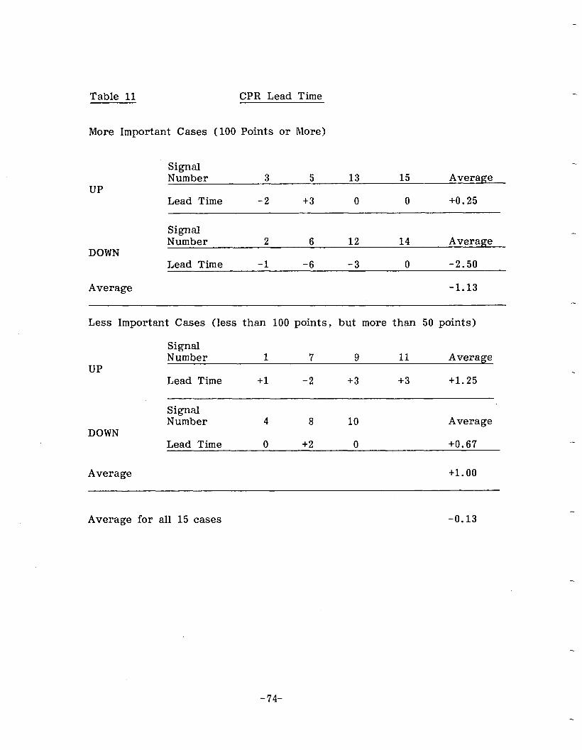
Table 11 CPR Lead Time

More Important Cases (100 Points or More)

UP

Signal Number

Lead Time

3 5 13

-2 +3 0

15 Average

0 +0.25

SignaI Number 2 6 12 14 Average

DOWN Lead Time -1 -6 -3 0 -2.50

Average -1.13

Less Important Cases (less than 100 points, but more than 50 points)

UP

Signal Number 1 7 9 11 Average

Lead Time +l -2 +3 +3 +1.25

DOWN

Signal Number 4 8 10 Average

Lead Time 0 +2 0 +0.67

Average +1.00

Average for all 15 cases -0.13

-74-

journal of technical analysis (jota). issue 14 (1982, august)

Economy & Finance