journal of sound and vibration - acoustics and dynamics ... and...stiffness matrix formulation for...

Contents lists available at SciVerse ScienceDirect

Journal of Sound and Vibration

Journal of Sound and Vibration 332 (2013) 5898–5916

0022-46http://d

n CorrE-m

journal homepage: www.elsevier.com/locate/jsvi

Stiffness matrix formulation for double row angular contactball bearings: Analytical development and validation

Aydin Gunduz, Rajendra Singh n

Acoustics and Dynamics Laboratory, Department of Mechanical & Aerospace Engineering and Smart Vehicles Concepts Center,The Ohio State University, Columbus, Ohio 43210, USA

a r t i c l e i n f o

Article history:Received 10 July 2012Received in revised form12 March 2013Accepted 6 April 2013
Handling Editor: H. Ouyang
literature, a new, comprehensive, analytical approach is proposed based on the Hertzian

Available online 13 July 2013

0X/$ - see front matter & 2013 Elsevier Ltd.x.doi.org/10.1016/j.jsv.2013.04.049

esponding author. Tel.: +1 614292 9044; faxail address: [email protected] (R. Singh).

a b s t r a c t

Though double row angular contact ball bearings are widely used in industrial, automotive,and aircraft applications, the scientific literature on double row bearings is sparse. It is alsoshown that the stiffness matrices of two single row bearings may not be simply superposedto obtain the stiffness matrix of a double row bearing. To overcome the deficiency in the

theory for back-to-back, face-to-face, and tandem arrangements. The elements of the five-dimensional stiffness matrix for double row angular contact ball bearings are computedgiven either the mean bearing displacement or the mean load vector. The diagonal elementsof the proposed stiffness matrix are verified with a commercial code for all arrangementsunder three loading scenarios. Some changes in stiffness coefficients are investigated byvarying critical kinematic and geometric parameters to provide more insight. Finally, thecalculated natural frequencies of a shaft-bearing experiment are successfully comparedwith measurements, thus validating the proposed stiffness formulation. For double rowangular contact ball bearings, the moment stiffness and cross-coupling stiffness terms aresignificant, and the contact angle changes under loads. The proposed formulation is alsovalid for paired (duplex) bearings which behave as an integrated double row unit when thesurrounding structural elements are sufficiently rigid.

& 2013 Elsevier Ltd. All rights reserved.

1. Introduction

Double row bearings offer certain advantages over single row bearings, as they are capable of providing higher axial andradial rigidity and carrying bi-directional or combined loads. Consequently, double row bearings are widely used in machinetool spindles, industrial pumps, and air compressors, as well as in automotive, helicopter, and aircraft applications such asgear boxes, wheel hubs, and helicopter rotors [1–3]. In certain problems, a double row bearing may be simply representedby two single row bearings attached next to each other. However, in many static and dynamic problems, a double rowbearing must be considered as an integrated unit. The stiffness matrices of two single row bearings may not be simplysuperposed to obtain the stiffness matrix of a double row bearing.

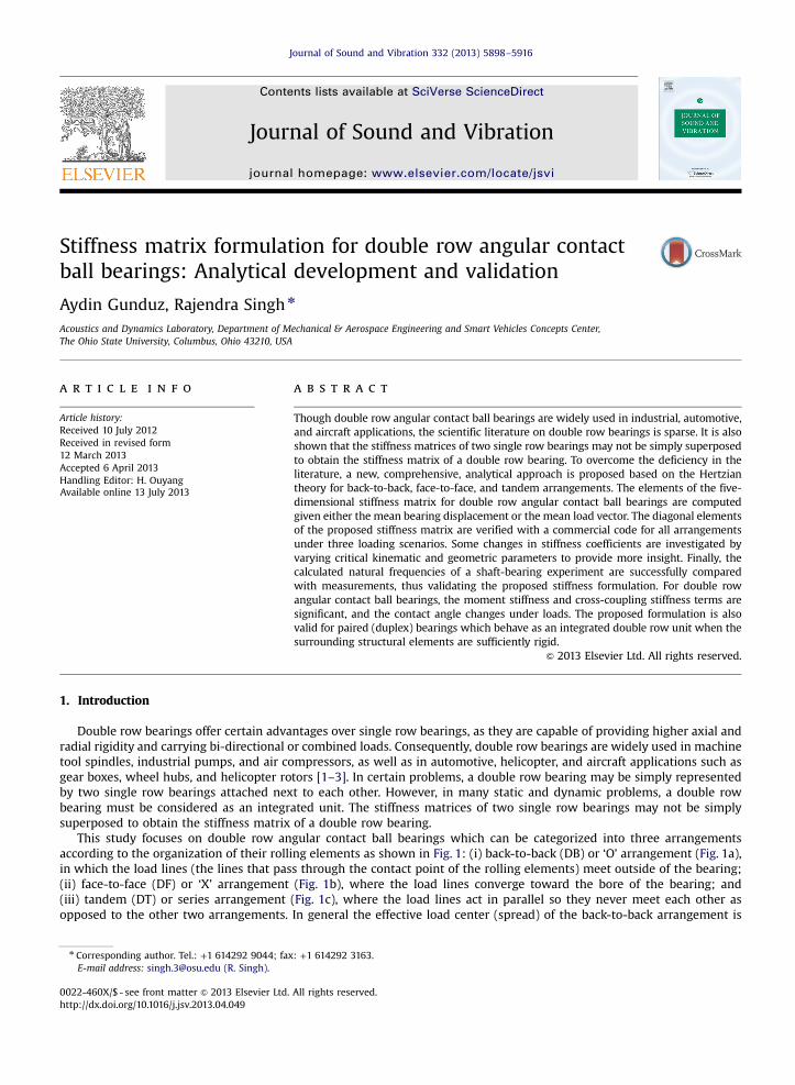
This study focuses on double row angular contact ball bearings which can be categorized into three arrangementsaccording to the organization of their rolling elements as shown in Fig. 1: (i) back-to-back (DB) or ‘O’ arrangement (Fig. 1a),in which the load lines (the lines that pass through the contact point of the rolling elements) meet outside of the bearing;(ii) face-to-face (DF) or ‘X’ arrangement (Fig. 1b), where the load lines converge toward the bore of the bearing; and(iii) tandem (DT) or series arrangement (Fig. 1c), where the load lines act in parallel so they never meet each other asopposed to the other two arrangements. In general the effective load center (spread) of the back-to-back arrangement is

All rights reserved.

: +1 614292 3163.

www.sciencedirect.com/science/journal/0022460X

www.elsevier.com/locate/jsvi

http://dx.doi.org/10.1016/j.jsv.2013.04.049



http://crossmark.dyndns.org/dialog/?doi=10.1016/j.jsv.2013.04.049&domain=pdf



mailto:[email protected]


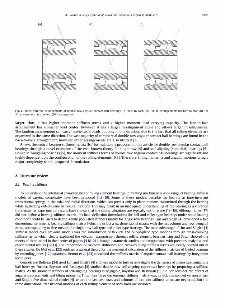
Fig. 1. Three different arrangements of double row angular contact ball bearings: (a) back-to-back (DB) or ‘O’ arrangement; (b) face-to-face (DF) or‘X’ arrangement; (c) tandem (DT) arrangement.

A. Gunduz, R. Singh / Journal of Sound and Vibration 332 (2013) 5898–5916 5899

larger; thus, it has higher moment stiffness terms and a higher moment load carrying capacity. The face-to-facearrangement has a smaller load center; however, it has a larger misalignment angle and allows larger misalignments.The tandem arrangement can carry heavier axial loads but only in one direction due to the fact that all rolling elements areorganized in the same direction. The vast majority of commercial double row angular contact ball bearings are found in theback-to-back arrangement; however, other arrangements are also utilized [1].

A new, theoretical bearing stiffness matrix (Kb) formulation is proposed in this article for double row angular contact ballbearings through a novel extension of the well-known theory for single row [4] and self-aligning (spherical) bearings [5].Unlike self-aligning bearings [5], the moment stiffness terms of double row angular contact ball bearings are significant andhighly dependent on the configuration of the rolling elements [6,7]. Therefore, tilting moments and angular motions bring amajor complexity to the proposed formulation.

2. Literature review

2.1. Bearing stiffness

To understand the interfacial characteristics of rolling element bearings in rotating machinery, a wide range of bearing stiffnessmodels of varying complexity have been proposed [1,8–16]. Some of these models describe the bearing as time-invarianttranslational springs in the axial and radial directions, which can predict only in-plane motions transmitted through the bearingwhile neglecting out-of-plane or flexural motions. This may result in an inadequate understanding of the bearing as a vibrationtransmitter, as experimental results have shown that the casing vibrations are typically out-of-plane [13–15]. Although Jones [17]did not define a bearing stiffness matrix, his load–deflection formulations for ball and roller type bearings under static loadingconditions could be used to define a fully populated stiffness matrix for single row bearings. Lim and Singh [4] developed a fivedimensional symmetric bearing stiffness matrix (which is in fact a six dimensional matrix with the last column and row being allzeros, corresponding to free torsion) for single row ball-type and roller-type bearings. The main advantage of Lim and Singh's [4]stiffness model over previous models was the introduction of flexural and out-of-plane type motions through cross-couplingstiffness terms which clearly explained the vibration transmission through rolling element bearings. Lim and Singh showed themerits of their model in their series of papers [4,18–21] through parametric studies and comparisons with previous analytical andexperimental results [12,13]. The importance of moment stiffnesses and cross-coupling stiffness terms are clearly pointed out inthese studies. De Mul et al. [22] outlined a general theory for the numerical calculation of the stiffness matrices of loaded bearingsby extending Jones' [17] equations. Hernot et al. [23] calculated the stiffness matrix of angular contact ball bearings by integrationtechniques.

Cermelj and Boltezar [24] used Lim and Singh's [4] stiffness model to further investigate the dynamics of a structure containingball bearings. Further, Royston and Basdogan [5] studied double row self-aligning (spherical) bearings by proposing a stiffnessmatrix. As the moment stiffness of self-aligning bearings is negligible, Royston and Basdogan [5] did not consider the effects ofangular displacements and tilting moments. Thus, their three dimensional stiffness matrix was, in fact, a simplified version of Limand Singh's five dimensional model [4], where the last two rows and columns of moment stiffness terms are neglected, but thethree dimensional translational motions of each rolling element of both rows are included.

A. Gunduz, R. Singh / Journal of Sound and Vibration 332 (2013) 5898–59165900

Guo and Parker [25] have recently proposed a numerical method for calculating the bearing stiffness matrix of single-row bearings with a commercial finite element based contact mechanics code [26]. Their numerical approach, however,is not attractive since at least 50 executions of the finite element code (hence excessive computing times) are needed toestimate Kb; and also, utilization of finite difference approximation [25] may create problems. Additionally it is not clear ifthe double row bearings can be analyzed with this method. Thus, analytical methods must be preferred over such numericalmethods for the theoretical calculation of Kb as well as insight into the significance of various terms.

Experimental techniques have also been utilized to measure radial and axial bearing stiffness coefficients. For example, Walfordand Stone [27,28] used a two-degree-of-freedom model to extract representative stiffness values from measurements. Stone [29]reviewed various efforts to measure the stiffness and damping coefficients of rolling element bearings with changes in preload,speed, or lubrication. Kraus et al. [13] designed an in-situ measurement test to determine the translational bearing stiffnessmeasured from vibration spectra using a single-degree-of-freedom model. Marsh and Yantek [30] extracted translational bearingstiffness coefficients by measuring the resulting responses under known excitation forces. Tiwari and Vyas [31] suggested a methodfor estimating nonlinear bearing parameters without making explicit force measurements. Finally, Pinte et al. [32] experimentallyminimized coupling between horizontal and vertical directions by using hinges and leaf springs in order to block out-of-planeforces when they developed a piezo-based bearing for active noise control.

2.2. Double row bearings

Although single row bearings have been extensively studied, publications specific to double row bearings are sparse. Forinstance, Bercea et al. [6] formulated the relative displacement between the bearing rings (also termed as the ‘ringapproach’) for various double row bearing types such as tapered, spherical, cylindrical roller, and angular contact ballbearings. Their bearing deflection formulation is only valid for a back-to-back arrangement and did not include any stiffnessformulation. Then Nelias and Bercea [7] used their double row tapered rolling bearing model for case studies. Cao and Xiao[33] developed a dynamic model for double row spherical roller bearings based on energy principles. Later Cao [34]improved this model by including the effects of rotational motions and shaft misalignments. Choi and Yoon [35] proposeda method for determining discrete design variables of an automotive wheel assembly that contained a double row angularcontact ball bearing. Their optimization algorithm attempted to maximize the bearing service life while satisfying variousdesign constraints including limited mounting space.

3. Stiffness formulations of a double row bearing vs. two single row bearings

Two approaches may be utilized in the stiffness modeling of double row or duplex angular contact ball bearings asshown in Fig. 2(a–b). The first approach (with two single row bearings) essentially yields 2 separate mean displacementqim ¼ fδixm; δiym; δizm; βixm; βiymgT and load vectors fim ¼ fFixm; Fiym; Fizm;Mi

xm;MiymgT (here z-axis is the rotational axis) and two

separate stiffness (Kib) matrices (i.e. one for each individual bearing) where

Kib ¼

kixx kixy kixz kixθx kixθy

kiyx kiyy kiyz kiyθx kiyθy

kizx kizy kizz kizθx kizθy

kiθxx kiθxy kiθxz kiθxθx kiθxθy

kiθyx kiθyy kiθyz kiθyθx kiθyθy

266666666664

377777777775

ði¼ 1;2Þ (1)

Conversely, the second approach results in single mean displacement qDm ¼ fδDxm; δDym; δDzm; βDxm; βDymgT and load fDm ¼ fFDxm;

FDym; FDzm;M

Dxm;M

DymgT vectors. Note that a single stiffness matrix (KD

b ) needs to be defined for the double row bearing where

K(2)

Translational stiffness elements of two side by side bearings with the same shaft and housing are in parallel [36]; thus,they can be superposed to obtain the stiffness values of the integrated unit (i.e. kDpq≈k

1pq þ k2pq where p,q¼x, y, z). However,

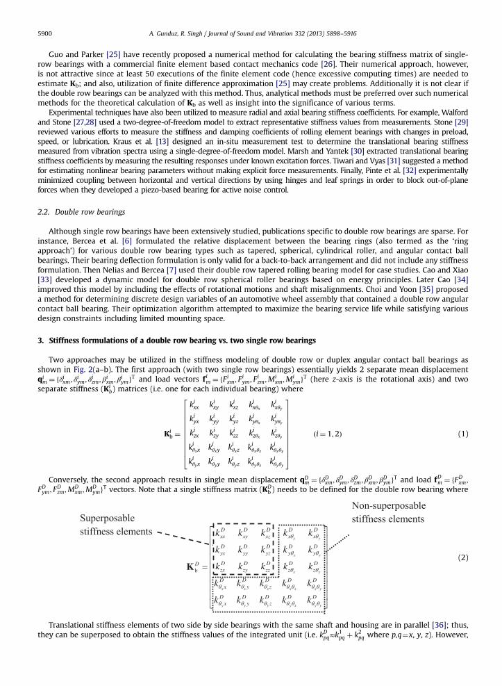
Table 1Kinematic properties of the example case: Double row angular contact ball bearing.

Symbol Value Description

Z 14 Number of rolling elements in one rowrL (mm) 0 Radial clearanceKn (N/mm1.5) 395,000 Hertzian stiffness constantR (mm) 34.75 Radius of the inner raceway groove curvature center (pitch radius)Ao (mm) 0.52 Unloaded distance between inner and outer raceway centerse (mm) 10.0 Axial distance between the geometric center and bearing one rowαo (deg) 30 Unloaded contact anglen 1.5 Load–deflection exponent

BRG2zBRG1z

1BRGz

Bearing 2

O

Inner ring

Outer ring Gz

Double row angular contact ball bearing

(DB, DF or DT configuration)

G

lSHAFT

x

zextzF

extxF

y

O

Bearing 1

Gz

G

lSHAFT

x

extzF

extxF

y

z

Fig. 2. Illustration of two approaches that can be practiced in modeling of double row/duplex angular contact ball bearings: (a) Modeling two single rowbearings, and (b) modeling an integrated double row bearing. Here, the rigid shaft is subjected to radial ðFextx Þ and axial ðFextz Þ external loads at point O.


the rotational stiffness or rotational coupling terms ðkrs where r or s¼ θx; θyÞ of two single row bearings and a double rowbearing may not be easily correlated. In fact, there is simply no way of obtaining kDrs from kirs (i¼1,2), as kDrs terms depend ongeometric parameters and the organization of rolling elements; thus, they must be derived from basic load–deflectionrelations.

To illustrate the above-mentioned issues, consider an illustrative example with a 148 mm long uniform solid shaft with adiameter of 50 mm as shown in Fig. 2(a–b). First, two single row bearings (in all three arrangements) are placed on the shaftwith z-coordinates zBRG1¼64 mm and zBRG2¼84 mm, respectively. These two bearings are then replaced with a double rowbearing with its geometric center located at zG¼74 mm (zG ¼ ðzBRG1 þ zBRG2Þ=2). The kinematic properties of the bearing aregiven in Table 1. The external load is applied at point O with magnitudes Fextx ¼ 1 kN and Fextz ¼ 3 kN. Observe that Fextximposes a bending moment (Mi

ym) on both bearings. A combined asymmetrical loading case ensures that the analysispresents a general case. The diagonal stiffness elements of the bearings (i.e. kpp where p¼x,y,z,θx; θy) are calculated using acommercial code [8]. This particular code [8] contains a large bearing library of commercial single and double row bearingsfrom major manufacturers, and yields only the diagonal elements of Kb which is sufficient and convenient for thecomparative analysis. The calculated elements of Kb under the combined load are listed in Table 2(a–c). It is clear from thetables that kDpp≈k

1pp þ k2pp is valid for p¼x,y,z but not for p¼ θx; θy for all arrangements. Note that the overall tilting

characteristics of a shaft-bearing system are dictated by kDθxθx and kDθyθy terms but not the kiθxθx and kiθyθy (i¼1, 2) termsindividually. Since it is not possible to obtain the rotational stiffness or rotational coupling terms of a double row bearing (kDrs

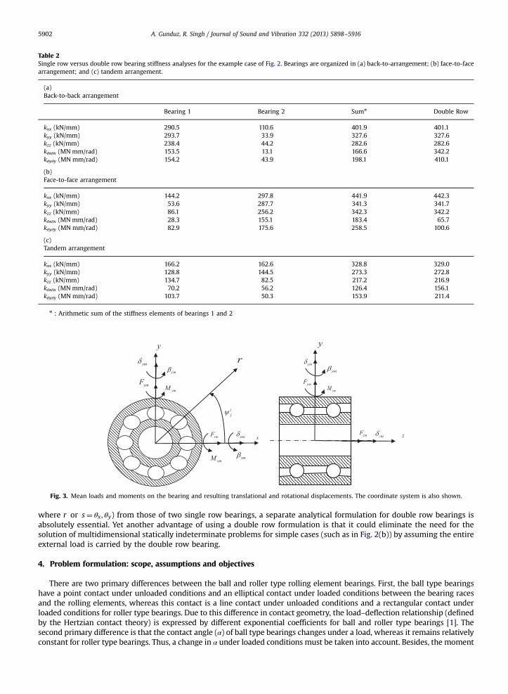
Fig. 3. Mean loads and moments on the bearing and resulting translational and rotational displacements. The coordinate system is also shown.

Table 2Single row versus double row bearing stiffness analyses for the example case of Fig. 2. Bearings are organized in (a) back-to-arrangement; (b) face-to-facearrangement; and (c) tandem arrangement.

(a)Back-to-back arrangement

Bearing 1 Bearing 2 Sumn Double Row

kxx (kN/mm) 290.5 110.6 401.9 401.1kyy (kN/mm) 293.7 33.9 327.6 327.6kzz (kN/mm) 238.4 44.2 282.6 282.6kθxθx (MN mm/rad) 153.5 13.1 166.6 342.2kθyθy (MN mm/rad) 154.2 43.9 198.1 410.1

(b)Face-to-face arrangement


(c)Tandem arrangement


n : Arithmetic sum of the stiffness elements of bearings 1 and 2


where r or s¼ θx; θy) from those of two single row bearings, a separate analytical formulation for double row bearings isabsolutely essential. Yet another advantage of using a double row formulation is that it could eliminate the need for thesolution of multidimensional statically indeterminate problems for simple cases (such as in Fig. 2(b)) by assuming the entireexternal load is carried by the double row bearing.

4. Problem formulation: scope, assumptions and objectives

There are two primary differences between the ball and roller type rolling element bearings. First, the ball type bearingshave a point contact under unloaded conditions and an elliptical contact under loaded conditions between the bearing racesand the rolling elements, whereas this contact is a line contact under unloaded conditions and a rectangular contact underloaded conditions for roller type bearings. Due to this difference in contact geometry, the load–deflection relationship (definedby the Hertzian contact theory) is expressed by different exponential coefficients for ball and roller type bearings [1]. Thesecond primary difference is that the contact angle (α) of ball type bearings changes under a load, whereas it remains relativelyconstant for roller type bearings. Thus, a change in α under loaded conditions must be taken into account. Besides, the moment


stiffnesses and the cross-coupling stiffness coefficients of the angular contact ball bearings are significant. Therefore, some ofthe simplifying assumptions made for some other bearing types do not hold for angular contact ball bearings.

For the sake of analytical development, consider the double row angular contact ball bearing with a mean bearing loadvector fm ¼ fFxm; Fym; Fzm;Mxm;MymgT and the resulting mean displacement vector qm ¼ fδxm; δym; δzm; βxm; βymgT, as illustratedin Fig. 3 (beyond this point, all symbols are relevant to a double row bearing, and thus the superscript ‘D’ is simply omittedfor the sake of convenience). Here δxm; δym; δzm and Fxm; Fym; Fzm are the mean displacements and loads in the x, y, and zdirections, and βxm, βymand Mxm, Mym are the mean angular displacements and tilting moments about the x and ycoordinates, respectively. The shaft is allowed to rotate freely about the z-axis so the corresponding angular displacementand torsional terms are zero.

In general, both the inner and outer rings of a rolling element bearing may deflect under a load. However, for the purposes ofthis study it is sufficient to consider only the relative displacement between the bearing rings. Thus, assuming the outer ring isfixed in space and the inner ring is displaced under a load permits a tractable approach which is also pointed out by previousinvestigators [4,22]. The mean bearing load vector (fm) will be considered as an effective point load on the inner ring and actingalong the geometrical center of the bearing. Similarly, the mean displacement vector qm corresponds to the displacement of thebearing center. The total displacement vector is defined as q(t)¼qm+qa(t), where qa(t) is the alternating displacement vector thatfluctuates about the mean point qm. For small mean loads or sufficiently high dynamic displacements, the bearing stiffnessis time-varying, and nonlinear models should be used for the dynamic analysis. In this analysis it is assumed that |qa(t)| is muchsmaller than qm; thus, linearized and time-invariant values of bearing stiffness can be determined about an operating point. Inthis study, it is assumed that both rows of the bearings are identical in terms of the structural and kinematic parameters. Sincethe bearings are often mounted on rigid shafts, and within robust housings the structural deformation of bearing rings isassumed to be negligible, and only the elastic deformation of the rolling elements at contact points is considered. It is assumedthat the elastic deformation of the rolling elements occurs according to the Hertzian contact stress theory [1], and the loadexperienced by each rolling element is defined by its angular position in the bearing raceway. The internal friction is alsoassumed to be negligible compared with the normal loads on rolling elements. Further, the angular position of each rollingelement relative to one another remains the same due to rigid cages and retainers. It is also assumed that the bearing does notoperate at overcritical speeds; therefore, the gyroscopic moments and centrifugal effects can be neglected. It is assumed that thelubrication does not directly affect the bearing stiffness coefficients except at very high speeds, as explained in the earlier work[4,5]; this assumption is also utilized in some commercial codes [8]. Thus, tribological issues are beyond the scope of this paper.Nevertheless, the authors have shown that the effect of lubrication can be successfully included via bearing (viscous) dampingelements in their recent work [36,37]. Finally the proposed Kb is also valid for duplex (paired) bearings mounted in face-to-face,back-to-back, or tandem arrangements, assuming all structural elements (such as the shaft and bearing rings) are sufficientlyrigid; thus, the inner rings of the two rows do not move independently under external loads (except initial preloading).

The specific objectives of this study can be listed as follows: (1) develop a systematic and comprehensive approach todetermine the fully populated five dimensional stiffness matrix (Kb) for double row angular contact ball bearings of back-to-back, face-to-face, and tandem arrangements (which may be extended for other types of double row bearings in laterstudies); (2) develop a numerical scheme to compute Kb given the mean displacement (qm) or the mean loading (fm)vectors; (3) verify the diagonal elements of the proposed stiffness matrix with a commercial code for all arrangements forvarious load cases; (4) conduct parametric studies to observe the effect of different loading scenarios, unloaded contactangle, and angular position of the bearing on the stiffness coefficients; and (5) validate the proposed model by comparingthe natural frequencies of a vehicle wheel bearing assembly with the measurements on a double row angular contact ballbearing (in the back-to-back arrangement).

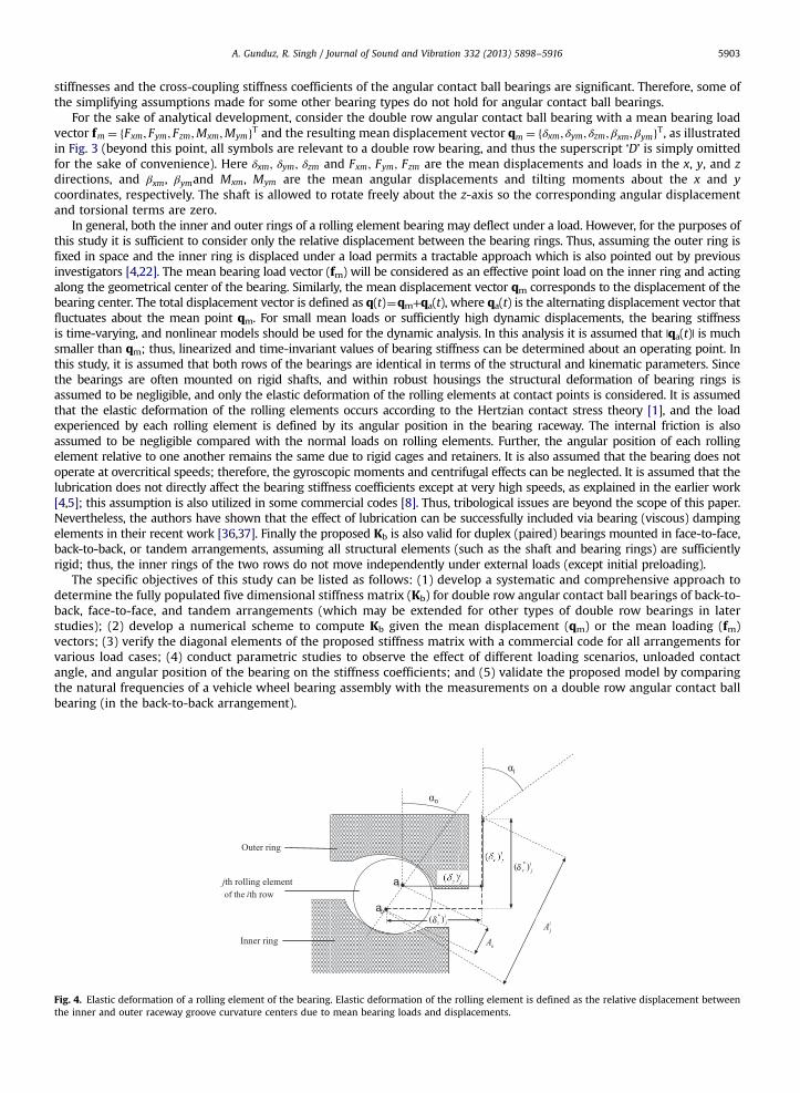
Fig. 4. Elastic deformation of a rolling element of the bearing. Elastic deformation of the rolling element is defined as the relative displacement betweenthe inner and outer raceway groove curvature centers due to mean bearing loads and displacements.


5. New analytical formulation: load–deflection relations of a rolling element

To define the bearing stiffness, the relationship between fm and qm will first be derived. Consider the jth rolling elementof the ith row of a double row angular contact ball bearing shown in Fig. 4. Assuming the outer ring is fixed, the total elasticdeformation δðψ i

jÞ of this rolling element can be calculated by

δðψ ijÞ ¼

Aij−Ao for δðψ i

jÞ40

0 for δðψ ijÞ≤0

8<: (3)

Here, ψ ij is the angular distance of the rolling element from the x-(horizontal) axis, and Ao and Ai

j are the unloaded andloaded relative distances between the inner and outer raceway groove curvature centers, respectively. If Ao is greater than Ai

j,the rolling element is unloaded, and the elastic deformation is zero. To calculate Ai

j, the radial and axial displacementsððδrÞij and ðδzÞijÞ of the rolling element are first expressed in terms of the elements of bearing displacement vector qm

ðδrÞij ¼ ½δxm þ c1βyme� cos ðψ ijÞ þ ½δym−c1βxme� sin ðψ i

jÞ−rL (4a)

ðδzÞij ¼ δzm þ R½βxm sin ðψ ijÞ−βym cos ðψ i

jÞ� (4b)

Here R is the radius of the inner raceway groove curvature center (pitch radius), αo is the unloaded contact angle, rL is theradial clearance, and e is the axial distance between the geometric center of the bearing and bearing rows. The effective loadcenter (E), which controls the tilting stiffness terms of a double row arrangement, can be defined as E¼ 2ðeþ c2R tan ðαoÞÞ,and coefficients c1 and c2 are given as follows:

c1 ¼−1 for i¼ 1 ðLeft rowÞ1 for i¼ 2 ðRight rowÞ

((5)

c2 ¼1 back� to� back ðDBÞ arrangement−1 face� to� face ðDFÞ arrangement0 tandem ðDTÞ arrangement

8><>: (6)

The net (effective) radial ðδnr Þij and axial ðδnz Þij displacements of the rolling element are then expressed including the effectsof initial displacement due to the unloaded contact angle αo

ðδnr Þij ¼ ðδrÞij þ Ao cos ðαoÞ (7a)

ðδnz Þij ¼ ðδzÞij þ c3ðAo sin ðαoÞ þ ðδz0ÞiÞ (7b)

Here ðδz0Þi defines an axial displacement preload on the ith row obtained by bringing the inner and outer raceways closertogether by a distance ðδz0Þi (for instance in the case of split inner rings [35]). ðδz0Þi can have a positive value only if the radialclearance is eliminated (i.e. rL ¼ 0). Here, c3 is a constant dependent on the type of rolling element bearing

Back� to� back ðDBÞ arrangement : c3 ¼1 for i ¼ 1 ðLeft rowÞ−1 for i ¼ 2 ðRight rowÞ

((8a)

Face� to� face ðDFÞ arrangement : c3 ¼−1 for i ¼ 1 ðLeft rowÞ1 for i ¼ 2 ðRight rowÞ

((8b)

Tandem ðDTÞ arrangement : c3 ¼ 1ðnÞ ðBoth rowsÞ (8c)

(*): Assuming the tandem arrangement is axially loaded in the direction it can hold.The loaded relative distance between the inner and outer raceway groove curvature center Aðψ i

jÞ is finally obtained byvectoral addition of the net displacements

Aðψ ijÞ ¼

ffiffiffiffiffiffiffiffiffiffiffiffiffiffiffiffiffiffiffiffiffiffiffiffiffiffiffiffiffiffiffiffiffiffiffiððδnr ÞijÞ2 þ ððδnz ÞijÞ2

q(9)

Then, the elastic deformation δðψ ijÞ of the rolling element can be determined by Eq. (3) to be used in conjunction with the

Hertzian contact stress theory in order to obtain the resultant normal load (Qij) on the element

Qij ¼ Knðδðψ i

jÞÞn: (10)

Here Kn is the rolling element load–deflection stiffness constant, which is a function of material properties and geometry [1].The exponent n is equal to 1.5 for point/elliptical type contact (for ball type bearings). The loaded contact angle αij for the


same element is determined by trigonometry

tan ðαijÞ ¼ðδnz Þijðδnr Þij

¼ ðδzÞij þ c3ðAo sin ðαoÞ þ ðδz0ÞiÞðδrÞij þ Ao cos ðαoÞ

(11)

where ðδzÞij and ðδrÞij are given by Eq. (4a and b).

6. Stiffness matrix

6.1. Formulation

The bearing stiffness matrix is a comprehensive representation that combines the bearing's kinematic and elasticproperties and the effect of each rolling element [4]. To apply the mathematical definition of the stiffness matrix, the meanload vector fm is first represented through vectoral sums of Qi

jði¼ 1;2; j¼ 1;…; ZÞ for each loaded ðδðψ ijÞ40Þ rolling element

as follows:

fm ¼

FxmFymFzmMxm

Mym

8>>>>>><>>>>>>:

9>>>>>>=>>>>>>;

¼ ∑2

i ¼ 1∑Z

j ¼ 1Qi

j

cos ðαijÞ cos ðψ ijÞ

cos ðαijÞ sin ðψ ijÞ

sin ðαijÞ½R sin ðαijÞ−c1e cos ðαijÞ� sin ðψ i

jÞ½−R sin ðαijÞ þ c1e cos ðαijÞ� cos ðψ i

jÞ

8>>>>>>>>><>>>>>>>>>:

9>>>>>>>>>=>>>>>>>>>;

(12)

Expressing Qij and αij in Eq. (12) in terms of mean deflections gives the explicit expressions between fm and qm

fm ¼

FxmFymFzmMxm

Mym

8>>>>>><>>>>>>:

9>>>>>>=>>>>>>;

¼ Kn ∑2

i ¼ 1∑Z

j ¼ 1

ffiffiffiffiffiffiffiffiffiffiffiffiffiffiffiffiffiffiffiffiffiffiffiffiffiffiffiffiffiffiffiffiffiffiffiffiffiffiffiffiffiffiffiffiffiffiffiffiffiffiffiffiffiffiffiffiffiffiffiffiffiffiffiffiffiffiffiffiffiffiffiffiffiffiffiffiffiffiffiffiffiffiffiffiffiffiffiffiffiffiffiffiffiffiffiffiffiffiffiffiffiffiffiffiffiffiffiffiffiffiffiffiððδrÞij þ Ao cos ðαoÞÞ2 þ ððδzÞij þ c3ðAo sin ðαoÞ þ ðδz0ÞiÞÞ2

q−Ao

� �n

ffiffiffiffiffiffiffiffiffiffiffiffiffiffiffiffiffiffiffiffiffiffiffiffiffiffiffiffiffiffiffiffiffiffiffiffiffiffiffiffiffiffiffiffiffiffiffiffiffiffiffiffiffiffiffiffiffiffiffiffiffiffiffiffiffiffiffiffiffiffiffiffiffiffiffiffiffiffiffiffiffiffiffiffiffiffiffiffiffiffiffiffiffiffiffiffiffiffiffiffiffiffiffiffiffiffiffiffiffiffiffiffiððδrÞij þ Ao cos ðαoÞÞ2 þ ððδzÞij þ c3ðAo sin ðαoÞ þ ðδz0ÞiÞÞ2

q

�

ððδrÞij þ Ao cos ðαoÞÞ cos ðψ ijÞ

ððδrÞij þ Ao cos ðαoÞÞ sin ðψ ijÞ

ðδzÞij þ c3ðAo sin ðαoÞ þ ðδz0ÞiÞðRððδzÞij þ c3ðAo sin ðαoÞ þ ðδz0ÞiÞÞ−c1eððδrÞij þ Ao cos ðαoÞÞÞ sin ðψ i

jÞ½−RððδzÞij þ c3ðAo sin ðαoÞ þ ðδz0ÞiÞÞ þ c1eððδrÞij þ Ao cos ðαoÞÞ� cos ðψ i

jÞ

8>>>>>>>>><>>>>>>>>>:

9>>>>>>>>>=>>>>>>>>>;

(13)

Substituting ðδzÞij and ðδrÞij terms from Eq. (4a–b) into Eq. (13), and assuming

��qaðtÞ��⪡qm, the five dimensional stiffness

matrix Kb around the operating point can be defined

Kb ¼∂Fpm∂δqm

∂Fpm∂βsm

∂Mrm∂δqm

∂Mrm∂βsm

24

35qm

¼

kxx kxy kxz kxθx kxθykyy kyz kyθx kyθy

kzz kzθx kzθysymmetric kθxθx kθxθy

kθyθy

26666664

37777775qm

(14)

Here, p; q¼ x; y; z and r; s¼ x; y. The explicit expressions of each stiffness term are symbolically calculated and given intheir simplest form as follows:

kxx ¼ Kn ∑2

i ¼ 1∑Z

j ¼ 1

ðδijÞn cos 2ðψ ijÞðnAi

jððδnr ÞijÞ2=ðAij−AoÞ þ ððδnz ÞijÞ2Þ

ðAijÞ3

(15a)

kxy ¼ Kn ∑2

i ¼ 1∑Z

j ¼ 1

ðδijÞn sin ðψ ijÞ cos ðψ i

jÞððnAijððδnr ÞijÞ2=ðAi

j−AoÞÞ þ ððδnz ÞijÞ2ÞðAi

jÞ3(15b)

kxz ¼ Kn ∑2

i ¼ 1∑Z

j ¼ 1

ðδijÞnðδnr Þijðδnz Þij cos ðψ ijÞððnAi

j=ðAij−AoÞ−1Þ

ðAijÞ3

(15c)


kxθx ¼ Kn ∑2

i ¼ 1∑Z

j ¼ 1


jÞðnAi

j=ðAij−AoÞÞðRðδnz Þijðδnr Þij−c1eððδnr ÞijÞ2Þ

−ðRðδnz Þijðδnr Þij−c1eððδnz ÞijÞ2Þ

24

35

ðAijÞ3

(15d)

kxθy ¼ Kn ∑2

i ¼ 1∑Z

j ¼ 1

ðδijÞn cos 2ðψ ijÞ

−ðnAij=ðAi

j−AoÞÞðRðδnz Þijðδnr Þij−c1eððδnr ÞijÞ2ÞþðRðδnz Þijðδnr Þij−c1eððδnz ÞijÞ2Þ

24

35

ðAijÞ3

(15e)

kyy ¼ Kn ∑2

i ¼ 1∑Z

j ¼ 1

ðδijÞn sin 2ðψ ijÞððnAi

jððδnr ÞijÞ2=ðAij−AoÞÞ þ ððδnz ÞijÞ2Þ

ðAijÞ3

(15f)

kyz ¼ Kn ∑2

i ¼ 1∑Z

j ¼ 1

ðδijÞnðδnr Þijðδnz Þij sin ðψ ijÞð1−ðnAi

j=ðAij−AoÞÞÞ

ðAijÞ3

(15g)

kyθx ¼ Kn ∑2

i ¼ 1∑Z

j ¼ 1

ðδijÞn sin 2ðψ ijÞ

ðnAij=ðAi

j−AoÞÞðRðδnz Þijðδnr Þij−c1eððδnr ÞijÞ2Þ−ðRðδnz Þijðδnr Þij−c1eððδnz ÞijÞ2Þ

24

35

ðAijÞ3

(15h)

kyθy ¼ Kn ∑2

i ¼ 1∑Z

j ¼ 1


jÞ−ðnAi

j=ðAij−AoÞÞðRðδnz Þijðδnr Þij−c1eððδnr ÞijÞ2Þ

þðRðδnz Þijðδnr Þij−c1eððδnz ÞijÞ2Þ

24

35

ðAijÞ3

(15i)

kzz ¼ Kn ∑2

i ¼ 1∑Z

j ¼ 1

ðδijÞnððnAijððδnz ÞijÞ2=ðAi

j−AoÞÞ þ ððδnr ÞijÞ2ÞðAi

jÞ3(15j)

kzθx ¼ Kn ∑2

i ¼ 1∑Z

j ¼ 1

ðδijÞn sin ðψ ijÞ

RðAijÞ2−ðRððδnz ÞijÞ2 þ c1eðððδnz ÞijÞ3=ðδnr ÞijÞÞ þ c1eððδnz Þij=ðδnr ÞijÞðAi

jÞ2

þðRððδnz ÞijÞ2−c1eðδnz Þijðδnr ÞijÞðnAij=ðAi

j−AoÞÞ

24

35

ðAijÞ3

(15k)

kzθy ¼ Kn ∑2

i ¼ 1∑Z

j ¼ 1

ðδijÞn cos ðψ ijÞ

−RðAijÞ2 þ Rððδnz ÞijÞ2 þ c1eðððδnz ÞijÞ3=ðδnr ÞijÞ

� �−c1eððδnz Þij=ðδnr ÞijÞðAi

jÞ2

−ðRððδnz ÞijÞ2−c1eðδnz Þijðδnr ÞijÞðnAij=A

ij−AoÞ

264

375

ðAijÞ3

(15l)

kθxθx ¼ Kn ∑2

i ¼ 1∑Z

j ¼ 1

ðδijÞn sin 2ðψ ijÞ

R2ðAijÞ2 þ c1eRððδnr Þijðδnz Þij−ðððδnz ÞijÞ3=ðδnr ÞijÞ þ ðAi

jÞ2ððδnz Þij=ðδnr ÞijÞÞþðe2−R2Þððδnz ÞijÞ2 þ ðnAi

j=ðAij−AoÞÞðRðδnz Þij−c1eðδnr ÞijÞ2

24

35

ðAijÞ3

(15m)

kθxθy ¼ Kn ∑2

i ¼ 1∑Z

j ¼ 1


jÞ−R2ðAi

jÞ2−c1eRððδnr Þijðδnz Þij−ðððδnz ÞijÞ3=ðδnr ÞijÞ þ ðAijÞ2ððδnz Þij=ðδnr ÞijÞÞ

−ðe2−R2Þððδnz ÞijÞ2−ðnAij=ðAi

j−AoÞÞðRðδnz Þij−c1eðδnr ÞijÞ2

24

35

ðAijÞ3

(15n)

kθyθy ¼ Kn ∑2

i ¼ 1∑Z

j ¼ 1

ðδijÞn cos 2ðψ ijÞ

R2ðAijÞ2 þ c1eRððδnr Þijðδnz Þij−ðððδnz ÞijÞ3=ðδnr ÞijÞ þ ðAi

jÞ2ððδnz Þij=ðδnr ÞijÞÞþðe2−R2Þððδnz ÞijÞ2 þ ðnAi

j=ðAij−AoÞÞðRðδnz Þij−c1eðδnr ÞijÞ2

24

35

ðAijÞ3

(15o)

kyx ¼ kxy; kzx ¼ kxz; kzy ¼ kyz (15p–r)


kθxx ¼ kxθx ; kθxy ¼ kyθx ; kθxz ¼ kzθx (15s–u)

kθyx ¼ kxθy ; kθyy ¼ kyθy ; kθyz ¼ kzθy ; kθyθx ¼ kθxθy (15v–y)

6.2. Numerical estimation of Kb

If the mean displacement vector qm is known, the stiffness coefficients kpq ðp; q¼ x; y; z; θx; θyÞ can be calculated by directsubstitution into Eq. 15(a–y). However, in general, fm is known, and the resulting displacement vector qm is unknown. In thiscase, the coupled nonlinear equations as described by Eqs. (12) and (13) are numerically solved to determine qm for a givenfm. To implement this method, Eq. (12) is rearranged as follows:

g¼

G1

G2

G3

G4

G5

8>>>>>><>>>>>>:

9>>>>>>=>>>>>>;

¼

FxmFymFzmMxm

Mym

8>>>>>><>>>>>>:

9>>>>>>=>>>>>>;− ∑

2

i ¼ 1∑Z

j ¼ 1Qi

j

cos ðαijÞ cos ðψ ijÞ

cos ðαijÞ sin ðψ ijÞ

sin ðαijÞR sin ðαijÞ−c1e cos ðαijÞh i

sin ðψ ijÞ

−R sin ðαijÞ þ c1e cos ðαijÞh i

cos ðψ ijÞ

8>>>>>>>>>><>>>>>>>>>>:

9>>>>>>>>>>=>>>>>>>>>>;

¼ 0 (16)

Here g¼ fG1 G2 G3G4 G5gT are the functions to be minimized. In this study, a secant method as described by Xu et al. [38] isemployed to solve the multidimensional minimization problem due to its strong convergence characteristics. A summary ofthe proposed method, with focus on model inputs and outputs, is illustrated in Fig. 5.

7. Computational verification of proposed stiffness model

The proposed model is verified with a commercial code [8]. Since the algorithm used by the code is not published, theverification will be limited to a numerical comparison of the diagonal elements of Kb for an example case under variousloading scenarios. All three configurations of the rolling elements (DF, DB, and DT) are analyzed.

Consider the commercial double row angular contact ball bearing with properties given in Table 1; this example case willbe used in the whole article. The bearing is initially unpreloaded, and its outer ring is fixed. First, the shaft is subjected to anaxial load (Fextz ) that is increased from 1 kN to 10 kN in 1 kN increments (refer to Fig. 2(b)). Assuming the shaft is rigid, theentire axial load is supported by the double row bearing (i.e. Fextz ¼Fzm). In the absence of any radial or moment load, theradial stiffness terms (kxx and kyy) as well as the tilting stiffness terms (kθxθx and kθyθy ) of Kb are equal, yielding threeindependent diagonal stiffness elements ðkxx; kzz and kθyθy Þ that are illustrated in Fig. 6 for all three configurations (theproposed model is given by discrete markers, and solid lines denote predictions by the commercial code). As seen from thefigure, all stiffness elements of the proposed model show an excellent match with those of the commercial code.

Fig. 5. Summary of the proposed stiffness matrix formulation with focus on model inputs and outputs.

DF

DT

DB

0 5 100

0.2

0.4

0.6

0.8

1Radial Stiffness (kxx)

0 5 100

0.2

0.4

0.6

0.8

1

Axial Stiffness (kzz)

0 5 100

0.2

0.4

0.6

0.8

1Tilting Stiffness (kθyθy)

0 5 100

0.2

0.4

0.6

0.8

1

k xx [

MN

/mm

]

0 5 100

0.2

0.4

0.6

0.8

1

k zz [

MN

/mm

]0 5 10

0

0.2

0.4

0.6

0.8

1

k θyθy

[GN

mm

/rad]

0 5 100

0.2

0.4

0.6

0.8

1

Axial Force (kN)

0 5 100

0.2

0.4

0.6

0.8

1

Axial Force (kN)

0 5 100

0.2

0.4

0.6

0.8

1

Axial Force (kN)

Fig. 6. Comparison of axial, radial and tilting stiffness coefficients of the proposed model and the commercial code [8] for the example case of Table 1 withrespect to axial load. Key: Discrete points, proposed model; ( ), face-to-face arrangement; (◯), back-to-back arrangement; ( ), tandem arrangement;solid line, commercial code.

Table 3Comparison of diagonal stiffness elements of the proposed model and the commercial code [8] for DF, DB, and DT arrangements for the example case givenfm¼{1000 N, 0, 0,0, −74,000 N mm}T.

Bearing arrangement Face-to-face (DF) Back-to-back (DB) Tandem (DT)

Stiffness element Commercial code Proposed model Commercial code Proposed model Commercial code Proposed model

kxx (kN/mm) 407 401 360 375 297 313kyy (kN/mm) 302 306 267 279 36 38kzz (kN/mm) 311 318 226 235 50 51kθxθx (MN mm/rad) 55 50 264 263 18 18kθyθy (MN mm/rad) 95 89 354 353 161 159


Next, a radial shaft load of Fextx ¼1 kN is applied in positive x-direction with an axial distance of dz¼74 mm away from thebearing center (according to Fig. 2(b)) which imposes a moment load on the bearing Mym¼−74 k Nmm and results ina mean load vector fm ¼ f1000 N; 0; 0; 0; −74;000 N mmgT. Due to the absence of axial load, the solution for qm in this caseis quite sensitive to the selection of the initial guess, especially for the tandem arrangement. Thus, a more stable loading casewith fm ¼ f1000 N; 0; 3000 N; 0;−74;000 N mmgT is also considered. Since kxx≠kyy and kθxθx≠kθyθy for both cases, fivedistinct diagonal stiffness terms are calculated and presented in Tables 3 and 4, respectively. As seen from both tables, thestiffness elements of the proposed model show an excellent match with the commercial code, with minor errors for bothloading cases. In the absence of axial loading (Table 3), stiffness elements in unloaded directions (y, z, and θx for thisparticular case) are unconventionally small, especially for a tandem arrangement (while both models still being consistent).

Table 4Comparison of diagonal stiffness elements of the proposed model and the commercial code [8] for DF, DB, and DT arrangements for the example case givenfm¼{1000 N, 0, 3000 N,0, −74,000 N mm}T.

Bearing arrangement Face-to-face (DF) Back-to-back (DB) Tandem (DT)

Stiffness element Commercial code Proposed model Commercial code Proposed model Commercial code Proposed model

kxx (kN/mm) 442 465 402 420 330 345kyy (kN/mm) 341 357 328 346 273 274kzz (kN/mm) 342 359 283 297 217 221kθxθx (MN mm/rad) 66 61 342 345 156 151kθyθy (MN mm/rad) 100 96 410 410 211 209

0 1 2 3 4 5 6 7 8 9 100

0.2

0.4

0.6

0.8

1

Axial Load (kN)

Axi

al S

tiffn

ess

(MN

/mm

)0 0.01 0.02 0.03 0.04 0.05

0

5

10

15

20

25

30

Axial Displacement (mm)

Axi

al F

orce

(kN

)

0 0.01 0.02 0.03 0.04 0.050

0.2

0.4

0.6

0.8

1


Axi

al S

tiffn

ess

(MN

/mm

)

Fig. 7. Relationships between the axial load, axial displacement and axial stiffness coefficients for the example case. The stiffness values of DB and DFarrangements are coincident with those of a single row bearing. Key: (◯), back-to-back arrangement; ( ), face-to-face arrangement; ( ), tandemarrangement; (�), single row bearing. (a) Fzm vs. δzm; (b) kzz vs. δzm; (c) kzz vs. Fzm .


After the application of Fextz ¼ 3 kN, the values become more conventional, and the agreement between the two models isstill excellent.

8. Examination of stiffness coefficients

8.1. Effect of mean bearing loads on stiffness coefficients

Typical variations in the stiffness elements under various loads are analyzed with the proposed model and comparedwith those of the single row bearing with identical kinematic properties as described by Lim and Singh's model [4]. First, theeffect of pure axial load (δzm≠0; Fzm≠0 while other elements of qm and fm are zero) on kzz is analyzed. The relationshipbetween Fzm and δzm is shown in Fig. 7(a). Here, the slope of the tangent (about an operating point) defines kzz, which isplotted with respect to δzm (Fig. 7(b)) and Fzm (Fig. 7(c)). As seen from Fig. 7(b and c), kzz of the DT arrangement issignificantly higher than those of the DF and DB arrangements, as expected. In fact, the DF and DB arrangements tend to actas a single row bearing, showing a behavior identical to Lim and Singh's model [4], since only one row of thesearrangements is loaded under a pure axial load [1]. Note that at a given δzm, kzz of the DT arrangement is twice that of the DBor DF arrangements (i.e. DT arrangement acts like two parallel springs in the axial direction). However, at a given Fzm, kzz ofthe DT arrangement is less than twice the DB or DF arrangements due to the stiffening nature of the load–deflection curve.

Second, the bearing is loaded in a radial (x) direction (δxm≠0; Fxm≠0 while all other qm and fm elements are zero). Therelationship between Fxm and δxm is shown in Fig. 8(a), and its slope (kxx) is plotted with respect to δxm in Fig. 8(b). Here, theload distribution for all configurations are identical; thus, DF, DB, and DT arrangements show an identical kxx behavior,which is exactly twice that of a single row bearing for a given δxm (i.e. all double row configurations act like two parallelsprings in the radial direction). Next, a misalignment about the y-axis (βym) is applied, and kθyθy elements are investigated.Plots of Mym vs. βym and kθyθy vs. βym are given in Fig. 9(a) and (b), respectively. As expected, kθyθy of the DB arrangement issignificantly higher than those of the DF or DT arrangements due to its larger effective load center.

Since a bearing load affects all diagonal and some off-diagonal elements of Kb, one can generate a large number of plotssimilar to Figs. 7–9 considering different loading and stiffness coefficient combinations. In general, it is more difficult to

0 0.01 0.02 0.03 0.04 0.050

5

10

15

20

25

Radial Displacement (mm)

Rad

ial F

orce

(kN

)

0 0.01 0.02 0.03 0.04 0.050

0.1

0.2

0.3

0.4

0.5

0.6

0.7


Rad

ial S

tiffn

ess

(MN

/mm

)

Fig. 8. Variation of the radial force and the radial stiffness with respect to radial displacement of the bearing for the example case. Key: (◯), back-to-backarrangement; ( ), face-to-face arrangement; ( ), tandem arrangement; (�), single row bearing. (a) Fxm vs. δxm; (b) kxx vs. δxm .

0 1 2 3 4 50

0.5

1

1.5

2

2.5

3

3.5

4

Angular Displacement (mrad)

Ben

ding

Mom

ent (

MN

mm

)

0 1 2 3 4 50

0.2

0.4

0.6

0.8

1

1.2

1.4


k θyθ

y (G

Nm

m/ra

d)

Fig. 9. Variation of the bending moment and the tilting stiffness with respect to angular displacement of the bearing for the example case. Key: (◯),back-to-back arrangement; ( ), face-to-face arrangement; ( ), tandem arrangement; (�), single row bearing. (a) Mym vs. βym; (b) kθyθy vs. βym .

0 0.01 0.02 0.03 0.04 0.050

5

10

15

20

25


k zθy

(MN

/rad)

0 0.01 0.02 0.03 0.04 0.050

5

10

15

20

25


k xθy

(MN

/rad)

0 2 4 6 8 100

0.2

0.4

0.6

0.8

1

1.2

1.4


k xz (

MN

/mm

)

Fig. 10. Variation of some off-diagonal elements of Kb under various loads for the example case. Key: (◯), Back-to-back arrangement; ( ), face-to-facearrangement; ( ), tandem arrangement; (�) single row bearing. (a) kxz vs. βym; (b) kxθy vs. δzm; (c) kzθy vs. δxm .


0 5 10 15 20 25 30 35 40 45 50 55 60 65 70 75 80 850

0.2

0.4

0.6

0.8

1

Tran

slat

iona

l Stif

fnes

s (M

N/m

m)

0 5 10 15 20 25 30 35 40 45 50 55 60 65 70 75 80 850

0.1

0.2

0.3

0.4

0.5

0.6

0.7

k θxθx

(GN

mm

/rad)

k θxθx

(GN

mm

/rad)

0 5 10 15 20 25 30 35 40 45 50 55 60 65 70 75 80 850

0.1

0.2

0.3

0.4

0.5

0.6

0.7

0.8

Unloaded Contact Angle (deg)

kxx

kyy

kzz

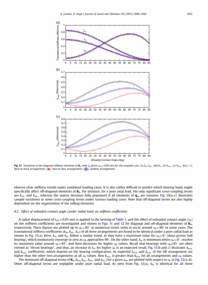
Fig. 11. Variations in the diagonal stiffness elements of Kb with α0 given δxm¼0.05 mm for the example case. (a) kxx ; kyy ; and kzz , (b) kθxθx , (c) kθyθy . Key: (◯),Back-to-back arrangement; ( ), face-to-face arrangement; ( ), tandem arrangement.


observe clear stiffness trends under combined loading cases. It is also rather difficult to predict which bearing loads mightspecifically affect off-diagonal elements of Kb. For instance, for a pure axial load, the only significant cross-coupling termsare kxθy and kyθx , whereas the matrix becomes fully populated if all elements of qm are nonzero. Fig. 10(a–c) illustratessample variations in some cross-coupling terms under various loading cases. Note that off-diagonal terms are also highlydependent on the organization of the rolling elements.

8.2. Effect of unloaded contact angle (under radial load) on stiffness coefficients

A radial displacement of δxm¼0.05 mm is applied to the bearing of Table 1, and the effect of unloaded contact angle (α0)on the stiffness coefficients are investigated and shown in Figs. 11 and 12 for diagonal and off-diagonal elements of Kb,respectively. These figures are plotted up to α0¼851 as numerical issues seem to occur around α0¼901 in some cases. Thetranslational stiffness coefficients ðkxx; kyy; kzzÞ of all three arrangements are found to be identical under a pure radial load asshown in Fig. 11(a). Here, kxx and kyy follow a similar trend, as they have a maximum value for α0¼01 (deep groove ballbearing), which nonlinearly converge to zero as α0 approaches 901. On the other hand, kzz is minimumwhen α0¼01, reachesits maximum value around α0¼651, and then decreases for higher α0 values. Recall that bearings with α0≥451 are oftenviewed as “thrust bearings”, and thus, an increase in kzz for higher α0 is an expected result. Fig. 11(b and c) illustrates kθxθxand kθyθy coefficients, which depend on the bearing configuration. As expected kθxθx and kθyθy of the DB arrangement arehigher than the other two arrangements at all α0 values. Also kθyθy is greater than kθxθx for all arrangements and α0 values.

The dominant off-diagonal terms of Kb (kxz, kxθy , kyθx , and kzθy ) for a given δxm are plotted with respect to α0 in Fig. 12(a–d).Other off-diagonal terms are negligible under pure radial load. As seen from Fig. 12(a), kxz is identical for all three

0 5 10 15 20 25 30 35 40 45 50 55 60 65 70 75 80 850

0.1

0.2

0.3

0.4

0.5

k xz (

MN

/mm

)

0 5 10 15 20 25 30 35 40 45 50 55 60 65 70 75 80 85-20

-15

-10

-5

0

5

k xθy

(MN

/rad)

0 5 10 15 20 25 30 35 40 45 50 55 60 65 70 75 80 85-5

0

5

10

15

k yθx

(MN

/rad)

0 5 10 15 20 25 30 35 40 45 50 55 60 65 70 75 80 85-25

-20

-15

-10

-5

0

k zθy

(MN

/rad)

Unloaded Contact Angle (deg)

Fig. 12. Variations in dominant off-diagonal stiffness elements of Kb with α0 given δxm¼0.05 mm for the example case. (a) kxz , (b) kxθy (c) kyθx , (d) kzθy .Key: (◯), back-to-back arrangement; ( ), face-to-face arrangement; ( ), tandem arrangement.


arrangements at all α0 and has a maximum value when α0¼451. On the other hand, kxθy , kyθx , and kzθy are dependent on thebearing arrangement and α0. One can also observe that kxθy and kzθy are negative, and kyθx ¼−kxθy .

8.3. Effect of angular position of the bearing on stiffness coefficients

So far, the stiffness elements have been calculated by assuming that the rolling elements are equally spaced along thebearing races, and the first rolling element of both rows are coincident with the x-axis (i.e. ψ i

1¼0 rad, i¼1,2). Thisassumption should be verified since the load distribution among the rolling elements changes with angular position underradial and moment loads; thus, the bearing may exhibit considerable stiffness variations.

Again, consider the same example case (of Table 1) subjected to δxm¼0.05 mm. Three diagonal stiffness elements of Kb

ðkxx; kzz; kθyθy Þ are normalized with respect to their values at ψ i1¼0 rad and plotted against the angular position of the

bearing over a complete ball passage period as shown in Fig. 13(a–c). These results are illustrated for the DB arrangement,though all arrangements show a similar behavior. As seen from Fig. 13(a–c), the stiffness elements vary between minimumand maximum values over a ball passage period. In particular, kzz shows the maximum variation (about 6 percent) over the

0 0.5 10.9995

1

1.0005

1.001

1.0015

Ball Passage Period

k xx/(

k xx)

ψ=0

k xx/(

k xx)

ψ=0

0 0.5 10.94

0.95

0.96

0.97

0.98

0.99

1

Ball Passage Period

k zz/(k

zz) ψ

=0k zz

/(kzz

) ψ=0

0 0.5 10.9995

1

1.0005

1.001

1.0015

Ball Passage Period

k θyθ

y/(k θ

yθy)

ψ=0

k θyθ

y/(k θ

yθy)

ψ=0

0 0.5 10.8

0.82

0.84

0.86

0.88

0.9

0.92

0.94

0.96

0.98

1

Ball Passage Period0 0.5 1

1

1.1

1.2

1.3

1.4

1.5

1.6

1.7

1.8

Ball Passage Period0 0.5 1

0.8

0.82

0.84

0.86

0.88

0.9

0.92

0.94

0.96

0.98

1

Ball Passage Period

Fig. 13. Variations in normalized kxx ; kzz and kθyθy over a ball passage period for back-to-back configuration given δxm¼0.05 mm for the example case.(a–c), with Z¼14 rolling elements; (d–f), with Z¼4 rolling elements.


ball passage period. The variations in kxx and kθyθy on the other hand are negligible. These results suggest that the angularposition does not have a significant effect on the stiffness elements, as the maximum variation in a stiffness coefficient is lessthan 6 percent even for a fairly large radial displacement (such as δxm¼0.05 mm).

When the variations in the stiffness elements are not small, the accuracy of the linear stiffness model decreases, andcertain kinematic parameters have a significant role in such variations. For instance, the number of rolling elements isespecially critical as it changes the ball passage period and affects the load zone of a bearing. A reduction in the number of(loaded) rolling elements extends the ball passage period and results in higher variations in the stiffness elements. Toillustrate this issue, consider an extreme case with only 4 rolling elements in each row (while all other parameters of theexample are kept the same), and calculate kxx; kzz; kθyθy for δxm¼0.05 mm. These results are shown in Fig. 13(d–f). As seenfrom the figures, kzz now shows a variation of almost 70 percent over a ball passage period, whereas the variations of kxx andkθyθy are now around 18 percent and 16 percent, respectively. These results clearly show that the angular position is animportant parameter; however, its effect can often be neglected in the presence of a sufficient number of rolling elements.

Although the variation of the stiffness elements of all arrangements are similar for a given radial load, they occurdifferently for a given moment load. Fig. 14 shows the variations in kxx; kzz and kθyθy for βym¼0.03 rad (for Z¼14). As seenfrom the figure, the variations are arrangement specific for a given βym; however, they are all within 2 percent; hence, theyare negligible.

9. Experimental validation

An experiment consisting of a vehicle wheel bearing assembly with a double row angular contact ball bearing (in theback-to-back arrangement) is designed, instrumented, and tested to experimentally validate the proposed formulation;details of this experimental study are described by the authors in a recent article [37]. The shaft-bearing experiment isanalytically described by a five degree-of-freedom model that consists of a rigid shaft (with three translational (x, y, z) and

0 0.5 10.998

1

1.002

1.004

1.006

1.008

1.01k xx

/(kxx

)=0

k xx/(k

xx)

=0k xx

/(kxx

)=0

0 0.5 10.99

0.995

1

1.005

1.01

1.015Face-to-Face Arrangement

k zz/(k

zz)

=0k zz

/(kzz

)=0

k zz/(k

zz)

=00 0.5 1

0.995

1

1.005

1.01

1.015

1.02

1.025

k/(k

yy

yy

)=0

k/(k

yy

yy

)=0

k/(k

yy

yy

)=0

0 0.5 10.995

0.996

0.997

0.998

0.999

1

1.001

0 0.5 10.985

0.99

0.995

1

1.005

1.01

1.015Back-to-Back Arrangement

0 0.5 10.99

0.995

1

1.005

1.01

1.015

0 0.5 10.999

1

1.001

1.002

1.003

1.004

1.005

1.006

1.007

0 0.5 10.992

0.994

0.996

0.998

1

1.002

1.004Tandem Arrangement

0 0.5 10.998

0.999

1

1.001

1.002

1.003

1.004

1.005

Ball Passage Period Ball Passage Period Ball Passage Period

Fig. 14. Variations in normalized kxx; kzz and kθyθy over a ball passage period given βym¼0.03 rad for face-to-face, back-to-back, and tandem configurationsof the example case.


two rotational (θx, θy) dimensions). The double row angular contact ball bearing is modeled using the proposed five-dimensional bearing stiffness matrix (Kb) with associated viscous damping (Cb). An impulse hammer test is conducted at anintermediate axial preload. Table 5 summarizes measured and predicted natural frequencies of the system (where r is the

Table 5Measured and predicted natural frequencies of the experiment, with several formulations of the analytical model.

Natural frequencies (Hz)

Modal index (r) Experiment 5 Dof model (original) 5 Dof model (with radial load) 5 Dof model (with diagonal Kb)

1 773 763 711 14222 894 763 864 14223 1636 1583 1617 15654 2049 2046 2059 16575 2246 2046 2127 1657


modal index). Observe that predictions match well with measurements, with small errors. When there is no external radialor moment load applied in the model, natural frequencies at r¼1 and r¼2, as well as r¼4 and r¼5, are repeated. With anapplication of a slight amount of load in the radial (x) direction (Fxm¼0.3 kN), these repeated roots separate as shown in thefourth column of Table 4. Now, the second, third, and fifth natural frequencies show a better match with the measurements,but the estimation of the first natural frequency deviates further from experiments.

The last column of Table 5 shows a case where a diagonal Kb (with zero cross-coupling terms) is employed in theanalytical model. In this case, the natural frequency calculations deviate significantly from measurements. These resultsclearly highlight the importance of cross-coupling stiffness terms of Kb and verify the need for a bearing stiffness matrixwhen analyzing the vibration transmission paths [4].

10. Conclusion

The chief contribution of this study is the analytical development of the fully populated five dimensional stiffness matrix(Kb) for double row angular contact ball bearings of back-to-back, face-to-face, and tandem arrangements. First, calculationsshow that it is not possible to obtain the rotational stiffness or rotational coupling terms of a double row bearing from thoseof two single row bearings, and thus a separate analytical formulation for double row bearings is absolutely essential. Usingthe proposed analytical expressions, the diagonal and non-diagonal (cross-coupling) stiffness coefficients of a double rowangular contact ball bearing are determined given either the mean displacement vector qm (by direct substitution) or themean load vector fm (by numerical solution of the nonlinear system equations). A secant method is utilized to solve themultidimensional minimization problem and the convergence issues seen in prior work [4] are minimized. The diagonalelements of the stiffness matrix are verified with a commercial code through a detailed comparison of the stiffness elementsfor an example case. Excellent agreement between the proposed model and the commercial code has been obtained underthree different loading scenarios. Then, some changes in Kb elements are further investigated with the proposed modelby varying bearing loads, unloaded contact angle, and angular position of the bearing to provide some insight. Theexperimental results (as briefly presented in this article) clearly suggest that the proposed stiffness model is valid and can beconfidently utilized for modeling double row angular contact ball bearings; further validation at this stage is not possiblesince the stiffness elements (especially the off diagonal terms) cannot be directly measured.

Considering the lack of publications on double row bearings, the new formulation provides a useful tool in the static anddynamic analyses of double row angular contact ball bearings, such as the vibration analysis of shaft-bearing assemblies.The proposed formulation is also valid for paired (duplex) bearings which behave as an integrated (double row) unit whenthe surrounding structural elements (such the shaft and bearing rings) are sufficiently rigid. The proposed theory could beextended to the analyses of double row cylindrical and tapered roller bearings as a part of the future work. In fact, themathematical formulation of angular contact ball bearings (as presented) is the most comprehensive as some of thesimplifying assumptions made for other bearing types (e.g. constant contact angle for roller type bearings) do not holdfor angular contact ball bearings.

Acknowledgments

We are grateful to the member organizations (such as the Army Research Laboratory and Honda R&D) of the SmartVehicle Concepts Center (www.SmartVehicleCenter.org) and the National Science Foundation Industry/University Coopera-tive Research Centers program (www.nsf.gov/eng/iip/iucrc) for supporting this work.

References

[1] T.A. Harris, Rolling Bearing Analysis, J. Wiley, New York, 2001.[2] J. Brändlein, P. Eschmann, L. Hasbargen, K. Weigand, Ball and Roller Bearings: Theory, Design and Application, J. Wiley, Chichester, 1999.[3] A. Palmgren, Ball and Roller Bearing Engineering, SKF Industries, Philadelphia, 1959.[4] T.C. Lim, R. Singh, Vibration transmission through rolling element bearings, Part I: bearing stiffness formulation, Journal of Sound and Vibration 139 (2)

(1990) 179–199.

www.SmartVehicleCenter.org

www.nsf.gov/eng/iip/iucrc

http://refhub.elsevier.com/S0022-460X(13)00519-1/sbref1





[5] T.J. Royston, I. Basdogan, Vibration transmission through self-aligning (spherical) rolling element bearings: theory and experiment, Journal of Soundand Vibration 215 (5) (1998) 997–1014.

[6] I. Bercea, D. Nelias, G. Cavallaro, A unified and simplified treatment of the nonlinear equilibrium problem of double-row bearings. Part I: rollingbearing model, Proceedings of the Institution of Mechanical Engineers, Part J: Journal of Engineering Tribology 217 (3) (2003) 205–212.

[7] D. Nelias, I. Bercea, A unified and simplified treatment of the nonlinear equilibrium problem of double-row bearings, Part II: application to taperrolling bearings supporting a flexible shaft, Proceedings of the Institution of Mechanical Engineers, Part J: Journal of Engineering Tribology 217 (3) (2003)213–221.

[8] Romax Technology Limited, RomaxDesigner©, ⟨www.romaxtech.com⟩, 2012.[9] F.P. Wardle, S.J. Lacey, S.Y. Poon, Dynamic and static characteristics of a wide speed range machine tool spindle, Precision Engineering 5 (4) (1983)

175–183.[10] E.P. Gargiulo, A simple way to estimate bearing stiffness, Machine Design 52 (1980) 107–110.[11] M.F. White, Rolling element bearing vibration characteristics: effect of stiffness, Journal of Applied Mechanics 46 (1979) 677–684.[12] J. Kraus, J.J. Blech, S.G. Braun, In situ determination of rolling bearing stiffness and damping by modal analysis, Journal of Vibration, Acoustics, Stress, and

Reliability in Design, Transactions of the American Society of Mechanical Engineers 109 (1987) 235–240.[13] M.D. Rajab, Modeling of the transmissibility through rolling element bearing under radial and moment loads, Ph.D. Dissertation, The Ohio State

University, 1982.[14] K. Ishida, T. Matsuda, M. Fukui, Effect of gearbox on noise reduction of geared device, Proceedings of the International Symposium on Gearing and Power

Transmissions, Tokyo, 1981, pp. 13–18.[15] J.S. Lin, Experimental analysis of dynamic force transmissibility through bearings, M.S. Thesis, The Ohio State University, 1989.[16] Y. Cao, Y. Altintas, A general method for the modeling of spindle-bearing systems, Transactions of the American Society of Mechanical Engineers, Journal

of Mechanical Design 126 (6) (2004) 1089–1104.[17] A.B. Jones, A general theory for elastically constrained ball and radial roller bearings under arbitrary load and speed conditions, Transactions of the

ASME, Journal of Basic Engineering 82 (1960) 309–320.[18] T.C. Lim, R. Singh, Vibration transmission through rolling element bearings, Part II: system studies, Journal of Sound and Vibration 139 (2) (1990)

201–225.[19] T.C. Lim, R. Singh, Vibration transmission through rolling element bearings, Part III: geared rotor system studies, Journal of Sound and Vibration 151 (1)

(1991) 31–54.[20] T.C. Lim, R. Singh, Vibration transmission through rolling element bearings, Part IV: statistical energy analysis, Journal of Sound and Vibration 153 (1)

(1992) 37–50.[21] T.C. Lim, R. Singh, Vibration transmission through rolling element bearings, Part V: effect of distributed contact load on roller bearing stiffness matrix,

Journal of Sound and Vibration 169 (4) (1994) 547–553.[22] J.M. De Mul, J.M. Vree, D.A. Vaas, Equilibrium and associated load distribution in ball and roller bearings loaded in five degrees of freedom while

neglecting frictions I: General theory and application to ball bearings, Transactions of the ASME, Journal of Tribology 111 (1989) 142–148.[23] X. Hernot, M. Sartor, J. Guillot, Calculation of the stiffness matrix of angular contact ball bearings by using the analytical approach, Transactions of the

ASME, Journal of Mechanical Design 122 (2000) 83–90.[24] P. Cermelj, M. Boltezar, An indirect approach investigating the dynamics of a structure containing ball bearings, Journal of Sound and Vibration 276 (1-2)

(2004) 401–417.[25] Y. Guo, R.G. Parker, Stiffness matrix calculation of rolling element bearings using a finite element/contact mechanics model, Mechanism and Machine

Theory 51 (2012) 32–45.[26] Advanced Numerical Solutions, Calyx© User's Manual, ⟨www.ansol.us⟩,2012.[27] T.L.H. Walford, B.J. Stone, The measurement of the radial stiffness of rolling element bearings under oscillation conditions, Proceedings of the Institution

of Mechanical Engineers, Part C: Journal of Mechanical Engineering Science 22 (4) (1980) 175–181.[28] T.L.H. Walford, B.J. Stone, Some stiffness and damping characteristics of angular contact bearings under oscillating conditions, Proceedings of the 2nd

International Conference on Vibrations in Rotating Machinery, (1980).[29] B.J. Stone, The state of art in the measurement of the stiffness and damping of rolling element bearings, Annals of the CIRP 31 (2) (1982) 529–538.[30] E.R. Marsh, D.S. Yantek, Experimental measurement of precision bearing dynamic stiffness, Journal of Sound and Vibration 202 (1) (1997) 55–66.[31] R. Tiwari, N.S. Vyas, Estimation of nonlinear stiffness parameters of rolling element bearings from random response of rotor-bearing systems, Journal

of Sound and Vibration 187 (1995) 229–239.[32] G. Pinte, S. Devos, B. Stallaert, W. Symens, J. Swevers, P. Sas, A piezo-based bearing for the active structural acoustic control of rotating machinery,

Journal of Sound and Vibration 329 (9) (2010) 1235–1253.[33] M. Cao, J. Xiao, A comprehensive dynamic model of double-row spherical roller bearing – model development and case studies on surface defects,

preloads, and radial clearance, Mechanical Systems and Signal Processing 22 (2008) 467–489.[34] M. Cao, A refined double-row spherical roller bearing model and its application in performance assessment of moving race shaft misalignments,

Journal of Vibration and Control 13 (2007) 1145–1168.[35] D.H. Choi, K.C. Yoon, A design method of an automotive wheel-bearing unit with discrete design variables using genetic algorithms, Journal of

Tribology 123 (2001) 181–187.[36] A. Gunduz, Multi-dimensional stiffness characteristics of double row angular contact ball bearings and their role in influencing vibration modes, Ph.D.

Dissertation, The Ohio State University, 2012.[37] A. Gunduz, J.T. Dreyer, R. Singh, Effect of bearing preloads on the modal characteristics of a shaft-bearing assembly: experiments on double row

angular contact ball bearings, Mechanical Systems and Signal Processing 31 (2012) 176–195.[38] W. Xu, T. Coleman, G. Liu, A secant method for nonlinear least-squares minimization, Computational Optimization and Applications 51 (1) (2012)

159–173.








www.romaxtech.com



























www.ansol.us



















journal of sound and vibration - acoustics and dynamics ... and...stiffness matrix formulation for...

Documents