journal of earth and atmospheric research

A GEOSTATISTICAL RISK ASSESSMENT OF THE HYDROCARBON POTENTIAL IN “AMESERE” FIELD, NIGER DELTA, NIGERIA

Journal of Earth and Atmospheric ResearchTE EC CH NN AO ILL EOG RY F F ELOR S

Falebita, D. E., Osotuyi, A. G. and Akinsanpe, O. T.

Department of Geology, Obafemi Awolowo University, Ile - Ife, Nigeria

1Falebita et al/JEAR 1 (1) (2018) (1-15)

D ATMN O AH SPT HR EA RE IF C O R EL SA EN AR RU C

O HJ

Article History

Keywords:Geosta�s�cal, Risk,Assessment, Well logs,Niger Delta, Nigeria

Received: May 2, 2018Revised: June 10, 2018Accepted: June 30, 2018

ABSTRACT

This study assessed two hydrocarbon reservoirs A and B in 'AMESERE' Field within the Miocene Agbada Formation by utilizing quantitative, deterministic and stochastic simulation workflows on some petrophysical parameters (gross pay, net pay, porosity and water saturation) obtained from irregularly distributed 24 well logs that penetrated the reservoirs. This was with a view to modelling the spatial variability and field-wide extrapolated heterogeneity models of the reservoir across the study area. Average unbiased estimation maps constrained by exponential variogram models of the parameters data were produced and used as inputs for Sequential Gaussian Simulation (SGSIM), a modelling algorithm to produce fifty (50) equally probable realizations. These were used to risk the parameters at different probability levels. In reservoir A at P10, P25, P50, P75 and P90, simulated gross pay was between 11.13 and 22.29 m; net pay was between 2.41 and 13.50 m; porosity was between 18.00 and 33.00%; and water saturation was between 14.02 and 74.96% respectively. In reservoir B at P10, P25, P50, P75 and P90, simulated gross pay was between 17.85 and 57.28 m; net pay was between 5.55 and 49.64m; porosity was 22.00 and 33.00%; and water saturation was between 10.57 and 88.77% respectively. These results are consistent with geostatistical modelling because they show different plausible realizations that quantify varying risks in the distribution of the petrophysical data within the reservoirs.

1.0 Introduction Subsurface property estimation from remote geophysical measurements is always subject to uncertainty, due to many inevitable difficulties and ambiguities in data acquisition, processing, interpretation and insufficient data sets (Avseth, et al., 2007; Schiozer, et al., 2004). Hence, uncertainty and heterogeneity delineation is a key factor in reliable reservoir characterization. Geostatistics employs statistical approach to provide solutions to problems covering broad geological and environmental areas (Zamani and Mirabadi 2011; Caridad and Jury 2013; Gorai and Kumar 2013; Méli'i et al. 2013; Nshagali et al. 2015; Arétouyap et al. 2015). Its distinctive feature is its inclination towards

spatial characterization as opposed to traditional sampling techniques, tailored to eliminate spatial dependencies (Hack, 2005). This in turn provides a probabilistic means to reliably estimate a set of data, where samples are not observed (Deutsch, 2002). With geostatistical simulations, geologically reasonable spatial correlation and small-scale variability are added (Caers, 2000; Shiozer, et al., 2004; Avseth, et al., 2007; Bohling, 2007). The results must be interpreted and validated in light of reservoir g e o l o g y a n d a v a i l a b l e r e s e r v o i r information/principles (Chambers et. al., 2000). This study, therefore, seeks to model the spatial variability and field-wide extrapolated heterogeneity characteristics

of the parameters of two hydrocarbon reservoirs in “AMESERE” Field using geostatistical estimation and simulation techniques on 24 irregularly spaced wells. This is with the aim to achieving both s ta t is t ical and spat ia l representation in the estimation and simulation of the parameters beyond well controls. The results would guide the decision making process for cautious and optimal hydrocarbon exploitation from the two reservoirs.

2.0 REGIONAL GEOLOGIC SETTING AND STRATIGRAPHY OF THE NIGER DELTA

The Niger Delta oil and gas province is located in Southern Nigeria between Latitudes 40N and 60N and Longitudes 30E and 90E (Nwachukwu and Chukwura, 1986). The Tertiary Niger Delta covers an area of approximately 75,000km2 (46, 575 mi2) and estimated to be 9000 12000m (29,529 39,372 ft) thick. It is bounded by the Abakaliki Trough in the Northeast (Short and Stauble, 1967; Merki, 1972). Westward, the delta complex merges across the Benin Hinge Line and Okitipupa High into Dahomey Basin. In the East, the delta is bounded by a line of volcanic rocks, comprising the Cameroon volcanic zone and Guinea ridge (Ete-Efeotor, 1997) with structures like the Calabar Flank. The Chain and Charkot oceanic transform faults propagation controlled Niger Delta subsidence (Reijers, 1996). The southward progradation of the Niger Delta was accomplished by a stepwise

build-out of fluvio-marine offlap sequences controlled by subsidence along synsedimentary faults, and punctuated by rapid shifts from depobelts to the next (Fig. 1a). These sudden shifts, recognized by the rapid seaward advance of alluvial sands over the thick paralic sequence, form the escalator regressive style (Knox and Omatsola, 1989). The main characteristic of this regression the rapid advance of alluvial sands is due to the cessation of subsidence in a depobelt and the continuation of sediment supply (Doust and Omatsola, 1990). Short and Stauble (1967) first named the three subsurface units as Akata, Agbada and Benin Formations (bottom to top), in the Cenozoic Niger Delta (Fig 1b). The Akata Formation consists of dark-grey, marine, pro-delta shales, which are often overpressured while the Agbada Formation is a paralic sequence, characterised by intercalation of sandstones and shales. It is the main hydrocarbon-bearing formation in the Niger Delta. Growth faults partly influence variations in thicknesses and depths to sand bodies. The Benin Formation is the topmost unit and is mostly continental, freshwater-bearing sands. All the formations are diachronous and range in age from Eocene to Holocene (Fig. 1b). The 'AMESERE' Field (Fig 1c) lies in the shallow offshore, western Niger Delta. The field is situated within the paleogeographic zone refered to as the Upper Miocene/ Pliocene/ Pleistocene of the delta formation cycle (Etu-Efetor, 1997).

2 Falebita et al/JEAR 1 (1) (2018) (1-15)

A Geosta�s�cal Risk Assessment of the Hydrocarbon Poten�al in “Amesere” Field, Niger Delta, Nigeria

Falebita et al

3.0 METHODOLOGY

3.1 B A S I C C O M P U T A T I O N O F SAMPLED RESERVOIR PARAMETERSThe reservoir parameters, namely, gross pay (Gpay), net pay (NPay), porosity (Φ), and water saturation (Sw) were intially calculated from the combined use of gamma ray, resistivity, density and neutron logs, from the 24 well logs.

3.1.1 POROSITY (Φ)The porosity was computed by averaging the value from the measurements obtained from the neutron porosity (ΦN) and the density (ΦD) logs using equation 1.

(1)

Where Φ is the computed porosity.

3.1.2 WATER SATURATIONWater saturation (Sw) was obtained from electrical logs via Archie's equation:

(2)

Where the true resistivity of the formation, F is the formation factor and Rw resistivity of the formation water.

Figure 1: (a) Niger Delta regional map of the escalator-like geometry forming six depobelts (after Knox and Omatsola 1989; Doust and Omatsola, 1990) and (b): Stratigraphic column of the Formations of the Niger Delta (after Doust and Omatsola, 1990). (c) Location map of the study area



Falebita et al

Φ = ( N - DΦ Φ2 2

( - 2

0.5

= -

SwFRw

Rt-

3.1.3 GROSS PAY (GPAY)

The gross pay was obtained using the combination of the gamma ray and the resistivity logs for the hydrocarbon bearing i n t e r v a l s . I t i s t h e t h i c k n e s s o f t h e stratigraphically defined interval in which the reservoir beds occur, including such non-productive intervals interbedded between the productive intervals.

3.1.4 NET PAY (NPAY)

The net pay was obtained using the combination of the gamma ray and the resistivity logs for the hydrocarbon bearing intervals. It is the thickness of those intervals in which porosity and permeability are known or supposed to be high enough for the interval to be able to produce oil or gas.

3.2 GEOSTATISTICAL ANALYSIS OF THE RESERVOIR PARAMETERS

The geostatistical analysis of the reservoir parameters above was achieved in three steps (1) variogram modelling, (2) estimation using ordinary kriging (OK), and (3) simulation using the sequential Gaussian simulation (SGSIM) method. The reservoir data sets were set up in the Geostatistical Library (GSLIB) format (Bohling, 2007). It adopted a simple American Standard Code for Information Interchange (ASCII).

3.2.1 VARIOGRAM MODELLING

A semivariogram is a statistically based quantitave description of a surface used for the characterization of spatial continuity, roughness and correlation of a dataset (Bohling, 2007). Its characteristics include the range, sill nugget and distance (Chilès and Delfiner 2012). Range is

the lag distance (h) at which the variogram (or semivariogram component) reaches the sill value. This is the distance, h from the origin to the point where the model reaches a constant value or sill. The range is the distance after which the variogram levels off. The physical meaning of the range is that pairs of points that are this distance or greater apart are not spatially correlated. The sill represents the maximum variance. It is the total variance contribution, or the maximum variability between pairs of data pairs; at the point where the sill levels off, there is no longer variation (spatial relationship) between data pairs. The nugget is the y-intercept of the variogram. It represents the short range variability (noise) in the data. Other acceptable models are spherical, exponential, Gaussian, power and nugget effect models (Remy, 2004; Bohling, 2007; Remy et. al., 2009; Chilès and Delfiner 2012). They must be technically non-negative definite for the system of kriging equations to be non-singular (Ubulom and Nwachukwu, 2014). Empirical spherical and exponential semivariogram models were fitted to the calculated reservoir parameters interactively with no significant difference. In practice, only the experimental variogram (Equation 3) is calculated from observed (existing) data.

(3)

where γ(h) is the estimated value of the semivariogram for lag (h); N(h), the number of pairs of points separated by distance h; z(uα) and z(uα + h) are values of z at positions uα and uα +

h, respectively. For w= 2, semivariogram;

madogram ( w= 1); and rodogram ( w= ½) (Deutsch and Journel, 1992). However, in this s tudy, the exponential model def ined mathematically in Equation 4 was employed for the kriging and simulation processes in this

=

+-=)(

1

)()()(2

1)(

hN

huzuzhN

ha

w

aag



Falebita et al

work.

(4)

Where c = contribution or sill (a measure of variance), a = practical range, h = lag distance. The three parameters are of interest because they serve as inputs to the ordinary kriging estimation and sequential simulation.

3.2.2 ESTIMATION USING ORDINARY KRIGING TECHNIQUE

Kriging is an optimal interpolation process that generates (using observed data) best linear unbiased estimate (BLUE) at a new location where there is/are no observed data (Bohling, 2005). It employs semivariogram model. Kriging assigns weights to a data-driven weighting function, not arbitrary function, while it remains an interpolation algorithm, yielding results close to others in many cases (Isaaks and Srivastava, 1989). Kriging gives us an estimate of both the mean and standard deviation of the variable at each grid node, meaning that we can represent the variable at each grid node as a random variable following a normal (Gaussian) distribution. There are four (4) types of kriging: simple kriging (SK), Ordinary kriging (OK), kriging with polynomial trend (KT) and simple kriging with a locally varying mean (LVM) (Goovaerts, 1997; Pebesma, 2003; Bohling, 2007; Remy et. al., 2009). The ordinary kriging was used in this work for the deterministic estimation. It is considered to be the most straight-forward since it is the only algorithm that can compute from semi-variogram (or co-variogram) relationship without having to provide additional qualifying data or pre- or

post-manipulation of the sample data or kriging results (Krige, 1996; David, 1977; Bohling, 2005; Falebita et al., 2014). The ordinary kriging estimates the value of a point from a set of nearby random variables (Isaaks and Srivastava, 1989). The system includes linear equations with unknowns such that:

(5)

Where K is the matrix of covariances between

data points with elements K = C (u -u ). k is a,b R a b

the vector of covariances between the data points and the estimation point with elements

given by K = C (u -u) and l (u) is the vector of a R a ok

ordinary kriging weights for the surrounding data points (Krige, 1996; Bohling, 2007).

-1Multiplying K by K will downweight points falling in clusters relative to isolated points at the same distance (Krige, 1996; Bohling, 2007).

3 . 2 . 3 S E Q U E N T I A L G A U S S I A N SIMULATION TECHNIQUE (SGSIM)

Simulation is the process of building alternatively equally probable realizations based on spatial distribution of a variable and it provides alternative numerical models, each being a good representation of the reality (Bohling, 2007; Cabello et al., 2007). The alternative realizations provided through simulation permit determination of differences and are measures of joint spatial uncertainty. Rather than choosing the mean as the estimate at each node, the SGSIM chooses a random deviate from this normal distribution, selected according to a uniform random number representing the probability level (Srivastava, 1994; Hohn, 1988; Bohling, 2007). The SGSIM employs the mean and variance of kriging in



Falebita et al

g(h)=c [1 - exp ( - 3h )]- a

-1l (u) = K k0k

which the trend component is assumed to be constant and mean is known. It is a form of simulation tool used for continuous variables like porosity, permeability, water saturation etc. The basic steps in the SGS process are to (1) generate a random path through the grid nodes, (2) visit the first node along the path and use kriging to estimate a mean and standard deviation for the variable at that node based on surrounding data values, (3) select a value at random from the corresponding normal distribution and set the variable value at that node to that number, and (4) visit each successive node in the random path and repeat the process, including previously simulated nodes as data values in the kriging process. The random path is to avoid artifacts induced by walking through the grid in a regular fashion. While the inclusion of previously simulated grid is to preserve the proper covariance structure between the simulated values (Hohn, 1988; Srivastava, 1994; Bohling, 2007). Fifty realizations of the computed reservoir properties were simulated.

4.0 Results and Discussion

4.1 I n i t i a l l y C o m p u t e d R e s e r v o i r ParametersTable 1 contains minimum, maximum and average reservoir parameters initially obtained

on the two reservoirs from 24 wells. The tops and bases of the reservoir A range between 1716 m and 2067 m; while they range between 1821 m and 2123 m in reservoir B respectively. The gross pay ranges between 3 m and 17 m in reservoir A with an average of about 12 m and between 6 m and 57 m in reservoir B with an average of about 24 m. The gross pay interval is twice as big in reservoir B compared to reservoir A.

The net pay ranges between 2 m and 14 m in reservoir A with an average of 7.2 m and between 6 and 50 m in reservoir B with an average of 22.8 m. The net pay interval which is of interest is approximately thrice as big in reservoir B compared to reservoir A. The porosity values range between 18 and 33% in reservoir A with an average of 25.9% and between 22% and 33% in reservoir B with an average of 27.2%. The water saturation ranges between 14% and 75% in reservoir A with an average of 41.4% and between 20% and 89% in reservoir B with an average of 59.6%. These average values are only statistically and not necessarily spatially correlative. Hence, their limitation to within well locations. Figure 2 is a representative display of the correlation of the two reservoirs across three wells, namely AME 19, 21 and 22. The two reservoirs are hydrocarbon bearing with water dominating


Falebita et al


Reservoir A Top (m) Base (m)

Gross Pay (m)

Net Pay (m)

Porosity (%) Water Saturation (%)

Average 1812.82 1830.05 12.16 7.16 25.9 41.4

Minimum 1716 1735 3 2 18 14

Maximum 2067 2085 17 14 33 75

Reservoir B Top (m) Base (m)

Gross Pay (m)

Net Pay (m)

Porosity (%) Water Saturation (%)

Average 1908.43 1940.49 24.12 22.84 27.2 59.6

Minimum 1821 1855 6 6 22 20

Maximum 2123 2145 57 50 33 89

Table 1: Initially computed average reservoir parameters from 24 wells

4 . 2 M E A S U R E S O F G E O L O G I C CONTINUITYFigure 3 shows the experimental variogram models which are measures of geologic continuity with lag (distance) for the four different parameters, namely gross pay, net pay, porosity and water saturation in reservoirs A and B. The horizontal and vertical dotted lines

represent the sills and ranges respectively.

The range represents maximum limit of distance of usefulness of the data while the sill represents maximum variance in the data set. The geologic continuity varies as expected for the parameters with lag distances in each reservoir. In reservoir

Figure 2: Lithologic correlation of reservoirs A and B using gamma ray and resistivity logs across representative three wells.

The range represents maximum limit of distance of usefulness of the data while the sill represents maximum variance in the data set. The geologic continuity varies as expected for the parameters with lag distances in each reservoir. In reservoir A, the gross pay has a sill of 304,000 and range of 3750 m; net pay has a sill of 200,000 and range of 3000 m; porosity has a sill of 290,000 and range of 2900 m; while water saturation has

a sill of 300,000 with a range less than 2500 m. In reservoir B, the experimental variogram model for gross pay has a sill of 235,000 and range is about 1200 m; net pay has a sill of 200,000 with a range of about 1100 m; porosity has a sill of 230,000 with a range of about 1300 m; while water saturation shows the sill contribution of 265,000 with a range of about 1100 m.


Falebita et al


The variance (sill effect) is generally higher and the range longer for the parameters measured in reservoir A compared to reservoir B. The implication is that variability in parameter estimation is expected to be higher and much more extensive in reservoir A compared to reservoir B.

4.3 THE AVERAGE UNBIASED ESTIMATESThe deterministic estimates (ordinary kriging estimation) constrained by the variogram models give average unbiased outlooks of the different parameters in each reservoir (Figures 4 and 5). The estimates are statistically and spatially correlated/constrained beyond well controls.

Figure 3: Experimental variogram models for the gross pay, net pay, porosity and water saturation for reservoir A and reservoir B where the horizontal and vertical dotted lines represent the sills and ranges respectively.


Falebita et al


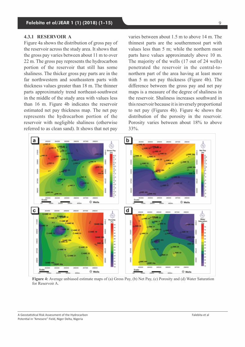
4.3.1 RESERVOIR AFigure 4a shows the distribution of gross pay of the reservoir across the study area. It shows that the gross pay varies between about 11 m to over 22 m. The gross pay represents the hydrocarbon portion of the reservoir that still has some shaliness. The thicker gross pay parts are in the far northwestern and southeastern parts with thickness values greater than 18 m. The thinner parts approximately trend northeast-southwest in the middle of the study area with values less than 16 m. Figure 4b indicates the reservoir estimated net pay thickness map. The net pay represents the hydrocarbon portion of the reservoir with negligible shaliness (otherwise referred to as clean sand). It shows that net pay

varies between about 1.5 m to above 14 m. The thinnest parts are the southernmost part with values less than 5 m; while the northern most parts have values approximately above 10 m. The majority of the wells (17 out of 24 wells) penetrated the reservoir in the central-to-northern part of the area having at least more than 5 m net pay thickness (Figure 4b). The difference between the gross pay and net pay maps is a measure of the degree of shaliness in the reservoir. Shaliness increases southward in this reservoir because it is inversely proportional to net pay (Figures 4b). Figure 4c shows the distribution of the porosity in the reservoir. Porosity varies between about 18% to above 33%.

Figure 4: Average unbiased estimate maps of (a) Gross Pay, (b) Net Pay, (c) Porosity and (d) Water Saturation for Reservoir A.


Falebita et al


The majority of the wells (except AME 25 and AME 35) are located on the parts that have more than 23% porosity. Figure 4d shows the water saturation distribution in the reservoir. The water saturation varies between 10% in the northeastern part and over 75% in the

northwestern part of the area. In other words, hydrocarbon saturation is highest (about 90%) in the northeastern part compared to the northwestern end of the study area where it is about 25%. The porosity and hydrocarbon saturation are increasing northeastward.

Figure 5: Average unbiased estimate maps of (a) Gross Pay, (b) Net Pay, (c) Porosity and (d) Water Saturation for Reservoir B

4.3.2 RESERVOIR BIn reservoir B, Figure 5a is the distribution of gross pay of the reservoir across the study area. It shows that the gross pay varies between 16 m and about 60 m. The gross pay generally increases northeastward. More wells (about 13 wells) penetrated the reservoir at portions with above 30 m gross pay compared to portions below 30 m. Figure 5b indicates the reservoir estimated net pay thickness map. It shows that

net pay varies between about 4 m and above 54 m. The northeastern part has the thickest net pay (about 38 m) while the southwestern part has the thinnest net pay (below 20 m). The net pay is generally similar to the gross pay map in distribution pattern for this reservoir. The shaliness (difference between the gross pay and net pay) is about 12 m in the southwestern part but less than 7 m in the northeastern part of the area. In other words, shaliness increases


Falebita et al


southwestward. The majority of the wells (16 out of 24 wells) penetrated the reservoir at portions with net pay thickness more than 20 m. Figure 5c shows the distribution of the porosity in the reservoir. Porosity varies between 22% and above 33%. Ten of the wells penetrated the reservoir at portions with less than 26% porosity. Figure 5d shows the water saturation distribution in the reservoir. The water saturation varies between 15% and 90% in the reservoir. The hydrocarbon saturation is highest (about 85%) at the centre compared to other places. This central part with less than 26% porosity has higher hydrocarbon saturation probably due to local uplift or heterogeneity effect as a result of differential compaction within the reservoir.

4.4 ASSESSMENT OF PARAMETERS AT DIFFERENT RISK LEVELSUnlike the deterministic estimates of the reservoir parameters which give average values, the stochastically simulated parameters give a measure of risk of the estimated values. The probability distributions of the reservoir parameters are presented in percentiles (Table 2). P10 and P25 represent 10% and 25% risk a parameter would be less than a given threshold respectively; P75 and P90 represent 25% and 10% risk a parameter would be more than a given threshold; while P50 which indicates 50% means equal chance of being less or more than a given threshold.

In reservoir A, at P10 there is a 10% risk of having a gross pay less than the range of 11.13 11.27 m; net pay less than 2.41 2.70 m; porosity less than 18.00 18.49% and water saturation less than 14.02 14.38% respectively. At P25, there is a 25% risk of encountering gross pay less than the range of 13.08 14.90; net pay

less than 4.49 6.40 m; porosity less than 20.28 27.12%; and water saturation less more than 27.12 31.74% respectively. At P50 there is an equal chance (50%) of having gross pay less or more than the range of 16.07 -17.58 m; net pay less or more than 7.01 -10.50 m; porosity less or more than 24.29 27.00%; and water saturation is less or more than 41.55 - 47.17% respectively. At P75, there is a 25% risk of having gross pay more than the range of 18.62 20.28 m; net pay more than 9.96 13.50 m; porosity more than 27.61 30.10%; and water saturation more than 50.25% - 62.08% respectively. At P90, there is a 10% risk that the gross pay is more than 22.17 22.29 m; net pay more than 13.07 13.50 m; porosity more than 32.55 33.00%; and water sa tura t ion more than 74 .41 74 .96% respectively.

Similarly in reservoir B, there is a 10% (P10) risk of having gross pay less than the range of 17.85-19.64 m; net pay less than of 5.55 - 5.78 m; porosity less than of 22.00 - 22.15% and water saturation less than 10.57 - 19.91% respectively. At P25, there is a 25% risk that the gross pay is less than the range of 25.11 - 30.18 m; net pay less than 15.22 - 17.92 m; porosity less than 24.09 - 25.65%; and water saturation less than 33.91 - 39.01% respectively. At P50 there is an equal chance of having gross pay less or more than the range of 33.25 - 39.82 m; net pay less or more than 26.95 - 29.07 m; porosity less or more than 26.73 - 28.23%; and water saturation is less or more than 50.24 - 56.25% respectively. At P75, there is a 25% risk of having gross pay more than the range of 41.75 - 49.75 m; net pay more than 37.05 - 40.49 m; porosity more than 29.45 - 30.80%; and water saturation more 68.33 - 73.43%. At P90, there is a 10% risk that the gross pay would be more than 56.50 - 57.28 m; net pay more than 49.39 - 49.64


Falebita et al


m; porosity more than 32.72 - 3.00%; and water saturat ion more than 88.23 - 88.77% respectively.

The significance of these analyses is that at any given point in the reservoirs over the study area, there is a quantifiable level of risk (or uncertainty) associated with any estimated reservoir value which must be factored into immediate and future decision making process regarding the reservoirs for cautious and optimal hydrocarbon exploitation.

5.0 CONCLUSIONSThe spatial distribution and risks associated with the reservoir properties of two variably thick, hydrocarbon reservoirs within the 'Amesere' Field have been assessed using the geostatistical techniques. The geostatistical techniques involved quantification of geologic continuity with the variogram models, determination of deterministic unbiased estimates using the

Table 2: Stochastically simulated reservoir parameters at different risk levels for reservoirs A and B


Falebita et al


Parameter/Reservoir Reservoir A Reservoir B

Gross Pay (meters) Probability Minimum Maximum Minimum Maximum

P10 11.13 11.27 17.85 19.64

P25 13.08 14.90 25.11 30.18 P50 16.07 17.58 33.25 39.82 P75 18.62 20.28 41.75 49.75 P90 22.17 22.29 56.50 57.28

Net Pay (meters)

Probability Minimum Maximum Minimum Maximum

P10 2.41 2.70 5.55 5.78 P25 4.49 6.40 15.22 17.92 P50 7.01 10.50 26.95 29.07

P75 9.96 13.50 37.05 40.49 P90 13.07 13.50 49.39 49.64

Porosity (%)


P10 18.00 18.49 22.00 22.15 P25 20.28 27.12 24.09 25.65 P50 24.29 27.00 26.73 28.23 P75 27.61 30.10 29.45 30.80 P90 32.55 33.00 32.72 33.00

Water Saturation (%)


P10 14.02 14.38 10.57 19.91 P25 27.12 31.74 33.91 39.01 P50 41.55 47.17 50.24 56.25 P75 50.25 62.08 68.33 73.43 P90 74.41 74.96 88.23 88.77

ordinary kriging and conditional simulation using the sequential Gaussian simulation technique. The study provided probable interwell distribution, variabilities and risks associated with the reservoir data distribution in the two reservoirs over the study area on and beyond well controls. The random combination of these parameters at different risk levels appraises the risks associated with the hydrocarbon potential of the field. These results are consistent with geostatistical modelling that could help with optimum decision on field hydrocarbon prospectivity.

ACKNOWLEDGMENTS

The authors gratefully acknowledge the management of Department of Petroleum Resources, for making this data available. Also the various Oil Companies that provided the workstations/software in the Department of Geology, Obafemi Awolowo University, Ile-Ife and Stanford University Center for Reservoir Forecasting (SCRF) for making available the SGeMS as an open source software.

REFERENCES

Arétouyap, Z., Nouayou, R., Njandjock, N. P. a n d A s f a h a n i , J . 2 0 1 5 : A q u i f e r s productivity in the Pan-African context. Earth Syst Sci. vol.124, 3, pp 527539. Doi: 10.1007/s12040-015-0561-1.

Avseth, P., Mukerji, T. and Mavko, G. 2007: Quantitative Seismic Interpretation: Applying Rock Physics Tools to Reduce Interpretation Risk. Cambridge University Press, UK.

Bohling, G., 2005: Introduction to Geostatistics and Var iog ram Ana lys i s . Kansas Geological Survey Open File Report www.http://people.ku.edu/~gbohling/.

Bohling, G. 2007: Introduction to Geostatistics. Kansas Geological Survey Open File Report no.26, 50p.

Cabello, P., Cuevas, J. L. and Ramos, E. 2007: 3D Modelling of Grain Size distribution in Quaternary Deltaic Deposits, Llobregat Delta, NE Spain. Geological Acta, vol. 5, 3, pp.231-244.

Caers, J. 2000: Direct sequential indicator simulation. Stanford Centre for Reservoir Forecasting, vol. 11, Stanford, USA.

Caridad, R. P. and Jury, M. R. 2013: Spatial and temporal analysis of climate change in Hispañola. Theor Appl Climatol., vol. 113, pp. 213224. Doi: 10.1007/s00704-012-0781-0.

Chambers, R. L., Yarus, J. M. and Hird, K. B. 2000: Petroleum Geostatistics for Non-geostaticians, Part 2, Leading Edge, 19, pp. 592592

Chilès, J. P and Delfiner, P. 2012: Geostatistics: Modeling Spatial Uncertainty. 2. New York: Wiley, 734pp.

David, M. 1977: Geostatistical Ore Reserve Estimation, 2nd edition, Elsevier, 364 pp.

Deutsch, C.V., and Journel, A. G. 1992: Geostatistical software library and user's guide. Oxford University Press, New York. 340 pp.

Deutsch, C. V. 2002: Geostatistical Reservoir Modelling, Oxford University Press, 376pp.

Doust, H., and E. Omatsola, (1990): Niger Delta, in J. D. Edwards, and P. A. Santogrossi, eds., Divergent/passive margins basins: AAPG Memoir 48, p. 201238


Falebita et al


Etu-Efeotor, J. O. (1997): Fundamentals of Petroleum Geology. Paragraphics, Port Harcourt, p.146.

Falebita, D. E., Oyebanjo, O. M. and Ajayi, T. R. (2014): A geostatistical review of the Bitumen reserves of the Upper Cretaceous Afowo Formation Agbabu Area, Ondo State, Eastern Dahomey Basin, Nigeria, Petroleum and Coal, vol 56, 5, pp .572-581, 201

Goovaerts, P. 1997: Geostatistics for Natural Resources Evaluation, Oxford University press, New York, 483 pp.

Gorai, A. K and Kumar, S. 2013: Spatial distribution analysis of groundwater quality index using GIS: a case study of Ranchi municipal corporation (RMC) area. Geoinf Geostat Overv.

Hack, D. R. 2005: Issues and Challenges in the application of Geostatistics and Spatial-Data analysis to the Characterization of Sand and Gravel Resources. In: Bliss, J. D., Moyle, P. R., and Long, K. R., (eds), Chapters of Contributions to Industrial Minerals Research, Bulletin 2209-J, p.1-14..

Hohn, M. E. 1988: Geostatistics and Petroleum Geology, Van Nostrand Reinhold, NY, 264 pp. Srivastava, R. M., 1994a, “An Overview of Stochastic Methods for Reservoir Characterization,” In Stochastic Modeling and Geostatistics, (1994), J. M. Yarus and R. L. Chambers, Eds., AAPG Computer Applications in Geology, No. 3, pp. 3-16.

Isaaks, E. H. and Srivastava, R. M. 1989: An Introduction to Applied Geostatistics: Ney York, Oxford University Press, 561pp.

Knox, G. J., and Omatsola, E., (1989): Development of the Cenozoic Niger Delta in terms of the Escalator Regression Model and Impact on Hydrocarbon Distribution. Proceedings KNGMG Symposium, C o a s t a l L o w l a n d s G e o l o g y a n d Geotechnology, The Hague Kluwer Academy Publi. (Dordrecht): 182

Krige, D. G. 1996: A practical analysis of the effects of spatial structure and of data available and accessed on the conditional bases in ordinary kriging. Geostatistics Wollongong, (Eds Baafi , E Y and Schofield, N A,) Kluwer, pp799 810.

Merki, P. (1972). Structural geology of the Cenozoic Niger Del ta . In T. F. J Dessauvagie and A. J. Whiteman (Eds) Africa Geology Univ. of Ibadan Press. 635 645.

Méli'I, J. L., Bisso, D., Njandjock N. P., Ndougsa, T., Mbanga A. F., Manguelle-Dicoum, E. 2013: Water table control using ordinary kriging in the southern part of Cameroon. J Appl Sci. vol. 13, pp. 393400. Doi: 10.3923/jas.2013.393.400.

Nshagali, B. G., Njandjock, N. P., Meli'I, J. L., Arétouyap, Z. and Manguelle-Dicoum, E. 2015: High iron concentration and pH change detected using statistics and geostatistics in crystalline basement equatorial region. Environ Earth Sci. vol 73:71357145. Doi: 10.1007/s12665-014-3893-2.

Nwachukwu J. I. and Chukwura P. I. (1986): Organic Matter of Agbada Formation, N i g e r D e l t a , N i g e r i a . A m e r i c a n Association of petroleum Geologist Bulletin, vol. 70, 6, pp. 48-55.


Falebita et al


Pebesma, E. J. 2003: Gstat: Multivariable Geostatistics for S. Proceedings of the 3rd International Workshop on Distributive Statistical Computing (DSC, 2003) March 20 22, Vienna, Austra. ISSN 1609-395X.

Reijers, T. J. A. 1996: Selected Chapters on Geology, Sedimentary Geology and Stratigraphy in Nigeria. Shell Petroleum Development Company, p. 103-117.

Remy, N. 2004: The Stanford Geostatistical S o f t w a r e . U s e r ' s M a n u a l : http://SGEMS.sourceforge.net/doc/SGeMs_manual.pdf.

Remy, N., Boucher, A. and Wu, J. 2009: Applied Geostatistics with SGeMS, Cambridge University Press, 264pp.

Schiozer D. J., Ligero E. L. and Santos, J. A. M. 2 0 0 4 : A s s e s s m e n t f o r R e s e r v o i r Development under Uncertainty. J. of the Braz. Soc. of Mech. Sci. & Eng. vol. 26, 2, pp. 213 217.

Short, K. C. and Stäublee, A. J. 1965: Outline of geology of Niger Delta: American Association of Petroleum Geologists Bulletin, v. 51, p. 761-779.

Srivastava, R. M. 1994: “An Overview of Stochast ic Methods for Reservoir Characterization,” in Stochastic Modeling and Geostatistics, (1994), J. M. Yarus and R. L. Chambers, Eds., AAPG Computer Applications in Geology, No. 3, pp. 3-16.

Ubulom, D. E. N. and Nwachukwu, J. I. 2014: Geostatistical Modelling of Log Derived Quantitative Lithofacies Data, Offshore Niger Delta, Nigeria Association of Petroleum Explorationists Bulletin, vol. 26, 2, pp 51-66.

Z a m a n i , A . a n d M i r a b a d i , A . 2 0 11 : Optimization of sensor orientation in railway wheel detector, using kriging method. J Electromagn Anal Appl., 3, pp 529536.


Falebita et al


journal of earth and atmospheric research

Documents