journal of applied geophysics geophysics_jog_2017.pdfa environmental geophysics associates, austin,...

Journal of Applied Geophysics 138 (2017) 114–126

Contents lists available at ScienceDirect

Journal of Applied Geophysics

j ourna l homepage: www.e lsev ie r .com/ locate / j appgeo

Integrated geophysical investigations of Main Barton Springs, Austin,Texas, USA

By Mustafa Saribudak a,⁎, Nico M. Hauwert b

a Environmental Geophysics Associates, Austin, TX, United Statesb City of Austin Watershed Protection Department, Austin, TX, United States

⁎ Corresponding author.E-mail addresses: [email protected] (B.M. Saribudak), Nico

(N.M. Hauwert).

http://dx.doi.org/10.1016/j.jappgeo.2017.01.0040926-9851/© 2017 Elsevier B.V. All rights reserved.

a b s t r a c t
a r t i c l e i n f o
Article history:Received 16 July 2015Received in revised form 15 December 2016Accepted 4 January 2017Available online 8 January 2017

Barton Springs is a major discharge site for the Barton Springs Segment of the Edwards Aquifer and is located inZilker Park, Austin, Texas. Barton Springs actually consists of at least four springs. The Main Barton Springs dis-charges into the Barton Springs pool from the Barton Springs fault and several outlets along a fault, from acave, several fissures, and gravel-filled solution cavities on the floor of the pool west of the fault.Surface geophysical surveys [resistivity imaging, induced polarization (IP), self-potential (SP), seismic refraction,and ground penetrating radar (GPR)] were performed across the Barton Springs fault and at the vicinity of theMain Barton Springs in south Zilker Park. The purpose of the surveys was two-fold: 1) locate the precise locationof submerged conduits (caves, voids) carrying flow to Main Barton Springs; and 2) characterize the geophysicalsignatures of the fault crossing Barton Springs pool.Geophysical results indicate significant anomalies to the south of the Barton Springs pool. A majority of theseanomalies indicate a fault-like pattern, in front of the south entrance to the swimmingpool. In addition, resistivityand SP results, in particular, suggest the presence of a large conduit in the southern part of Barton Springs pool.The groundwater flow-path to the Main Barton Springs could follow the locations of those resistivity and SPanomalies along the newly discovered fault, instead of along the Barton Springs fault, as previously thought.

© 2017 Elsevier B.V. All rights reserved.

Keywords:Barton SpringsKarstEdwards AquiferFaultGroundwater flowGeophysics

1. Introduction

Barton Springs is the primary discharge of the Barton SpringsSegment, discharging an average of 62 ft3/s (1.74 m3/s) over 36 yearsof continuous discharge measurement from 1978 to 2014 (Johns,2015). Barton Springs actually consists of at least four spring clusters:Main Barton (Parthenia), Eliza, Old Mills (Zenobia) and Upper Bartonsprings. The federally-designated sole source aquifer provides thewater supply to an estimated 60,000 people. Barton Springs is also thehabitat for federally listed endangered aquatic salamanders, Euryceasosorum and the blind Eurycea waterlooensis. The preservation of BartonSprings is sufficiently important for Austin citizens that the Save-Our-Springs water quality ordinance was petitioned and voted for in 1991,and $145 million in voter-approved bonds and grants were approvedto purchase 22% of the recharge zone and 7% of the contributing zonefor the Barton Springs Segment of the EdwardsAquifer (Thuesen, 2013).

The Edwards Aquifer is a highly permeable karstic limestone aquiferin Central Texas that is between 300 and 700 ft thick (90 and 200m). Itincludes the Edwards Group and other associated limestone and

[email protected]

consists of three segments: 1) The San Antonio segment of the Aquiferextends in a 160 mi (225 km) arch-shaped curve from the west tonear Kyle in the northeast, and is between five and 40 mi (64 km)wide at the surface; 2) The Barton Springs segment extends from Kyleto south Austin; 3) the northern segment lies to the north of Austin(Fig. 1, taken from Musgrove and Banner, 2004).

Barton Springs Segment of the aquifer covers about 155 mi2

(235 km2) and is composed of limestone that is highly faulted,fractured, and dissolved, forming a very prolific karst aquifer rangingfrom 0 to 450 ft thick (0 to 137 m) (Rose, 1972). The groundwaterbasin that provides discharge to Barton Springs also use four hydrologiczones: Contributing, Recharge, Confined, and a Saline Zone (Fig. 2C,modified from Mahler and Lynch, 1999).

Dye-traced flow path studies show that the recharge water fromOnion Creek, which is about 17 mi (56 km) to the southwest of Austin,can reach Barton Springs within 2 days (Fig. 2C; Hunt et al., 2005). Thisobservation indicates that the ground water flows quickly through thewell-connected conduits within the Edwards Aquifer (Hauwert,2009). Groundwater tracing delineated three geochemically-distinctpreferential flow paths of groundwater to Barton Springs: the SunsetValley, Manchaca, and Saline–Water flow paths (Hauwert et al., 2004).

A reconnaissance geophysical study (2D resistivity, self-potentialand conductivity) covering three of the Barton Springs (Main Barton,

http://crossmark.crossref.org/dialog/?doi=10.1016/j.jappgeo.2017.01.004&domain=pdf

http://dx.doi.org/10.1016/j.jappgeo.2017.01.004

mailto:[email protected]

http://dx.doi.org/10.1016/j.jappgeo.2017.01.004

http://www.sciencedirect.com/science/journal/09269851

www.elsevier.com/locate/jappgeo

Fig. 1.Map showing the division of the San Antonio, Barton Springs and Northern segments of the Edwards Aquifer in Central Texas (Musgrove and Banner, 2004).

115B.M. Saribudak, N.M. Hauwert / Journal of Applied Geophysics 138 (2017) 114–126

Eliza, and Old Mills) was conducted a few years ago (Saribudak et al.,2013). Results of this study indicated significant karst anomalies in thevicinity of the three springs. Especially in theMain Barton springs, resis-tivity and self-potential data hinted at a potential antithetic fault/con-duit system in the south part of the Barton Springs Swimming pool,but therewas not enough geophysical data to confirm it. Some of the re-sistivity and SP profiles from this work was included in this study.

In this current study, however, integrated geophysical surveys [2Dand 3D resistivity, self-potential (SP), induced polarization (IP), seismicrefraction tomography, and ground penetrating radar (GPR)] were per-formed in the vicinity of the Main Barton Springs and across the BartonSprings fault. The purpose of this additional field work was to: 1) deter-mine the geophysical signature of theBarton Springs fault; and 2) definethe suspected potential antithetic fault and conduit system,which couldbe the source for the ground water flow path for the Main BartonSprings.

2. Geology

Geological mapping of Austin by Garner et al. (1976) shows thatfaulting dominated the geology and physiography of the city and its en-virons. The Balcones escarpment, with a topographic relief as great as300 ft (91 m) in Austin, is a fault-line scarp, marked by normal faults,which generally dip towards the east and southeast. The net fault offsetis about 1100 ft (350 m; Hauwert, 2009, p.36). Thus, the structuralframework of the Edwards Aquifer is controlled by the Balcones FaultZone (BFZ), an echelon array of normal faults that has extended anddropped the aquifer and associated strata from northwest to the south-east across the three Segments (Small et al., 1996; Ferrill et al., 2005).

The surface geology of the Main Barton Springs area includes Ed-wards Aquifer units (regional dense and leached collapsed members)and the Georgetown Formation (Hauwert, 2009). Barton Springs faultjuxtaposes the Edwards Group units against the Georgetown Formation(see Fig. 2A and B).

The estimated thickness of the regional dense member is 15 ft(4.5 m), the leached collapsed member is 15 ft (4.5 m), and theuneroded Georgetown formation is 45 ft (14 m). Based on these esti-mates, the offset of the Barton Springs Fault, separating the regionaldense member and the Georgetown formation, is estimated to be, geo-logically, at least 20 ft (6 m) but less than 70 ft (21 m).

3. Geophysical methods

Integrated geophysical methods can provide new insights into thenear-surface karstic features that Main Barton Springs and BartonSprings fault may contain. There have been a few geophysical studiespublished, which indicate the utilization of these methods across theEdwards Aquifer (Connor and Sandberg, 2001, Saribudak, 2011,Saribudak et al., 2012a, 2012b, 2013) and at other locations (e.g.Palmer, 2007, Carpenter, 1998, Ahmed and Carpenter, 2003, Dobeckiand Upchurch, 2006).

3.1. Resistivity and induced polarization surveys

The 2D resistivity method images the subsurface by applying a con-stant current in the ground through two current electrodes andmeasur-ing the resulting voltage differences at two potential electrodes somedistance away. An apparent resistivity value is the product of the mea-sured resistance and a geometric correction for a given electrode

Fig. 2.Map showing the Barton Springs swimming pool and the Barton Springs fault (A), the geological time table for Central Texas (B) and the map (C) showing the boundaries of thecontributing, recharge and artesian zones in the Barton Springs Segment (Fig. 2a and c are modified fromMahler and Lynch, 1999; and Fig. 2b is modified from Rose, 1972

116 B.M. Saribudak, N.M. Hauwert / Journal of Applied Geophysics 138 (2017) 114–126

array. Resistivity values (ohm-m) are highly affected by several vari-ables, including the presence of water or moisture, and the amountand distribution of pore space in the material, as well as temperature(Rucker and Glaser, 2015).

The Advanced Geosciences, Inc. (AGI) SuperSting R1 resistivitymeter was used in this study with a dipole-dipole electrode array. Thisarray is relatively sensitive to horizontal changes in the subsurface(compared to other arrays) and, when the data is inverted, provides a2-D electrical image of the near- surface geology.

The study area includes the west of the pool across the BartonSprings fault, and south Zilker Park, which is located to the south ofthe swimming pool. A total of 13 resistivity profiles were surveyed inthe study area (Fig. 3). Two of the profiles (L1 and L2) were surveyedacross the Barton Springs fault in the western part of the study area.The profile spacing was 50 ft (15 m). Profiles L3A, L3B, L4, L5, L6 andL7 were run approximately from the west to the east, and profiles L8through L12were conducted in the north-south directions, respectively.All these profileswere surveyed using thedipole-dipole arraywith 10 to15 ft (3 and 4.5 m) electrode spacing, and the profile spacing was gen-erally 50 ft (15m), except for profiles L3A and L3B. The spacing betweenthese two profiles was 25 ft (7 m).

Resistivity data from E-W and N-S profiles were constructed as 2Dresistivity cross-sections and displayed as a 3-dimensional (3D) resis-tivity block, which represents a “pseudo-3D resistivity” since it is stillbased on 2D sections, not a full 3D resistivity experiment. AGI's 2Dand 3D Earth Imager software were used for processing the resistivitydata.

The study of the decaying potential difference as a function oftime is now known as the study of induced polarization (IP) in the

time domain. In this method the geophysicist investigates for por-tions of the earth where current flow is maintained for a short timeafter the applied current is terminated. The induced electrical polar-izationmethod is widely used in exploration for ore bodies (Parasnis,1996, Telford et al., 1990, Bery et al., 2012). Use of IP in geotechnicaland engineering applications has been limited, and has been usedmainly for groundwater exploration (Dahlin et al., 2002, Xianxinand Kai, 2011).

Induced polarization (IP) surveyswere performed along twoprofiles(L2 and L3A). The datawas simultaneously collected during the resistiv-ity surveys. The IP unit used in these surveys is millisecond (ms).

3.2. Self-potential (SP) surveys

Natural electrical currents occur everywhere in the subsurface.Slowly varying direct currents (D.C.) give rise to a surface distributionof natural potentials due to the flow of groundwater within permeablematerials, which help locate karstic features, such as caves and sink-holes (Lange and Kilty, 1991, Lange, 1999, Vichabian and Morgan,2002; and Saribudak, 2011). Differences of potential aremost common-ly in the millivolts range and can be detected using a pair of non-polarizing copper sulfate electrodes and a sensitive measuring device(i.e. a voltmeter or potentiometer). It should be noted that SP measure-ments made on the surface are the product of electrical current due togroundwater flow and the subsurface resistivity structure (Atanganaet al., 2015).

The SP data were collected along profiles L2, L3A, and L3B. The sta-tion spacing was held between 10 and 15 ft (3 and 4.5 m).

Fig. 3.Map showing the locations of geophysical profiles in the vicinity of the Barton Springs fault and the swimming pool. Note that the southern part of the Barton Springs pool has beenrenovated and the current fence line outlining the southern limit of the property was located 50 ft further to the south since the performance of geophysical surveys.


The results of the SP surveys are presented as a set of profiles, plot-ting SP values against the distance ofmeasuring electrode. The interpre-tation is mainly qualitative. The magnitude and sign (+ or −) of SPvalues are affected by groundwater flow either within a conduit (e.g.,void, cave) and/or capillary system (Vichabian andMorgan, 2002). Pos-itive anomalies can represent subsurface water flow, such as a cave orareas of discharge (springs), while negative anomalies may representareas of infiltration (e.g., cave, sinkhole).

There is no commercially available SP geophysical instrument in thegeophysical market. For this reason, a SP system was developedin-house a decade ago and has been successfully utilized since then.

3.3. Seismic refraction

Refraction seismic data were acquired along three profiles L2, L3A,and L5 in the study area. The seismic refractionmethod identifies lateraland vertical seismic velocity and/or layer thickness changes. It worksbest in layered geology. Of most importance in the refraction seismicmethod is the P-wave energy, which is a compressional body wavethat has the highest rate of propagation of any seismic waves (Chenand Zelt, 2016). As a P-wave travels through the earth, it moves eachparticle it traverses in a direction collinear with the direction of propa-gation as a series of compressions and rarefactions (Parasnis, 1996).The refraction method will only see layers that increase in velocitywith depth.

The Geometrics Geode seismic unit was used with 24 geophones at10-foot (3 m) intervals. Seismic energy is put into the ground with a14-pound sledgehammer, with impactsmade at various distances offsetand along the seismic profile for a total of 11 shots. The seismic datawere stacked, nominally, five times at each source point to increasethe signal-to-noise ratio.

The seismic refraction data was processed using Rayfract softwareprovided by Intelligent Resources, Inc., which utilizes a ray-tracing algo-rithm for P-waves. The output is a seismic refraction tomography sec-tion that displays the seismic velocity model of the subsurfacegeology, and is produced by using Golden Surfer software.

3.4. Ground penetrating radar (GPR)

Ground penetrating radar (GPR) surveys were also conducted usinga 400megahertz (MHz) antennawith a shallow-surveymodemountedon a survey GSSI cart, with ranges that have a depth penetration of up to10 ft (3 m). GPR is the general term applied to techniques that employradio waves in the 1 to 1000 MHz frequency range. GPR is used tomap near-surface geology and man-made-features (e.g., Freeland,2015; Freeland et al., 2016; Lachhab et al., 2015). The GPR system con-sists of transmitter and receiver antennas, and a colored display unit.Depth penetration of the radio waves is limited by the antenna chosen(the smaller the antenna and higher the frequency, the shallower thedepth of exploration) and the conductivity of the soil. The electrical con-ductivity of the subsurface material determines the depth penetrationof the radar signals. In soils and porous rocks electrical conductivity isprimarily governed by the water content, clay content and conductivityof the pore water (Rucker and Ferré, 2004). One GPR profile was runalong profile 3A from the west to the east direction, and GSSI's Radansoftware was used for processing.

4. Interpretation of geophysical results

The geophysical data were interpreted in three sections: 1) Acrossthe Barton Springs fault, 2) along the southern and northern banks ofthe Barton Springs swimming pool, and 3) in south Zilker Park, whichis located to the south of the swimming pool.

4.1. Barton Springs fault

Two resistivity profiles were surveyed along L1 and L2. In addition,SP, IP and seismic refraction surveys were also conducted along profileL2.

Fig. 4 shows the resistivity data along profiles L1 and L2 across theBarton Springs fault.

Both resistivity profiles explicitly display the fault location acrosswhich the Edwards Aquifer unit is juxtaposed against the Georgetown

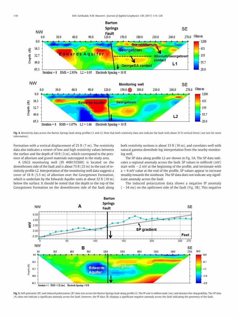
Fig. 4. Resistivity data across the Barton Springs fault along profiles L1 and L2. Note that both resistivity data sets indicate the fault with about 25 ft vertical throw (see text for moreinformation).


Formation with a vertical displacement of 25 ft (7 m). The resistivitydata also indicates a veneer of low and high resistivity values betweenthe surface and the depth of 10 ft (3 m), which correspond to the pres-ence of alluvium and gravel materials outcropped in the study area.

A USGS monitoring well (ID #08155500) is located on thedownthrown side of the fault and is about 75 ft (23m) to the east of re-sistivity profile L2. Interpretation of themonitoringwell data suggests acover of 18 ft (5.5 m) of alluvium over the Georgetown Formation,which is underlain by the Edwards Aquifer units at about 32 ft (10 m)below the surface. It should be noted that the depth to the top of theGeorgetown Formation on the downthrown side of the fault along

Fig. 5. Self-potential (SP) and induced polarization (IP) data sets across the Barton Springs fault(A) does not indicate a significant anomaly across the fault; however, the IP data (B) displays

both resistivity sections is about 33 ft (10 m), and correlates well withnatural gamma downhole log interpretation from the nearby monitor-ing well.

The SP data along profile L2 are shown in Fig. 5A. The SP data indi-cates a regional anomaly across the fault. SP values in millivolt (mV)start with −2 mV at the beginning of the profile, and terminate witha +4 mV value at the end of the profile. SP values appear to increasesteadily towards the southeast. The SP data does not indicate any signif-icant anomaly across the fault.

The induced polarization data shows a negative IP anomaly(−34 ms) on the upthrown side of the fault (Fig. 5B). This negative

along profile L2. The IP unit ismilliseconds (ms) and denotes the chargeability. The SP dataa significant negative anomaly across the fault indicating the geometry of the fault.

Fig. 6. Seismic refraction data across the Barton Springs fault along profile L2. The seismic data indicates the Georgetown Formation overlies the Edwards Aquifer unit on an uneven paleo-surface on either side of the fault. The fault throw on the seismic section is about 20 ft (6 m).


anomaly loses its magnitude across the fault but it still displays neg-ative values in the downthrown sidewithin the Edwards Aquifer unit(Fig. 5B). The source causing the negative IP anomaly is not known.

The seismic refraction tomography data across the fault is givenin Fig. 6, which shows the Georgetown Formation has an averageseismic velocity of 10,000 ft/s (3000 m/s), which is overlain with alow velocity layer of 1000 to 5000 ft/s (300 to 1500 m/s). The Ed-wards Aquifer unit underlies the Georgetown Formation, and hasan average velocity of 15,000 ft/s (4500 m/s). The Georgetown For-mation overlies the Edwards Aquifer unit on an uneven paleo-surface on either side of the fault. The fault throw on the seismic sec-tion is about 20 ft (6 m).

Fig. 7. Approximate transposition of SP anomalies onto an aerial photo of the Barton Springs swwhich could indicate a common source, such as the ground water flowing across the fault via t

4.2. Self-potential results along the banks of Barton Springs pool and insouth Zilker Park

Two SP profiles, crossing the Barton Springs fault, were run on thesouth and north banks of the swimming pool in order to locate karsticfeatures. Resultswere published in Saribudak et al., 2013,which indicat-ed a high SP anomaly located on the southbankof the swimmingpool. Asimilar anomaly along the northern bank, across from the pool, was alsoobserved. Both SP profiles also indicate a low SP anomaly in the near vi-cinity of the Barton Springs fault (see Fig. 14 in Saribudak et al., 2013).

Locations of both high and low SP anomalies aremarked on an aerialmap of the Barton Springs pool as shown in Fig. 7. It is important to note

imming pool. Note that the high SP anomalies (A and B) face each other across the fault,he same conduit.


that the SP anomaly A aligns itself in approximately the same directionas the ground water flows into the swimming pool.

4.3. Geophysical results from south Zilker Park

Because of the presence of the high SP anomaly on the southernbank of the pool, additional geophysical surveys were conducted insouth Zilker Park in order to investigate the anomaly's origin. Locationsof the geophysical profiles are shown in Fig. 3.

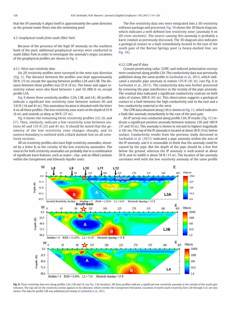
4.3.1. West-east resistivity dataSix 2D resistivity profiles were surveyed in the west-east direction

(Fig. 3). The distance between the profiles was kept approximately50 ft (15 m) except the spacing between profiles L3A and L3B. The dis-tance between those profiles was 25 ft (8 m). The lower and upper re-sistivity values were also fixed between 1 and 10, 000 Ω·m, exceptprofile L3A.

Fig. 8 shows three resistivity profiles (L3A, L3B, and L4). All profilesindicate a significant low resistivity zone between stations 45 and135 ft (14 and 41m). This anomalous location is denotedwith the letterA on all three profiles. The low resistivity zone starts at the depth of 25 ft(8 m) and extends as deep as 90 ft (27 m).

Fig. 9 shows the remaining three resistivity profiles (L5, L6, andL7). They, similarly, indicate a low resistivity zone between sta-tions 45 and 135 ft (23 and 41 m). It should be noted that the ge-ometry of the low resistivity zone changes sharply, and itseastern boundary is outlined with a black dashed-line on all resis-tivity sections.

All six resistivity profiles also have high resistivity anomalies, denot-ed by a letter B, in the vicinity of the low resistivity anomalies. Thesources for both resistivity anomalies are probably due to a combinationof significant karst features, such as water-, clay- and air-filled conduitswithin the Georgetown and Edwards Aquifer units.

Fig. 8. Three resistivity data sets along profiles L3A, L3B and L4 (see Fig. 3 for location). All thentrance. The top soil on the resistivity section appears to be alluvium, which overlies the Geshown. The data for profile L3B was published previously in Saribudak et al., 2013.

The five resistivity data sets were integrated into a 3D resistivitysoftware package and processed. Fig. 10 shows the 3D block diagram,which indicates a well-defined low resistivity zone (anomaly A on2D cross-sections). The source causing this anomaly is probably akarst conduit as previously discussed. The 3D diagram also indicatesa geological contact or a fault immediately located to the east of thesouth gate of the Barton Springs pool (a heavy-dashed line, seeFig. 10).

4.3.2. GPR and IP dataGround penetrating radar (GPR) and induced polarization surveys

were conducted along profile L3A. The conductivity datawas previouslypublished along the same profile in Saribudak et al., 2013, which indi-cated a metallic pipe anomaly at station 135 ft (41 m) (see Fig. 6 inSaribudak et al., 2013). The conductivity data was further processedby removing the pipe interference in the vicinity of the pipe anomaly.The residual data indicated a significant conductivity contrast on bothsides of station 200 ft (61 m). This observation suggests a geologicalcontact or a fault between the high conductivity unit to the east and alow conductivity material to the west.

TheGPR data obtained along L3A is shown in Fig. 11, which indicatesa fault-like anomaly immediately to the east of the pool gate.

An IP survey was conducted along profile L3A. IP results (Fig. 12) in-dicate a significant positive anomaly between stations 120 and 180 ft(37 and 55m). This anomaly is shown in red and its highest magnitudeis 181ms. The top of the IP anomaly is located at about 30 ft (9m)belowsurface. Conductivity results from the previous study discussed inSaribudak et al. (2013) indicated a pipe anomaly within the area ofthe IP anomaly, and it is reasonable to think that the anomaly could becaused by the pipe. But the depth of the pipe should be a few feetbelow the ground, whereas the IP anomaly is well-seated at about30 ft, and its width is about 50 ft (15 m). The location of the anomalycorrelates well with the low resistivity anomaly of the same profile

ree profiles indicate a significant low resistivity anomaly in the vicinity of the south gateorgetown Formation. Locations of north-south resistivity lines (L8 through L12) are also

Fig. 9. Three resistivity data sets along profiles L5, L6 and L7. All three profiles indicate a significant low resistivity anomaly in the vicinity of the south gate entrance. See text forexplanation. Resistivity profile L7 was published previously in Saribudak et al., 2013.


(see L3A in Fig. 8). Thus the source of the IP anomaly should be geologicin origin.

It should be noted that the GPR data does not indicate any metallicpipe anomaly observed in the conductivity data (see Fig. 11). The E-Wresistivity profiles shown in Figs. 8 and 9 did not indicate the presenceof any pipe-effect on either the raw or processed data. This observationsuggests that the pipe effect on the resistivity and IP data was minimal.

4.3.3. Self-potential dataSelf-potential data was collected along profiles L3A and L3B, as

displayed in Fig. 13. Both SP data sets indicate a similar, high SP anomaly

Fig. 10. A pseudo-3-D resistivity block diagram constructed using the 2-D east-westresistivity profiles of Figs. 8 and 9. Note that the 3-D diagram indicates a well-definedlow conductivity zone in the direction of the Barton Springs swimming pool near thesouth gate. The 3-D data also suggest a fault located immediately to the east of the southgate, which is indicated by a star symbol.

between stations zero and 200 ft (0 and 61m). These surveyswere donetwice in different seasons (winter and summer), using the same basestation, and identical data were obtained. These data sets were previ-ously published in Saribudak et al. (2013).

These SP anomalies obtained here are quite similar to those publishedby Schiavane and Quarto (1984). Their SP anomaly was seen over a freshwater aquifer contact between geological units with differing couplingcoefficients. The SP anomalies obtained in this study could also be dueto a geological contact (possibly a fault) involving a karst conduit.

4.3.4. Seismic refraction dataThe seismic data was collected along two profiles (L3A and L5).

These profiles were separated by 100 ft and surveyed to the south ofthe Barton Springs swimming pool (see Fig. 3 for location).

Fig. 11. GPR data along profile L3A. Note the downward bending of the layers at station105, which is located to the immediate east of the south gate. The source causing thiscould be either an erosional feature or an existing fault. The red arrows indicate theapproximate boundaries of the south gate to the Barton Springs swimming pool.

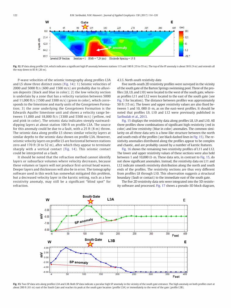
Fig. 12. IP data along profile L3A, which indicates a significant high IP anomaly between stations 115 and 180 ft (35 to 55m). The top of the IP anomaly is about 30 ft (9m) and extends allthe way down to 85 ft (26 m).


P-wave velocities of the seismic tomography along profiles L3Aand L5 show three distinct zones (Fig. 14): 1) Seismic velocities of2000 and 5000 ft/s (600 and 1500 m/s) are probably due to alluvi-um deposits (black and blue in color); 2) the low velocity sectionis underlain by a zone that has a velocity variation between 5000and 11,000 ft/s (1500 and 3300 m/s) (green in color), which corre-sponds to the limestone and marly units of the Georgetown Forma-tion; 3) the zone underlying the Georgetown Formation is theEdwards Aquifer limestone unit and shows a velocity range be-tween 11,000 and 18,000 ft/s (3300 and 5500 m/s) (yellow, redand pink in color). The seismic data indicates steeply eastward-dipping layers at about station 100 ft on profile L3A. The sourcefor this anomaly could be due to a fault, with a 25 ft (8 m) throw.The seismic data along profile L5 shows similar velocity layers atsimilar depths to the seismic data shown on profile L3A. However,seismic velocity layers on profile L5 are horizontal between stationszero and 170 ft (0 to 52 m), after which they appear to terminatesharply with a vertical contact (Fig. 14). This seismic contactcould be interpreted as a fault.

It should be noted that the refraction method cannot identifylayers or subsurface volumes where velocity decreases, becausethese volumes or layers will not produce first-arrival head waves.Deeper layers and thicknesses will also be in error. The tomographysoftware used in this work has somewhat mitigated this problem,but a decreased velocity layer in the karstic setting, such as a lowresistivity anomaly, may still be a significant “blind spot” forrefraction.

Fig. 13. Two SP data sets along profiles L3A and L3B. Both SP data indicate a peculiar high SP anabout 200 ft (61 m) east of the South Gate and reaches its peak at the south gate location (pro

4.3.5. North-south resistivity dataFive north-south 2D resistivity profiles were surveyed in the vicinity

of the south gate of the Barton Springs swimmingpool. Three of the pro-files (L8, L9, and L10)were located to thewest of the south gate, where-as profiles L11 and L12 were located to the east of the south gate (seeFig. 3 for location). The distance between profiles was approximately50 ft (15 m). The lower and upper resistivity values are also fixed be-tween 1 and 10, 000 Ω·m, as on the east-west profiles. It should benoted that profiles L9, L10 and L12 were previously published inSaribudak et al., 2013.

Fig. 15 displays the resistivity data along profiles L8, L9 and L10. Allthree profiles show combinations of significant high resistivity (red incolor) and low resistivity (blue in color) anomalies. The common simi-larity on all three data sets is a bow-like structure between the northand south ends of the profiles (see black dashed lines in Fig. 15). The re-sistivity anomalies distributed along the profiles appear to be complexand chaotic, and are probably caused by a number of karstic features.

Fig. 16 shows the remaining two resistivity profiles of L11 and L12.The lower and upper resistivity values of these sections were also heldbetween 1 and 10,000 Ω·m. These data sets, in contrast to Fig. 15, donot show significant anomalies. Instead, the resistivity data on L11 andL12 indicate smooth resistivity distribution along the north and southends of the profiles. The resistivity sections are thus very differentfrom profiles L8 through L10. This observation suggests a structuralboundary (fault or contact) to the immediate east of the south gate.

The five 2D resistivity data sets were integrated into the 3D resistiv-ity software and processed. Fig. 17 shows a pseudo-3D block diagram,

omaly in the vicinity of the south gate entrance. The high anomaly on both profiles start atfile L3A) or immediately to the west of the gate (profile L3B).

Fig. 14. Seismic refraction data sets along profiles L3A and L5. Profile L3A indicates a fault-like pattern at station 100 ft (30 m). However, profile L5 does not show a similar fault-likeanomaly as profile L3A. Instead it displays a sharp contact at about 200 ft (61 m) at the depth of 30 ft (9 m), which could be due to a fault.


which indicates a well-defined low resistivity zone at the northern endof the profiles L8 through L12. The source causing this anomaly could bedue to a karst conduit.

It should be noted that an attempt was made to combine the 2Deast-west and north-south resistivity profiles in a single 3-D file andrun through the EarthImager 3D software. However, this goal was notpossible with the commercially available 3D software.

5. Discussion and conclusions

The results of the geophysical surveys across the known location ofthe Barton Springs fault confirm the presence of the fault. Two resistiv-ity profiles indicate the fault and its 25 ft (8m) vertical throw. The seis-mic refraction data defines an irregular paleo-surface between theGeorgetown and Edwards Aquifer in the vicinity of the fault. The faultthrow displayed by the seismic refraction data is about 20 ft (6 m).The soil thickness overlying the Georgetown Formation is depicted asabout 18 ft, which is similar to the monitoring well and the resistivitydata. The IP data further confirms the location of the fault. The IP anom-aly across the fault, however, is negative in polarity. The lowest magni-tude of the IP anomaly corresponds to the upthrown side, where theEdwards Aquifer limestone unit is located. The SP data displays a

fault-like anomaly across the Barton Springs fault. There is no significanthigh SP anomaly across the fault that would indicate karstic features.Thus the absence of the high SP anomaly suggests that the groundwater flow across the fault is insignificant.

The offset of the Barton Springs fault, based on the geological obser-vations, is between 20 and 70 ft (6 to 21m). However, geophysical dataindicate the fault throw between 20 and 25 ft (6 and 8 m).

The SP data obtained from the south bank of the Barton Springs poolindicates a significant high and wide SP anomaly (Saribudak et al.,2013). The source for this anomaly can be attributed to the groundwater flowwithin the conduits of Georgetown and/or Edwards Aquiferunits.

Six west-east resistivity profiles, which are in the south ZilkerPark, indicate significant low and high resistivity anomalies betweenthe west starting points of the resistivity profiles and the south gatelocated along the southern fence of the pool. The geometry and dis-tribution of these anomalies differ sharply from profile to profile.But they all start at a depth of 25 ft and appear to continue as deepas 98 ft (23 to 30 m). The 3D west-east resistivity diagram indicatesa well-defined low resistivity zone (a conduit) and a structuralboundary (a fault or geological contact) to the immediate east ofthe south gate.

Fig. 15. Resistivity data along profiles L8, L9, and L10 in the north-south direction. All three profiles show combinations of significant low resistivity (blue) and high resistivity (red)anomalies. The common similarity on all three data sets is a bow-like structure between the north and south ends of the profiles. Locations of east-west resistivity lines (L3A, L3B, L4,L5 and L7) are shown. Resistivity profile L10 was published previously in Saribudak et al., 2013.


One IP profile, which was collected along profile 3A, indicates a highIP anomaly, which corresponds to the location of the low resistivityanomaly. The magnitude of this anomaly is significantly high, 181 ms,and its cause is not known.

Two seismic refraction data sets along profiles L3A and L5 con-tain geological information with regard to the contacts of the geo-logical units in the study area. According to the seismic refraction

Fig. 16. Two resistivity data sets along profiles L11 and L12 in the north-south direction. Thesobservation suggests a structural boundary (fault or a geological contact) to the east of the sou

tomography data, both profiles indicate an average of 10 to 20 ft(3 to 6 m) of alluvium which is underlain by the Georgetown For-mation. The Georgetown Formation has a thickness of about 20 ft,and overlies the Edwards Aquifer units. Thus, the thickness of thegeological units correlates well with the monitoring data and theresistivity data from the west of the study area over the BartonSprings fault.

e data sets, in contrast to those shown in Fig. 15, do not show significant anomalies. Thisth gate. Resistivity profile L11 was published previously in Saribudak et al., 2013.

Fig. 17. A pseudo 3-D resistivity block diagram constructed using the 2-D north-southresistivity profiles of Figs. 15 and 16. Note that the 3-D diagram indicates a well-definedlow conductivity zone in the direction of the Barton Springs swimming pool in thevicinity of the south gate entrance, which is marked by the star symbol.


Three of the five north-south resistivity profiles in front of the southgate indicate significant low resistivity anomalies along the lengthof theprofiles. There are also high resistivity anomalies associated with thelow resistivity anomalies. It should be noted that three resistivity pro-files indicate a bow-like geometry. But the remaining two profiles,which are located to the east of the south gate, do not indicate any sig-nificant anomaly. The 3Dnorth-south resistivity block indicates a signif-icant low resistivity anomaly (a conduit) in the vicinity of the southgate.

In summary, these geophysical findings indicate significant anoma-lies to the south of the Barton Springs pool. Themajority of these anom-alies indicates a fault-like pattern in front of the south gate entrance. Thelocation of geophysical anomalies obtained from surveys performedacross the Barton Springs fault and from the area situated to the south

Fig. 18. Map showing the locations of the geophysical anomalies and the elevation values of tswimming pool. Geophysical anomalies include a fault trending in the NW-SE direction from t

of the swimming pool are shown in Fig. 18. Those anomalies revealsignificant information on the Barton Springs fault. In addition,geophysical results suggest the presence of a large conduit and afault in the southern part of the Barton Springs pool. The ground-water flow-path to the Main Springs could follow the locations ofthose resistivity and SP anomalies along this newly discoveredfault instead of the Barton Springs fault, as previously thought.This fault appears to cut the Barton Springs fault obliquely and itswestern side is upthrown.

In order to support the existence of the new fault with the geo-logical data, elevations of the Georgetown Formation in thedownthrown side of the Barton Springs fault were obtained andare shown in Fig. 18. The average elevation of the GeorgetownFormation on the northern side of the swimming pool is 423 ft(121 m) above sea level for seven boring locations (David Johns ofCity of Austin, personal communication, 2015). In the south partof the swimming pool, however, the average elevation value is453 ft (138 m), and is obtained from five sources (the monitoringwell data, an outcrop, two seismic refraction studies, and aresistivity profile) (Fig. 18). A 30 ft (9 m) elevation difference is ob-served at the downthrown side along the Barton Springs fault be-tween the north and the south areas. If there was no interveningfault, the averaged elevation values of the Georgetown Formationshould have similar values on the downward side of the BartonSprings fault across the swimming pool. Instead, the 30 ft (9 m)difference in elevation values of the Georgetown Formationsupports the existence of the fault suggested by the geophysicaldata.

The newly identified fault in south Zilker Park is antithetical tothe Barton Springs fault. Antithetic faults have been widely ob-served in the Balcones Fault Zone, and they typically form afterstress release associated with the formation of a synthetic faultand subsequent perpendicular rotation of stress fields (Kulanderet al., 1979).

Acknowledgments

We thank Alf Hawkins and Justin Camp for their help during thefieldwork and their enthusiastic support for this project. Our apprecia-tions go to Siegfried Rohdewald of Rayfract Software and Brad Carr fortheir help in processing the seismic refraction data and the induced

he Georgetown Formation across the northern and southern parts of the Barton Springshe south in Zilker Park towards the Barton Springs fault, and a conduit along the fault.


polarization data, respectively.We appreciate Phil Carpenter's review ofthe manuscript, which helped improve its English and its flow greatly.

We also thank the following colleagues for their help in obtainingthe permission to perform the geophysical surveys at the Barton Springspool and for their eager interest: David Johns, Tom Nelson, WayneSimmons, Margaret Russell, Sylvia Pope, Nate Benedict, Laurie Dries,and George Veni.

This project was borne out of personal interest and was supportedby Environmental Geophysics Associates.

References

Ahmed, S., Carpenter, P.J., 2003. Geophysical response of filled sinkholes, soil pipes andassociated bedrock fractures in thinly mantled karst, east-central Illinois. Environ.Geol. 44, 705–716.

Atangana, J.Q.Y., Angue, M.A., Nyeck, B., Ndongue, C., Tchatat, J.T., 2015. Electrical charac-terization and mineralogical differentiation of a weathering cover in the SouthCameroon Humid Intertropical Zone using the self-potential method. J. Environ.Eng. Geophys. 20 (1), 57–70.

Bery, A.A., Saad, R., Mohamad, E.D., Jinmin, M., Azwin, L.N., Tan, N.M.A., Nordiana, M.M.,2012. Electrical resistivity and induced polarization data correlation with conductiv-ity for iron ore exploration. EJGE 17, 3223–3237.

Carpenter, P.J., 1998. Geophysical character of buried sinkholes on the oak ridge reserva-tion, Tennessee. J. Environ. Eng. Geophys. 3, 133–146.

Chen, J., Zelt, C.A., 2016. Application of frequency-dependent Traveltime tomography andfull waveform inversion to realistic near-surface seismic refraction data. J. Environ.Eng. Geophys. 21 (1), 1–12.

Connor, C.B., Sandberg, S.K., 2001. Application of Integrated Geophysical Techniques toCharacterize the Edwards Aquifer. STGS Bulletin, Texas, pp. 11–25 (March issue).

Dahlin, T., Leroux, V., Nissen, J., 2002. Measuring techniques in induced polarizationimaging. J. Appl. Geophys. 50, 279–298.

Dobecki, T., Upchurch, S., 2006. Geophysical applications to detect sinkholes and groundsubsidence. Lead. Edge 25 (3), 336–341.

Ferrill, D.A., Morris, A.P., Waiting, D.J., 2005. Structure of the Balcones Fault System andArchitecture of the Edwards and Trinity Aquifers, South-Central, Texas. A Field TripGuide for the South-Central Geological Society of America Meeting.

Freeland, R.S., 2015. Imaging the lateral roots of the orange tree using three-dimensionalGPR. J. Environ. Eng. Geophys. 20 (3), 235–244.

Freeland, R.S., Allred, B.J., Martinez, L.R., Gamble, D.L., Jones, B.R., McCoy, E.L., 2016. Perfor-mance of hybrid and single-frequency impulse GPR antennas on USGA sportinggreens. J. Environ. Eng. Geophys. 21 (2), 57–65.

Garner, L.E., Young, K.P., Rodda, P.U., Dawe, G.L., Rogers, M.A., 1976. Geologic map of theAustin area, Texas, in Garner: an aid to urban planning. Univ. Tex. Austin, Bur. Econ.Geol. scale 1 (65), 500.

Hauwert, N.M., 2009. Groundwater Flow and Recharge within the Barton Springs Seg-ment of the Edwards Aquifer, Southern Travis and Northern Hays Counties, Texas.(A Ph.D. Dissertation). The University of Texas, Austin.

Hauwert, N.M., Johns, D., Hunt, B., Beery, J., Smith, B., Sharp, J.M., 2004. Flow systems ofthe Edwards Aquifer Barton Springs Segment interpreted from tracing and associatedfield studies: from Edwards Water Resources. Central Texas, Retrospective and Pro-spective Symposium Proceedings, San Antonio, Hosted by the South Texas GeologicalSociety and Austin Geological Society (18 pp.).

Hunt, B.B., Smith, B.A., Campbell, S., Beery, J., Hauwert, N., Johns, D., 2005. Dye tracing re-charge features under high-flow conditions, Onion Creek, Barton Springs segment ofthe Edwards aquifer, Hays County, Texas. Austin Geol. Soc. Bull. 5, 70–86.

Johns, D., 2015. Continuous discharge data from Barton Springs and rainfall since 1978. In:Hauwert, N., Johns, D., Hunt, B. (Eds.), Karst and Recharge in the Barton Springs

Segment of the Edwards Aquifer: Field Trip to the City of Austin's Water QualityProtection Lands. Austin Geological Society Guidebook 35, pp. 46–49.

Kulander, B.R., Barton, C.C., Dean, S.L., 1979. The Application of Fractography to Core andOutcrop Fracture Investigations: Report Prepared for US DOE (174 pp.).

Lachhab, A., Booterbaugh, A., Beren, M., 2015. Bathymetry and sediment accumulation ofWalker Lake, PA using two GPR antennas in a new integratedmethod. J. Environ. Eng.Geophys. 20 (3), 245–255.

Lange, A.L., 1999. Geophysical studies at Kartchner Caverns State Park, Arizona. J. CaveKarst Stud. 61 (2), 68–72.

Lange, A.L., Kilty, K.T., 1991. Natural Potential Responses of Karst Systems at the GroundSurface. Proceedings of the Third Conference on Geohydrology, Ecology andMonitor-ing and Management of Ground Water in Karst Terranes: National GroundwaterAssociation pp. 179–196.

Mahler, B.J., Lynch, F.L., 1999. Muddy waters: temporal variation in sediment dischargingfrom a karst spring. J. Hydrol. 214, 165–178.

Musgrove,M., Banner, J.L., 2004. Controls on the spatial and temporal variability of vadosedripwater geochemistry: Edwards Aquifer, central Texas. Geochim. Cosmochim. Acta68 (5), 1007–1020.

Palmer, N.A., 2007. Cave Geology. Published by Cave Books.Parasnis, D.S., 1996. Principles of Applied Geophysics. fifth ed. Springer.Rose, P.R., 1972. Edwards group, surface and subsurface, Central Texas. Report of Investi-

gations 74. Bureau of Economic Geology, Austin, Texas.Rucker, D.F., Ferré, T.P.A., 2004. Automated water content reconstruction of zero-offset

borehole ground penetrating radar data using simulated annealing. J. Hydrol. 309(1–4), 1–16.

Rucker, D.F., Glaser, D.R., 2015. Standard, random and optimum Array conversions fromtwo-pole resistance data. J. Environ. Eng. Geophys. 20 (3), 207–217.

Saribudak, M., 2011. Urban geophysics: geophysical signature of Mt. Bonnell Fault and itskarstic features in Austin, Texas, Houston. Geol. Soc. Bull. (October), 49–54.

Saribudak, M., Hawkins, A., Stoker, K., 2012a. Geophysical signature of Haby CrossingFault and its implication on the Edwards Recharge Zone, Medina County, Texas.Houston Geophys. Soc. Bull. 2, 9–14.

Saribudak, M., Hunt, S., Smith, B., 2012b. Resistivity imaging and natural potential appli-cations to the Antioch Fault Zone in the Onion Creek/Barton Springs segment of theEdwards Aquifer, Buda, Texas. Gulf Coast Assoc. Geol. Soc. Trans. 62, 411–421.

Saribudak, M., Hauwert, N., Hawkins, A., 2013. Geophysical Signatures of Barton Springs(Parthenia, Zenobia and Eliza) of the Edwards Aquifer. Austin, Texas, Sinkhole Con-ference 14 Proceedings, Carbonite and EvaporitesSpringer (ISSN 0891-2556).

Schiavane, D., Quarto, R., 1984. Self-potential prospecting in the study of water move-ments. Geoexploration 22, 47–58.

Small, T.A., Hanson, J.A., Hauwert, N.M., 1996. Geologic framework and hydrogeologiccharacteristics of the Edwards Aquifer outcrop (Barton Springs Segment), northeast-ern Hays and southwestern Travis Counties, Texas. U.S. Geological Survey WaterResources Investigations, pp. 96–4306 (15 pp. Prepared in cooperation with theBS/EACD and TWDB).

Telford, W.M., Geldart, L.P., Sheriff, R.E., 1990. Applied Geophysics. second ed. CambridgeUniversity Press.

Thuesen, K., 2013. Restoring land and managing karst to protect water quality andquantity at Barton Springs, Austin, Texas. In: Land, L., Doctor, D., Stephenson, J.(Eds.), Sinkholes and the Engineering and Environmental Impacts of Karst. Pro-ceedings of the Thirteenth Multidisciplinary Conference. National Cave andKarst Research Institute, Carlsbad, New Mexico.

Vichabian, Y., Morgan, F.D., 2002. Self potentials in cave detection. Lead. Edge 23,866–871.

Xianxin, S., Kai, W., 2011. Induced polarization method applied for groundwater resourceexploration, water resource and environmental protection (ISWREP). Int. Symp. 1,365–368.

http://refhub.elsevier.com/S0926-9851(17)30014-9/rf0005





































































































journal of applied geophysics geophysics_jog_2017.pdfa environmental geophysics associates, austin,...

Documents