journal of applied ecology using camera trapping and ... camera trapping and...camera trap studies...

Using camera trapping and hierarchical occupancy

modelling to evaluate the spatial ecology of an African

mammal community

Lindsey N. Rich1,2*, David A.W. Miller3, Hugh S. Robinson4, J. Weldon McNutt2 and

Marcella J. Kelly1

1Department of Fish and Wildlife Conservation, Virginia Tech, 318 Cheatham Hall, Blacksburg, VA, USA; 2Botswana

Predator Conservation Trust, Maun, Botswana; 3Department of Ecosystem Science and Management, Penn State

University, 411 Forest Resources Building, University Park, PA, USA; and 4Panthera and College of Forestry and

Conservation, University of Montana, Missoula, MT, USA

Summary

1. Emerging conservation paradigms have shifted from single to multi-species approaches

focused on sustaining biodiversity. Multi-species hierarchical occupancy modelling provides a

method for assessing biodiversity while accounting for multiple sources of uncertainty.

2. We analysed camera trapping data with multi-species models using a Bayesian approach

to estimate the distributions of a terrestrial mammal community in northern Botswana and

evaluate community, group, and species-specific responses to human disturbance and environ-

mental variables. Groupings were based on two life-history traits: body size (small, medium,

large and extra-large) and diet (carnivore, omnivore and herbivore).

3. We photographed 44 species of mammals over 6607 trap nights. Camera station-specific

estimates of species richness ranged from 8 to 27 unique species, and species had a mean

occurrence probability of 0�32 (95% credible interval = 0�21–0�45). At the community level,

our model revealed species richness was generally greatest in floodplains and grasslands and

with increasing distances into protected wildlife areas.

4. Variation among species’ responses was explained in part by our species groupings. The posi-

tive influence of protected areas was strongest for extra-large species and herbivores, while med-

ium-sized species actually increased in the non-protected areas. The positive effect of grassland/

floodplain cover, alternatively, was strongest for large species and carnivores and weakest for

small species and herbivores, suggesting herbivore diversity is promoted by habitat heterogeneity.

5. Synthesis and applications. Our results highlight the importance of protected areas and

grasslands in maintaining biodiversity in southern Africa. We demonstrate the utility of hier-

archical Bayesian models for assessing community, group and individual species’ responses to

anthropogenic and environmental variables. This framework can be used to map areas of

high conservation value and predict impacts of land-use change. Our approach is particularly

applicable to the growing number of camera trap studies world-wide, and we suggest broader

application globally will likely result in reduced costs, improved efficiency and increased

knowledge of wildlife communities.

Key-words: biodiversity, body size, camera trap, diet, grasslands, hierarchical Bayesian mod-

els, human disturbance, multi-species modelling, protected areas, species richness

Introduction

Prioritizing conservation actions, quantifying the impacts

of management decisions and designating protected areas

are just a few of the challenging tasks faced by wildlife

managers and conservationists. To address these tasks,

surrogate species are often used (Carroll, Noss & Paquet

2001; Epps et al. 2011) such that by focusing on the

requirements of the surrogate, the needs of an entire

community are addressed (Lambeck 1997). This concept,

however, is widely debated given that actions aimed at*Correspondence author. E-mail: [email protected]

© 2016 The Authors. Journal of Applied Ecology © 2016 British Ecological Society

Journal of Applied Ecology 2016 doi: 10.1111/1365-2664.12650

conserving a single species have positive and negative

effects on a wealth of other non-target species (Simberloff

1998; Wiens et al. 2008). As a result, emerging conserva-

tion and management paradigms favour multi-species vs.

single species approaches where the objective is sustaining

biodiversity and ecosystem functions (Yoccoz, Nichols &

Boulinier 2001; Balmford et al. 2005).

Multi-species hierarchical occupancy models (Dorazio

& Royle 2005), a recent advancement in community mod-

elling, can be used to evaluate the spatial ecology of wild-

life communities. As occupancy models (MacKenzie et al.

2002), they account for imperfect detection using tempo-

rally or spatially replicated data collected in a time period

during which populations are assumed to be geographi-

cally closed. As hierarchical models, they integrate data

across species, permitting composite analyses of communi-

ties, species groups and individual species (Russell et al.

2009; Zipkin, DeWan & Royle 2009). Sharing data across

species leads to increased precision in estimates of species

richness and species-specific occupancy, particularly for

rare and elusive species (Zipkin et al. 2010). Multi-species

hierarchical models can also be parameterized with vari-

ables hypothesized to influence the distributions of wild-

life, allowing evaluation of how these variables affect

wildlife communities, groups of species or a species of

concern (Russell et al. 2009).

The spatial ecology of wildlife is often shaped by

human disturbance. Increasing human populations and

the corresponding demand for land has resulted in land-

use change, fragmentation and infrastructure development

being some of the greatest threats to biodiversity (Alke-

made et al. 2009). One of the most prevalent forms of

land-use change is conversion of wildlands to agriculture.

Agricultural expansion has resulted in losses of 20–50%of forested land and 25% of grasslands globally (DeFries,

Foley & Asner 2004). To combat the loss of wildlands

and associated biodiversity, 12�7% of the Earth’s land

area has been designated as protected (Bertzky et al.

2012). The success of conserving biodiversity in these pro-

tected areas, however, is mixed (Western, Russell & Cut-

hill 2009; Craigie et al. 2010; Kiffner, Stoner & Caro

2013). In Kenya, for example, wildlife has declined at sim-

ilar rates inside and outside of protected areas (Western,

Russell & Cuthill 2009), whereas in Tanzania, species

within protected areas fare better (Stoner et al. 2007).

Land-use change may also lead to construction of artifi-

cial barriers such as roads and fences which can alter ani-

mal movements and fragment ecosystems (Forman &

Alexander 1998; Hayward & Kerley 2009). The impacts

of roads on wildlife vary widely, with increased human

and vehicle activity often leading to increases in road

mortality, edge effects and both legal and illegal hunting

pressure (Forman & Alexander 1998). The impact of

fences, in contrast, depends on the type of fence and pur-

pose (Hayward & Kerley 2009). Fences can minimize

threats from humans and domestic animals but if erected

with little regard to wildlife movements, the result can be

mass mortality of migrating ungulates (Hayward & Kerley

2009).

The spatial ecology of wildlife is also shaped by envi-

ronmental features such as access to water, food availabil-

ity and vegetation cover. For example, occupancy of

mammals often declines with increasing distance to per-

manent water (Pettorelli et al. 2010; Epps et al. 2011;

Schuette et al. 2013). Mesic habitats such as seasonal

floodplains, however, tend to be characterized by rela-

tively tall, less nutritious grass species (Hopcraft et al.

2012), which could result in grazing species preferring

areas further from permanent water. The influence of veg-

etation cover, alternatively, is likely to be species specific

(Estes 1991). Within the African carnivore guild, for

example, black-backed jackals Canis mesomelas often

avoid floodplains and grasslands (Kaunda 2001), whereas

servals Leptailurus serval prefer these land covers (Pet-

torelli et al. 2010; Schuette et al. 2013).

A species’ response to ecological variables may also be

influenced by their life-history traits. Theory suggests, for

example, that larger-bodied species in trophic groups at

the top of the food chain (e.g. large carnivores) are more

likely to decline than lower trophic guild species under

similar conditions (Gaston & Blackburn 1996; Davies,

Margules & Lawrence 2000). Life-history characteristics

of species at high trophic levels, including low population

densities, high food requirements and large home ranges,

make them particularly vulnerable to persecution and

fluctuating environments (Gard 1984; Ripple et al. 2014).

Large-bodied animals are also targeted by trophy hunters

(Packer et al. 2009) and bushmeat hunters (Fa, Ryan &

Bell 2005). Consequently, we would expect large-bodied

species near the top of the food chain to show greater

sensitivity to anthropogenic and environmental changes.

In this study, we explore the utility of camera trap sur-

veys and multi-species hierarchical models to inform bio-

diversity management. We applied our multi-species

approach to a community of mammals in the Okavango

Delta, Botswana – a World Heritage Site that is home to

abundant wildlife including some of Africa’s most endan-

gered mammals. Better understanding of the spatial ecol-

ogy of the mammal community will allow managers to

more fully balance gains against losses when managing

the diversity of wildlife (Western, Russell & Cuthill 2009;

Zipkin, DeWan & Royle 2009). Additionally, our research

was motivated by the lack of broad-scale wildlife commu-

nity studies. Community-level studies generally focus on a

particular guild of species such as carnivores (Pettorelli

et al. 2010; Schuette et al. 2013) or ungulates (Stoner

et al. 2007; Western, Russell & Cuthill 2009; Kiffner,

Stoner & Caro 2013). Our study is among the first to

evaluate the distributions of all terrestrial mammals

>0�5 kg, excluding rodents.

Our specific objectives were to quantify species richness,

evaluate species’ distributions and elucidate community,

group, and species-specific responses to human disturbance

and environmental variables. We hypothesized (i) species

© 2016 The Authors. Journal of Applied Ecology © 2016 British Ecological Society, Journal of Applied Ecology

2 L. N. Rich et al.

richness, group richness and species-specific occupancy

would be inversely related to human disturbance with

large-bodied wildlife and carnivores expected to show the

strongest relationships (Epps et al. 2011; Hopcraft et al.

2012; Schuette et al. 2013) and (ii) environmental condi-

tions related to occupancy, in comparison with human dis-

turbance, would be unique to each species and have

weaker community and group-level effects. Our research

aims to provide a better understanding of how environ-

mental features and anthropogenic pressures are impacting

species’ distributions in southern Africa. Additionally, our

analysis framework is applicable to the growing number of

camera trap studies world-wide and could be applied to

various land-use-related activities including mapping areas

of high conservation value, predicting the effects of human

development and providing guidance for management

strategies aimed at sustaining biodiversity.

Materials and methods

STUDY AREA

Our study was carried out in Ngamiland District of northern

Botswana, where the Okavango Delta and the northern reaches

of the Kalahari Desert are located. The area (c. 550 km2; 19˚31ʹS23˚37ʹE) included a mixture of floodplains/grasslands, acacia

woodland savannas, mopane Colophospermum mopane shrub and

woodlands, and mixed shrublands. Our study site included the

eastern section of Moremi Game Reserve, wildlife management

areas NG33/34 and part of the livestock grazing areas of Shorobe

(Fig. 1). Wildlife was fully protected within Moremi Game

Reserve and partially protected within the wildlife management

areas under a policy known as community-based natural resource

management (Mbaiwa, Stronza & Kreuter 2011). Both areas were

primarily used for photographic tourism. Moremi, however, was

open to self-drive tourists and safari companies, whereas the

wildlife management areas were only accessible to Sankuyo

community members and safari companies with leases in the

area. Consequently, the game reserve had higher human activity

(�x = 6 vehicles per day per camera station) than the wildlife man-

agement areas (�x = 2 vehicles per day per camera station). The

wildlife management areas were separated from adjacent livestock

grazing areas by an extensive 1�3-m high cable veterinary fence

that was erected to prevent the transmission of foot-and-mouth

disease from Cape buffalo Syncerus caffer to cattle (Keene-Young

1999). Carnivores and other wildlife species, however, commonly

pass through the fence (Keene-Young 1999). Wildlife within the

management and livestock areas could be legally killed when the

animal posed a threat to human life or property (Republic of

Botswana Conservation and National Parks Act 2001).

Fig. 1. Our study area including the eastern section of Moremi Game Reserve, wildlife management areas NG33/34 and livestock graz-

ing areas in Shorobe, Botswana.


Evaluating spatial ecology of wildlife 3

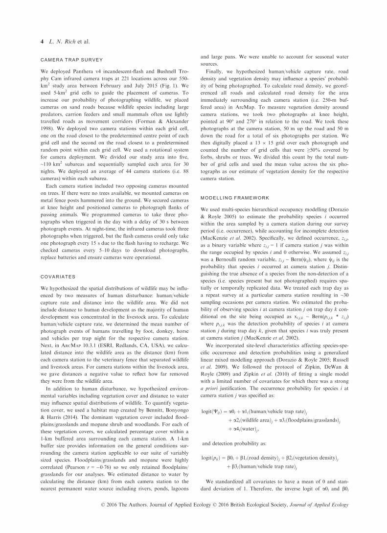
CAMERA TRAP SURVEY

We deployed Panthera v4 incandescent-flash and Bushnell Tro-

phy Cam infrared camera traps at 221 locations across our 550-

km2 study area between February and July 2015 (Fig. 1). We

used 5-km2 grid cells to guide the placement of cameras. To

increase our probability of photographing wildlife, we placed

cameras on sand roads because wildlife species including large

predators, carrion feeders and small mammals often use lightly

travelled roads as movement corridors (Forman & Alexander

1998). We deployed two camera stations within each grid cell,

one on the road closest to the predetermined centre point of each

grid cell and the second on the road closest to a predetermined

random point within each grid cell. We used a rotational system

for camera deployment. We divided our study area into five,

~110 km2 subareas and sequentially sampled each area for 30

nights. We deployed an average of 44 camera stations (i.e. 88

cameras) within each subarea.

Each camera station included two opposing cameras mounted

on trees. If there were no trees available, we mounted cameras on

metal fence posts hammered into the ground. We secured cameras

at knee height and positioned cameras to photograph flanks of

passing animals. We programmed cameras to take three pho-

tographs when triggered in the day with a delay of 30 s between

photograph events. At night-time, the infrared cameras took three

photographs when triggered, but the flash cameras could only take

one photograph every 15 s due to the flash having to recharge. We

checked cameras every 5–10 days to download photographs,

replace batteries and ensure cameras were operational.

COVARIATES

We hypothesized the spatial distributions of wildlife may be influ-

enced by two measures of human disturbance: human/vehicle

capture rate and distance into the wildlife area. We did not

include distance to human development as the majority of human

development was concentrated in the livestock area. To calculate

human/vehicle capture rate, we determined the mean number of

photograph events of humans travelling by foot, donkey, horse

and vehicles per trap night for the respective camera station.

Next, in ARCMAP 10.3.1 (ESRI, Redlands, CA, USA), we calcu-

lated distance into the wildlife area as the distance (km) from

each camera station to the veterinary fence that separated wildlife

and livestock areas. For camera stations within the livestock area,

we gave distances a negative value to reflect how far removed

they were from the wildlife area.

In addition to human disturbance, we hypothesized environ-

mental variables including vegetation cover and distance to water

may influence spatial distributions of wildlife. To quantify vegeta-

tion cover, we used a habitat map created by Bennitt, Bonyongo

& Harris (2014). The dominant vegetation cover included flood-

plains/grasslands and mopane shrub and woodlands. For each of

these vegetation covers, we calculated percentage cover within a

1-km buffered area surrounding each camera station. A 1-km

buffer size provides information on the general conditions sur-

rounding the camera station applicable to our suite of variably

sized species. Floodplains/grasslands and mopane were highly

correlated (Pearson r = �0�76) so we only retained floodplains/

grasslands for our analyses. We estimated distance to water by

calculating the distance (km) from each camera station to the

nearest permanent water source including rivers, ponds, lagoons

and large pans. We were unable to account for seasonal water

sources.

Finally, we hypothesized human/vehicle capture rate, road

density and vegetation density may influence a species’ probabil-

ity of being photographed. To calculate road density, we georef-

erenced all roads and calculated road density for the area

immediately surrounding each camera station (i.e. 250-m buf-

fered area) in ArcMap. To measure vegetation density around

camera stations, we took two photographs at knee height,

pointed at 90° and 270° in relation to the road. We took these

photographs at the camera station, 50 m up the road and 50 m

down the road for a total of six photographs per station. We

then digitally placed a 13 9 15 grid over each photograph and

counted the number of grid cells that were ≥50% covered by

forbs, shrubs or trees. We divided this count by the total num-

ber of grid cells and used the mean value across the six pho-

tographs as our estimate of vegetation density for the respective

camera station.

MODELLING FRAMEWORK

We used multi-species hierarchical occupancy modelling (Dorazio

& Royle 2005) to estimate the probability species i occurred

within the area sampled by a camera station during our survey

period (i.e. occurrence), while accounting for incomplete detection

(MacKenzie et al. 2002). Specifically, we defined occurrence, zi,j,

as a binary variable where zi,j = 1 if camera station j was within

the range occupied by species i and 0 otherwise. We assumed zi,jwas a Bernoulli random variable, zi,j ~ Bern(wij), where wij is the

probability that species i occurred at camera station j. Distin-

guishing the true absence of a species from the non-detection of a

species (i.e. species present but not photographed) requires spa-

tially or temporally replicated data. We treated each trap day as

a repeat survey at a particular camera station resulting in ~30

sampling occasions per camera station. We estimated the proba-

bility of observing species i at camera station j on trap day k con-

ditional on the site being occupied as xi,j,k ~ Bern(pi,j,k * zi,j)

where pi,j,k was the detection probability of species i at camera

station j during trap day k, given that species i was truly present

at camera station j (MacKenzie et al. 2002).

We incorporated site-level characteristics affecting species-spe-

cific occurrence and detection probabilities using a generalized

linear mixed modelling approach (Dorazio & Royle 2005; Russell

et al. 2009). We followed the protocol of Zipkin, DeWan &

Royle (2009) and Zipkin et al. (2010) of fitting a single model

with a limited number of covariates for which there was a strong

a priori justification. The occurrence probability for species i at

camera station j was specified as:

logitðWijÞ ¼ a0i þ a1iðhuman/vehicle trap rateÞjþ a2iðwildlife areaÞj þ a3iðfloodplains/grasslandsÞjþ a4iðwaterÞj;

and detection probability as:

logitðpijÞ ¼ b0i þ b1iðroad densityÞj þ b2iðvegetation densityÞjþ b3iðhuman/vehicle trap rateÞj

We standardized all covariates to have a mean of 0 and stan-

dard deviation of 1. Therefore, the inverse logit of a0i and b0i


4 L. N. Rich et al.

are the occurrence and detection probabilities, respectively, for

species i at a camera station with average covariate values.

Remaining coefficients (a1i,.., a4i, and b1i,..,b3i) represent the

effect of a one standard deviation increase in the covariate value

for species i. A species’ abundance can significantly affect detec-

tion probabilities, often resulting in strong, positive correlations

between occupancy and detection (Royle & Nichols 2003). As a

result, we modelled among species correlation (q) between a0iand b0i by specifying the two parameters to be jointly distributed

(Dorazio & Royle 2005; K�ery & Royle 2008).

We linked species-specific models using a mixed modelling

approach. We assumed species-specific parameters were random

effects derived from a normally distributed, community-level

hyper-parameter (Zipkin et al. 2010). Hyper-parameters specify

the mean response and variation among species within the com-

munity to a covariate (K�ery & Royle 2008). Specifically, for our

community model, the a coefficients were modelled as ai � nor-

mal(la, r2a) where la is the community-level mean and r2

a is the

variance (Chandler et al. 2013). We also hypothesized body size

and diet may influence how a species responds to the respective

covariates. Thus, we divided species into body size groups based

on mean body mass for males and females (Estes 1991). Groups

included extra-large (≥200 kg)-, large (50–200 kg)-, medium

(20–50 kg)- and small (<20 kg)-sized species (see Appendix S1,

Supporting information). The diet groups included carnivores,

herbivores and omnivores (Estes 1991). To assess group-level

effects, we allowed a coefficients to be species-specific and gov-

erned by a group-level and community-level hyper-parameter.

For our group models, a coefficients were modelled as functions

of the community-level mean, group-level mean (body size or diet

group) and species-specific effect for the respective covariate.

We estimated posterior distributions of parameters using Mar-

kov chain Monte Carlo (MCMC) implemented in JAGS (version

3.4.0) through program R (R2Jags; Plummer 2011). We generated

three chains of 50 000 iterations after a burn-in of 10 000 and

thinned by 50. For priors, we used a uniform distribution of 0 to

1 on the real scale for a0i and b0i and uniform from 0 to 10 for

r parameters. We used a normal prior distribution with a mean

of 0 and standard deviation of 100 on the logit-scale for the

remaining covariate effects (a1i,.., a4i and b1i,..,b3i). We assessed

convergence using the Gelman–Rubin statistic where values <1�1indicated convergence (Gelman et al. 2004).

During each iteration, the model generates a matrix of camera

station and species-specific z values (i.e. an occupancy matrix)

where as previously stated, zi,j = 1 if camera station j was within

the range occupied by species i and 0 otherwise. To estimate

species richness at camera station j, we summed the number of

estimated species (i.e. instances where zi = 1 for camera station j)

during iteration x. We then repeated this process for each of the

50 000 iterations and used these values to generate a probability

distribution representing camera station-specific species richness

(Zipkin et al. 2010). We calculated group-level richness similarly,

the only difference being that we restricted the estimate to species

belonging to the respective group. As an example, the complete

specification for the diet group model and how we calculated

species and group richness is presented in Appendix S2.

Results

We recorded 8668 detections of 44 species of mammals

during our 6607 trap nights. Body size groups included 12

small, 11 medium, 11 large and 10 extra-large species

(Appendix S1). Diet groups included 21 carnivores, 18

herbivores and 5 omnivores (Appendix S1). Brown hyae-

nas Hyaena brunnea (n = 3) and cheetahs Acinonyx juba-

tus (n = 3) were photographed least often, while African

elephants Loxodonta africana (n = 1665) and impalas

Aepyceros melampus (n = 900) were photographed most

often.

COMMUNITY-LEVEL AND GROUP-LEVEL SUMMARIES

Our camera station-specific estimates of species richness

ranged from 8 (95% credible interval = 5–12) to 27 (95%

CI = 24–32) unique species (Appendix S3), with a mean

of 17 (95% CI = 14–20). Species richness was generally

greater in the game reserve (�x = 20, 95% CI = 17–24) andwildlife management area (�x = 17, 95% CI = 14–21) thanwithin the livestock grazing area (�x = 13, 95% CI = 10–16). Overall, species had lower detection probabilities in

areas with high road density, vegetation density and

human/vehicle trap rates (Table 1). Between the human

disturbance variables, distance into the wildlife area had

the largest impact on community-level species richness,

with richness increasing as the camera station’s distance

into the wildlife area increased (Table 1; Fig. 2). This pos-

itive relationship was most evident for small species,

extra-large species and herbivores (Table 2; Fig. 2). Mean

richness of medium-sized species (5–25 kg) and omni-

vores, conversely, increased in livestock areas (Table 2;

Fig. 2).

Between the environmental variables, percentage cover

of floodplains/grasslands had the greater impact on com-

munity-level species richness, with richness generally

increasing as floodplain/grassland cover increased

(Table 1; Fig. 2). Floodplains/grasslands had the strongest

influence on richness of large species followed by carni-

vores and omnivores, and the weakest influence on rich-

ness of small species and herbivores (Table 2; Fig. 2). The

richness of all species groups was only weakly related to

the camera station’s distance from permanent water

(Tables 1 and 2). Among these relationships, distance to

permanent water had the largest influence on richness of

extra-large species and omnivores with richness increasing

closer to permanent water (Table 2). The 95% CIs for

community-level and many group-level covariate effects

overlapped zero (Tables 1 and 2), suggesting high vari-

ability among species and species groups. This result was

not unexpected, given the diversity of species. Gelman–Rubin statistics indicated convergence for all parameters.

SPECIES-LEVEL SUMMARIES

The mean probability of occurrence across all species and

camera stations was 0�32 (95% CI = 0�214–0�451), but

this varied dramatically among species, ranging from 0�97for elephants to 0�04 for brown hyaenas and cheetahs.

Daily detection probabilities also varied greatly among



species, ranging from 0�01 to 0�27. Variation among spe-

cies in occurrence and detection probabilities was corre-

lated, so that species occurring more widely were

photographed on a greater proportion of days at individ-

ual camera stations (q = 0�39, 95% CI = 0�126–0�882).Species-specific estimates of occurrence, detection and

covariate effects are presented in Appendix S1.

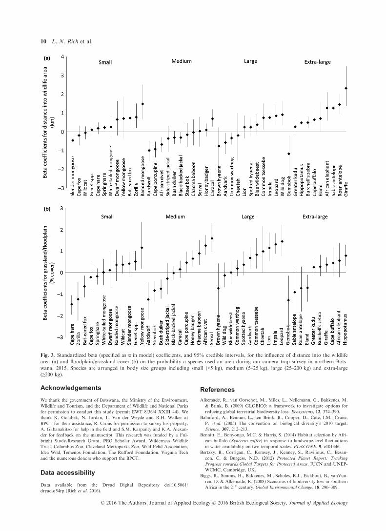
Of the 44 species photographed, 20 were strongly (i.e.

95% CI did not overlap zero) related to distance into the

wildlife area (14 positively and 6 negatively) and 23 to

percentage cover of floodplain/grassland (15 positively

and 8 negatively; Fig. 3). In contrast, occurrence of only

seven and one species were strongly related to the trap-

ping rate of humans/vehicles and distance to permanent

water, respectively (Appendix S1). As expected, precision

of estimates was lower for species with limited numbers of

detections, leading to diffuse posterior distributions for

their estimates of covariate effects.

Discussion

Our research highlights the importance of protected areas

and grasslands in maintaining biodiversity in southern

Africa (Millennium Ecosystem Assessment 2005; Biggs

et al. 2008; Craigie et al. 2010). We found overall species

richness was generally greater in floodplains and grass-

lands and areas located further into protected wildlife

areas (Table 1; Fig. 2). Our results support regional con-

servation initiatives focused on grasslands as this biome is

vulnerable to future land-use pressures (Biggs et al. 2008)

and benefits a broad diversity of species, including large-

bodied animals that are often threatened by hunting pres-

sure (Fa, Ryan & Bell 2005; Packer et al. 2009). Addition-

ally, over a quarter of the world’s grasslands have already

been lost (DeFries, Foley & Asner 2004) and the remain-

ing grasslands are threatened by woody encroachment

(Ratajzak, Nippert & Collins 2012). Our results also high-

light the importance of protected wildlife areas, particu-

larly to small- and large-bodied species, herbivores and

carnivores. While the effectiveness of protected areas is

mixed (Western, Russell & Cuthill 2009; Craigie et al.

2010; Kiffner, Stoner & Caro 2013), we found that live-

stock areas had lower levels of species richness and that

species richness increased with distance into protected

areas. These results are consistent with the trend of agri-

culture growth and habitat loss functioning as primary

threats to biodiversity world-wide (Millennium Ecosystem

Assessment 2005).

In northern Botswana, wildlife and livestock areas are

separated by the veterinary fence. The fence is permeable

to many species (e.g. carnivores) but impermeable or

semipermeable to others. When the fences were erected,

they cut-off migratory routes of wildebeests Connochaetes

taurinus and zebras Equus burchelli and disturbed the

movement patterns of additional ungulate species (Hay-

ward & Kerley 2009). If the fence, as a physical bound-

ary, was the underlying cause of increased species richness

in wildlife areas, then we would expect species richness to

be nearly constant between the core and edge of wildlife

areas (Kiffner, Stoner & Caro 2013). Our results showing

species richness increasing with distance from the fence,

however, (Fig. 2) suggest other spatial factors such as

land use and human–wildlife conflict (e.g. poaching and

retaliatory killings) are likely to be contributing drivers of

this edge effect (Woodroffe & Ginsberg 1998). Results

presented here suggest management of human activities

on both sides of protected area borders is essential for

minimizing edge effects (Woodroffe & Ginsberg 1998).

The weak effects of human/vehicle trap rates and water

accessibility on community-level species richness were sur-

prising (Table 1). The human/vehicle trap rate results

likely reflect that most of our study area was used by

tourists or tourism operators, all of whom seek out areas

with abundant wildlife. This human disturbance may have

had minimal impact on nocturnal species given that tour-

ism activities were generally restricted to daylight hours

(i.e. via Game Reserve permit rules). Distance to perma-

nent water had a weak effect on species richness in this

study, in contrast with other studies in Africa (Pettorelli

et al. 2010; Epps et al. 2011; Schuette et al. 2013). We

found wildlife to be more evenly distributed across the

landscape in relation to water availability perhaps because

(i) our study took place during the end of the wet season

and beginning of the dry season when water was less of a

limiting resource, (ii) we were unable to account for

ephemeral water sources and (iii) selection of high quanti-

ties of grass in wet areas vs. grass with higher nutrition in

dry areas is species dependent (Hopcraft et al. 2012).

In addition to community-level effects, our multi-spe-

cies approach allowed us to evaluate how specific groups

of species were influenced by human and environmental

factors. If managers wish to focus their efforts on con-

serving herbivores, for example, our research suggests

protected areas and heterogeneity in vegetation types

promote herbivore diversity. Similar to overall species

richness, we found herbivore richness increased with dis-

tance into wildlife areas (Table 2; Fig. 2). The influence

of grassland and floodplain cover, however, was highly

variable (Fig. 2). Species that are predominantly grazers,

such as zebras and impalas, were more likely to use

grasslands and floodplains where their food source was

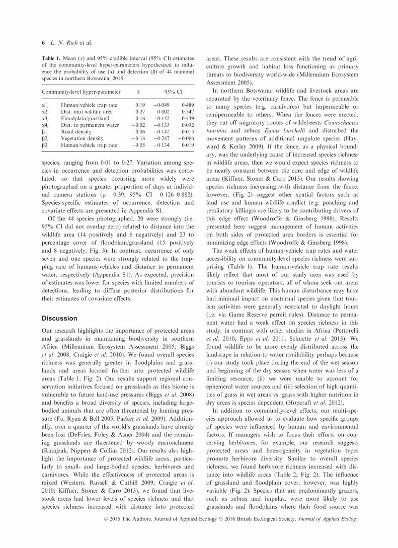
Table 1. Mean (�x) and 95% credible interval (95% CI) estimates

of the community-level hyper-parameters hypothesized to influ-

ence the probability of use (a) and detection (b) of 44 mammal

species in northern Botswana, 2015

Community-level hyper-parameter �x 95% CI

a1i Human/vehicle trap rate 0�19 �0�049 0�489a2i Dist. into wildlife area 0�27 �0�002 0�547a3i Floodplain/grassland 0�16 �0�142 0�439a4i Dist. to permanent water �0�02 �0�133 0�092b1i Road density �0�06 �0�142 0�015b2i Vegetation density �0�16 �0�247 �0�066b3i Human/vehicle trap rate �0�05 �0�134 0�019


6 L. N. Rich et al.

abundant. We found small ungulates including steenbok

Raphicerus campestris and bush duikers Sylvicapra grim-

mia, however, had a negative relationship with grasslands

and floodplains. These small grazers may select for mixed

shrub- and mopane-dominated areas because they are

adapted to selecting high-quality components of grass

Fig. 2. Mean, site-specific estimates of overall species richness and the richness of diet and body size (small < 5 kg, medium 5–25 kg,

large 25–200 kg and extra-large ≥ 200 kg) groups of species in relation to (a) the camera station’s distance into a protected wildlife area

(negative values indicate camera was in a livestock area) and (b) grassland/floodplain cover. Camera trap survey took place in Ngami-

land District, Botswana, 2015.



allowing them to forage in low biomass areas (Wilm-

shurst, Fryxell & Colucci 1999).

Our research can also be used to predict which groups

of species or individual species would be most impacted

by increasing levels of human disturbance in and outside

of protected areas. As hypothesized, we found extra-large

species like giraffes Giraffa camelopardalis and roan ante-

lopes Hippotragus equinus were most sensitive to human

disturbance where the probabilities of using an area

increased with distance into the wildlife area (Table 2,

Fig. 2). The groups of species that would likely be unaf-

fected or positively affected by increasing levels of human

disturbance were omnivores and medium-sized species

(Fig. 2), such as the African civet Civettictis civetta and

Fig. 2. Continued.


8 L. N. Rich et al.

jackal species (Fig. 3). Medium-sized omnivores tend to

be generalists that can use a wide array of landscapes and

thrive even after extensive human modification (Roemer,

Gompper & Van Valkenburgh 2009).

Reliable methods for evaluating biodiversity are key to

making informed conservation and management decisions

(Pettorelli et al. 2010; Zipkin et al. 2010). Equally impor-

tant is the need to understand how top-down (e.g.

humans) and bottom-up (e.g. vegetation cover) factors

influence diversity (Elmhagen & Rushton 2007). Our

research demonstrates the utility of camera trap surv-

eys and hierarchical models for assessing community,

group and individual species’ responses to both anthro-

pogenic and environmental variables. Our study did, how-

ever, have some potential limitations. First, our sequential

sampling of subareas may have violated the model’s

assumption of geographic closure (MacKenzie et al.

2002). A simulation study based on estimated occupancy

and detection probabilities from our pilot season, how-

ever, found this sampling design balanced precision of

occupancy estimates with survey effort. Secondly, because

we only included camera station-specific covariates, we

were unable to account for species-specific measures of

predation and competition, which are known to influence

species’ distributions (Caro & Stoner 2003). Lastly, we

sampled on sand roads to maximize detection probabili-

ties (Forman & Alexander 1998). If cameras had been

placed randomly, we believe the photographic rates of

many wildlife species, particularly carnivores, would have

been prohibitively low. However, if any species avoided

roads, then our sampling design may have resulted in

their true occupancy being underestimated.

Our multi-species approach provides a method for using

detection/non-detection data to estimate and evaluate spe-

cies’ occupancy and richness that should reduce money,

time and personnel costs, which are critical for many man-

agement agencies across the world where field data funding

is limited (Zipkin, DeWan & Royle 2009). Camera trap

surveys are an ideal field method for community studies on

terrestrial species because they photograph every species

that passes in front of them. Few studies, however, capital-

ize on this wealth of community information as attention

is typically focused on a single species or guild of species

(Stoner et al. 2007; Pettorelli et al. 2010; Schuette et al.

2013). Unlike traditional community analyses, our multi-

species approach allowed us to retain species identity while

properly accounting for multiple sources of uncertainty

(K�ery & Royle 2008; Zipkin et al. 2010). Many of the spe-

cies in our study had low detection probabilities which, if

left unaccounted for, would have resulted in underesti-

mates of species richness and affected estimates of our eco-

logical variables (Zipkin et al. 2010). Additionally, our

multi-species approach allowed us to integrate data across

species using the community-level hyper-parameter (Dora-

zio & Royle 2005; Russell et al. 2009; Zipkin, DeWan &

Royle 2009). This permitted us to complete a comprehen-

sive assessment of all wildlife species and resulted in

increased precision of species-specific occupancy probabili-

ties, particularly for species that were rarely photographed.

We suggest that broader application of this approach to

camera trap studies world-wide will likely result in a more

comprehensive and efficient use of available data and a

better understanding of the spatial ecology of all species

within the terrestrial wildlife community.

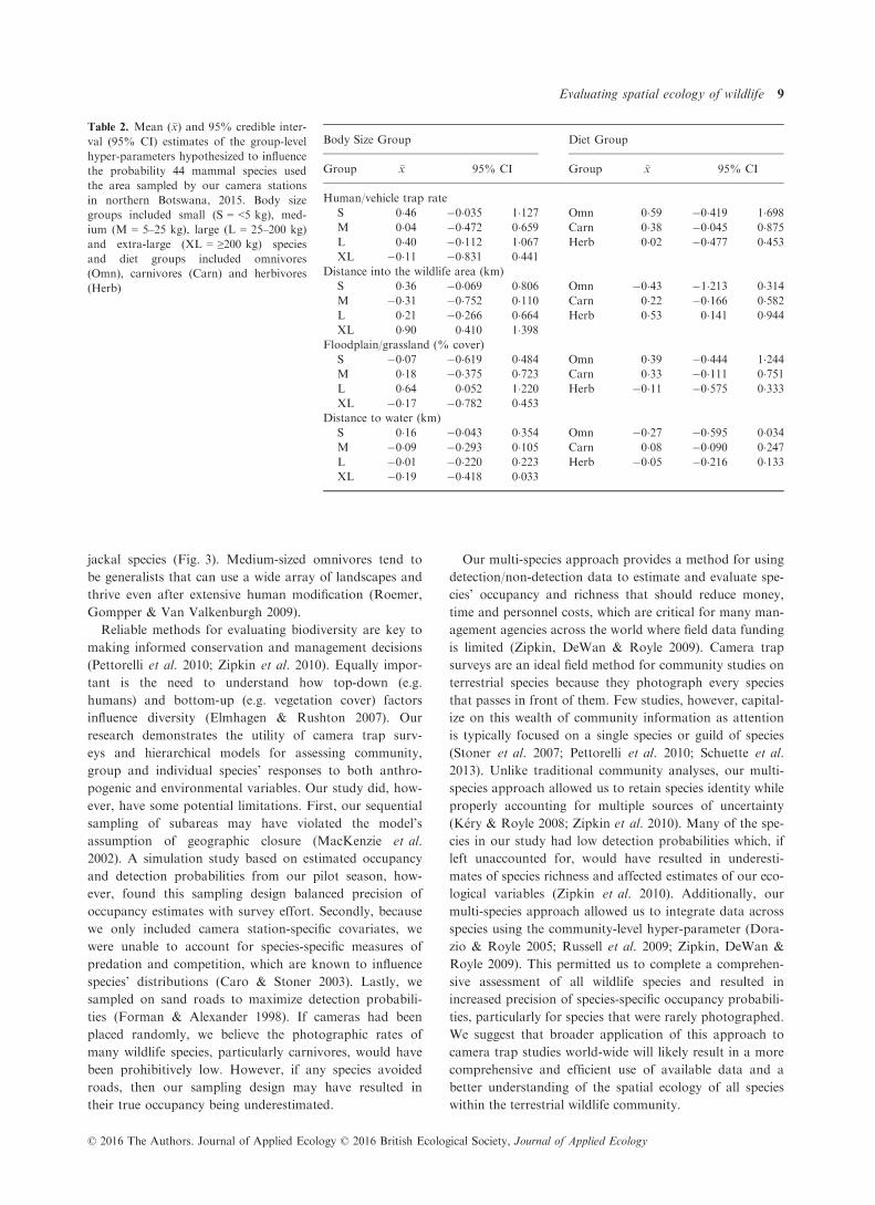
Table 2. Mean (�x) and 95% credible inter-

val (95% CI) estimates of the group-level

hyper-parameters hypothesized to influence

the probability 44 mammal species used

the area sampled by our camera stations

in northern Botswana, 2015. Body size

groups included small (S = <5 kg), med-

ium (M = 5–25 kg), large (L = 25–200 kg)

and extra-large (XL = ≥200 kg) species

and diet groups included omnivores

(Omn), carnivores (Carn) and herbivores

(Herb)

Body Size Group Diet Group

Group �x 95% CI Group �x 95% CI

Human/vehicle trap rate

S 0�46 �0�035 1�127 Omn 0�59 �0�419 1�698M 0�04 �0�472 0�659 Carn 0�38 �0�045 0�875L 0�40 �0�112 1�067 Herb 0�02 �0�477 0�453XL �0�11 �0�831 0�441

Distance into the wildlife area (km)

S 0�36 �0�069 0�806 Omn �0�43 �1�213 0�314M �0�31 �0�752 0�110 Carn 0�22 �0�166 0�582L 0�21 �0�266 0�664 Herb 0�53 0�141 0�944XL 0�90 0�410 1�398

Floodplain/grassland (% cover)

S �0�07 �0�619 0�484 Omn 0�39 �0�444 1�244M 0�18 �0�375 0�723 Carn 0�33 �0�111 0�751L 0�64 0�052 1�220 Herb �0�11 �0�575 0�333XL �0�17 �0�782 0�453

Distance to water (km)

S 0�16 �0�043 0�354 Omn �0�27 �0�595 0�034M �0�09 �0�293 0�105 Carn 0�08 �0�090 0�247L �0�01 �0�220 0�223 Herb �0�05 �0�216 0�133XL �0�19 �0�418 0�033



Acknowledgements

We thank the government of Botswana, the Ministry of the Environment,

Wildlife and Tourism, and the Department of Wildlife and National Parks

for permission to conduct this study (permit EWT 8/36/4 XXIII 44). We

thank K. Golabek, N. Jordan, L. Van der Weyde and R.H. Walker at

BPCT for their assistance, R. Crous for permission to survey his property,

A. Gabanakitso for help in the field and S.M. Karpanty and K.A. Alexan-

der for feedback on the manuscript. This research was funded by a Ful-

bright Study/Research Grant, PEO Scholar Award, Wilderness Wildlife

Trust, Columbus Zoo, Cleveland Metroparks Zoo, Wild Felid Association,

Idea Wild, Temenos Foundation, The Rufford Foundation, Virginia Tech

and the numerous donors who support the BPCT.

Data accessibility

Data available from the Dryad Digital Repository doi:10.5061/

dryad.q54rp (Rich et al. 2016).

References

Alkemade, R., van Oorschot, M., Miles, L., Nellemann, C., Bakkenes, M.

& Brink, B. (2009) GLOBIO3: a framework to investigate options for

reducing global terrestrial biodiversity loss. Ecosystems, 12, 374–390.Balmford, A., Bennun, L., ten Brink, B., Cooper, D., Cot�e, I.M., Crane,

P. et al. (2005) The convention on biological diversity’s 2010 target.

Science, 307, 212–213.Bennitt, E., Bonyongo, M.C. & Harris, S. (2014) Habitat selection by Afri-

can buffalo (Syncerus caffer) in response to landscape-level fluctuations

in water availability on two temporal scales. PLoS ONE, 9, e101346.

Bertzky, B., Corrigan, C., Kemsey, J., Kenney, S., Ravilious, C., Besan-

con, C. & Burgess, N.D. (2012) Protected Planet Report: Tracking

Progress towards Global Targets for Protected Areas. IUCN and UNEP-

WCMC, Cambridge, UK.

Biggs, R., Simons, H., Bakkenes, M., Scholes, R.J., Eickhout, B., vanVuu-

ren, D. & Alkemade, R. (2008) Scenarios of biodiversity loss in southern

Africa in the 21st century. Global Environmental Change, 18, 296–309.

Fig. 3. Standardized beta (specified as a in model) coefficients, and 95% credible intervals, for the influence of distance into the wildlife

area (a) and floodplain/grassland cover (b) on the probability a species used an area during our camera trap survey in northern Bots-

wana, 2015. Species are arranged in body size groups including small (<5 kg), medium (5–25 kg), large (25–200 kg) and extra-large

(≥200 kg).


10 L. N. Rich et al.

http://dx.doi.org/10.5061/dryad.q54rp

http://dx.doi.org/10.5061/dryad.q54rp

Caro, T.M. & Stoner, C.J. (2003) The potential for interspecific competi-

tion among African carnivores. Biological Conservation, 110, 67–75.Carroll, C., Noss, R.F. & Paquet, P.C. (2001) Carnivores as focal species

for conservation planning in the Rocky Mountain region. Ecological

Applications, 11, 961–980.Chandler, R.B., King, D.I., Raudales, R., Trubey, R., Chandler, C. &

Ch�avez, V.J.A. (2013) A small-scale land-sparing approach to conserv-

ing biological diversity in tropical agricultural landscapes. Conservation

Biology, 27, 785–795.Craigie, I.D., Baillie, J.E.M., Balmford, A., Carbone, C., Collen, B.,

Green, R.E. & Hutton, J.M. (2010) Large mammal declines in Africa’s

protected areas. Biological Conservation, 143, 2221–2228.Davies, K.F., Margules, C.R. & Lawrence, J.F. (2000) Which traits of spe-

cies predict population declines in experimental forest fragments? Ecol-

ogy, 81, 450–461.DeFries, R.S., Foley, J.A. & Asner, G.P. (2004) Land-use choices: balanc-

ing human needs and ecosystem function. Frontiers in Ecology and the

Environment, 2, 249–257.Dorazio, R.M. & Royle, J.A. (2005) Estimating size and composition of

biological communities by modeling the occurrence of species. Journal

of American Statistical Association, 100, 389–398.Elmhagen, B. & Rushton, S.P. (2007) Trophic control of mesopredators in

terrestrial ecosystems: top-down or bottom-up? Ecology Letters, 10,

197–206.Epps, C.W., Mutayoba, B.M., Gwin, L. & Brashares, J.S. (2011) An

empirical evaluation of the African elephant as a focal species for con-

nectivity planning in East Africa. Diversity and Distributions, 17, 603–612.

Estes, R.D. (1991) The Behavior Guide to African Mammals: Including

Hoofed Mammals, Carnivores, and Primates. The University of Califor-

nia Press, Berkeley.

Fa, J.E., Ryan, S.F. & Bell, D.J. (2005) Hunting vulnerability, ecological

characteristics and harvest rates of bushmeat species in afrotropical for-

ests. Biological Conservation, 121, 167–176.Forman, R.T.T. & Alexander, L.E. (1998) Roads and their major ecologi-

cal effects. Annual Review of Ecology and Systematics, 29, 207–231.Gard, T.C. 1984. Persistence in food webs. Mathematical Ecology (eds

S.A. Levin & T.G. Hallam), pp. 208–219. Springer Verlag, Berlin.Gaston, K.J. & Blackburn, T.M. (1996) Conservation implications of geo-

graphic range size-body size relationships. Conservation Biology, 10,

638–646.Gelman, A., Carlin, J.B., Stern, H.S. & Rubin, D.B. (2004) Bayesian Data

Analysis. Chapman and Hall, Boca Raton, FL.

Hayward, M.W. & Kerley, G.I.H. (2009) Fencing for conservation: restric-

tion of evolutionary potential or a riposte to threatening processes?

Biological Conservation, 142, 1–13.Hopcraft, J.G.C., Anderson, T.M., P�erez-Vila, S., Mayemba, E. & Olff,

H. (2012) Body size and the division of niche space: food and predation

differentially shape the distribution of Serengeti grazers. Journal of Ani-

mal Ecology, 81, 201–213.Kaunda, S.K.K. (2001) Spatial utilization by black-backed jackals in

southeastern Botswana. African Zoology, 36, 143–152.Keene-Young, R. (1999) A thin line: Botswana’s cattle fences. Africa Envi-

ronment and Wildlife, 7, 71–79.K�ery, M. & Royle, J.A. (2008) Hierarchical Bayes estimation of species

richness and occupancy in spatially replicated surveys. Journal of

Applied Ecology, 45, 589–598.Kiffner, C., Stoner, C. & Caro, T. (2013) Edge effects and large mammal

distributions in a national park. Animal Conservation, 16, 97–107.Lambeck, R.J. (1997) Focal species: a multi-species umbrella for nature

conservation. Conservation Biology, 11, 849–856.MacKenzie, D.I., Nichols, J.D., Lachman, G.B., Droege, S., Royle, J.A. &

Langtimm, C.A. (2002) Estimating site occupancy rates when detection

probabilities are less than one. Ecology, 83, 2248–2255.Mbaiwa, J.E., Stronza, A. & Kreuter, U. (2011) From collaboration to

conservation: insights from the Okavango Delta, Botswana. Society and

Natural Resources, 24, 400–411.Millennium Ecosystem Assessment (2005) Ecosystems and Human Well-

Being: Biodiversity Synthesis. World Resources Institute, Washington,

DC.

Packer, C., Kosmala, M., Cooley, H.S., Brink, H., Pintea, L., Garshelis,

D. et al. (2009) Sport hunting, predator control and conservation of

large carnivores. PLoS ONE, 4, e5941.

Pettorelli, N., Lobora, A.L., Msuha, M.J., Foley, C. & Durant, S.M.

(2010) Carnivore biodiversity in Tanzania: revealing the distribution

patterns of secretive mammals using camera traps. Animal Conservation,

13, 131–139.Plummer, M. (2011) JAGS: a program for the statistical analysis of Baye-

sian hierarchical models by Markov Chain Monte Carlo. Available

from http://sourceforge.net/projects/mcmc-jags/ (accessed August 2015).

Ratajzak, Z., Nippert, J.B. & Collins, S.L. (2012) Woody encroachment

decreases diversity across North American grasslands and savannas.

Ecology, 93, 697–703.Rich, L.N., Miller, D.A.W., Robinson, H.S., McNutt, J.W. & Kelly, M.K.

(2016) Data from: using camera trapping and hierarchical occupancy mod-

elling to evaluate the spatial ecology of an African mammal community.

Dryad Digital Repository, http://dx.doi.org/10.5061/dryad.q54rp.

Ripple, W.J., Estes, J.A., Beschta, R.L., Wilmers, C.C., Ritchie, E.G.,

Hebblewhite, M. et al. (2014) Status and ecological effects of the

world’s largest carnivores. Science, 343, 151–162.Roemer, G.W., Gompper, M.E. & Van Valkenburgh, B. (2009) The eco-

logical role of the mammalian mesocarnivore. BioScience, 59, 165–173.Royle, J.A. & Nichols, J.D. (2003) Estimating abundance from repeated

presence-absence data or point counts. Ecology, 84, 777–790.Russell, R.E., Royle, J.A., Saab, V.A., Lehmkuhl, J.F., Block, W.M. &

Sauer, J.R. (2009) Modeling the effects of environmental disturbance on

wildlife communities: avian responses to prescribed fire. Ecological

Applications, 19, 1253–1263.Schuette, P., Wagner, A.P., Wagner, M.E. & Creel, S. (2013) Occupancy

patterns and niche partitioning within a diverse carnivore community

exposed to anthropogenic pressures. Biological Conservation, 158, 301–312.

Simberloff, D. (1998) Flagships, umbrellas, and keystones: is single-species

management passe in the landscape era? Biological Conservation, 83,

247–257.Stoner, C., Caro, T., Mduma, S., Mlingwa, C., Sabuni, G. & Borner, M.

(2007) Assessment of effectiveness of protection strategies in Tanzania

based on a decade of survey data for large herbivores. Conservation

Biology, 21, 635–646.Western, D., Russell, S. & Cuthill, I. (2009) The status of wildlife in protected

areas compared to non-protected areas of Kenya. PLoS ONE, 4, e6140.

Wiens, J.A., Hayward, G.D., Holthausen, R.S. & Wisdom, M.J. (2008)

Using surrogate species and groups for conservation planning and man-

agement. BioScience, 58, 241–252.Wilmshurst, J.F., Fryxell, J.M. & Colucci, P.E. (1999) What constrains

daily intake in Thomson’s gazelles? Ecology, 80, 2338–2347.Woodroffe, R. & Ginsberg, J.R. (1998) Edge effects and the extinction of

populations inside protected areas. Science, 280, 2126–2128.Yoccoz, N.G., Nichols, J.D. & Boulinier, T. (2001) Monitoring of biologi-

cal diversity in space and time. Trends in Ecology and Evolution, 16,

446–453.Zipkin, E.F., DeWan, A. & Royle, J.A. (2009) Impacts of forest fragmen-

tation on species richness: a hierarchical approach to community model-

ing. Journal of Applied Ecology, 46, 815–822.Zipkin, E.F., Royle, J.A., Dawson, D.K. & Bates, S. (2010) Multi-species

occurrence models to evaluate the effects of conservation and manage-

ment actions. Biological Conservation, 143, 479–484.

Received 22 November 2015; accepted 11 March 2016

Handling Editor: Matt Hayward

Supporting Information

Additional Supporting Information may be found in the online version

of this article.

Appendix S1. Species-specific probabilities of occurrence, proba-

bilities of detection and the effects of anthropogenic and habitat

covariates.

Appendix S2. Hierarchical group model JAGS code.

Appendix S3. Camera station-specific estimates of species rich-

ness, including overall community, carnivore, omnivore, herbi-

vore, small (<5 kg), medium (5–25 kg), large (25–200 kg), and

extra-large (>200 kg) species richness.



http://sourceforge.net/projects/mcmc-jags/

http://dx.doi.org/10.5061/dryad.q54rp.

journal of applied ecology using camera trapping and ... camera trapping and...camera trap studies...

Documents