Satellite galaxies around present-day massive ellipticals

Journal: Monthly Notices of the Royal Astronomical Society

Manuscript ID: MN-13-3244-MJ.R2

Manuscript type: Main Journal

Date Submitted by the Author: n/a

Complete List of Authors: Ruiz, Pablo; Universidad de La Laguna, Departamento de Astrofísica Trujillo, Ignacio; Instituto de Astrofísica de Canarias, Mármol-Queraltó, Esther; Instituto de Astrofísica de Canarias, ; Universidad de La Laguna, Departamento de Astrofísica; University of Edinburgh, Institute for Astronomy

Keywords: galaxies: formation < Galaxies, galaxies: elliptical and lenticular, cD < Galaxies, galaxies: evolution < Galaxies, galaxies: luminosity function, mass function < Galaxies

Mon. Not. R. Astron. Soc. 000, 1–?? (2013) Printed 24 April 2014 (MN LATEX style file v2.2)

Satellite galaxies around present-day massive ellipticals

Pablo Ruiz1 ⋆, Ignacio Trujillo1,2 and Esther Marmol-Queralto1,2,3

1Departamento de Astrofısica, Universidad de La Laguna, E-38205, La Laguna, Tenerife, Spain2Instituto de Astrofısica de Canarias, c/ Vıa Lactea s/n, E-38205, La Laguna, Tenerife, Spain3 Institute for Astronomy, University of Edinburgh, Royal Observatory, Edinburgh, EH9 3HJ

ABSTRACT

Using the spectroscopic NYU-VAGC and the photometric PHOTOZ catalogues of theSloan Digital Sky Survey (SDSS DR7), we have explored the satellite distribution around∼1000 massive (M⋆&2×1011M⊙) visually classified elliptical galaxies down to a satellite massratio of 1:400 (i.e. 5×108

.Msat.2×1011M⊙). Our host galaxies were selected to be represen-tative of a mass complete sample. The satellites of these galaxies were searched within aprojected radial distance of 100 kpc to their hosts. We have found that only 20-23% of themassive ellipticals has at least a satellite down to a mass ratio 1:10. This number increasesto 45-52% if we explore satellites down to 1:100 and is >60-70% if we go further downto 1:400. The average projected radial distance of the satellites to their hosts for our wholesample down to 1:400 is ∼59 kpc (which can be decreased at least down to 50 kpc if we ac-count for incompleteness effects). The number of satellites per galaxy host only increases verymildly at decreasing the satellite mass. The fraction of mass which is contained in the satel-lites down to a mass ratio of 1:400 is 8% of the total mass contained by the hosts. Satelliteswith a mass ratio from 1:2 to 1:5 (with ∼28% of the total mass of the satellites) are the maincontributor to the total satellite mass. If the satellites eventually infall into the host galaxies,the merger channel will be largely dominated by satellites with a mass ratio down to 1:10 (asthese objects have 68% of the total mass in satellites).

Key words: galaxies: evolution – galaxies: formation – galaxies: elliptical and lenticular, cD– galaxies: luminosity function, mass function

1 INTRODUCTION

A combination of major and minor merging has raised in the last

few years as the most likely channel of size and mass growth of

present-day massive (M⋆&1011M⊙) ellipticals. A number of obser-

vational as well as theoretical studies support this mode of growth.

According to that picture, present-day most massive ellipticals cre-

ated the bulk of their mass in a short but very intense starburst event

at z&2 (e.g. Keres et al. 2005; Dekel et al. 2009; Oser et al. 2010;

Ricciardelli et al. 2010; Wuyts et al. 2010; Bournaud et al. 2011).

The initial structural configuration of these galaxies was very com-

pact. Later on, a continuous bombardment process by the satellites

orbiting these objects produced the envelopes that we see today sur-

rounding these galaxies (Khochfar & Silk 2006; Oser et al. 2010;

Feldmann et al. 2011). There are several observations that fits well

within this scheme. To name a few, we have for example evidences

for a progressive size evolution of the massive galaxies since z∼3

(e.g. Trujillo et al. 2007; Buitrago et al. 2008) produced mainly by

the formation of the outer regions (e.g. Bezanson et al. 2009; Hop-

kins et al. 2009a; van Dokkum et al. 2010). We also have evidences

⋆ E-mail: ruihern@gmail

showing that the size evolution of the massive galaxies does not

depend on the age of their stellar populations (Trujillo et al. 2011)

nor in their intrinsic sizes (Dıaz-Garcıa et al. 2013), suggesting a

growth mechanism external to the galaxy properties. Moreover, the

average velocity dispersion of the massive galaxy population has

decreased mildly since z∼2, in good agreement with the theoreti-

cal expectations based on galaxy merging (e.g. Cenarro & Trujillo

2009). All these results have made more unlikely that the chan-

nel growth of massive galaxies could be driven by AGN or super-

nova feedback (Fan et al. 2008, 2010; Ragone-Figueroa & Granato

2011). Nonetheless, all the above observational evidences test the

growth of massive galaxies only indirectly. It is timely then to con-

duct a detailed analysis of the properties of the satellites that pro-

mote the growth of the massive galaxy population.

Several works have studied in detail what are the properties of

the satellites surrounding the massive elliptical galaxies over cos-

mic time (Jackson et al. 2010; Nierenberg et al. 2011; Nierenberg

et al. 2013; Man et al. 2012; Newman et al. 2012; Marmol-Queralto

et al. 2012, 2013; Huertas-Company et al. 2013). Marmol-Queralto

et al. (2012) have found that the fraction of massive galaxies with

satellites of a given mass ratio (1:100 up to z=1 and 1:10 up to

z=2) has remained constant with time. This constancy of the num-

ber of satellites surrounding the massive galaxies is in good agree-

c© 2013 RAS

Page 1 of 15

123456789101112131415161718192021222324252627282930313233343536373839404142434445464748495051525354555657585960

2 Pablo Ruiz, Ignacio Trujillo & Esther Marmol-Queralto

ment with semianalytical predictions based on the ΛCDM scenario

(Quilis & Trujillo 2012). However, the theoretical estimates over-

predict the fraction of massive galaxies with satellites down to

1:100 mass ratio by a factor of ∼2. It is unclear though how rel-

evant could be the effects of incompleteness in the observational

studies.

The goal of this paper is to create a local (z∼0) reference

that can be used to anchor the evolution of the satellite population

of massive galaxies at higher redshifts. In particular, we concen-

trate on this paper on present-day massive ellipticals which are the

galaxies which show the largest size evolution with cosmic time.

To facilitate the comparison with high-z studies, the way this local

reference of massive elliptical galaxies is created is based only on

the visual morphology of the galaxies. We do not make any color

selection of our galaxies to avoid biasing our sample towards either

young or old galaxies. In addition, we do not make any previous

selection of our sample based on environmental density criteria. To

reach our aim, we have used the morphological galaxy catalogue of

Nair & Abraham (2010). Due to the vicinity of our objects (z<0.1),

we can probe the satellite distribution of these massive ellipticals

down to a satellite stellar mass Msat∼5×108M⊙. Our work also

includes another necessary exercise. We have explored the differ-

ences between the satellite populations when using a purely spec-

troscopic redshift sample or a photometric redshift one. This com-

parison is worth doing as in higher redshift samples the ability of

selecting satellites using spectroscopic data alone is severely com-

promised by the faint apparent magnitudes of these objects.

Although it is not our primary goal, the large number of mas-

sive galaxies studied in this paper could be used in future works to

make a direct test of the ΛCDM predictions about the number of

satellites surrounding the most massive galaxies in the present-day

Universe (see for instance Liu et al. 2011; Wang & White 2012).

Finally, our study will allow us to explore which is the most likely

merging channel of present-day massive ellipticals. We will quan-

tify which type of satellites will contribute most to the mass in-

crease of their host galaxies in case they eventually merge with

the main object. Undoubtedly, this local study, together with other

works at higher z (see e.g. Ferreras et al. 2013), will allow us to

explore whether the merging channel (i.e. which type of satellite

is the most likely to contribute to the mass and size growth) has

changed with time or not.

The paper is structured as follows. In Section 2, we describe

our sample of massive and satellite galaxies. Section 3 explains

the satellite selection criteria and the methods used to clean our

sample from background and clustering effects. Our main results

are presented in Sect. 4. The distribution of the mass contained in

satellites surrounding the massive ellipticals is shown in Section 5.

Section 6 discusses the main results of this paper and finally our

work is summarized in Sect.7. Hereafter, we assume a cosmology

with Ωm = 0.3, ΩΛ = 0.7 and H0 = 70 km s−1 Mpc−1.

2 THE DATA

Our study is based on two different datasets: the sets of massive

elliptical (host) galaxies and the samples of satellites around them.

On what follows, we describe how these samples were obtained.

2.1 Samples of massive elliptical galaxies

Our samples of massive elliptical galaxies have been obtained from

the morphological catalogue published by Nair & Abraham (2010)

(hereafter NA10). This catalogue comprises 14034 galaxies with

detailed visual classification and available spectra from the Sloan

Digital Sky Survey (SDSS) DR4 (Adelman-McCarthy et al. 2006)

in the spectroscopic redshift range 0.01<z<0.1 down to an apparent

extinction-corrected limit of g<16 mag. Within this catalogue, we

select the elliptical galaxies (i.e. c0, E0 and E+; T-Type class −5),

obtaining a sample of 2723 visually classified elliptical galaxies.

In order to have the more up to date spectroscopic redshift deter-

mination for these galaxies, we cross correlated that catalogue with

the spectroscopic NYU Value-Added Galaxy Catalogue (Blanton et

al. 2005) (NYU VAGC) based on the SDSS DR7 (Abazajian et al.

2009), obtaining 2654 galaxies common in both data sets.

In addition to a visual classification of the galaxies, the cata-

logue from NA10 provides other important parameters as their stel-

lar mass (based on Kauffmann et al. 2003). For consistency with the

catalogue of satellite galaxies where we have estimated the stellar

masses using the Bell et al. (2003) recipe, we have also measured

the stellar mass of our host elliptical galaxies using the same tech-

nique. This is done as follows. We take the SDSS bands magni-

tudes of our objects corrected from Galactic extinction (Schlegel

et al. 1998). Later on, we apply the K-correction provided by the

NYU VAGC (Blanton & Roweis 2007) both in the r-band and

in the g-r color in order to have these two magnitudes measured

in the rest-frame of our objects. Then, using the prescription of

Bell et al. (2003) we estimate the M/L ratio as a function of the

restframe color, assuming a Kroupa (2001) initial mass function

(IMF)1. Thus, the mass-to-luminosity ratio in the r−band is esti-

mated like this:

log(M/L)r = ar − br(g − r) − 0.15 (1)

where ar = −0.306 and br = 1.097 are the specific coefficients

applied to SDSS for determining the M/L ratio in the r-band and

0.15 is subtracted to get the results assuming a Kroupa IMF.

After computing (M/L)r, we can directly estimate the stellar

mass using the next relation:

log(M/M⊙) = log(M/L)r − 0.4(Mr − M⊙ ,r) (2)

where Mr is the absolute magnitude of the galaxy and

M⊙ ,r=4.68 the absolute magnitude of the Sun in the SDSS r−band.

We have compared our stellar mass estimates with the measure-

ments provided by NA10. We obtain the following results: our stel-

lar masses derived with Bell et al. (2003) are above (0.09 dex) than

those derived by NA10 which are based on Kauffmann et al. (2003).

This is not surprising taking into account the different methodolo-

gies and stellar population models used in both estimates of the

stellar mass. The mean difference between both stellar mass deter-

mination has a scatter of 0.1 dex. We consider this value as our

typical uncertainty at estimating the stellar mass of our host galax-

ies.

Once we have the stellar masses as well as the spectroscopic

redshifts of our host galaxies, we build a mass complete subsample

of host galaxies within a given redshift range. There is some obser-

vational evidence suggesting that the satellite population could de-

pend on the mass of their host galaxies (e.g. Wang & White 2012).

Consequently, if our host sample were not complete in mass, we

will be mixing hosts with different satellite populations along our

redshift range of exploration, eventually biasing our results. The

1 We have selected this IMF to facilitate the comparison of our results with

previous results conducted at higher redshift (e.g. Marmol-Queralto et al.

2012) and with numerical simulations (e.g. Quilis & Trujillo 2012).

c© 2013 RAS, MNRAS 000, 1–??

Page 2 of 15

123456789101112131415161718192021222324252627282930313233343536373839404142434445464748495051525354555657585960

Satellite galaxies around present-day massive ellipticals 3

building of this complete subsample of host galaxies is done as fol-

lows. In the stellar mass - redshift plane (see Fig. 1; upper panel),

we select which combination of stellar mass and redshift maxi-

mizes the number of massive galaxies within those ranges. We find

1017 massive ellipticals above 1.1×1011 M⊙ and z<0.064. This is

the sample of host galaxies that we will use in the rest of the paper

when referring to the spectroscopic host sample.

We have repeated the above exercise but this time using pho-

tometric redshifts for the host galaxies. We have conducted this

exercise since we are pushing the analysis of the satellite popula-

tion down to faint magnitudes where the redshift determination is

only photometric. For this reason, for consistency, is necessary to

have also the redshifts and the stellar masses of the host galaxies

determined using photometric redshifts as well. It is worth noting

that the sample of host galaxies built that way is related with the

spectroscopic sample but it does not necessary contain the same

all galaxies. For instance, the source of photometric redshifts we

have used (which we will describe later) provides larger redshifts

(z&0.04) for the host galaxies than the ones measured spectroscop-

ically. As the photometric redshifts estimation has its own biases

and uncertainties, our analysis using the photometric sample is

fully independent of the spectroscopic analysis. In fact, this analy-

sis has to be considered as an alternative analysis to the one using

the spectroscopic sample. In other words, the exercise conducted in

this paper explores how different the results would be in case we

were only having spectroscopic or photometric redshifts. Nonethe-

less, throughout the paper we will often compare both analysis to

check the consistency of our results. The building of the mass com-

plete subsample in the case of the photometric sample is done as

in the spectroscopic case. In the photometric stellar mass - redshift

plane (see Fig. 1; bottom panel), the sample is maximized (1147

objects) for masses above 1.9×1011 M⊙ and z<0.078. The spectro-

scopic and photometric sample have 696 hosts in common (i.e.

∼65% of the sample).

2.2 Samples of satellite galaxies

The samples of satellites surrounding our host galaxies are based

on the following two criteria: their stellar mass and their proximity

(both in spatial projected distance as well as in redshift) to our host

galaxies. We will describe in Section 3 what are the exact criteria

in distance and redshift used to select our satellite candidates. In

this section, we describe how the redshift and stellar mass have

been determined for the pull of galaxies that are used to select the

satellite candidates.

As the basis for the redshifts of our potential satellite galax-

ies we have used both the spectroscopic NYU VAGC and pho-

tometric (’PHOTOZ’) redshift catalogues of the SDSS DR7. The

NYU VAGC based on the SDSS DR7 spectroscopic database con-

tains over 900000 spectroscopically confirmed galaxies and it is

roughly complete down to r∼17.7 mag. Similarly, our photomet-

ric catalogue comprises the galactic ’primary’ sources with photo-

metrically estimated redshifts and K-corrections from ’PHOTOZ’

database. This is a large and continuous dataset of galaxies within

the SDSS DR7 coverage and whose 95% completeness2 is esti-

mated to be around r∼21.5 mag. The photometric redshift uncer-

tainty is 0.022.

As mentioned before, we have estimated the stellar masses

of our satellite candidates using the prescription given by Bell

2 http://www.sdss.org/dr7/products/general/completeness.html

0.0 0.2 0.4 0.6 0.8 1.0 1.2 1.4Lookback Time (Gyr)

10.5

11.0

11.5

12.0

log(

M/M

O •)

Spectroscopic Sample

N= 1017z < 0.064

log(M/MO •) > 11.045

0.02 0.04 0.06 0.08 0.10z

10.0

10.5

11.0

11.5

12.0

log(

M/M

O •)

Photometric Sample

0.02 0.04 0.06 0.08 0.10z

10.0

10.5

11.0

11.5

12.0

log(

M/M

O •)

N= 1147z < 0.078

log(M/MO •) > 11.278

Figure 1. Stellar mass vs. redshift for the massive elliptical (host) galaxies

of our spectroscopic (upper panel) and photometric (lower panel) samples.

The vertical and horizontal red dashed lines establish the maximum redshift

and minimum mass limits used in this paper to maximize the number of

massive elliptical galaxies within a complete mass subsample.

et al. (2003). This prescription is based on the g-r color. Conse-

quently, we need to account for the photometric errors both in

the g and r bands in order to assure this color is measured with

enough confidence to provide reliable stellar mass estimates. For

this reason, in addition to the magnitude limit in the r-band we

have used above, we also demand that the photometric errors at

estimating the number counts of each galaxy will be less than

3σ the expected error at measuring their number counts. In other

words, acceptable photometric errors for each object are those

where error(counts).3×sqrt(counts+σsky2). σsky is the uncertainty

(in counts) at measuring the sky value in each band3. Those galax-

ies in our catalogue which show photometric errors larger than

those values (in any of the two bands) are discarded from the anal-

ysis as their large errors could be linked to artifacts in the image:

proximity to bright nearby companions, etc. The number of galax-

3 Typical values for the sky in the SDSS images are: 24.88 counts (g-band)

and 23.96 counts (r-band). We have used the following set of equations to

transform our magnitudes and error(mag) provided by the catalogues into

counts and error(counts):

mag = −2.5 log

(

counts

exptime100.4(aa+kk×airmass)

)

(3)

error(mag) =2.5

ln 10

error(counts)

counts(4)

with exptime=53.907456 seconds and aa (zeropoint), kk (extinction coeffi-

cient) and airmass provided for each object.

c© 2013 RAS, MNRAS 000, 1–??

Page 3 of 15

123456789101112131415161718192021222324252627282930313233343536373839404142434445464748495051525354555657585960

4 Pablo Ruiz, Ignacio Trujillo & Esther Marmol-Queralto

0.02 0.03 0.04 0.05 0.06 0.07z

8

9

10

11

12

log(

M/M

O •)

0.02 0.03 0.04 0.05 0.06 0.07z

8

9

10

11

12

log(

M/M

O •)

log(M/MO •) ~ 11.05log(M/MO •) ~ 10.23log(M/MO •) ~ 10.17

0 2 4 6 8n (x 102)

0.060<z<0.064

2 4 6 8n (x 102)

Figure 2. Left panel: Stellar mass distribution vs. redshift for the galaxies in

the NYU VAGC spectroscopic catalogue. We plot in grey the galaxies found

within the spectroscopic catalogue. The pink points correspond to our sam-

ple of host massive elliptical galaxies. Right panel: Stellar mass distribution

for the spectroscopic catalogue in the redshift interval 0.060 < z < 0.064

(plotted in black in the left panel). This redshift range corresponds to the

limiting redshift we have used for the host galaxies in our spectroscopic

sample (see Fig. 1). The red dashed line is the estimated completeness limit

∼1.5×1010M⊙ whereas the blue line represents the minimum stellar mass

estimated for the sample of massive elliptical galaxies (∼1.1×1011M⊙). A

conservative estimate for the stellar mass completeness of the spectroscopic

sample is provided by the green dashed line: ∼1.7×1010M⊙ (see text for de-

tails).

ies rejected due to large photometric errors are: 4.1% in g-band and

4.5% in r-band.

Finally, there is a number of satellites candidates which are

bright enough (r<17.7 mag) to have a spectroscopic redshift deter-

mination. Consequently, we can divide our analysis of the satellite

galaxies in two subsamples: one where the redshift of the satellites

have been determined spectroscopically and one where we have

used the photometric redshift determination. In the following sub-

sections we explore what are the characteristics of each subsample.

2.2.1 Stellar mass completeness for the spectroscopic catalogue

Once the stellar masses of the galaxies of the sample are deter-

mined we can estimate down to which stellar mass our catalogue

of galaxies is complete. In this subsection we do such analysis for

the spectroscopic catalogue. We conduct the same exercise for the

photometric sample in the following subsection.

In the left panel of Fig. 2, we present the stellar mass versus

the spectroscopic redshift for the galaxies in the NYU VAGC. In

order to estimate the mass completeness of this sample, we have

explored the mass distribution of the galaxies at the upper limit of

our host galaxies redshift range (i.e. 0.06<z<0.064). This is shown

in the right panel of Fig. 2. The mass completeness limit is given

by the position of the peak of the mass distribution. We estimate

that peak evaluating the mode of the distribution. The stellar mass

completeness limit for our spectroscopic catalogue is placed on

log(M⋆/M⊙)∼10.17 at z=0.064. Above this mass value, we can

study the satellite population with completeness up to z=0.064.

This value of mass corresponds roughly to a mass ratio of 1:10

(0.1 < MSat /MHost < 1) for the satellite population.

2.2.2 Stellar mass completeness for the photometric catalogue

We now conduct the same completeness analysis but this time us-

ing the PHOTOZ SDSS DR7 photometric catalogue. In the left

panel of Fig. 3, we present the distribution of the stellar mass re-

spect to redshift of the galaxies in the photometric catalogue. As

we did with the spectroscopic catalogue, we explore the distribu-

tion of the stellar masses of our galaxies up to the upper limit of

our redshift distribution (in this case z=0.078). The right panel

of Fig. 3 shows the stellar mass distribution within the redshift

interval 0.074<z<0.078. The stellar mass completeness limit (es-

timated as the mode of the distribution in that redshift interval)

is established in log(M⋆/M⊙)∼8.78. This value indicates that we

can explore with completeness the distribution of satellites around

our host massive ellipticals down to a mass ratio of ∼1:330 (i.e.

0.003 < MSat/MHost < 1.0).

It is worth noting, however, that both in the spectroscopic and

the photometric catalogues, there is a potential bias to miss the old-

est galaxies at a fixed stellar mass. This is because both catalogues

are complete in redshift down to a given apparent r-band magni-

tude. In the case of the spectroscopic catalogue this is r∼17.7 (90%

completeness) and in the case of the photometric sample is r∼21.5

(95% completeness). These numbers translate into the following

K-corrected absolute magnitude values for each of the samples at

z=0.064: Mr=-19.7 mag in the case of the spectroscopic sample

and Mr=-16.4 mag at z=0.078 for the photometric catalogue. To

transform these absolute magnitude values into stellar mass limit

we need to have an estimation of the stellar mass-to-light ratio of

our galaxies. We have estimated which is the average g-r color for

our host galaxies and for our potential satellites. We find that our

host (∼1011M⊙) galaxies have a typical (g-r)∼0.85 whereas our less

massive (∼109M⊙) galaxies are bluer (g-r)∼0.70. Let’s assume now

a very conservative age for the less massive galaxies of 12 Gyr.

Using the MIUSCAT SEDs developed by Vazdekis et al. (2012)

and Ricciardelli et al. (2012), with the above color and age and

a Kroupa IMF, the largest (M/L)r ratio for these objects will be

around 3. This translates into the following stellar mass figures for

our stellar mass completeness: log(M⋆/M⊙)∼10.23 for the spectro-

scopic catalogue (i.e. a mass ratio of 1:7) and log(M⋆/M⊙)∼8.89 for

the photometric catalogue (i.e. a mass ratio of 1:250). On what fol-

lows, we will consider these values as the most conservative mass

completeness limits of our satellite galaxies.

3 SATELLITE SELECTION CRITERIA

Both for the spectroscopic and photometric catalogues we have ap-

plied the following procedure for identifying the satellite galaxies

around our host objects:

• We detect all the galaxies in the SDSS catalogues which are

within a projected radial distance to our central galaxies of R=100

kpc. This corresponds to a radius of 4.1 and 1.13 arcmin at z=0.02

and z=0.078, respectively. To avoid any bias due to the borders of

the SDSS survey, we only have considered host galaxies such as

the area enclosed by the satellite’s search radius is fully contained

within the catalogue borders. Our adopted search radius of 100 kpc

is a compromise between having a large area for finding a signif-

icant number of satellite candidates gravitationally bound to our

central massive galaxies but not as large as to be severely contami-

nated by background and foreground objects (see Sec. 3.1).

• The absolute difference between the satellite redshifts and the

redshift of the central galaxies must be lower than 0.0033 (in the

c© 2013 RAS, MNRAS 000, 1–??

Page 4 of 15

123456789101112131415161718192021222324252627282930313233343536373839404142434445464748495051525354555657585960

Satellite galaxies around present-day massive ellipticals 5

0 2 4 6 80 2 4 6 8n (x 104)

0.074<z<0.078

0.02 0.03 0.04 0.05 0.06 0.07z

8

9

10

11

12

log(

M/M

O •)

log(M/MO •) ~ 8.78log(M/MO •) ~ 8.89log(M/MO •)~ 11.28

log(M/MO •) ~ 8.78log(M/MO •) ~ 8.89log(M/MO •)~ 11.28

0.02 0.03 0.04 0.05 0.06 0.07z

8

9

10

11

12

log(

M/M

O •)

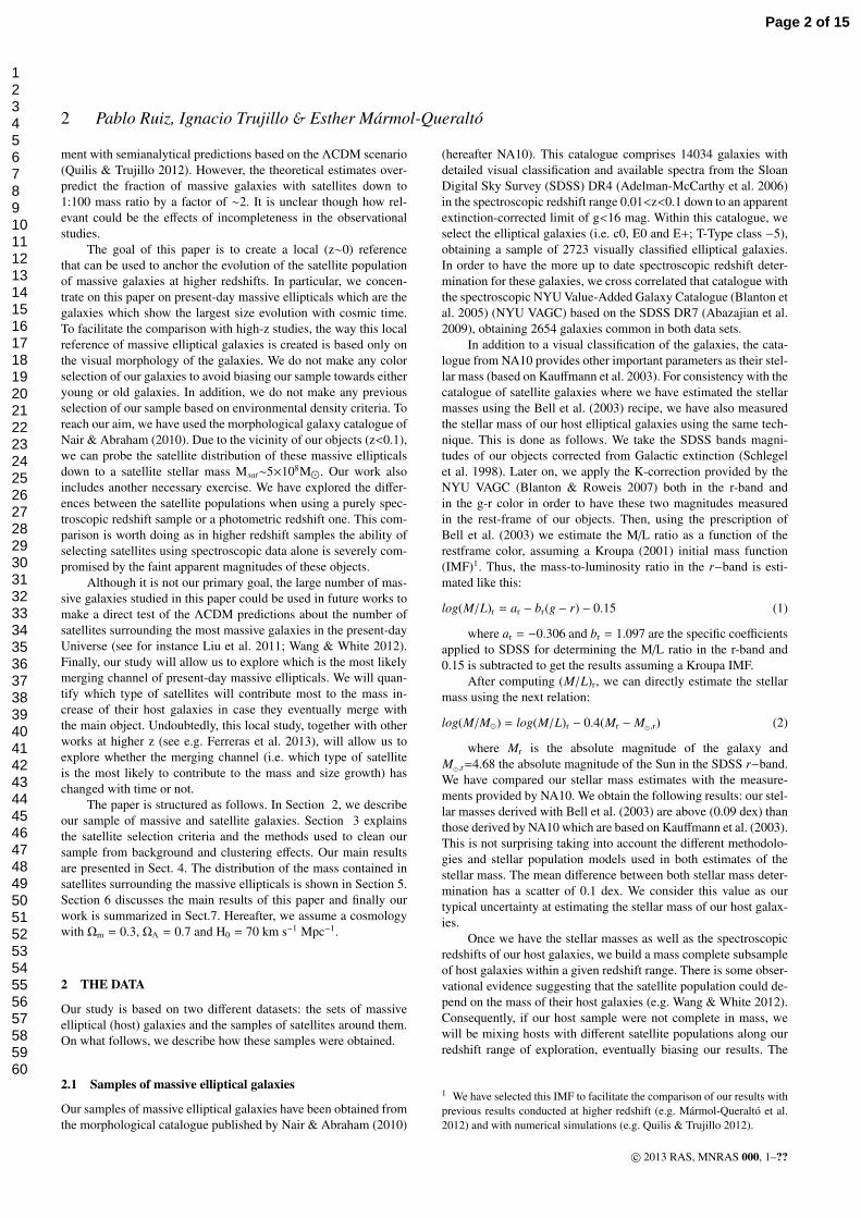
Figure 3. Left panel: Stellar mass distribution vs. redshift for the galaxies in

the photometric PHOTOZ SDSS DR7 catalogue. The galaxies of the pho-

tometric sample are represented in grey. The pink distribution corresponds

to our sample of host massive elliptical galaxies. Right panel: Histogram of

the stellar mass distribution of galaxies in the photometric catalogue in the

redshift interval 0.074 < z < 0.078 (plotted in black in the left panel). This

redshift range corresponds to the limiting redshift we have used for the host

galaxies in our photometric sample (see Fig. 1). The red dashed line is the

estimated completeness limit ∼6×108M⊙ whereas the blue line represents

the minimum stellar mass estimated for the sample of massive elliptical

galaxies (∼1.9×1011M⊙). A conservative estimate for the stellar mass com-

pleteness of the spectroscopic sample is provided by the green dashed line:

∼8×108M⊙ (see text for details). We only show a randomly selected 1.5%

of the total number of galaxies to avoid overloading the figure.

case of the spectroscopic catalogue) or 0.066 (for the photometric

catalogue). The spectroscopic |∆z|=0.0033 value was chosen to se-

lect only those objects that are at less than 1000 km/s away from

the galaxy host. This value has been used before in the literature to

select gravitationally bound satellites of massive galaxies, see e.g.

Wang & White (2012). In order to check whether this criteria is

reasonable for our work, in Fig. 4 we show the difference in ve-

locity between the hosts and the satellite galaxies selected with the

above constraints. Fig. 4 illustrates that the velocity distribution is

close to a gaussian shape with a dispersion of ∼300 km/s for the

spectroscopic sample. Note that the individual spectroscopic errors

are very small compared to the velocity dispersion of the sample

(i.e. 0.0001 in redshift or 30 km/s). Consequently, the vast major-

ity of the satellites of the massive galaxies are enclosed within our

velocity criteria. In the photometric case, the velocity distribution

around the host galaxies is wider as the uncertainty in the veloc-

ity of the galaxies is larger. Following a similar criteria to the one

used in the spectroscopic case, we take all the galaxies within 3σ of

the mean as potential satellite candidates. The sigma of the velocity

distribution we have measured is ∼6600 km/s (i.e. |∆z|=0.022). Not

surprisingly, this width is equivalent to the photometric redshift er-

ror we have reported previously. Consequently, we take |∆z|=0.066

as the width of the redshift interval for identifying satellites for the

photometric case. Both the spectroscopy and photometric velocity

distributions shown in Fig. 4 have been corrected statistically by

the effect of background and clustering contamination. These ef-

fects are explained in the next sections.

• The mass ratio between our host massive galaxy and the po-

tential satellite should be above 1:10 (in the case of the spectro-

scopic sample) and 1:400 in the case of the photometric set.

Before showing our results, it is worth addressing the potential

biases that can affect our counting of satellites around our massive

hosts. This is done in the following subsections.

3.1 Background estimation

Despite we have used spectroscopic/photometric redshift informa-

tion to select our potential satellite galaxies, there is still a fraction

of objects that satisfy all the above criteria but are not gravitation-

ally bound to our massive host galaxies. These objects are counted

as satellites because the uncertainties on their redshift estimates in-

clude them within our searching redshift range. These foreground

and background objects (hereafter we will use the term background

to refer to both of them) constitute the main source of uncertainty in

this kind of studies. Consequently, it is key to estimate accurately

the background contamination in order to statistically subtract its

contribution from the fraction of galaxies hosting satellites.

To estimate the fraction of background sources that contam-

inates our satellite samples we have developed a set of simula-

tions. The procedure consists on placing a number of mock mas-

sive galaxies (equal to the number of our host galaxies) randomly

through the volume of the catalogue, conserving the original char-

acteristic in the stellar mass and redshift for the sample of massive

elliptical galaxies. Once we have placed our mock galaxies through

the catalogue, we count which fraction of these mock galaxies have

”satellites” around them taking into account our criteria of mass,

redshift and distance explained in the above section. This proce-

dure was repeated 2000 times to have a robust estimation of the

fraction of mock galaxies with satellites. We define this average

fraction as S Sim. These simulations allow us to estimate the scatter

in the fraction of galaxies that have contaminants and use it as an

estimation of the error of our real measurements.

We consider then this fraction to be representative of the back-

ground affecting our real satellite sample. Taking into account that

the observed fraction of galaxies with satellites, FObs, is the sum

of the fraction of galaxies with real satellites FSat, plus the fraction

of galaxies which have not satellites but are affected by contam-

inants (1 − FSat)×S Sim, thus, we deduce the following expression

(Marmol-Queralto et al. 2012):

FSat =FObs − S Sim

1 − S Sim

(5)

We show in Tables 1 and 2 the results of the background esti-

mations. Table 1 shows the results for different ’cumulative’ mass

bins. In Table 2, each mass ratio bin is ’differential’. It is worth not-

ing how the effect of the background increases as we move towards

smaller mass ratios. For instance, taking a look to Table 2, the frac-

tion of massive galaxies expected to have a fake satellite S Sim using

our search criteria is only ∼0.5% when we explore the mass ra-

tio 0.5<Msat/MHost<1.0 (for the photometric catalogue). However,

this fraction can rises up to ∼36% when we probe satellites with

0.0025<Msat/MHost<0.005 (for the photometric case). This is as ex-

pected as the number of background sources increases as we ex-

plore fainter and fainter objects. We also note that the effect of the

background is less relevant when we use the spectroscopic sam-

ple. In fact, the background is ∼20 times higher in the photometric

sample than in the spectroscopic one. Again, this is as expected

due to the more restrictive search criteria at decreasing the error

at determining the redshift of the satellites. Nonetheless, we draw

the attention of the readers to the remarkable agreement on the cor-

rected fraction of massive galaxies with satellites Fsat:S both us-

ing the spectroscopic and photometric catalogues when exploring

common mass ratios. This suggests that our correction of the back-

ground works properly in the photometric sample.

c© 2013 RAS, MNRAS 000, 1–??

Page 5 of 15

123456789101112131415161718192021222324252627282930313233343536373839404142434445464748495051525354555657585960

6 Pablo Ruiz, Ignacio Trujillo & Esther Marmol-Queralto

-1.5 -1.0 -0.5 0.0 0.5 1.0 1.5(VHost-VSat) x 103(km/s)

0

10

20

30

40

50

NSa

t

-1.5 -1.0 -0.5 0.0 0.5 1.0 1.5(VHost-VSat) x 103(km/s)

0

10

20

30

40

50

NSa

t

Spectroscopic data 1:10BackgroundClustering

-1 0 1 2(VHost-VSat) x 104(km/s)-1 0 1 2(VHost-VSat) x 104(km/s)

Photometric data 1:10

Figure 4. Velocity difference distributions between the satellites and the host galaxies within the spectroscopic and photometric catalogues. This figure

illustrates for both cases the distribution in velocity of satellites with mass down to 1:10 of the host galaxy. The velocity distribution has been corrected

statistically of the expected contamination due to the background and clustering effects. The width of the spectroscopic distribution reflects the intrinsic

velocity dispersion of the satellites around the host galaxies. The width of the photometric distribution, however, is given ultimately by the photometric

redshift error at measuring the velocity of the galaxies.

Table 1. Cumulative fraction of massive galaxies with at least one satellite found within the mass ratio satellite-host. NHost,Sat is the number of massive galaxies

in our sample with at least a satellite using our search criteria. The total number of observed satellites is given by NSat,Obs. The observed fraction of massive

galaxies with at least a satellite is provided by FObs. The estimated fraction of host galaxies with a least a satellite due to the background contamination is

S Sim, and due to the clustering effect is S Clu. In the last two columns, we present the corrected fraction of massive galaxies with at least a satellite when the

correction for i) the background contamination (Fsat:S) or ii) the clustering effect (Fsat:C) is applied.

MSat/MHost NHost,Sat NSat,Obs FObs S Sim S Clu FSat:S FSat:C

Spectroscopic sample

0.500-1.0 26 26 0.026 ± 0.004 0.0003 ± 0.00002 0.0050 ± 0.0003 0.0252 ± 0.0042 0.0207 ± 0.0042

0.200-1.0 114 122 0.112 ± 0.007 0.0019 ± 0.00003 0.0247 ± 0.0004 0.1104 ± 0.0070 0.0896 ± 0.0072

0.100-1.0 243 289 0.239 ± 0.008 0.0034 ± 0.00004 0.0458 ± 0.0007 0.2364 ± 0.0079 0.2024 ± 0.0082

Photometric sample

0.5000-1.0 45 47 0.0392 ± 0.0047 0.0070 ± 0.0001 0.0140 ± 0.0002 0.0325 ± 0.0047 0.0256 ± 0.0048

0.2000-1.0 162 186 0.1412 ± 0.0069 0.0321 ± 0.0003 0.0532 ± 0.0004 0.1128 ± 0.0072 0.0930 ± 0.0073

0.1000-1.0 282 365 0.2459 ± 0.0074 0.0655 ± 0.0004 0.1014 ± 0.0007 0.1930 ± 0.0079 0.1607 ± 0.0082

0.0500-1.0 421 621 0.3670 ± 0.0071 0.1123 ± 0.0006 0.1707 ± 0.0005 0.2870 ± 0.0079 0.2368 ± 0.0085

0.0200-1.0 621 1115 0.5414 ± 0.0057 0.2080 ± 0.0008 0.2909 ± 0.0010 0.4210 ± 0.0072 0.3532 ± 0.0081

0.0100-1.0 782 1648 0.6818 ± 0.0042 0.3349 ± 0.0009 0.4266 ± 0.0014 0.5215 ± 0.0064 0.4450 ± 0.0074

0.0050-1.0 929 2382 0.8099 ± 0.0027 0.5035 ± 0.0009 0.5993 ± 0.0011 0.6172 ± 0.0054 0.5257 ± 0.0066

0.0025-1.0 1027 3162 0.8954 ± 0.0015 0.6522 ± 0.0009 0.7403 ± 0.0009 0.6992 ± 0.0043 0.5972 ± 0.0058

3.2 Clustering effect

As we are dealing with nearby massive elliptical galaxies which

tend to populate regions with an evident over-density compared to

the average density of the Universe, it is worth exploring whether

our background correction is representative of the contamination

of sources surrounding our host galaxies. The overdense environ-

ment leads to an excess of probability (which we term as cluster-

ing) of finding galaxies that could be misidentified as satellites of

our selected sources. Even with all the redshifts measured spec-

troscopically, the effect of clustering is relevant in our estimates

since this effect is inherent to our inability of measuring real dis-

tances in regions such as galaxy clusters where the velocities of the

galaxies depart from a pure Hubble flow significantly. Therefore, in

cluster of galaxies the velocity dispersion of the cluster will limit

ultimately our accuracy on estimating real galaxy associations.

3.2.1 How do we estimate the clustering?

The clustering is a local effect affected by the substructure of the

clusters. Consequently, one would like to measure its influence as

close as possible to the host galaxies. In practice, this is done by

measuring the number of satellite candidates in different annuli be-

c© 2013 RAS, MNRAS 000, 1–??

Page 6 of 15

123456789101112131415161718192021222324252627282930313233343536373839404142434445464748495051525354555657585960

Satellite galaxies around present-day massive ellipticals 7

Table 2. Differential fraction of massive galaxies with at least one satellite found within the mass ratio satellite-host. NHost,Sat is the number of massive galaxies

in our sample with at least a satellite using our search criteria. The total number of observed satellites is given by NSat,Obs. The observed fraction of massive

galaxies with at least a satellite is provided by FObs. The estimated fraction of host galaxies with a least a satellite due to the background contamination is

S Sim, and due to the clustering effect is S Clu. In the last two columns, we present the corrected fraction of massive galaxies with at least a satellite when the

correction for i) the background contamination (Fsat:S) or ii) the clustering effect (Fsat:C) is applied .

MSat/MHost NHost,Sat NSat,Obs FObs S Sim S Clu FSat:S FSat:C

Spectroscopic sample

0.500-1.000 26 26 0.026 ± 0.004 0.0003 ± 0.00002 0.0050 ± 0.0003 0.0252 ± 0.0042 0.0207 ± 0.0042

0.200-0.500 93 96 0.091 ± 0.007 0.0014 ± 0.00003 0.0202 ± 0.0004 0.0902 ± 0.0066 0.0727 ± 0.0068

0.100-0.200 148 167 0.146 ± 0.007 0.0015 ± 0.00003 0.0223 ± 0.0004 0.1443 ± 0.0074 0.1261 ± 0.0076

Photometric sample

0.5000-1.000 45 47 0.0392 ± 0.0047 0.0070 ± 0.0001 0.0140 ± 0.0002 0.0325 ± 0.0047 0.0256 ± 0.0048

0.2000-0.500 126 139 0.1099 ± 0.0065 0.0254 ± 0.0002 0.0409 ± 0.0004 0.0867 ± 0.0067 0.0719 ± 0.0068

0.1000-0.200 156 179 0.1360 ± 0.0069 0.0363 ± 0.0003 0.0532 ± 0.0005 0.1035 ± 0.0071 0.0875 ± 0.0073

0.0500-0.100 222 256 0.1935 ± 0.0073 0.0539 ± 0.0003 0.0806 ± 0.0008 0.1476 ± 0.0077 0.1228 ± 0.0079

0.0200-0.050 374 494 0.3261 ± 0.0072 0.1167 ± 0.0005 0.1523 ± 0.0009 0.2370 ± 0.0082 0.2049 ± 0.0085

0.0100-0.020 416 533 0.3627 ± 0.0071 0.1740 ± 0.0006 0.2040 ± 0.0009 0.2284 ± 0.0086 0.1994 ± 0.0089

0.0050-0.010 534 734 0.4656 ± 0.0064 0.2783 ± 0.0007 0.3186 ± 0.0007 0.2595 ± 0.0089 0.2157 ± 0.0094

0.0025-0.005 554 780 0.4830 ± 0.0063 0.3312 ± 0.0007 0.3644 ± 0.0015 0.2270 ± 0.0094 0.1866 ± 0.0098

yond our search radius (Chen et al. 2006; Liu et al. 2011; Marmol-

Queralto et al. 2012). We will call SClu to the fraction of massive

galaxies having ”satellites” satisfying our selection criteria within

these external annuli. This fraction measures both the effect of the

background contamination plus the excess over this background

due to the clustering. This method has the disadvantage, compared

to the simulations that we have conducted above, that is statistically

more uncertain since SClu can be measured only around our massive

galaxies and this number is relatively small.

To quantify the clustering, we count the satellites in 64 differ-

ent annuli in the radial range 100<RSearch<800 kpc, where the size

of each annuli was selected to contain the same area than the main

searching aperture (i.e. π(100 kpc)2). As Fig. 5 illustrates, the ob-

served fraction of massive galaxies with a least a satellite smoothly

declines towards the outer radii. As the radial distance increases,

we expect that FObs asymptotically reaches the background value

(i.e. SSim). However, it is worth noting that even at distances as far

as 800 kpc we do not yet reach the values obtained in the above

background estimation method. This indicates that the effect of the

clustering is significant even at distances as large as 800 kpc, and

therefore, we cannot dismiss the clustering effect in our analysis4.

The next step is then to decide at which radial distance from

the host galaxies should we estimate S Clu. We have finally chosen

to define SClu as the average value of FObs in the 11 annuli between

500 and 600 kpc (see Fig. 5). This radial range is a compromise

among having a local measurement of the environment around our

massive host galaxies but being far away enough such as the prob-

ability of finding a gravitationally bounded satellite to our targeted

galaxy will be low. The projected radial distance of 500 kpc is cho-

sen following many works in the literature (e.g. Sales & Lambas

2004, 2005; Chen et al. 2006; Bailin et al. 2008; Wang & White

2012) which have used only galaxies with radial distances less than

500 kpc to define their sample of truly (i.e. bounded) satellite galax-

4 Note that 800 kpc is still well inside the typical virial radius for mas-

sive galaxy clusters which is around 1-2 Mpc. In fact, we have conducted a

simple extrapolation of the data shown in Fig.5 and found that FObs asymp-

totically reaches the background value at D∼2 Mpc.

ies. The clustering values that we have estimated are compiled in

Tables 1 and 2. To estimate the uncertainty at determining S Clu for

each mass ratio, we took advantage of the gentle decline of FObs

with the radial distance. We have fitted with a straight line the 11

data points within 500 and 600 kpc and then we have measured the

r.m.s respect to the fit. That r.m.s is the quoted uncertainty.

Finally, it is worth comparing the obtained values for S Clu at

using both the spectroscopic and the photometric catalogues in the

common mass ratio bins. Contrary to the background contamina-

tion, the clustering effect is dominated by the velocity dispersion of

the clusters. If as we expect, the clustering effect is mainly related

with our inability of measuring real distances due to the velocity

dispersion of the clusters, SClu should be similar independently of

the redshift catalogue used. The values provided in Tables 1 and

2 indicate that this is in fact the case. Our results show that the

spectroscopic clustering value is only slightly smaller (a factor of

∼2) than the photometric one. Another important aspect to note is

that being SClu systematically larger than SSim, the corrections in

the observed fraction of massive galaxies with a least a satellite are

larger.

4 RESULTS

4.1 Fraction of massive ellipticals having satellites

Table 1 and Fig. 6 show the cumulative fraction of massive ellip-

tical galaxies that host satellites within a projected radial distance

of 100 kpc as a function of the mass ratio MSat/MHost. In Fig. 6, for

our photometric sample, we show the observed value, the expected

contaminated fraction due to the background, the clustering effects

and the final corrected fraction of massive galaxies hosting at least

one satellite when the observed data is corrected of these effects.

According to Fig. 6, the cumulative fraction of massive ellip-

ticals hosting at least one satellite grows almost linearly with the

logarithm of the mass ratio between the satellite and the host. This

result holds independently of the correction applied (either back-

ground or clustering) although with a different slope as expected.

c© 2013 RAS, MNRAS 000, 1–??

Page 7 of 15

123456789101112131415161718192021222324252627282930313233343536373839404142434445464748495051525354555657585960

8 Pablo Ruiz, Ignacio Trujillo & Esther Marmol-Queralto

0.001

0.010

0.100

F Obs

0.001

0.010

0.100

F Obs

1:2

1:5

1:10

Spectroscopic Data

0 200 400 600 800D (kpc)

0.01

0.10

1.00

F Obs

0 200 400 600 800D (kpc)

0.01

0.10

1.00

F Obs

1:2

0 200 400 600 800D (kpc)

0.01

0.10

1.00

F Obs 1:5

0 200 400 600 800D (kpc)

0.01

0.10

1.00

F Obs

1:10

0 200 400 600 800D (kpc)

0.01

0.10

1.00

F Obs

1:20

0 200 400 600 800D (kpc)

0.01

0.10

1.00

F Obs

1:50

0 200 400 600 800D (kpc)

0.01

0.10

1.00

F Obs

1:100

0 200 400 600 800D (kpc)

0.01

0.10

1.00

F Obs

1:200

0 200 400 600 800D (kpc)

0.01

0.10

1.00

F Obs

1:400

Photometric Data

Figure 5. Upper panel: Observed fraction of massive elliptical galaxies with

at least a satellite vs. the projected radial distance satellite-host for 64 equal

area rings. The colours represent the different mass ratio (MSat/MHost) bins

explored in this work. The colored dashed lines correspond to the expected

fraction of massive elliptical galaxies with at least a fake satellite due to

background contamination (i.e. S Sim; see Sec. 3.1). The vertical lines en-

close the region where the clustering has been measured. Lower panel:

Same than above but using the photometric catalogue instead of the spec-

troscopic data. Errors bars for each ring are derived assuming poissonian

noise.

The grey vertical area corresponds to the mass bin where our pho-

tometric satellite sample could be incomplete.

It is worth also checking whether the cumulative fraction of

massive ellipticals hosting at least one satellite is comparable when

we use either the photometric or the spectroscopic catalogues. This

is done in Fig. 7. Note the nice agreement between the values got

0.0

0.2

0.4

0.6

0.8

F Sat

0.0

0.2

0.4

0.6

0.8

F Sat

a)FSat-Clu

FSat-Sim

FObs

SSim

SClu

0.1

1.0

NSa

t(> M

Sat/M

Hos

t)/N

Hos

t

0.1

1.0

NSa

t(> M

Sat/M

Hos

t)/N

Hos

t

(NSat/NHost) Clu

(NSat/NHost) Sim

(NSat/NHost) Obs

(NSat/NHost) Sat-Clu

(NSat/NHost) Sat-Sim

b)

40

50

60

70

80

DSa

t(kpc

)

40

50

60

70

80

DSa

t(kpc

)

DSat-Clu

DSat-Sim

DClu

DSim

DObs

c)

0.001 0.010 0.100 1.000MSat/MHost

1.01.21.41.61.82.02.22.4

n Sat

0.001 0.010 0.100 1.000MSat/MHost

1.01.21.41.61.82.02.22.4

n Sat

nSat-Sim

nSat-Clu

nObs

nSim

nClu

d)

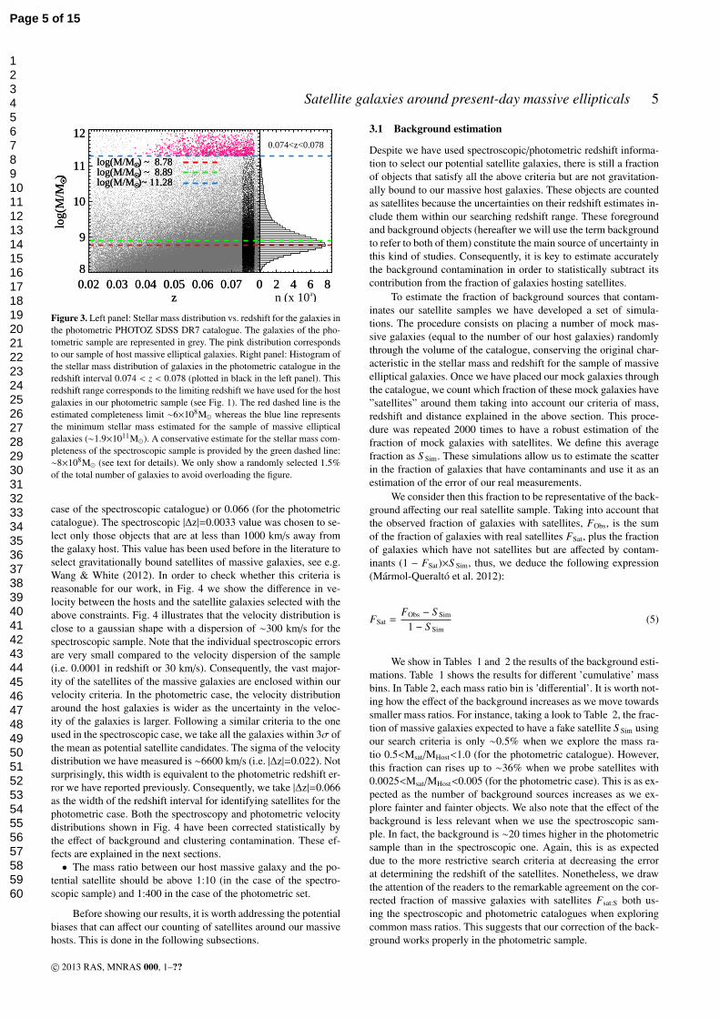
Figure 6. Panel a): Cumulative fraction of massive elliptical galaxies which

host at least one satellite as a function of the mass ratio MSat/MHost for

the photometric sample. Points plotted in red show the fraction of mas-

sive elliptical galaxies with satellites after applying the clustering correc-

tion whereas the blue points are the result of correcting by the background.

The dashed lines correspond to FObs (black), S Sim (blue) and S Clu (red)

(see Sec. 3.1 and 3.2). The black solid points correspond to the results by

Marmol-Queralto et al. (2012) for 1:10 and 1:100 mass ratios. The frac-

tion of Milky Way like galaxies with satellites obtained by Liu et al. (2011)

is represented by a green point for satellites down to a 1:10 mass ratio.

The vertical grey dashed area correspond to the mass ratio region where

incompleteness in our photometric satellite sample could play a role (see a

discussion in Sec. 2.2.2). Panel b): Average cumulative number of satellites

per galaxy host vs. the mass ratio satellite-host. Panel c): Projected average

radial distance of the satellites to their galaxy hosts. Panel d): Cumulative

multiplicity of satellites around the massive ellipticals as a function of the

mass ratio satellite-host.

c© 2013 RAS, MNRAS 000, 1–??

Page 8 of 15

123456789101112131415161718192021222324252627282930313233343536373839404142434445464748495051525354555657585960

Satellite galaxies around present-day massive ellipticals 9

using the two different catalogues. This shows the consistency of

our results using different samples.

We can now repeat the same exercise than above but show-

ing which fraction of massive ellipticals has at least one satellite

at different mass ratio bins. The bins we have chosen are shown in

Table 2 and Fig. 8. One of the most remarkable results we found

in this paper is that contrary to what we see in the case of the cu-

mulative mass ratio, when we explore the differential mass ratio,

the fraction of massive galaxies with at least one low mass (i.e.

with MSat/MHost<0.05) satellite remains almost constant (∼20%).

We will discuss the implication of this result in the discussion sec-

tion.

4.2 Properties of the population of satellite galaxies

In addition to quantify the fraction of massive elliptical galax-

ies having satellites, for each mass ratio MSat/MHost, we estimate

the average projected radial distances of these satellites to their

host DSat, the average number of satellites per galaxy host (i.e.

NSat/NHost), and the typical number of companions found around

the central objects in those cases where they have at least one satel-

lite nSat (i.e. the multiplicity). To estimate properly these quantities,

we need to correct for the effect of the contaminants. To achieve this

goal, we have carried on the following procedure. We start with the

equality:

NObs = NSat + Ncont (6)

where NObs is the observed number of satellite candidates, NSat

is the number of real satellites and Ncont is the number of galaxies

missidentified as satellites (i.e. contaminants). These fake satellites

should be represented by the typical number of contaminants found

in the simulations (Ncont ∼ NSim) already introduced in the sec-

tion 3.15. Rewriting Eq. 6 using probability distributions at a given

radial distance R (i.e. Nk(R) = Pk(R)NTotal,k) we obtain:

PSat(R)NSat = PObs(R)NObs − PSim(R)NSim (7)

We can now exemplify this technique. Let’s define the average

projected radial distance of the satellites as:

< Dk >=

∫ R

0

Pk(R′)R′ dR′ (8)

we get the following equation:

< DSat >=NObs

NObs − NSim

< DObs > −NSim

NObs − NSim

< DSim > (9)

< DSat > is the average projected radial distance of the real

satellite galaxies after the background correction. < DObs > is the

average projected radial distance measured directly in the data be-

fore the background correction and < DSim > is the average pro-

jected radial distance found in the background simulations. Other

properties such as the average mass fraction of the satellites, their

colors, etc, could be evaluated using the above expression simply

replacing the average radial distances by the average quantity that

we would like to estimate.

5 To illustrate the methodology, we refer only here to the background cor-

rection, but exactly the same procedure applies for correcting the clustering

effect by simply changing NSim by NClu.

4.2.1 Average projected radial distance satellite-host

The average projected radial distance of the satellites to the galaxy

host is a measurement about the vicinity of the satellite popula-

tion to their main galaxies. A change of this quantity with cosmic

time could be an indication of a progressive infall of the satellites

towards their host galaxies. In this work, we quantify this measure-

ment at z=0, helping future works at higher redshifts to explore

changes of this quantity with cosmic time.

The corrected average radial projected distance of the satel-

lites <DSat> are shown in Fig. 6 and 8 for the cumulative and dif-

ferential case respectively. It is worth noting that in the two cases

the average distance of the galaxies is relatively constant 58.5 kpc

(cumulative case) and 59 kpc (differential case), independently of

the explored mass ratio. This value is lower than the expected the-

oretical value for a random distribution of objects within a circle of

R=100 kpc which is 66.6 kpc. As it is shown in those Figures, the

background simulation recovers the expected theoretical value. For

the clustering correction, we have assumed the theoretical value

<DClu>=66.6 kpc since our method to assess the clustering does

not allow us to estimate such quantity directly as we analyze the

rings beyond 100 kpc. The comparison between the photometric

and the spectroscopic samples is shown in panel c) of Fig. 7. Inter-

estingly, the projected distances measured using the spectroscopic

redshift are systematically above the values using the photometric

sample. This result is likely connected with the fact that two spec-

troscopic fibers cannot be placed closer than 55′′on a given plate

in the SDSS survey. At the typical redshift of the spectroscopic

sample (z∼0.049), this distance corresponds to the following rest-

frame distance 52.7 kpc. We illustrate this observational ”hole” of

the spectroscopic sample in the upper panel of Fig. 9.

The values that we have estimated, consequently, should be

seen as upper limits of the real average radial projected distance of

the satellites. This is because we have assumed at correcting our

values that all distances, from 0 to 100 kpc can be occupied by

the satellites. In observations, however, the distribution of satellites

does not include objects within the inner ∼15-20 kpc in the pho-

tometric sample and very little up to 50 kpc in the spectroscopic

sample (see Fig. 9). In the case of the photometric sample, satel-

lites with smaller projected distances to the host galaxies have ei-

ther been cannibalized or their light could be eclipsed by the hosts.

In this sense, we will be unable to separate those objects from the

host. In the case of the spectroscopic sample, we have also added

the problem of the fiber collisions as we stated above.

How much this effect could affect our distance estimation?

We have made a crude estimation of this effect as follows. Assum-

ing that the probability distribution of the radial distribution of the

satellites P(R) is constant (see e.g. Fig. 9), we obtain:

< DSat >corr=1

1 + α< DSat > (10)

where α is the radial fraction occupied by the host galaxy com-

pared to the total search radius. In the photometric case α=0.15-0.2,

which implies that a much reliable value for <DSat> is 49-51 kpc.

In the spectroscopic case we have tentatively assume that α is 0.5,

obtaining <DSat>∼45 kpc. We will discuss this result as well as

the independence with respect to the mass ratio of the average pro-

jected radial distance of the satellites in the discussion section.

4.2.2 Average number of satellites per galaxy host

We also quantify which is the average number of satellites per

galaxy host NSat/NHost as a function of the mass ratio satellite-host.

c© 2013 RAS, MNRAS 000, 1–??

Page 9 of 15

123456789101112131415161718192021222324252627282930313233343536373839404142434445464748495051525354555657585960

10 Pablo Ruiz, Ignacio Trujillo & Esther Marmol-Queralto

We show this in Figs. 6 and 8. These values have been corrected

of the effect of background and clustering. We have done this by

subtracting to NObs the typical number of contaminants NSim and

NClu found in the background simulation and in our estimates of

clustering respectively.

According to Fig. 6 there is only ∼0.25 satellites per mas-

sive elliptical if we explore satellites down to a mass ratio 1:10.

However, this number grows up to ∼1 satellite per massive host if

we explore satellites down to a mass ratio 1:100. That means that,

on average, almost all massive ellipticals (i.e. with a M&1011M⊙)

have a companion with a mass larger than M&109M⊙. This num-

ber, however, does not seem to grow fast (i.e. exponentially) when

we explore even lower mass satellites. This is well seen in Fig. 8.

We see that for satellites less massive than M.1010M⊙, the average

number of satellites per galaxy host in each mass ratio bin is almost

constant. That means that the cumulative number of satellites as

we decrease in stellar mass only grows approximately linearly with

logM of the satellites.

4.2.3 Multiplicity around the massive elliptical galaxies

To end this section about the properties of the satellite distribution

around massive ellipticals, we explore the multiplicity nSat of satel-

lites around our massive hosts. In other words, we probe which is

the typical number of satellites in those cases where there is at least

one satellite found.

Our findings are shown again in Figs. 6 and 8 for the cu-

mulative and the differential case. For the differential case, our re-

sults indicate that at every mass bin (i.e. Fig. 8), there is only a

small probability of finding more than one satellite within the same

mass ratio. That means that once we have fixed the stellar mass

of the satellite, the probability of finding another one surrounding

the massive elliptical with a similar mass is very low. This is in-

dependent of the mass bin explored and does not increase towards

satellites less and less massive. Consequently, when we explore the

cumulative multiplicity nSat (i.e. Fig. 6), we only see a moderate

increase towards larger and larger mass ratios. For instance, to get

a cumulative multiplicity larger than 2, we need to considerably

decrease the stellar mass of the satellites probed (i.e. we need to

explore satellites at least down to a mass of M⋆∼109M⊙).

5 THE MERGING CHANNEL OF MASSIVE

ELLIPTICALS

We now explore a more speculative aspect of our work. Eventually,

some satellites surrounding our massive ellipticals will infall into

their massive hosts. Consequently, we can estimate which are the

properties of the satellites that could contribute most to a potential

mass growth of the host galaxies in the future. On what follows, we

assume that all satellites, independently of their mass, will infall

with the same speed towards the central galaxy. Note, however, that

this could be not necessary true, as it is theoretically expected that

larger the mass of the satellite shorter will be its merging timescale

(Jiang et al. 2013).

To probe the most likely merging channel what we have done

is the following. We have estimated all the stellar mass that is con-

tained by the satellites of a given mass ratio in our sample and we

have divided this quantity by the sum of the mass of all the host

galaxies. In other words, we have calculated the following quan-

tity:

Ψ =

NSat−bin∑

i=1

MSat−bin,i

NHost∑

j=1

MHost,j

(11)

The sum of all the mass in the host galaxies is a fixed quan-

tity for our samples and their values are∑NHost

j=1MHost,j=1.8×1014M⊙

(spectroscopic sample) and∑NHost

j=1MHost,j=4.1×1014M⊙ (photomet-

ric sample).

In Fig. 10 and Table 3, we show the most likely merging

channel of our massive ellipticals. We show our results after be-

ing corrected by the effect of the background and clustering. We

have assumed poissonian errors to estimate our error bars. The to-

tal amount of mass contained in the satellite population down to

1:10 compared to the total amount of mass in the hosts is ∼6%

(using the spectroscopic sample) or ∼5.5% (using the photometric

sample). Down to 1:400 this value is ∼8% of the total amount of

mass contained in their hosts. The largest contributor to the satellite

mass are those satellites with a mass ratio from 1:2 to 1:5 (∼28%

of the total mass of the satellites in the photometric sample). If the

satellites eventually infall into the host galaxies, the merger chan-

nel will be largely dominated by satellites with a mass ratio be-

low 1:10 (which have 68% of the total mass in satellites). This is

again a result of the approximately constant number of satellites

we find when we move towards less and less massive satellites. For

this reason, the decrease of the stellar mass in the satellites can not

be compensated by a larger number of these objects and the main

driver of mass accretion is provided by the larger satellites. If the

theoretical expectation holds and the merger timescales are shorter

for the most massive satellites, the mass growth due to the larger

satellites will be even more important than the result show in Fig.

10. We discuss the consequence of this result in the next section.

6 DISCUSSION

The results presented in this paper can be used as a z∼0 reference

for the study of the evolution of satellites around massive elliptical

galaxies with cosmic time. As we mentioned in the Introduction,

several studies have addressed recently the evolution of the num-

ber of satellites of massive ellipticals with redshift both observa-

tionally and theoretically. These previous studies have shown that

the fraction of massive elliptical galaxies with satellites of a given

mass ratio has remained constant since at least z∼2. However, those

works disagree on the number of massive galaxies having satellites,

being more abundant the satellites in the simulations than in the ob-

servations. In this paper, which is less affected by incompleteness

at small stellar masses than previous works, we can readdress this

question and see how the theoretical expectations compare to the

observational data in the nearby universe.

6.1 Comparison with theoretical expectations

Quilis & Trujillo (2012) have estimated, using the Millennium sim-

ulation, what is the expected fraction of massive galaxies having

satellites with a mass ratio down to 1:10 and down to 1:100 within

a sphere of R=100 kpc. They have conducted such studies explor-

ing galaxies from z=2 to now using three different semianalytical

models. At z=0, the theoretical expectations suggest that the frac-

tion of massive galaxies having satellites with mass ratio down to

1:10 ranges from 0.3 to 0.4. Observationally, we have found 0.23

c© 2013 RAS, MNRAS 000, 1–??

Page 10 of 15

123456789101112131415161718192021222324252627282930313233343536373839404142434445464748495051525354555657585960

Satellite galaxies around present-day massive ellipticals 11

Table 3. The merging channel of present-day massive ellipticals. The table shows the contribution of the satellite mass enclosed in each satellite mass bin to

the total mass confined in their hosts. We show the observed fraction (in %) and the fractions (in %) after correcting of background and clustering.

MSat/MHost Ψ (Obs) Ψ (Sim) Ψ (Clu)

Spectroscopic sample

0.5-1.0 1.67 ± 0.33 1.67 ± 0.32 1.40 ± 0.31

0.2-0.5 2.68 ± 0.27 2.64 ± 0.27 2.08 ± 0.24

0.1-0.2 2.39 ± 0.19 2.37 ± 0.18 2.07 ± 0.17

Total 6.77 ± 0.47 6.68 ± 0.46 5.55 ± 0.42

Photometric sample

0.5000-1.000 2.42 ± 0.35 2.02 ± 0.33 1.64 ± 0.29

0.2000-0.500 3.14 ± 0.27 2.46 ± 0.24 2.00 ± 0.21

0.1000-0.200 1.97 ± 0.15 1.50 ± 0.13 1.26 ± 0.12

0.0500-0.100 1.51 ± 0.09 1.15 ± 0.08 0.93 ± 0.07

0.0200-0.050 1.30 ± 0.06 0.95 ± 0.05 0.82 ± 0.05

0.0100-0.020 0.62 ± 0.03 0.37 ± 0.02 0.34 ± 0.02

0.0050-0.010 0.41 ± 0.02 0.20 ± 0.01 0.17 ± 0.01

0.0025-0.005 0.24 ± 0.01 0.09 ± 0.01 0.08 ± 0.01

Total 11.59 ± 0.48 8.75 ± 0.44 7.21 ± 0.39

after the background correction and 0.20 after the clustering correc-

tion (using the spectroscopic sample). These values are lower than

the theoretical expectations. If we focus our attention now towards

satellites with lower masses, we find that the theoretical expected

fraction of massive galaxies with at least a satellite with a mass ratio

down to 1:100 is between 0.6 and 0.7. These values are again larger

than the observed data, where we find 0.52 after the background

correction and 0.45 after the clustering correction (using the pho-

tometric sample). It is worth stressing that this discrepancy among

the theoretical and the observational results can not be explained

due to the different volumes of exploration used in both works: a

spatial sphere of 100 kpc in Quilis & Trujillo (2012) and a cylinder

in redshift here. Due to the way we have selected our galaxies in

redshift (using up to 3 sigma away from the redshift of the galaxy

host), basically all the satellite galaxies in the line of sight of the

host within a projected radial distance of 100 kpc are taken. In that

sense, at comparing with the Millenium simulation our number of

observed satellites should be an upper limit (as they are only re-

stricted to 100 kpc in depth). As the number of theoretical satellites

is larger than observed, we can confidently claim that there is a

discrepancy with our observations. Also note that the inner hole in

the number of observed satellites produced by the presence of the

galaxy host (see Fig. 9) only outshone a small fraction of the probed

area (∼4% for the photometric sample). Consequently, this can not

help to explain the discrepancy either. Finally, a potential lost of

satellites in the work by Quilis & Trujillo (2012) due to resolution

effects will also increase the discrepancy between the simulations

and the observations.

We think that the excess of satellites found in the Millenium

simulation is due to the inability of the semianalytical models to

reproduce (see the Fig. 20 of Guo et al. 2011) the right cluster-

ing of low mass (M⋆<6×1010M⊙) galaxies at small scales (R<1

Mpc). The model substantially overproduce the clustering at small

scales for these low mass objects. Guo et al. (2011) suggest that

this discrepancy could be due to the large σ8=0.9 adopted in the

simulation compared to the observational most likely value of

σ8=0.834±0.027 (Planck Collaboration et al. 2013).

Another quantity that we can compare with the theoretical pre-

dictions is the average projected radial distance of the satellites to

their galaxy hosts. Quilis & Trujillo (2012) found that the aver-

age projected radial distance ranges within 35 to 45 kpc. Here we

find a value which is ∼59 kpc and that could be decreased down

to 49-51 kpc if the incompleteness of satellites in the central re-

gion of search is accounted for. It is worth noting that in our rough

correction of the incompleteness, we have assumed an equal prob-

ability with the radius of the satellite distribution. In practice, it is

likely that there would be an excess of probability of finding more

satellites closer to the galaxy hosts than what we have assumed. If

this were the case, our estimation of a projected (corrected) radial

distance of ∼50 kpc would be an upper limit. Moreover, we warn

the reader that a direct comparison among the theoretical and ob-

servational results is not straightforward. Quilis & Trujillo (2012)

search for satellites within a sphere of R=100 kpc whereas the ob-

servational search actually resembles a cylinder. In this sense, the

observed radial distance can be again more prone towards larger ra-

dial distances than the theoretical study. Summarizing, the average

radial distance of the satellites in the simulation and in the obser-

vations, once the incompleteness in the observations are accounted

for, could be in reasonable agreement.

6.2 Comparison with previous data

We can now draw our attention to the fraction of massive galaxies

with satellites found in other works at z=0. Liu et al. (2011), ex-

ploring MW-like galaxies (i.e. objects which are less massive than

our host galaxies), found that only 14% of those objects have at

least a satellite within R=100 kpc down to 1:10 mass ratio (private

communication). In Fig. 6 we have compared this observation with

our results. Liu’s number is slightly below our findings (20-23% in

the spectroscopic sample) but we think it is as expected taking into

account that the number of satellites depends on the mass and the

color of the host (Wang & White 2012). Larger the mass of the host

larger is the number of its satellites.

A more direct comparison with our range of mass for the host

galaxies can be done with the results of Wang & White (2012).

In that work, the authors have not segregated the galaxies using

c© 2013 RAS, MNRAS 000, 1–??

Page 11 of 15

123456789101112131415161718192021222324252627282930313233343536373839404142434445464748495051525354555657585960

12 Pablo Ruiz, Ignacio Trujillo & Esther Marmol-Queralto

visual morphology but colors. We will compare our results with

the ones found for their red hosts, likely the most similar to our

elliptical galaxies. Another important difference is that they have

done the search of satellites within a radius of 300 kpc. Conse-

quently, to allow a direct confrontation with this dataset we have

repeated our analysis using such radius and only for those host

galaxies with 11.1<logM⋆<11.4 (their green line in their Fig. 7).

We get the following results: a) for satellites with logM⋆=10,

NSat/NHost/ log M⋆=3.2-4.5 (ours) and 3-4 (Wang & White) and b)

for satellites with logM⋆=9, NSat/NHost/ log M⋆=4.5-6.1 (ours) and

6-7 (Wang & White). This agreement is remarkable taking into ac-

count the different techniques and selection of the galaxy hosts.

Finally, we can make a comparison with Marmol-Queralto et

al. (2012). These authors conducted a similar analysis to what we

have done here but for galaxies at higher redshifts (0.2<z<2). We

compare our numbers (see Fig. 6) with the galaxies they classi-

fied as ellipticals in their lower redshift range (0.2<z<0.75). They

found that the fraction of massive galaxies with satellites down to

1:10 is 0.23-0.28. Here we find 0.20-0.24 (in the spectroscopic sam-

ple depending whether the clustering or background correction has

been applied) and 0.16-0.19 (in the photometric sample), which

is slightly below but in reasonable agreement with those results.

Summarizing, our results seem to agree pretty well with previous

studies in those ranges of masses where a direct comparison can be

conducted.

6.3 The merging channel in the present-day universe

There is currently a strong debate about what is the favored merg-

ing channel which explains the dramatic increase in size of the mas-

sive galaxies in the last 11 Gyr. Whereas there is a growing agree-

ment (see e.g. Trujillo et al. 2011) that the size evolution can not be

entirely explained by internal mechanisms like AGN activity (Fan

et al. 2008, 2010; Ragone-Figueroa & Granato 2011), it is not clear

what is the relevance of major versus minor merging in the growth

of the galaxies. On one hand, major mergers (e.g. Ciotti & van Al-

bada 2001; Nipoti, Londrillo, & Ciotti 2003; Boylan-Kolchin, Ma,

& Quataert 2006; Naab et al. 2007) seem to be very scarce (at least

since z∼1; Bundy et al. 2009; deRavel et al. 2009; Wild et al. 2009;

Lopez-Sanjuan et al. 2010; Kaviraj et al. 2011) to play a major role

in the growth of the galaxies. On the other hand, minor merging

(favoured theoretically for its efficiency on increasing the size of

the galaxies; Khochfar & Burkert 2006; Maller et al. 2006; Hop-

kins et al. 2009b; Naab et al. 2009) confronts some problems with

the number of satellites found at z∼1 (e.g. Ferreras et al. 2013).

Oser et al. (2012) have suggested that the most likely scenario

is an increase in size and mass of the massive galaxies through

satellites having a mass ratio of 1:5. The results of our paper can

not solve this question directly, as we would need to explore the

satellite distribution at different cosmic times to address this issue.

However, motivated by the observed (Marmol-Queralto et al. 2012)

and theoretically expected (Quilis & Trujillo 2012) constancy of

the fraction of massive galaxies having satellites since z=2, we can

speculate about the merging channel of massive ellipticals back in

time.

If galaxies at high-z would follow the same mass distribution

than the one observed in the nearby universe, then the observations

will suggest that the mass and size increase of the massive elliptical

galaxies will be dominated by satellites with mass ratio within 1:2

to 1:5 (see also Lopez-Sanjuan et al. 2012). Note, however, that

this statement assumes that the merger timescale are independent

on the mass ratio between the satellites and the host galaxies. More

realistic scenarios (e.g. Jiang et al. 2013) suggest that the merger

timescale rises as the mass ratio between both galaxies increases.

In this sense, the smaller satellites will take significantly more time

to merge with the host galaxies than the bigger satellites. Based

on this, what we can claim with some confidence is that low mass

satellites with mass ratio below 1:10 would play a minor role in the

mass increase of the host galaxies. They would be just very small

in number to contribute to the mass growth plus they will have very

large timescales to efficiently infall into the massive ellipticals.

7 SUMMARY AND CONCLUSIONS

In this paper we have explored the properties of the satellite popu-

lation around massive, visually classified, ellipticals in the nearby

Universe (z<0.1). Our aim has been to robustly quantify the dis-

tribution of satellites around this type of objects to create a local

reference for future studies of the evolution of the satellites with

cosmic time. We have based our analysis on a sample of ∼1000

massive ellipticals obtained from the catalogue of Nair & Abraham

(2010). To explore the satellite distribution around these objects we

used the spectroscopic NYU Value-Added Galaxy Catalogue and

the photometric PHOTOZ SDSS DR7 catalogue. This has allowed

us to explore satellites down to a mass ratio of 1:400.

Our satellite galaxies have been identified within a projected

radial distance of 100 kpc around the hosts. A careful analysis of

the background and clustering contamination has been done. We

have found that only 20-23% of the massive ellipticals has at least

one satellite with a mass ratio down to 1:10. This number increases

to 45-52% if we explore satellites down to 1:100 and to >60-70%

if we go down to 1:400. The average observed projected radial dis-

tance of the satellites to the host is ∼59 kpc (which can be decreased

down to, at least, ∼50 kpc if we account for incompleteness ef-

fects). The observed number of satellites are lower than the pre-

dictions from theoretical expectations (see e.g. Quilis & Trujillo

2012). It will be worth exploring in the future whether this dis-

agreement with the theoretical models increases for satellites with

lower masses (i.e. M∗.108M⊙).

Finally, the number of satellites per galaxy host only increases

very mildly at decreasing the satellite mass. The fraction of mass

which is contained in the satellites down to a mass ratio of 1:400

is ∼8% of the total mass contained by the hosts. The largest con-

tributor to the mass enclosed by the satellites are those satellites

with a mass ratio from 1:2 to 1:5 (in fact, ∼28% of the total mass

of the satellites is within objects with such mass ratio). If the satel-

lites eventually infall into the host galaxies, the merger channel will

be largely dominated by satellites with a mass ratio down to 1:10

(these satellites have 68% of the total mass in satellites). Futures

studies (see, for instance, Ferreras et al. 2013), exploring how is the

mass distributed among the satellites of higher redshift objects, will

allow to test whether the currently suggested most likely scenario

for explaining the increase in size and mass of the massive galaxies

(i.e. by the infall of satellites having a mass ratio of around 1:5;

Oser et al. 2012) is favored or not.

ACKNOWLEDGMENTS

We thank the referee for his/her constructive comments and care-

ful reading of our manuscript. We are grateful to Juan Betancort

for his help on the statistical analysis conducted in this paper. Vi-

cent Quilis and Thorsten Naab help to understand better the com-

c© 2013 RAS, MNRAS 000, 1–??

Page 12 of 15

123456789101112131415161718192021222324252627282930313233343536373839404142434445464748495051525354555657585960

Satellite galaxies around present-day massive ellipticals 13

parison between the theoretical and observational results. Carlos

Lopez Sanjuan did some interesting observations on the back-

ground corrections applied to the data. This work has been sup-

ported by the “Programa Nacional de Astronomıa y Astrofısica”

of the Spanish Ministry of Science and Innovation under grant

AYA2010-21322-C03-02. EMQ acknowledges the support of the

European Research Council via the award of a Consolidator Grant

(PI McLure). This project has made use of data from the Sloan

Digital Sky Survey (SDSS). Funding for the SDSS has been pro-

vided by the Alfred P. Sloan Foundation, the Participating Insti-

tutions, the National Science Foundation, the U.S. Department

of Energy, the National Aeronautics and Space Administration,

the Japanese Monbukagakusho, the Max Planck Society, and the

Higher Education Funding Council for England. The SDSS Web

Site is http://www.sdss.org/.

The SDSS is managed by the Astrophysical Research Con-

sortium for the Participating Institutions. The Participating Institu-

tions are the American Museum of Natural History, Astrophysical

Institute Potsdam, University of Basel, University of Cambridge,

Case Western Reserve University, University of Chicago, Drexel

University, Fermilab, the Institute for Advanced Study, the Japan

Participation Group, Johns Hopkins University, the Joint Institute

for Nuclear Astrophysics, the Kavli Institute for Particle Astro-

physics and Cosmology, the Korean Scientist Group, the Chinese

Academy of Sciences (LAMOST), Los Alamos National Labora-

tory, the Max-Planck-Institute for Astronomy (MPIA), the Max-

Planck-Institute for Astrophysics (MPA), New Mexico State Uni-

versity, Ohio State University, University of Pittsburgh, University

of Portsmouth, Princeton University, the United States Naval Ob-

servatory, and the University of Washington.

REFERENCES

Abazajian K., et al., 2009, ApJS, 182, 543

Adelman-McCarthy J. K., et al., 2006, ApJS, 162, 38

Bailin J., Power C., Norberg P., Zaritsky D., Gibson B. K., 2008,

MNRAS, 390, 1133

Bezanson R., van Dokkum P. G., et al., 2009, ApJ, 697, 1290

Bell E. F., McIntosh D. H.,et al., 2003, ApJS, 149, 289

Blanton M. R., et al., 2005, AJ, 129, 2562

Blanton M. R., Roweis S., 2007, AJ, 133, 734

Bournaud, F., Chapon, D., Teyssier, R., et al. 2011, ApJ, 730, 4

Boylan-Kolchin M., Ma C.-P., Quataert E., 2006, MNRAS, 369,

1081

Buitrago F., Trujillo I., et al., 2008, ApJL, 687, L61

Bundy K., Fukugita M., Ellis R. S., Targett T. A., Belli S., Kodama

T., 2009, ApJ, 697, 1369

Cenarro A. J., Trujillo I., 2009, ApJ, 696, L43

Chen J., Kravtsov A. V., et al., 2006, MNRAS, 381, 962

Ciotti L., van Albada T. S., 2001, ApJ, 552, L13

Dekel, A., Birnboim, Y., Engel, G., et al. 2009, Nature, 457, 451

DeLucia G., Blaizot J.,et al., 2007, MNRAS, 375, 2

Dıaz-Garcıa, L. A., Marmol-Queralto, E., Trujillo, I., et al. 2013,

MNRAS, 433, 60

de Ravel L., Le Fevre O.,et al., 2009, A&A, 498, 379

Fan L., Lapi A., et al., 2010, ApJ, 718, 1460

Fan L., Lapi A., et al., 2008, ApJL, 689, L101

Feldmann, R., Carollo, C. M., & Mayer, L. 2011, ApJ, 736, 88

Ferreras I., et al., 2013, MNRAS, submitted, arXiv:1312.5317

Guo Q., White S., et al., 2011, MNRAS, 412, 101

Holmberg E., 1969, Arkiv for Astronomi, 5, 305

Hopkins, P. F., Bundy, K., Murray, N., et al. 2009a, MNRAS, 398,

898

Hopkins P. F., Hernquist L., et al., 2009b, ApJ, 691, 1424

Huertas-Company M., Shankar F., Mei S., Bernardi M., Aguerri

J. A. L., Meert A., Vikram V., 2013, ApJ, 779, 29

Jackson, N., Bryan, S. E., Mao, S., & Li, C. 2010, MNRAS, 403,

826

Jiang, C., Jing, Y., & Han, J. 2013, arXiv:1307.3322

Kauffmann, G., Heckman, T. M., White, S. D. M., et al. 2003,

MNRAS, 341, 33

Kaviraj S., Tan K.-M., Ellis R. S., Silk J., 2011, MNRAS, 411,

2148

Keres, D., Katz, N., Weinberg, D. H., & Dave, R. 2005, MNRAS,

363, 2

Khochfar, S., & Silk, J. 2006, ApJ, 648, L21

Khochfar S., Burkert A., 2006, AJ, 445, 403

Kroupa P.,2001, MNRAS, 322, 231

Liu L., Gerke B. F., et al., 2011, ApJ, 733, 62

Lopez-Sanjuan C., Ballcels M., et al., 2010, ApJ, 710, 1170

Lopez-Sanjuan C., et al., 2012, A&A, 548, A7

Maller A. H., Katz N., Keres D., Dave R., Weinberg D. H., 2006,

ApJ, 647, 763

Man A. W. S., Toft S., et al., 2012, ApJ, 744, 85

Marmol-Queralto, E., Trujillo, I., Perez-Gonzalez, P. G., Varela,

J., & Barro, G. 2012, MNRAS, 422, 2187

Marmol-Queralto, E., Trujillo, I., Villar, V., Barro, G., & Perez-

Gonzalez, P. G. 2013, MNRAS, 429, 792

Naab T., Johansson P. H., Ostriker J. P., Efstathiou G., 2007, ApJ,

658, 710

Naab T., Johansson P. H., Ostriker J. P., 2009, ApJ, 699, L178

Nair P. B., Abraham R. G., 2010, AJS, 186, 427

Newman A. B., Ellis R. S., et al., 2012, ApJ, 746, 162

Nierenberg A. M., Auger M. W., et al., 2011, ApJ, 731, 44

Nierenberg A. M., Treu T., Menci N., Lu Y., Wang W., 2013, ApJ,

772, 146

Nipoti C., Londrillo P., Ciotti L., 2003, MNRAS, 342, 501

Oser, L., Ostriker, J. P., Naab, T., Johansson, P. H., & Burkert, A.

2010, ApJ, 725, 2312

Oser L., Naab T., et al., 2012, ApJ, 744, 63

Planck Collaboration, et al., 2013, arXiv:1303.5076

Ragone-Figueroa, C., & Granato, G. L. 2011, MNRAS, 414, 3690

Ricciardelli, E., Trujillo, I., Buitrago, F., & Conselice, C. J. 2010,

MNRAS, 406, 230

Ricciardelli E., Vazdekis A., Cenarro, A.J. et al., 2012, MNRAS,

424, 172R

Sales L., Lambas D. G., 2004, MNRAS, 348, 1236

Sales L., Lambas D. G., 2005, MNRAS, 356, 1045

Schlegel, D. J., Finkbeiner, D. P., & Davis, M. 1998, ApJ, 500,

525

Trujillo I., Conselice C. J., et al., 2007, MNRAS, 382, 109

Trujillo, Ferreras, de La Rosa, 2011, MNRAS, 938, 3903

van Dokkum, P. G., Whitaker, K. E., Brammer, G., et al. 2010,

ApJ, 709, 1018

Vazdekis A., Ricciardelli E., Cenarro A. J. et al., 2012, MNRAS,

424, 157V

Quilis V. & Trujillo I., 2012, ApJ, 752, L19

Wang, W., & White, S. D. M. 2012, MNRAS, 424, 2574

White S. D. M. & Rees M. J., 1978, MNRAS, 183, 341W

Wild V., Walcher C. J., Johansson P. H., Tresse L., Charlot S.,

Pollo A., Le Fevre O., de Ravel L., 2009, MNRAS, 395, 144

Wuyts, S., Cox, T. J., Hayward, C. C., et al. 2010, ApJ, 722, 1666

c© 2013 RAS, MNRAS 000, 1–??

Page 13 of 15

123456789101112131415161718192021222324252627282930313233343536373839404142434445464748495051525354555657585960

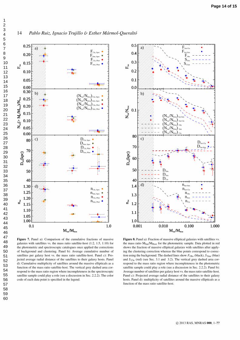
14 Pablo Ruiz, Ignacio Trujillo & Esther Marmol-Queralto

0.00

0.05

0.10

0.15

0.20

0.25

F Sat

0.00

0.05

0.10

0.15

0.20

0.25

F Sat

a)FClu, Spec

FSim, Spec

FClu, Phot

FSim, Phot

0.00

0.05

0.10

0.15

0.20

0.25

0.30

NSa

t(> M

Sat/M

Hos

t)/N

Hos

t

0.00

0.05

0.10

0.15

0.20

0.25

0.30

NSa

t(> M

Sat/M

Hos

t)/N

Hos

t

b)(NSat/NHost) Clu, Spec

(NSat/NHost) Sim, Spec

(NSat/NHost) Clu, Phot

(NSat/NHost) Sim, Phot

40

50

60

70

80

DSa

t(kpc

)

40

50

60

70

80

DSa

t(kpc

)

c) DClu, Spec

DSim, Spec

DClu, Phot

DSim, Phot

0.1 1.0MSat/MHost

1.001.05

1.10

1.15

1.20

1.25

1.30

n Sat

0.1 1.0MSat/MHost

1.001.05

1.10

1.15

1.20

1.25

1.30

n Sat

d) nClu, Spec

nSim, Spec

nClu, Phot

nSim, Phot

Figure 7. Panel a): Comparison of the cumulative fractions of massive

galaxies with satellites vs. the mass ratio satellite-host (1:2, 1:5, 1:10) for

the photometric and spectroscopic catalogues once applied the corrections

of background and clustering. Panel b): Average cumulative number of

satellites per galaxy host vs. the mass ratio satellite-host. Panel c): Pro-

jected average radial distance of the satellites to their galaxy hosts. Panel

d): Cumulative multiplicity of satellites around the massive ellipticals as a

function of the mass ratio satellite-host. The vertical grey dashed area cor-

respond to the mass ratio region where incompleteness in the spectroscopic

satellite sample could play a role (see a discussion in Sec. 2.2.2). The color

code of each data point is specified in the legend.

0.0

0.1

0.2

0.3

0.4

0.5

F Sat

a)

0.0

0.1

0.2

0.3

0.4

0.5

F Sat

FSat-Clu

FSat-Sim

FObs

SSim

SClust

0.1

NSa

t/NH

ost

0.1

NSa

t/NH

ost

b)

(NSat/NHost) Clu

(NSat/NHost) Sim

(NSat/NHost) Obs

(NSat/NHost) Sat-Clu

(NSat/NHost) Sat-Sim

40

50

60

70

80

DSa

t(kpc

)

c)

40

50

60

70

80

DSa

t(kpc

)

DSat-Clu

DSat-Sim

DClu

DSim

DObs

0.001 0.010 0.100 1.000MSat/MHost

1.0

1.1

1.2

1.3

1.4

n Sat

d)

0.001 0.010 0.100 1.000MSat/MHost

1.0

1.1

1.2

1.3

1.4

n Sat

nSat-Sim

nSat-Clu

nObs

nSim

nClu

Figure 8. Panel a): Fraction of massive elliptical galaxies with satellites vs.

the mass ratio MSat/MHost for the photometric sample. Data plotted in red

shows the fraction of massive elliptical galaxies with satellites after apply-

ing the clustering correction whereas the blue points correspond to correc-

tion using the background. The dashed lines show FObs (black), S Sim (blue)

and S Clu (red) (see Sec. 3.1 and 3.2). The vertical grey dashed area cor-

respond to the mass ratio region where incompleteness in the photometric

satellite sample could play a role (see a discussion in Sec. 2.2.2). Panel b):

Average number of satellites per galaxy host vs. the mass ratio satellite-host.

Panel c): Projected average radial distance of the satellites to their galaxy

hosts. Panel d): multiplicity of satellites around the massive ellipticals as a

function of the mass ratio satellite-host.

c© 2013 RAS, MNRAS 000, 1–??

Page 14 of 15

123456789101112131415161718192021222324252627282930313233343536373839404142434445464748495051525354555657585960

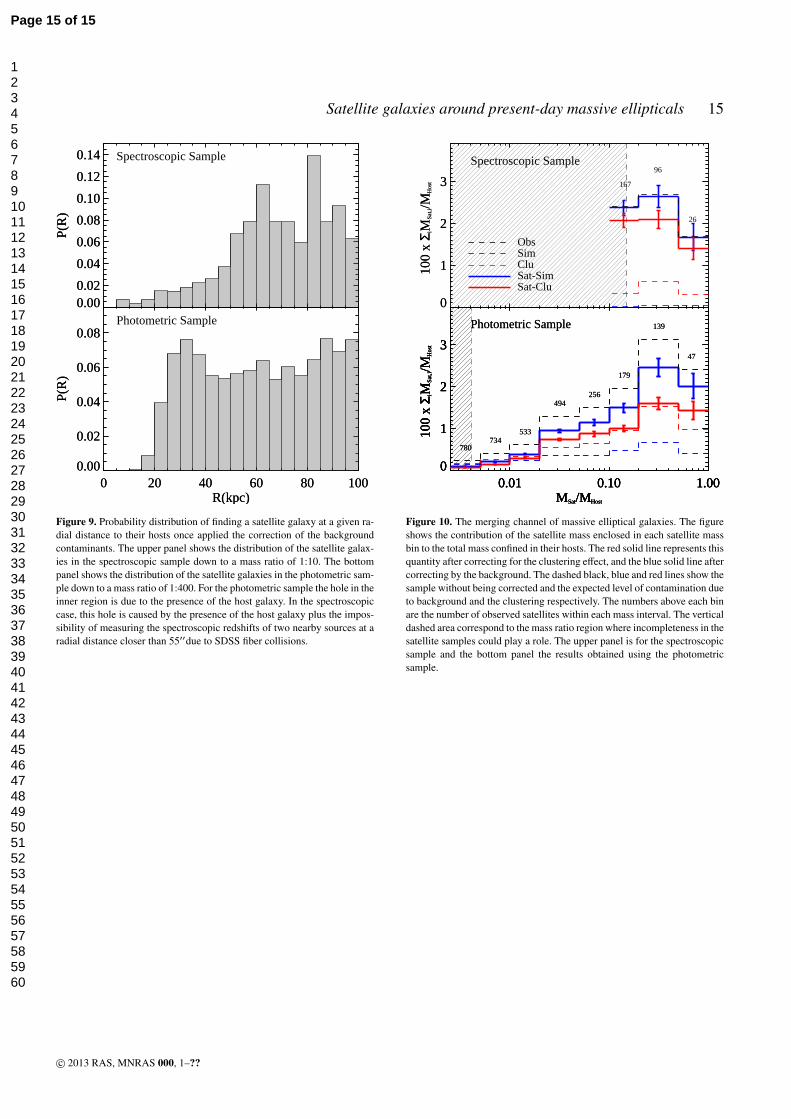
Satellite galaxies around present-day massive ellipticals 15

0.000.02

0.04

0.06

0.08

0.10

0.12

0.14

P(R

)

Spectroscopic Sample

0.000.02

0.04

0.06

0.08

0.10

0.12

0.14

P(R

)

0 20 40 60 80 100R(kpc)

0.00

0.02

0.04

0.06

0.08

P(R

)

Photometric Sample

0 20 40 60 80 100R(kpc)

0.00

0.02

0.04

0.06

0.08

P(R

)

Figure 9. Probability distribution of finding a satellite galaxy at a given ra-

dial distance to their hosts once applied the correction of the background

contaminants. The upper panel shows the distribution of the satellite galax-

ies in the spectroscopic sample down to a mass ratio of 1:10. The bottom

panel shows the distribution of the satellite galaxies in the photometric sam-

ple down to a mass ratio of 1:400. For the photometric sample the hole in the

inner region is due to the presence of the host galaxy. In the spectroscopic

case, this hole is caused by the presence of the host galaxy plus the impos-

sibility of measuring the spectroscopic redshifts of two nearby sources at a

radial distance closer than 55′′due to SDSS fiber collisions.

0

1

2

3

100

x Σ i

MSa

t,i/M

Hos

t

0

1

2

3

100

x Σ i

MSa

t,i/M

Hos

t

Spectroscopic Sample

26

96

167

Sat-CluSat-SimCluSimObs

0.01 0.10 1.00MSat/MHost

0

1

2

3

100

x Σ i

MSa

t,i/M

Hos

t

0.01 0.10 1.00MSat/MHost

0

1

2

3

100

x Σ i

MSa

t,i/M

Hos

t

Photometric Sample

47

139

179

256494

533734

780

0.01 0.10 1.00MSat/MHost

0

1

2

3

100

x Σ i

MSa

t,i/M

Hos

t

0.01 0.10 1.00MSat/MHost

0

1

2

3

100

x Σ i

MSa

t,i/M

Hos

t

Photometric Sample

47

139

179

256494

533734

780

Figure 10. The merging channel of massive elliptical galaxies. The figure

shows the contribution of the satellite mass enclosed in each satellite mass

bin to the total mass confined in their hosts. The red solid line represents this

quantity after correcting for the clustering effect, and the blue solid line after

correcting by the background. The dashed black, blue and red lines show the

sample without being corrected and the expected level of contamination due

to background and the clustering respectively. The numbers above each bin

are the number of observed satellites within each mass interval. The vertical

dashed area correspond to the mass ratio region where incompleteness in the

satellite samples could play a role. The upper panel is for the spectroscopic

sample and the bottom panel the results obtained using the photometric

sample.

c© 2013 RAS, MNRAS 000, 1–??

Page 15 of 15

123456789101112131415161718192021222324252627282930313233343536373839404142434445464748495051525354555657585960