1

Hydraulic Transients in Pump-Rising Main Systems with Quasi-constant Back Pressure

João N. Delgado1; Dídia I. C. Covas

2; and António B. de Almeida

3

ABSTRACT

The current paper aims to discuss the influence of the back pressure effect in hydraulic

transients in pumping systems caused by the sudden pump stoppage due to power failure. A

one-dimensional hydraulic transient solver was developed based on the classic water hammer

theory and solved using the Method of Characteristics. The solver incorporates the pump-

element described by Sutter parameters, the check-valve in the discharge line simulated by

the orifice law as a function of the valve opening, the pressurized surge tank described by the

polytropic process and a formulation to describe the unsteady-state friction losses. The model

was tested using transient pressure data collected from one laboratory hydraulic circuit.

Transients were generated by the sudden stoppage of the pump due to failure of the power

grid with and with the consideration of a quasi-constant backpressure. Collected data were

compared with the results of the numerical modelling and used to calibrate model parameters,

and a good agreement was obtained. The tests with the quasi-constant backpressure led to

extremely high pressure surges.

INTRODUCTION

The control of hydraulic transients in pressurized pipes is a major concern for

engineers and pipe system managers, for reasons related to risk, safety and efficient

operation. This phenomenon is caused by disturbances in flow regulation devices, such as

valves or pumps. One example of a severe disturbance in pump-raising mains is the sudden

stoppage of the pumps due to the failure of the power grid, which can lead to sub-

1 Research Fellow, Dept. of Civil Engineering, Instituto Superior Técnico, Universdade de Lisboa, Ave. Rovisco Pais, 1049-001

Lisbon, Portugal. E-mail: joao.borga.delgado@ist.utl.pt 2 Associate Professor, Dept. of Civil Engineering, Instituto Superior Técnico, Universidade de Lisboa, Ave. Rovisco Pais, 1049-001

Lisbon, Portugal. E-mail: didia.covas@tecnico.ulisboa.pt 3 Emeritus Professor, Dept. of Civil Engineering, Instituto Superior Técnico, Universidade de Lisboa, Ave. Rovisco Pais, 1049-001

Lisbon, Portugal. E-mail: betamio.almeida@.ist.utl.pt

2

atmospheric pressures or extreme overpressures. As the first one can lead to the occurrence of

cavitation or liquid column separation (Bergant et al., 2006), the latter can jeopardize the

safety of the pipe systems if the maximum pressure overcome the maximum pressure the

pipeline can withstand. One phenomenon that may induce extreme overpressures is the check

valve slam, which can be defined by the occurrence of extreme overpressures caused by the

delayed closure of the check valve when the flow reverses through this device (Thorley,

1991). According to Provoost (1983) and Thorley (1983), the higher the fluid deceleration,

the higher the pressure variation induced for the same check valve. The fluid deceleration is

related with the head difference between upstream and downstream the check valve: the

higher the head difference, the higher the fluid deceleration. Accordingly, pipe systems that

are more susceptible to check valve slam are those in which a back pressure continues to exist

after the sudden pump stoppage, such as in parallel pumping groups where only one pump

sudden stops.

The current paper aims at the experimental and numerical analysis of the pipe flow

behavior during transient events in pump-raising mains with and without the influence of the

back pressure conditions. The paper includes a brief description of the developed hydraulic

transient solver, the description of the experimental facility, the set of experimental tests

carried out and the data collected, as well as the comparison of experimental tests and the

mathematical model results. Finally, the main conclusions are drawn.

HYDRAULIC TRANSIENT SOLVER

Basic equations and numerical schemes

A mathematical model for the calculation of hydraulic transients in pressurized pipes

has been developed based on the classical theory of waterhammer. Equations that describe

the behavior of fluid in the pipe during transient events are based on the continuity and the

momentum conservation principles [Eqs. (1) and (2), respectively] independently of initial

3

and boundary conditions (Almeida and Koelle, 1992). These equations are (Chaudhry, 1987;

Wylie and Streeter 1993):

2

0dH a Q

dt gS x

Q (1)

1

0f

H dQh

x gS dt

(2)

where H = piezometric head; a = elastic wave speed; g = gravity acceleration; S = area of

the pipe cross-section; Q = flow rate; fh = friction losses per unit length; t = time

coordinate; and x = spatial coordinate along the pipe axis.

With regard to the headlosses in unsteady-state flow, there are several formulations

used to describe the unsteady-state component (Brunone et al., 1991; Ramos et al, 2004;

Vardy and Brown, 2007). The formulation used in this paper - Eq. (3) - considers unsteady

friction described by the summation of the local and convective accelerations (Vítkovský et

al., 2000).

3

uf

Qk Q Qh a

gS t Q x

(3)

The Method of Characteristics (Wylie and Streeter, 1993) allows the transformation of

partial differential Eqs. (1) and (2) into two ordinary differential equations, which can be

solved by means of finite-difference schemes. A first and second order numerical scheme was

considered for the steady-state friction resistance term. Regarding the unsteady-state friction

component, an implicit and explicit first order numerical scheme was used in the local and

convective acceleration terms, respectively. The compatibility equations form is presented

below:

K P P KQ C Ca H (4)

K N N KQ C Ca H (5)

4

where PC , PCa ,

NC and NCa = constants that depend on the numerical scheme used and

defined for each pipe section and time. The numerical description of each coefficient used in

Eqs. (4) and (5) is presented in Table 1.

Eqs. (4) and (5) describe the transient flow along two straight independent lines that

propagate flow and piezometric head information in the space-time domain.

Table 1. Compatibility equations parameters

Parameter Coefficients

Compatibility equations

terms

1 1

2 21

A A P PP

P P

Q CaH C CC

C C

1 1

2 21

B B N NN

N N

Q CaH C CC

C C

2 21P

P P

CaCa

C C

2 21N

N N

CaCa

C C

Steady-

state

friction

Frictionless 1 2 0P PC C 1 2 0N NC C

First-order

accuracy

1

2 0

P A A A

P

C R tQ Q

C

1

2 0

N B B B

N

C R tQ Q

C

Second-order

accuracy

1

2

0P

P A A A

C

C R tQ Q

1

2

0N

N B B B

C

C R tQ Q

Unsteady-state friction -

Vítkovský et al., (2000)

formulation

1 3 ' 3 ' 3 '1A

P K A A K A

A

QC k Q k Q Q k Q Q

Q

1 3 ' 3 ' 3 '1B

N K B B K B

B

QC k Q k Q Q k Q Q

Q

2 2 3P NC C k

Note: = relaxation coefficient for the flow-time derivative calculation

The superscripts ′ and ″ refer to the steady-state friction and the unsteady-state friction

components, respectively.

Boundary conditions

Sudden pump stoppage due to power failure

The numerical description of the pump during the transient event was performed using

the Suter Parameters (Marchal et al., 1965). The model used to describe the upstream

5

boundary condition considers a reservoir with constant head and a pump with a suction line

with negligible headlosses (Chaudhry, 1987; Wylie and Streeter, 1993). Immediately

downstream the pump, there is a check valve, which was described by three different models:

(i) Model 1: quasi-instantaneous closure when the flow reverses through the valve; (ii)Model

2: quasi-instantaneous closure at a given time; (iii) Model 3: calibrated check valve maneuver

based on the collected experimental data to take into account the inertial effects of

accelerating and decelerating flow through the check valve. These models will influence the

local headloss produced by the check valve, ValveH , during the transient event.

Eqs. (6) is used to describe the head balance between the reservoir and the check

valve (Figure 1). Eq. (7) describes the decelerating torque, which is given by the differential

rotating masses equation. The negative characteristic equation [Eq. (5)] is considered in the

mathematical representation of the pump since this element is located in the upstream

boundary.

Figure 1. Pump scheme used for the numerical model

UK res Pump V K KH H H C Q Q (6)

2 2

60

dNT WR

dt

(7)

6

where UresH = upstream reservoir level; PumpH = pump total developed head at the end of each

time-step; VC = local headloss coefficient in the valve; and 2WR = combined polar moment

of inertia of the pump, motor, shaft and liquid inside the pump impeller.

Valve discharging to atmosphere

The valve discharging to the atmosphere was described by:

22

KK V V K K

V

QH Z C Q Q

gS

(8)

where VZ = valve elevation above the datum; and VS = area of the valve cross-section.

The positive characteristic equation [Eq. (4)] is considered in the mathematical

representation of the valve since this element is located in the downstream boundary.

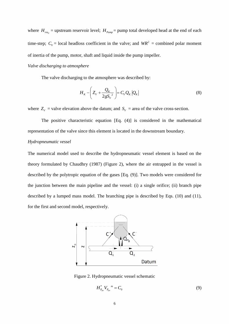
Hydropneumatic vessel

The numerical model used to describe the hydropneumatic vessel element is based on the

theory formulated by Chaudhry (1987) (Figure 2), where the air entrapped in the vessel is

described by the polytropic equation of the gases [Eq. (9)]. Two models were considered for

the junction between the main pipeline and the vessel: (i) a single orifice; (ii) branch pipe

described by a lumped mass model. The branching pipe is described by Eqs. (10) and (11),

for the first and second model, respectively.

Figure 2. Hydropneumatic vessel schematic

*

0air air

m

P PH V C (9)

7

*

air BP BPK P b P BP P PH H H Z C Q Q (10)

*

BP 22BP air

s BPBPP K P P b BP BP BP

BP BP BP

f Lg tSQ Q H H Z H C Q Q

L gD S

(11)

where *

airPH = absolute pressure head; airPV = volume of air inside the HPV at the end of the

time-step; m = exponent of the polytropic gas equation; and 0C = constant of the polytropic

gas equation given by the initial conditions *

0 0 0air air

mC H V ; bH = barometric pressure head;

PZ = water level in the HPV at the end of the time-step; BPC = local headloss coefficient of

the branch pipe; BPPQ and BPQ = flow rate through the branch pipe at the end and beginning

of the time-step, respectively; BPS = area of the branch pipe cross section; BPL = length of the

branch pipe; and BPD = inner diameter of the branch pipe.

EXPERIMENTAL FACILITY AND DATA COLLECTED

Facility description

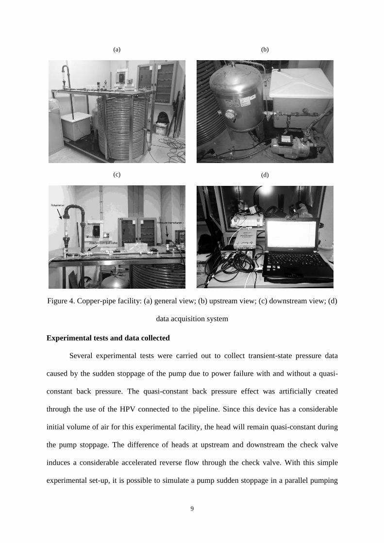
An experimental pipe rig was assembled in the Laboratory of Hydraulics and Water

Resources, in the Department of Civil Engineering, Architecture and Georessources, at

Instituto Superior Técnico (Figure 4a). The system is composed of a coiled copper pipe with

approximately 103.2 m of length, 20 mm of inner diameter and 1 mm of pipe-wall thickness.

Figure 3 presents a simplified schematic of the experimental facility.

Figure 3. Schematic of the experimental facility – adapted from Delgado (2013)

8

The system is supplied from a storage tank with 125 l of capacity by a pump with a

nominal flow rate of 1.0 m3/h, a nominal head of 32.0 m and a total power of 1.75 kW

(Figure 4b). Immediately at downstream of the pump, there is a needle check valve used to

prevent the reverse flow through the pump. At downstream the check valve, there is a

hydropneumatic vessel with 60 l of capacity (Figure 4b). This device can be connected or

disconnected from the main pipeline by the opening or close of a ball valve. At the

downstream end of the pipe, there is a ball valve with DN 3/4’’ that allow the control of the

steady-state flow rate (Figure 4c) ad the fluid is discharged in to the atmosphere at

approximately 1.51 m of elevation.

Steady-state flows are measured by a rotameter (Figure 4c) and transient-state

pressures are measured by three strain-gauge type pressure transducers (WIKA) with an

absolute pressure range from 0 to 25 bar and accuracy of 0.5% of full range. The transient-

state pressures are collected using a data acquisition system (Picoscope) with four channels

(Figure 4d). Transducers are located in different sections of the pipe: section T1 – at the

upstream end; section T2 – at a middle section; and section T3 – at the downstream end (see

Figure 3).

9

(a)

(b)

(c)

(d)

Figure 4. Copper-pipe facility: (a) general view; (b) upstream view; (c) downstream view; (d)

data acquisition system

Experimental tests and data collected

Several experimental tests were carried out to collect transient-state pressure data

caused by the sudden stoppage of the pump due to power failure with and without a quasi-

constant back pressure. The quasi-constant back pressure effect was artificially created

through the use of the HPV connected to the pipeline. Since this device has a considerable

initial volume of air for this experimental facility, the head will remain quasi-constant during

the pump stoppage. The difference of heads at upstream and downstream the check valve

induces a considerable accelerated reverse flow through the check valve. With this simple

experimental set-up, it is possible to simulate a pump sudden stoppage in a parallel pumping

10

system where only one pump trips out of two or more, where the back pressure is maintained

quasi-constant by the operating pumps.

Figure 5 presents the collected data at transducer T1, with and without the back

pressure, for initial flow rates, Q0 between 100 and 600 l/h. Figure 6 presents the

measurements at the three transducers for the transient event with Q0 = 600 l/h with and

without the backpressure.

(a)

(b)

Figure 5. Data collected at T1 for sudden pump stoppage for Q0 = 100 to 600 l/h: (a) without

back pressure; (b) with back pressure quasi-constant

(a)

(b)

Figure 6. Data collected at T1, T2 and T3 for sudden pump stoppage and Q0 = 600 l/h:

(a) without back pressure; (b) with back pressure quasi-constant

Figure 5 shows that there is a significant difference between the characteristics of the

pressure variations during the transient event, when the back pressure is affecting the flow or

11

not. When there are no back pressure, and since the geometric head between the pump and

the discharge to atmosphere is low, the fluid decelerates gradually, producing a negligible

upsurge when the check valve closes (almost not visible), and the head in the pipe system

tends to the head of the discharge to atmosphere. The oscillations observed for initial flow

rates of 100 and 200 l/h are probably due to the fact of the pump being operating far from the

rated conditions. When the back pressure is imposed on the hydraulic system, the maximum

pressures observed are extremely high. As the pump stops, the HPV holds the piezometric

head, and it starts supplying the pipeline for downstream as well as for upstream, between the

vessel and the pump; because the check valve does not instantaneously close, allowing some

reverse flow, when it actually closes, the reverse flow is quite high, inducing an extremely

high upsurge (Delgado et al., 2013). Despite not visible in Figure 5b and Figure 6b due to the

temporal scale used, the piezometric head in the experimental facility tends to the level of

discharge to atmosphere with the increase of time (due to the emptying of the HPV). This

clearly demonstrates that the back pressure have a considerable influence in the pressure

conditions during a transient event caused by the sudden stoppage of a pump.

MODEL CALIBRATION AND VALIDATION

Sudden pump stoppage without the air vessel connected

Pump-motor characteristics:

The centrifugal pump has the following rated conditions: RQ = 1.0 m3/h, pumping

head RH = 32.0 m, total power RP = 1.75 kW and rotational speed RN = 2900 rpm. The

pump-motor inertia was estimated by Thorley and Faithfull (1992) formulation, in which I =

1I + 2I , where 1I = estimated inertia of the pump impeller and fluid; and 2I = inertia of the

motor, given by

0.096

1 30.038

/1,000

R

R

PI

N

(12)

12

1.48

2 0.0043/1,000

R

R

PI

N

(13)

The pump-motor inertia was estimated in I = 0.0025 kg.m2.

Wave Speed Estimation:

The theoretical value of the wave speed was estimated in 1290 m/s by the classic

formula (Almeida and Koelle, 1992) for a copper-pipe (Young's modulus E = 177 GPa) with

20 mm of inner diameter, 1 mm of wall thickness and unconstrained throughout its length. It

was also estimated by the traveling time of the pressure wave between the downstream and

the upstream transducer, being the obtained value 1150 m/s. This value is much lower than

the theoretical value because there is gas in the liquid in a free form and cumulated in air

pockets along the pipeline. The experimental value of the wave speed (1150 m/s) is used in

all simulations.

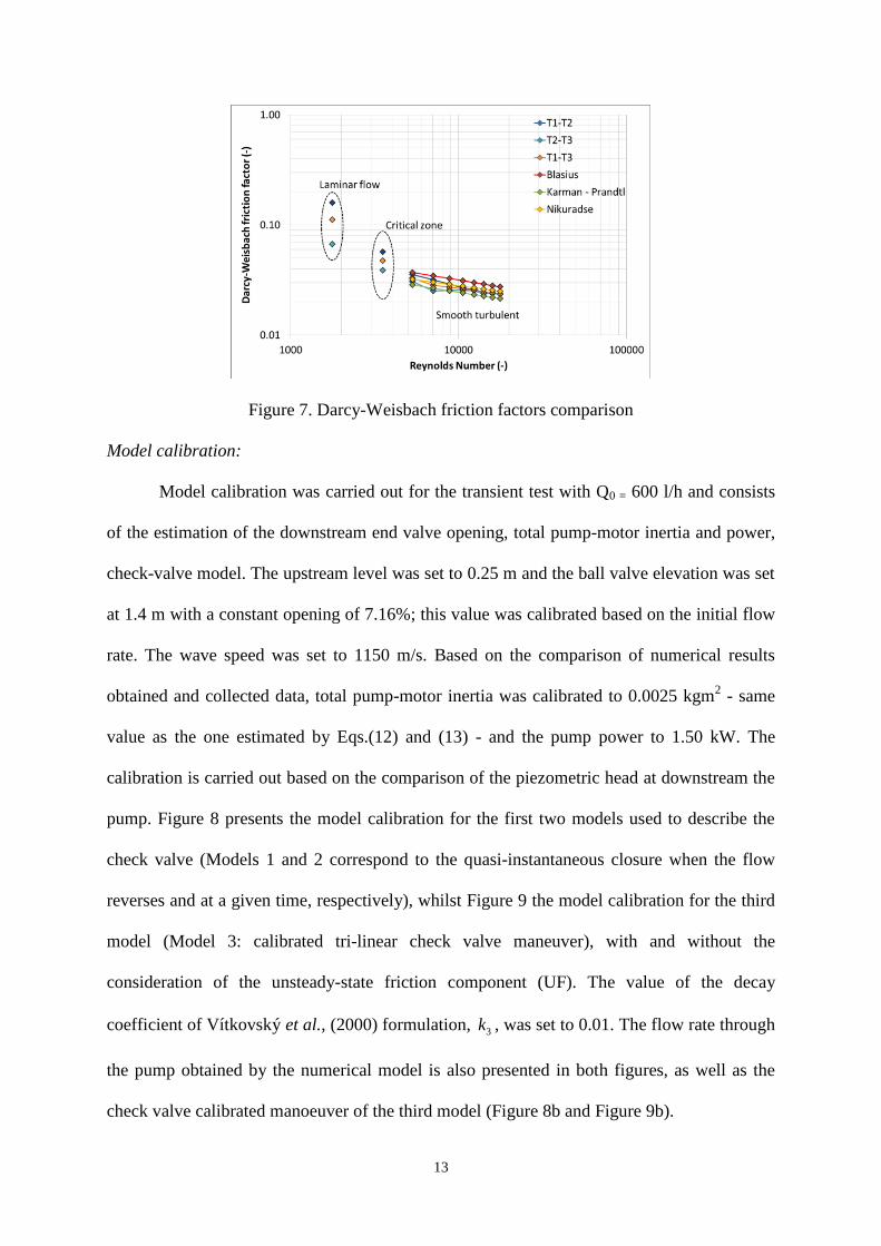
Steady-state friction resistance:

The Darcy-Weisbach friction factor was estimated based on the headlosses observed

between the three transducers and was compared with the values obtained by several friction

resistance formulas (Figure 7) presented in Eqs. (14) to (16), since the pipe-wall is smooth

(White, 1999; Lencastre, 1996). Nikuradse formulation [Eq. (15)] had a better fitting and

consequently was used to describe the steady-state friction losses in the numerical model.

Blasius Expression 0.25

0.3164

Resf (14)

Nikuradse Expression 0.237

0.2210.0032

Resf (15)

Karman-Prandtl Expression 10

1 2.512log

Res sf f

(16)

13

Figure 7. Darcy-Weisbach friction factors comparison

Model calibration:

Model calibration was carried out for the transient test with Q0 = 600 l/h and consists

of the estimation of the downstream end valve opening, total pump-motor inertia and power,

check-valve model. The upstream level was set to 0.25 m and the ball valve elevation was set

at 1.4 m with a constant opening of 7.16%; this value was calibrated based on the initial flow

rate. The wave speed was set to 1150 m/s. Based on the comparison of numerical results

obtained and collected data, total pump-motor inertia was calibrated to 0.0025 kgm2 - same

value as the one estimated by Eqs.(12) and (13) - and the pump power to 1.50 kW. The

calibration is carried out based on the comparison of the piezometric head at downstream the

pump. Figure 8 presents the model calibration for the first two models used to describe the

check valve (Models 1 and 2 correspond to the quasi-instantaneous closure when the flow

reverses and at a given time, respectively), whilst Figure 9 the model calibration for the third

model (Model 3: calibrated tri-linear check valve maneuver), with and without the

consideration of the unsteady-state friction component (UF). The value of the decay

coefficient of Vítkovský et al., (2000) formulation, 3k , was set to 0.01. The flow rate through

the pump obtained by the numerical model is also presented in both figures, as well as the

check valve calibrated manoeuver of the third model (Figure 8b and Figure 9b).

14

(a)

(b)

Figure 8. Model calibration for sudden pump stoppage without air vessel Q0 = 600 l/h –

Check valve models 1 and 2: (a) piezometric head at downstream the pump; (b) flow rate

downstream the pump

(a)

(b)

Figure 9. Model calibration for sudden pump stoppage without air vessel Q0= 600 l/h –

Check valve model 3 with and without UF: (a) piezometric head at downstream the pump; (b)

flow rate downstream the pump

Check valve Models 1 and 2 accurately describe the initial pressure drop after the

pump sudden stoppage (Figure 8a). However, the small pressure rise after the check valve

closure is not well simulated: the pressure rise occurs earlier than observed for Model 1, and

the estimated overpressures are higher than observed for Model 2. This is due to the fast

closure of the check valve, with significant reverse velocity (Figure 8b).

15

Results obtained by Model 3 used to describe the check valve maneuver fit better the

collected data. This is related with the inertial effects of accelerating and decelerating flow

through the check valve. Further experimental analyses should be carried out to identify the

relation between the accelerating and decelerating flow and the valve closure, however this is

out of the scope of the current research.

Figure 9b shows that the unsteady-state friction component has a negligible effect in

the surge damping. This is due to the fact of the transient event being slow (i.e., the flow rate

in the pump reduces to zero before the pressure wave reaches the pump element - tm > 2L/c =

0.18 s).

Model validation:

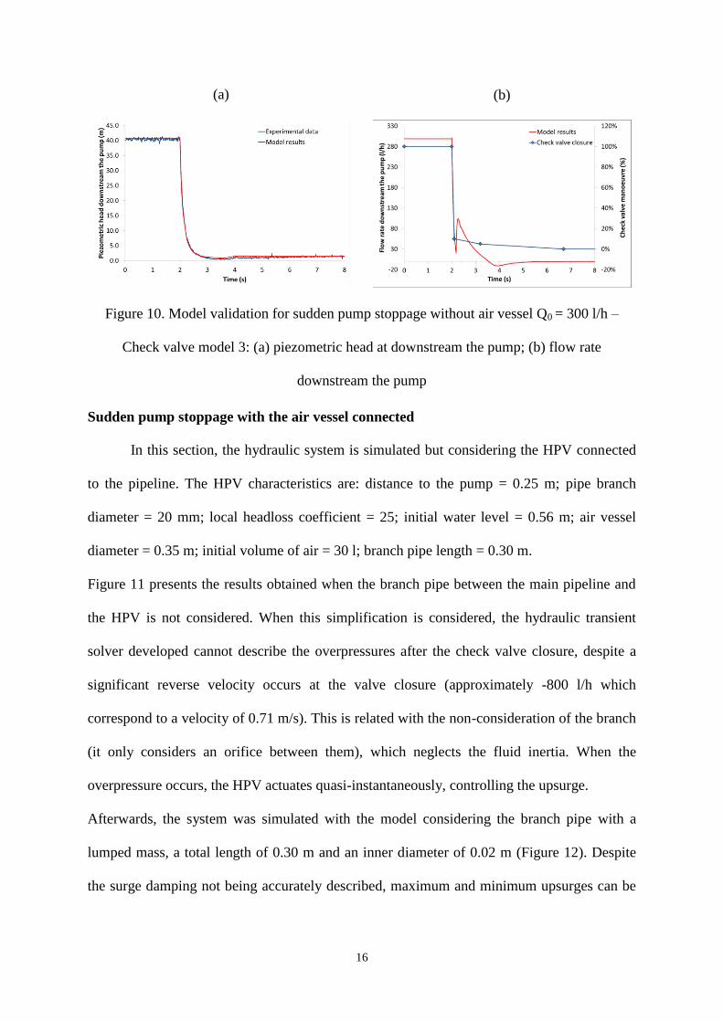
Previous values were used for model testing with different initial conditions, Q0 = 300

l/h. The power was set in 2.00 kW and the downstream end valve opening in 4.92% for this

initial condition. A good fitting is obtained (Figure 10a), as long as the check valve maneuver

is calibrated for this specific case (Figure 10b). Calibrated check valve maneuver is slightly

different from the one obtained for the Q0 = 600 l/h (Figure 9b), as the dynamic behavior of

the check-valve is different, due to change of the flow deceleration conditions. The unsteady-

state friction component was not considered in the model validation due to the negligible

influence on the surge damping description.

16

(a)

(b)

Figure 10. Model validation for sudden pump stoppage without air vessel Q0 = 300 l/h –

Check valve model 3: (a) piezometric head at downstream the pump; (b) flow rate

downstream the pump

Sudden pump stoppage with the air vessel connected

In this section, the hydraulic system is simulated but considering the HPV connected

to the pipeline. The HPV characteristics are: distance to the pump = 0.25 m; pipe branch

diameter = 20 mm; local headloss coefficient = 25; initial water level = 0.56 m; air vessel

diameter = 0.35 m; initial volume of air = 30 l; branch pipe length = 0.30 m.

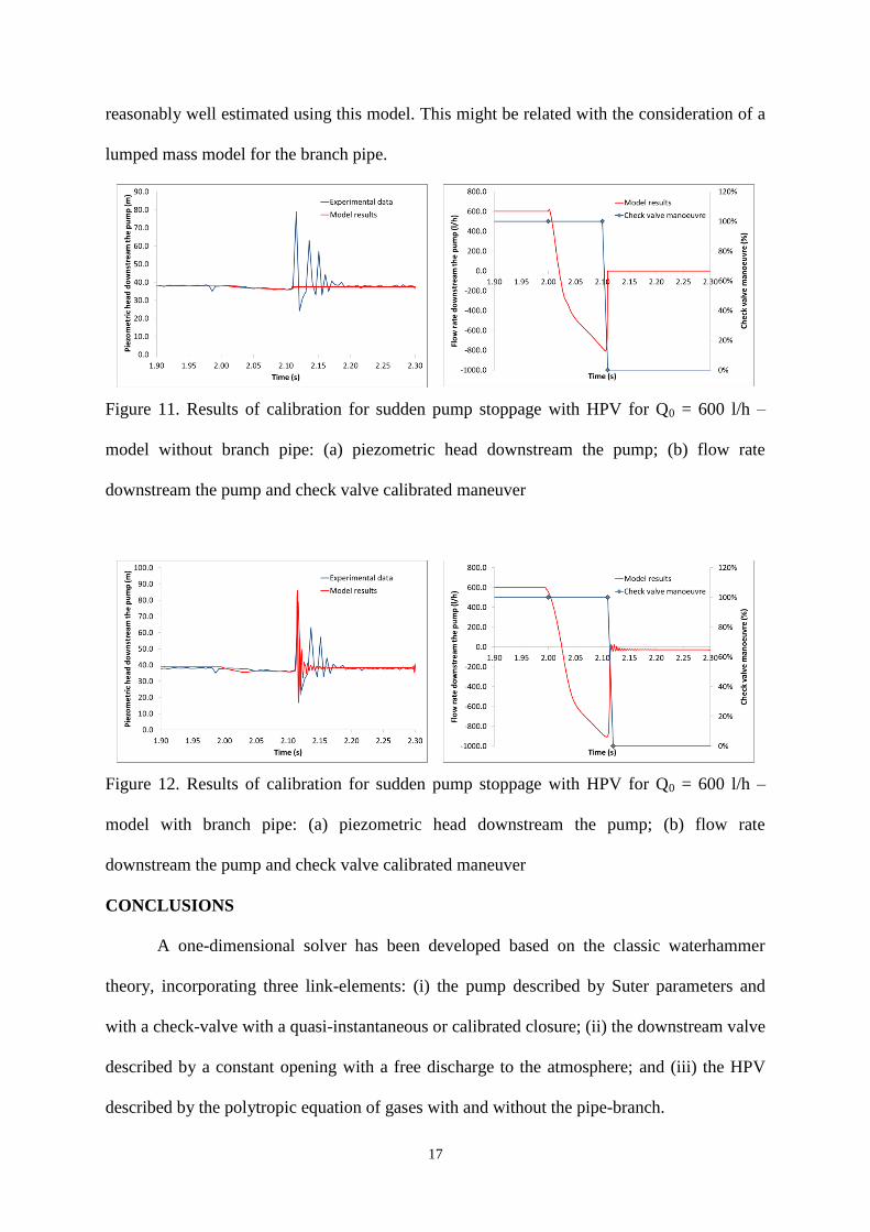
Figure 11 presents the results obtained when the branch pipe between the main pipeline and

the HPV is not considered. When this simplification is considered, the hydraulic transient

solver developed cannot describe the overpressures after the check valve closure, despite a

significant reverse velocity occurs at the valve closure (approximately -800 l/h which

correspond to a velocity of 0.71 m/s). This is related with the non-consideration of the branch

(it only considers an orifice between them), which neglects the fluid inertia. When the

overpressure occurs, the HPV actuates quasi-instantaneously, controlling the upsurge.

Afterwards, the system was simulated with the model considering the branch pipe with a

lumped mass, a total length of 0.30 m and an inner diameter of 0.02 m (Figure 12). Despite

the surge damping not being accurately described, maximum and minimum upsurges can be

17

reasonably well estimated using this model. This might be related with the consideration of a

lumped mass model for the branch pipe.

Figure 11. Results of calibration for sudden pump stoppage with HPV for Q0 = 600 l/h –

model without branch pipe: (a) piezometric head downstream the pump; (b) flow rate

downstream the pump and check valve calibrated maneuver

Figure 12. Results of calibration for sudden pump stoppage with HPV for Q0 = 600 l/h –

model with branch pipe: (a) piezometric head downstream the pump; (b) flow rate

downstream the pump and check valve calibrated maneuver

CONCLUSIONS

A one-dimensional solver has been developed based on the classic waterhammer

theory, incorporating three link-elements: (i) the pump described by Suter parameters and

with a check-valve with a quasi-instantaneous or calibrated closure; (ii) the downstream valve

described by a constant opening with a free discharge to the atmosphere; and (iii) the HPV

described by the polytropic equation of gases with and without the pipe-branch.

18

Transient tests induced by the sudden pump stoppage with and without the quasi-

constant back pressure have been carried out in an experimental facility assembled at IST

made of copper with 20 mm of inner diameter and 100 m of total length. Collected data have

shown that the pressure surges can be higher when the back pressure remains constant than

when it is not. After the failure of the power grid and consequent stoppage of the pump, the

back pressure induces a higher deceleration of the flow, inducing higher reverse velocities

through the check valve when it actually closes. The higher the velocities generated the

higher the overpressures are.

The analysis has shown that a good agreement between the numerical results and

collected data can be obtained for the transients generated by the pump sudden stoppage due

to failure of the power grid, as long as a check valve manoeuver and the total motor-pump

inertia and power are calibrated based on collected transient pressure data. Nikuradse steady-

state friction formula for smooth-wall pipes was used for steady-state friction modelling and

Vítkovský et al., (2000) unsteady friction formulation was used for transient conditions. As

the pump stoppage without the influence of the back pressure corresponds to a slow transient,

the unsteady friction effects are not relevant, being absolutely indifferent considering this

phenomenon or not.

The numerical model that neglects the branch pipe between the HPV and the main

pipeline cannot accurately predict the overpressures observed. This is due to the non-

consideration of the fluid inertia inside the branch pipe, and consequently, the vessel actuates

instantaneously, controlling the surge, as the pressure rise due to the check valve closure.

Despite the good predictions of the maximum and minimum overpressures, the numerical

model could not describe the surge damping observed, which might be related with the

consideration of a mass lumped model for the water inside the branch and not an elastic

model. As future work, the dynamic equation of check valve should be included in the model

19

to betted describe this device for design purposes when there is no data for calibration. This

paper has highlighted the need for the development of more complete and robust hydraulic

transient solvers capable of describing observed real life phenomena, and that each system

has its specificities that when neglected (e.g., check valve closure, HPV branch) can lead to

wrong surges estimation that can put at stake the safety of the pipe system

ACKNOWLEDGMENTS

Authors would like to acknowledge “Fundação para a Ciência e Tecnologia” (FCT)

for the project PTDC/ECM/112868/2009 “Friction and mechanical energy dissipation in

pressurized transient flows: conceptual and experimental analysis” for funding the current

research in terms of experimental work and grants hold.

APPENDIX I - NOTATION

The following symbols are used in this paper:

a = elastic wave speed;

BPC = local headloss coefficient of the branch pipe;

VC = local headloss coefficient of the valve;

0C = constant of the polytropic gas equation.

1C = constant that depends upon the branch pipe characteristics

D = pipe inner diameter;

BPD = inner diameter of the branch pipe.

hF , F = head and torque suter Parameters;

sf = Darcy-Weisbach friction factor;

g = gravity acceleration;

H = piezometric head;

20

bH = barometric pressure head;

*

airPH = absolute pressure head;

PumpH = pump total developed head at the end of each time-step;

RH = pump rated pumping head;

UresH = upstream reservoir level;

h = dimensionless pumping head;

fh = friction losses per unit length;

sfh = steady-state component of the friction losses;

ufh = unsteady-state component of the friction losses;

k = constant that depends upon the headlosses on the branch pipe;

3k = decay coefficient of Vítkovský et al., (2000) formulation;

BPL = length of the branch pipe;

m = exponent of the polytropic gas equation;

N = pump rotational speed;

RN = pump rated rotational speed;

SN = specific rotational speed;

n = exponent of the flow;

Q = flow rate;

iQ = initial flow rate;

BPPQ , BPQ = flow rate through the branch pipe at the end and beginning of the time-step,

respectively;

RQ = pump rated flow rate;

Re = Reynolds number;

21

S = area of the pipe cross-section;

BPS = area of the branch pipe cross section;

HPVS = area of the hydropneumatic vessel cross-section;

VS = area of the valve cross-section;

T = pump torque;

RT = pump rated torque;

t = time coordinate;

airPV , airV = volume of air inside the hydropneumatic vessel at the end and beginning of the

time-step, respectively;

v = dimensionless flow rate;

2WR = combined polar moment of inertia of the pump, motor, shaft and liquid inside the

pump impeller;

PZ , Z = water level in the hydropneumatic vessel at the end and beginning of the time-step,

respectively;

VZ = valve elevation above the datum;

x = spatial coordinate along the pipe axis;

= dimensionless rotation speed;

= dimensionless torque;

t = time-step;

= relaxation coefficient for the flow-time derivative calculation;

' = kinematic fluid viscosity;

22

APPENDIX II - REFERENCES

Almeida, A. B., and Koelle, E. (1992). Fluid transients in pipe networks, Computational

Mechanics Publications, Elsevier Applied Science, Southampton, UK.

Bergant, A., Simpson, A.R., and Tijsseling, A.S. (2006). “Water hammer with column

separation: a historical review.” J. Fluids and Struct., 22(2), 135–171.

Brunone, B., Golia, U. M., and Greco, M. (1991). “Modelling of fast transients by numerical

methods.” Proc., Int. Meeting on Hydraulic Transients and Water Column Separation,

E. Cabrera and M. Fanelli, eds., IAHR, Valencia, Spain, 273–280.

Chaudhry, M. H. (1987). Applied hydraulic transients, 2nd Ed., Litton Educational, Van

Nostrand Reinhold, New York.

Covas, D. I. C. (2003). “Inverse transient analysis for leak detection and calibration of water

pipe systems–modelling special dynamic effects.” Ph.D. thesis, Univ. of London,

London.

Covas, D.I.C., Ramos, H. M., and Almeida, A.B. (2008) “Hydraulic transients in Socorridos

pump-storage hydropower system.” Proc. 10th Int. Conf. on Pressure Surges, Pub.

BHR Group Ltd., Edinburgh, UK, 47-63.

Delgado, J. (2013). “Hydraulic transients in pumping systems – numerical modelling and

experimental analysis.” M.S. thesis, Univ. of Lisbon, Lisbon.

Delgado, J., Martins, N., Covas, D.I.C. (2013). “Uncertainties in Hydraulic Transient

Modelling in Raising Pipe Systems: Laboratory Case Studies.” Proc., 12th Int. Conf.

on Computing and Control for the Water Industry, Perugia, Italy.

Lencastre, A. (1996). Hidráulica Geral,

Marchal, M., Flesh, G., and Suter, P. (1965). "The calculation of water hammer problems by

means of the digital computer." Proc. Int. Symp. Water hammer Pumped Storage

Projects, ASME, Chicago, USA.

23

Provoost, G. (1983). “A critical analysis to determine dynamic characteristics of non-return

valves.” Proc., 4th Int. Conf. on Pressure Surges, Bath, BHRA, Cranfields, England,

275-286.

Ramos, H., Almeida, A. B., Borga, A., and Anderson, A. (2005). “Simulation of severe

hydraulic transient conditions in hydro and pump systems.” Water Resour., 26(2), 7–

16.

Ramos, H. M., Covas, D.I.C., Borga, A., and Loureiro, D. (2004). “Surge damping analysis

in pipe systems: modelling and experiments.” J. Hydraul. Res., 42(4), 413-425.

Soares, A. K., Covas, D.I.C., Ramos, H. M. (2013). “Damping analysis of hydraulic

transients in pump-rising main systems.” J. Hydraul. Eng., 139(2), 233–243.

Thorley, A. R. D. (1983). “Dynamic response of check valves.” Proc., 4th Int. Conf. on

Pressure Surges, Bath, BHRA, Cranfields, England, 231-242.

Thorley, A. R. D. (1991). Fluid transients in pipeline systems, D&L George Ltd, Hadley

Wood, England.

Thorley, A. R. D., and Faithfull, E. M. (1992). “Inertias of pumps and their driving motors.”

Proc., Int. Conf. on Unsteady Flow and Fluid Transients, R. Bettess and J. Watts, eds.,

Balkema, Rotterdam, Netherlands, 285–289.

Vardy, A. E., and Brown, J. M. (2007). “Approximation of turbulent wall shear stresses in

highly transient pipe flows.” J. Hydraul. Eng., 133(11), 1219–1228.

Vítkovský, J. P., Lambert, M. F., and Simpson, A. R. (2000). "Advances in unsteady friction

modelling in transient pipe flow." Proc. 8th Int. Conf. on Pressure Surges, Pub. BHR

Group Ltd., The Hague, The Netherlands, 471-498.

White, F. M. (1999). Fluid Mechanics. 4th Edition. Singapore, McGraw-Hill.

Wylie, E. B., and Streeter, V. L. (1993). Fluid transients in systems, Prentice Hall,

Englewood Cliffs, NJ.

24

APPENDIX III – LIST OF FIGURES

Figure 1. Pump scheme used for the numerical model .............................................................. 5

Figure 2. Hydropneumatic vessel schematic ............................................................................. 6

Figure 3. Schematic of the experimental facility – adapted from Delgado (2013) .................... 7

Figure 4. Copper-pipe facility: (a) general view; (b) upstream view; (c) downstream view; (d)

data acquisition system .............................................................................................................. 9

Figure 5. Data collected at T1 for sudden pump stoppage for Q0 = 100 to 600 l/h: (a) without

back pressure; (b) with back pressure quasi-constant .............................................................. 10

Figure 6. Data collected at T1, T2 and T3 for sudden pump stoppage and Q0 = 600 l/h:

(a) without back pressure; (b) with back pressure quasi-constant ........................................... 10

Figure 7. Darcy-Weisbach friction factors comparison ........................................................... 13

Figure 8. Model calibration for sudden pump stoppage without air vessel Q0 = 600 l/h –

Check valve models 1 and 2: (a) piezometric head at downstream the pump; (b) flow rate

downstream the pump .............................................................................................................. 14

Figure 9. Model calibration for sudden pump stoppage without air vessel Q0= 600 l/h –

Check valve model 3 with and without UF: (a) piezometric head at downstream the pump; (b)

flow rate downstream the pump ............................................................................................... 14

Figure 10. Model validation for sudden pump stoppage without air vessel Q0 = 300 l/h –

Check valve model 3: (a) piezometric head at downstream the pump; (b) flow rate

downstream the pump .............................................................................................................. 16

Figure 11. Results of calibration for sudden pump stoppage with HPV for Q0 = 600 l/h –

model without branch pipe: (a) piezometric head downstream the pump; (b) flow rate

downstream the pump and check valve calibrated maneuver .................................................. 17

25

Figure 12. Results of calibration for sudden pump stoppage with HPV for Q0 = 600 l/h –

model with branch pipe: (a) piezometric head downstream the pump; (b) flow rate

downstream the pump and check valve calibrated maneuver .................................................. 17