joint sparsity for target detection - the norbert wiener ... m. nasrabadi joint sparsity for target...
TRANSCRIPT

UNCLASSIFIED
Nasser M. NasrabadiJoint Sparsity for Target Detection
Nasser M. Nasrabadi
UNCLASSIFIED
U.S. Army Research Laboratory

Introduction
• Objective: Segmentation of HSI into multiple classes (target and background) or classifyclasses (target and background) or classify individual objects (military targets) from multiple views of the same physical target.
• Assumptions– Training data: known spectral characteristics (or
images) of different classesimages) of different classes– Test data: a sparse linear combination of all
training data– In HSI Neighboring pixels: similar materials– Mutiple views of targets are similar
• Results compared to classical SVM classifiers

Hyperspectral Imagery

Pixel-wise Sparsity Model
• Background pixels approximately lie in a low-di i l bdimensional subspace
,1 1 ,2 2 , b b
b b b b b b b bi i i i N N i a a Aa αx
• Target pixels also lie in a low-dimensional subspace
t t t t t tt tA• A test sample can be sparsely represented
b
,1 1 ,2 2 , t t
t t t ti i i i N
t ti
tN
t a a a αx A
ixby
bb b t t b t i
i i i it
A A A A Ax
i i i it
i

Ilustration: Pixel-Wise Sparse Model
0 . 1 2
0 . 1 4
0 . 0 6
0 . 0 7
0 . 0 8
0 . 0 9
0 . 1
0 . 1 1t e s t s a m p l e
0 . 0 6
0 . 0 8
0 . 1
b a c k g ro u n d d ic t io n a ry
0 5 0 1 0 0 1 5 0
0 . 0 4
0 . 0 5
0 5 0 1 0 0 1 5 00 . 0 2
0 . 0 4
t a rg e t d ic t io n a ry
Target Pixel
b
Test Spectrum ix Nonzero entries
Spectral dictionary A
bb b t t b t i
i i i iti
A A A A Ax

Sparse Recovery
• Sparse coefficient is recovered by
ˆ arg min subject to A x
• For empirical data0
arg min subject toi i i i A x
0 2ˆ arg min subject to
ˆ arg min subject toi i i i
K
A x
A x
• NP-hard problemGreedy algorithms: MP OMP SP C S MP LARS
02 0arg min subject toi i i i K A x
– Greedy algorithms: MP, OMP, SP, CoSaMP, LARS
– Convex relaxation: Iterative Thresholding, Primal-Dual Interior-Point, Gradient Projection, Proximal Gradient, Augmented Lagrange Multiplier
1ˆ arg min subject toi i i i A x

Classification Based on Residuals
• Recover sparse coefficientˆ
ˆbi
i
Recover sparse coefficient
• Compute the residuals (approximation errors
ˆi ti
Compute the residuals (approximation errors w.r.t. the two sub-dictionaries)
ˆ ˆb b t t 2 2
and ˆ ˆ b bi i i i
tb t i i
tr r x A x Ax x
• Class of test pixel is made by comparing the residuals
ix

Example: Reconstruction
0 . 6
0 . 7
0 . 8
0 . 9R e c o v e r e d s p a r s e c o e f f i c i e n t s
ˆ b
0 2
0 . 3
0 . 4
0 . 5ˆˆ
bi
i ti
0 5 0 1 0 0 1 5 0 2 0 0 2 5 00
0 . 1
0 . 2
0 . 1 2
0 . 0 8
0 . 1
ˆ ˆt t t Ax
0 . 0 2
0 . 0 4
0 . 0 6
O r i g i n a lR e c o n s t r u c t e d fr o m b g d i c .
i iAx
ˆ ˆib
ib b Ax
0 5 0 1 0 0 1 5 00
0 0
e c o s t u c t e d o b g d cR e c o n s t r u c t e d fr o m t a r g e t

Joint Sparsity Model(Joint Structural Sparsity Prior)
• Use of contextual information– Neighboring pixels: similar spectral characteristicsg g p p– Approximated by the same few training samples, weighed
differently• Consider T pixels in a small neighborhood• Consider T pixels in a small neighborhood
1 1 AA
x
2 2 Ax
1 2 1 2T T S
X x x x A AS
– ’s: sparse vectors with same support, different magnitude
T T Ax
i p pp , g– : sparse matrix with only a few nonzero rows
i
S

Illustration: T=3x3 Neighborhood
0.140.14
9
0.1
0.12
0.08
0.1
0.12
0 04
0.06
0.08
0.04
0.06 T=9
0 50 100 1500.02
0.04
0 50 100 1500
0.02
X Spectral dictionary A Row-sparse t i S
Data matrixmatrix S

Joint Sparse Recovery
• is recovered byS
• Solved by greedy algorithms: Simultaneous OMProw, 0
ˆ arg min subject to S S AS X
• Solved by greedy algorithms: Simultaneous OMP (SOMP) , Simultaneous SP (SSP) or Convex optimization to find the same active set
1,2ˆ arg min subject to S S AS X
• Decision obtained by comparing total residuals

Comparison of single pixel sparsity model VS Joint Sparsity Recovery
Model (k=5 atoms active)
Input a singleInput a single background pixel x
0ˆ arg min subject to A x
Input nine put e
neighboringbackground pixels X
row, 0ˆ arg min subject to S S AS X

Results on HYDICE FR-I
Original image (averaged Proposed detector outputg g ( gover 150 bands)
p p

Results on FR-I: ROC Curves

Extension to Multiple Classes
• AVIRIS HSI data set with 16 classes, 220 bands, 20 meters pixel resolution220 bands, 20 meters pixel resolution

Extension to Multiple Classes

Multi-View Target Classification
• In ATR applications we can have multiple observations of the same physical target from p y gdifferent platforms or from the same platform at different viewing angles (aspects).g g ( p )
0ˆ arg min subject toi i i i A y
ˆ
(Single-Measurement)
row, 0ˆ arg min subject to S S AS Y (Multi-Measurements)

Experimental Results on Multi-View Target Classification
• MSTAR SAR data-base consists of 10 militaryconsists of 10 military targets at roughly 1-3 interval azimuth angles (0-360 ) t t diff t
360 ) at two different depression angles 15 and 17 . Data from 17 is used for
training (dictionary design) 15 is used for testing

Experimental Results on Multi-View Target Classification
• Three class (BMP2, BTR70, T72) target classification C=3 with multiple views M=3 . Features are incoherent random projections dimension range from d=128 to1024.
0ˆ arg min subject toi i i i A x
1 1
0ˆ arg min subject to
and
A x
xA x
row, 0
1
ˆ arg min subject to
Note [ ]M
S S AS X
S
M M x

Experimental Results on Number of Views and Angle Size
• Effect of different number of views M
• Effect of the angle size between the views
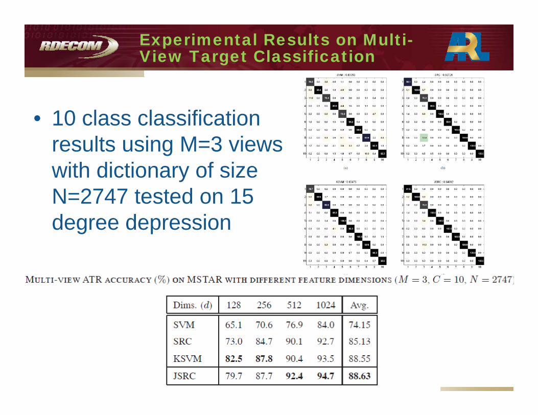
Experimental Results on Multi-View Target Classification
• 10 class classification results using M=3 views with dictionary of size yN=2747 tested on 15 degree depression g p

Multi-Pose Face Recognition
• Scenarios where we have multiple poses of the same face as input to the classifier.
• UMIST database consists of 564 images of 20 individuals with a range of poses.
• Randomly select 10 poses for each individual to construct the dictionary.

Conclusions
• Formulated target and object recognition as joint sparsity underdetermined regression problem.
• Investigated the effect single vs multiple measurements • Included the idea of joint structured sparsity prior into
th l i ti t f th ti i tithe regularization part of the optimization• Investigated performance of multiple measurements on
classification performance on several data bases. p

Thank You
THANK YOU