Joint Source-Channel Coding for Deep Space ImageTransmission using Rateless codes

Ozgun Y. Bursalioglu, Giuseppe CaireMing Hsieh Department of Electrical Engineering

University of Southern CaliforniaEmail: bursalio, caire@usc.edu

Dariush DivsalarJet Propulsion Laboratory

California Institute of TechnologyEmail: Dariush.Divsalar@jpl.nasa.gov

Abstract—A new coding scheme for image transmission overnoisy channel is proposed. Similar to standard image com-pression, the scheme includes a linear transform followed byembedded scalar quantization. Joint source-channel coding isimplemented by optimizing the rate allocation across the sourcesubbands, treated as the components of a parallel source model.The quantized transform coefficients are linearly mapped intochannel symbols, using systematic linear encoders of appropriaterate. This fixed-to-fixed length “linear index coding” approachavoids the use of an explicit entropy coding stage (e.g., arithmeticor Huffman coding), which is typically non-robust to post-decoding residual errors. Linear codes over GF (4) codes areparticularly suited for this application, since they are matchedto the alphabet of the quantization indices of the dead-zoneembedded quantizers used in the scheme, and to the QPSKmodulation used on the deep-space communication channel.Therefore, we optimize a family of systematic Raptor codes overGF (4) that are particularly suited for this application since theyallow for a continuum of coding rates, in order to adapt to thequantized source entropy rate (which may differ from imageto image) and to channel capacity. Comparisons are providedwith respect to the concatenation of state-of-the-art image codingand channel coding schemes used by Jet Propulsion Laboratories(JPL) for the Mars Exploration Rover (MER) Mission.

I. INTRODUCTION

In conventional image transmission over noisy channels, thesource compression and channel coding stages are designedand applied separately. Image coding is usually implementedby a linear transformation (transform coding), followed bythe quantization of the transform coefficients, and by entropycoding of the resulting redundant discrete source formed by thesequence of quantization indices. Due to the catastrophic be-havior of standard entropy encoding/decoding schemes, evenif only a few bits are in error after the channel decoder, thedecompressed source transform coefficients are dramaticallycorrupted, resulting in a substantially useless reconstructedimage. In order to prevent this catastrophic error propagation,the source is partitioned into blocks, such that the errors areconfined in the blocks, at the cost of some extra redundancy. Inorder to preserve integrity, which is a strict requirement in deepspace exploration scientific missions, blocks affected by errorsare requested for retransmission, at the cost of significant extra

This research in part was carried out at the Jet Propulsion Laboratory,California Institute of Technology, under a contract with NASA. The workby the University of Southern California, and JPL was funded through theNASA/JPL/DRDF/SURP Program.

delay and power expenditure. Furthermore, due to the typicallysharp waterfall BER behavior of powerful modern codes, whenchannel conditions change due to different atmospheric con-ditions, or antenna misalignment, the resulting post-decodingBER may rapidly degrade, producing a sequence of highlycorrupted images that need retransmission.

In this paper we consider a scheme for Joint Source-ChannelCoding (JSCC) that avoids conventional entropy coding. ThisJSCC scheme [1], [2] consists of a wavelet transform, a scalarembedded quantizer, and linear encoding of the quantizationindices. These three components are examined in SectionsIII, IV and V. Before getting into the details of transform,quantizer and linear code design, Section II introduces the no-tation used throughout the paper and define the relevant systemoptimization problem for JSCC based on the concatenationof embedded quantization and channel coding in general, forpractical quantization defined in terms of an operational ratedistortion function, and practical coding defined in terms of acertain overhead from capacity.

II. SYSTEM SETUP

For the problem at hand, the deep-space transmission chan-nel is represented by the discrete-time complex basebandequivalent model

yi =√

Esxi + zi, (1)

where yi ∈ C, xi is a QPSK symbol and zi ∈ CN (0, N0) isthe complex circularly symmetric AWGN sample.

Consider a “parallel” source formed by s independentcomponents. A block of source symbols of length K isdenoted by S ∈ Rs×K , where the i-th row of S, denoted byS(i) = (S

(i)1 , . . . , S

(i)K ), corresponds to a source component of

the parallel source.A (s × K)-to-N source-channel code for transmitting the

source block S onto the channel (1) is formed by an encodingfunction that maps S into a codeword of N QPSK symbols,and by an encoding function that maps the sequence of channeloutputs (y1, . . . , yN ) into the reconstructed source block S.

We consider a Weighted MSE (WMSE) distortion measuredefined as follows. Let the MSE for the ith source componentbe given by di = 1

KE[∥S(i) − S(i)∥2]. Then, the WMSE

distortion at the decoder is given by

D =1

s

s∑i=1

vidi, (2)

where vi ≥ 0 : i = 1, . . . , s, are weights that dependon the specific application. In our case, these coefficientscorrespond to the weights of a bi-orthogonal wavelet transformas explained in Section III.

Let ri(·) denote the R-D function of the ith source compo-nent with respect to the MSE distortion. Then the R-D functionof S with respect to the WMSE distortion is given by

R(D) = min1

s

s∑i=1

ri(di), subject to1

s

s∑i=1

vidi = D, (3)

where the optimization is with respect di ≥ 0 : i = 1, . . . , s,corresponding to the individual MSE distortions of the ith

source components. For example, for parallel Gaussian sourcesand equal weights (vi = 1 for all i), (3) yields the well-known“reverse waterfilling” formula (see [3, Theorem 10.3.3]).

For a family of successively refinement codes with R-Dfunctions ri(d) : i = 1, . . . , s, assumed to be convexand non-increasing [4], and identically zero for d > σ2

i∆=

1KE[∥S(i)∥2], the operational R-D function of the parallelsource S is also given by (3). Therefore, in the following,R(D) is used to denote the actual operational R-D function offor some specific, possibly suboptimal, successive refinementcode.

For a source with a total number of samples equal to Ks,encoded and transmitted over the channel using N channeluses, we define b = N/(Ks) as the number of channel-codedsymbol per pixel (spp). Hence, b is a measure of the systembandwidth efficiency. Obviously, the minimum distortion Dthat can be achieved at channel capacity C and bandwidthexpansion b is given by D = R−1(bC).

III. WAVELET TRANSFORM

The image is decomposed into a set of “parallel” sourcecomponents by a Discrete Wavelet Transform (DWT). Here,we use the same DWT of JPEG2000 [5]. With W levelsof DWT, the transformed image is partitioned into 3W + 1“subbands”. A subband decomposition example is given inFig. 1 for W = 3. This produces 3W + 1 = 10 sub-bands, which in the figure are indicated by LL0, HL1, LH1,HH1, HL2, LH2, HH2, HL3, LH3, HH3, respectively. Thesubbands have different lengths, all multiples of the LL0subband length. For simplicity, here we partition the DWTinto source components of the same length, all equal to thethe length of the LL0 subband. This yields s = 22W sourcecomponent blocks of length K = K2/s, where K × Kindicates the size of the original image. Since the DWT is abi-orthogonal transform, the MSE distortion in pixel domainis not equal to the MSE distortion in wavelet domain. In ourcase, for W = 3, the weight of a source component blockin subband w = 1, . . . , 10 is given by the w-th coefficientof the vector [l6, l5h, l5h, l4h2, l3h3, l3h3, l2h2, lh, lh, h2],

where, for the particular DWT considered in this work(namely, the CDF 9/7 [6] wavelet used by JPEG2000 for lossycompression), we have l = 1.96 and h = 2.08.

Figure 1. W = 3, partitioning of an image into 10 subbands and 64 sourcecomponents.

The subband LL0 (that coincides with the first sourcecomponent of the parallel source model) consists roughly of adecimated version of the original image. As explained in [7],in order to obtain better compression in the transform domain,Discrete Cosine Transform (DCT) is applied to subband LL0so that its energy is “packed” into a very few, very high valuedcoefficients (note the nonzero density points shown by arrowsin Fig. 2-b). These high values coefficients are separatelytransmitted as part of the header and not considered here.The remaining coefficients show sample statistics similar tothe other subbands, (see Fig. 2-c).

−1000 0 1000 20000

50

100

a−5 0 5 10

x 104

0

1

2x 10

4

b−1000 0 1000 20000

500

1000

c

−200 0 2000

500

1000

d−200 0 200

0

100

200

300

e−200 0 200

0

200

400

f

−100 0 1000

50

100

g−100 0 100

0

50

100

h−100 0 100

0

50

100

j

Figure 2. a: Histogram of 1st source component, b: Histogram of 1st sourcecomponent after DCT transform, c: Zoomed in version of b, d-j: Histogramsof source components 2− 7, respectively.

IV. QUANTIZER

The simplest form of quantization employed by JPEG2000is a special uniform scalar quantizer where the center cell’swidth is twice the width of the other cells for any resolutionlevel. This type of quantizers are called “dead-zone” quan-tizers. In Fig. 3, an embedded dead-zone quantizer is shownfor 3 different resolution levels. The number of cells at anylevel p is given by 2p+1 − 1. We indicate the cell partition at

every level by symbols 0, 1, 2 as shown in Fig.3. The scalarquantization function is denoted as Q : R → 0, 1, 2P , where2P+1−1 is the number of quantization regions for the highestlevel of refinement.

Figure 3. Quantization cell indexing for an embedded dead-zone quantizerwith p = 1, 2, 3

Let U(i) = Q(S(i)) denote the sequence of ternary quan-tization indices, formatted as a P × K array. The p-th rowof U(i), denoted by U

(i)(p,:), is referred to as the p-th “symbol-

plane”. Without loss of generality, we let U(i)(1,:), . . . ,U

(i)(P,:) de-

note the symbol-planes with decreasing order of significance.A refinement level p consists of all symbol planes from 1 top. The quantization distortion for the i-th source componentat refinement level p is denoted by DQ,i(p).

The quantizer output U(i) can be considered as a discretememoryless source, with entropy rate H(i) = 1

KH(U(i)) (inbits/source symbol). Using the chain rule of entropy [3], thiscan be decomposed as H(i) =

∑Pp=1 H

(i)p , with

H(i)p =

1

KH(U

(i)(p,:)

∣∣∣U(i)(1,:), . . . ,U

(i)(p−1,:)

), p = 1, . . . , P.

(4)Then, the set of R-D points achievable by the concatenationof embedded scalar quantizer using 0, 1, . . . , P quantizationlevels 1 and an entropy encoder is given by p∑

j=1

H(i)j , DQ,i(p)

, p = 0, . . . , P, (5)

where, by definition, DQ,i(0) = σ2i . Using time-sharing, any

point in the convex hull of the above achievable points is alsoachievable. Finally, the operational R-D curve ri(d) of thescalar quantizer is given by the lower convex envelope of theconvex hull of the points in (5). It is easy to see that ri(d) isa piecewise linear function. Therefore, the resulting functionri(d) is convex and decreasing on the domain DQ,i(P ) ≤d ≤ σ2

i . Fig. 4 shows, qualitatively, the typical shape of thefunctions ri(d).

As seen from Fig. 4, it is possible to represent ri(d) as thepointwise maximum of lines joining consecutive points in the

1Notice: 0 quantization levels indicates that the whole source componentis reconstructed at its mean value.

Figure 4. Piecewise linear operational R-D function for the i-th sourcecorresponding to a set of discrete R-D points.

set given in (5). Hence, we can write

ri(d) = maxp=1,...,P

ai,pd+ bi,p, (6)

where the coefficients ai,p and bi,p are obtained from (5)(details are trivial, and omitted for the sake of brevity). Using(6) into (3), we obtain the operational R-D function of theparallel source as the solution of a linear program. Introducingthe auxiliary variables γi, the minimum WMSE distortion withcapacity C and bandwidth expansion b is given by

Min Weighted Total Distortion (MWTD):

minimize1

s

s∑i=1

vidi

subject to1

s

s∑i=1

γi ≤ bC,

DQ,i(P ) ≤ di ≤ σ2i , ∀ i,

γi ≥ ai,pdi + bi,p, ∀ i, p. (7)

(linear program in di and γi, that can be solved bystandard optimization tools).

Note that MWTD problem (7) is derived assuming separatesource and channel coding scheme and a capacity achievingchannel code. On the other hand, for the proposed JSCCscheme, each refinement level (symbol plane) of each sourcecomponent is encoded separately with some practical code. Forexample, consider the pth plane of the ith source componentwhose conditional entropy is given by H

(i)p , let n

(i)p denote

the number of encoded channel symbols for this plane. Thesum

∑si=1

∑Pp=1 n

(i)p yields the overall coding block length

N (channel symbols). Consistent with the definition of theRaptor code overhead for channel coding applications [8], wedefine the overhead θ

(i)p for JSCC as the factor relating n

(i)p

to its ideal value KH(i)p /C as follows:

n(i)p =

KH(i)p (1 + θ

(i)p )

C. (8)

As shown in [1], the MWTD problem for JSCC with overheadsθ(i)p and entropies H

(i)p takes on the same form of (7), where

the coefficients ai,p, bi,p) correspond to the modified R-Dpoints p∑

j=1

H(i)j (1 + θ

(i)j ), DQ,i(p)

, p = 0, . . . , P, (9)

instead of (5). For given code families and block lengths, theoverhead factors θ

(i)p are experimentally determined, and used

in the system design according to the modified optimizationproblem (7). Fortunately, the overhead factors are only sensi-tive to the entropy of the plane H

(i)p , and to the coding block

length (which is an a priori decided system parameter). Henceinstead of finding θ

(i)p for each i and p, one can simply find

the overheads for different entropy values on a sufficiently finegrid.

To get an idea about the range of entropy values resultingfrom deep-space image quantization, here we report the con-ditional entropies of the first source component of an imagefrom the Mars Exploration Rover.2 We have:

H(1)1 , . . . , H

(1)8 =

0.0562, 0.0825, 0.2147, 0.4453,

0.8639, 1.1872, 1.1917, 1.1118(10)

These values span the range of entropy values for all MERimages we used in this work, and can be considered as“typical” for this application.

V. CODE DESIGN

In this section we discuss the code design for a singlediscrete source of entropy H , corresponding to a symbol plane,and the QPSK/AWGN channel with capacity C. For notationsimplicity, source and plane indices are omitted.

As discussed in Sec. I, in the proposed JSCC schemesymbol planes are directly mapped to channel symbols. Sincesymbol planes are nonbinary, i.e. 0, 1, 2, and we considerQPSK modulation, we consider linear codes over GF (4).This is particularly well suited to this problem for the fol-lowing reason. Assume that a block length of K symbolsis encoded by a systematic encoder of rate K/(K + n).Only the n parity symbols are effectively sent through thechannel. At the receiver, the decoder uses the a-priori non-uniform source probability for the systematic symbols andthe posterior symbol-by-symbol probability (given the channeloutputs y1, . . . , yn) for the parity symbols. It turns out thatif the physical channel is “matched”, such that the transitionprobability is symmetric (in the sense defined by [9]) with re-spect to the sum operation in GF (4), then the source-channeldecoding problem is completely equivalent to decoding the all-zero codeword of the same systematic code, transmitted overa “virtual” two-block symmetric channel (see Fig.5), wherethe first K symbols go through an additive noise channelover GF (4) whose noise sequence realization is exactly equalto the source block, and the remaining n parity symbols go

2Specifically image, “1F178787358EFF5927P1219L0M1”.

through the physical channel. This equivalence holds also forthe Belief Propagation iterative decoder (see [2] for details).Notice that the additive noise channel over GF (4) has capacity2−H bit/symbol, where H is the source entropy. It turns outthat if we represent the symbols of GF (4) using the additivevector-space representation of the field over GF (2), i.e., as thebinary pairs (0, 0), (0, 1), (1, 0), (1, 1) and map the “bits” overthe QPSK symbols using Gray mapping, then the symmetryof the physical channel under GF (4) sum holds. Therefore,systematic linear coding over GF (4) is particularly suited to“linear index coding” of the symbol planes produced by theembedded dead-zone quantizer and for the QPSK/AWGN deepspace communication channel.

Figure 5. Block memoryless channel with two symmetric channel compo-nents

Given this equivalence, it turns out that the optimizationof a linear systematic code ensemble for the source-channelcoding problem is obtained through the more familiar opti-mization for a channel coding problem, where the channel iscomposite, and consists of two blocks, one discrete symmetricquaternary DMC with capacity 2 − H , and one quaternary-input continuous output symmetric channel induced by (1) andby Gray mapping, with capacity 0 ≤ C ≤ 2 (that depends onthe SNR

∆= 10 log10 Es/N0).

Different symbol planes may have different entropies andtherefore they may result in codes with different overheadvalues for various SNR conditions. Nonuniversality of Raptorcodes is shown in [8] using the fact the Stability Condition onthe fraction of degree-2 output nodes depends on the channelparameter for Binary Symmetric and Binary Input AWGNchannels. Following the derivation in [8], we establisheda stability condition on degree-2 output nodes which is afunction of both H and C. Hence the code ensembles mustbe optimized for each pair of (H,C) values. In this paper,we consider the optimization of Raptor codes over GF (4)for various H and C pairs chosen with respect to a finegrid spanning the typical range of the source symbol planeentropies (see (10)) and the typical range of deep spacechannel capacities [10].

In order to optimize the Raptor code ensembles, we consideran EXIT chart and linear programming method inspired by [8]and [9], extended to handle the two-block memoryless channelas in Fig. 5.

A. EXIT CHART ANALYSIS

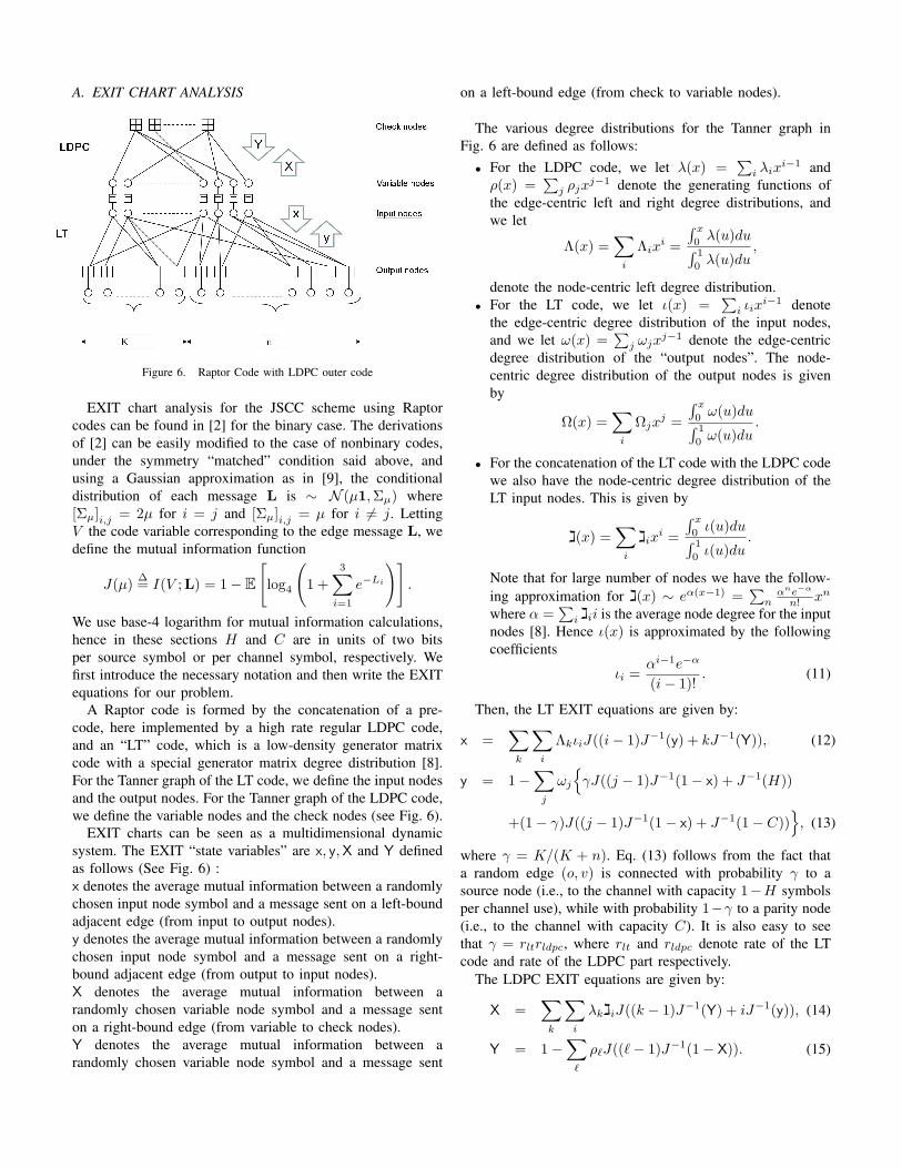
Figure 6. Raptor Code with LDPC outer code

EXIT chart analysis for the JSCC scheme using Raptorcodes can be found in [2] for the binary case. The derivationsof [2] can be easily modified to the case of nonbinary codes,under the symmetry “matched” condition said above, andusing a Gaussian approximation as in [9], the conditionaldistribution of each message L is ∼ N (µ1,Σµ) where[Σµ]i,j = 2µ for i = j and [Σµ]i,j = µ for i = j. LettingV the code variable corresponding to the edge message L, wedefine the mutual information function

J(µ)∆= I(V ;L) = 1− E

[log4

(1 +

3∑i=1

e−Li

)].

We use base-4 logarithm for mutual information calculations,hence in these sections H and C are in units of two bitsper source symbol or per channel symbol, respectively. Wefirst introduce the necessary notation and then write the EXITequations for our problem.

A Raptor code is formed by the concatenation of a pre-code, here implemented by a high rate regular LDPC code,and an “LT” code, which is a low-density generator matrixcode with a special generator matrix degree distribution [8].For the Tanner graph of the LT code, we define the input nodesand the output nodes. For the Tanner graph of the LDPC code,we define the variable nodes and the check nodes (see Fig. 6).

EXIT charts can be seen as a multidimensional dynamicsystem. The EXIT “state variables” are x, y,X and Y definedas follows (See Fig. 6) :x denotes the average mutual information between a randomlychosen input node symbol and a message sent on a left-boundadjacent edge (from input to output nodes).y denotes the average mutual information between a randomlychosen input node symbol and a message sent on a right-bound adjacent edge (from output to input nodes).X denotes the average mutual information between arandomly chosen variable node symbol and a message senton a right-bound edge (from variable to check nodes).Y denotes the average mutual information between arandomly chosen variable node symbol and a message sent

on a left-bound edge (from check to variable nodes).

The various degree distributions for the Tanner graph inFig. 6 are defined as follows:

• For the LDPC code, we let λ(x) =∑

i λixi−1 and

ρ(x) =∑

j ρjxj−1 denote the generating functions of

the edge-centric left and right degree distributions, andwe let

Λ(x) =∑i

Λixi =

∫ x

0λ(u)du∫ 1

0λ(u)du

,

denote the node-centric left degree distribution.• For the LT code, we let ι(x) =

∑i ιix

i−1 denotethe edge-centric degree distribution of the input nodes,and we let ω(x) =

∑j ωjx

j−1 denote the edge-centricdegree distribution of the “output nodes”. The node-centric degree distribution of the output nodes is givenby

Ω(x) =∑i

Ωjxj =

∫ x

0ω(u)du∫ 1

0ω(u)du

.

• For the concatenation of the LT code with the LDPC codewe also have the node-centric degree distribution of theLT input nodes. This is given by

(x)ג =∑i

ixiג =

∫ x

0ι(u)du∫ 1

0ι(u)du

.

Note that for large number of nodes we have the follow-ing approximation for (x)ג ∼ eα(x−1) =

∑n

αne−α

n! xn

where α =∑

i iiג is the average node degree for the inputnodes [8]. Hence ι(x) is approximated by the followingcoefficients

ιi =αi−1e−α

(i− 1)!. (11)

Then, the LT EXIT equations are given by:

x =∑k

∑i

ΛkιiJ((i− 1)J−1(y) + kJ−1(Y)), (12)

y = 1−∑j

ωj

γJ((j − 1)J−1(1− x) + J−1(H))

+(1− γ)J((j − 1)J−1(1− x) + J−1(1− C)), (13)

where γ = K/(K + n). Eq. (13) follows from the fact thata random edge (o, v) is connected with probability γ to asource node (i.e., to the channel with capacity 1−H symbolsper channel use), while with probability 1−γ to a parity node(i.e., to the channel with capacity C). It is also easy to seethat γ = rltrldpc, where rlt and rldpc denote rate of the LTcode and rate of the LDPC part respectively.

The LDPC EXIT equations are given by:

X =∑k

∑i

λkגiJ((k − 1)J−1(Y) + iJ−1(y)), (14)

Y = 1−∑ℓ

ρℓJ((ℓ− 1)J−1(1− X)). (15)

Eqs. (12), (13), (14), and (15) form the state equations of theglobal EXIT chart of the concatenated LT – LDPC graph withparameters H,C and γ, and the degree sequences ω, ι, ρ andλ.

Let µj denote the mean of the LLR of a source variablenode connected to a checknode of degree j, given by

µj = J−1(1− J

(jJ−1(1− x)

))+ J−1(1−H).

Then, the average symbol error rate (SER) of the sourcesymbols can be approximated by

Pe =∑j

Ωj

[1−Q3

(−√µj

2

)]. (16)

B. LT Degree Optimization

For simplicity, we fix the LDPC code to be a regular (2, 100)code (rldpc = 0.98). For this LDPC code, we find the mutualinformation threshold Y0 (using (14) and (15)) such that wheny = Y0 is the input, then the LDPC EXIT converges to Y = 1.The value of Y0 depends on the LT input degree distributionι(x), which in turns depends on α via (11). Fig. 7 shows Y0

as a function of α. On the other hand, as seen from (14) and(15), Y0 does not depend on H or C. Hence, for a fixed α,we can use the same Y0(α) threshold for all H,C pairs.

5 10 15 200.2

0.3

0.4

0.5

0.6

0.7

0.8

0.9

1

Y0

α

Figure 7. LDPC mutual information threshold vs α

Next, we use (12) and (13) to eliminate x and write yrecursively. Note that the recursion for y depends on theinput Y coming from the LDPC graph. For simplicity, wedecouple the system of equations (14-15) and (12-13) by fixingthe LDPC and the target mutual information Y0(α), and bydisregarding the feedback from LDPC to LT in the BP decoder.Therefore, we let Y = 0 in (12). The recursion functionfH,C,γ,αj (y) for a degree-j output node is given in (17) on

the top of the next page. At this point, the LT EXIT recursionconverges to the target Y0 if

y < 1−∑j

ωjfH,C,γ,αj (y), ∀y ∈ [0,Y0(α)] (18)

We sample the interval [0,Y0(α)] on a fine grid of points,and obtain a set of linear constraints ωi for fixed γ. The

objective of this optimization consists of maximizing γ (thecode rate) for a given H,C pair, where the optimization iswith respect to ωi and α. Since the LDPC code is fixed, γis just a function of rlt = 1

α∑

j ωj/j. In order to linearize the

constraints in ωi we approximate γ in (18) with its idealvalue, i.e., C/(C +H), arguing that for a good code design,γ should be close to C/(C +H).

The resulting optimization problem is given by:

minα minωj α∑j

ωj

j

s. t.∑j

ωj = 1, ωj ≥ 0,

yi < 1−∑j

ωjfH,C, C

C+H ,α

j (yi),

∀yi ∈ [0,Y0(α)]. (19)

For fixed α, the inner optimization problem in (19) is a linearprogram in terms of ωi. The outer maximization of thecoding rate rlt can be obtained through an educated searchover the value α, for each pair (H,C). With some moreeffort, it is also possible to write the stability condition for thedegree-2 output nodes, that reads Ω2 ≥ g(H,C, γ), for somecomplicated function g(·) omitted here for brevity. Differentlythan in the classical memoryless stationary channel case, inour case γ appears in the condition in a non-linear manner.Therefore, instead of including the stability condition as aconstraint in the optimization, we simply check that the resultof the optimization satisfies the stability condition (otherwise,it is discarded).

VI. RESULTS

In this section, we present in some details the deep spaceimage transmission scheme currently employed by JPL -MER (Mars Exploration Rover) Mission. This scheme, thatrepresents the benchmark for comparison to the JSCC schemepresented in this paper, is based on a separated approach in-cluding a state-of-the-art image compressor, called ICER [11],and state-of-the-art channel codes for deep space transmission.ICER is a progressive, wavelet-based image data compressorbased on the same principles of JPEG2000, including a DWT,quantization, segmentation and entropy coding of the blocksof quantization indices with arithmetic coding and an adaptiveprobability model estimator based on context models. Theseblocks have differences with respect to their counterparts inJPEG2000 to handle properties of deep-space communication(details can be found in [11]).

ICER partitions an image into segments to increase robust-ness against channel errors. A segment “loosely” correspondsto a rectangular region of the image. Each image segment iscompressed independently by ICER so that decoding error dueto data loss affecting one segment has no impact on decodingof the other segments. The encoded bits corresponding to allthe segments are concatenated and divided into fixed-lengthframes, that are individually channel encoded with a fixedchannel code rate Rc ∈ Rc, where Rc denotes a finite set

fH,C,γ,αj (y)

∆=

[γJ

((j − 1)J−1(1−

∑i

ιiJ((i− 1)J−1(y))) + J−1(H)

)+ (1− γ)J

((j − 1)J−1(1−

∑i

ιiJ((i− 1)J−1(y))) + J−1(1− C)

)](17)

of possible coding rates. The channel coding rate is chosenaccording to the channel SNR.Rc can be chosen from a set of different code rates Rc

according to channel conditions.A segment is generally divided into several frames. Data

losses occur at the frame level. A whole segment is discardedeven if a single frame corresponding to that segment is lost.When a frame loss occurs, it typically affects single segment.But it could affect two segments if the lost frame straddled theboundary between two segments. If a fixed PSNR3 value istargeted, the discarded segments must be re-transmitted. Notethat the delay and the cost of retransmission and feedback issignificant when deep space image transmission is considered.In contrast, for the proposed JSCC we do not consider anyretransmission.

0 0.5 1 1.5 2 2.5 3 3.5 410

−8

10−7

10−6

10−5

10−4

10−3

10−2

10−1

100

Eb/N

o

Fra

me

Err

or

Ra

te

Rc = 1/2

Rc = 3/4

Rc = 4/5

Rc = 7/8

Figure 8. FER vs Eb/No curves for block length 16 K

In order to compare the performance of the proposed JSCCscheme with that of the baseline scheme, we first consider anexperiment where a target PSNR is fixed. For both schemes,the bandwidth expansion factor b for fixed target PSNRdepends on the particular image and on the channel SNR,Es/N0. For a given set of test images 4, we compare thetwo schemes in terms of b versus Es/N0, for the fixed targetPSNR.

As explained above, when a frame is lost, the whole segmentis retransmitted. Frame Error Rate (FER) is assumed to be

3PSNR = 10 log102i−1D

where i = 12 since for MER mission each pixelis a 12-bit value in the original image.

4Provided by JPL-MER Mission Group.

fixed during the entire transmission process. Then the numberof transmissions necessary for a segment is a geometricrandom variable with success probability depending only onthe FER and the number of frames corresponding to thesegment’s data, denoted by F . Therefore, the expected numberof transmissions for a segment is given by,

Z = (1− FER)−F .

Although this analysis is not exact, since the number offrames spanning each segment is not constant, in general, andsome frame may straddle across two segments, nevertheless wecan find tight upper and lower bounds to the average number ofchannel uses necessary to achieve the target PSNR, for givenchannel SNR and chosen coding rate Rc (details are given in[7]).

For a given SNR value, the baseline scheme chooses acode from standard JPL codes. For a well matched SNR andrate pair, the FER is very low that expected number of re-transmission is insignificant, then b is very close to the “one-shot” transmission value, i.e. B/(2Rc) where B is the totalnumber of ICER-encoded bits for the image at the given targetPSNR.

For a given code rate, as the SNR increases beyond thematched point, b will stay fixed, since re-transmissions aregetting more and more insignificant. On the other hand, whenSNR is lower than the matched point, the FER increasessignificantly and re-transmissions become significant. In thiscase, b rapidly increases and becomes much larger than itsminimum value B/(2Rc). If SNR is very low with respect toa given channel code, then it might be more advantageous toswitch to a lower rate code.

For the example considered in this paper, the target PSNRis 49 dB and the image used is 1024 × 1024 Mars imageprovided by JPL5.

In Fig.9, we compare the b vs SNR performances of JSCCand of the baseline scheme. For JSCC, nonbinary code designis considered, but one can also use binary codes after dividingeach nonbinary symbol plane into two bitplanes. This approachis taken in [7], where binary Raptor codes and protographbased binary LDPC codes are used (See [7] for details onthese codes). Here we compare all of these cases for the sakeof completeness.

- The (∗)-curve corresponds to considering ideal capacityachieving codes for each plane in the JSCC scheme. Forthe range of PSNR values relevant to the MER mission, thepure compression rate (source coding only) for the schemeconsidered here and ICER are essentially identical (see [7]for further details on pure compression). Then, if ideal codes

5The name of the Mars image is 1F178787358EFF5927P1219L0M1.pgm

are assumed for both JSCC and the baseline scheme, thebandwidth efficiency of both schemes is the same. Hence the(∗)-curve represents the best possible performance for bothschemes, assuming ideal capacity achieving channel codes.

- Very tight upper and lower performance limits (actuallyoverlapping as seen in Fig. 9) for the baseline scheme areshown by a combination of 4 knee-shaped curves, each ofwhich corresponds to one of the codes whose FER perfor-mance is shown in Fig. (8) (see [10], [12] for details). Theseparated scheme requires several retransmissions of someblocks in the regimes of SNR for which the FER of selectedcode is significant. If for some reason (e.g., atmosphericpropagation phenomena) the channel SNR worsens, eventuallythe separated scheme must decrease the coding rate and jumpto the next available lower rate code. Hence the baselinescheme’s performance is given as the lower envelope of these4 curves. Rc value corresponding to each curve is also shownin Fig. 9.

- (×)-curve is the result of EXIT calculations for protographLDPC codes while (+)-curve is the finite length results of thesame codes.

- (−)-curve is the result of EXIT calculations for binaryRaptor codes when the LDPC code described in Sec.V-Bis used with the LT degree distribution in (20). Shokrollahireported this degree distribution in [13] to be used for erasurechannels. (−−)-curve corresponds to finite length simulationsof the same degree distribution.

Ω(x) = 0.008x+ 0.494x2 + 0.166x3 + 0073x4 + 0.083x5+

0.056x8 + 0.037x9 + 0.056x19 + 0.025x65 + 0.003x66. (20)

EXIT chart analysis result for nonbinary Raptor Codes whenthe same code (i.e. with no degree optimization) is used isgiven by (−.)-curve.

- As discussed in Sec.V, we described a method for degreeoptimization when the α parameter and LDPC code is fixed.Choosing the α parameter optimally for each H,C pair is anon-trivial task. Hence we only run the degree optimizationlinear program for each H,C pair using the α value givenby the EXIT chart analysis of classic LT sequence (i.e. (−.)-curve). For the (−.)-curve, we fixed the ω(x) distributionby (20). Then, γ depends only on the α parameter. As therequired rate, i.e. γ necessarily varies with respect to H,C, αparameter of the code changes as well. ()-curve is obtainedafter optimizing the nonbinary codes for each H,C pair usingthe α value given by the EXIT chart analysis of nonbinaryRaptor codes when (20) is used. Note the improvement withrespect to non-optimized (−.)-curve, although an outer opti-mization on α is not run.

From Fig. 9, we observe that the performance of the JSCCscheme assuming ideal codes, (∗)-curve, is better than thebaseline scheme in two different aspects. First, the requiredb value is lower for any channel condition. Second, theJSCC linear encoding together with the MWTD optimizationcan provide a “smooth” trade-off unlike the “knee” shaped

curves of the separated scheme. In Fig. 9, we observe thatinfinite length nonbinary Raptor codes are competitive withthe lower envelope of the baseline scheme. We believe thatthe infinite length results can be further improved using theouter optimization on α values.

For finite length results we first focus on Es/N0 = 3 dBpoint where finite length results are obtained with classic LTsequence and optimized LT sequences. The finite length resultsof optimized and non-optimized sequences are indicated inFig. 9 with a ⋄ and , respectively. Both the ⋄ and aresignificantly above the baseline scheme’s curve. Note that atEs/N0 = 3 dB, the channel code (Rc = 3/4) of the baselinescheme is at its matched point with the given SNR. Note thatthe baseline scheme switches to Rc = 1/2 around 2.8 dB.b value of the baseline scheme significantly increases evenpasses the ⋄ point as SNR gets lower due retransmissionskeeping a fixed PSNR value. JSCC is designed to be robustto mismatched channel conditions hence JSCC can work withthe same value of b given by the vertical height of ⋄ point.Note that keeping b fixed also avoids extra transmission delayand cost. Obviously due to mismatched channel conditions,there will be residual error in plane reconstructions. But asseen in Fig. (10-14) PSNR is gracefully degraded and theimage quality given in these reconstructions are perceptuallyacceptable depending on the application since there are noartificial “block effects” due to loss segments.

Figure 10. Original image 1F178787358EFF5927P1219L0M1.pgm

REFERENCES

[1] O. Y. Bursalioglu, M. Fresia, G. Caire, and H. V. Poor, “Lossymulticasting over binary symmetric broadcast channels,” January 2011,submitted to IEEE Trans. Signal Processing available at http://www-scf.usc.edu/ bursalio/.

[2] ——, “Lossy joint source-channel coding using raptor codes,” Int.Journal of Digital Multimedia Broadcasting, vol. 2008, Article ID124685, 18 pages.

1 2 3 4 5 6

0.6

0.8

1

1.2

1.4

1.6

SNR (dB)

b

IdealProtograph EXITProtograph FiniteBinary Raptor FiniteBinary Raptor EXITNonbinary (NB) Raptor EXITOptimized (Opt) NB Raptor EXITNB Finite simulation NB Opt. Finite simulation

Rc = 7/8

Rc = 3/4

Rc = 1/2

Rc = 4/5

Figure 9. b vs SNR trade-off for various cases

Figure 11. Image reconstruction at SNR = 3 dB, PSNR = 49 dB

[3] T. Cover and J. Thomas, Elements of Information Theory. New York:Wiley, 1991.

[4] A. Ortega and K. Ramchandran, “Rate-distortion methods for imageand video compression,” IEEE Signal Process. Mag., vol. 15, no. 6, pp.23–50, Nov 1998.

[5] D. S. Taubman and M. W. Marcellin, JPEG2000: Image CompressionFundamentals, Standards, and Practices. Norwell, MA: KluwerAcademics Publishers, 2002.

Figure 12. Image reconstruction at SNR = 2.8 dB, PSNR = 48.19 dB

[6] A. Cohen, I. Daubechies, and J. Feaeveau, “Biorthogonal bases ofcompactly supported wavelets,” Pure Appl. Math., vol. 45, pp. 485–560,1992.

[7] O. Y. Bursalioglu, G. Caire, and D. Divsalar, “Joint source-channelcoding for deep space image transmission,” submitted to JPL, TMOProgr. Rep, 2010.

[8] O. Etesami and A. Shokrollahi, “Raptor codes on binary memorylesssymmetric channels,” IEEE Trans. Inform. Theory, vol. 52, no. 5, pp.

Figure 13. Image reconstruction at SNR = 2.5 dB, PSNR = 45.63 dB

Figure 14. Image reconstruction at SNR = 2 dB, PSNR = 38.60 dB

2033–2051, May 2006.[9] A. Bennatan and D. Burshtein, “Design and analysis of nonbinary ldpc

codes for arbitrary discrete-memoryless channels,” Information Theory,IEEE Transactions on, vol. 52, no. 2, pp. 549 – 583, 2006.

[10] K. Andrews, D. Divsalar, S. Dolinar, J. Hamkins, C. Jones, andF. Pollara, “The development of turbo and ldpc codes for deep-spaceapplications,” Proceedings of the IEEE, vol. 95, no. 11, 2007.

[11] A. Kiely and M. Klimesh, “The icer progressive wavelet image com-pressor,” IPN Progress Report, vol. 42-155, pp. 1–46, 2003.

[12] Low Density Parity Check Codes for Use in Near-Earth and Deep SpaceApplications. (131.1-O-2 Orange Book): Consultative Committee forSpace Data Systems (CCSDS), 2007.

[13] A. Shokrollahi, “Raptor codes,” IEEE Trans. Inform. Theory, vol. 52,pp. 2551 – 2567, June 2006.