joint risk management management section
TRANSCRIPT
I S S U E 37 • D E C E M B E R 2016
The Optimal Timing of Risk ManagementBy Kailan ShangPage 5
Risk Management
Published by the Canadian Institute of Actuaries,Casualty Actuarial Society and Society of Actuaries
Published by
JOINT RISKMANAGEMENT
SECTION
3 Chairperson’s CornerBy Thomas Weist
4 Editor’s NoteBy Robert He and Baoyan Liu (Cheryl)
5 The Optimal Timing of Risk ManagementBy Kailan Shang
18 Risk/Return, a Chimera?By Sylvestre Frezal
21 2016 Joint Risk Management Research Update
22 ORSA Process ImplementationBy Ger Bradley, Zohair Motiwalla, Padraic O’Malley and Eamonn Phelan
23 Estimating Probability of a Cybersecurity BreachBy Meghan Anthony, Maria Ishmael, Erik Santa,Arkady Shemyakin, Gary Stanull and Natalie Vandeweghe
27 Cyber Risk is OpportunityBy Michael Solomon
31 Recent Publications in Risk Management

2 | DECEMBER 2016 RISK MANAGEMENT
Risk Management
2016 SECTION LEADERSHIP
Officers Thomas Weist, FCAS, CERA, MAAA Chairperson Frank Reynolds, FSA, FCIA, MAAA Vice Chairperson Hugo Leclerc, ASA, ACIA, CERASecretary C. Ian Genno, FSA, FCIA, CERATreasurer
Council Members Mario DiCaro, FCAS, MAAARobert He, FSA, CERARahim Hirji, FSA, FCIA, MAAAYangyan Hu, FSA, EABaoyan Liu (Cheryl), FSA, MAAALeonard Mangini, FSA, MAAAMark Mennemeyer, FSA, MAAAFei Xie, FSA, FCIA
Newsletter EditorRobert He e: [email protected] Baoyan Liu (Cheryl)e: [email protected] SOA StaffKathryn Baker, Staff Editor e: [email protected] David Schraub, Staff Partnere: [email protected] Leslie Smith, Section Specialiste: [email protected] Julissa SweeneyGraphic Designer
Published by the Joint Risk Management Section Council of Canadian Institute of
Actuaries, Casualty Actuarial Society and Society of Actuaries.
This newsletter is free to section members. Current issues are
available on the SOA website (www .soa.org).
To join the section, SOA members and non-members can locate a membership
form on the Joint Risk Management Section webpage at http://www.soa
.org/jrm
This publication is provided for informa-tional and educational purposes only.
Neither the Society of Actuaries nor the respective authors’ employers make any
endorsement, representation or guar-antee with regard to any content, and
disclaim any liability in connection with the use or misuse of any information
provided herein. This publication should not be construed as professional or
financial advice. Statements of fact and opinions expressed herein are those of
the individual authors and are not neces-sarily those of the Society of Actuaries or
the respective authors’ employers.
Copyright © 2016 Canadian Institute of Actuaries, Casualty Actuarial Society and
Society of Actuaries. All rights reserved.
Issue Number 37 • December 2016

DECEMBER 2016 RISK MANAGEMENT | 3
Chairperson’s CornerBy Thomas Weist
As of late October, I have the privilege of taking over as chairperson of the Joint Risk Management Section (JRMS). Given the talented individuals in this role before
me, the shoes to fill are enormous. Fortunately, the elected mem-bers are outstanding volunteers and excited about the projects that we have underway. In addition, four new members were elected to the council. They are eager to get started and keep up the excellent work done by the JRMS. With this motivated team, I am certain we can continue to serve our members well.
Let me start my term by thanking Mark Yu for what has been a smooth transition. Second, many thanks are owed to the SOA staff David Schraub and Leslie Smith for all the advice and support given to me as a section member and as the incoming chairperson. And lastly to the reader, we have compiled the recent survey results and will ensure our projects for the upcom-ing year are in line with your interests and priorities.
I have been interested in risk management from my early days in this profession. My career began at American Re in Princeton New Jersey. As a young student, I was encouraged by our depart-ment head to co-author a paper with a colleague. It was a Call For Papers (CFP) for a DFA seminar. How many of you remember when the models were still called DFA? Anyway, I was hooked. More than half of my time as an actuary has been in an ERM role of some fashion. Attempting to understand and quantify the entire universe of risks that can affect an insurance enterprise is extremely satisfying and challenging work. I look forward to bringing this passion to serving the members.
By the time this is published, we will have had our annual face-to-face council meeting. This gives us the opportunity to review our objectives for the year and align those tasks with the members and friends of the section best suited. One of those tasks for 2016 was to promote the JRMS through networking events. This was one area where I contributed by hosting a reception at the Southwest Actuarial Forum (SWAF) at their June meeting in Dallas. We hope to do something similar at their next meeting in December in San Antonio. Additional net-working events have been held or planned in New England and Toronto as well. Our plan for 2017 is to expand on this effort.
ADDITIONAL 2016 ACHIEVEMENTS TO DATEMeeting Sessions—Section members work with meeting com-mittees on risk management sessions by moderating, presenting
or finding presenters. The JRMS participated in the following meetings: ERM Symposium, Life and Annuity Symposium, Valuation Actuary Symposium, 2016 SOA Annual Meeting & Exhibit, SOA Health meeting, and the CAS Spring & Annual meetings.
Webcasts—An Actuary’s Toolbox and Professionalism were both completed this year. Next up, we have a webcast on Economic Scenario Generators.
JRMS Newsletter—We publish three issues of Risk Managementeach year. You have all received the April and August issues and this is the final issue for 2016.
JRMS Research—The 2016 ERM Symposium CFP and a Cyber Risk CFP have been completed. The following projects are currently underway: Country Risk Officer, ERM Stakeholder Buy-in, 2016 Emerging Risk Survey, Application of Enterprise Risk Management on National Long Term Care Needs and Parameter Uncertainty. Details of these projects can be found in the Research Update later in the newsletter. We also supported the CIA in developing its ORSA Survey.
All of these important projects could not be completed without our members and the council. If you would like to participate please let us know. There are opportunities such as writing an article for the newsletter, presenting at a seminar or assisting in a research project. We are always glad to have additional vol-unteers help us with our mission to further the education and research in the area of risk management. n
Thomas Weist, FCAS, CERA, MAAA, is chief actuary at Tokio Marine HCC. He can be reached at [email protected].

4 | DECEMBER 2016 RISK MANAGEMENT
Editor’s NoteBy Robert He and Baoyan Liu (Cheryl)
In “The Optimal Timing of Risk Management,” Kailan Shang discusses methods of determining the appropriate timing of implementing a risk management strategy or investing in risk
management projects. Like investment timing, it is important to consider the timing in risk management decisions to maximize the gain of risk management projects. This topic is a very broad and important topic; the editors appreciate the author bringing this key topic to the actuarial community.
Sylvestre Frezal gives new thoughts to several common prac-tices in the industry and suggests new ways to handle challenges in “Risk/Return, a Chimera?”
We have a short update on ORSA processes and two articles on cyber risks.
“Estimating Probability of a Cybersecurity Breach” is based on research from Professor Shemyakin and his team from Uni-versity of St. Thomas. This article discusses how to estimate probability of a cybersecurity breach for a specific database application.
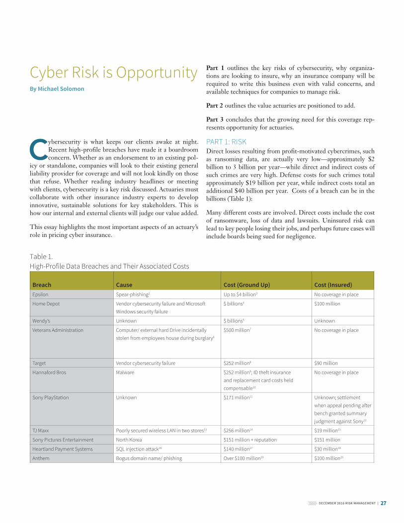
“Cyber Risk is Opportunity” is an award winning essay by Michael Solomon. The paper outlines the key risks of cyberse-curity and the value actuaries are positioned to add. The essay concludes that the growing need for this coverage represents opportunity for actuaries.
As usual, we would like to give a special thank you to David Schraub, Cheryl Liu and Kathryn Baker for helping us pull together this issue of the newsletter. n
Robert He, FSA, CERA, is VP ALM & Capital Markets at Guggenheim Insurance. He can be reached at robert.he@guggenheiminsurance .com.
Baoyan Liu (Cheryl), FSA, MAAA, is senior manager,financial risk management at FWD Life InsuranceCompany (Bermuda) Limited in Hong Kong. Shecan be reached at [email protected].

DECEMBER 2016 RISK MANAGEMENT | 5
The Optimal Timing of Risk ManagementBy Kailan Shang
Editor’s Note: This paper was originally published in the 2016 ERM Monograph. It has been excerpted here. The full paper can be found on SOA.org.
This paper explores the methods of determining the opti-mal timing for risk management projects. It discusses the timing considerations for financial risk hedging, insurance
risk hedging and investment in new risk management functions.
1. TIMING DECISION BIASESBefore discussing the approaches of formal timing deci-sion-making, it is necessary to understand the major human biases affecting timing decisions. Being aware of these biases can help us recognize our biases and improve our understanding, opinions and future decisions accordingly.
1. Herding. Herding occurs when people follow the behaviors of the majority. When a decision is made because of herding, it is dangerous because the general opinion may not be suit-able for a specific case. Without sufficient information and analysis, the decision could be made too early and too rashly and the appropriate timing is not fully considered.
2. Analysis paralysis. An over-analysis may unnecessarily defer a decision. The timing can be considered too complicated and too much information may be required before a decision can be made.
3. Shortsighted shortcuts. Russo and Schoemaker (1990) considered shortsighted shortcuts a decision trap. Deci-sion-makers may rely heavily on convenient facts, easily obtained information and rules of thumb. Like herding, shortsighted shortcuts may lead to rash decisions without full consideration of appropriate timing.
4. Shooting from the hip. Shooting from the hip means mak-ing a quick decision without a comprehensive and systematic consideration of other alternatives. As Russo and Schoemaker (1990) described, all the information is kept in the deci-sion-maker’s head and then the decision is made. Detailed analysis of optimal timing is likely to be neglected in this decision-making style.
To reduce the negative impact of human biases on timing deci-sion, a consistent decision-making approach is important. With a comprehensive analysis of the cost, benefits and potential value of new information, decision-makers can get a holistic view rather than judge based on limited information and experience.
2. NET PRESENT VALUE VERSUS REAL OPTIONWhen evaluating investment projects and making investment timing decisions, two approaches are normally used: net present value (NPV) approach and real option approach. They may also be used for optimal timing decisions.
The NPV approach measures the value of a project as the present value of future net cash flows (NCF) deducted from the initial investment costs.
Where:
NCFt: Net cash flow at time t; it is calculated as the difference between benefits and costsk: Hurdle rate; it is the expected return required from an invest-ment projectn: Time horizonC0: Initial investment at time 0NPV is the expected value of the investment. An example of using the NPV approach for timing decision is shown in Section 2.1.
2.1. Example: Investment Timing Decision Using the NPV Approach
Option 1. Start project immediately with two-year time horizon.
The initial investment is $2,000. For the first period, the NCF is $1,200. For the second period, there is a 60 percent probability that the NCF is $1,800 and a 40 percent probability the NCF is $600.

6 DECEMBER 2016 RISK MANAGEMENT
The Optimal Timing . . .
Option 2. Start project one year later with one-year time horizon.
If the company waits one year, the investment at time 1 is $1,100. The NCF of the second time period is still uncertain, as in Option 1.
With a discount rate of 10 percent, the NPV at time 0 is $165 for the first option and $83 for the second option. By choosing the greater of the two, the investment should start immediately.
However, the NPV approach does not reflect the impact of risk. It also assumes there will be no additional information in the future that can affect the decision and the NPV of future investment.
On the other hand, the real option approach incorporates the value of future information in the decision-making process. Continuing with the NPV example and assuming that the NCF at time 2 will be known exactly at time 1, a better decision could be made given the new information. If the NCF of the second period is known to be $1,800 at time 1, the investment will be made. If the NCF is known to be $600, no investment will be made.
2.2. Example: Investment Timing Decision Using the Real Option Approach
Option 1. Start project immediately with two-year time horizon.
Option 2. Start project one year later with one-year time horizon.
For both options, the NCF at time 2 is uncertain at time 0, but certain at time 1. If the investment decision is deferred to time 1, the investment will be made only if the NCF at time 2 is $1,800.
With a discount rate of 10 percent, the NPV at time 0 is $165 for the first option. Unlike the NPV approach, the NPV of the second option is calculated as By choosing the greater of the two, the investment decision should be deferred to time 1.
Therefore, when future information has immaterial impact on future decision-making, the NPV approach can be used. Otherwise, the real option approach should be adopted.
3. TIMING OF RISK MANAGEMENT DECISION-MAKINGGiven that the real option approach incorporates the value of new information in the analysis, it is more appropriate than the NPV approach for determining the appropriate timing of a risk management project. However, some adjustments are needed to reflect the differences between risk management projects and investment projects.
• The main purpose of risk management projects is to reduce risk rather than maximize investment gains. NCF in the traditional NPV calculation is the expected value and cannot reflect the benefit of loss reduction because of a risk man-agement project. Measures based on expected values are not appropriate for assessing risk management projects. Instead, NCF at a more extreme confidence level can be used. The chosen confidence level should be consistent with the com-pany’s risk appetite.
• The costs and benefits of risk management projects are com-plicated and may be different from investment projects. Some types of cost and benefit follow.
Costs:
- Project investment. This is similar to the cost in normal investment projects.

DECEMBER 2016 RISK MANAGEMENT | 7
- Hedging cost. This may include the cost of buying hedg-ing instruments such as equity index options.
- Transaction cost. Some risk management projects require dynamic trading such as in a dynamic hedging program. The transaction cost measured by bid-ask spread could be a significant part of the total cost.
- Counterparty risk. A risk management project may involve transferring risk to a counterparty. At the same time, the exposure to the counterparty risk increases.
- Loss of upside gains. A risk management project can reduce the risk but at the same time limit the upside poten-tial. The loss of gains needs to be considered in project assessment.
Benefits:
- Loss reduction. At a given confidence level or in an extreme event, a risk management project such as an interest rate risk hedging program can reduce the amount of loss.
- Potential benefit of a lower borrowing cost because of a higher credit rating. A risk management project may increase the rating on enterprise risk management, which is a key component of credit risk assessment by rating agencies. The benefit can be quantified as the product of three factors: the probability of getting a higher credit rating, the contribution of the project and the magnitude of borrowing cost reduction.
- Potential benefit of lower cost of capital. If a risk man-agement project can improve the capital adequacy and liquidity position of a company, the cost of raising addi-tional capital in a normal economic environment will be lower. The benefit is the expected reduction in the financ-ing cost.
- Potential benefit of better decisions. For example, an investment in building a more advanced risk assessment platform such as an economic capital framework could help senior management make informed decisions. The benefit of the investment is the product of the decreased probability of making a wrong decision and the cost of a wrong decision.
Most of the cost and benefit items listed require complex pre-dicting using either historical experience or experts’ opinions.
• The value of future information is necessary but difficult to quantify. To determine the optimal timing, the key is to evalu-ate how future information may improve future decisions. For example, to hedge the equity risk in a future financial crisis, equity index put options can be bought either immediately or
later. Assuming that the economy is in the expansion phase, the key value of future information is a better understanding of the time the economy will go into a recession period. If future economic data indicate a prolonged economic expan-sion phase, it may be better to defer equity risk hedging.
• Some risk management projects are divisible across time. For example, a hedging program can be implemented at several stages gradually till it is fully completed. Staged risk man-agement decisions include not only the timing but also the amount of investment at each stage. The decision-making process is even more complicated and may require dynamic programming.
With these adjustments, different timing options can be com-pared based on the NPV after considering the value of future information. In sections 4 to 6, specific considerations are discussed regarding these adjustments for different decision problems.
4. TIMING OF HEDGING FINANCIAL RISKSFor companies with significant free capital, adopting the con-trarian approach in financial risk hedging may be a good idea. If the economy has stayed in the expansion cycle for a long period and the market has started worrying about market bubbles, it is a good time to mitigate the risk being taken before the hedging cost rises. If the economy stagnates for a continued period and financial stimulus plans start to have some beneficial outcomes, it may not be a good time to reduce the risk exposure due to the high cost. On the other hand, taking risk is more profitable as most market participants are looking for counterparties to transfer the risk.
For companies in a distressed situation that still have a pretty big chance of recovery, it may be better to only hedge short-term earnings volatility to ease the panic of investors. Long-term arrangement of risk transfer in difficult times may not be a wise decision. However, these companies may not have a choice due to pressure from regulators, rating agencies, customers and the public.
A key consideration in determining the appropriate timing of hedging financial risks is the future changes in economic con-ditions. In a situation where the future economic situation is unclear, deferring the decision on financial risk hedging may buy decision-makers some time to get a better view of economic development and then make a more informed decision. In the following example, the company wants to hedge its exposure to equity risk but is also considering different timing options.
4.1. Example: Equity Risk HedgingInsurance company ABC sells variable annuity products with a guaranteed minimum account value equal to 100 percent of paid premium. It has a large exposure to equity downside risk. The

8 DECEMBER 2016 RISK MANAGEMENT
The Optimal Timing . . .
existing exposure is below the company’s risk tolerance. How-ever, the company has a business expansion plan that needs extra capital. By hedging the equity risk, some capital can be freed to support the expansion plan.
The economy has been recovering from the 2008 financial crisis for six years. It is difficult to predict whether the economy will continue expanding or move slowly into another recession. To evaluate the timing options of hedging, the company needs to predict the change in market volatility, which has a significant impact on the cost of hedging. The company plans to buy stock index put options so it can hedge the minimum guarantee but not give up the potential upside. The higher the market volatil-ity, the higher the cost of buying put options. Figure 1 shows the Standard & Poor’s 500 daily index and its volatility index from Jan. 2, 1990, to Nov. 11, 2015. Spikes of the VIX1 are normally accompanied with material downward market movements. The correlation coefficient between the daily change in the index value and the daily change in the VIX is −71 percent over the study period.
For the timing decision, an important question to answer is that given the current level of VIX, what will the value of VIX be in one month, three months and so on. If the VIX is likely to go down, the company may want to defer the hedging for a lower
cost of put options. If the VIX is likely to go up, the company may want to buy the put options immediately.
For simplicity, the only cost of the hedging program to be considered is the cost of put options. For the same reason, the price of put options is assumed to change only with the volatility parameter across time. In practice, when considering timing options, other assumptions such as interest rate can also be pre-dicted to be time variant.
The benefits of the hedging program include
• the loss reduction if the stock index value falls below the exercise price and
• the saving of the cost of raising capital for the business expan-sion plan.
Both benefits vary with the future economic environment. In an economic expansion, the benefit of loss reduction is small but the saving of capital cost is large. In an economic recession, the benefit of loss reduction is large but the saving of capital cost is zero because the company is unlikely to have enough financial resources for the expansion.
Generally speaking, the current level of market volatility has a big impact on the timing decision.
Data from Yahoo! Finance
Figure 1. S&P 500 Index Value and VIX (January 1990 to November 2015)

DECEMBER 2016 RISK MANAGEMENT | 9
• In a low volatility situation (low VIX), the cost of hedging is relatively low. It is likely the hedging program should be implemented immediately.
• In a high volatility situation (high VIX), the cost of hedg-ing is high and the loss due to the bear market has already happened. Also, the business expansion plan may need to be deferred due to stressed financial conditions. Therefore, it is likely the hedging program should be deferred.
• In a medium volatility situation (medium VIX), the timing decision becomes complicated. If the economy is heading into recession, the cost of hedging is lower now than later. The benefit of hedging is likely to be realized in the near future. In this case, it is better to implement the hedging strategy immediately. If the economy continues expanding, the cost of hedging is higher now than later and the benefit of hedging may not be realized in the near future. Because it is difficult to predict future economic conditions, it may be
worth waiting for a certain period to get a clearer idea of the direction of the economy.
Table 1 lists the transition matrix of S&P 500 VIX with a period of three months based on the data from Jan. 2, 1990, to Nov. 11, 2015. In the low volatility range (VIX <20 percent), the VIX has a very high probability of staying in the low range. In the high volatility range (VIX >30 percent), there is a high probability the VIX will go down in the next three months. In the middle volatility range (VIX ϵ [20 percent, 30 percent]), VIX has a high chance to stay in the middle range or go down. But the chance of going up is not negligible.
Assuming that the current VIX is 25 percent, which is the aver-age value in the middle range based on the experience data, the company is considering whether to implement the hedging pro-gram immediately or three months later. The company wants to hedge an equity risk exposure of $50 million for one year.
Table 1. Three-Month Transition Matrix of VIX (January 1990 to November 2015)
VIX <10% [10%, 20%) [20%, 30%) [30%, 40%) [40%, 50%) ≥50%
<10% 0.0% 100.0% 0.0% 0.0% 0.0% 0.0%
[10%, 20%) 0.3% 84.0% 12.6% 2.6% 0.5% 0.1%
[20%, 30%) 0.0% 29.5% 57.6% 9.7% 1.1% 2.1%
[30%, 40%) 0.0% 10.7% 68.5% 16.6% 3.4% 0.7%
[40%, 50%) 0.0% 0.0% 47.3% 39.3% 13.4% 0.0%
≥50% 0.0% 0.0% 1.8% 16.1% 71.4% 10.7%

10 DECEMBER 2016 RISK MANAGEMENT
The Optimal Timing . . .
Option 1. Hedge immediately.
The cost of hedging is estimated to be $3.8 million with an interest rate of 4.5 percent, an implied volatility of 25 percent2
and a term of one year using the Black-Scholes formula for a European put option.
Based on the experience data, three real world scenarios are assumed at the end of one year:
option payment ($9M × 0.18 = $1.6M) and the reduced cost of capital ($1.3M). The return on investment (ROI)3 is −23 percent and the NPV with a hurdle rate of 10 percent is −$1.1 million. From the perspective of maximizing the investment gain, Option 1 is not a good option because of negative ROI and NPV. In practice, other benefits of the hedging may exist that could improve the NPV and ROI significantly. For exam-ple, a reduction in required capital could lead to an improved capital position and a credit rating upgrade, which can reduce the borrowing cost. For simplicity, these potential benefits are not included in the example. The focus here is the comparison of the NPVs between different timing options.
Option 2. Defer hedging decision for three months.
The company also wants to consider delaying the hedging decision for three months. It has the following assumption of changes in the VIX in three months based on experience data.
Notes:
1. Three scenarios are assumed for the equity value at the end of one year. In the up scenario, the equity value is $57.2 million with a probability of 33 percent. In the middle sce-nario, the equity value is $50.8 million with a probability of 49 percent. In the down scenario, the equity value is $41 million with a probability of 18 percent. The scenarios rep-resent the average equity values for the low, medium and high VIX scenarios, respectively. Both the equity values and the probabilities are derived from the historical data of S&P 500 index and VIX from January 1990 to November 2015.
2. Only in the down scenario will the at-the-money equity put option be exercised. The payment is $9 million ($50 million – $41 million).
3. The hedging will release the required capital used to sup-port equity risk. It is assumed the company sets the required capital at a confidence level of 99.5 percent. Assuming the equity value follows a lognormal distribution with µ = 7 percent and σ = 25 percent, the required capital is calcu-lated as the cost of capital rate × initial exposure × (1 − 0.5th percentile of lognormal (µ, σ)). The cost of capital rate is assumed to be 6 percent. Initial exposure is $50 million. The 0.5th percentile of lognormal (0.07, 0.25) is the left-tail 0.5 percent value at risk (VaR). (1 − 0.5th percentile) is the smallest loss in the worst 0.5 percent scenarios and is used to calculate the required capital to be freed. The reduced cost of capital is estimated to be $1.3 million.
The cost of Option 1 is $3.8 million at time 0. The benefit is $2.9 million at the end of one year, which is the sum of the put
Notes:
1. The VIX may drop to 18 percent with a probability of 29 percent, change to 24 percent with a probability of 58 percent, and go up to 39 percent with a probability of 13 percent. Both the VIX and probability are derived from the historical data of VIX from January 1990 to November 2015.
2. The cost of buying put options at the end of three months for each scenario is calculated with an interest rate of 4.5 percent and a term of nine months. The exercise price is equal to the minimum of the equity index price at time 0 and the equity index price at the end of three months. In the low VIX scenario (up scenario for equity price), the equity value is expected to be $53.3 million. The put option to be bought at the end of three months will have an exercise value of $50 million. In the medium VIX scenario (medium scenario for equity price), the equity value is expected to be $50.9 million and the exercise value of the put option will be $50 million. In the high VIX scenario (down scenario for equity price), the equity value is expected to be $44 million. The exercise value of the put option will be $44 million

DECEMBER 2016 RISK MANAGEMENT | 11
instead of $50 million. The cost of the in-the-money put option with an exercise value of $50 million is too high in the high VIX scenario.
The following scenarios of equity values at the end of one year, given the value at the end of three months are assumed.
by the equity value dropping below $50 million. It is calculated as shown.
Using the same method as in Option 1, the benefit of hedging in each scenario (up, middle or down) at the end of three months can be calculated. The results are listed in Table 2.
Table 2. NPV Result by Scenario
Scenario Up Middle Down
NPV@10% 0.45 0.04 −5.20
ROI 70% 12% −96%
Probability 29% 58% 13%
Time Cash Flows
0 0 0 0
0.25 −1.20 −2.90 −5.80
1 1.78 3.16 0.51
Decision Hedge Hedge No
Both the up scenario and middle scenario have a positive NPV. In these scenarios, hedging is likely to be implemented at the end of three months. In the down scenario, negative NPV indi-cates the hedging strategy will not be implemented. The cost of the unhedged position in the down scenario is the loss caused
Cost of unhedged position in the down scenario = ($50M − $46.8M) × 0.65 + ($50M − $38.8M) × 0.1 = $3.2M.
The NPV of Option 2 at time 0 is −$0.2 million, calculated as the weighted average of the values in three scenarios based on the chosen strategy. The weight is the probability of each sce-nario. The value is the NPV of the hedging strategy for the up and middle scenarios and the cost of the unhedged position in the down scenario. It is much higher than the NPV of Option 1, which is −$1.1 million. Therefore, the company is better waiting three months before making decisions on hedging implementation.
In this example, a transition matrix based on experience data is used as one of many possible approaches. History may not be a good indicator of the future because of the persisting low interest rate environment, which has never happened before. Advanced predictive models adapted for the new economic regime can be used in practice. The trinomial tree can also be replaced by a stochastic model that considers thousands of scenarios.
In practice, threshold-based decision mechanism can be designed for easy monitoring. For example, the middle scenario has a near-zero NPV. A possible simplified decision-making mechanism could be that if the VIX is no greater than 24 per-cent, which is the volatility in the middle scenario, the hedging strategy will be implemented immediately. Otherwise, the deci-sion will be deferred.
4.2. Other Applications The approach used in the example in Section 4.1 can be used for other projects such as deciding the optimal timing of raising capital. The cost of financing changes with the economic envi-ronment as well. Raising additional capital during an economic

12 | DECEMBER 2016 RISK MANAGEMENT
The Optimal Timing . . .
expansion is less costly than during an economic recession. Incorporating economic cycles in the analysis can provide valuable information for decision-making regarding capital management.
5. TIMING OF HEDGING INSURANCE RISKSSimilar to the timing decision on hedging financial risks, the optimal timing of hedging insurance risks needs to consider the possible changes in costs and benefits in the future caused by changes in the market condition. In addition to the economic cycle, the insurance cycle is an important consideration for hedging insurance risks.
The insurance cycle, aka the underwriting cycle, is the cyclical pattern of insurance prices and profits for the property and casualty insurance industry. A full cycle consists of two phases: soft market and hard market. A soft market is featured with increasing competition, relaxing underwriting rules, lower insurance price and profit. With a capacity constraint or a major catastrophic event, the market moves into a hard market. A hard market is featured with stringent underwriting, higher insurance price and improved profit. Meier and Outreville (2003) showed that the return on equity (ROE) of the U.S. P&C insurance industry has a material impact on the reinsurance price. A lower ROE indicates a higher reinsurance price. A higher reinsurance price could also indicate a higher level of hedging cost for insur-ance risk.
If the hedging is not immediately needed, the company can decide the most appropriate time to implement the hedg-ing. The cost of hedging is a major component in the timing
decision. For example, a company wants to hedge its exposure to catastrophe risk by issuing catastrophe bonds. The market changed into a hard market one year ago. The company’s capital position is strong and it does not need to reduce its risk expo-sure immediately. In this case, the company may consider the following factors for its timing decision.
• When will the market move to a soft market? In a soft mar-ket, the cost of issuing catastrophe bonds will be lower. It might be worth waiting if the hedging is a long-term plan. Some models are available to predict insurance cycles such as the regime-switching model proposed by Wang et al. (2011).
• The company could also take a staged approach by issuing a small portion of the total amount in a hard market and grad-ually increasing the amount of hedging as the market moves into a soft market.
• When evaluating different timing options, the company needs to consider the potential loss caused by catastrophes during the period before hedging is in place.
The real option approach can be used in a similar way to the analysis of financial risk hedging. The value of new information is estimated using the insurance cycle modeling rather than the economic cycle modeling.
6. TIMING OF RISK MANAGEMENT INVESTMENTBuilding new risk management functions is important but also expensive. Other important projects may compete for limited resources. Unless the risk management investment is required immediately by regulators, it is helpful to study its optimal tim-ing from an economic perspective.
The benefit of building new risk management functions are difficult to quantify. For example, building an economic capital (EC) framework can improve a company’s risk analysis capability, improve future risk decisions and, in the long term, may contrib-ute to a credit rating upgrade. Unlike the examples of hedging programs in the previous sections, most of the assessments could be quite subjective and few company-specific experience can be relied on. The timing consideration is even more ambiguous. In practice, the timing is determined after the board or senior man-agement have made the decision to build the EC framework. The actual timing depends heavily on the availability of resources. Therefore, the optimization of timing for investment in the EC framework is not a scientific task. An example of a high-level assessment of an EC project and its timing is given in Section 6.1.
6.1. Example: Investment in Building an EC FrameworkInsurance company ABC is considering building an EC framework and its applications to enhance the company’s risk management. The company has been using a factor-based

DECEMBER 2016 RISK MANAGEMENT | 13
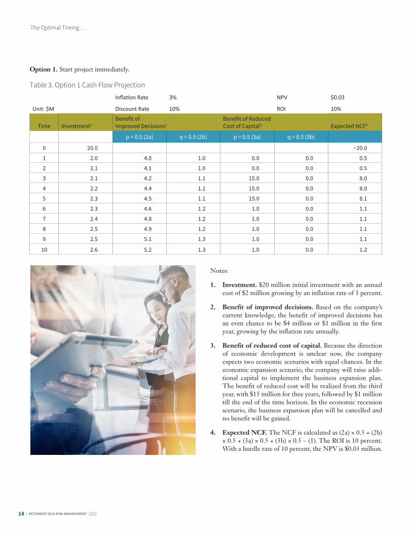
approach to assess risk exposure and calculate risk charges. The EC framework will be a major enhancement of the risk analysis in the company. The company will also use EC as an additional measure for capital management and performance measure-ment. The project is expected to require an initial investment of $20 million. Annual cost is expected to be $2 million inflated by 3 percent each year. Company ABC is considering whether and when to make the investment.
The benefits company ABC are looking for include:
• A contribution to the company’s enterprise risk manage-ment rating. The company plans to boost its credit rating in the medium term (three to five years) from A+ to AA−. ERM rating is an important component of risk assessment by rating agencies. By using the EC framework in business decision-making, the company wants to improve its risk man-agement practices.
• Improving business decision-making such as capital management, new business planning, risk optimization and performance measurement. Risk-adjusted return on economic capital will be used as a new measure. The benefit is measured by comparing the decision without the support of EC results and the decision with the support of EC results. In the past, the company had some successful and some unsuccessful capital management decisions. If the EC frame-work had been in place, some wrong decisions may have been corrected; however, correct decisions may have been changed as well. The net impact is seen as a benefit of the new project.
• Reducing the significant financing cost of a five-year business expansion plan. The company plans to issue bonds and shares at the same time. If the credit rating is upgraded, the company could save about 10 basis points in terms of the cost of capital rate. The EC model can also help the company understand the amount of capital it needs to raise to remain at the same level of capital adequacy. The additional information generated from the EC model may lead to a reduced level of required capital and therefore less capital cost. It may also lead to an increased level of capital needed. In this case, the future cost of capital raising or risk mitigation will be less after gain-ing a stronger capital position as indicated by the EC result.
As this is not a regulatory requirement, company ABC does not have to build the EC framework immediately. Several consider-ations on the timing are under review.
• The company wants to raise capital for the business expansion during an economic expansion to control the cost. Therefore, it is ideal that the EC framework building be finished before the capital raising and a future economic downturn. The economy has been recovering from the last financial crisis for six years and may keep expanding or move into a recession. If
the company starts the EC project now, it runs into the risk that the economy goes into a recession in the near future. The company will not implement the business expansion plan then and the benefit of the EC framework will be limited. In that case, the initial investment may be better used to improve the capital position rather than build the EC framework. On the other hand, if the company waits for six months or a year, the direction of the economy could be clearer and the company may be able to make a more informed decision. For example, the Federal Reserve has implemented the near-zero interest rate (0 to 25 basis points) policy for nearly seven years. A series of increases in the Fed rate would indicate an expanding econ-omy ahead. Keeping the rate unchanged or reducing it further would indicate a higher risk of economic recession. The Fed actively monitors the unemployment rate, inflation rate and economic activities to decide the rate level. There have been many discussions on rate hiking in 2015. In six months or a year, we may see a rate increase that raises the probability of a continuing economic expansion in the medium term. The company may decide to start the project immediately at that time. On the other hand, the average period of an economic cycle since World War II is seven years. An economic recession is also a possible scenario. If we experience a level rate or a rate decrease in the next six months or a year, the probability of an economic recession will be higher. In that case, the company may decide to postpone the project.
• The company does not have any experience with economic capital modeling and application. Without back testing and proper model validation, the EC result could be very sensitive to assumptions and misleading. In the 2008 financial crisis, some global insurance companies needed government bailout to survive although the economic capital result had showed these companies had strong capital positions and abundant free capital to deploy. Before the investment, the company may want to gain additional knowledge and experience to better assess the benefits of the EC framework.
• If the company wait for another six or 12 months for the EC project and then decide to build the EC framework, it may end up with an additional $10 million cost to achieve the target timeline of capital raising and business expansion. If interest rates are raised during that period, the financing cost will be higher as well.
With a 10-year time horizon, the following high level estimates of the costs and benefits are used for the timing decision.
To determine the optimal timing, the key is to evaluate how future information may improve future decisions.
14 | DECEMBER 2016 RISK MANAGEMENT
The Optimal Timing . . .
Notes:
1. Investment. $20 million initial investment with an annual cost of $2 million growing by an inflation rate of 3 percent.
2. Benefit of improved decisions. Based on the company’s current knowledge, the benefit of improved decisions has an even chance to be $4 million or $1 million in the first year, growing by the inflation rate annually.
3. Benefit of reduced cost of capital. Because the direction of economic development is unclear now, the company expects two economic scenarios with equal chances. In the economic expansion scenario, the company will raise addi-tional capital to implement the business expansion plan. The benefit of reduced cost will be realized from the third year, with $15 million for thee years, followed by $1 million till the end of the time horizon. In the economic recession scenario, the business expansion plan will be cancelled and no benefit will be gained.
4. Expected NCF. The NCF is calculated as (2a) × 0.5 + (2b) × 0.5 + (3a) × 0.5 + (3b) × 0.5 – (1). The ROI is 10 percent. With a hurdle rate of 10 percent, the NPV is $0.03 million.
Option 1. Start project immediately.
Table 3. Option 1 Cash Flow Projection
Inflation Rate 3% NPV $0.03
Unit: $M Discount Rate 10% ROI 10%
Time Investment1Benefit of Improved Decisions2
Benefit of Reduced Cost of Capital3 Expected NCF4
p = 0.5 (2a) q = 0.5 (2b) p = 0.5 (3a) q = 0.5 (3b)
0 20.0 −20.0
1 2.0 4.0 1.0 0.0 0.0 0.5
2 2.1 4.1 1.0 0.0 0.0 0.5
3 2.1 4.2 1.1 15.0 0.0 8.0
4 2.2 4.4 1.1 15.0 0.0 8.0
5 2.3 4.5 1.1 15.0 0.0 8.1
6 2.3 4.6 1.2 1.0 0.0 1.1
7 2.4 4.8 1.2 1.0 0.0 1.1
8 2.5 4.9 1.2 1.0 0.0 1.1
9 2.5 5.1 1.3 1.0 0.0 1.1
10 2.6 5.2 1.3 1.0 0.0 1.2

DECEMBER 2016 RISK MANAGEMENT | 15
Notes:
1. Investment. $25 million initial investment at time 1 with an annual cost of $2 million growing by the inflation rate, which is 3 percent.
2. Benefit of improved decisions. The benefit of improved deci-sions has an even chance to be $4.1 million or $1 million in the second year, growing by the inflation rate annually. At time 1, with the accumulation of knowledge and experience, the company will know exactly which benefit amount it will get.
3. Benefit of reduced cost of capital. Because the direction of economic development is unclear now, the company expected two economic scenarios with equal chances. In the economic expansion scenario, the company will raise additional capital to implement the business expansion plan. The benefit of reduced cost will be realized from the third year, with $15 million for three years, followed by $1 million till the end of the time horizon. In the economic recession scenario, the business expansion plan will be cancelled and no benefit will be gained. At time 1, the company will know exactly the scenario of the economy.
4. Expected NCF. The expected net cash flow is calculated as (2a) × 0.5 + (2b) × 0.5 + (3a) × 0.5 + (3b) × 0.5 – (1). It assumes that no matter what additional information the company will get in one year, it will still make the investment. The ROI is 5.4 percent. With a hurdle rate of 10 percent, the net present value is −$3.15 million. It is the NPV approach without considering the value of new information. If this approach is used, Option 1 will be chosen as it has a higher NPV and ROI.
5. NCF. Using the real option approach, at time 1, the com-pany gets to choose whether to make the investment or not. As shown in tables 4 and 5, items 5a to 5d are four scenarios and the company will know exactly which scenario will play out. The NCF of each scenario is the sum of correspond-ing benefits deducted by the investment. For example, the NCF of 5a = (2a) + (3a) – (1). Scenarios 5a and 5b will lead to a positive NPV. The investment will be made if 5a or 5b is expected at time 1. No investment will be made if 5c and 5d is realized. The aggregate NPV of Option 2 is $6.1 million (20.4 × 0.25 + 4.1 × 0.25). Compared to the NPV of Option 1, the company should wait one year before making the investment decision.
Option 2. Wait one year and then decide whether to make investment or not.
Table 4Option 2 Cash Flow Projection
Inflation Rate 3% NPV −$3.15 $20.37 $4.07 −$9.80 −$26.09
Unit: $M Discount Rate 10% ROI 5.4% 36% 17% −3% N/A
Time Invest-ment1Benefit of Improved Decisions2
Benefit of Reduced Cost of Capital3
Expected NCF4 NCF5a NCF5b NCF5c NCF5d
p = 0.5 (2a) q = 0.5 (2b)
p h= 0.5 (3a)
q = 0.5 (3b) Average p = 0.25
(2a)&(3a)p = 0.25 (2b)&(3a)
p = 0.25 (2a)&(3b)
p = 0.25 (2b)&(3b)
High Low High Low
Decision @ Time 1 Yes Yes No No
0 0.0 0.0 0.0 0.0 0.0
1 25.0 0.0 0.0 0.0 0.0 −25.0 −25.0 −25.0 −25.0 −25.0
2 2.1 4.1 1.0 0.0 0.0 0.5 2.1 −1.0 2.1 −1.0
3 2.1 4.2 1.1 15.0 0.0 8.0 17.1 13.9 2.1 −1.1
4 2.2 4.4 1.1 15.0 0.0 8.0 17.2 13.9 2.2 −1.1
5 2.3 4.5 1.1 15.0 0.0 8.1 17.3 13.9 2.3 −1.1
6 2.3 4.6 1.2 1.0 0.0 1.1 3.3 −0.2 2.3 −1.2
7 2.4 4.8 1.2 1.0 0.0 1.1 3.4 −0.2 2.4 −1.2
8 2.5 4.9 1.2 1.0 0.0 1.1 3.5 −0.2 2.5 −1.2
9 2.5 5.1 1.3 1.0 0.0 1.1 3.5 −0.3 2.5 −1.3
10 2.6 5.2 1.3 1.0 0.0 1.2 3.6 −0.3 2.6 −1.3

16 DECEMBER 2016 RISK MANAGEMENT
The Optimal Timing . . .
For simplicity, it is assumed that the company will know exactly the actual scenario at time 1 in this example. In reality, it is not realistic but the company may have a much better idea which scenario is the most likely one. It can be reflected by assigning a different probability than 25 percent for each scenario.
The costs, benefits and the value of new information vary from one risk management investment to another. They may not always be quantifiable and the uncertainty could be very high. Experts’ opinions are useful for choosing the best timing as well. For example, the company may not need one year extra time to better understand the benefit of improved decisions. Seeking the opinions of experts with relevant experience may shorten the knowledge gap.
7. CONCLUSIONThe timing of a risk management project could have a material impact on the cost, such as for a hedging program or the capital in a financing plan. Choosing the right timing to implement a risk management strategy or start an investment in new risk management functions is important.
Traditional approaches such as the NPV and real option approach used for investment decisions can be adjusted and used for timing decisions on risk management projects. The cost and benefit of a risk management project are different from a traditional investment. Risk management projects focus on more extreme scenarios than the expected cases.
Assessing the value of new information and its impact on future decisions is the key to timing decisions for risk management projects. The assessment usually requires comprehensive and complex analysis.
REFERENCESMeier, Ursina B., and J. François Outreville. 2003. “The Rein-surance Price and the Insurance Cycle.” Paper presented at the 30th seminar of the European Group of Risk and Insurance Economists (EGRIE), Zurich, September 2003. http://www.huebnergeneva.org/documents/Meier3.pdf.
Russo, J. Edward, and Paul J. H. Schoemaker. 1990. Decision Traps: Ten Barriers to Brilliant Decision-Making and How to Over-come Them. New York: Simon & Schuster.
Wang, Shaun S., John A. Major, Hucheng “Charles” Pan, and Jessica W. K. Leong. 2011. “U.S. Property-Casualty: Under-writing Cycle Modeling and Risk Benchmarks.” Variance 5 (2): 91–114. http://www.variancejournal.org/issues/05-02/91.pdf. n
ENDNOTE
1 VIX is a volatility index developed by the Chicago Board Options Exchange that tracks the implied volatility based on the prices of options on the S&P 500 index.
2 The VIX is used as the implied volatility for simplicity. In reality, the implied volatil-ity varies by option type (call or put), term of the option contract and the level of exercise price (in-the-money/at-the-money/out-of-the-money option).
3 Here ROI is the internal rate of return (IRR). It is the discount rate that makes the NPV equals to 0.
Kailan Shang, FSA, CFA, PRM, SCJP, is co-founder of of Swin Solutions Inc. He can be reached at [email protected].
Table 5 Investment Decision by Scenario
ScenarioBenefi t of Improved Decisions
Benefi t of Reduced Cost of Capital Probability Decision ROI NPV ($M)
5a High High 0.25 Yes 36% 20.4
5b Low High 0.25 Yes 17% 4.1
5c High Low 0.25 No −3% −9.8
5d Low Low 0.25 No N/A −26.1
Aggregate [(5a) and (5b) Only] $6.1

In Partnership with The Institutes
New: Become a Certified Specialist in Predictive Analytics (CSPA)
Learn more at TheCASInstitute.org
The CAS Institute is a subsidiary of the Casualty Actuarial Society (CAS) providing specialized credentials to quantitative professionals in the insurance industry.
Why a Credential from The CAS Institute?
SPECIALIZED
Our credential recognizes expertise in the highly
specialized area of predictive analytics for property and casualty
insurance applications.
RIGOROUS
Our credential leverages the integrity and relevance
of the CAS’s educational standards, which have been recognized globally for over
100 years.
IMPACTFUL
Our credential strengthens analytical teams by
providing resources and a practice community for the insurance industry’s
quantitative professionals.

18 DECEMBER 2016 RISK MANAGEMENT
Risk/Return, a Chimera?
By Sylvestre Frezal
In the short term, you don’t get the expected return—risk may be relevant, but expectation is not. In the long term, the risks offset and disappear—expectation is relevant, but risk is not. A decision is judged on a given temporal scale—either the short term or the long term. Then, when using risk/return, you rely on an inconsistent concept. Let’s clarify this point and its impacts.
A quantified optimization of risk/return is often considered as an investment best practice, both for asset managers, investment departments of insurers, or even considering the robo advisors proposed to non-professionals. Is this relevant? Does a quan-tified risk/return improve decision making? Does it provide objectivity? I do not think so.
THE QUANTITATIVE RISK/RETURN, AN OPERATIONALLY FALLACIOUS CONCEPTExpectation is what remains once the risks have mutualized, statistically offsetting each other—when considering a risk/expected return couple, the time horizon on which expectation can be observed is at least one order of magnitude longer than the one on which risk can be observed.
Figure 1
In other words, from an operational viewpoint, the quantified risk/return does not exist: either expectation is a good estimate of the result that we will get, meaning that the risk is negligible, or the risk is not negligible, meaning that expectation is signifi-cantly far from the result that we will get. If we want expectation to be concrete and meaningful, then risk has to be insignificant; and reciprocally, if the risk is significant, then expectation is totally virtual and has no concrete meaning. For example, if I know that at the end of the year, my stocks will either drop by 20 percent or raise by 30 percent and if I invest only till the end of the year, then I do not care about the fact that, in the long run, the stock return would be on average of either 4 percent or 7 percent. Concretely, expected return does not provide us an estimation on the return which we will actually get, even if you invest for 10 years. This can be observed in Table 1, an example of a gold return.
Table 1Gold Return Global Return Annual Return1960–1970 2% 0%1970–1980 1607% 33%1980–1990 -38% -5%1990–2000 -27% -3%2000–2010 339% 16%
The design flaw of the risk/expected return is that such a couple relies on a time horizon inconsistency. For a given deci-sion-maker, “risk” has a meaning at a timescale when “return” does not, and vice-versa. There is no timescale, at which risk and expectation both have an operational meaning.

DECEMBER 2016 RISK MANAGEMENT | 19
A QUANTIFIED RISK/RETURN DISTORTS OUR UNDERSTANDING OF THE SITUATIONAlthough expectation is not an estimate of the return which will actually be observed, it is generally perceived as such by the risk/return users—as a kind of “best estimate.” As a consequence, the decision-maker representation of the world is biased.
The decision maker was not able to forecast the future? Now he has two known, given figures; the two parameters being deter-mined, the world seems to be deterministic. The quantification made the feeling of randomness disappear. Paradoxically, people then tend to consider that (i) they should systematically get the expectation and that (ii) a risk which did not occur should not have been considered as a risk. (See sidebar.)
A TOOL WHICH CANNOT OFFER THE EXPECTED QUANTITATIVE OBJECTIVITYThe claimed ambition, the raison d’être, of the quantitative tools relying on risk/return is to objectivize the decision. In practice however, when the risk is significant, it is not possible to objectively calibrate a statistical indicator. Let’s take again the example of the expectation, and consider the DJ total return. Which time period shall we use? Shall we consider that we are in a post-financial crisis world? (9.9 percent) Shall we consider that our world is the world of the internet era? (2.3 percent) Shall we consider that nowadays economics is the one of the post oil-shock period? (9 percent) And if we had asked ourselves these questions in 2014 rather than 2016, the results would spread on a wider range: 12.8 percent, 1.5 percent and 6.1 percent.
Table 3DJ total return since … Seen at Year
End 2015Seen at Year
End 2013the financial crisis (01/2009) 9.9% 12.8%we entered the internet era (01/2000)
2.3% 1.5%
we live in the post oil-shocks economy (01/1982)
9.0% 6.1%
(source : dqydj.com)
Choosing between these different options requires an expert judgement; that is, by definition, a non-quantitatively objectiv-izable choice. Unfortunately, as it can be seen in Table 3, the dispersion between these expert judgements is wider than the dispersion between asset classes (just compare it to the US 10Y return over the period—depending on the time period chosen, it will be higher or lower). As a consequence, any final output relying on such input cannot be considered as quantitatively objective. The very purpose of the risk/return relying tools, i.e., quantitative objectivity, cannot be reached.
A TOOL WHICH DEGRADES GOVERNANCE AND DESTROYS ACCOUNTABILITY A governance issue then arises as subjectivity tends to become the prerogative of experts rather than the preserve of the deci-sion-makers. Senior managers are the ones who are entitled to activate their subjectivity. But using such tools leads to swap from an assumed subjectivity, located at the official decision-making level, towards a hidden subjectivity, actually concealed into the analysis level.
Furthermore, it will always be impossible to distinguish ex post between the modelled variability and a potential model error—nobody will ever be able to criticize the quality of the calibration; so experts are not accountable. And risk/return never excludes an adverse realization—the decision-maker choosing any allocation on the efficient frontier can always claim having chosen an optimal allocation without being accountable for any catastrophe, should it happen. In a nutshell, neither experts nor decision-makers are accountable—these tools offer nothing but an excellent formalization of “bad luck.”
SO WHAT? PROPOSING AN INTEGRATED (ANALYSIS-DECISION) TOOL UNDER THE DECISION-MAKER CONTROLRisk/return use is harmful in several ways: first, because it gen-erates a feeling of determinism and then damages the correct apprehension of the situation; second because it distorts the decision-making level through an oblivious transfer which
THE DIFFUSED AND PARADOXICAL FEELING OF A DETER-MINISTIC WORLD
i. When not getting expectation is perceived as abnormal
During an investment committee meeting, a CFO stated that “we have a higher level of risk than the market ...” and was straightforwardly interrupted by a critical business devel-opment executive “in this case, we should have a higher rate of return. I do not feel that’s the case ...”
ii. and not suffering from the risk realization too:
A leading industry lobbyist argued: “Can you imagine that following the currently selected criteria, those who sold their Apple stock three years ago to buy Greek debt would be exemplary according to Solvency II regulation?”
Of course, this feeling of a deterministic world leads to cruel disillusion, e.g., to the frequent reproach made to risk models which “did not anticipate the last crisis.”

20 DECEMBER 2016 RISK MANAGEMENT
Risk/Return, a Chimera?
prevents accountabilities identification. This calls for new asset allocation methodologies.
A scenario-based approach (see Figure 4) attempts to resolve these issues and leads to abandon the tender illusion of a quanti-tative objectivity provided by experts.
Figure 4
The three steps of a formal scenarios based optimization
1. Open the field of possible scenarios: identify the future scenarios that could be considered. (strong support of the experts to the decision makers)
2. Take responsibility on the strategic vision and risk taking: exclude from the previous list of scenarios these “in which we do not believe” or these which risk is accepted to be run (e.g., a default of U.S. government bonds?) (decision makers)
3. Optimize under constraint: maximize the return in the central scenario under the constraint of acceptance of the output in all the other not-excluded-scenarios. (experts)
scenarios to disregard—reintroduces stakeholder accountabil-ity and improves governance through an explicit and properly located subjectivity (step 2).
Such a methodological evolution modifies the positioning of the technical teams (quantitative ALM) regarding the executive management.
As a matter of fact, technical teams remain of the utmost impor-tance to focus the decision-maker’s attention toward possible scenarios which they would not have considered; to draw a typology of those scenarios so that they do not become too numerous to be cognitively handled by the decision-maker (step 1); to estimate impacts; and finally to optimize under constraint (step 3).
The technical teams will be much more exposed. The technical layer that allowed to dissolve their responsibility via the absence of falsifiability disappears. Furthermore, being the vehicles of the widening of the field of possible scenarios and the promot-ers of a random vision of the future, the technical teams become a source of anxiety for the executive management, where pre-viously, through their reality perception distorting tools, they were a tranquility center. However, they will benefit from an improved visibility and a more strategic positioning through deeper exchanges which will no longer be limited to an efficient frontier presentation. n
Sylvestre Frezal is the founder and co-director of the chair PARI (ENSAE ParisTech & Sciences Po), focusing on the apprehension of risks and dangers. He can be reached at [email protected].
Since several scenarios are considered, the fact that the deci-sion-maker does not know how markets will evolve materializes, and hence it reintroduces the feeling of randomness (step 1). The vision may be incomplete, a scenario can be wrongly neglected, but the perception of the very nature of the phe-nomenon is no more biased. Furthermore, the fact that the decision-makers chose the scenario to be considered—and what

2016 Joint Risk Management Research Update
2016 has been a busy year for Joint Risk Management Section research. To help the section council generate research to benefit its members, a dedicated group of
volunteers oversees the process—including managing the sec-tion’s research budget, establishing and implementing a research agenda and managing the studies that are pursued.
Once the research team has identified a topic area to undertake, a project team (POG) is recruited to manage the study—includ-ing defining the project scope, preparing solicitation materials to find a researcher, guiding the researcher to perform the study, and reviewing study deliverables. A POG was recently formed to investigate the feasibility of a study on negative interest rates. This study would examine how insurers are preparing for the possibility of sustained negative interest rates, the implications to the insurance industry of a sustained negative interest rate environment and how to adjust models to reflect negative inter-est rates. Systemically important financial institutions are also an area of study being considered.
Several projects are underway and in various stages. The follow-ing projects are in the early or middle states:
1. Country Risk Officer: This project will propose a frame-work for a country risk officer (CRO) and discuss the roles and responsibilities of a CRO. Sim Segal has recently been engaged to perform the research.
2. ERM Stakeholder Buy-in: Kailan Shang will identify the fac-tors, processes and practices that lead to both poor and strong levels of enterprise risk management stakeholder acceptance
3. 2016 ERM Emerging Risk Survey: The tenth survey in the series, Max Rudolph asks risk managers for their thoughts on emerging risks and identifies the trends across time. Look for the survey to be emailed to Joint Risk Management Section members by the end of the year.
4. Application of Enterprise Risk Management on National Long-Term Care Needs. This study continues to be defined and explores the impact at a national level of the application of enterprise risk management on Canadian long-term care needs.
5. Parameter Uncertainty. Brian Hartman and Robert Richard-son are developing a practical methodology for calculating parameter uncertainty for insurance risks.
While you wait for the results from the above studies to be released, there is plenty of recently released research to peruse. All the reports can be found on the SOA website.
1. 2015 Emerging Risk Survey results are now available. View the Max Rudolph authored report at:
https://www.soa.org/Research/Research-Projects/Risk-Manage-ment/2015-emerging-risks-survey.aspx
2. The 2016 ERM Symposium Monograph contains the research papers that were accepted for the 2016 ERM Sym-posium Call For Papers that helps strengthen the practice of enterprise risk management by opening new perspectives and expanding available insights, methods and tools.
https://www.soa.org/Library/Monographs/Other-Mono-graphs/2016/april/2016-erm-symposium.aspx
3. Policyholder Behavior in the Tail Risk Management Sec-tion Working Group UL with Secondary Guarantee 2015 Survey Results presents a range of assumptions actuaries use in pricing, reserving, and risk management of UL prod-ucts with secondary guarantees.
https://www.soa.org/Research/Research-Projects/Risk-Manage-ment/2015-pbitt-ul-secondary-guarantee.aspx
As this article illustrates, producing relevant research for its members is a priority of the Joint Risk Management Section Council and council members are interested in hearing from you. If you have an idea for a research project that would ben-efit Joint Risk Management Section members or would like to help with section research efforts, please contact Louise Francis, research lead for the section, at [email protected] or Ronora Stryker, SOA research actuary, at [email protected]. n
DECEMBER 2016 RISK MANAGEMENT | 21
22 | DECEMBER 2016 RISK MANAGEMENT
ORSA Process ImplementationBy Ger Bradley, Zohair Motiwalla, Padraic O’Malley and Eamonn Phelan
• Implementation
• Challenges faced by companies in the ORSA process
Based on survey results for those companies who’ve adopted the ORSA, it appears it may be having a positive impact. A few examples are:
• Over 80% of companies use an ORSA in key business decisions
• The ORSA seems to help level out the playing field from an ERM perspective
• Most companies view the costs associated with the ORSA as a very manageable element of their overall budgets.
This is just a snippet of findings, and other interesting obser-vations can be found within the full project report at http://www.soa.org/Research/Research-Projects/Risk-Management/research-2015-orsa-implementation.aspx.
SUMMARYThe ORSA (Own Risk and Solvency Assessment) for ERM frameworks and processes is continuing to be implemented by organizations.
In order to determine the popularity and degree to which this process is being used in business, a survey was conducted by a team from Milliman. The cross-disciplinary survey document was sent to companies around the world. The goal of the survey was to determine what insurance companies understood and expect from an ORSA, the effort to complete one, and the ben-efits from doing so.
The survey was broken out into five categories:
• Stress and scenario development processes
• Incentives, governance, and other behavioral aspects
• Evaluating the impact of the ORSA on a company’s overall results
• Evaluating the level of buy-in of the ORSA within an organization
• Board involvement
YOU MIGHT ALSO LIKE:2015 Emerging Risks Surveyhttps://www.soa.org/Files/Research/research-2015-emerging-risks-survey.pdf
Regulatory Risk and North American Insurance Organizations
https://www.soa.org/Files/Research/Projects/2015-reg-risk-com-pany-perspective.pdf
https://www.soa.org/Files/Research/research-2014-reg-risk.pdf n

DECEMBER 2016 RISK MANAGEMENT | 23
Estimating Probability of a Cybersecurity BreachBy Meghan Anthony, Maria Ishmael, Erik Santa, Arkady Shemyakin, Gary Stanull and Natalie Vandeweghe
Editor’s Note
Cyber risk management has been integrated into companies’ day-to-day operations. However, the evolving threats and fragmented data on cyber risk present a challenge for companies to understand and quan-tify a cybersecurity breach.
In this issue, we are pleased to share with readers a research paper from Professor Shemyakin and his team from University of St. Thomas on Estimating Probability of a Cybersecurity Breach. This article discusses how to estimate probability of a breach for a specific database applica-tion. In a simple example, the probability of a breach for a database with 100,000 records can be estimated by the probability of a database breach and a BF factor. The BF factor is derived from a predictive model as discussed below. This estimate would provide decision-makers information about the probability of a breach for a specific application, so to identify the most vulnerable applications, and make it possible to assign “risk ratings” on applications.
INTRODUCTIONInformation technology is the engine that drives the U.S. economy, giving it a competitive advantage in global markets by providing better services and facilitating greater productivity. This great value means that information systems are subject to a variety of threats, from malicious hackers to an employee simply losing a flash drive. Unfortunately, the threat landscape is constantly changing. To determine the risk these threats pose we need to evaluate the likelihood of their success in exploiting known and unknown vulnerabilities. This involves an accurate assessment of both impact and probability of breaches.
The purpose of this paper is to define a predictive model, based on known system attributes, for assessing risk associated with information systems. The goal is to provide decision-makers with the best possible information about the probability of a security breach so they can make informed decisions on how to best address the risk.
Most statistical papers dealing with cybersecurity are dedicated to analysis of the breach data and development of distribu-tion models for frequency of the breaches and severity of the associated losses. We will deal with a different problem: how
to estimate probability of a breach for a specific database application. This estimate would make it possible to assign “risk ratings,” allowing decision-makers to identify the most vulnerable applications based on some of their observable char-acteristics. However, obtaining such estimates will require us to build distribution models of these characteristics not only for “broken” applications, but also for “unbroken” ones.
To illustrate this point, let us consider an attribute A of an application (such as size, type of data, or the
industry). Using the Bayes formula, we may assess the proba-bility of an application with this attribute to be broken:
( ) ( / )( / ) ,( ) ( / ) ( ) ( / )
P B P A BP B AP B P A B P U P A U
=+ (1)
where ( )P B is overall prior probability of an application to be broken, ; while ( / )P A B and ( / )P A U are the probabilities to observe attribute A among broken and unbroken applications respectively. The latter two can be estimated from the historical data when such data are available. This estimation requires certain knowledge regarding the pop-ulation of unbroken applications, which is not typically used in analysis of the breach data.
PROBABILITY OF BREACH GIVEN APPLICATION SIZEFor an illustration let us concentrate on health-related data and single out such application attribute as record size measured as the total number of records. We will be considering the following grouping of application record sizes:
1S : Below 10,000
2S : 10,000–30,000
3S : 30,000–100,000
4S : 100,000–1 million
5S : Above 1 million
Suppose that independently of the application size, the probability of that to be breached (or broken) is estimated as
( )P B , the prior probability of a breach. Then the posterior probability of a breach conditional on the size of the class kS , where 1,2,3,4,5k = , can be evaluated as
(2)

24 | DECEMBER 2016 RISK MANAGEMENT
Estimating Probability of a Cybersecurity Breach
where ( / )kP S B and ( / )kP S U will be estimated from two different parametric distribution models for the random size BX of
a broken application and the size UX of an
unbroken application
Model selection using Akaike information criterion (AIC) brings about the results in Table 1.Table 1. AIC Values (the lower the better)
Model Normal Gamma WeibullXB 5964.4 5129.9 5117.2XU 435.5 479.3 447.6
Based on AIC values from Table 1 and graphs of ( )BF x in Figure 1 and ( )UF x in Figure 2, we recommend the choice
of Weibull distribution for both cases: with scale and shape estimated separately for models
via MLE:
BAYES FACTORSBased on the results from the previous section, we can estimate
( / )kP S B and ( / )kP S U . Obtaining posterior probabilities of a breach directly from Eq. (2) would require an additional specifi cation of the prior probability ( )P B , generally unknown. Therefore, we will use Bayes factors defi ned for each 1,...,5k = as
( / )( / )
kk
k
P S BBFP S U
=
It follows from Eq. (2) that for suffi ciently small ( )P B the Bayes factors approximate the ratios of probabilities and thus represent appropriate “adjustments” to prior probabilities of
DISTRIBUTION MODELS FOR APPLICATION SIZEFor the data on breaches, we used 1,572 data points recorded in the HHS database [2]. For the data on the unbroken appli-cations we used a sample size of 81 obtained from industry experience of application analysis from 2014 to 2015.
Application size is measured as the total num-
ber of records R log-transformed and shifted with natural thresholds 500 (minimum record size for broken data) and 10 (minimum record size for unbroken data) so that
For variables BX and UX three two-parameter distribu-tion models are considered: normal (Gaussian), suggested in Edwards, Hofmeyr and Forrest [1]; gamma; and Weibull. Maximum likelihood estimates (MLE) were obtained for all three models. In Figure 1 and Figure 2 the boundary of the shaded area corresponds to empirical CDF, the best normal fi ts are depicted by dashed lines, fi tted gamma in red and fi tted Weibull in green.
Figure 1. Distribution
0 5 10 15 20ln(Broken)
0.2
0.4
0.6
0.8
1.0CDF
Broken
Weibull Gamma Normal
Figure 2. Distribution
(3)
DECEMBER 2016 RISK MANAGEMENT | 25
• Analyze the Privacy Rights Clearinghouse dataset [6] to expand the scope of analysis to the industries beyond healthcare.
• Estimate risk to information systems based on the record size.
REFERENCES[1] Edwards, B., Hofmeyr, S., Forrest, S. (2015). Hype and Heavy Tails: A Closer Look at Data Breaches, http://www.econin-fosec.org/archive/weis2015/papers/WEIS_2015_edwards.pdf .
[2] United States Department of Health and Human Services (HHS), www.hhs.gov .
[2] Verizon Data Breach Incident Reports (DBIR), 2008 – 2016, www.verizonenterprise.com/verizon-insights-lab/dbir/.
[3] Symantec Healthcare Internet Security Threat Report (ISTR), 2016, www.symantec.com .
[4] Ponemon Institute 2015 Fifth Annual Benchmark Study on Privacy & Security of Healthcare Data, www.ponemon.org.
[5] HITRUST A Look Back: U.S. Healthcare Data Breach Trends 2012, hitrustalliance.net .
[6] Privacy Rights Clearinghouse Chronology of Data Breaches and Security Breaches 2005 – Present, www.privacyrights.org/. n
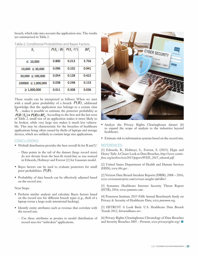
breach, which take into account the application size. The results are summarized in Table 2.
Table 2. Conditional Probabilities and Bayes Factors.Table 2. Conditional Probabilities and Bayes Factors.
These results can be interpreted as follows: When we start with a small prior probability of a breach ( )P B , additional knowledge that the application size belongs to a certain class
kS , makes it possible to estimate the posterior probability as , makes it possible to estimate the posterior probability as . According to the fi rst and the last rows
of Table 2, small size of an application makes it more likely to be broken, while very large size makes it much less vulnera-ble. This may be characteristic for the breaches of healthcare applications being often caused by thefts of laptops and storage devices, which are unlikely to contain large size applications.
CONCLUSIONS:• Weibull distribution provides the best overall fit for B and U
- Data points in the tail of the dataset (large record sizes) do not deviate from the best-fit trend-line as was noticed in Edwards, Hofmeyr and Forrest [1] for Gaussian model.
• Bayes factors can be used to evaluate posteriors for small prior probabilities ( )P B .
• Probability of data breach can be effectively adjusted based on the record size.
Next Steps:
• Perform similar analysis and calculate Bayes factors based on the record size for different breach types (e.g., theft of a laptop versus a large-scale intentional hacking).
• Identify entity attributes such as revenue that correlate with the record size.
- Use these attributes as proxies to model distribution of record sizes for “unbroken” applications.

26 | DECEMBER 2016 RISK MANAGEMENT
Estimating Probability of a Cybersecurity Breach
Gary Stanull, BS, MBA, MS, CISSP, CISM, is enterprise security architect at Optum Technology.He can be reached at [email protected].
Natalie A. Vandeweghe, University of St. Thomas, [email protected].
Meghan E. Anthony, University of St. Thomas, [email protected].
Maria L. Ishmael, University of St. Thomas, [email protected].
Erik W. Santa, University of St. Thomas, [email protected].
Arkady Shemyakin, Ph.D., is professor and director of statistics program at University of St. Thomas. He can be reached at [email protected].
DECEMBER 2016 RISK MANAGEMENT | 27
Cyber Risk is OpportunityBy Michael Solomon
Cybersecurity is what keeps our clients awake at night. Recent high-profile breaches have made it a boardroom concern. Whether as an endorsement to an existing pol-
icy or standalone, companies will look to their existing general liability provider for coverage and will not look kindly on those that refuse. Whether reading industry headlines or meeting with clients, cybersecurity is a key risk discussed. Actuaries must collaborate with other insurance industry experts to develop innovative, sustainable solutions for key stakeholders. This is how our internal and external clients will judge our value added.
This essay highlights the most important aspects of an actuary’s role in pricing cyber insurance.
Part 1 outlines the key risks of cybersecurity, why organiza-tions are looking to insure, why an insurance company will be required to write this business even with valid concerns, and available techniques for companies to manage risk.
Part 2 outlines the value actuaries are positioned to add.
Part 3 concludes that the growing need for this coverage rep-resents opportunity for actuaries.
PART 1: RISKDirect losses resulting from profit-motivated cybercrimes, such as ransoming data, are actually very low—approximately $2 billion to 3 billion per year—while direct and indirect costs of such crimes are very high. Defense costs for such crimes total approximately $19 billion per year, while indirect costs total an additional $40 billion per year. Costs of a breach can be in the billions (Table 1):
Many different costs are involved. Direct costs include the cost of ransomware, loss of data and lawsuits. Uninsured risk can lead to key people losing their jobs, and perhaps future cases will include boards being sued for negligence.
Table 1.High-Profile Data Breaches and Their Associated Costs
Breach Cause Cost (Ground Up) Cost (Insured)Epsilon Spear-phishing2 Up to $4 billion3 No coverage in place
Home Depot Vendor cybersecurity failure and Microsoft Windows security failure
$ billions4 $100 million
Wendy’s Unknown $ billions5 Unknown
Veterans Administration Computer/ external hard Drive incidentally stolen from employees house during burglary6
$500 million7 No coverage in place
Target Vendor cybersecurity failure $252 million8 $90 million
Hannaford Bros Malware $252 million9; ID theft insurance and replacement card costs held compensable10
No coverage in place
Sony PlayStation Unknown $171 million11 Unknown; settlement when appeal pending after bench granted summary judgment against Sony12
TJ Maxx Poorly secured wireless LAN in two stores13 $256 million14 $19 million15
Sony Pictures Entertainment North Korea $151 million + reputation $151 million
Heartland Payment Systems SQL injection attack16 $140 million17 $30 million18
Anthem Bogus domain name/ phishing Over $100 million19 $100 million20

28 | DECEMBER 2016 RISK MANAGEMENT
Cyber Risk is Opportunity
Figure 1Google Trends
IT vulnerabilities that have led to this state of affairs have shown almost no signs of improvement over time. Many organizations are “living below the security poverty line.” Cybersecurity bud-gets for many midsize and small companies are minimal. As a result, those companies often have little or no IT expertise, are unable to follow through on IT consultant recommendations and accordingly focus only on “putting out fires” rather than managing long-term cyber risk issues.21 Currently, there’s a gen-eral lack of objective proof that particular controls—policies, processes, technologies, and otherwise—have measurable and positive risk management impacts.22 Singapore is among the most technologically advanced countries in the world, yet its government’s cybersecurity solution is eliminating employees’ internet access.23
Limited technology solutions exist for addressing cyber risks. Most vendor options fall short of needed protection, and they don’t seem to be improving. Technical controls are often too complicated and/or costly for businesses to implement. The lack of available information about which cyber risks are most likely to materialize compounds these problems. Without more security intelligence, most organi-zations cannot make informed decisions about where to best spend their limited cybersecurity budgets. Given this land-scape, some companies may be inclined to buy cybersecurity insurance rather than spend money on technology solutions and other cybersecurity controls. They may opt to trans-fer risk entirely rather than invest in expensive and largely unproven cyber risk mitigation efforts. Without minimum underwriting requirements by carriers, this phenomenon could give rise to a moral hazard situation that encourages companies to take further risks rather than improve their cyber risk cultures.
There are companies offering cybersecurity endorsements for their general liability insureds without a full understanding of expected cost or coverage, instead relying on low policy limits. Would insureds not expect guidance on appropriate limits? When a loss occurs and the limits leave the insured with a large residual loss, will they keep any business with this company? Low loss limits are no substitute for actuarial diligence. Indeed, I argue below for generous limits.
PART 2: ADDING VALUEThere are two reasons insurers are offering coverage for cyber risk. First, general liability is a large, profitable business for many insurers. Insureds will test the markets if their current carrier cannot provide necessary coverages.
Second, cyber risk is a growing line of business, with potential to generate future revenue increases. Despite a recent appellate ruling that general liability policies can cover defense costs aris-ing from cyber breach,24 interest in cyber insurance continues to rise, as shown in Figure 1.25
Many of the risks that arise in cyberspace are not new (e.g., intellectual property theft, lost profits, privacy and reputational damages), and other professions are looking to actuaries to take the lead. Regarding a cyber incident data repository, a broker, two underwriters and a reinsurer suggested that actuaries are uniquely qualified to process this data to develop new, and enhance existing, cybersecurity insurance products.
It is precisely this absence of data where actuaries can demon-strate their value. We can itemize data items that should be collected for a meaningful analysis, comb through available data for frequency and severity benchmarks, determine what data are credible and appropriately weight differing indications. Furthermore, technologists are at a loss as to what protections work best. For example, how beneficial is encryption? What level should be adopted? Actuaries are uniquely skilled in finding answers to such questions in the data. By synthesizing available data, actuaries can guide insurers’ efforts to work with insureds to reduce losses and increase profitability.
Cybersecurity policies generally consist of multiple subcov-erages (e.g., Beazley’s Breach Response has eight26). Actuaries can determine the relative exposure from each of these sub-coverages and tailor the policy specifications to the insured’s concern.
One major issue in cyber insurance is what level of cybersecu-rity carriers should demand from the insured. If these levels are made too onerous, the marketability of the product will suffer. However, standards that are too lax will encourage insureds to skimp on expensive cyber protection solutions. Some have expressed the opinion that demanding the latest software patch updates from all employees is unreasonably onerous. In my opinion, it is not (Figure 2). The insured is in a position to ensure all employees are on a given patch at a given point in time through centralized updates. Insureds are also in a position
Source: Google Trends, “cyber insurance,” https://www.google.com/trends/explore#q=cyber%20insurance.
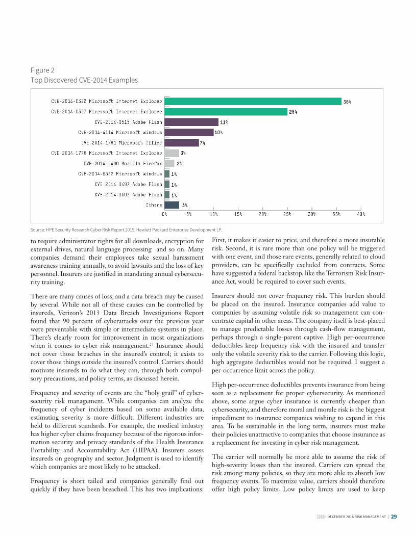
DECEMBER 2016 RISK MANAGEMENT | 29
to require administrator rights for all downloads, encryption for external drives, natural language processing and so on. Many companies demand their employees take sexual harassment awareness training annually, to avoid lawsuits and the loss of key personnel. Insurers are justified in mandating annual cybersecu-rity training.
There are many causes of loss, and a data breach may be caused by several. While not all of these causes can be controlled by insureds, Verizon’s 2013 Data Breach Investigations Report found that 90 percent of cyberattacks over the previous year were preventable with simple or intermediate systems in place. There’s clearly room for improvement in most organizations when it comes to cyber risk management.27 Insurance should not cover those breaches in the insured’s control; it exists to cover those things outside the insured’s control. Carriers should motivate insureds to do what they can, through both compul-sory precautions, and policy terms, as discussed herein.
Frequency and severity of events are the “holy grail” of cyber-security risk management. While companies can analyze the frequency of cyber incidents based on some available data, estimating severity is more difficult. Different industries are held to different standards. For example, the medical industry has higher cyber claims frequency because of the rigorous infor-mation security and privacy standards of the Health Insurance Portability and Accountability Act (HIPAA). Insurers assess insureds on geography and sector. Judgment is used to identify which companies are most likely to be attacked.
Frequency is short tailed and companies generally find out quickly if they have been breached. This has two implications:
First, it makes it easier to price, and therefore a more insurable risk. Second, it is rare more than one policy will be triggered with one event, and those rare events, generally related to cloud providers, can be specifically excluded from contracts. Some have suggested a federal backstop, like the Terrorism Risk Insur-ance Act, would be required to cover such events.
Insurers should not cover frequency risk. This burden should be placed on the insured. Insurance companies add value to companies by assuming volatile risk so management can con-centrate capital in other areas. The company itself is best-placed to manage predictable losses through cash-flow management, perhaps through a single-parent captive. High per-occurrence deductibles keep frequency risk with the insured and transfer only the volatile severity risk to the carrier. Following this logic, high aggregate deductibles would not be required. I suggest a per-occurrence limit across the policy.
High per-occurrence deductibles prevents insurance from being seen as a replacement for proper cybersecurity. As mentioned above, some argue cyber insurance is currently cheaper than cybersecurity, and therefore moral and morale risk is the biggest impediment to insurance companies wishing to expand in this area. To be sustainable in the long term, insurers must make their policies unattractive to companies that choose insurance as a replacement for investing in cyber risk management.
The carrier will normally be more able to assume the risk of high-severity losses than the insured. Carriers can spread the risk among many policies, so they are more able to absorb low frequency events. To maximize value, carriers should therefore offer high policy limits. Low policy limits are used to keep
Figure 2 Top Discovered CVE-2014 Examples
Source: HPE Security Research Cyber Risk Report 2015. Hewlett Packard Enterprise Development LP.

30 | DECEMBER 2016 RISK MANAGEMENT
Cyber Risk is Opportunity
premiums down when the insured is willing to risk high-severity losses, implicitly choosing to use their resources and capital to protect against other risks. Inadequate limits can lead to bank-ruptcy in the most severe cases. My experience is that insureds are not willing to accept the risk of high-severity losses from cybersecurity where the risks are not fully known. Carriers are in a much better place to accept this risk through the normal insurance risk-pooling mechanisms.
Another reason for policy limits is to keep the insured’s skin in the game. As outlined above, severity risk is significantly higher than frequency risk, so per-occurrence deductibles will be much more effective. Insureds are more able to retain the risk from high deductibles than low limits.
PART 3: CYBER RISK IS OPPORTUNITYI conclude that insurance companies can expand cybersecurity insurance offerings as follows:
Policies must contain austere per-occurrence deductibles and rigorous demands on insureds’ cybersecurity protection. This will keep premiums affordable while encouraging insureds to mitigate their risks.
• Limits should be generous on both per-occurrence and aggre-gate bases, since carriers are more able to assume the risk of high-severity losses than insureds, and there is limited oppor-tunity for insureds to minimize these low-frequency events.
• Coverages should be flexible to address insureds’ particular concerns.
While cyber risk is associated with some stunning losses, a lack of data and lack of consensus in the technology world as to how to treat it, this is precisely why actuaries’ specific skill set and experience can add value. As I write, the largest insurance com-panies are expanding their cyber liability teams,28 recognizing this coverage’s tremendous potential. Those who can solve the puzzles of cyber coverage and address their clients’ problems will be rewarded. Opportunity knocks! n
Michael Solomon, FCAS, CERA, MAAA, is a consulting actuary at The Actuarial Advantage, Inc. He can be reached at [email protected].
6 “Veterans Aff airs Data Theft ,” Electronic Privacy Information Center, n.d., https://epic.org/privacy/vatheft /. Retrieved June 8, 2016.
7 Supra note 4.8 Michael Kassner, “Data Breaches may Cost Less Than the Security to Prevent Them,”
Tech Republic, April 9, 2015, http://www.techrepublic.com/article/data-breaches-may-cost-less-than-the-security-to-prevent-them/. Retrieved June 8, 2016.
9 Widmer, “10 Most Expensive.”10 Decision and Order on Plaintiff s’ Revised and Supplemented Motion for Class
Certification, U.S. District Court, District of Maine (Portland), Civil Docket No.: 2:08-MD-1954-DBH, http://www.med.uscourts.gov/Opinions/Hornby/MDL/MDL1954_2013_03_20_ORDER11.pdf. Retrieved June 8, 2016.
11 Supra note 3.12 Young Ha, “Sony, Zurich Reach Settlement in PlayStation Data Breach Case in New
York ,” Insurance Journal, May 1, 2015, http://www.insurancejournal.com/news/east/2015/05/01/366600.htm. Retrieved June 8, 2016.
13 Jaikumar Vijayan, “One Year Later: Five Takeaways from the TJX Breach,” Com-puterworld, January 7, 2008, http://www.computerworld.com/article/2538711/cybercrime-hacking/one-year-later--five-takeaways-from-the-tjx-breach.html. Retrieved June 8, 2016.
14 Ross Kerber, “Cost of Data Breach at TJX Soars to 256m,” Boston Globe, August 15, 2007, http://archive.boston.com/business/globe/articles/2007/08/15/cost_of_data_breach_at_tjx_soars_to_256m/. Retrieved June 8, 2016.
15 “Insurance Company Reimburses TJX Almost $19 Million for Data Breach,” Fierce Retail, February 22, 2008, http://www.fierceretail.com/story/insurance-company-re-imburses-tjx-almost-19-million-for-data-breach. Retrieved June 8, 2016.
16 Jeremy Kirk, “Miami Man Indicted for Massive Credit Hack,” CSO Online, August 18, 2008, http://www.csoonline.com/article/2124294/malware-cybercrime/miami-man-indicted-for-massive-credit- hack.html. Retrieved June 8, 2016.
17 Supra note 8.18 Jaikumar Vijayan, “Heartland Breach Expenses Pegged at $140M—so Far,” Com-
puterworld, May 10, 2010, http://www.computerworld.com/article/2518328/cybercrime-hacking/heartland-breach-expenses-pegged-at-- 140m----so-far.html. Retrieved June 8, 2016.
19 Kassner, “Data Breaches.”.20 Mary A. Chaput, “Calculating the Colossal Cost of a Data Breach,” CFO, March 24,
2015, http://ww2.cfo.com/data-security/2015/03/calculating-colossal-cost-da-ta-breach/. Retrieved June 8, 2016.
21 Cyber Risk Culture Roundtable Readout Report, National Protection and Programs Directorate, U.S. Department of Homeland Security, Washington, DC, May 2013.
22 Supra note 21.23 “No Internet for Singapore Public Servants,” BBC News, June 8, 2016, http://www.
bbc.com/news/world-asia-36476422. Retrieved June 8, 2016.24 John P. Mello Jr., “Insurance Industry Buzzes Over Data Breach Ruling,” Tech News
World, April 21, 2016, http://www.technewsworld.com/story/83403.html. Retrieved June 14, 2016.
25 Google Trends, “cyber insurance,” https://www.google.com/trends/explore#q=cy-ber%20insurance. Retrieved June 9, 2016.
26 https://www.beazley.com/london_market/specialty_lines/professional_liability/technology_media_and_business_services/beazley_breach_response/under-standing_the_coverage.html. Retrieved June 14, 2016. Original data source: Breaches handled by Beazley Breach Response Services in 2014.
27 Cyber Risk Culture Roundtable Readout Report, National Protection and Programs Directorate, U.S. Department of Homeland Security, Washington, DC, May 2013.
28 Joyce Famakinwa, “Allianz Expands Cyber Insurance Team,” Business Insurance, June 7, 2016, http://www.businessinsurance.com/article/20160607/NEWS06/160609839?tags=58|285|93|137|98|83|76|71|70#utm_medium=email&utm_source=-bi-breakingnews&utm_campaign=bi-breakingnews-20160607. Retrieved June 9, 2016 (subscription required).
ENDNOTES1 Cybersecurity Insurance Workshop Readout Report, National Protection and Pro-
grams Directorate, U.S. Department of Homeland Security, Washington, DC, November 2012.
2 Jaikumar Vijayan, “Epsilon a Victim of Spear-phishing Attack, Says Report,” Comput-erworld, April 7, 2011, http://www.computerworld.com/article/2507075/security0/epsilon-a-victim-of-spear-phishing-attack--says- report.html. Retrieved June 8, 2016.
3 Lori Widmer, “The 10 Most Expensive Data Breaches,” Life Health Pro, June 18, 2015, http://www.lifehealthpro.com/2015/06/18/the-10-most-expensive-data-breaches?t=practice- management&slreturn=1465402403&page=5. Retrieved June 8, 2016.
4 Greg Masters, “Home Depot Breach Costs Expected to Reach Billions,” SC Media, October 2, 2015, http://www.scmagazine.com/home-depot-breach-costs-expect-ed-to-reach-billions/article/442849/. Retrieved June 8, 2016.
5 “Credit Unions Feeling Pinch in Wendy’s Breach,” Krebs on Security, March 2, 2016, http://krebsonsecurity.com/2016/03/credit-unions-feeling-pinch-in-wendys-breach/. Retrieved June 8, 2016.
DECEMBER 2016 RISK MANAGEMENT | 31
Recent Publications in Risk Management
As an ongoing feature in Risk Management, we will provide recent publications we find noteworthy to our readers. Please send suggestions for other publications you find
worth reading to [email protected], or [email protected].
1. 2015 Emerging Risks Survey CAS, CIA and SOA https://www.soa.org/Files/Research/research-2015-emerging-
risks-survey.pdf
2. Economic Scenario Generators - A Practical Guide SOA
https://www.soa.org/Files/Research/Projectsresearch-2016-eco-nomic-scenario-generators.pdf
3. 2016 Enterprise Risk Management Symposium Monograph
CIA, CAS, SOA and The Actuarial Foundation
https://www.soa.org/Library/Monographs/Other-Mono-graphs/2016/april/2016-erm-symposium.aspx
4. Evolving Challenges in Cyber Risk Management Oliver Wyman and the Marsh & McLennan Companies http://www.oliverwyman.com/content/dam/oliver-wyman/
global/en/2016/apr/Evolving%20challenges%20in%20cyber%20risk%20management.pdf
5. Waves of Disruption: The Cyber Risk threat to the Insurance Industry
Deloitte https://www2.deloitte.com/content/dam/Deloitte/ie/Documents/
FinancialServices/IE_2016_Cyber_Risk_Threat_to_Insurance_Industry.pdf
6. Issues Paper on Cyber Risk to the Insurance Sector International Association of Insurance Supervisors
http://www.iaisweb.org/page/consultations/closed-consultations/issues-paper-on-cyber-risks-to-the-insurance-sector/file/60062/issues-paper-on-cyber-risk-to-the-insurance-sector-public-consul-tation
7. Concept Proposal categorisation methodology for cyber risk
CRO Forumhttp://www.thecroforum.org/wp-content/uploads/2016/06/ZRH-16-09033-P1_CRO_Forum_Cyber-Risk_web.pdf n
Enterprise Risk ManagementHow do we govern it?www.cia-ica.ca/ERM
La gestion du risque d’entrepriseComment la gouverner ?www.cia-ica.ca/GRE

NONPROFIT ORGANIZATION
U.S. POSTAGE PAID
SAINT JOSEPH, MIPERMIT NO. 263
475 N. Martingale Road, Suite 600Schaumburg, Illinois 60173p: 847.706.3500 f: 847.706.3599 w: www.soa.org