joint removal implications thermal analysis and life …
TRANSCRIPT
Applied Research and Innovation Branch
JOINT REMOVAL IMPLICATIONS – THERMAL ANALYSIS AND LIFE-CYCLE
COST
Hussam Mahmoud, Ph.D.
Rebecca Atadero, Ph.D., P.E.,
Karly Rager, M.S.
Aura Lee Harper Smith, M.S.
Report No. CDOT-2018-12 April 2018

The contents of this report reflect the views of the
author(s), who is(are) responsible for the facts and
accuracy of the data presented herein. The contents
do not necessarily reflect the official views of the
Colorado Department of Transportation or the Federal
Highway Administration. This report does not
constitute a standard, specification, or regulation.

ii
Technical Report Documentation Page 1. Report No.
CDOT-2018-XX 2. Government Accession No.
3. Recipient's Catalog No.
4. Title and Subtitle
JOINT REMOVAL IMPLICATIONS – THERMAL ANALYSIS AND
LIFE-CYCLE COST
5. Report Date
April 2018
6. Performing Organization Code
7. Author(s)
Hussam Mahmoud, Rebecca Atadero, Karly Rager, Aura Lee Harper Smith
8. Performing Organization Report No.
CDOT-2018-12
9. Performing Organization Name and Address
Colorado State University Fort Collins, CO, 80523
10. Work Unit No. (TRAIS)
11. Contract or Grant No.
12. Sponsoring Agency Name and Address
Colorado Department of Transportation - Research 4201 E. Arkansas Ave. Denver, CO 80222
13. Type of Report and Period Covered
14. Sponsoring Agency Code
215.01
15. Supplementary Notes
Prepared in cooperation with the US Department of Transportation, Federal Highway Administration
16. Abstract
Deck joints are causing significant bridge deterioration and maintenance problems for Departments of Transportation
(DOTs). Colorado State University researchers partnered with the Colorado DOT to analyze the effects of temperature change
and thermal gradients on deck joint movement and provide recommendations regarding deck joint elimination. Typical steel
and concrete bridges were instrumented along the expansion joint and continuous data was collected for four months. In
addition, numerical finite element models and life cycle cost analysis were conducted to evaluate the potential for joint
elimination. The data indicates that temperature shifts and thermal gradients through the depth of the girders along the joint
are impacting the bridge’s movements and causing changes in stress. A strong parallel is shown between the temperature
changes and the study joint’s movement and changes in stresses in the girders. Despite being clogged, the joints showed some
movements, which corresponded to specific level of stresses in the adjacent girders, which was higher in the steel girders
than the concrete girders. The finite element results showed that a reduction in moment demand on the superstructure is not
apparent until a full-moment connection is utilized as a joint replacement. The parametric study and data analysis of thermal
gradients highlighted the need for further research on thermal gradients experienced by bridges. Finally, using the life cycle
cost analysis, it was concluded that elimination of joints would be the most cost-effective approach for minimizing the total
life cycle cost of the bridges. The modeling approach outlined in this study and the life cycle cost analysis framework can be
applied to any bridge and be used by CDOT to determine the viability of joint elimination for any bridge in CO. Implementation The results of this synthesis report will be used to inform the potential for joint elimination in bridges in Colorado.
17. Keywords
Deck Joints; Expansion Joint; Joint Elimination
Thermal Gradient; Bridges
18. Distribution Statement
This document is available on CDOT’s website http://www.coloradodot.info/programs/research/pdfs
19. Security Classif. (of this report)
Unclassified 20. Security Classif. (of this page)
Unclassified 21. No. of Pages
209 22. Price
Form DOT F 1700.7 (8-72) Reproduction of completed page authorized

iii
ACKNOWLEDGEMENT
The authors wish to thank the CDOT Applied Research and Innovation Branch for funding this
study. The authors acknowledge the project panel for providing valuable technical discussion and
guidance throughout the project period. The time, participation and feedback provided by the
project panel members: Jessica Terry, Trever Wang, Behrooz Far, Thomas Kozojed, Joe Jimenez,
Kane Schneider, and Matthew Greer, are greatly appreciated.

iv
EXECUTIVE SUMMARY
Bridge expansion joints are a particularly troublesome component of bridges and many
Departments of Transportation (DOTs) are looking for a solution to deteriorating expansion joints
on highway bridges. Bridge expansion joints create a break in the structural continuity of a bridge
allowing clogging gravels and corroding chlorides to enter. They are designed to absorb thermal
movements of the bridge between two bridge elements. There are three main issues regarding
expansion joints: maintenance, knowledge about thermal movements, and costs.
In order to prevent deterioration due to expansion joints, the joints must be cleaned
regularly and replaced promptly after failure. However, most DOTs do not have the personnel,
time or resources to maintain expansion joints in their districts which leads to bridge deterioration.
Other similar maintenance and component issues have been addressed using a Life-Cycle Cost
Analysis (LCCA). For this to be used on expansion joints the three main issues of thermal
knowledge, maintenance, and costs must first be addressed.
The main goals of this project are to 1) expand understanding of thermal loading effects on
bridge expansion joints and 2) conduct a LCCA for joint elimination and retrofits for bridges in
Colorado. These objectives were accomplished utilizing data from in field instrumentation and
finite element models. The study has been developed jointly between the Colorado Department of
Transportation (CDOT) and researchers at Colorado State University
Three main tasks were conducted to achieve the objectives: 1) collect and analyze long-
term thermal loading data from existing bridges to assess thermal loading impacts on joints; 2)
perform a parametric study using a calibrated finite element model to further understanding of

v
joint behavior and retrofit options under thermal loads; 3) perform a LCCA for bridge expansion
joint retrofitting including impacts on bridge superstructure.
The significance of this work includes the results of data collection and analysis, the
parametric studies, and the LCCA findings. The results of the numerical analysis show that
clogged joints induce some localized stress, more so for the steel bridge, but do not significantly
affect the global performance of the superstructure. The results also show that a reduction in
moment demand on the superstructure is not apparent until a Full-Moment connection is utilized
as a joint replacement. The parametric study and data analysis of thermal gradients indicate a stark
need for further research into thermal gradients experienced by bridges. Finally, the LCCA
concluded that a retrofit continuous bridge design would provide the most cost-effective design by
decreasing joint replacement costs and pier cap corrosion. The modeling approach outlined in this
study and the life cycle cost analysis framework can be applied to any bridge and be used by CDOT
to determine the viability of joint elimination for any bridge in CO.
vi
TABLE OF CONTENTS
Acknowledgement ......................................................................................................................... iii
Executive Summary ....................................................................................................................... iv
LIST OF TABLES ......................................................................................................................... ix
LIST OF FIGURES .........................................................................................................................x
CHAPTER 1 INTRODUCTION ..................................................................................................1
1.1 Statement of the Problem .......................................................................................1 1.2 Objectives and Scope of Research .........................................................................3
CHAPTER 2 BACKGROUND AND LITERATURE REVIEW ..............................................5
2.1 Introduction ............................................................................................................5
2.2 Girder to Abutment Consideration .........................................................................5 2.3 Leading Agencies...................................................................................................7
2.3.1 Tennessee Department of Transportation ......................................................7
2.3.2 Transportation Ministry of Ontario ................................................................8 2.3.3 Colorado Department of Transportation ........................................................8
2.4 Types of Retrofit Connections ...............................................................................9
2.5 Thermal Effects on Bridges .................................................................................10
2.6 Increasing Popularity ...........................................................................................12 2.7 Global Bridge Performance .................................................................................13
2.7.1 Longitudinal Movement...............................................................................13 2.7.2 Effects of Bridge Geometry (Skew and Curvature) .....................................16 2.7.3 Potential Increase in Moment Capacity .......................................................18
2.8 Local Superstructure Behavior ............................................................................18 2.8.1 Corrosion......................................................................................................19
2.8.2 Blocked Expansion ......................................................................................20 2.8.3 Lateral Torsional Buckling Risk for Steel Girders ......................................22 2.8.4 Temperature Gradient ..................................................................................23 2.8.5 Temperature Data.........................................................................................28
2.8.6 Influence of Temperature compared to other variables ...............................29 2.9 LCCA Process ......................................................................................................30 2.10 Components of LCCA .........................................................................................34
2.11 Components and Parameters Related to Bridge Maintenance .............................37 2.12 Maintenance of Bridges with Expansion Joints ...................................................42 2.13 Current LCCA Models for Bridges......................................................................50 2.14 Conclusion ...........................................................................................................58
CHAPTER 3 BRIDGE SELECTION AND FIELD INSTRUMENTATION PLAN ............61

vii
3.1 Introduction ..........................................................................................................61
3.2 Steel Bridge (B-16-FM) .......................................................................................62 3.3 Reinforced Concrete Bridge (C-17-AT) ..............................................................67
3.4 Field Instrumentation ...........................................................................................69 3.4.1 Strain Gages .................................................................................................74 3.4.2 Thermocouples .............................................................................................77 3.4.3 Linear Potentiometers ..................................................................................78 3.4.4 Wires ............................................................................................................81
3.4.5 The Data Acquisition System ......................................................................83 3.5 Remote Data Collection .......................................................................................85 3.6 Solar Panel Installation ........................................................................................87
CHAPTER 4 CONTROLLED LOAD TEST MODEL VALIDATION .................................90
4.1 Introduction ..........................................................................................................90 4.2 Test Vehicle Information .....................................................................................90
4.3 Model and Predictions .........................................................................................91 4.4 Results and Comparison to the Finite Element Models .......................................92
4.4.1 C-17-AT .......................................................................................................92
4.4.1 B-16-FM ......................................................................................................94
CHAPTER 5 DATA ANALYSIS FOR BRIDGE C-17-AT .....................................................96
5.1 Introduction ..........................................................................................................96 5.2 Analysis Plotting Code ........................................................................................96 5.3 Sensor Correlation and Patterns ...........................................................................97
5.4 Thermal Gradients and Bridge Deterioration ....................................................104
5.5 Summary and Preliminary Conclusions.............................................................109
CHAPTER 6 PARAMETRIC STUDY for C-17-AT ..............................................................111
6.1 Introduction ........................................................................................................111
6.2 CSiBridge Finite Element Numerical Model .....................................................111 6.3 Joint Retrofitting Options Analyzed ..................................................................113
6.4 Joint Clogging Stiffness Considered ..................................................................117 6.5 Parametric Analysis Matrix ...............................................................................117 6.6 Analysis Results and Implications .....................................................................118
6.6.1 Clogged Joint Results and Implications .....................................................119 6.6.2 Joint Retrofit Connection Results and Implications ..................................124
6.7 Conclusion .........................................................................................................127
CHAPTER 7 PARAMETRIC STUDY for B-16-fm ...............................................................129
7.1 Introduction ........................................................................................................129 7.2 B-16-FM: Steel Plate Girder Bridge with Concrete Slab ..................................130 7.3 CSi Bridge Model Methodology ........................................................................133
7.3.1 Shell and Frame Elements .........................................................................134 7.3.2 Composite Behavior...................................................................................134 7.3.3 Thermal Analysis .......................................................................................135

viii
7.3.4 Boundary Conditions .................................................................................135
7.4 Joint-Removing Connection Types Considered ................................................137 7.5 Thermal Gradients Considered ..........................................................................137
7.6 Connection Link Stiffness Considered ..............................................................138 7.7 Parametric Study Matrix and Overview ............................................................139 7.8 Results ................................................................................................................140
7.8.1 Effect of Clogged Joints.............................................................................141 7.8.2 Effect of Connection Types .......................................................................148
7.9 Conclusion .........................................................................................................155
CHAPTER 8 LIFE-CYCLE COST ANALYSIS ....................................................................156
8.1 Life-Cycle Cost Analysis Model .......................................................................156 8.2 Life-Cycle Cost Analysis Equations and Variables ...........................................157
8.3 Cost Scenario Equations, Variables, and Calculations ......................................160 8.3.1 Cost Scenario 1 ..........................................................................................161
8.3.2 Cost Scenario 2 ..........................................................................................162 8.4 Results ................................................................................................................166
8.4.1 Cost Scenario 1 Results .............................................................................166
8.4.2 Cost Scenario 2 Results .............................................................................168 8.5 Conclusion .........................................................................................................168
CHAPTER 9 SUMMARY AND CONCLUSIONS .................................................................170
9.1 Summary ............................................................................................................170 9.2 Significance and Further Research ....................................................................171
REFERENCES ............................................................................................................................173
APPENDIX A. INSTRUMENTATION PLAN FOR C-17-AT ................................................177

ix
LIST OF TABLES
Table 2-1 Parameters Assumed for User Cost Computation (Kim et al., 2010) .......................... 42 Table 2-2 A Risk Interaction Matrix (Agency and Severn, 2000) ............................................... 54 Table 2-3 Risk interaction matrix for Example (Agency and Severn, 2000) ............................... 55 Table 4-1. Comparison of Field Stress and Model Stress Predictions .......................................... 93
Table 4-2. Comparison of Field Stress to Modeled Stress Predictions......................................... 95 Table 5-1 Temperature and Force for C-17-AT and B-16-FM ................................................... 108 Table 8-1 Assumed Costs Based on CDOT Data (Colorado Dept. of Transportation 2016) ..... 159 Table 8-2 Test Matrix Considering Agency and Bridge Dependent Variables .......................... 160 Table 8-3. LCC for Cost Scenario 1 .......................................................................................... 166
Table 8-4. LCC for Cost Scenario 2 .......................................................................................... 168

x
LIST OF FIGURES
Figure 2-1. Maximum Expected Temperature for Steel Bridges with Concrete Decks ............... 14 Figure 2-2. Debris in expansion joint in service for less than six months (Chen, 2008) .............. 20 Figure 2-3. Cycles of Pavement Growth (Rogers and Schiefer, 2012) ........................................ 22 Figure 2-4. Vertical Temperature Distributions of Heating of Steel Composite Girders (Chen,
2008) ............................................................................................................................ 27 Figure 2-5. Vertical Temperature Distributions of Cooling of Steel Composite Girders (Chen,
2008) ............................................................................................................................ 27 Figure 2-6 Life-Cycle Cost Analysis Process Flow Chart ............................................................ 32 Figure 2-7 Life-Cycle Cost Analysis Costs Flow Chart ............................................................... 35
Figure 2-8 Life-Cycle Cost Analysis Costs Flow Chart for Bridges ............................................ 40 Figure 2-9 Factors affecting MR&R Costs for Bridges ................................................................ 44
Figure 2-10 Section Thru Strip Seal Bridge Expansion Device (CDOT, 2015) ........................... 47 Figure 2-11 Types of Joints ( Lima and de Brito, 2010) .............................................................. 48
Figure 2-12 Life-Cycle Cost Analysis Models for Bridges .......................................................... 52 Figure 2-13 MR&R action severity vs Bridge Age ...................................................................... 56
Figure 3-1. Plate Girders for Bridge B-16-FM (Google Maps Image) ......................................... 63 Figure 3-2. B-16-FM Superstructure from the West Abutment (photo by Authors) .................... 64 Figure 3-3. View of B-16-FM from East Abutment (Photo courtesy of CDOT) ......................... 65
Figure 3-4. Finger Joint Clogged by Debris on B-16-FM (Photo courtesy of CDOT) ................ 66 Figure 3-5. Aerial View of C-17-AT (Photo courtesy CDOT) ..................................................... 67
Figure 3-6. C-17-AT (Photo courtesy CDOT) .............................................................................. 68 Figure 3-7. Discoloration under expansion joint on C-17-AT (Photo courtesy CDOT) .............. 69
Figure 3-8 C-17-AT Overview ................................................................................................... 70 Figure 3-9 C-17-AT Sideview .................................................................................................... 71
Figure 3-10 C-17-AT Underside – Corrosion & Leakage ............................................................ 71 Figure 3-11 C-17-AT Expansion Joint Clogging ......................................................................... 72 Figure 3-12 C-17-AT Expansion Joint Deterioration ................................................................... 73
Figure 3-13 C-17-AT Expansion Joint Sensor Placement ............................................................ 74 Figure 3-14 Concrete Strain Gage ................................................................................................ 75
Figure 3-15 Strain Gage Application ............................................................................................ 76 Figure 3-16 Strain Gage Protection .............................................................................................. 76 Figure 3-17 Thermocouple Application ........................................................................................ 78 Figure 3-18 Thermocouple Connectors ........................................................................................ 78 Figure 3-19 Extended Linear Potentiometer ................................................................................. 79
Figure 3-20 Linear Potentiometer Mount ..................................................................................... 80 Figure 3-21 Linear Potentiometer in Place on Joint ..................................................................... 81
Figure 3-22 PVC covered Linear Potentiometer .......................................................................... 81 Figure 3-23 Shielded Thermocouple Wire ................................................................................... 82 Figure 3-24 Double Shielded Wire ............................................................................................... 83 Figure 3-25 Job Box on North Abutment’ .................................................................................... 84 Figure 3-26 DAQ in Job Box ........................................................................................................ 84 Figure 3-27 Wires Along Railing ................................................................................................. 85

xi
Figure 3-28 RavenTXV Modem ................................................................................................... 86
Figure 3-29 Modem Antenna ........................................................................................................ 87 Figure 3-30 Solar Panel, 70 Watt .................................................................................................. 88
Figure 3-31 Solar Panel Frame ..................................................................................................... 89 Figure 3-32 Solar Panel Attached to Abutment ............................................................................ 89 Figure 4-1 Aspen Aerials A-40 Truck with Dimensions and Axel Weights ................................ 91 Figure 4-2 Front Axle Control Load Test Data ............................................................................ 92 Figure 4-3 Back Axle Control Load Test Data ............................................................................. 93
Figure 4-4. Field Control Load Test with Front Axle of A-40 Truck at Mid-Span ...................... 94 Figure 4-5. Field Control Load Test Microstrain with Back Axles at Mid-Span ......................... 95 Figure 5-1 C-17-AT Bridge Sensor Data Oct.15th through Oct. 30th, 2016 .................................. 99 Figure 5-2 C-17-AT Bridge Sensor Data Nov.30th through Dec. 2nd, 2016 ............................... 100 Figure 5-3 C-17-AT Bridge Sensor Data Oct.15th through Oct. 18th, 2016 ................................ 101
Figure 5-4 B-16-FM Bridge Sensor Data Sept. 7th through Oct. 11th, 2016 ............................... 102 Figure 5-5 Maximum Temperature Difference Through Depth vs Stress Data. ........................ 104
Figure 5-6 Design Standard vs. Measured Temperature Gradients. ........................................... 105 Figure 5-7 Deterioration of C-17-AT Abutments and Joints ...................................................... 107
Figure 5-8 Deterioration of B-16-FM Abutments and Joints ..................................................... 107 Figure 6-1 C-17-AT Finite Element Model. ............................................................................... 112
Figure 6-2 C-17-AT Finite Element Model Ties Between Girder and Slab ............................... 112 Figure 6-3 (a) AASHTO Thermal Gradient, (b) New Zealand Thermal Gradient. .................... 115 Figure 6-4 Piece-wise Approximation: (a) AASHTO Thermal Gradient, (b) New Zealand
Thermal Gradient, (c) Uniform Gradient ................................................................... 116 Figure 6-5 Parametric Study Matrix ........................................................................................... 118
Figure 6-6 AASHTO HS20-44 Truck (Precast/Prestressed Concrete Institute, 2003) ............... 119 Figure 6-7 Maximum Stress in Bottom of Girder at End ........................................................... 120
Figure 6-8 Maximum Stress in Bottom of Girder at Mid-span .................................................. 121 Figure 6-9 Maximum Stress in Top of Girder at Mid-span ........................................................ 122
Figure 6-10 Maximum Stress in Top of Girder at the Ends ....................................................... 122 Figure 6-11 Stress Demand in Bottom of Girder at Mid-span due to Moment resulting from the
Truck Load ................................................................................................................. 123
Figure 6-12 Moment Demand Due to Thermal and Truck Load in Bottom of Girder at Mid-span
.................................................................................................................................... 124
Figure 6-13 Maximum Stress at Bottom of Girder due to Thermal Gradients Only .................. 125 Figure 6-14 Maximum Stress at Bottom of Girder due to Truck Loading Only ........................ 126 Figure 6-15 Maximum Stress at Bottom of Girder due to Thermal Gradients and Truck Load
Combined ................................................................................................................... 127 Figure 7-1. Plate Girders in Construction Documents for Bridge B-16-FM (Courtesy CDOT) 130
Figure 7-2. Plate Girders for Bridge B-16-FM ........................................................................... 131 Figure 7-3. Slab Geometry described in the Construction Documents ...................................... 132
Figure 7-4. Finite Element Model Illustration of super-elevation described in the Construction
Documents ................................................................................................................. 132 Figure 7-5. Extruded View of B-16-FM Superstructure ............................................................. 133 Figure 7-6. Alternative view of B-16-FM Bridge Model (unstressed, unloaded state) .............. 133 Figure 7-7. Nodes pinned to simulate pinned boundary condition at support ............................ 136 Figure 7-8. Girder Stress Distribution under Self-Weight Showing Shear Lag Behavior .......... 136
xii
Figure 7-9. Parametric Study Matrix .......................................................................................... 139
Figure 7-10. AASHTO HS20-44 Truck (Precast/Prestressed Concrete Institute, 2003) ............ 140 Figure 7-11. Compressive Stress at Bottom of Girder ................................................................ 142
Figure 7-12. Compressive Stress at Bottom of Girder (Normalized) ......................................... 143 Figure 7-13. Local Compressive Stress in Deck due to Thermal Loading ................................. 144 Figure 7-14. Local Compressive Stress in Deck due to Thermal Loading (Normalized) .......... 145 Figure 7-15. Tensile Stress at Bottom of Girder due to Only Truck Loading ............................ 146 Figure 7-16. Stress at Bottom of Girder under the Truck Load due to Thermal and Truck Loading
.................................................................................................................................... 147 Figure 7-17. Stress at Bottom of Girder due to Thermal and Truck Loading (Normalized) ...... 148 Figure 7-18. Compressive Stress at Bottom of Girder due to Only Thermal Loading ............... 149 Figure 7-19. Compressive Stress at Bottom of Girder due to Only Thermal Loading
(Normalized) .............................................................................................................. 150
Figure 7-20. Local Compressive Stress in Concrete Deck due to Only Thermal Loading ........ 151 Figure 7-21. Local Compressive Stress in Concrete Deck due to Only Thermal Loading
(Normalized) .............................................................................................................. 151 Figure 7-22. Tensile Stress at Bottom of Girder due to Only Truck Loading ............................ 152
Figure 7-23. Tensile Stress at Bottom of Girder due to Only Truck Loading (Normalized) ..... 153 Figure 7-24. Stress at Bottom of Girder due to Thermal and Truck Loading ............................ 154
Figure 7-25. Stress at Bottom of Girder due to Thermal and Truck Loading (Normalized) ...... 154 Figure 8-1 LCCA Cost Scenario ............................................................................................... 157 Figure 8-2 Life 365 Chloride Surface Concentration Vs. Time (years) for Colorado ............... 165

1
CHAPTER 1
INTRODUCTION
1.1 Statement of the Problem
Degradation of United States’ public infrastructure has attracted attention from the public
and governing agencies alike. A challenge facing transportation departments is management of
leaking and clogged expansion joints in bridge structures, which result in significant deterioration
to bridge substructures and superstructures. The need for a different maintenance strategy or a new
solution to bridge expansion joints is ever pressing.
Bridge expansion joints create a break in the structural continuity of a bridge. They are
designed to absorb thermal movements of the bridge between two bridge elements. Notably,
expansion joints, and bearings, require regular maintenance throughout their life-span in order to
function properly and thus inhibit damage to the bridge superstructure (Hawk, 2003). A clogged
joint can induce un-designed for stresses into the girders and abutments. A leaking joint can
introduce corrosion into the superstructure below, primarily the pier caps (Lam et al., 2008).
Deicing salts and chemicals used in colder regions increase the likelihood of corrosion beginning
in the superstructure if a leaking joint is present. Additionally, bridges located in the mountains,
where chains are used on vehicles, can experience deterioration that is more extensive. These
issues are what caused expansion joints to be named by the American Association of State
Highway and Transportation Officials (AASHTO) as the second most common bridge
maintenance issue behind concrete bridge decks (AASHTO, 2012).

2
There are three main issues regarding expansion joints: maintenance, knowledge about
thermal movements, and costs. Expansion joints are very susceptible to a lack of maintenance due
to DOTs lacking the people and resources to maintain their numerous bridge expansion joints
regularly. A bridge expansion joint needs to be cleaned regularly, once every few months and
repair to protect it from clogging and leakage due to a damaged or worn out seal. However, this
type of maintenance is beyond the scope of DOTs, and consequently removing the expansion joints
from existing bridges altogether might solve this maintenance issue. The second issue is a lack of
current research on thermal effects on bridge joints, including how much movement is induced by
thermal loads, and how much stress. Without knowing how important expansion joints are to
bridge behavior, bridge movement and stress, it is hard to know how removing the expansion joints
would affect the overall structure. Finally, costs are an issue that needs addressing. Costs are
important in any long-term decision such as this one. DOTs need to know what makes the most
economic sense regarding expansion joints. The economic issue could be addressed utilizing a life-
cycle cost analysis (LCCA) in conjunction with data analyzing the effects of temperature on joint
behavior. Consequently, a more cost-effective solution could be obtained for the issue of
deteriorating expansion joints in existing bridges that does not require frequent extensive
maintenance and uses knowledge of thermal effects.
The use of LCCA in infrastructure design, maintenance, and repair is becoming more
prevalent around the U.S. as well as around the world. The public is becoming more interested in
how officials use tax dollars, and thus encouraging agencies to look into and utilize better methods
of infrastructure analysis for higher cost efficiency (Al-Wazeer et al., 2005; Ozbay et al., 2004).
Stanford University defines LCCA concisely when they say it is the "process of evaluating the
economic performance of a building [or other piece of infrastructure] over its entire life"

3
(University, 2005). A LCCA of expansion joints on existing bridges in this manner could build
on results of data regarding thermal behavior of bridge joints.
1.2 Objectives and Scope of Research
The overall goal of this study is to increase understanding of thermal loading and
movement that is exhibited by bridges in Colorado and to provide recommendations for the
elimination of deck joints in existing bridges. Specific objectives of this goal were developed
through discussion and coordination between researchers at Colorado State University (CSU) and
the Colorado Department of Transportation (CDOT). Four main tasks were identified. The tasks
include: 1) collection long-term thermal loading data to assess joint movement of two bridges; 2)
development and validation of finite element models of one steel bridge and one concrete bridge;
3) assessment of joint elimination options; and 4) assessment of the life-cycle cost and the
implications associated with joint removal.
The long-term data collected in Task 1 can provide information to CDOT about the actual
movement of the selected bridges and joints. This can then be compared to the deck joint
movement and thermal loading requirements outlined in the AASHTO LRFD Bridge Design
Specifications. Development of the finite element models in Task 2 can help assess the stresses
induced in the bridge from different connection types and thermal loading scenarios. Development
of retrofit connection types in Task 3 can provide CDOT with options to eliminate deck joints in
bridges with confidence. Assessment of the life cycle cost (LCC) implications in Task 4 can help
CDOT make decisions about which bridges to retrofit to eliminate deck joints and when a joint
eliminating retrofit is the most appropriate option. The content of this report includes:

4
- A literature and background review
- Bridge selection and field instrumentation
- Load-controlled tests for validating the finite element models
- Parametric studies analyzing the joints response to different clogging stiffness,
thermal gradients, and retrofit options
- LCCA of bridge expansion joints and retrofitting.

5
CHAPTER 2
BACKGROUND AND LITERATURE REVIEW
2.1 Introduction
To achieve a thorough understanding of the problem and the state of the current research
relating to the elimination of deck joints, an extensive literature review was performed. Topics
such as origins of code provisions, local behavior at joints, global bridge performance, leading
agencies in the field, thermal loads, and LCCA are included in this chapter.
2.2 Girder to Abutment Consideration
Various structural systems have been developed to allow for thermal movements while
reducing or eliminating deck joints. Placing the joints at the ends of approach slabs or only at the
abutments is one method used. Allowing rotation of the abutments is another method that has been
utilized. This section aims to discuss these differences and the nomenclature that has been put into
place by the transportation agencies.
Integral bridges are bridges without deck joints (AASHTO LRFD Bridge Design
Specifications, 2012) and have been increasingly used in recent years by government agencies
(Burke Jr., 1990; Tsiatas and Boardman, 2002; Wasserman, 1987). Though the current AASHTO
code provides an umbrella definition for integral bridges, some state or local transportation
agencies have developed definitions for fully integral bridges and semi-integral bridges. In an
integral bridge, the total longitudinal movement is accommodated either through thermal stresses

6
in the superstructure, rotation of abutments, piers, or foundations, or a combination of those.
Therefore, understanding of integral bridge behavior is a vital part of designing the other elements
of the structure that will need to accommodate the longitudinal thermal movement.
Fully integral bridges are characterized by the absence of deck joints and a girder system
that is monolithic with the abutment. Often, the foundation piles supporting the abutment are
constructed to accommodate longitudinal movement from the bridge superstructure through
rotation. Constructing the abutment foundation from steel H-piles that are weak-axis oriented (to
be rotationally flexible) is one method used. Alternatively, a structural hinge can be used at the
base of the abutment to prevent moment build up (Albhaisi and Nassif, 2014; Wasserman, 1987).
For fully integral bridges, a joint is often placed at the end of the approach slab, where a leak would
not as adversely affect the structural integrity of the bridge (Husain and Bagnariol, 2000).
Semi-integral bridges, however, are characterized by the absence of deck joints throughout
the spans and by girders that are not monolithic with the abutment. Instead, of a monolithic girder-
abutment connection, a bearing is used at the seat of the abutment to allow global bridge
movements. The foundation system for a semi-integral bridge is rigid and the approach slab is
continuous with the bridge deck. Semi-integral bridges require less maintenance than bridges with
multiple deck joints. However, the bearings must be inspected and maintained – a concern not
relevant to fully integral bridges. An advantage to using semi-integral bridges is that they can be
used for longer bridges than fully integral bridges because they have expansion joints at the
abutments. The expansion joints at the abutments allow for some thermal movement, whereas fully
integral bridges allow for no thermal movements without inducing stresses in the structure (Husain
and Bagnariol, 2000). Though a fully integral bridge and a semi-integral bridge are both considered
7
integral bridges by the current AASHTO definition, the physical difference between the structural
systems is noteworthy when further understanding of bridge movements and stresses are of interest.
2.3 Leading Agencies
Samples of past experiences published by transportation agencies are presented. The
agencies discussed are not necessarily an exhaustive list but are agencies with a significant
published history of their work relating to elimination of deck joints or the analysis of thermal
loading.
2.3.1 Tennessee Department of Transportation
The Tennessee Department of Transportation (TDOT) has published many articles and
reports describing their experience with integral bridges (Wasserman 1987, 1999, and 2014).
During the past several decades, almost all of the bridges in Tennessee have been constructed
without deck joints up to several hundred feet. In extreme cases, bridges that could not be
constructed entirely continuous were constructed with a bearing at the abutment to allow for global
bridge movements – a semi-integral bridge. Steel bridges in Tennessee have been constructed with
entirely continuous superstructures up to a length of 127 m (416 ft). When bridges without deck
joints or joints at the abutments were studied, the stresses in the bridges were lower than expected.
However, TDOT admits to not fully understanding why these integral bridges perform so well
(Wasserman, 1987). Through experience, they have become more confident in increasing the
length of their integral bridges. However, to develop a generalized procedure that can be followed
with confidence by all bridge designers, it is necessary to improve understanding about how these
structures behave spatially, thermally, and throughout seasonal cycles rather than relying on past
experience, which lacks analytical explanations.

8
2.3.2 Transportation Ministry of Ontario
The Transportation Ministry of Ontario (MTO) has also found success with integral bridges
since implementation of deck elimination retrofit program in 1995. MTO focuses on connecting
the slabs over the joint and leaving the girders discontinuous (Ontario Ministry of Transportation,
2014). Due to the variability of superstructure types, material, and loading scenarios, three retrofit
designs were developed and used: 1) casting a deck and concrete diaphragm monolithically with
the girders, 2) casting a thin flexible deck, and 3) casting a flexible deck de-bonded from girders.
Generally, limits on skew, girder end rotations, and girder heights help guide designers to a retrofit
choice. All three options were found feasible for steel girder systems. To avoid cracking caused
in the negative moment regions, fiber reinforced concrete was suggested (Lam et al., 2008). MTO
limited eligibility for the retrofit program to bridges with less than a 20 degree skew, a total bridge
length of less than 492 ft (150 m) and an angle subtended by a ~ 98 ft (30 m) arc along the length
of the structure that is less than 5 degrees (Husain and Bagnariol, 2000). Details of their program
provide a suitable starting point for retrofitting bridges in Colorado to eliminate deck joints.
2.3.3 Colorado Department of Transportation
Many state departments of transportation, including the Colorado Department of
Transportation (CDOT) also limit the length or skew of integral bridges (CDOT, 2012). Provisions
in the CDOT Bridge Design Manual for integral bridges provide limits on the bridge length. Bridge
lengths are limited to 640 ft (195 m) for steel bridges (CDOT, 2012). Further analysis of the
thermal effects and connection types could help validate, tighten or loosen these restrictions in
some scenarios.

9
2.4 Types of Retrofit Connections
In addition to reducing maintenance and repair costs, integral bridge construction and
retrofit programs can potentially increase the load rating and design life of the bridge. However,
further understanding of the thermal effects induced in a jointless bridge needs to be developed to
allow bridge designers to implement integral bridges with confidence. It has been shown that
substantial differentials of stresses and movement occur in bridge girder systems due to thermal
effects (Chen, 2008; Koo et al., 2013). Additionally, state departments have used numerous
methods of connecting two simple spans. These different connections and bridge conditions may
have varying benefits, load-rating implications, and LCC implications.
A study completed with the Rhode Island Department of Transportation at the University
of Rhone Island investigated the effect that converting a simple span bridge to a continuous span
bridge would have on load ratings (Tsiatas and Boardman, 2002). Linear, two-dimensional models
were developed to examine the potentially increased moment capacity of bridges that were
converted from simple spans with deck joints to continuous structures without deck joints.
Multiple retrofit connection types that had been used by state transportation agencies were
included in the study including Deck Only, Deck and Top Flange, Deck and Bottom Flange, Deck,
Top and Bottom Flange, and Full Moment Splice. The results of the study indicated that moment
capacity was only increased when the Deck and Bottom Flange, Deck, Top and Bottom Flange,
and Full Moment Splice retrofits were implemented. However, the Deck Only connection type
was found to be the least expensive and most popular with government agencies. Based on the
two-dimensional model, these connection types had the highest potential for cracking and did not
increase the load carrying capacity of the bridge (Tsiatas and Boardman, 2002).

10
2.5 Thermal Effects on Bridges
One of the main considerations of deck joint elimination is longitudinal movement.
Longitudinal thermal movement is currently accounted for in Section 3 of the AASHTO Bridge
Design Specifications. The global thermal longitudinal movement has been shown to be accurately
predicted by the average temperature of the bridge (Moorty and Roeder, 1992). Some methods
used to accommodate longitudinal movements in integral bridges include flexible pile foundations
(Albhaisi and Nassif, 2014) or an appropriately selected bearing or a hinge at the bottom of an
abutment (Wasserman, 1987). However, the total bridge performance and local behavior cannot
be entirely described by the average temperature of the structure. The uneven heating and resulting
thermal stresses may also require consideration in order to eliminate deck joints without adversely
affecting a structural performance.
Thermal gradients are the most uneven at times of heating or cooling of the bridge. Heat
transfer due to direct radiation from the sun, conduction, or convection occurs every time that the
ambient air temperature changes – usually every morning and evening. Bridge orientation, length
of concrete overhang, depth of girders, height of concrete slab, and girder spacing are all
parameters that affect how evenly the bridge gains and loses heat (Chen, 2008). Commonly,
uneven bridge movements are accommodated through pier, bearing, joint, and girder movement
or rotation. Notably, however, an integral bridge would not possess a joint to allow for uneven
movements of a superstructure. A more detailed study on thermal stress distribution for bridges in
Colorado could allow integral bridges to be designed confidently with longer lengths, greater skew
angles, and greater curvature.

11
The coefficient of thermal expansion, commonly expressed as μ or α, describes the increase
in length of a material for a given increase in temperature. Change in length of a homogeneous
material due to uniform change in temperature can be expressed in the Equation 1:
Δ𝐿 = Δ𝑇 ∗ 𝛼 ∗ 𝐿0 (𝐸𝑞. 1)
where Δ𝐿 is the change in length, Δ𝑇 is the change in temperature or the final temperature
minus the initial temperature, 𝛼 is the thermal expansion coefficient, 𝐿0 is the original length of
the material considered. A negative result for the change in length corresponds to a shortening of
the material and a positive value for the change in length corresponds to an increase in length of
the material. Concrete has a coefficient of thermal expansion that is about eight percent less than
that of steel (Chen, 2008) and this results in an change in length of a steel girder that is about eight
percent greater than what a concrete girder would experience. When these two materials are rigidly
connected, such as in a steel composite bridge, the change of length is restricted and corresponding
stresses develop.
A concept worthy of recognition is the difference in timing between critical thermal
movements and critical thermal stresses. The maximum expansion and contraction from setting
length for global bridge movement occurs during the warmest days in summer and the coolest
nights in winter, respectively. However, the maximum thermal stresses due to uneven heat transfer
in the superstructure occur during the warming of the bridge in the early afternoon or the cooling
of the bridge in the evening (Moorty and Roeder, 1992). Verification of this concept and further
understanding of the heating and cooling cycles on Colorado bridges can be further understood
with temperature data from instrumentation of in-service bridges.

12
Thermal stresses are localized stresses due to overall temperature change and due to
temperature gradients along any axis (transverse, longitudinal, or vertical) of bridge. Currently,
thermal gradient in the transverse direction is not accounted for in AASHTO LRFD Bridge Design
Specifications. The thermal gradient in the vertical direction is mentioned in the current AASHTO
provisions, but does not need to be considered if “experience has shown that neglecting
temperature gradient in the design of a given type of structure has not lead to structural distress”
(AASHTO LRFD Bridge Design Specifications, 2012). The ambiguity of this statement leads many
practitioners to neglect the thermal stresses that result from thermal gradients in the vertical
direction. However, these stresses have been shown to exist on the order of +/- 5 ksi in a daily heat
cycle of a steel box girder superstructure in Texas (Chen, 2008). This could be significant
depending on how economically the bridge was designed initially.
2.6 Increasing Popularity
Overall, the use of integral bridge retrofits and construction has increased in popularity in
the US and Canada in recent years. As of 2002, over 500 existing bridges have been made
continuous in the US and Canada (Tsiatas and Boardman, 2002). The bridge types that have been
retrofitted are up to 6 span structures with spans up to 300 ft (~91.5 m) (Wasserman, 1987). Though
the popularity of bridges without deck joints is increasing, one of the current barriers of more
universal use of integral bridges is the lack of understanding of thermal gradients in bridges. To
improve the success of joint elimination retrofit programs and new construction for bridges without
deck joints, increased understanding of the thermal effects in bridges is requisite. Knowledge of
thermal effects, especially with regard to local behavior at connections, will allow researchers and

13
designers develop a more diverse palate of retrofit options and improve estimates of LCC savings,
load rating improvements, and values of expected stresses.
2.7 Global Bridge Performance
The global performance of an integral bridge under thermal loading is a function of
multiple parameters. Total longitudinal movement of the superstructure, the rotation of piers,
abutments, and foundations that accommodate the longitudinal movement, effect of curvature,
length and skew, and a potentially improved moment capacity and seismic performance are all of
interest to a practitioner designing an integral abutment bridge. Multiple studies have been
completed on these parameters of interest for integral bridges, however, most have focused on
concrete girder systems (Tsiatas and Boardman, 2002). Less work has been completed on steel
girder performance and connection retrofit types in steel bridges than for concrete superstructures.
2.7.1 Longitudinal Movement
A case study has shown that the total longitudinal movement of a bridge can be predicted
by the bridge’s average temperature (Roeder, 2003) and this is the method currently described by
the AASHTO Bridge Design Specifications, specifically in sections 3, 5, and 15 (AASHTO LRFD
Bridge Design Specifications, 2012). This global expansion and contraction of the superstructure
is the primary focus of design codes (Zhu et al., 2010). The coolest and warmest temperatures
expected for steel bridges with concrete decks are described by a temperature contour map of the
United States and are experienced in the coldest nights of winter and warmest days of summer,
respectively. The contour map showing the maximum design temperature, developed by Roeder,
in 2002, is shown as an example in Figure 2-1. The minimum design temperatures are also
provided by AASHTO LRFD Bridge Design Specifications in Chapter 3.12 but only the maximum

14
temperature is shown in this paper to illustrate the method. The expected extreme temperatures for
steel bridges have a greater range than for concrete bridges.
Figure 2-1. Maximum Expected Temperature for Steel Bridges with Concrete
Decks
In addition to the difference in longitudinal bridge movement due to differences of the
coefficient of thermal expansion, concrete girders generally contain a larger volume and mass than
steel girders. Therefore, concrete superstructures act more as a heat sink and do not reach the air
temperature as quickly as steel superstructures (Wasserman, 1987). For these reasons, concrete
girder bridges are often designed for less extreme longitudinal movement than bridges with steel
girders. In integral bridge construction or deck joint elimination candidates, this difference in
longitudinal thermal movement is manifested in codes through more restrictive maximum length
limits on steel integral bridges than for concrete integral bridges; ~400 ft (120 m) to ~500 ft (150
m is considered the longer end of the spectrum for integral bridge construction in steel bridges
(Burke Jr., 1990).
15
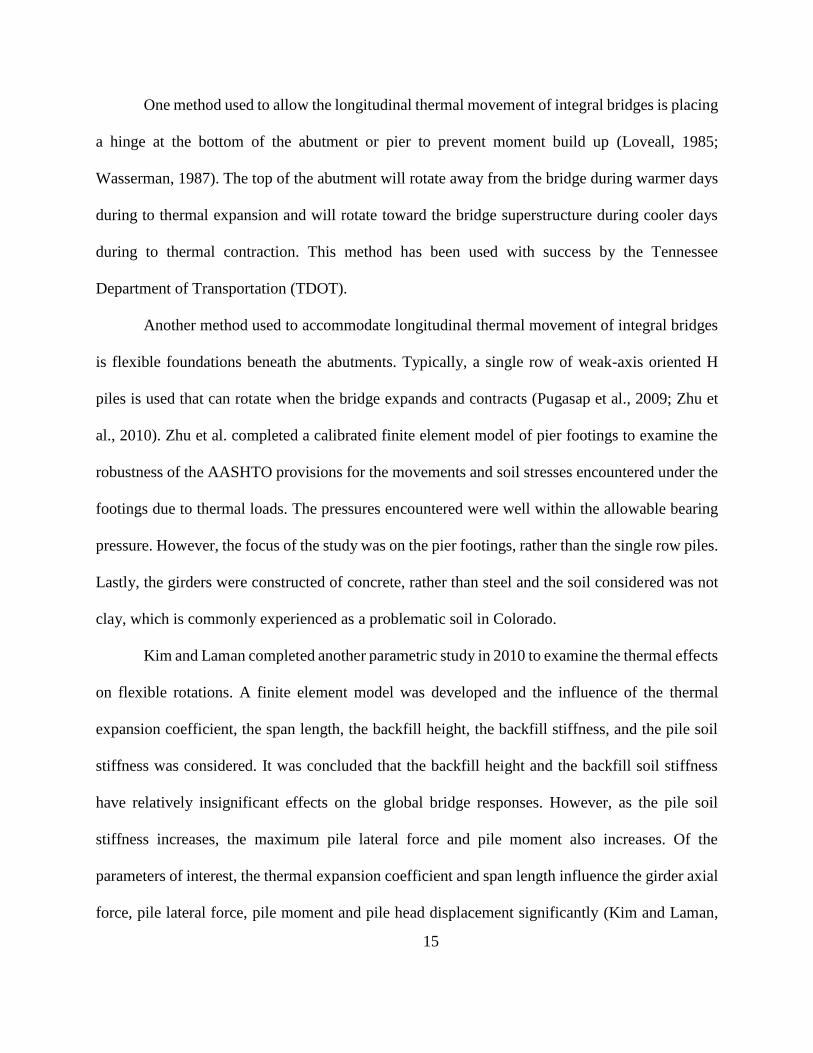
One method used to allow the longitudinal thermal movement of integral bridges is placing
a hinge at the bottom of the abutment or pier to prevent moment build up (Loveall, 1985;
Wasserman, 1987). The top of the abutment will rotate away from the bridge during warmer days
during to thermal expansion and will rotate toward the bridge superstructure during cooler days
during to thermal contraction. This method has been used with success by the Tennessee
Department of Transportation (TDOT).
Another method used to accommodate longitudinal thermal movement of integral bridges
is flexible foundations beneath the abutments. Typically, a single row of weak-axis oriented H
piles is used that can rotate when the bridge expands and contracts (Pugasap et al., 2009; Zhu et
al., 2010). Zhu et al. completed a calibrated finite element model of pier footings to examine the
robustness of the AASHTO provisions for the movements and soil stresses encountered under the
footings due to thermal loads. The pressures encountered were well within the allowable bearing
pressure. However, the focus of the study was on the pier footings, rather than the single row piles.
Lastly, the girders were constructed of concrete, rather than steel and the soil considered was not
clay, which is commonly experienced as a problematic soil in Colorado.
Kim and Laman completed another parametric study in 2010 to examine the thermal effects
on flexible rotations. A finite element model was developed and the influence of the thermal
expansion coefficient, the span length, the backfill height, the backfill stiffness, and the pile soil
stiffness was considered. It was concluded that the backfill height and the backfill soil stiffness
have relatively insignificant effects on the global bridge responses. However, as the pile soil
stiffness increases, the maximum pile lateral force and pile moment also increases. Of the
parameters of interest, the thermal expansion coefficient and span length influence the girder axial
force, pile lateral force, pile moment and pile head displacement significantly (Kim and Laman,

16
2010). Finally, the authors conclude by recommending that the effects of thermal stresses are
included in all integral abutment bridges.
2.7.2 Effects of Bridge Geometry (Skew and Curvature)
Effects of curvature and skew have been examined to determine if global longitudinal
bridge movements can or cannot be totally described by the one-dimensional AASHTO provisions
in cases where the curvature and skew of the bridge are significant. Several transportation agencies
have set limits on the skew and curvature of bridges eligible for integral construction and retrofits
(Burke Jr., 1990; CDOT, 2012; Husain and Bagnariol, 2000). Further understanding of connection
retrofits could help loosen the restraints on skew and curvature limitations. That being said, special
attention should be given to skewed and curved bridges since field observations have confirmed
the high potential for crack development with in long and continuous skewed bridges (this is based
on discussion with Mr. Matt Greer with FHWA).
A three-dimensional finite element model was developed and verified by Moorty and
Roeder (1992) to examine effects of skew, length, width, girder depth, cloud cover, wind speed,
air temperature, bridge temperature differentials, and horizontal curvature in bridges under thermal
loading. Their studies were performed on bridges with bearings between the girder system and the
piers and abutments. Bridges with horizontal curvature were found to exhibit significant radial
displacements near center of curvature and significant tangential displacements at point furthest
away from rigid supports. Also, radial displacements were found to increase as the curvature of
the bridge increased. Lastly, the radial displacements were shown to increase when the stiffness of
bearings were greater (Moorty and Roeder, 1992). This is of importance to integral bridges where
the superstructure connects monolithically with the piers and abutments. The stiffness in these

17
connections is many orders of magnitude greater than the stiffness of a bearing. Therefore, it is not
unreasonable to expect significant stress build up in connections or significant radial movements
in curved bridges without bearing pads that are subjected to thermal expansion and contraction
along their longitudinal axis.
The finite element model developed by Moorty and Roeder also considered the effects of
skew. The longitudinal and transverse deflections due to thermal loads were found to vary in the
transverse direction in skewed bridges. Displacements were greatest at points furthest away from
rigid supports. Lastly, it was recommended that bearings used on skewed bridges be unguided (not
restricted to a single line of movement) to allow for transverse movements (Moorty and Roeder,
1992). In an integral bridge without bearings, however, these movements would be restrained, and
the bridge would need to be able to accommodate these stresses through movement in a different
location or with the strength of structural elements.
Questions remain about the effects of curvature and skew in integral bridges. However,
understanding the movement of non-integral bridges provides a link to how the stresses would
accumulate in curved and skewed integral bridges. Current AASHTO commentary (Section
C3.12.2.1) states that bridges with large skew or curvature should not be built upon bearings that
only allow movement in the longitudinal direction due to radial or tangential movement that is
expected. Understanding of restraints and connections used combined with structural solid
mechanics could yield estimate for the accumulated stresses. Or, the vertical supports could be
decreased in stiffness to allow for the thermal movements to occur without the accumulation of
stress.

18
2.7.3 Potential Increase in Moment Capacity
Eliminating deck joints and making the girders and deck continuous has the potential to
increase moment capacity. However, due to the multiple ways a bridge can be connected and made
continuous, the extent of the increased load rating is largely dependent on which detail is used and
what elements of the superstructure become connected (Tsiatas and Boardman, 2002). A study
conducted in 2002 by Tsiatas and Boardman examined Deck Only, Deck and Top Flange, Deck
and Bottom Flange, Deck, Top and Bottom Flange, and Full Moment Splice connections. The
study concluded that no increase in moment capacity was exhibited when Deck Only and Deck
and Top Flange connections were used. The Deck Only and Deck and Top Flange connections
also were found to possess the highest potential for cracking due to the negative moment
experienced in the bridge over the piers or supports.
Connections that did improve the moment capacity of the bridge included the Deck, Top
and Bottom Flange connection and the Full Moment Splice connection (Tsiatas and Boardman,
2002). Unsurprisingly, these connections are more expensive and laborious to construct. However,
for bridges that are expected to carry more traffic in the near future, this option may be worth
considering. Worth noting is that the model used to draw these conclusions was two-dimensional.
It is uncertain whether this model included some of the benefits or disadvantages of the local
behavior of the connection types considered. A three-dimensional model and more field
verification of this model would strengthen the claims asserted.
2.8 Local Superstructure Behavior
The parameters and areas of interest of local behavior for bridges with deck joints differ
from those without. Local superstructure behavior of interest for bridges with deck joints includes

19
corrosion of girders under leaking joints, joints unable to perform due to debris build up and
performance of joints and bearing pads under extreme temperatures. Local superstructure behavior
of interest for integral bridge construction and retrofits (bridges without deck joints) includes
lateral-torsional buckling (LTB) risk, thermal stress differentials in the superstructure cross-
section, stresses in connections, rotation at girder ends, shear lag at girder ends, and understanding
the advantages and disadvantages of numerous connection types. Local behavior of these forms
could be non-linear and not fully described by two-dimensional models. Instead, verified, detailed
three-dimensional finite element analysis would increase the understanding of the complex
behaviors exhibited. An examination of previous research completed in these areas of interest
follows.
2.8.1 Corrosion
Corrosion, one of the central issues with deck joints, is caused in the superstructure when
deck joints leak (Hawk, 2003; Lam et al., 2008). This corrosion at the deck joints, which are
commonly located at the piers, abutments, or other vertical supports, causes the structural integrity
of the superstructure and bearings to deteriorate. Often, local behavior of the bearings, connections,
girders, pier caps, and piers under these decks will be adversely affected. The use of deicing
chemicals, and their subsequent runoff from roadways, increases the rate of corrosion to girder
systems under deck joints (Tsiatas and Boardman, 2002). When deck joints leak, maintenance and
eventually replacement are necessary to maintain a safe structure. Various bridges in the state of
Colorado have suffered from similar deterioration. The Colorado Bridge Enterprise (CBE) has
been formed in 2009 with the purpose of providing funding to repair, reconstruct and replace
bridges designated as structurally deficient or functionally obsolete, and rated poor. A list of

20
bridges that fall under these conditions can be fond in the CBE list at
https://www.codot.gov/programs/BridgeEnterprise/documents/faster-statewide-bridges.
2.8.2 Blocked Expansion
In order to function properly, expansion joints must be able to freely expand and contract
without significantly affecting the driving surface of the road. As illustrated in Figure 2-2, debris
build up in an expansion joint less than six months old can prevent it from closing in warmer
weather to accommodate thermal loads (Chen, 2008). Routine maintenance is required to keep
expansion joints in working order.
Figure 2-2. Debris in expansion joint in service for less than six months (Chen,
2008)

21
If excessive debris is allowed to build up in an expansion joint, pavement growth can occur.
Pavement growth (PG), as defined by the Michigan Department of Transportation (MDOT), is the
widening of joints from debris build up. Another major cause of PG is from concrete pavement
that expands over time, causing joints to close. This phenomenon has been observed in bridges on
I225 and I 25 in Colorado and has been successfully addressed with pavement relief joints.
If traffic removes a compression seal or debris builds up from other causes, the effect on
the structure can be severe. When a joint with debris build-up opens further due to reduction of
average bridge temperature, the debris settles further into the joint and now takes up the entire new
width of the joint opening. This is very damaging because at this point, the joint will not be able
to close any further than the current cool weather, wider debris opening. As a result of this
increased opening, more debris is allowed to build up and the distance from one end of the
pavement to the other “grows”. If the average bridge temperature were to increase, the joint would
not be able to close to alleviate thermal stresses. However, if the temperature only decreases to a
greater extent, the joint will open further, and the newly added debris will settle into the joint and
prevent even more movement, as shown in Figure 2-3. This cycle continues if the bridge deck joint
is not maintained and significant stresses can be induced into the bridge local connections, bearing
pads, and superstructure elements (Rogers et al., 2012). Eliminating deck joints would allow for
reduction of damage or reduction of cost of maintenance to prevent damage.

22
Figure 2-3. Cycles of Pavement Growth (Rogers and Schiefer, 2012)
2.8.3 Lateral Torsional Buckling Risk for Steel Girders
In bridges that are constructed without deck joints originally or retrofitted such that deck
joints are eliminated, a potential lateral-torsional buckling risk occurs in composite steel girder
systems. Positive moment regions of the bridge (near mid-span) exhibit compressive stresses on
the top of the superstructure cross-section. Since most steel girder systems are composite with a
concrete deck, the neutral axis of the cross-section is raised, and the majority of the compressive
stresses are carried in the concrete deck in the positive moment regions of the bridge. The
compression that occurs in the top flange is relatively small and the flange is held in place by a

23
composite concrete deck. However, in the negative moment regions of the bridge, which are
commonly where a deck joint is eliminated and the bridge can be made continuous, the new cross-
section under negative moment will exhibit compressive stresses on the bottom flange of steel
girders that is not supported or carried by a composite concrete deck (Vasseghi, 2013). These high
compressive stresses in the bottom of the section below the neutral axis and the tensile forces
experienced above the neutral axis cause a potential for lateral-torsional buckling or kicking-out-
of-plane. Analysis of this type of behavior is requisite to making a superstructure continuous and
stable.
Compact steel sections are cross-sections that are not at risk of lateral-torsional buckling.
Whether or not standardly compact sections, as specified by AISC Code are clear of this risk in all
integral bridges could be verified by numerical modeling or laboratory tests. Sections that are not
classified by the American Institute of Steel Construction as compact should definitely be analyzed
for this behavior before a retrofit or new construction of an integral steel bridge is completed. The
stresses occurring in the connections and girder system are a function of what kind of connection
and girders are in place. Therefore, an analysis of buckling behavior for current and possible
retrofit connections and girder systems would be a helpful step in quelling the potential for lateral-
torsional buckling. Lateral bracing in the form of stiffeners or torsional bracing in the form of
diaphragms or cross frames can be implemented near the part of the girder in compression to
prevent lateral torsional buckling (Vasseghi, 2013; Segui, 2012).
2.8.4 Temperature Gradient
Another significant factor to consider when eliminating deck joints is uneven temperature
in the transverse and vertical direction across a bridge and girder cross-section. During times of

24
the day in which the ambient air temperature is changing, the entire bridge is also changing in
temperature through radiation, convection, and conduction. This could cause deck cracking, which
has been observed in Colorado Bridges, as a result of continuity. Undoubtedly, the mix designs
and placement are other contributors to deck cracking. Radiation is the energy emitted by the sun
in the form of electromagnetic waves through the medium of the atmosphere. Usually, only the
deck receives direct solar radiation, while the girder system does not. Convection is the mode of
heat transfer between the bridge’s solid surface and the adjacent air that is in motion (e.g. wind)
and involves the combined effects of fluid motion and conduction. The outer girders and deck may
experience the effects of convection to a greater extent than the interior girders. Conduction is the
transfer of energy of more energetic particles in one solid to less energetic particles in another solid
through direct contact (Cengel, 2012). The constant and inconsistent temperature changes across
the cross-section manifest themselves in uneven expansion, or, if restrained, uneven thermal
stresses in the bridge structure.
In 2008, Li et al. completed a study on the thermal loading and expansion joint movement
of Confederation Bridge, an existing, long-span concrete girder bridge. Though this is not a steel
bridge, the methodology to analyze and monitor a concrete bridge would be similar for a steel
bridge. Temperature differentials in the vertical and transverse direction in the girder cross-section
were examined with three years of data gathered from thermocouples installed on the bridge. The
rate of temperature change and temperature gradient was discovered to develop in different rates
and patterns in the transverse direction than in the vertical directions (Li et al., 2008). It was also
found that shallow sections did not need to consider temperature variation in the transverse
direction (the direction perpendicular to traffic flow). Though this seems like a promising way to
simplify a design method, what constitutes a shallow section was not explicitly stated by the

25
authors. Rather, the shallowest section of the bridge, a concrete box girder with a height of 177 in
(4.5 m) was the shallowest section considered and it did not appear to have significant temperature
variation in the transverse direction (Li et al., 2008). A boundary between shallow sections and
deep sections is never explained, but a qualitative conclusion that shallow sections have negligible
temperature variation in the transverse directions helps further understanding about thermal effects
in a cross-section. However, a quantitative definition of shallow in relation to other parameters
would be more useful to a practitioner designing an integral bridge.
Another notable study was performed by French et al. in 2013 to assess the thermal gradient
effects in the Interstate 35 St. Anthony Falls Bridge in Minneapolis, MN. This posttensioned
concrete box girder bridge was monitored over a duration of three years. Finite element modeling
in ABAQUS was developed and gradients from two code provisions were considered. Vertical
thermal gradients from AASHTO LRFD Bridge Design Specifications developed by Imbsen et al.
(1985) and the New Zealand Bridge design code developed by Priestley (1978) were considered.
A fifth-order design thermal gradient, as specified by the New Zealand Bridge Design Code, was
determined to be the most appropriate for this bridge with the top surface temperature matching
the temperature assigned in the AASHTO provisions for Minneapolis, MN (French et al., 2013).
Additionally, the global structural demand modeled with the AASHTO provisions of vertical
thermal gradient were found to be much lower than the measured stresses (French et al., 2013).
This study further encourages the examination of the vertical gradient developed by Imbsen et al.
(1985) in AASHTO for other bridge girder types and in other geographical locations.
Further studies performed by Chen (2008) were conducted to analyze temperature
differentials and the corresponding thermal stresses in steel bridges in Texas. This study is
particularly relevant because the bulk of research involving elimination of deck joints and thermal

26
gradients has been conducted on concrete girder bridges. Analysis in this study involved finite
element models verified by field monitoring and experimental testing performed in the Ferguson
Structural Engineering Laboratory in Austin, Texas. The dissertation addresses the robustness of
thermal stresses that occur in bridges that are accounted for in the current AASHTO Bridge Design
Specifications. Also, stresses that are not currently accounted for in the AASHTO Bridge Design
Specifications are examined (Chen, 2008). According the temperature contour map provided by
AASHTO the temperatures range is cooler in Colorado than in Texas. The maximum expected
temperature for Colorado and Texas is 100oF-110oF and 105oF-115oF, respectively. The minimum
expected temperature in Colorado and Texas is approximately -30oF - 0oF and 10oF - 40oF,
respectively (AASHTO, 2012, Figure 3.12.2.2-1 and Figure 3.12.2.2-2). The range of expected
temperatures for Colorado is larger than in Texas and therefore the stresses found in steel bridges
in Texas may actually be less than what a similar steel bridge in Colorado would experience.
Though current AASHTO provisions only require consideration of the total longitudinal
thermal movement based on the average bridge temperature, stresses due to temperature
differentials in the cross section were shown to commonly be above +/- 5 ksi (34.5 MPa) in steel
box girder bridges in Texas. Though different girder widths, depth and bridge location would
change the value of these stresses, it is clear that the significance of these stresses is worth
analyzing in Colorado’s steel bridges if an order of magnitude of 5 ksi (34.5 MPa) is reached on a
regular basis in Texas steel bridges.
The heating and cooling of steel girder systems with composite bridge decks was analyzed
in Chen’s research. Due to the differences in thermal expansion coefficient and different exposure
to radiation, convection and conduction, the heating and cooling of a composite girder cross-
section is non-uniform as shown in Figure 2-4 and 2-5. If these two components of the

27
superstructure, the deck and the girder, are restrained in the same place, thermal stresses will
develop due to the uneven heating or cooling of the structure. Accounting for these additional
stresses through increases in material strength, flexible piles, hinged abutments, and/or bearings
could help alleviate stresses in this local behavior.
Figure 2-4. Vertical Temperature Distributions of Heating of Steel Composite
Girders (Chen, 2008)
Figure 2-5. Vertical Temperature Distributions of Cooling of Steel Composite
Girders (Chen, 2008)
Regarding integral bridges, material strength must be increased, or movement must be
allowed to accommodate these uneven movements to occur. Non-integral bridges with expansion

28
joints can expand or contract at slightly different rates without inducing stresses because of the
gap that is present. For example, if the concrete deck heats and expands sooner and then the steel
girder below it due to solar radiation on the deck, the gap in the expansion joint would close more
near its top and less near its bottom. However, this uneven expansion joint opening would induce
no stresses. For integral bridges, on the other hand, any uneven thermal expansion or contraction
would induce a stress in the element because it is not allowed to move independently from the
adjacent span at the vertical supports. Movements would need to be absorbed through pier
deflection, foundation deflection, strength of material, bearing movements, girder deformation, or
a combination of all of these (Chen, 2008). It should be noted that for both integral and non-integral
bridges, stresses at the interface of the steel girders and concrete deck would be expected due to
the uneven heating shown in Figure 2-4 and 2-5. The magnitude of these stresses is relatively
unexamined, but worth analyzing for design of shear studs and connections between the deck and
the girder system.
Effort also was made in this study to identify the conditions with the greatest thermal
effects. It was found that bridges with north-south orientation, shorter lengths of the concrete deck
overhang, deeper steel girder webs, thinner concrete decks, and wider girder spacing resulted in
the most extreme cases of thermal stresses (Chen, 2008). Though this is a qualitative result, it may
be beneficial to know these most extreme conditions to strategize a way to reduce thermal effects
in the design of a new bridge.
2.8.5 Temperature Data
Lastly, a statistical analysis was performed to compare the temperature data found with the
expected values provided in the AASHTO Bridge Design Specifications. The temperatures
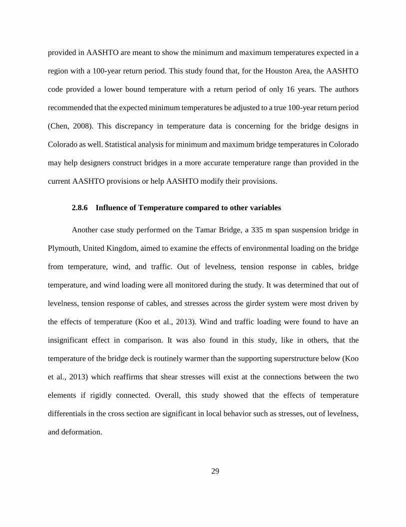
29
provided in AASHTO are meant to show the minimum and maximum temperatures expected in a
region with a 100-year return period. This study found that, for the Houston Area, the AASHTO
code provided a lower bound temperature with a return period of only 16 years. The authors
recommended that the expected minimum temperatures be adjusted to a true 100-year return period
(Chen, 2008). This discrepancy in temperature data is concerning for the bridge designs in
Colorado as well. Statistical analysis for minimum and maximum bridge temperatures in Colorado
may help designers construct bridges in a more accurate temperature range than provided in the
current AASHTO provisions or help AASHTO modify their provisions.
2.8.6 Influence of Temperature compared to other variables
Another case study performed on the Tamar Bridge, a 335 m span suspension bridge in
Plymouth, United Kingdom, aimed to examine the effects of environmental loading on the bridge
from temperature, wind, and traffic. Out of levelness, tension response in cables, bridge
temperature, and wind loading were all monitored during the study. It was determined that out of
levelness, tension response of cables, and stresses across the girder system were most driven by
the effects of temperature (Koo et al., 2013). Wind and traffic loading were found to have an
insignificant effect in comparison. It was also found in this study, like in others, that the
temperature of the bridge deck is routinely warmer than the supporting superstructure below (Koo
et al., 2013) which reaffirms that shear stresses will exist at the connections between the two
elements if rigidly connected. Overall, this study showed that the effects of temperature
differentials in the cross section are significant in local behavior such as stresses, out of levelness,
and deformation.

30
2.9 LCCA Process
LCCA involves determining all costs associated with a piece of infrastructure over its
design life. These costs range from design and construction to maintenance and user costs to
environmental and vulnerability costs (Frangopol and Liu, 2007; Marques Lima and de Brito, 2010;
Hawk, 2003; Safi et al., 2015; Kim et al., 2010; Hatami and Morcous, 2014; Reigle and Zaniewski,
2002). Once all costs have been identified, they are referenced to a point in time and the total
calculated. This total cost for an infrastructure’s entire life-span is the LCC which can then be
compared to the life-cycle cost of other designs for the same piece of infrastructure. LCCA
becomes an effective way to compare designs and support the choice of a particular design as the
most economically effective choice overall even if its initial cost is high (Hatami and Morcous,
2014). This can be particularly helpful when talking to the public or working in public design and
construction (Al-Wazeer et al., 2005).
Like any analysis process, LCCA is based on a couple of assumptions. Performing an
LCCA assumes that there are multiple designs for the same desired piece of infrastructure, whether
bridge, building, or roadway, and that each of these designs can meet the needs and required
performance capabilities. Additionally, it is assumed that each of these designs has varying initial,
operating, and maintenance costs and can have varying lengths of life-span (University, 2005).
Therefore, these assumptions must be true and taken into consideration when performing a LCCA.
If the case of several designs having different life-spans is the case, they must be manipulated to
have a common life-cycle to compare them using a LCCA. For example, if design A has a life-
span of 25 years and design B has a life-span of 50 years, then an analysis could assume that at the
end of design A's life span a second design A is built to have a life-span of 50 years’ total. Then
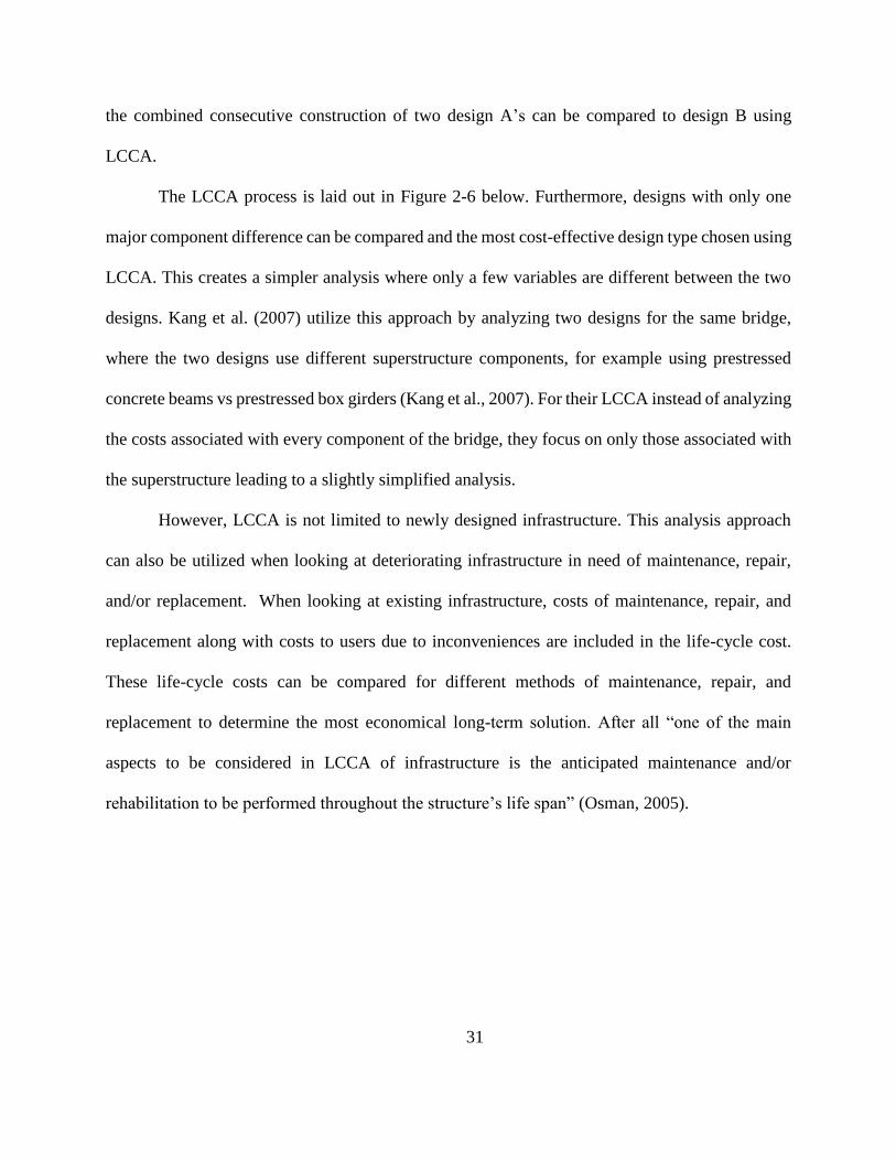
31
the combined consecutive construction of two design A’s can be compared to design B using
LCCA.
The LCCA process is laid out in Figure 2-6 below. Furthermore, designs with only one
major component difference can be compared and the most cost-effective design type chosen using
LCCA. This creates a simpler analysis where only a few variables are different between the two
designs. Kang et al. (2007) utilize this approach by analyzing two designs for the same bridge,
where the two designs use different superstructure components, for example using prestressed
concrete beams vs prestressed box girders (Kang et al., 2007). For their LCCA instead of analyzing
the costs associated with every component of the bridge, they focus on only those associated with
the superstructure leading to a slightly simplified analysis.
However, LCCA is not limited to newly designed infrastructure. This analysis approach
can also be utilized when looking at deteriorating infrastructure in need of maintenance, repair,
and/or replacement. When looking at existing infrastructure, costs of maintenance, repair, and
replacement along with costs to users due to inconveniences are included in the life-cycle cost.
These life-cycle costs can be compared for different methods of maintenance, repair, and
replacement to determine the most economical long-term solution. After all “one of the main
aspects to be considered in LCCA of infrastructure is the anticipated maintenance and/or
rehabilitation to be performed throughout the structure’s life span” (Osman, 2005).

32
Furthermore, there is more extensive application of LCCA to existing structures and
relatively little application to new structures (Safi et al., 2015). This is despite the fact that LCCA
applied to any structure will produce long term savings, and if applied to a new structure it will
Figure 2-6 Life-Cycle Cost Analysis Process Flow Chart
Life-Cycle Cost Analysis (LCCA)
Collect all designs to analyze
Collect Costs
for each
project
Calculate the Total Life-Cycle Cost (LCC) for each Design
Select Design with lowest LCC for project
Determine Costs to be Considered

33
produce the maximum savings because they were applied over the entire length of the structure’s
lifetime (Agency and Severn, 2000). However, an existing structure can also benefit from LCCA
due to the structural system being composed of many smaller parts and each of these has a different
and likely shorter lifespan than the overall system. Furthermore, these components are not usually
easy or simple to replace and therefore the costs associated with that replacement or repair can be
critical (Riedel et al., 1998). This is not to say that designing a structure with these costs in mind
at the beginning with an LCCA is not better in the long run, it is, however, using LCCA in the
continued maintenance is also beneficial.
There are several aspects that hinder the application of LCCA to new structures. One that
is proposed by Safi, et. al. that could be hindering the application of LCCA to new bridges in
particular is the assumption that bridge management systems (BMSs) are completely separate from
LCCA, when in reality much of the data used in BMS could help determine an accurate LCCA
(Safi et al., 2015). Another problem could simply be an incomplete understanding of LCCA
benefits among implementers (Goh and Yang, 2014). Additionally, LCCA requires foresight, the
funds to support a slightly more expensive design with long term savings in mind, and time to
perform the analysis. These deterrents are slowly becoming overwhelmed by the benefits of LCCA
as they become better known and supported by federal agencies.
As the benefits of using LCCA in infrastructure analysis become common knowledge, it is
suspected that more and more states will implement it as a regular practice. Utilizing LCCA can
enable government and state agencies to make the most economical design and repair decisions
regarding public infrastructure over the infrastructure’s entire life-span. This can lead to minimized
maintenance, repair, and replacement costs as well as minimize delays and costs to users over the
structure’s life-time.

34
All infrastructure is an investment; public infrastructure is an investment of the public's
funds consequently, interest in the best use of funds for infrastructure maintenance is growing.
According to Goh and Yang, before 1990 there was very little attention given to LCCA, however
in 1990 the Federal Highway Administration began to encourage its use in projects and later made
it mandatory for projects of $25 million or more (Goh and Yang, 2014). Research and application
have been increasing in all areas of infrastructure since this mandate. LCCA is becoming an
integral part of design and maintenance of infrastructure and therefore should not be taken lightly.
2.10 Components of LCCA
Several components make up the costs analyzed in a LCCA. These components can mean
slightly different things for different types of infrastructure, for example bridges versus buildings
will have slightly different costs associated with them. Common cost components include:
initial/construction, operation, maintenance, renewal/replacement, cost of capital, and user
(Board, 1998). Below, in Figure 2-7 is a flow chart showing the components of each cost,
followed by a general description of each of the main components of cost that are related to
LCCAs.
Initial Cost is perhaps the simplest component of LCCA cost components. The initial cost
is what the project will cost up front. This includes the costs of the design, the contract, the
project management, the construction, and the final inspection and certification, if necessary.

35
Life-Cycle Cost Analysis
(LCCA)
Operation
Cost
Maintena
nce Cost
Cost of
Capital
Initial/
Constructi
on Costs
User Cost
Replacemen
t/Renewal
Cost
Design
Contract
Project
Management
Construction
Final Inspection
Employees
Machinery
Power/
Electricity
Regular
Inspections
Weather
Proofing
Cleaning/
Painting
Required
Updating
Renewing of
Systems/
Applications
Replacement of
Individual Parts
Replacement of
Whole Structure
Money’s Time Value to
Owner Investor
Taxpayers
Local Residents
Drivers/
Commuters
Employees
Emergency
Personnel
Figure 2-7 Life-Cycle Cost Analysis Costs Flow Chart

36
Initial cost is what has been traditionally used to choose which design to use for a
project, independent of any of the other costs. The agency would traditionally receive
several design bids and would choose the lowest bid (Safi et al., 2015). The lowest bid
procurement process does not account for any of the other cost components occurring
throughout the structure’s life. Instead of choosing the project with the lowest initial bid,
the design could be chosen based on lowest LCC bid, which is what is proposed to the
European Union Directive by Safi et al. ( 2015).
Operation Cost is the cost needed to operate the infrastructure over its life-span.
This cost varies greatly depending on the infrastructure being analyzed. Some structures
will have little to no operational costs, such as a simple bridge. However, other structures,
such as buildings, drawbridges, or toll roads will have various operation costs associated
with employees and machinery. These costs could include employees to run the machinery
or toll booths and electricity to power the structure.
Maintenance Cost is the cost of maintaining the infrastructure in a safe, usable, and
functional condition. Maintenance costs can include regular inspections, weather proofing,
cleaning, painting, and any type of required updating. Depending on the structure these
maintenance costs could be as frequent as monthly or as infrequent as every few years. The
importance of having funds to perform the maintenance is also going to depend on the
structure. For example, the repainting of a steel bridge to prevent corrosion could have
more importance than the repainting of a concrete building on schedule because the steel
bridge is typically going to be more immediately susceptible to deterioration than the
building.

37
Renewal/Replacement Costs depend on the object of analysis, whether the
objective is renewal of the structure or replacement of the structure in part or entirety.
Renewal costs would be applicable to costs due to the renewing of software or electric
systems. Whereas a replacement cost would apply to the replacement of anything
connected to that piece of infrastructure or equipment. This could range from the
replacement of a single element to the entire structure.
Cost of Capital is the money's time value to the owner, investor, or in the case of
public works the taxpayers (Board, 1998). This cost adjusts for the fact that choosing a
design using LCCA often means a higher initial cost compared to designs that do not use
LCCA and would have higher maintenance and repair costs later. Therefore, the money's
time value is accounting for using that extra money to have a lower overall cost instead of
using it to invest in something else.
User Cost includes any costs to users of the infrastructure or system. This can
include costs to drivers and passengers due to construction or traffic blocks for repair or
replacement (“Life Cycle Cost Optimisation in Highway Concrete Bridges Management,”
n.d.). Another example of user costs could be due to relocating of employees in the case of
a building's repair or maintenance.
2.11 Components and Parameters Related to Bridge Maintenance
Bridge design, maintenance, repair, and replacement have specific costs within each
general cost component of LCCA. Below Figure 2-8 shows a flow chart for the LCCA
costs specific to bridges. In order to compose a thorough LCCA for a bridge, each

38
component of the LCCA must include all aspects that affect the bridge. In other words, the
parameters must be tailored to the infrastructure and its environment, in this case a bridge
and the outdoors (Hawk, 2003).
There are also parameters in addition to the cost components that need to be taken
into consideration and are of particular interest to bridges. These include the service life of
the bridge and the analysis period of the LCCA. The service life is the time period over
which the components of the bridge and the bridge itself are in serviceable condition based
on the industry standard for acceptable condition limits. The service life does not always
equal the design life, a design life might account for repair or replacement of some bridge’s
substructure parts. However typical Best Management Practices (BMPs) assume a service
life between 70 and 100 years. On the other hand, the analysis period is the period of time
over which all costs in the LCCA are analyzed and brought to a total present value. This
time period can be shorter or equal to the service life of the bridge, depending on the period
the buyer wishes to analyze based on what years are of most importance. Nonetheless,
typically the analysis period is made equal to the service life in order to simplify the LCCA
process (Hawk, 2003). However, if the analysis period is less than the service life there is
a value left due to the remaining serviceable life of the bridge.
Initial and construction costs are some of the simplest components of a LCCA for
bridges. Both are constant values, with little uncertainty associated with them because they
are onetime costs at the beginning of the bridge’s life. The initial cost is composed of the
design and contractor costs, while the construction cost is the cost of the construction
materials, workers, and time, as well as any road closure costs due to the bridge’s

39
construction. This last aspect of construction cost affects user costs as a road or lane
closure and/or detour will affect the drivers in the area.

40
Life-Cycle Costa
Analysis
(LCCA)
For Bridges
Operation
Cost
Maintena
nce Cost
Initial/
Constructi
on Costs
User Cost
Replacement
Cost
Design
Contractor/
Contract
Project
Mangment
Construction
Final Inspection
Employees
Machinery
Power/
Electricity
Regular
Inspections
Weather
Proofing
Cleaning/
Painting
Required
Updating
Repair of small
components
Replacement of
components in
part of whole
Replacement of
Whole Structure
Local Residents
Drivers/
Commuters’
delay
Employees
Emergency
Personnel
Building
Materials
Worker
s,
Traffic
Control
, Time,
Materi
als
Toll
booths,
Draw
bridge,
Presence of
Expansion
Joints?
Traffic
Load,
Type of
Materi
al,
Locatio
n
Vehicle
Operation/
Idling
Accidents
Salvage
Cost
Value of
Remaining
Service Life
Figure 2-8 Life-Cycle Cost Analysis Costs Flow Chart for Bridges

41
The maintenance costs for bridges depend on several key factors. The planned life-span, the
bridge structural material (i.e. steel or concrete), the anticipated traffic load, the environment,
whether or not preventative maintenance is included (Reigle and Zaniewski, 2002) all affect
maintenance. Additionally, whether or not the bridge contains an expansion joint (and if it does, the
type of expansion joint used) can also impact the maintenance costs. In fact, when considering the
LCCA of a bridge with expansion joints, they “should be considered a critical factor” (Savioz, 2014).
Expansion joints are very susceptible to clogging, corrosion, and deterioration due to dynamic load
impacts on their various components, which are more delicate when compared to a steel or concrete
girder. Consequently, the probability of maintenance needed on the bridge will increase with the
presence of an expansion joint. Furthermore, because they are a weaker bridge component that spans
the width of the bridge, they can have significant impacts on other costs such as user and replacement
costs as well.
Repair and/or replacement costs for bridges are composed of the cost of repairing and/or
replacing each component of the bridge with respect to that component’s life-span in comparison to
the overall bridge’s desired life-span.
User Costs for a bridge are composed of costs to the drivers and residents who were affected
by the closing of or limiting of traffic on the bridge due to maintenance, repair, or replacement. They
are in some ways the most involved costs in an LCCA because they involve the public which
increased variability. These costs are due to delays to drivers personally, costs of vehicles idling in
traffic, and accident rate increases due to road work (Kim et al., 2010; Reigle and Zaniewski, 2002).
As such they should be minimized by minimizing the disruption caused by the repair or maintenance
(Agency and Severn 2000). This could be done by limiting the closure to one lane at a time and
performing maintenance, repair, or replacement in stages/portions. These aspects can be categorized
as three individual costs the sum of which equals the User costs included in a LCCA. Kim et al.

42
(2010) define these costs and formulate the following equations to use in a LCCA. The driver delay
cost, vehicle operating costs, and accident costs are defined in equation form below and all variables
are listed in Table 2-1 (Kim et al., 2010).
Driver Delay Cost = (𝐿
𝑆𝑎−
𝐿
𝑆𝑛) × 𝐴𝐷𝑇 × 𝑁 × 𝑤 (2.1)
Vehicle Operating Cost = (𝐿
𝑆𝑎−
𝐿
𝑆𝑛) × 𝐴𝐷𝑇 × 𝑁 × 𝑟 (2.2)
Accident Cost = 𝐿 × 𝐴𝐷𝑇 × 𝑁 × (𝐴𝑎 × 𝐴𝑛) × 𝑐𝑎 (2.3)
Table 2-1 Parameters Assumed for User Cost Computation (Kim et al., 2010)
Parameters Symbols
Length of Affected Roadway (km) L
Average Daily Traffic (ADT) ADT
Normal Driving Speed (kmph) Sn
Roadwork Driving Speed (kmph) Sa
Normal Accident Rate (per million vehicles) An
Roadwork Accident Rate (per million vehicles) Aa
Hourly Driver Cost (US$) w
Hourly Vehicle Operating Cost (US$) r
Cost per Accident (US$) ca
Required Days for Repair Nrepair
Required Days for Replacement Nreplace
Each of the parameters in Table 2-1are used in the three user cost equations (2.1), (2.2), and
(2.3). Furthermore, each is specific to that bridge. Therefore, the parameters in Table 2-1 above are
an example of parameters that might be used for a LCCA and would need to be adjusted for a
different specific bridge based on its location, current rates, expect traffic, dimensions, and any other
available information.
2.12 Maintenance of Bridges with Expansion Joints
The maintenance, repair, and replacement (MR&R) procedures and the costs associated with
them for bridges are critical to a bridge’s LCCA. The MR&R are a substantial portion of the total

43
LCC for a given bridge (Mao and Huang, 2015). They can be divided up as MR&R costs for each
component of the bridge, such as the beams, columns, deck, and expansion joints (Kang et al., 2007).
In fact in 2002 a study showed that 20-50% of total infrastructure costs were due to MR&R in various
countries (Mao and Huang, 2015). Therefore, the cost of MR&R is directly related and important to
the overall LCCA. The many factors that influence MR&R costs for bridges are summarized in
Figure 2-9 below. Traditionally LCCA in general and MR&R costs specifically have been analyzed
using statistical models and analysis, such as simple regression and overall trends to calculate costs
based on collected data (Mao and Huang, 2015). Furthermore, many traditional LCCA methods also
neglect user costs and preventative maintenance benefits and costs due to a lack of data or the
complexity of the calculations which can affect all costs including MR&R costs (Reigle and
Zaniewski, 2002).
Most LCCA models do not give a specific approach for the maintenance costs which can
make it hard to determine that cost (Mao and Huang, 2015; Hawk, 2003). A more accurate and
specific method would be to include probabilistic approaches, because “estimation depends on
predicting how bridges deteriorate over time and what subsequent actions are taken” (Mao and
Huang, 2015). These costs should then be based on those predictions. Mao and Huang (2015)
conducted a study to estimate the MR&R costs of a bridge using a Monte Carlo simulation applying
probability distributions. They chose an expansion joint as their example bridge component,
nonetheless the analysis could be applied to any bridge component and then the sum of all MR&R
costs for each component would equal the total MR&R costs for the bridge.

44
Figure 2-9 Factors affecting MR&R Costs for Bridges
However, using just a stochastic model utilizing probability of deterioration or defect and the
probability that further deterioration will develop has limitations too. For example, using a strict
Markovian probability model might not account for unique factors affecting the current state of the
bridge. The probability of transition from one form of deterioration to another requires sufficient
observed data related to the specific bridge which may not be available, especially for newer bridges
(Mao and Huang, 2015). Furthermore, Huang and Mao argue that the future condition of the bridge
is affected by the bridge’s history, while Markov processes are in part defined by the fact that future
conditions only depend on the current condition. While, probability should be a key part of predicting
defects and deterioration and thus MR&R costs, it should not be the sole source of that information,
other current and historical observations and the overarching deterioration processes should be used
to enhance that prediction.
MR&R Costs
for Bridges
Girders
Columns Slab
Expansion
Joints
CablesMachinery
Piers
Regular
Inspections
Regular &
Preventative
Maintenance
Regular
Repairs
Environment
Traffic
Load
Historical Data
Types of Bridge
Components
Probability of
Deterioration Age/
Design Life

45
Typically, bridges are inspected visually for signs of deterioration and/or defects. While
visual inspection can be subjective depending on the person, the bridge, and the governing guidelines
or procedures, it still provides data for each aspect of a bridge. Furthermore, because bridges have
been regularly visually inspected for the past forty years in the US and for many years in other
countries as well, there is a wealth of data and knowledge that if made available could be used as a
basis for a deterioration model prediction and the evaluation of MR&R costs (Mao and Huang, 2015).
These observations and archived data could be used to compliment a probability matrix in order to
predict the future needs for MR&R of a bridge.
Furthermore, expansion joints are common in various forms in most bridges and are therefore
a key, and at times critical, component for maintenance of a bridge, as well as a main component
affecting costs in an LCCA. While most manufacturers will tout their expansion joints as having long
service lives free of maintenance, in the field this is seldom true. In fact the joints are commonly the
first bridge components to need maintenance or repair (Lima and de Brito, 2010). This is due to
their experiencing millions of impact loads from vehicle wheels throughout their lifetime. These
repeated impact loads can result in failure due to fatigue cracking (Savioz, 2014). Their deterioration
can also be increased if water and/or debris is able to creep into the joint. Therefore, choosing the
best type of expansion joint for the bridge and environment is critical to minimizing maintenance
and replacement costs.
While joints are not an expensive part of the initial cost of a bridge, usually only about 1%
of the total construction cost (Lima and de Brito, 2010), as discussed above they can have a
disproportionate effect on the maintenance/replacement costs over the life span of the bridge. A study
in Portugal showed that over “the previous 3 years, more than 20% of the bridge conservation costs
were related [to] the repair and replacement of expansion joints” ( Lima and de Brito, 2010).
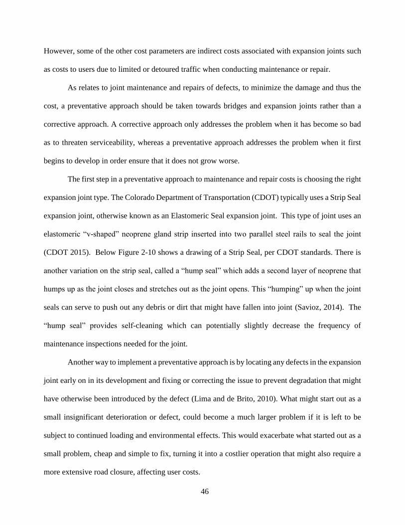
46
However, some of the other cost parameters are indirect costs associated with expansion joints such
as costs to users due to limited or detoured traffic when conducting maintenance or repair.
As relates to joint maintenance and repairs of defects, to minimize the damage and thus the
cost, a preventative approach should be taken towards bridges and expansion joints rather than a
corrective approach. A corrective approach only addresses the problem when it has become so bad
as to threaten serviceability, whereas a preventative approach addresses the problem when it first
begins to develop in order ensure that it does not grow worse.
The first step in a preventative approach to maintenance and repair costs is choosing the right
expansion joint type. The Colorado Department of Transportation (CDOT) typically uses a Strip Seal
expansion joint, otherwise known as an Elastomeric Seal expansion joint. This type of joint uses an
elastomeric “v-shaped” neoprene gland strip inserted into two parallel steel rails to seal the joint
(CDOT 2015). Below Figure 2-10 shows a drawing of a Strip Seal, per CDOT standards. There is
another variation on the strip seal, called a “hump seal” which adds a second layer of neoprene that
humps up as the joint closes and stretches out as the joint opens. This “humping” up when the joint
seals can serve to push out any debris or dirt that might have fallen into joint (Savioz, 2014). The
“hump seal” provides self-cleaning which can potentially slightly decrease the frequency of
maintenance inspections needed for the joint.
Another way to implement a preventative approach is by locating any defects in the expansion
joint early on in its development and fixing or correcting the issue to prevent degradation that might
have otherwise been introduced by the defect (Lima and de Brito, 2010). What might start out as a
small insignificant deterioration or defect, could become a much larger problem if it is left to be
subject to continued loading and environmental effects. This would exacerbate what started out as a
small problem, cheap and simple to fix, turning it into a costlier operation that might also require a
more extensive road closure, affecting user costs.

47
Figure 2-10 Section Thru Strip Seal Bridge Expansion Device (CDOT, 2015)
Regular bridge inspections for maintenance are part of the maintenance costs in a bridge’s
LCCA. While joint inspections are included in regular bridge inspections it is possible that they
would need to be more frequent than the regular bridge inspection. This could be due to the
degradation rate of a joint is higher. A joint’s degradation rate is affected by the type of joint, the
volume of traffic experienced by the joint, and the environment in which the joint is located. Lima
and de Brito (2010) categorize 12 different types of expansion joints from least amount of movement
allowed to most, “open joints” to “preformed compression seal joints” to “multiple seal in metal
runners joints.” These types of joints are shown in Figure 2-11 below. Type 6 in Figure 2-11 is the
elastomeric flexible strips, the same as the CDOT strip seal.
Each type of joint is susceptible to different types of degradation and defects and thus would
affect the degradation rate. Additionally each joint type would have different initial, maintenance,
and repair costs (Kang et al., 2007). Similarly depending on the bridge type and location it will
experience different traffic volumes, and a bridge with higher traffic volume will experience a higher
rate of degradation (Lima and de Brito, 2010). Finally, the environment will affect the degradation
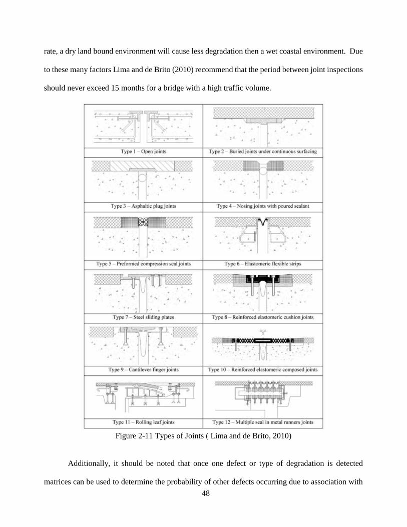
48
rate, a dry land bound environment will cause less degradation then a wet coastal environment. Due
to these many factors Lima and de Brito (2010) recommend that the period between joint inspections
should never exceed 15 months for a bridge with a high traffic volume.
Figure 2-11 Types of Joints ( Lima and de Brito, 2010)
Additionally, it should be noted that once one defect or type of degradation is detected
matrices can be used to determine the probability of other defects occurring due to association with
49
the first defect (Lima and de Brito, 2010). This is additional support for approaching bridge
maintenance with a preventative approach. These defects can be due to a variety of causes, as listed
in detail by Marques Lima and De Brito, in general, however, they can be due to design errors,
manufacturing defects, installation error, a lack of maintenance, a sudden increase in traffic or use,
a change in environmental factors, or sudden impact loads.
Lima and de Brito (2010) propose a rating system for defects in expansion joints. This system
determines the rating in terms of the defect’s severity and thus how detrimental it is to the service of
the bridge. The rating system uses Equation (2.4) below.
Pi = 0.2Iext (6ItIlocCvt + 5Ic) + 2IpCep (2.4)
Where Pi is the rating of the defect i. Each I is an index for defect extent, service life penalty,
traffic penalty, defect location, structure potential penalty, and population penalty respectively,
varying from 0 up to 5 depending on the index and based on increasing severity. The C’s are
coefficients for traffic volume and surrounding population respectively. The numbers correspond to
percent weights for the system such that if every index and coefficient where to be at critical the total
rating would be 100. However in reality the highest rating would be 94 which concerns collapse or
missing joints. Anything higher than 50 is considered very urgent and action should be taken
immediately (Lima and de Brito, 2010). Similarly, if a joint is in perfect condition then the rating
should be equal to zero.
The total degradation of a joint can be classified as Dx, which is the sum of defect ratings, Pi,
of all defects in the joint. See Equation (2.5) below.
Dx = 1
i
n
i
P
(2.5)

50
This equation (2.5) would enable the comparison of multiple expansion joints in the bridge
and therefore the most serious one could be repaired first.
Furthermore, when the expansion joint fails, comes to the end of its design life, or is requiring
excessive and expensive maintenance and repair costs then the joint should be replaced (Savioz,
2014). This is a simple LCCA with fewer costs included, in it the cost of continued maintenance is
compared to the cost of replacement and when the latter becomes the smaller number then
replacement should occur.
The goal throughout all MR&R is to maximize the service life of the expansion joint while
minimizing the cost. This fits directly into the objective of LCCA for bridges. Expansion joints are
a significant part of bridge design, by increasing their life cycle while minimizing maintenance cost
the overall LCC can be decreased.
2.13 Current LCCA Models for Bridges
Over the last few decades several LCCA models for bridges have been developed and
redeveloped. Currently there are three main types of LCCA models, deterministic, rational, and
probabilistic as seen in Figure 2-12 below. Each type has advantages and disadvantages depending
on whether the bridge is new or old, and depending on the available practitioner experience in this
area or access to archived observed deterioration data. Furthermore, each general model type has
overlapping ideas and assumptions, as well as numerous variations developed by various researchers.
The simplest type of LCCA model is a deterministic model, where each contributing cost
constraint is identified, a corresponding cost value is found or estimated for each and the total is
summed. The final LCC is a discrete deterministic result. This method produces an “acceptable
range” but not a detailed or reliability based LCC (Basim and Estekanchi, 2015). This model type

51
does not account for uncertainties, variation, or costs due to unexpected events affecting the bridge
(Reigle and Zaniewski, 2002). The neglect of uncertainties in the deterministic LCCA approach can
cause the results’ validity to be questioned because uncertainty is a part of any future value or cost.
The cost components for costs over the lifespan of the bridge or structure might be the estimated
median cost due to each component (Basim and Estekanchi, 2015) but an average does not account
for probability due to different environments or events. The maintenance cost per year is often a
rough estimate using a specified percentage of the construction cost if there is no historical data to
use. Although if historical data is available that value is preferred. Some costs that are hard to
estimate or predict without data and probability are neglected, these might include some or all costs
associated with users (Kang et al., 2007).
Rational models for LCCA are a combination of deterministic and risk analysis. They
primarily take a deterministic approach but base the cost values on recorded data of similar bridges.
These costs are based on the frequency of a certain cost affecting bridges in similar situations to the
one being analyzed. Marques Lima and de Brito use a rational model for their LCCA, which is
described for expansion joints above in section 2.4. Their model is primarily only for MR&R costs;
however the rational model could be expanded for whole bridge analysis. In general their model uses
a combination of matrices and tables which contain the various bridge or joint components, their
respective rating, and maintenance cost (Lima and de Brito, 2010).
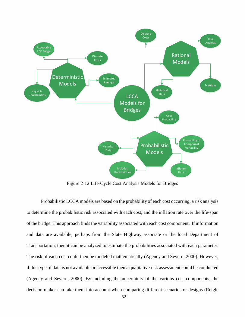
52
LCCA Models for
Bridges
Deterministic Models
Probabilistic Models
Rational Models
Discrete Costs
Acceptable LCC Range
Neglects Uncertainties
Discrete Costs
Risk Analysis
Matrices
Historical Data
Estimated Average
Cost Probability
Inflation Rate
Probability of Component Variability
Includes Uncertainties
Historical Data
`
Figure 2-12 Life-Cycle Cost Analysis Models for Bridges
Probabilistic LCCA models are based on the probability of each cost occurring, a risk analysis
to determine the probabilistic risk associated with each cost, and the inflation rate over the life-span
of the bridge. This approach finds the variability associated with each cost component. If information
and data are available, perhaps from the State Highway associate or the local Department of
Transportation, then it can be analyzed to estimate the probabilities associated with each parameter.
The risk of each cost could then be modeled mathematically (Agency and Severn, 2000). However,
if this type of data is not available or accessible then a qualitative risk assessment could be conducted
(Agency and Severn, 2000). By including the uncertainty of the various cost components, the
decision maker can take them into account when comparing different scenarios or designs (Reigle

53
and Zaniewski, 2002). For most probabilistic LCCA models probability distributions are used and
all costs are brought back to a present worth value using basic net present worth analysis. Using a
present worth analysis accounts for the monetary changes in a life cycle of various components and
combining it with uncertainty analysis can provide a precise LCC (Girmscheid, n.d.).
While some probability analyses rely on analysis of bridge inspection data to form
probabilities for the cost components, other LCCA models use predictive models (Reigle and
Zaniewski, 2002). A probability or risk based LCCA model creates a more universal model because
costs for each component are going to be similar for different bridges, however, the probability will
change based on the environment, location, and conditions. Therefore, if probabilities are developed
for the specific situation, or design, then the LCCA can be conducted for that bridge.
In order to determine the probabilities for a LCCA all possible “hazards and accidental load
scenarios” must be identified before their probability can be found (Agency and Severn, 2000). If
data is not available for analysis and calculation of probabilities then a simple risk interaction matrix
can be used. An example from Agency & Severn is below in Table 2-2. This matrix can then be used
to analyze the hazards and risks associated with a given bridge. Agency & Severn took a 25-year-
old existing bridge as an example and analyze the risks with an interaction matrix as seen in Table
2-3 below. However, if a risk interaction matrix were to be used in a LCCA then the various
classifications of severe, high, medium, low, frequent, occasional, remote, improbable would need
to have probabilities associated with their intersections: unacceptable, tolerable with precautions, and
acceptable. Furthermore, the mitigation for each hazard would need to be quantified as a cost. These
probabilities and costs could then be used in relation to the various hazards to determine the LCC in
the LCCA.

54
Table 2-2 A Risk Interaction Matrix (Agency and Severn, 2000)
Severity Category Likelihood
Frequent Occasional Remote Improbable
Severe U U U U
High U U U T
Medium U T T T
Low T T A A
A = Acceptable T = Tolerable with precautions U = Unacceptable/undesirable
While Agency & Severn’s solution to a lack of reliable data, described above, is workable it
is not as ideal nor as precise as analyzing real inspection data for probabilities. Osman in his report
on “Risk-Based Life-Cycle Costs” discusses this need for reliable inspection data as one of the
disadvantages of Probabilistic LCCA. He cites the need for large amounts of reliable cost and
performance-related data, simulation capability and statistical manipulations as a hindrance to
probabilistic analysis (Osman, 2005). However, this is a limitation for him because he is focused on
private sector design and building.
Federal and State agencies such as state departments of transportation have access to all of
their previous bridge inspections and performance data for various types of brides in different types
of locations. Therefore, if a LCCA is being carried out in the public sphere by either the State
Highway Association or local Departments of Transportation or another company contracted by one
of them, the data should be available for probabilistic analysis.
A newer bridge will have a higher probability of the “do nothing” action (the least severe
action) being chosen because most of its deterioration is minimal and non-serious with respect to the
serviceability of the bridge. The converse would be true of an old bridge which would have a higher
percent of severe deterioration and thus a higher probability of needing repair or replacement. As the
bridge ages and begins to exceed 30 years in service the probability of replacement increases to 100%
quickly (Mao and Huang, 2015). Therefore, these probabilities can be used to determine the LCC for
MR&R costs for a bridge based on its current age and for the rest of its life-cycle.
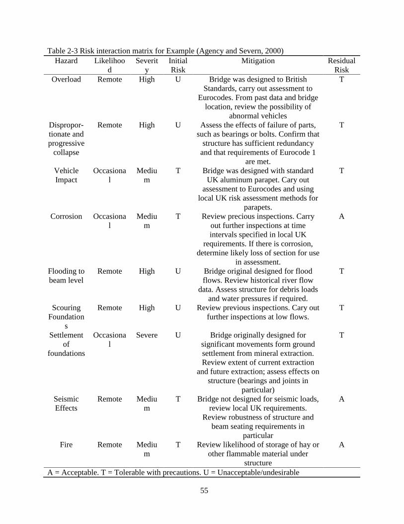
55
Table 2-3 Risk interaction matrix for Example (Agency and Severn, 2000)
Hazard Likelihoo
d
Severit
y
Initial
Risk
Mitigation Residual
Risk
Overload Remote High U Bridge was designed to British
Standards, carry out assessment to
Eurocodes. From past data and bridge
location, review the possibility of
abnormal vehicles
T
Dispropor-
tionate and
progressive
collapse
Remote High U Assess the effects of failure of parts,
such as bearings or bolts. Confirm that
structure has sufficient redundancy
and that requirements of Eurocode 1
are met.
T
Vehicle
Impact
Occasiona
l
Mediu
m
T Bridge was designed with standard
UK aluminum parapet. Cary out
assessment to Eurocodes and using
local UK risk assessment methods for
parapets.
T
Corrosion Occasiona
l
Mediu
m
T Review precious inspections. Carry
out further inspections at time
intervals specified in local UK
requirements. If there is corrosion,
determine likely loss of section for use
in assessment.
A
Flooding to
beam level
Remote High U Bridge original designed for flood
flows. Review historical river flow
data. Assess structure for debris loads
and water pressures if required.
T
Scouring
Foundation
s
Remote High U Review previous inspections. Cary out
further inspections at low flows.
T
Settlement
of
foundations
Occasiona
l
Severe U Bridge originally designed for
significant movements form ground
settlement from mineral extraction.
Review extent of current extraction
and future extraction; assess effects on
structure (bearings and joints in
particular)
T
Seismic
Effects
Remote Mediu
m
T Bridge not designed for seismic loads,
review local UK requirements.
Review robustness of structure and
beam seating requirements in
particular
A
Fire Remote Mediu
m
T Review likelihood of storage of hay or
other flammable material under
structure
A
A = Acceptable. T = Tolerable with precautions. U = Unacceptable/undesirable

56
The probability for each component based on deterioration and the age of the bridge can be
combined to form the many MR&R costs included in the LCCA (Mao and Huang, 2015). Therefore,
for any bridge components the MR&R costs should be correlated to the age of the bridge, and the
fact that their probability will increase as the bridge ages should be taken into consideration in any
LCCA. The costs can be brought to a present value that includes that probability with respect to age.
Another one of the current LCCA approaches was developed for the National Corporative
Highway Research Program (NCHRP). The Bridge Life-Cycle Cost Analysis (BLCCA)
methodology was described in a 2003 report by Hugh Hawk. When it was written, many states had
not yet implemented any form of LCCA, the report was aimed to help more states implement LCCA
approaches in their decision processes. While more states today are using LCCA in their decision
making, the report still provides an excellent description of a general model for LCCA of bridges.
Furthermore, the NCHRP model for BLCCA could provide a useful starting guide for developing a
LCCA model for expansion joints in bridges. NCHRP’s BLCCA model is described below.
Ag
e o
f B
rid
ge (
Yrs
)
Severity of Action Needed
Figure 2-13 MR&R action severity vs Bridge Age

57
First risks and vulnerabilities must be determined for a bridge location and each of those risks
assigned a cost based on the probability of it occurring and consequent costs caused by the risk.
These risks and vulnerabilities could be due to overloads of traffic or equipment on the bridge,
seismic events, bridge scour, partial failure, etc. (Hawk, 2003). Other costs should be estimated as
well. Hawk describes agency costs as including maintenance, rehabilitation, and replacement costs.
Each of the agency costs is affected by material type, condition, environment and location, average
daily traffic, element types, and frequency of maintenance and inspection, among others (Hawk,
2003). User costs and operation costs are also directly related to agency costs and should be analyzed
and determined, user costs were discussed in more detail in section 2.3 above.
The general form of the BLCCA equation is
LCC = DC + CC + MC + RC + UC + SV (2.6)
Where:
LCC = life-cycle cost,
DC = design cost
CC = construction cost
MC = maintenance cost
RC = rehabilitation cost
UC = user cost
SV = salvage value
The BLCCA model’s costs that take place in the bridge’s future are brought to a present
worth value using net present value formulas for uniform series, one time series, gradient series, or
combinations depending on the nature of the cost. This would produce the present LCC for each

58
alternative. In the BLCCA model Hawk describes predicting the distant future as impractical. Instead
he proposes that a specific sequence of maintenance and rehabilitation be analyzed for LCC and then
he suggests that, for analysis purposes that sequence repeats itself endlessly. Eventually the bridge
is replaced and the whole LCCA is repeated. This perpetuated bridge maintenance and rehabilitation
is due to most bridge design life spans being 50 years or more (Hawk, 2003). Furthermore, while
using probability and data for determining the components of the BLCCA equation, it is not
appropriate to assume complete accuracy when approaching the end of the life span of the bridge,
but by using the most current data available an acceptable confidence level might be reached.
2.14 Conclusion
LCCA is critical for cost effective bridge and expansion joint design, with cost components
ranging from initial cost to maintenance and replacement costs. While there are so many factors
affecting the LCC of a bridge, there are many ways to calculate that cost and perform a LCCA, from
a strictly determinate analysis to an analysis based on probabilities. Each model, as discussed above,
has advantages and disadvantages. However, if by taking the best parts of the various models and
building a more comprehensive model for expansion joints based on determinate costs of each
component and a probability of that cost being applied over the life-span of the bridge then a realistic
LCC might be reached. This approach can be used to form a LCCA equation for expansion joints in
bridges, however, it can also be used to form an LCCA equation for replacing expansion joints with
a continuous connection. With these two equations, for an expansion joint that has reached the end
of its life-span and needs to be replaced, the LCCA can be compared for replacing the joint with a
second expansion joint or for retrofitting the joint to be continuous. Then the more economical

59
solution can be chosen based on these LCCs. The equations for each scenario are shown below as
Eq. 7 and 8.
Proposed LCCA model
LCCEJ = f ( Ci + Cc + Co + CmPm + CrPr + CccPcc + CuPu + SV) (2.7)
LCCRC= f ( Ci + CR+ Co + CmPm + CrPr + CccPcc + CuPu + SV) (2.8)
Where:
LCCEJ = Life Cycle Cost of Expansion Joint
LCCRC= Life Cycle Cost of Retrofitted Continuous replacement of joint
Ci = initial cost, fixed cost
Cc = construction cost, fixed cost
CR = retrofitting cost for continuous, fixed cost
Co=cost of operation, fixed cost (only applicable for toll draw bridges)
CmPm=cost of maintenance (function of temp) = (CmHPmH if Temp > 32 ˚F;
CmCPmC if Temp < or = 32 ˚F)
CmPm= composed of maintenance costs of each part of the expansion joint
CrPr = replacement cost (function of temp) = (CrHPrH if Temp > 32 ˚F;
CrCPrC if Temp < or = 32 ˚F)
CrPr = composed of replacement costs of each part of the expansion joint
CccPcc = cost of capital
CuPu = user cost = CdPd+ CvPv+ CaPa
CdPd = driver cost
CvPv = vehicle operation cost
CaPa = accident cost

60
The probabilities, P, for each cost would come from an analysis of the respective Department
of Transportation’s bridge inspection data. The costs, C, for each component would come from the
respective Department of Transportation’s data, typical industry standard costs, related articles, other
LCCA models, and costs for similar products or projects. These probabilities and costs could then
be input into Eq. (2.7) and (2.8) to calculate the LCCAs for each case.
The LCCA for both expansion joints and for retrofitted continuous joints could be determined
and the most cost effective solution chosen for any bridge scenario. While these equations are
primarily designed for analyzing the LCC of joints for existing bridges, the model equations could
easily be adjusted for use on new bridges. The costs and probabilities for each component would
have to be adjusted for the whole bridge instead of for only the joint.
This would expand the number of components with in each overarching cost component,
however the overall process and overarching cost components would remain the same.

61
CHAPTER 3
BRIDGE SELECTION AND FIELD INSTRUMENTATION PLAN
3.1 Introduction
In collaboration with the Colorado Department of Transportation, multiple bridges were
considered for instrumentation to investigate thermal loading and the implications of deck joint
elimination. To correlate the movements detected by the instrumentation as much as possible to those
due thermal effects, specific geometries and characteristics of candidate bridges were desired. The
bridges selected for modeling needed to possess at least one deck joint and simply supported
structural elements that frame into the deck joint. Safe access to bridges for instrumentation purposes
was also an important factor considered when assessing bridge candidates. Bridges with minimal
skew, minimal horizontal curvature, and minimal vertical curvature were sought.
As discussed in Chapter 2, skew and curvature have an effect on the movements of bridges
under thermal loading. However, this study focuses primarily on the vertical thermal gradient. In
order to truly assess how a vertical thermal gradient manifests itself in bridge movement and
performance, it was necessary to minimize the effects that other bridge characteristics would have
on the sensors’ measurements. Therefore, bridges possessing minimal-to-no skew and curvature
were considered for model calibration and deck joint performance assessment.
One concrete and one steel bridge were chosen for field testing and for numerical modeling
in CSi Bridge, a finite element software produced by the maker of SAP2000. An instrumentation
plan was developed to capture the thermal loading throughout the superstructure depth at the
expansion joint and the structural response. Therefore, temperature sensors, strain sensors and
displacement sensors were used on the bridges selected for fine instrumentation. Details of the

62
instrumentation plans for the two bridges chosen to be finely instrumented are discussed further in
Section 3.4.
An additional 16 bridges were chosen to be instrumented across the state of Colorado with
scratch gauges. A scratch gauge is a displacement sensor that was developed by the Colorado
Department of Transportation and manufactured at the Structural Engineering Laboratory at
Colorado State University. It is a non-electronic displacement sensor developed to assess the
influence of regional variations on expansion joint movement. Further details on the scratch gauge
configuration are discussed in Section 3.4.
3.2 Steel Bridge (B-16-FM)
The steel bridge selected for the study, B-16-FM, is located approximately 10 miles north of
Fort Collins, CO and allows County Road 58 to pass over Interstate 25. The proximity to Colorado
State University will give future researchers access to the bridge to troubleshoot any difficulties with
the Data Acquisition System (DAQ) and/or instrumentation sensors. The figure below shows an
aerial view of B-16-FM.

63
Figure 3-1. Plate Girders for Bridge B-16-FM (Google Maps Image)
The bridge possesses three steel plate girders with varying flange thicknesses, bearing and
intermediate stiffeners, and steel diaphragms. Traffic crosses the bridge through one east bound and
one westbound lane. Figure 3-2 the superstructure from under the west abutment of the bridge.
N

64
Figure 3-2. B-16-FM Superstructure from the West Abutment (photo by Authors)
The bridge consists of 4 spans (3 steel spans and 1 short, concrete approach span). The three
steel spans are 74’6” feet in length, simply supported, and separated by expansion joints. Figure 3-3
shows another view of the superstructure and piers. Finger joints, a common type of expansion joint,
shown in Figure 3-4, are in place over the expansion joints to allow thermal movement. The spans
are supported on rocker bearings that transfer the loads to the piers.

65
Figure 3-3. View of B-16-FM from East Abutment (Photo courtesy of CDOT)

66
Figure 3-4. Finger Joint Clogged by Debris on B-16-FM (Photo courtesy of CDOT)
The bridge superstructure was instrumented at the centermost pier, labeled pier 3 by CDOT
nomenclature. Thermocouples, strain gauges, and linear potentiometers were used to collect
information about temperature, strain, and displacement, respectively. In addition to instrumenting
the joint with sensors, an additional strain gauge was placed at the bottom of the web of the plate
girder at mid-span of an adjacent span to validate the finite element model. Data used in calibration
were obtained using control load testing. The test was conducted using a truck with known
dimensions and axle weights, which was provided by CDOT. More information about the control
load testing can be found in Chapter 5.

67
3.3 Reinforced Concrete Bridge (C-17-AT)
A three-span, five-girder traditionally reinforced concrete bridge was chosen as the concrete
bridge for the study. C-17-AT carries northbound Interstate 25 over a gravel service road and is
shown in Figure 3-5 and Figure 3-6 below. The bridge is located approximately 30 miles south of
Colorado State University. The proximity to Colorado State University will give future researchers
access to the bridge to troubleshoot any difficulties with the Data Acquisition System (DAQ) and/or
instrumentation sensors.
Figure 3-5. Aerial View of C-17-AT (Photo courtesy CDOT)
Bridge
Location

68
Figure 3-6. C-17-AT (Photo courtesy CDOT)
The concrete girders are traditionally reinforced, the spans are simply supported, and two
expansion joints separate the three spans. Extensive corrosion and damage is observable below the
deck joints. Figure 3-7 shows the discoloration of the pier caps that are directly below the expansion
joints.

69
Figure 3-7. Discoloration under expansion joint on C-17-AT (Photo courtesy CDOT)
3.4 Field Instrumentation
Since the process of field instrumentation is general for both bridges, the logistics for Bridge
C-17-AT only are discussed. C-17-AT is a three span, five girders, and two expansion joint
traditionally reinforced concrete bridge, C-17-AT, carries Northbound I-25 over a gravel access road
that connects frontage roads. These can be seen in Figure 3-8 and Figure 3-9 below. Located
approximately 30 miles south on I-25 of Colorado State University, the bridge is close enough to
provide easy access for field implementation and for researchers in the event of repairs or remediation
needed by either the Data acquisition system (DAQ) or the sensors.

70
The spans are each approximately 31 ft long and 42 ft wide, with expansion joints separating
the three spans. See Appendix A for drawings. Each of the five girders, as well as the deck are
traditional reinforced concrete, they are also simply supported. Pier caps and columns are also
reinforced concrete. Furthermore, extensive damage and corrosion and leakage from the expansion
joint can be seen on the underside of the girders and expansion joints. See Figure 3-10 below.
The expansion joints are simple joints with a rubber silicone seal, however, the seal was
cracked and the joint was clogged with visible clogging and deterioration on the ends. See Figure
3-11 and Figure 3-12 below showing the clogging present in the expansion joint at the time of
instrumentation.
Figure 3-8 C-17-AT Overview
N
I-2
5N
I-2
5S
NE
FR
ON
TA
GE
RO
AD
Instrumented Joint
C-17-AT
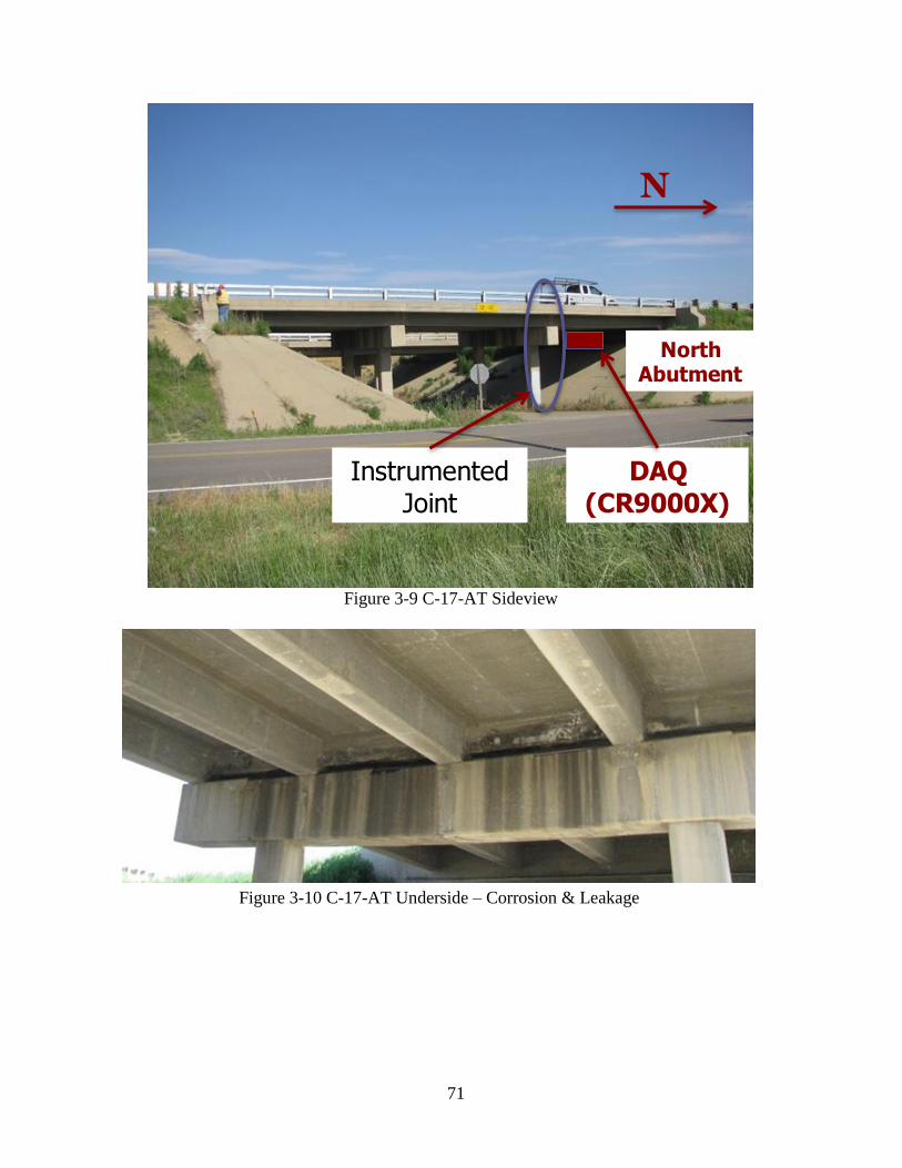
71
Figure 3-9 C-17-AT Sideview
Figure 3-10 C-17-AT Underside – Corrosion & Leakage
DAQ(CR9000X)
N
North Abutment
Instrumented Joint
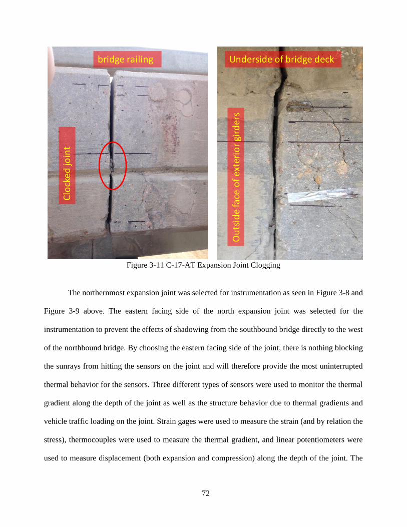
72
Figure 3-11 C-17-AT Expansion Joint Clogging
The northernmost expansion joint was selected for instrumentation as seen in Figure 3-8 and
Figure 3-9 above. The eastern facing side of the north expansion joint was selected for the
instrumentation to prevent the effects of shadowing from the southbound bridge directly to the west
of the northbound bridge. By choosing the eastern facing side of the joint, there is nothing blocking
the sunrays from hitting the sensors on the joint and will therefore provide the most uninterrupted
thermal behavior for the sensors. Three different types of sensors were used to monitor the thermal
gradient along the depth of the joint as well as the structure behavior due to thermal gradients and
vehicle traffic loading on the joint. Strain gages were used to measure the strain (and by relation the
stress), thermocouples were used to measure the thermal gradient, and linear potentiometers were
used to measure displacement (both expansion and compression) along the depth of the joint. The
Ou
tsid
e fa
ce o
f ex
teri
or
gird
ers
Underside of bridge deckbridge railingC
lock
ed jo
int

73
placement of these sensors on the joint can be seen in Figure 3-13 below (See Appendix B for more
details) and their details are discussed in Sections 3.2.1, 3.2.2, and 3.2.3 respectively.
Figure 3-12 C-17-AT Expansion Joint Deterioration
The bridge was instrumented August 22nd through the 24th, 2016. The overall instrumentation
process was smooth, with only minor adjustments needed in field such as running the wires along
the bridge railing instead of along the bottom of the girder. Due to the bridge carrying northbound I-
25, the running of the wires along the railing was done at night, 9pm, on August 23rd, 2016 in order
to utilize a night-time construction lane closure.
Outside face of exterior girders
Un
der
sid
e o
f bri
dge
dec
k
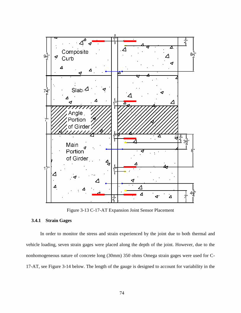
74
Figure 3-13 C-17-AT Expansion Joint Sensor Placement
3.4.1 Strain Gages
In order to monitor the stress and strain experienced by the joint due to both thermal and
vehicle loading, seven strain gages were placed along the depth of the joint. However, due to the
nonhomogeneous nature of concrete long (30mm) 350 ohms Omega strain gages were used for C-
17-AT, see Figure 3-14 below. The length of the gauge is designed to account for variability in the

75
material’s response, through averaging of the measurement along the gauge length, and thus provides
a more representative strain reading.
Figure 3-14 Concrete Strain Gage
Two strain gages were placed approximately one inch from the top of the slab on either side
of the expansion joint to provide redundancy. One was placed approximately one inch above the
bottom of the slab on the north side of the joint. One was placed on the girder approximately one
inch below the slab on the north side of the joint. A fifth was placed halfway down the girder on the
north side of the expansion joint. The two final gages were placed on either side of the joint
approximately one inch above the bottom of the girder. These can be seen in Figure 3-13 above.
The concrete was ground smooth with a grinder before the strain gages were applied to the
concrete of the slab and girders with a strong epoxy glue. The smooth surface provided by the grinder
ensures full contact between the sensor and the concrete. Once glued to the slab and girders the
strain gages were soldered to their corresponding labeled wires. Soldering was done in field due to
the length of the strain gages. With shorter/smaller strain gages soldering can be completed in the
lab and the gages can be brought to the field already connected, however, the longer strain gages
needed for the concrete are more bendable and fragile than smaller ones use for steel. Thus, soldering
before application introduces unreasonable risk of damage to the strain gage. This application process
can be seen in Figure 3-15 and Figure 3-16 below. Once the strain gage was soldered to the wires in

76
the field, the resistance at the other ends of the wires was tested to ensure proper connection to the
strain gage. Extra strain gages were available in the event that soldering was improper and unfixable,
in which case a new strain gage would have been applied and soldered and tested. Once the strain
gages were fully installed and tested, they were covered by an adhesive rubber protective cover that
was additionally caulked along the edges to ensure protection from the elements.
Figure 3-15 Strain Gage Application
Figure 3-16 Strain Gage Protection

77
3.4.2 Thermocouples
Thermocouples were used to monitor the thermal distribution throughout the depth of the
expansion joint. Omega type K thermocouples were chosen; they are self-adhesive and designed to
resist the outdoor elements. Their flexible design allows for full contact with the material and a large
temperature range of -58 to 392°F. These are the same thermocouples used for bridge B-16-FM, and
have provided consistent data for that bridge supporting the decision to use the type of thermocouples
for bridge C-17-AT.
Four thermocouples were used along the depth of the expansion joint to record and monitor
the thermal gradient along the joint. One thermocouple was placed approximately two inches below
the top of the slab, or approximately one inch below the strain gage on the north side of the joint. A
second one was placed approximately two inches below the bottom of the slab on the girder (about
1 inch below the strain gage). A third thermocouple was placed at mid depth on the north girder
approximately 1 inch below the mid depth strain gage. A final thermocouple was placed
approximately 2 inches above the bottom of the north girder, about 1 inch above the bottom strain
gage. Their placement can be seen in Figure 3-13 above.
The concrete was also ground smooth with a grinder before the thermocouples were applied
by peeling off the protective cover and pressing the adhesive side to the concrete, as shown in Figure
3-17 below. Once the thermocouple is firmly attached, the wires were connected using thermocouple
wire connection plugs, which were prewired to the thermocouple and the shielded wires before
instrumentation. These connection plugs are specific to type K thermocouples and provide a fully
secure, protected, and complete connection between the thermocouple and the wire and thus the
DAQ. These connectors can be seen in Figure 3-18 below and help ensure accurate data is recorded.

78
Figure 3-17 Thermocouple Application
Figure 3-18 Thermocouple Connectors
3.4.3 Linear Potentiometers
Measuring the displacement of the joint in both directions, expansion and contraction, is the
primary indication of how critical the expansion joint is to the bridge as well as the effects of clogging

79
and thermal gradient changes on the bridge. To measure these displacements, Celesco model CLP
50 linear potentiometers were chosen. These linear potentiometers can measure up to one-inch
extension and one-inch compression, for a total of two inches of displacement. The linear
potentiometer in Figure 3-19 below is shown extended to its full two-inch extension. This model has
a life expectancy of 25 million repetitions and is designed to resist environmental elements, including
a temperature range of -40˚ to 212˚F and up to 20000 Hz of vibration. These were the same linear
potentiometers that were used on B-16-FM and have provided consistent and continuous
displacement data from that bridge.
Figure 3-19 Extended Linear Potentiometer
Three of these linear potentiometers are used on the north joint of C-17-AT. The first was
placed across the joint at mid depth on the slab, approximately 3.75 inches below the top of the slab.
The second linear potentiometer was placed across the joint on the girders approximately 3.75 inches
below the bottom of the slab. The last linear potentiometer was placed across the joint on the girders
3.75 inches above the bottom of the joint. Their placement can be seen above in Figure 3-13.
In order to ensure full extension and compressibility of the linear potentiometers across the
joint, the linear potentiometers were mounted on mounts made of a square of Plexiglas with a bolt
through the middle which was then ran through the ring on the end of the linear potentiometer and
secured with a nut, see Figure 3-20 below. The concrete was ground smooth with a grinder before
the mounts were glued to the girder with the same epoxy that was used for the strain gages. When

80
mounting the linear potentiometers, measurements were made and marked on the concrete, next the
mounts were glued in placed. The epoxy only takes a couple minutes to harden and once hardened
the linear potentiometers were attached and bolted in place, see Figure 3-21 below. Finally, the linear
potentiometer was covered with half of a PVC pipe to the sensor from weather. The PVC pipe was
only attached on one side of the joint to ensure free movement of the joint and sensor. The PVC
covered linear potentiometer can be seen in Figure 3-22 below.
Figure 3-20 Linear Potentiometer Mount

81
Figure 3-21 Linear Potentiometer in Place on Joint
Figure 3-22 PVC covered Linear Potentiometer
3.4.4 Wires
Shielded wires were used for all sensors to protect the data from the elements and minimize
noise in the data collected. Two types of shielded wires were used. Thermocouples wired over

82
distanced greater than a few feet require shielded thermocouples wires that will transmit the
temperature over the longer distances and protect it from the elements. Thus, Type K Omega
extension thermocouple wires were used. These wires have a polyvinyl shield, a max temperature of
221˚F, and solid wires, with a 16 AWG No, these wires can be seen in Figure 3-23 below.
Figure 3-23 Shielded Thermocouple Wire
For the strain gages and linear potentiometers, shielded wires from Allied Wire and Cable
were chosen. The FR-EPR/CPE Instrumentation Cable with individual and overall shielded pairs.
These wires have AWG No. 18, with two pairs of wires. The wires have copper drain wires that
were grounded to minimize noise, Ethylene propylene Rubber (FR-EPR) insulation, and shields of
aluminum with overall covers of chlorinated Polyethylene (CPE). The have a max temperature of
194˚F and voltage of 600V. These double shielded wires are shown below in Figure 3-24.
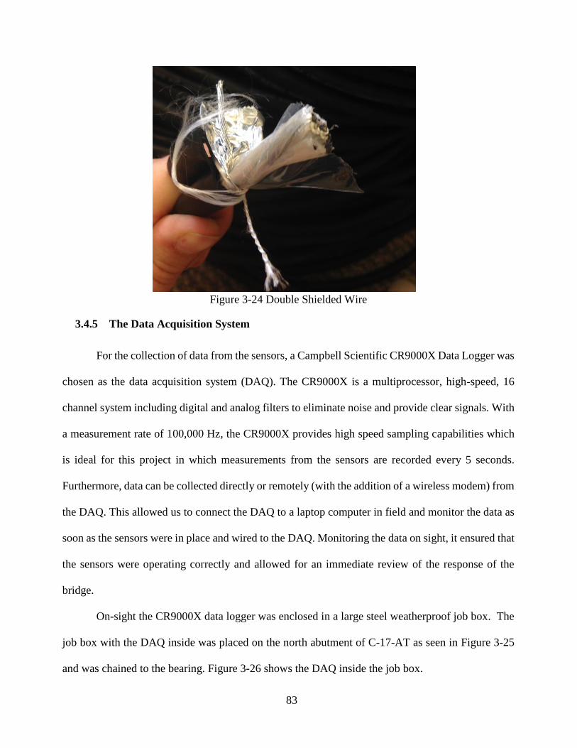
83
Figure 3-24 Double Shielded Wire
3.4.5 The Data Acquisition System
For the collection of data from the sensors, a Campbell Scientific CR9000X Data Logger was
chosen as the data acquisition system (DAQ). The CR9000X is a multiprocessor, high-speed, 16
channel system including digital and analog filters to eliminate noise and provide clear signals. With
a measurement rate of 100,000 Hz, the CR9000X provides high speed sampling capabilities which
is ideal for this project in which measurements from the sensors are recorded every 5 seconds.
Furthermore, data can be collected directly or remotely (with the addition of a wireless modem) from
the DAQ. This allowed us to connect the DAQ to a laptop computer in field and monitor the data as
soon as the sensors were in place and wired to the DAQ. Monitoring the data on sight, it ensured that
the sensors were operating correctly and allowed for an immediate review of the response of the
bridge.
On-sight the CR9000X data logger was enclosed in a large steel weatherproof job box. The
job box with the DAQ inside was placed on the north abutment of C-17-AT as seen in Figure 3-25
and was chained to the bearing. Figure 3-26 shows the DAQ inside the job box.

84
Figure 3-25 Job Box on North Abutment’
Figure 3-26 DAQ in Job Box
The wires were run from the sensors on the north joint along the top of the bridge to the job
box. The wires were connected to the railing along the west edge of the bridge using zip ties and
protected by halved PVC pipes to provide uniformity and security. The wires were then run through
a gasket on the side of the job box and connected to the CR9000X data logger inside. The wires
running along the bridge are shown in Figure 3-27 below.

85
Figure 3-27 Wires Along Railing
The DAQ system is powered by a size 27 deep cycle marine battery that is charged by a 70
Watt solar panel. The battery is stored inside the job box next to the CR9000X as seen in Figure
3-26 and connected via wires to the positive and negative terminals in the CR9000X. The solar panel
was installed a month and a half after sensor installation due to shipping time. During the interim
period the battery was charge using a battery charger about once each week. The solar panel was
placed at a 45-degree angle to maximize sunlight exposure throughout the year and was installed on
the west side of the north abutment. The solar panel is wired to a charge controller which is then
connected to the battery. The charge controller prevents the battery from becoming over charged.
The solar panel installation is discussed in Section 3.4 below.
3.5 Remote Data Collection
Two methods were available for data collection from the CR9000X. The DAQ stores data on
a 2 GB memory card, which can hold several months of data. The first method of collection would
be by going out to the bridge periodically for collection by hardwiring a laptop to the DAQ and
downloading the data from the memory card. The second option would be connecting a wireless

86
modem to the CR9000X data logger and then downloading the data remotely from the DAQ to an
office computer using a static IP address.
The second method was chosen as more convenient and economical. Not only would a
wireless connection to the DAQ make data collection easier, it would also allow the researchers to
check on the sensors remotely. This would ensure that sensors are working properly, thus allowing
researchers to easily see when a sensor might need attention or mediation in field.
The Campbell Scientific RavenXTV modem was chosen for wireless data collection. This
modem is designed to work with the CR9000X data logger and a Verizon IP address. A static IP
address was chosen to provide easier access to the data. Once the Verizon static IP address was set
up and assigned to the modem the modem was configured using provided software and was plugged
into the CR9000X data logger on-sight. Figure 3-28 shows the modem connected to the data logger
and Figure 3-29 show the modem’s antenna attached to the side of the bridge. For collection the
software RTDAQ was used to connect remotely to the CR9000X via the modem and IP address.
Once connected, data can be downloaded and saved as .csv files and analyzed. Data is collected,
downloaded, and converted once a week to minimize any backup of data and streamline the analysis
process discussed in Chapter 4.
Figure 3-28 RavenTXV Modem

87
Figure 3-29 Modem Antenna
3.6 Solar Panel Installation
The location of bridge C-17-AT does not provide access to electricity, consequently
alternative sources of energy for powering the CR9000X system were considered. First, rechargeable
batteries were considered. These would be switched out and recharged by either CSU or CDOT
personnel. The second option considered was a rechargeable battery charged by solar panel attached
to the abutment. This second option proved to be both more cost and time effective because it would
not require regular trips out to the bridge. The cost of the solar panel proved to be comparable to a
second rechargeable battery and significantly cut maintenance hours. The battery chosen is a deep
cycle 12 Volt marine battery, a Diehard Group 27M. The solar panel chosen is a Newpowa 70-Watt
panel with a 12-Volt solar charge controller to prevent over charging of the battery. The solar panel
weighs 13 pounds and is 30.48 in x 26.57 in x 1.18 in and is shown in Figure 3-30 below.

88
Figure 3-30 Solar Panel, 70 Watt
A frame to hold the solar panel at a 45-degree angle against the abutment was built out of
2x4s. Positioning the solar panel at a 45-degree angle allows for maximum sunlight ray absorption
throughout the calendar year based on sun ray angles. The frame 2x4s were connected to the solar
panel using screws and brackets as seen in Figure 3-31 below. The ends of the frame were attached
to brackets which would be attached to the concrete abutment using screws. The in place solar panel
is shown in Figure 3-32 below.
The solar panel was installed on October 8th, 2016. The panel was installed after the rest of
the instrumentation due to shipping time constraints. During the interim between instrumentation
and solar panel installation, the battery was picked up once every eight days to be charged and then
returned to the sight. The panel was installed by using a pachometer to detect rebar in the abutment,
the locations of the screws were then marked and holes drilled into the concrete. The solar panel was

89
then put in place and the frame screwed into the concrete. Once in place, the solar panel wire was
connected to the charge controller and that to the battery providing power to the DAQ.
Figure 3-31 Solar Panel Frame
Figure 3-32 Solar Panel Attached to Abutment

90
CHAPTER 4
CONTROLLED LOAD TEST MODEL VALIDATION
4.1 Introduction
In order to validate the finite element model of the bridges, static control load test was
performed following the completion of the field instrumentation. The test was performed by parking
a truck with known dimensions and axle weights on the bridge and strain data was collected. The
test was performed in two parts, first with the front axle directly above the mid-span strain gage, and
second with the back axles centered above the mid-span strain gage. The same truck loads were
placed on the finite element model and the two responses were compared.
4.2 Test Vehicle Information
The truck used for the control load test was an Aspen Aerials A-40 Bridge Inspection Unit
Truck, which was provided and operated by CDOT personnel. This was the same truck that was used
for sensor installation on the bridge. The axel weights and dimensions for the A-40 truck can be
seen below in Figure 4-1. These axle weights are for when the inspection bucket arm is fully
contracted and stowed on the bed of the truck. These axle weights are accurate to within +/- 2% of
the exact weight, according to the manufacture. The position shown, with bucket arm fully contracted,
is how it was parked on the bridge for the test.

91
Figure 4-1 Aspen Aerials A-40 Truck with Dimensions and Axel Weights
4.3 Model and Predictions
The effect of the Aspen Aerial A-40 truck was included in the finite element model of bridge
by inputting the axel weights as point loads representing the tires in the same location as in field test
scenarios. Two scenarios were considered: 1) when the truck was parked with its front axle at the
mid-span location and 2) when the truck was parked with its two back axles over the mid-span
location.
The strain gauge at mid-span, for both bridges, was monitored during the truck load tests and
used for validating the numerical model. For the reinforced concrete bridge, this strain gauge was
installed about 2 inches above the bottom of the outside west girder at mid-span. For the steel bridge,
the gauge was installed on the centermost girder
For the concrete bridge, the first scenario in the finite element model, where the front axle is
above mid-span, gives the stress at the bottom of the girder at mid-span to be 0.146 ksi. The second
scenario, when the back axles are centered above mid-span, gives the stress at the bottom of the
girder at mid-span to be 0.349 ksi. For the steel bridge, when the front axle is located at the mid-span

92
of the bridge in the finite element model, the stress on the top of the bottom flange at mid-span is
1.39 ksi. When the back axles are split across the mid-span, the model predicts the stress on the top
of the bottom flange at mid-span to be 2.20 ksi.
4.4 Results and Comparison to the Finite Element Models
4.4.1 C-17-AT
Each of the two scenarios of the control load test were performed for approximately one to
two minutes. During each of these tests the data was collected in field at 5 second intervals from the
strain gauge at mid-span. Collecting several data points over the span of the test allowed for a moving
average to be applied to the data. These average strains were then converted to stress and compared
to the corresponding finite element model stresses. Figure 4-2 and Figure 4-3 shows some of the data
collected for the front axle test and for the back-axle tests respectively.
Figure 4-2 Front Axle Control Load Test Data

93
Figure 4-3 Back Axle Control Load Test Data
An average of the data collected during the field test was used to calculate the average micro
strain for each of the two scenarios. The front axle scenario gave an average micro strain at mid-span
of 30.18. The back axles gave an average micro strain at mid-span of 73.69. These micro strains
were converted to stresses using the modulus of elasticity of the concrete, 3604 ksi. Table 4-1 below
shows both the predicted stresses from the numerical model and the measured field response stresses.
Table 4-1 also shows the calculated percent difference between the predicted and measured stresses.
A percent difference less than 20% is considered good, and as shown good agreement was achieved
between the field test and the numerical model.
Table 4-1. Comparison of Field Stress and Model Stress Predictions
Front Axle at Mid-span Back Axles at Mid-span
Predicted Stress (ksi) 0.146 0.349
Measured Stress (ksi) 0.109 0.266
Percent Difference (%) 11.5 9.74

94
4.4.1 B-16-FM
Control load tests were performed with the front axle at mid-span and again with the rear
axles at mid-span to match the scenarios that were modeled. During each test the data from the mid-
span strain gauge was collected in the field at five second intervals for approximately one minute.
Some noise in this data was expected due to the length of the wires being approximately 240 ft.
Collecting several data points allowed a moving average to be applied to the data to determine the
actual strain. Figure 4-4 shows the microstrain at mid-span when the truck was parked with its front
axles at mid-span. Figure 4-5 shows the microstrain at mid-span when the truck was parked with its
rear axles at mid-span.
Figure 4-4. Field Control Load Test with Front Axle of A-40 Truck at Mid-Span
0 10 20 30 40 50 60 70 80 90 100 110-60
-45
-30
-15
0
15
30
45
60
75
90
105
Time (seconds)
Mic
rostr
ain
at M
id-S
pa
n
Truck On Bridge
Truck Not On Bridge

95
Figure 4-5. Field Control Load Test Microstrain with Back Axles at Mid-Span
A simple average of the data collected was used to determine the average microstrain for
each scenario. The average microstrain when the front axle was located at mid-span was 47.36
while the average microstrain when the back axles were located at mid-span was 71.99. The
microstrains were converted into stress using the modulus of elasticity. Table 4-2 shows the
comparison of the model predictions to the measured field response. As shown in the table,
excellent agreement was achieved.
Table 4-2. Comparison of Field Stress to Modeled Stress Predictions
0 10 20 30 40 50 60 70 80 90 100
-45
-30
-15
0
15
30
45
60
75
90
105
Time (seconds)
Mic
rostr
ain
at M
id-S
pa
n
Truck On Bridge
Truck Not On Bridge
Front Axles at
Mid-span
Back Axles at
Mid-span
Predicted Stress (ksi) 1.39 2.20
Measured Stress (ksi) 1.37 2.09
Percent Difference (%) -1.22% -5.10%

96
CHAPTER 5
DATA ANALYSIS FOR BRIDGE C-17-AT
5.1 Introduction
The data from the bridge was downloaded weekly and a brief analysis performed using an
analysis and plotting code written in RStudio (2016). The data was visualized and analyzed to
determine patterns and correlations between the thermal, displacement, and strain/stress data. The
analysis was conducted in order to discern how much movement, stress, and temperature change the
bridge is experiencing. This knowledge is used to enhance understanding of the expansion joints on
the bridge’s overall health and LCC. The correlations and patterns are used to draw conclusions about
the impact of the clogged joint and of the thermal gradients through the depth of the bridge. The
thermal gradients measured are also compared to standard thermal gradients for further analysis.
This data and analysis was finally used to form recommendations for joint removal and retrofitting.
5.2 Analysis Plotting Code
The analysis code for the C-17-AT and B-16-FM data was written in RStudio in order to
provide easy comparison and visualization of the data. The code was divided into three sections. The
first section provided a general analysis and comparison of the sensors’ data by producing a three-
part graph. The second section provided a comparison of the maximum temperature difference and
the stress by producing a two-part graph. The third section calculates the minimum, average, and
maximum thermal gradients through the depth of the bridge and plots them next to each other on a
three-part graph for comparison to the standard temperature gradients of AASHTO and New Zealand.

97
The data is downloaded from the DAQ through the wireless RAVEN XTV modem as .dat
files. These .dat files are then converted to .csv files and both are saved and backed up. The code
works by reading in the appropriate files as .csv files. The user then selects the date range, desired
sensors, and sets the plotting parameters. Next the code is run and the plots simulated. Finally, the
plots are saved and analyzed.
5.3 Sensor Correlation and Patterns
Due to bridge C-17-AT’s location in Colorado where there is a large range of temperatures,
a maximum range of 140 ̊F (60 ̊C) over the course of the year, the bridge is likely to experience
significant differences in temperature (AASHTO, 2012). Thermal gradients are usually most
uneven at times of heating or cooling of the bridge, especially during times of direct sunlight. Heat
transfer due to direct radiation from the sun, conduction, or convection occurs every time that the
ambient air temperature varies – typically every morning and evening. Multiple parameters affect
how evenly the bridge loses and gains heat, including bridge orientation, length of concrete overhang,
depth of girders, height of concrete slab, and girder spacing (Chen, 2008).
The coefficient of thermal expansion, commonly expressed as µ or α, describes the
increase in length of a material for a given increase in temperature. A negative result for the
change in length corresponds to a shortening of the material and conversely a positive value
corresponds to an increase in material length. Bending stresses can develop through the depth of
the bridge due to the presence of thermal gradients causing the concrete deck and girder to expand
at different rates.
The five months in which data has been collected to date on the C-17-AT bridge provide a
foundation for preliminary conclusions about temperature’s effect on the expansion joint and allows

98
for comparison to theoretical expectations. The displacement experienced by the expansion joint
should be closely correlated with the effective temperature experienced by that joint. This was found
to be true in the research monitoring conducted by Y. Q. Ni et al. (2007) on the Ting Kau Bridge. It
was also found that the correlation could be predicted using a linear regression model (Ni et al.,
2007). However, only the effective temperature, which is the weighted average temperature
throughout the depth of the bridge, was considered, rather than the exact temperature at each point
through the depth of the bridge. The study also did not include monitoring of stress and strain at the
expansion joint. When evaluating the data from C-17-AT over the course of these first five months,
similar correlations are seen between the temperature, stress and displacement. Figure 5-1 below
shows a two-week span of the C-17-AT data at the end of October and shows a distinct converse
pattern between the temperature data plotted in (a) and the displacement data plotted in (b). As the
temperature rises the displacement decreases, i.e. the girders expand and the joint closes; conversely
as the temperature falls, the displacement increases, i.e. the girders contract and the joint opens
further. This behavior of the joint, in conjunction with the temperature, confirms that the joint is
directly affected by the changing temperature. A fainter pattern can be determined between the stress
(from the strain gauges) in (c) and the temperature and displacement data. During the first half of the
data set the temperatures show a greater range (about 15 degrees) and higher average compared to
the second half, also during the first half the stress data shows more variance and during the second
half is more constant. Additionally, the displacement changes less during the second half as well,
showing that the greater the range of temperature experience in a short time period the greater the
displacement changes and the large the effect on the stresses in the bridge.
The impact of the daily temperature range can be further seen by looking at close up of the
data during smaller range period and a larger range period. Figure 5-2 below shows data from C-17-
AT from November 30th through December 2nd and Figure 5-3 below shows data from October 15th

99
through October 18th. In Figure 5-2 the temperature range is only approximately 10 degrees and the
displacement in (b) shows minimal change, a maximum of 0.05 inches of change in displacement.
The stress also shows very little change in (c). On the other hand, looking at Figure 5-3, the
temperature range is around 15 degrees and the displacement (b) shows a little more change, a
maximum of about 0.09 inches and the stress (c) shows some variance. All of which indicates the
importance of the temperature range on the joint and bridge’s overall health.
Figure 5-1 C-17-AT Bridge Sensor Data Oct.15th through Oct. 30th, 2016
(a) Thermocouple Data, (b) Linear Potentiometer Data, (c) Change in Stress Data.
Note: ̊C = ( ̊F – 32)/1.8; 1 in = 25.4 mm; 1psi = 6.89 kPa

100
Figure 5-2 C-17-AT Bridge Sensor Data Nov.30th through Dec. 2nd, 2016
(b) Thermocouple Data, (b) Linear Potentiometer Data, (c) Change in Stress Data.
Note: ̊C = ( ̊F – 32)/1.8; 1 in = 25.4 mm; 1psi = 6.89 kPa
Furthermore, these patterns and relationships between temperature and joint displacement
and stress can be seen more distinctly in data from the steel girder bridge, B-16-FM. The B-16-FM
bridge’s data shows these relationships more clearly for two reasons. First, is due to the data being
collected during times of greater temperature ranges and second is due to the nature of the bridge
because the girders are steel in B-16-FM, on rollers, the bridge is under more direct sunlight, and the
joint is more severely clogged. Figure 5-4 below shows some data from B-16-FM that confirms the
same relationships seen in C-17-AT’s data above. When evaluating the middle portion of Figure 5-4
one can see that the temperature is varying very little as are the displacement and stress compared to

101
either end of the data were significantly greater temperature ranges and variance in displacement and
stress are observed.
Figure 5-3 C-17-AT Bridge Sensor Data Oct.15th through Oct. 18th, 2016
(c) Thermocouple Data, (b) Linear Potentiometer Data, (c) Change in Stress Data.
Note: ̊C = ( ̊F – 32)/1.8; 1 in = 25.4 mm; 1psi = 6.89 kPa
From these initial correlations, it can be concluded that not only is the temperature change
affecting both the expansion joint’s movement but also the stress experienced in the vicinity of the
joint. When the temperature has a similar daily variation of around or less 10 degrees the average
stress varies by less than 0.25ksi for the concrete bridge and 3 ksi for the steel bridge and
displacements vary by about 0.02 in and 0.5 inches respectively. However, when the daily
temperature range changes from day to day and is larger (15 degrees or more), the joint experiences
larger stress and displacement shifts. These larger daily temperature shifts cause stresses to vary by
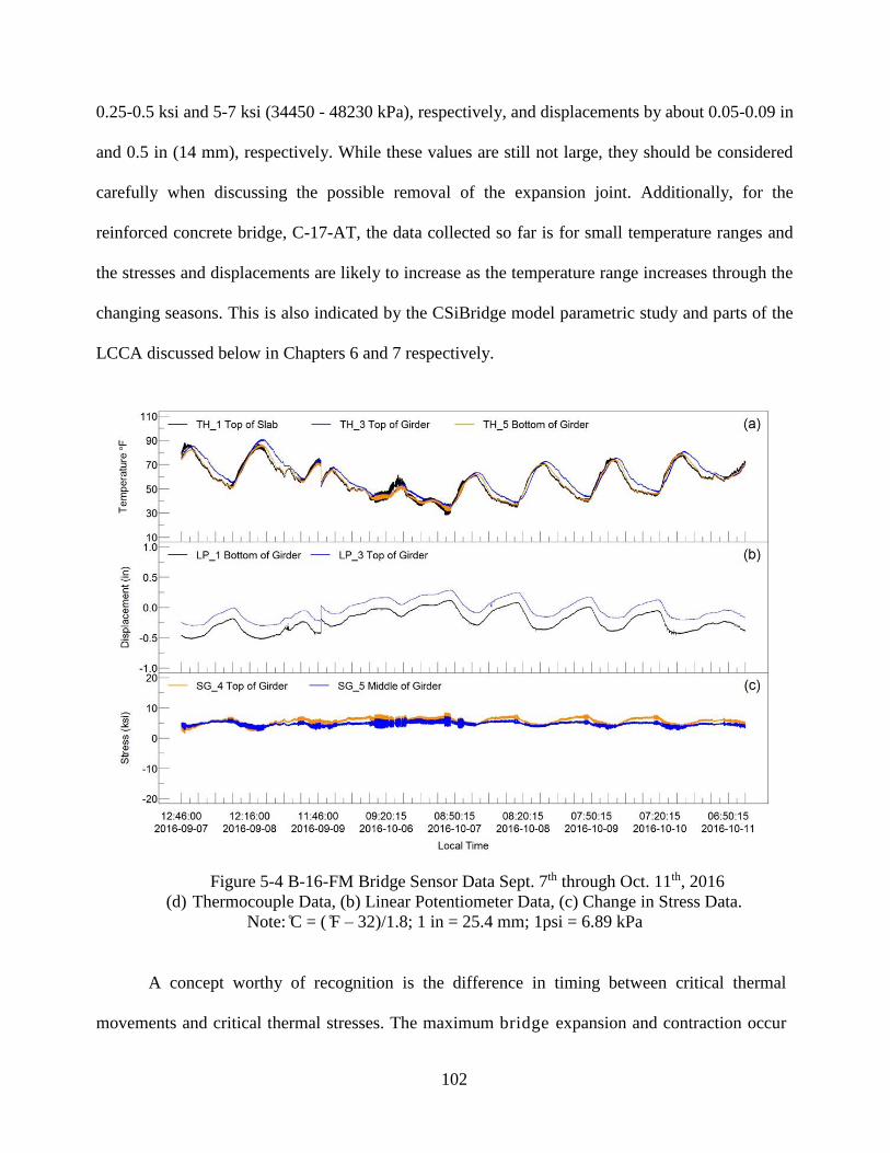
102
0.25-0.5 ksi and 5-7 ksi (34450 - 48230 kPa), respectively, and displacements by about 0.05-0.09 in
and 0.5 in (14 mm), respectively. While these values are still not large, they should be considered
carefully when discussing the possible removal of the expansion joint. Additionally, for the
reinforced concrete bridge, C-17-AT, the data collected so far is for small temperature ranges and
the stresses and displacements are likely to increase as the temperature range increases through the
changing seasons. This is also indicated by the CSiBridge model parametric study and parts of the
LCCA discussed below in Chapters 6 and 7 respectively.
Figure 5-4 B-16-FM Bridge Sensor Data Sept. 7th through Oct. 11th, 2016
(d) Thermocouple Data, (b) Linear Potentiometer Data, (c) Change in Stress Data.
Note: ̊C = ( ̊F – 32)/1.8; 1 in = 25.4 mm; 1psi = 6.89 kPa
A concept worthy of recognition is the difference in timing between critical thermal
movements and critical thermal stresses. The maximum bridge expansion and contraction occur

103
at the joint during the warmest days in summer and the coolest nights in winter, respectively.
However, the maximum thermal stresses due to the presence of thermal gradients through the
depth of the superstructure occur during the warming of the bridge in the early afternoon or the
cooling of the bridge in the evening rather than that in the morning (Moorty, 1992). Verification of
this concept and further understanding of the heating and cooling cycles on Colorado bridges
can be further understood with temperature data from instrumentation of in-service bridges such as
C-17-AT and B-16-FM.
Although current AASHTO provisions only require consideration of total longitudinal
thermal movement based on average bridge temperatures, stresses due to temperature differentials
in the cross section were shown to commonly be above +/- 5 ksi (34450 kPa) in steel box girder
bridges in Texas (Chen, 2008). Though different girder material, widths, depth and bridge location
would change the value of these stresses as shown above, it is clear that the significance of these
stresses is worth analysing in Colorado’s reinforced concrete and steel bridges.
The significance of the thermal gradient across the depth of the bridge is justified not only
through the correlation between the temperature measurements and corresponding stresses, but also
by calculating and comparing the maximum temperature difference. The maximum temperature
differential through the depth of the bridge was calculated from the thermocouple data and compared
to the stresses experienced by the bridge in Figure 5-5 below. The peaks in stress correlate with the
larger magnitude temperature differences. Furthermore, the warmer the season becomes the greater
the maximum difference in temperature across the girder’s depth and the greater the stresses
experienced.

104
Figure 5-5 Maximum Temperature Difference Through Depth vs Stress Data.
(a) Max Temperature Difference, (b) Change in Stress Data.
Note: ̊C = ( ̊F – 32)/1.8; 1 in = 25.4 mm; 1psi = 6.89 kPa
5.4 Thermal Gradients and Bridge Deterioration
The next step is to compare these thermal gradients through the depth of the joint to standard
design gradients. First, the temperature gradient with the minimum temperature and the average of
the temperature gradients in the 10th percentile of measured temperature and second the temperature
gradient with the maximum temperature and the average of the temperature gradients in the 90th
percentile of measured temperature were plotted to see what shape the thermal gradient formed on
the joint as seen in Figure 5-6 (c) below. The standard thermal gradients were also plotted on the
depth of the girder for full comparison. What is initially apparent is that the minimum and maximum
gradients have opposite shapes, as seen in Figure 5-6 (c), although the maximum temperature

105
gradient has a more gradual slope when compared to the minimum. Nonetheless, when compared to
the shape of the New Zealand and the AASHTO Standard Temperature gradients as shown in Figure
5-6 (a) and (b) respectively, they do not match (AASHTO, 2012; New Zealand, 2013).
Figure 5-6 Design Standard vs. Measured Temperature Gradients.
(a) New Zealand (mm) (17), (b) AASHTO (in) (1), (c) Measured Temperature
Gradients. Note: ̊C = ( ̊F – 32)/1.8; 1 in = 25.4 mm;
(b)
(c)

106
The maximum gradient is the most similar to the AASHTO Standard with its positive slope
in the top half. The bottom half is still, however, different than the standard. Furthermore, neither of
the two gradients match the New Zealand standard, which has a more parabolic shape and a varying
slope. Neither standard appears adequate for either a maximum or minimum temperature gradient on
C-17-AT. This implies a need for further research into the accuracy of these temperature gradient
design standards and modification for more accurate predictions. However, the comparison does
indicate that the standards are in some ways conservative given that they appear to predict a higher
temperature then the actual temperature being experienced by the joint.
Finally, it should be noted that the standard temperatures are to be applied on top of the
temperature at which the bridge was built, while the gradients shown from the measured data are just
the raw temperatures experienced by the bridge, and these gradients are only for the winter months
due to limited C-17-AT data. This does not impact the ability to compare shapes of the gradients,
and if anything shows that the standard gradients might be aimed at summer temperature gradients.
However, even in the summer they may prove too conservative given the current observations.
While conservatism is beneficial in providing safety factors, economical design should also
play a role. Furthermore, an economical design and solution is what many DOTs are most interest in
when considering bridge expansion joints. Furthermore, when instrumenting bridge C-17-AT and
bridge B-16-FM the severe clogging of the joints and associated deterioration in the surrounding
decking and abutments was noted. The deterioration at the joints and abutments can be seen in Figure
5-7 and Figure 5-8 below for Bridge C-17-AT and Bridge B-16-FM respectively. Perhaps the greatest
insight from this data is the consequences of the partially locked joint as evident by the present
stresses shown above with their correlation to the temperature experienced and the deterioration
shown below. This type of deterioration, cracking and spalling, is likely in part due to the clogged
joints inducing stress when the bridge tries to expand. If the joint was fully functioning, little to no

107
stress would be present in or around the joint. The joint is not fully locked as shown by the linear
potentiometers measuring displacements. While movement can initially be seen as good because it
proves the joint is not fully blocked, this, in combination with the present changes in stress, indicates
the potential for fatigue and deterioration.
Figure 5-7 Deterioration of C-17-AT Abutments and Joints
Figure 5-8 Deterioration of B-16-FM Abutments and Joints
With this in mind, the measured thermal gradients were utilized for the analysis of
temperatures impact on abutments, assuming clogged joints, as were seen in the field. In order to
perform this analysis, the maximum and minimum temperature gradients measured for each bridge
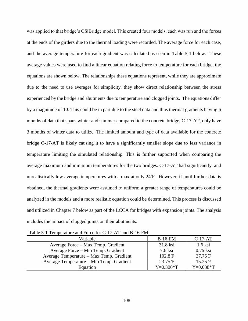
108
was applied to that bridge’s CSiBridge model. This created four models, each was run and the forces
at the ends of the girders due to the thermal loading were recorded. The average force for each case,
and the average temperature for each gradient was calculated as seen in Table 5-1 below. These
average values were used to find a linear equation relating force to temperature for each bridge, the
equations are shown below. The relationships these equations represent, while they are approximate
due to the need to use averages for simplicity, they show direct relationship between the stress
experienced by the bridge and abutments due to temperature and clogged joints. The equations differ
by a magnitude of 10. This could be in part due to the steel data and thus thermal gradients having 6
months of data that spans winter and summer compared to the concrete bridge, C-17-AT, only have
3 months of winter data to utilize. The limited amount and type of data available for the concrete
bridge C-17-AT is likely causing it to have a significantly smaller slope due to less variance in
temperature limiting the simulated relationship. This is further supported when comparing the
average maximum and minimum temperatures for the two bridges. C-17-AT had significantly, and
unrealistically low average temperatures with a max at only 24 ̊F. However, if until further data is
obtained, the thermal gradients were assumed to uniform a greater range of temperatures could be
analyzed in the models and a more realistic equation could be determined. This process is discussed
and utilized in Chapter 7 below as part of the LCCA for bridges with expansion joints. The analysis
includes the impact of clogged joints on their abutments.
Table 5-1 Temperature and Force for C-17-AT and B-16-FM
Variable B-16-FM C-17-AT
Average Force – Max Temp. Gradient 31.8 ksi 1.6 ksi
Average Force – Min Temp. Gradient 7.6 ksi 0.75 ksi
Average Temperature – Max Temp. Gradient 102.8 ̊F 37.75 ̊F
Average Temperature – Min Temp. Gradient 23.75 ̊F 15.25 ̊F
Equation Y=0.306*T Y=0.038*T

109
5.5 Summary and Preliminary Conclusions
The impact of temperature, thermal gradients, and overall shifts in temperature due to
changing seasons have a significant effect on bridge expansion joints in Colorado. The potential for
0.01 in of movement and 0.5 ksi in stress increase on concrete bridges regularly and 0.5 in
movement and 5 ksi stress on steel bridges regularly is not negligible. Furthermore, this preliminary
data on the concrete bridge C-17-AT only accounts for mid -inter and does not account for the
hottest or coldest days of the year which can cause the greatest movement in the expansion joint.
This fact should be kept in mind when considering these preliminary findings and their application.
However, these limited observations do imply that if CDOT is interested in removing an expansion
joint, the bridge superstructure and retrofit option would need to support the movement of the bridge
at the abutment and the potential for abutment stresses due to movement. These displacements do
not appear so great as to require the use of an expansion joint. On the other hand, more data at
different times of the year is needed for a more definite recommendation.
Removing the joint would eliminate the concentrated stresses which could prevent possible
fatigue cracking at joints. This would not eliminate the stresses introduced at the abutment and could
introduce more. In the event of joint removal, the abutments would need to be analyzed and
reinforced to support these stresses due to the temperature gradients and thermal contraction and
expansion. Nonetheless, the impact and potential benefits of constructing a bridge without deck joints
or bearings or eliminating all deck joints and bearings by retrofitting an existing bridge is
significant. The behaviors of interest and parameters influencing them are numerous and vary for
new construction and existing bridges. These parameters and costs are analyzed further in Chapter 7.
Additionally, based on the comparison of thermal gradients with standard gradients further research
is needed to determine a more accurate standard for temperature gradient prediction. This would not
only help predict stresses around a joint due to thermal gradients, but also benefit abutment design

110
for continuous or retrofitted bridges. All of which could potentially lead to a more economical and
safe design. Finally, more scientifically verified information on the response of reinforced concrete
and steel bridges and development of well-understood replacement connections would assist in
furthering the concept of deck joint replacement and, therefore, decrease maintenance costs and
increase the durability of bridges’ superstructures.

111
CHAPTER 6
PARAMETRIC STUDY FOR C-17-AT
6.1 Introduction
Below describes the numerical model and parametric study performed using the CSiBridge
three-dimensional numerical model of C-17-AT, which was validated using the control load test
discussed in Chapter 4. The objectives of the parametric study were to consider the different code
based thermal gradients and the effects of these thermal loads on the joint and bridge performance.
The behavior of the bridge under different amounts of joint clogging while under thermal loads was
also examined. Different joint elimination scenarios were also examined to provide DOT engineers
with the implications of different joint removal alternatives. Three joint removing connections, three
thermal load scenarios, and three joint clogging scenarios were analyzed.
6.2 CSiBridge Finite Element Numerical Model
The finite element software chosen was CSiBridge which is used by many practicing engineers.
The software was created by the same developers as SAP2000 and was chosen by CDOT due to its
heavy presence in private consulting.
The finite element model was built using thin shell elements for the girders and slab, as seen
in Figure 6-1. The thin shell elements were assigned dimensions and area section properties to match
the properties of bridge C-17-AT. Rebar was included for both compressive and tensile
reinforcement in the girders and for two-way slab action in the concrete deck. For concrete properties,
the compressive strength of 4000 psi concrete was defined along with a modulus of elasticity of 3604

112
ksi. The shell elements were meshed at six inch intervals to provide uniform response and minimize
computational time.
Composite action was obtained using short frame elements connecting the girders to the slab,
these short frame elements were assigned Grade 50 steel properties with a modulus of elasticity of
29000ksi. These elements represented the shear studs used in traditional reinforced concrete
construction to connect girders to slabs. The stiff links are shown as blue lines connecting the node
on the girder to a node on the slab in Figure 6-2 below. These stiff link shear studs were sized so that
their cross-sectional area matched that of the shear connectors detailed in the construction documents
in Appendix A.
Figure 6-1 C-17-AT Finite Element Model.
Figure 6-2 C-17-AT Finite Element Model Ties Between Girder and Slab
Several loading scenarios were analyzed. Self-weight dead loads, point loads, and uniform
loads were applied for the first verification stage. Theoretical calculations were also made using
these same loads and composite beam theory in order to perform the initial verification. The second
verification stage is discussed in Chapter 4 and used a CDOT A-40 truck’s axel loads on the
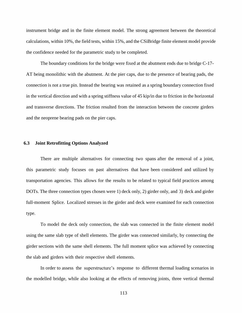
113
instrument bridge and in the finite element model. The strong agreement between the theoretical
calculations, within 10%, the field tests, within 15%, and the CSiBridge finite element model provide
the confidence needed for the parametric study to be completed.
The boundary conditions for the bridge were fixed at the abutment ends due to bridge C-17-
AT being monolithic with the abutment. At the pier caps, due to the presence of bearing pads, the
connection is not a true pin. Instead the bearing was retained as a spring boundary connection fixed
in the vertical direction and with a spring stiffness value of 45 kip/in due to friction in the horizontal
and transverse directions. The friction resulted from the interaction between the concrete girders
and the neoprene bearing pads on the pier caps.
6.3 Joint Retrofitting Options Analyzed
There are multiple alternatives for connecting two spans after the removal of a joint,
this parametric study focuses on past alternatives that have been considered and utilized by
transportation agencies. This allows for the results to be related to typical field practices among
DOTs. The three connection types chosen were 1) deck only, 2) girder only, and 3) deck and girder
full-moment Splice. Localized stresses in the girder and deck were examined for each connection
type.
To model the deck only connection, the slab was connected in the finite element model
using the same slab type of shell elements. The girder was connected similarly, by connecting the
girder sections with the same shell elements. The full moment splice was achieved by connecting
the slab and girders with their respective shell elements.
In order to assess the superstructure’s response to different thermal loading scenarios in
the modelled bridge, while also looking at the effects of removing joints, three vertical thermal

114
distributions were utilized. Two of these distributions had a gradient through the depth of the
bridge while the third had a uniform thermal distribution. The first thermal gradient considered
was adopted from the AASHTO LRFD Bridge Design Specifications and the second thermal
gradient considered was based on the New Zealand bridge design code. This New Zealand code
was selected because a previous study conducted by French et al. (2013) showed reasonable
agreement between this fifth order gradient curve and the field-measured thermal loading on the
bridge studied. Finally, a uniformly distributed temperature change of 50oF was applied. The
uniform temperature distribution entailed an increase of 50o
F, which was applied to the entire
cross-section along the length of the spans in order to determine how thermal stress from a
uniform thermal gradient compares to varying vertical thermal gradients. An increase of 50o
F was
chosen because all bridges in Colorado experience this temperature change over the course of one
year. The AASHTO and New Zealand thermal gradients are shown in Figure 6-3 below.
The temperatures were applied to the bridge model using a piece-wise thermal gradient
method modelled after an example entitled Temperature Changes and Fabrication Errors in the
textbook Matix Analysis of Structures by Aslam Kassimali (2012). The piece-wise approximation
divides the girder and slab into elements and each element is assigned a single temperature based
on the equivalent piece-wise distribution of the thermal gradient. For the model of C-17-AT the
bridge’s depth is divided into 5 shell elements including the slab thickness. The piece-wise
approximations for the AASHTO, New Zealand, and Uniform thermal gradients are shown below
in Figure 6-4.

115
Figure 6-3 (a) AASHTO Thermal Gradient, (b) New Zealand Thermal Gradient.
(a)
(b)

116
Figure 6-4 Piece-wise Approximation: (a) AASHTO Thermal Gradient, (b) New
Zealand Thermal Gradient, (c) Uniform Gradient
(a)
(b)
(c)

117
6.4 Joint Clogging Stiffness Considered
Past research has identified that joints are often clogged with debris soon after being placed into
service (Chen, 2008). In order to model this clogging in CSi Bridge, axial stiffness coefficients were
assigned to links connecting the slabs across the joints. These axial stiffness coefficients were calculated
based on the moduli of elasticity of soil types that commonly clog joints, sand and gravel. Stiffness values
(k) are typically calculated as EA/L, where E is the modulus of elasticity, A is the area, and L is the length
of the element.
The soil volume clogging the joint is the structural element considered for the axial stiffness.
Gravel as a typical modulus of elasticity of 22 ksi (150 MPa ) and sand has a modulus of elasticity of 7
ksi (50 MPa ) (Briaud, 2013). The length of the clogging debris was taken as the joint opening which was
0.125 inches (L) as measured in the field. Axial stiffness was determined for each soil type and a blend.
The stiffness placed evenly across the joint by placing links every six inches in the transvers direction.
This assumes that the joint is evenly clogged along its length, and consequently assumes no torsional
effects. The axial stiffness coefficients were taken as 30 kip/in for gravel filled joints, and 10 kip/in (~1751
kN/m) for sand filled joints, and 20 kip/in (~3502 kN/m) for a joint that is clogged with a mixture of
gravel and sand. The same methodology was used in analyzing the steel bridge as outlined in Rager (2016).
6.5 Parametric Analysis Matrix
The effects of the different combinations of connection type, clogging material, and thermal
gradients on local and global performance were examined using a parametric study matrix shown in
Figure 6-5 below. The two types of joint alterations, clogging and connection type, were analyzed with

118
each of the three thermal gradients. All analysis were conducted using the finite element model of C-17-
AT and the results are discussed below in Section 6.6.
Thermal
Gradients
Stiffness of Clogging Links Across
Joints
Connection Retrofit
10 kip/in 20 kip/in 30 kip/in Deck Only Deck and Girder
AASHTO x x x x x
New Zealand x x x x x
Uniform
(+50˚F)
x x x x x
Figure 6-5 Parametric Study Matrix
6.6 Analysis Results and Implications
The results and implications of the parametric study analysis are divided into two sections: those
associated with clogged joints and those associated with the retrofit connection types. The results from
the clogged joints are presented as line graphs because the stiffness assigned to the two-joint links are
continuous quantitative variables. However, the retrofit connection types are discreet qualitative variables
and are therefore presented as bar charts for comparison.
In order to analyze the different connection types and clogged joint stiffness and their effect on
global and local bridge behavior three different load scenarios were examined: thermal gradient load only,
truck load only, and thermal gradient and truck loads combined. The truck load used was an AASHTO
HS2044 truck as shown in Figure 6-6 below.

119
Figure 6-6 AASHTO HS20-44 Truck (Precast/Prestressed Concrete Institute, 2003)
The location of the truck was determined by performing an influence line analysis to find the
location that produced the maximum moment demand. This location was found to be where the front axle
is over the bearing near the beginning of the span and the back two axles are placed 14 feet apart (V=14
feet). In the remainder of the chapter, truck loading refers to this location of the AASHTO HS20-44 truck
on the bridge.
6.6.1 Clogged Joint Results and Implications
The effects of clogged joints in the parametric study on the bridge as analyzed using the truck
loading, thermal gradients, and values for link stiffness (k = 10 kip/in, 20 kip/in, 30 kip/in) described
above. The analysis was performed considering only the thermal and truck loads, the dead load due to
self-weight of the bridge was neglected.
First, the maximum stress in the bottom of the girder at the ends and at the mid-span due only to
each of the three thermal gradients was determined for each of the three link stiffness values. Figure 6-7

120
and Figure 6-8 show these results for the girder ends and girder mid-span. The model experienced a
maximum compressive stress of 0.217 ksi in the girders at mid-span, with a 10 kip/in link stiffness and
under the AASHTO thermal gradient load. The maximum tensile stress in the bottom of the girders was
0.026 ksi in the girders at mid-span, with a link stiffness of 30 kip/in and under the Uniform thermal
gradient load.
The maximum loads experienced in the girders due to all thermal gradient loads occur at mid-
span. At the bottom ends of girders the AASHTO thermal gradient is the most conservative with
compressive stress at around zero due to no temp load applied at the base of this gradient. On the other
hand, the AASHTO thermal load gives the largest compressive stresses at the girder bottoms at mid-span
due to the larger moment induced by the gradient. New Zealand is the middle loading gradient with the
Uniform thermal load behaving conversely to the AASHTO gradient giving the largest compressive stress
at the bottom of girder ends and the least at mid-span.
Figure 6-7 Maximum Stress in Bottom of Girder at End
-0.07
-0.05
-0.03
-0.01
0.01
0 5 10 15 20 25 30 35
Stre
ss (
ksi)
Stiffness (kip/in)
AASHTO New Zealand Uniform

121
Figure 6-8 Maximum Stress in Bottom of Girder at Mid-span
The maximum in the top of the girder was also analyzed at both mid-span and at the ends due to
each of the thermal gradients for each of the link stiffness values, shown in Figure 6-9 and Figure 6-10
below. The maximum tensile stress for each link stiffness value was produced due to the AASHTO
thermal gradient load induced moment at mid-span in the top of the girders. This is expected since
AASHTO had the highest temperature load difference between top and bottom of the girder. Whereas the
maximum tensile stress was at each of the link stiffness values was produced by the Uniform thermal
gradient load in the girder at mid-span. Overall, comparing the two standard thermal gradients, AASHTO
appears to have the more conservative gradient due to the larger difference in temp between top and
bottom despite New Zealand applying a greater maximum temperature at the top.
In all four figures the clogged joints, symbolized by the link stiffness values, do not show a
significant impact on the global or local demand on the bridge superstructure. Both the stresses at the top
and bottom of the girders showed relatively small changes in compressive and tensile stress under each
thermal gradient load as the stiffness increased. The maximum stress range on the girders for the different
-0.27
-0.22
-0.17
-0.12
-0.07
-0.02
0.03
0 5 10 15 20 25 30 35
Stre
ss (
ksi)
Stiffness (kip/in)
AASHTO New Zealand Uniform

122
stiffness values were 0.02, 0.05, and 0.06 ksi for AASHTO, New Zealand, and Uniform thermal gradients
respectively, all less than 0.1 ksi difference.
Figure 6-9 Maximum Stress in Top of Girder at Mid-span
Figure 6-10 Maximum Stress in Top of Girder at the Ends
With the clogging stiffness established as not having significant impacts on the bridges behavior
a truck load was added to the analysis. The HS20-44 truck was examined first with only the truck and
second combined with the thermal gradient loads. Figure 6-11 below show the results of the model with
-0.15
-0.05
0.05
0.15
0.25
0.35
0 5 10 15 20 25 30 35
Stre
ss (
ksi)
Stiffness (kip/in)
AASHTO New Zealand Uniform
-0.15
-0.05
0.05
0.15
0.25
0.35
0 5 10 15 20 25 30 35
Stre
ss (
ksi)
Stiffness (kip/in)
AASHTO New Zealand Uniform

123
the truck loading and clogging stiffness. The truck load’s moment demand on the bridge decreases slightly
due to the clogged joints modeled by the link stiffness values because the simulated clogged joints hold
the concrete in a negative moment region. Consequently, some moment is transferred in this negative
moment region and the positive moment region’s moment demand will decrease slightly unlike in an
unclogged joint. This overall decrease is only about 0.0257 ksi which is only 0.4% of the moment demand
with an unclogged joint and as such is insignificant, reinforcing the insignificance of the stiffness of the
clogged joint.
Figure 6-11 Stress Demand in Bottom of Girder at Mid-span due to Moment resulting
from the Truck Load
Next, the analysis of the thermal and truck loading combined was conducted and the results are
shown below in Figure 6-12. The Uniform thermal gradient showed the most obvious change between
just the thermal load and the thermal load and truck load, with an increase of about 0.6 ksi. This is likely
due to the Uniform gradient having almost no stress at this location by itself and thus was the addition of
the truck load was close to total. The New Zealand and AASHTO gradient moved from compression to
tension with an average stress change of about 0.6 ksi as well, moving from about -0.22 ksi to 0.38 ksi.
Indicating that the truck load counteracts the thermal load on the bridge.
0.55
0.57
0.59
0.61
0.63
0.65
0 10 20 30 40
Stre
ss (
ksi)
Stiffness (kip/in)
Truck

124
Additionally, similar to when examining the thermal gradient loads only, the combined loads
showed negligible changes in stress relative to the increase in clogged link stiffness. The maximum stress
range on the girders for the different stiffness values were 0.012, 0.026, and 0.03 ksi for AASHTO, New
Zealand, and Uniform thermal gradients respectively.
Figure 6-12 Moment Demand Due to Thermal and Truck Load in Bottom of Girder at
Mid-span
6.6.2 Joint Retrofit Connection Results and Implications
First, the maximum stress at the bottom of the girders near the bearings due only to the thermal
gradients was determined for each connection type. Figure 6-13 below shows these stress values. The
stresses induced by the AASHTO recommend thermal gradient is a lower tensile stress when compared
to the New Zealand Gradient, whereas the Uniform thermal gradient gives the largest compressive stresses.
This is to be expected because the uniform thermal gradient is a uniform temperature increase of 50˚F
throughout the depth of the structure. Therefore, the temperature load at the bottom of the girder for the
uniform gradient of 50˚F is significantly larger than the 20.82˚F and 0˚F for the New Zealand and
AASHTO recommended thermal gradients respectively. This larger temperature load will cause greater
thermal expansion of the concrete and consequently greater compressive stresses. Conversely, the
AASHTO recommend thermal gradient has the lowest temperature load at the bottom of the girder and
0.35
0.45
0.55
0.65
0 10 20 30 40
Stre
ss (k
si)
Stiffness (kip/in)
AASHTO New Zealand Uniform

125
therefore it is reasonable that it should produce lower compressive stresses when the bridge is only
exposed the thermal loads with the two retrofit options. The Deck Only connection produces lower
stresses than the Full Moment Splice connection for all three thermal gradients. The significant difference
is likely due to the boundary conditions on the bridge; the abutment connections for the superstructure
are fixed conditions. Thus, when the deck is connected the joints are now transferring a little of the
moment capacity contained in the fixed ends through to the center span. However, when the deck and
girders are connected in a Full Moment Splice that entire moment can be carried throughout the length of
the bridge, across all spans, significantly increasing the moment capacity. This allows a negative moment
region across the supports and increases the moment capacity and thus the stress in the girders. For the
AASHTO and New Zealand thermal gradients, the Full Moment Splice increases the tensile stress
significantly. This is likely due to the lower temperature loads at the bottom of the girder when compared
to the top. The difference, of 30-40˚F, creates significantly greater compression in the top versus the
bottom and induces a moment that the Full Moment Splice allows to be carried, increasing the stress.
Figure 6-13 Maximum Stress at Bottom of Girder due to Thermal Gradients Only
-0.4
-0.2
0
0.2
0.4
0.6
0.8
1
1.2
1.4
1.6
Deck Only Full Moment Splice
Stre
ss (k
si)
Connection Types
AASHTO
New Zealand
Uniform

126
In order to fully evaluate a potential increase in the span’s moment capacity for the two retrofit
connection types considered, the analysis was performed for only the truck load with each of the
connection types. The stress values due to the truck loading are shown below in Figure 6-14. The
maximum stress at the bottom of the girders near the bearings was measured to gauge the moment demand
for each connection type. When the Deck Only connection was examined the truck load induced a tensile
stress in the girders of 0.06 ksi, whereas when the Full Moment Splice was examined the truck load
induced a greater compressive stress of 0.46 ksi. This change from tensile to compressive stress indicates
an increase in moment capacity of the superstructure, corresponding to a 75 % decrease in moment
demand.
Figure 6-14 Maximum Stress at Bottom of Girder due to Truck Loading Only
Once thermal gradient loads and truck loading scenarios were analyzed separately, analysis was
completed for combined thermal and truck loading for both connection types. The stress at the bottom of
the girders near the bearings due to both loads are shown in Figure 6-15 below. Comparing Figure 6-13
and Figure 6-14 with Figure 6-15 it is evident that under the deck only connection the stresses increased
-0.6
-0.5
-0.4
-0.3
-0.2
-0.1
0
0.1
Deck Only Full Moment Splice
Stre
ss (k
si)
Connection Types

127
in tension. Under the uniform thermal gradient and deck only retrofit connection, the truck load caused
the stress to switch from compressive to tensile. On the other hand, the truck load in the full moment
splice connection decreased the tensile stress under the AASHTO and New Zealand thermal gradients,
and increased the compressive stress when the uniform thermal gradient was applied. This change in
stress illustrates how the connection type for joint retrofitting influences global moment demand on the
bridge when considering thermal gradients. The truck load counteracts the thermal loads once again, and
the full moment splice increases the bridge’s moment capacity significantly compared to the deck only
connection.
Figure 6-15 Maximum Stress at Bottom of Girder due to Thermal Gradients and
Truck Load Combined
6.7 Conclusion
These parametric study results illustrate the differences between the thermal gradients and joint
retrofit connection types considered. The thermal gradients when subjected to different joint clogging
stiffness values showed relatively little change in stress as the stiffness increased. At mid-span the
-0.8
-0.6
-0.4
-0.2
0
0.2
0.4
0.6
0.8
1
Deck Only Full Moment Splice
Stre
ss (k
si)
Connection Types
AASHTO
New Zealand
Uniform

128
AASHTO thermal gradient showed the greatest stresses, while at the girder ends the Uniform thermal
load showed the greatest stress. Applying a standard truck load to the bridge counteracted the stresses and
moments induced by the thermal loads.
When applied to the different connection types the thermal gradients and truck load’s impact on
the bridge’s moment capacity was examined. The New Zealand thermal gradient showed the greatest
difference in stress load for the two different connection types. This can be connected to the fact that the
New Zealand thermal gradient has the greatest temperature at the top of the gradient creating a difference
of about 40˚F between top and bottom, and inducing significant expansion at the top with the potential
for moment transfer when fully connected. A decrease in moment demand was observed when the Full
Moment Splice connection was used under only truck loading. However, the moment capacity and
demand increased when the truck load was combined with the AASHTO and New Zealand thermal
gradients and a Full Moment Splice was utilized. This increase in demand is influenced by the fixed ends
of the bridge at the abutments which allow for moment transfer throughout the length of the bridge when
a Full Moment Splice connection is used. With the full moment splice connection giving the greatest
increase in moment capacity the full moment splice will be assumed for the retrofit to continuous analysis
in the LCCA in Chapter 8.

129
CHAPTER 7
PARAMETRIC STUDY FOR B-16-FM
7.1 Introduction
One of the primary objectives of this study was to establish a finite element model to assess
thermal movements, thermal stresses, and joint removal retrofit options. The developed design and
assessment procedures were developed with the intent to be used in industry for eliminating bridge joints.
Therefore, choosing a finite element software that is widely used by practicing engineers is vital to correct
implementation of the developed procedure. CSi Bridge software (same developers as SAP2000) was
chosen by CDOT due to its prevalence of use in private practice. This chapter focuses on the model for
the steel bridge; B-16-FM. Theoretical calculations were performed using composite beam theory in order
to verify the finite element model.
Multiple loading scenarios were considered. Dead loads due to self-weight, uniform loads, and
point loads were considered first during the verification process. Then, live loads due to AASHTO HS20-
44 loading and a CDOT A-40 snooper truck were examined. Agreement between the CSi Bridge model,
the theoretical calculation, and field measurements was found to be very good. The strong validation of
the finite element models solidified confidence in the results of the parametric study discussed in Chapter
6.

130
7.2 B-16-FM: Steel Plate Girder Bridge with Concrete Slab
Geometric and structural properties specific to B-16-FM, and the modeling techniques, are
discussed in this section. The structural information and dimensions were obtained from the construction
documents provided by CDOT. The bridge is described in Section 3.2 with photos from the site. Steel
plate girders support three spans with a length of 75 ft (~23 m) each and one shorter approach span (44 ft
(~13.4 m)) at the end of the bridge is supported by concrete girders. The steel span’s superstructure
consists of three plate girders that are spaced at 10 ft (~3 m) on center in the transverse direction.
The top and bottom flange thickness of the plate girders varies along the length. The flanges
nearest to the vertical supports are 5/8” thick. The thickness of the flanges increases to 1 ¼” (31.75 mm)
after a distance of 11 ft (~3.35 m) from the supports is reached. Finally, for the central 32 ft (~9.75 m) of
the girders, the flanges are 1 ¾” (44.45 mm) thick. Figure 7-1 shows the layout of flange variance in one
girder that is typical for all three steel spans.
Figure 7-1. Plate Girders in Construction Documents for Bridge B-16-FM (Courtesy CDOT)
Intermediate stiffeners are located along the length of the plate girders and bearing stiffeners are
located near the supports. The web is 5/16” inches thick and 44” in height. The diaphragms between
girders were excluded from the model. The main function of the diaphragms is to tie the girders together
during construction so their absence in the finite element model is trivial. In the case of bridge skewedness

131
or curvature, then torsional stresses could develop, which would require that the diaphragms are kept in
place. Since this bridge does not possess any skew, curvature (no torsion-induced loading), the
diaphragms are excluded from the finite element model. Figure 7-2 shows the extruded view of the plate
girders with the intermediate and bearing stiffeners. The slab is excluded from this view to better show
the girders.
Figure 7-2. Plate Girders for Bridge B-16-FM
The slab was modeled considering the super-elevation described on the construction documents.
The high point of the slab is along the centerline of the roadway and a slope of 0.015 ft/ft downwards
exists on each side until the centerline of the outside girders. Then the slab ceases to change elevation.
This results in an elevation at the edge of the deck that is 2.4 inches lower than at the centerline. Figure
7-3 shows the slab geometry in the construction documents and Figure 7-4 shows the slab geometry in
the finite element model.

132
Figure 7-3. Slab Geometry described in the Construction Documents
(Courtesy CDOT)
Figure 7-4. Finite Element Model Illustration of super-elevation described in the Construction
Documents
The bridge’s bearings transfer the superstructure load to the pier caps. The bearings for the steel
bridge disallow translation and allow rotation at the end of each girder. Therefore, the supports are
modeled as pin connections that prevent translation in all directions and allow rotation about all axes. The
boundary conditions are further discussed in Section 4.3.5.
A few more views of the full-scale bridge model are shown in the following figures. The different
materials are represented by different colors, cyan and red for the steel and concrete, respectively. Figure
7-5 shows an extruded view of the superstructure. Figure 7-6 shows all spans in the superstructure.

133
Figure 7-5. Extruded View of B-16-FM Superstructure
Figure 7-6. Alternative view of B-16-FM Bridge Model (unstressed, unloaded state)
7.3 CSi Bridge Model Methodology
A three-dimensional model was used to capture both the localized behavior at the joints and the
global response to thermal loading with great accuracy. To build the three-dimensional model, shell and
frame elements were used in CSi Bridge to represent various bridge elements. The model was used to
examine the effects of gravity loading, dynamic loading, thermal loading (both uniform temperature
changes and non-uniform gradients), deck joint performance, on the behavior of the bridge. After
validating the model’s responses, the model was used to perform the parametric study discussed in
Chapter 6.
Concrete Slab
Pinned Supports Plate Girders
75 ft 75 ft75 ft
44 ft

134
7.3.1 Shell and Frame Elements
Shell elements were used for the majority of the structural elements in the bridge. Flange, web,
intermediate stiffeners, and bearing stiffeners were modeled individually with properties of Grade 50 steel
and with the thickness as described in the construction documents. The built up plate girder was connected
to the slab with shear studs composed of an appropriately sized, steel frame sections. Finer mesh sizes
were utilized in areas of interest near the joints and for more detailed thermal gradients.
7.3.2 Composite Behavior
Short, frame elements were used to model shear studs between the top of the girders and the slab
component of the bridge. The total cross-sectional area of the shear studs was the same as that provided
by the shear connectors described in the construction documents. In both the actual bridge and the CSi
Bridge model, the concentration of the shear stud elements was greater near the supports to accommodate
greater shear transfer in regions of high shear demand. The spacing of the studs in the model differed
slightly from those on the actual bridge due to node locations in the model that accommodated the
changing of the flange thicknesses along the length of the span.
The frame elements used to model shear studs were connected from a node of the girder to a node
of the slab that was directly above. The frame elements were given a modulus of elasticity of 29,000 ksi,
typical of steel, and were assigned a yield strength of Grade 50 steel. However, the shear studs are not
anticipated to yield in this study and all behavior is considered linear-elastic. The top of the web section
is connected to the centroid of the slab section with these frame elements. The frame elements were
assessed for proper behavior and shear transfer. Figure 7-11 shows the shear load in the frame elements
for one girder under self-weight. Shear lag behavior is evident directly above the supports. The maximum
shear force is observed near the supports. The minimum shear force is observed at mid-span and the shear
load switches direction at mid-span. This behavior is reasonable and expected.

135
7.3.3 Thermal Analysis
Shell and frame elements were assigned temperatures in degrees Fahrenheit to simulate thermal
loading scenarios. Various temperature loads were assigned to flanges, web, and slab elements to simulate
vertical temperature gradients and uniform temperature changes. The thermal gradients considered were
put into the model by determining an equivalent piece-wise distribution such that individual shell
elements could be assigned one temperature. Prior to using this method in the bridge model, validation
analysis was conducted to ensure that this procedure yielded reasonable results. The number of shell
elements in the depth of the plate girder varied between five and ten elements, depending on proximity to
the joint. Further information on this validation is discussion in Section 4.4: Model Validation.
7.3.4 Boundary Conditions
A pinned boundary condition refers to a joint restraint at that allows free rotation with respect to
the x-, y-, and z- axes, but does not allow translation in the x-, y-, or z- axes. A fixed boundary condition
refers to a joint restraint that does not allow rotation or translation in any direction or axis. The bearings
on the steel bridge display behavior that is very close to that of pinned joints. Therefore, the supports at
the ends of the girders were modeled in this manner.
Due to the shell element configuration of the model, many nodes were available upon which the
pinned boundary conditions can be imposed. The boundary conditions had to be applied to multiple nodes
in the model to achieve pinned support behavior. Figure 7-7 below shows an end view of one of the
girders. Each node with a triangle beneath it has had the translation restrained but not the rotation.
Different configurations of joint restraints were considered without significant effects on the global
performance of the bridge. However, the boundary configuration chosen, and indicated in the figure, was
that which displayed the greatest similarity to the expected localized stress distributions at a pinned joint
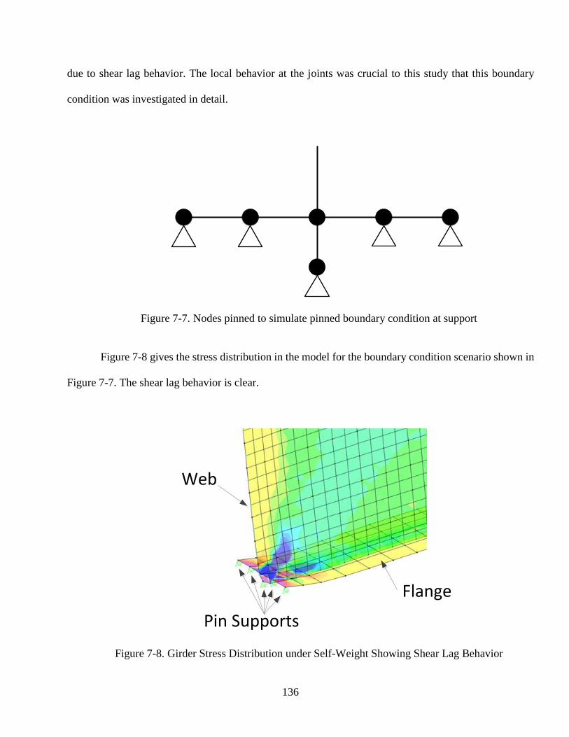
136
due to shear lag behavior. The local behavior at the joints was crucial to this study that this boundary
condition was investigated in detail.
Figure 7-7. Nodes pinned to simulate pinned boundary condition at support
Figure 7-8 gives the stress distribution in the model for the boundary condition scenario shown in
Figure 7-7. The shear lag behavior is clear.
Figure 7-8. Girder Stress Distribution under Self-Weight Showing Shear Lag Behavior
Flange
Web
Pin Supports

137
7.4 Joint-Removing Connection Types Considered
While it is recognized that there are numerous alternatives for connecting two spans following the
removal of a joint, this parametric study focus on previous alternatives that are considered common
among transportation agencies. This is to allow for the results of this study to be related to typical field
practices. Specifically, connection types used in the two-dimensional study performed by Tsaistas and
Boardman (described in Chapter 2) were examined with the three-dimensional model developed for this
project. This provided an opportunity to compare results and draw conclusions about how necessary a
three-dimensional model is to assess joint removal and thermal loading. The four connection types chosen
were 1) deck only, 2) deck and top flange, 3) deck, top flange, and bottom flange, and 4) full-moment
splice. Localized stresses and alterations in bending behavior were assessed for each connection type.
To model the deck only connection, the slab was connected in the finite element model using the
same types of shell elements. Flanges were connected similarly, by connecting the steel sections with the
same shell elements. The full moment splice was achieved by connecting the slab, web, and both flanges
with their respective shell elements. The bearing was retained as a pinned boundary condition (allowing
rotation, but no translation).
7.5 Thermal Gradients Considered
To assess the effect of removing joints on the superstructure’s response to different thermal
loading scenarios in the modeled bridge, three vertical thermal distributions were utilized. Two of the
distributions had a gradient while the third had a uniform thermal distribution. The first thermal gradient
considered was adopted from the AASHTO LRFD Bridge Design Specifications and the second thermal
gradient considered was based on the New Zealand bridge design code. This New Zealand code was

138
selected because a previous study conducted by French et al. (2013) (see Chapter 2) showed reasonable
agreement between this fifth order gradient curve and the field-measured thermal loading on the bridge.
Lastly, a uniformly distributed temperature change of 50oFwas applied. Both the AASHTO and New
Zealand distributions are described in details in Section 2.8.4. The uniform temperature distribution
entailed an increase of 50oF, which was applied to the entire cross-section along the length of the spans
in order to determine how thermal stress and behavior from a uniform thermal gradient compares to
varying vertical thermal gradients. An increase of 50oF was chosen because all bridges in Colorado
experience this temperature change over the course of one year.
7.6 Connection Link Stiffness Considered
Previous research described in Chapter 2 has identified that joints are commonly clogged with
debris quickly after they are put into service. To model this in CSi Bridge, links were used and axial
stiffness coefficients were assigned to the links to simulate a bridge joint clogged with debris. The axial
stiffness coefficients were assigned based on the moduli of elasticity of soils that are known to clog these
joints: sand and gravel. Typically, stiffness values (commonly assigned the variable ‘k’) are found as
EA/L, where E represents the modulus of elasticity, A represents the cross-sectional area, and L represents
the length of the element.
To calculate the axial stiffness of the links to reasonably represent the clogged joint, the structural
element considered is the soil volume blocking the joint. Common moduli of elasticity for gravel and
sand are ~22 ksi (150 MPa) and ~7 ksi (50 MPa), respectively (Briaud, 2013). The length of the debris
clog that is being modeled as an additional structural element is taken as the joint opening as described in
the construction documents (L=0.625 in). The area is found by multiplying the transverse dimension of
the bridge by the height of the debris that is causing the clog. The height of the clogged debris was

139
assumed to be 3 inches (76.2 m). This depth was chosen because 3 inches is a common depth of
compression seals that are used at the expansion joints. Using these assumptions, a total stiffness of the
debris clogging the joint is determined. Then, the stiffness is distributed evenly across the joint in the
model with a link every foot in the transverse direction. This method assumed that the joint is evenly
clogged, and thus there are no resulting torsional effects. Using this method, stiffness coefficients of 30
kip/in for a totally gravel filled joint and 10 kip/in for a totally sand filled joint were selected. Additionally,
a stiffness of 20 kip/in was selected for a joint that is clogged with a mixture of sand and gravel. These
stiffness values were implemented in the parametric study.
7.7 Parametric Study Matrix and Overview
In order to examine the effects of different combinations of connection types, clogged joints, and
vertical thermal gradient, on local behavior and global performance, a parametric study matrix was
developed and is shown in Figure 7-9 below. Two categories of joint alterations (connection types and
clogged joints) are analyzed with each type of thermal gradient. All analysis took place in the finite
element model described in Chapter 4 and Chapter 5. Results and conclusions drawn are discussed in
Section 6.6.
10 kip/in 20 kip/in 30 kip/in Deck OnlyDeck and Top
Flange
Deck, Top Flange,
and Bottom
Flange
Full Moment
Connection
AASHTO
New Zealand
Uniform (+50oF)
Stiffness of Deck Clogging Links Between Spans
Te
mp
era
ture
Gra
die
nt
Connection Types
Figure 7-9. Parametric Study Matrix

140
7.8 Results
The results of the parametric study are subdivided into two sections: results associated with
clogged joints and results associated with various connection types. The numerical results from the
analysis of different connection types are shown in bar charts because the connection types are discreet,
qualitative variables. However, the stiffness assigned to the two-joint links are quantitative, continuous
variables and the results from these analyses are presented in line graphs.
To analyze the effect that different connection types and clogged joints had upon the global
performance and local behavior of the bridge, three different loading scenarios were considered: 1)
temperature gradient load only, 2) truck loading only, and 3) temperature gradient loading combined with
truck loading. An AASHTO HS20-44 truck was used for the truck loading and is shown in Figure 7-10
below.
Figure 7-10. AASHTO HS20-44 Truck (Precast/Prestressed Concrete Institute, 2003)
An influence line analysis was conducted to determine the location of the truck that resulted in the
maximum moment demand on the bridge spans. This location was determined to be when the font axel

141
was at the over the bearing, near the beginning of the span and the last two axels were placed 14 feet from
one another (when V = 14 feet in Figure 7-10 above). For the remainder of the chapter, truck loading
refers to this AASHTO HS20-44 in this position on the superstructure.
7.8.1 Effect of Clogged Joints
Examination of the influence of clogged joints in the parametric study was conducted in a similar
manner as the examination of the influence of connection type. The location of the truck loading was not
changed. However, since the value of stiffness of the links is a continuous variable, line graphs instead of
bar charts are used to present the results of the study. Three values for link stiffness (k = 10 kip/in, 20
kip/in, and 30 kip/in) are examined with the thermal gradients described above. Local behavior and global
performance were evaluated.
First, the compressive stress at the bottom of the girders near the bearings due to only temperature
gradient was determined for each vertical gradient option for different 2-joint link stiffness options. Figure
7-11 below shows the results of this analysis. The model exhibited the maximum compressive stress,
60.29 ksi, when the uniform temperature increase of 50oF is applied and a link stiffness of 30 kip/in is
considered. Of the clogged joint stresses (k > 0), the minimum compressive stress, 26.91, was exhibited
in the model when the AASTHO thermal gradient is applied with a link stiffness of 10 kip/in. Though the
stresses shown in the figure exceed the yield stress, the analysis was conducted considering only the
thermal loads and the dead load due to the self-weight of the superstructure is neglected. The self-weight
will always be present on the bridge in the field and so the compressive stresses will be less than what is
pictured in the figure that is only representing thermal loads.
The clogged joints (symbolized in the figure below by link stiffness values) do not have a
significant effect on the global demand on the bridge superstructure as seen in Figure 7-11 below. The
compressive stress range on the girders for the different stiffness of links are 0.80 ksi (~5.5 MPa), 0.16

142
ksi (~1.1 MPa), and 0.08 ksi (~0.55 MPa) for New Zealand Gradient, Uniform Temperature Increase, and
AASHTO Gradient, respectively.
Figure 7-11. Compressive Stress at Bottom of Girder
Figure 7-12 shows the results of the analysis shown in Figure 7-11 normalized to the maximum
value of compressive stress in the bottom of the girders for the Uniform Temperature Increase thermal
gradient (60.29 ksi (~416 MPa)). The stress resulting from the gradient described by AASHTO is less
than that of New Zealand by approximately 25%.
0 5 10 15 20 25 300
10
20
30
40
50
60
70
Link Stiffness (kip/in)
Co
mp
ressiv
e S
tre
ss (
ksi)
Uniform Increase
AASHTO Gradient
New Zealand Gradient

143
Figure 7-12. Compressive Stress at Bottom of Girder (Normalized)
Figure 7-13 below shows the local compressive stress in the concrete deck for the different thermal
gradients and link stiffness options. The largest, middle, and smallest, localized compressive stress in the
slab for each link stiffness type was exhibited by the New Zealand, Uniform, and AASHTO gradients,
respectively. This result is in line with what was expected because the temperature values of the thermal
gradient nearest to the top of the concrete deck for New Zealand, Uniform, and AASHTO distributions
were 69.01oF, 50oF, 23.33oF, respectively.
0 5 10 15 20 25 300
0.2
0.4
0.6
0.8
1
Link Stiffness (kip/in)
/
max
Uniform Increase
AASTHO Gradient
New Zealand Gradient
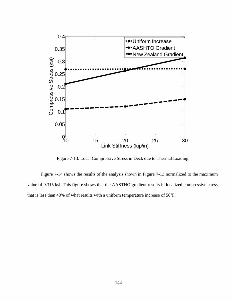
144
Figure 7-13. Local Compressive Stress in Deck due to Thermal Loading
Figure 7-14 shows the results of the analysis shown in Figure 7-13 normalized to the maximum
value of 0.315 ksi. This figure shows that the AASTHO gradient results in localized compressive stress
that is less than 40% of what results with a uniform temperature increase of 50oF.
10 15 20 25 300
0.05
0.1
0.15
0.2
0.25
0.3
0.35
0.4
Link Stiffness (kip/in)
Co
mp
ressiv
e S
tre
ss (
ksi)
Uniform Increase
AASHTO Gradient
New Zealand Gradient

145
Figure 7-14. Local Compressive Stress in Deck due to Thermal Loading (Normalized)
Figure 7-15 shows the results of the model when only a truck load is considered. There is a slight
decrease in moment demand on the bridge due to the clogged joints that are modeled by the links because
they simulate a clogged joint holding the concrete deck together in a negative moment region. Unlike an
unclogged joint then, some moment is transferred in the negative moment region and the moment demand
in the positive moment region decreases slightly. However, this decrease of tensile stress demand under
the truck load is less than 0.1 ksi (~6.9 MPa), which is 0.7%.
10 15 20 25 300.00
0.20
0.40
0.60
0.80
1.00
Link Stiffness (kip/in)
/
max
Uniform Increase
AASHTO Gradient
New Zealand Gradient

146
Figure 7-15. Tensile Stress at Bottom of Girder due to Only Truck Loading
After competition of analysis with separate thermal and truck loading, analysis was conducted
with both loads applied and the results are shown in Figure 7-16 below. For each thermal gradient, the
stresses remained compressive. Uniform Temperature Increase, New Zealand Gradient, and AASHTO
Gradient exhibited the greatest, middle, and least compressive stresses, respectively.
0 10 20 302.0
2.1
2.2
2.3
2.4
2.5
2.0
Link Stiffness (kip/in)
Te
nsile
Str
ess (
ksi)
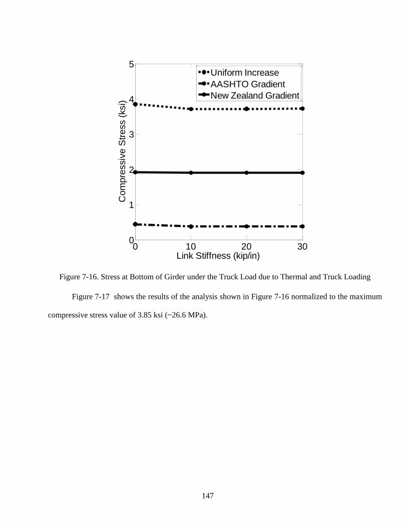
147
Figure 7-16. Stress at Bottom of Girder under the Truck Load due to Thermal and Truck Loading
Figure 7-17 shows the results of the analysis shown in Figure 7-16 normalized to the maximum
compressive stress value of 3.85 ksi (~26.6 MPa).
0 10 20 300
1
2
3
4
5
Link Stiffness (kip/in)
Co
mp
ressiv
e S
tre
ss (
ksi)
Uniform Increase
AASHTO Gradient
New Zealand Gradient
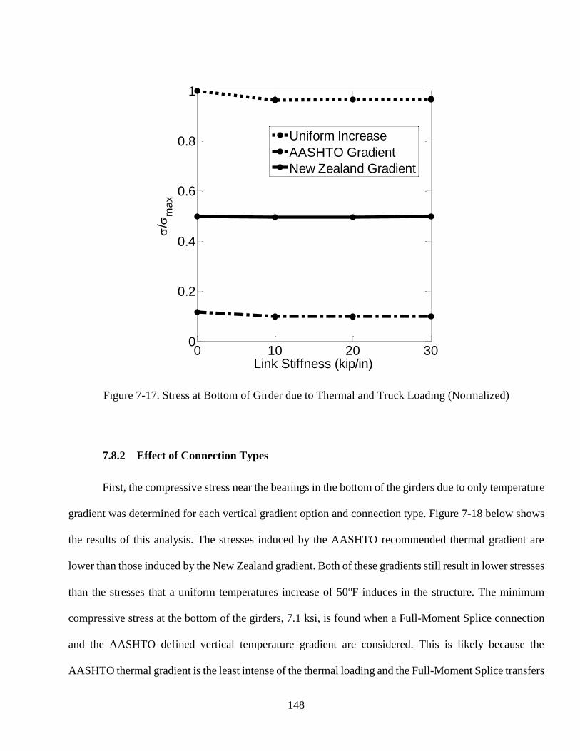
148
Figure 7-17. Stress at Bottom of Girder due to Thermal and Truck Loading (Normalized)
7.8.2 Effect of Connection Types
First, the compressive stress near the bearings in the bottom of the girders due to only temperature
gradient was determined for each vertical gradient option and connection type. Figure 7-18 below shows
the results of this analysis. The stresses induced by the AASHTO recommended thermal gradient are
lower than those induced by the New Zealand gradient. Both of these gradients still result in lower stresses
than the stresses that a uniform temperatures increase of 50oF induces in the structure. The minimum
compressive stress at the bottom of the girders, 7.1 ksi, is found when a Full-Moment Splice connection
and the AASHTO defined vertical temperature gradient are considered. This is likely because the
AASHTO thermal gradient is the least intense of the thermal loading and the Full-Moment Splice transfers
0 10 20 300
0.2
0.4
0.6
0.8
1
Link Stiffness (kip/in)
/
max
Uniform Increase
AASHTO Gradient
New Zealand Gradient

149
moment from one span to the other. The Full-Moment Splice induces a lower neutral axis (the y in the
equation of stress, σ = (M*y)/I, is reduced). Therefore, less stress exists at the most extreme bottom fiber
of a cross-section because the moment demand is lowered at the bottom of the cross-section. Similar to
the clogged joint analysis, the stresses shown in this figure below (and exceed the yield point) are only
depicting the effect of thermal loading and will be lower in the field when the self-weight of the
superstructure is present.
Figure 7-18. Compressive Stress at Bottom of Girder due to Only Thermal Loading
Figure 7-19 shows the results of the analysis conducted in Figure 7-18, but normalized to the
maximum value. The maximum compressive value of stress was 85.0 ksi (~586 MPa) and was found
when the compressive stress due to a uniform temperature increase of 50oF and a Deck, Top, & Bottom
Flange connection was considered.
Deck Only Deck & Top Flange Deck, Top, & Bottom Flange Full Moment Splice0
20
40
60
80
100
Connection Types
Com
pre
ssiv
e S
tress (
ksi)
AASHTO
Uniform
New Zealand

150
Figure 7-19. Compressive Stress at Bottom of Girder due to Only Thermal Loading (Normalized)
To examine the localized behavior at the joints that each thermal gradient and connection type
induces into the structure, the compressive stress at the joint was retrieved from the model results
(considering only thermal loading). Figure 7-20 shows the results of this analysis. The localized
compressive stress induced was the greatest for each thermal gradient when considered with the Deck
Only connection. The localized compressive stress did not significantly decrease, however, with
increasing connectivity at the joint more than attaching one plate girder flange. In other words, the Deck
and Top Flange, Deck, Top, and Bottom Flange, and Full Moment splice connections did not have
progressively lower localized compressive stress.
The largest, middle, and smallest, localized compressive stress in the slab for each connection
type was exhibited by the New Zealand, Uniform, and AASHTO gradients, respectively. This result is in
line with what was expected because the temperature values of the thermal gradient nearest to the top of
the concrete deck for the New Zealand, Uniform, and AASHTO distributions were 69.01oF, 50oF, 23.33oF,
respectively.
Deck Only Deck & Top Flange Deck, Top, & Bottom Flange Full Moment Splice0.0
0.2
0.4
0.6
0.8
1.0
Connection Types
/
ma
x
AASHTO
Uniform
New Zealand
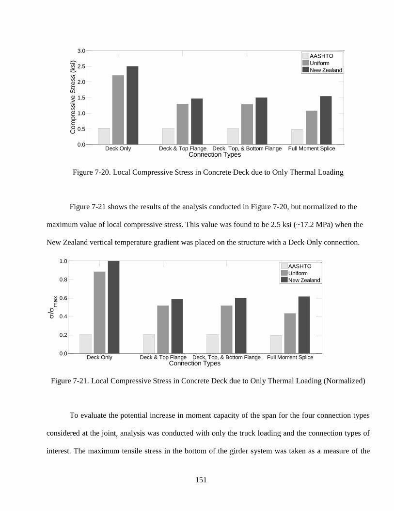
151
Figure 7-20. Local Compressive Stress in Concrete Deck due to Only Thermal Loading
Figure 7-21 shows the results of the analysis conducted in Figure 7-20, but normalized to the
maximum value of local compressive stress. This value was found to be 2.5 ksi (~17.2 MPa) when the
New Zealand vertical temperature gradient was placed on the structure with a Deck Only connection.
Figure 7-21. Local Compressive Stress in Concrete Deck due to Only Thermal Loading (Normalized)
To evaluate the potential increase in moment capacity of the span for the four connection types
considered at the joint, analysis was conducted with only the truck loading and the connection types of
interest. The maximum tensile stress in the bottom of the girder system was taken as a measure of the
Deck Only Deck & Top Flange Deck, Top, & Bottom Flange Full Moment Splice0.0
0.5
1.0
1.5
2.0
2.5
3.0
Connection Types
Com
pre
ssiv
e S
tress (
ksi)
AASHTO
Uniform
New Zealand
Deck Only Deck & Top Flange Deck, Top, & Bottom Flange Full Moment Splice0.0
0.2
0.4
0.6
0.8
1.0
Connection Types
/
ma
x
AASHTO
Uniform
New Zealand
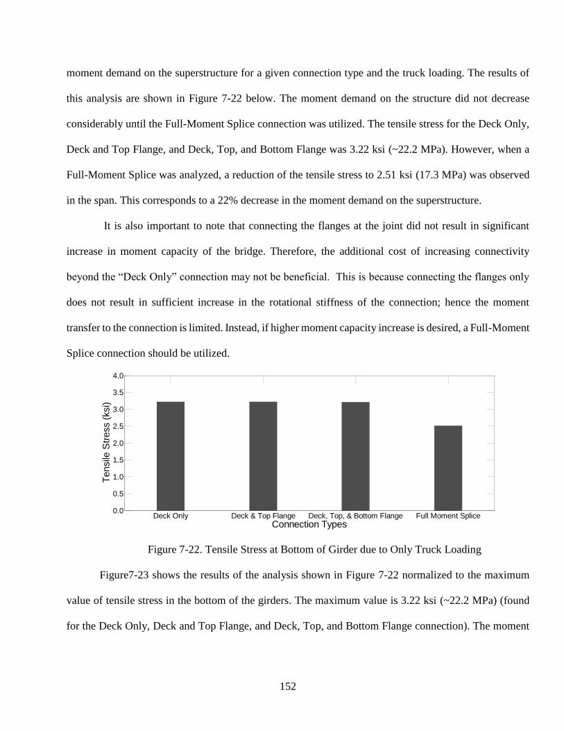
152
moment demand on the superstructure for a given connection type and the truck loading. The results of
this analysis are shown in Figure 7-22 below. The moment demand on the structure did not decrease
considerably until the Full-Moment Splice connection was utilized. The tensile stress for the Deck Only,
Deck and Top Flange, and Deck, Top, and Bottom Flange was 3.22 ksi (~22.2 MPa). However, when a
Full-Moment Splice was analyzed, a reduction of the tensile stress to 2.51 ksi (17.3 MPa) was observed
in the span. This corresponds to a 22% decrease in the moment demand on the superstructure.
It is also important to note that connecting the flanges at the joint did not result in significant
increase in moment capacity of the bridge. Therefore, the additional cost of increasing connectivity
beyond the “Deck Only” connection may not be beneficial. This is because connecting the flanges only
does not result in sufficient increase in the rotational stiffness of the connection; hence the moment
transfer to the connection is limited. Instead, if higher moment capacity increase is desired, a Full-Moment
Splice connection should be utilized.
Figure 7-22. Tensile Stress at Bottom of Girder due to Only Truck Loading
Figure7-23 shows the results of the analysis shown in Figure 7-22 normalized to the maximum
value of tensile stress in the bottom of the girders. The maximum value is 3.22 ksi (~22.2 MPa) (found
for the Deck Only, Deck and Top Flange, and Deck, Top, and Bottom Flange connection). The moment
Deck Only Deck & Top Flange Deck, Top, & Bottom Flange Full Moment Splice0.0
0.5
1.0
1.5
2.0
2.5
3.0
3.5
4.0
Connection Types
Tensile
Str
ess (
ksi)

153
demand on the superstructure for the Full-Moment Splice connection is approximately 78% of the
moment demand with the other connection types.
Figure 7-23. Tensile Stress at Bottom of Girder due to Only Truck Loading (Normalized)
After competition of analysis with separate thermal and truck loading, analysis was conducted
with both loads applied and the results are shown in Figure7-24 below. Due to the lesser amount of
compression resulting from the AASHTO thermal gradient (when only thermal loading is considered),
the stress at the bottom of the girders under combined AASHTO thermal gradient and truck loading
resulted in a tensile stress at the bottom of the girders. However, the Uniform and New Zealand vertical
thermal gradients induced enough compressive stress into the superstructure that the value of stresses in
the bottom of the girders remained compressive while the truckload was applied.
The maximum compressive stress demand in the girders near the bearings due to thermal and
truck loading was found when the Deck Only connection type was considered. The maximum
compressive stress demand in the girders when considering thermal gradients increased when the
connectivity of joint increased and the maximum values were found with a Full-Moment Splice
Connection. These results reiterate that the connection type at the joint influences the global performance
and moment demand on the bridge.
Deck Only Deck & Top Flange Deck, Top, & Bottom Flange Full Moment Splice0.0
0.2
0.4
0.6
0.8
1.0
Connection Types
/
ma
x

154
Figure 7-24. Stress at Bottom of Girder due to Thermal and Truck Loading
Figure 7-25 shows the results of the analysis shown in Figure 7-24 normalized to the maximum
value of tensile stress in the bottom of the girders for the AASHTO thermal gradient (3.84 ksi (~26.5
MPa)). The compressive values from the uniform and New Zealand thermal gradients are normalized to
the maximum value of compressive stress in the bottom of the girders (-6.15 ksi (~42.4 MPa)).
Figure 7-25. Stress at Bottom of Girder due to Thermal and Truck Loading (Normalized)
Deck Only Deck & Top Flange Deck, Top, & Bottom Flange Full Moment Splice-8
-6
-4
-2
0
2
4
6
8
Connection Types
Str
ess (
ksi)
AASHTO
Uniform
New Zealand
Deck Only Deck & Top Flange Deck, Top, & Bottom Flange Full Moment Splice-1.0
-0.5
0.0
0.5
1.0
Connection Types
/
ma
x
AASHTO
Uniform
New Zealand

155
7.9 Conclusion
The parametric study results highlighted differences between the thermal gradients considered.
The AASHTO described thermal gradient consistently resulted in lower stress demand on the structure
compared to the New Zealand thermal gradient. The results from the field data will aid in further
examination of the AASHTO described thermal gradient for bridges in Colorado.
The results also highlighted the extent of the effect that joint-removing connection types have
compared to clogged joints. The effect of the clogged joints was primarily localized at deck surface
behavior. However, the joint eliminating connection types influenced the global performance of the bridge
as well. No significant decrease in moment demand on the superstructure was observed until a full-
moment splice was utilized.

156
CHAPTER 8
LIFE-CYCLE COST ANALYSIS
8.1 Life-Cycle Cost Analysis Model
The goal of this chapter is to present and examine a LCCA that can be used to determine if it is
more cost effective to continue replacing bridge expansion joints as they deteriorate (i.e.no change to
current proactive) or to retrofit joints to be continuous. The approach is intended to be applicable to any
existing steel girder/concrete deck bridge; the characteristics of one typical northern Colorado steel plate
girder bridge with reinforced concrete abutments, deck, and pier caps are used as an example. The
example bridge is located in Northern Colorado and has three 75 ft (22.9 m) spans with five 44 in (1.1 m)
deep steel plate girders each, an 8 in (203mm) thick reinforced concrete composite deck, and finger
expansion joints.
An important step in conducting a LCCA is determining the appropriate costs to include in the
analysis. Two different LCCA Cost Scenarios are examined. Cost Scenario 1 considers costs directly
associated with expansion joints only, while Cost Scenario 2 considers costs associated with expansion
joints and damage to pier caps caused by leaking joints. It should be recognized that poorly maintained
expansion joints can lead to damage on other portions of a bridge. For example, road dirt and gravel can
clog joints, preventing them from closing when bridge temperatures increase. The clogging can lead to
damage at the joint as well as damage at abutments. Abutment damage can be a significant cost, and
would ideally be considered in LCCA, however, the amount of damage is very dependent on the abutment
design and the properties of the supporting soil. The potential for abutment damage is thus much more
bridge dependent and harder to generalize.

157
For each cost scenario, the first alternative is the current practice of replacing the joints after failure
without maintenance, also known as the do nothing or no change to current practice alternative. The
second alternative is retrofitting the joints after failure and accounting for cracking of the bridge deck due
to the negative moment induced at the continuous connection. Within each alternative differences in
results between two general locations, mountains and plains, will also be examined. Figure 8-1 shows the
flow chart of cost scenario to alternative to topographic location.
Figure 8-1 LCCA Cost Scenario
8.2 Life-Cycle Cost Analysis Equations and Variables
If all parts, consequences, and alternative actions on a structure, in this case bridge, can be
expressed monetarily then the best combination of actions or alternatives can be determined, as the one
that minimizes the total LCC of keeping the bridge in service. If each of the parts, consequences, and
alternatives are quantified there is also present a probability that that consequence or action will occur
causing that cost to become real.
Scenario X
Current Practice
Retrofit
Mountains
Plains
Plains
Mountains

158
There are two general LCC equations serving as the basis for this analysis, one for each alternative.
These general equations, shown below, include all possible parameter costs, where Eq. (8.1) is the LCC
for no change to current practice and Eq. (8.2) is the LCC for joint retrofitting.
LCCNC = Ci + Ccm + Co + CmPm + CrPr + CccPcc + CuPu - SV (8.1)
LCCJR= Ci + Ccm + CR+ Cs + Co + CmPm + CrPr + CccPcc + CuPu - SV (8.2)
Where Ci, Ccm, Co, CR, and Cs are the initial, construction, operation, retrofitting, and crack sealing
(if retrofit) costs. CmPm, CrPr, CccPcc, and CuPu are the maintenance, replacement, cost of capital and user
costs and their respective probabilities of occurrence. The maintenance term is composed of two parts,
CmPm = CcPc + CpcrPpcr, the joint maintenance (cleaning) and pier cap repair/maintenance and associated
probabilities. Finally, SV is the salvage value of the structure at the end of its life span.
While some of these costs and probabilities are obtainable or calculable based on information
from CDOT or testing, some are more ambiguous or not applicable to this particular LCCA. The initial
and construction costs are not applicable as this paper focuses on maintenance and repair decisions for
existing bridges only. The operation cost does not apply since this analysis is not focusing on drawbridges
or other bridges with daily operations. The user costs and costs of capital are more ambiguous; they are
an indirect cost, a cost of time and convenience to the using public and cost of initial investment, things
that are not easily quantifiable and as such are left out. Finally, because this paper focuses on the impact
of expansion joints on the LCC of a bridge the salvage value is not directly impacted and will show little
variation under different joint alternatives, for these reasons it is also left out of the analysis.
The adjusted equations are shown below as Eq (8.3) and (8.4). Additional terms will multiply
costs in order to account for the number of joints or linear feet of joint on the bridge.
LCCNC = CcPc + CpcrPpcr+ CrPr (8.3)
LCCJR= CcPc + CpcrPpcr + CrPr + CR + Cs (8.4)

159
Data collection and analysis were conducted to identify values for each of the variables indicated
in Eq (3) and (4). The costs associated with expansion joints and pier caps are shown in Table 8-1. The
costs were obtained from the CDOT business website from the 2014, 2015, and 2016 cost data books
(Colorado Dept. of Transportation 2016). These costs were taken as present value costs. According to
procedures described by the Federal Highway Administration, when performing a LCCA future costs are
determined by applying an inflation rate to present costs, while future costs are brought back to the present
by applying a discount rate. (FHWA, 2002). Inflation rates and especially discount rates can be difficult
to determine. This analysis used the present value costs directly, which assumes that the interest rate used
to bring these costs to future values throughout the LCC and the discount rate used to bring them from
future value back to present value offset each other.
Table 8-1 Assumed Costs Based on CDOT Data (Colorado Dept. of Transportation
2016)
Variable Value
Cost of Cleaning a Joint (Cc) $20/LF
Cost of Replacing a Joint (Cr) $350/LF
Cost of Removing/Retrofitting a Joint (CR) $205/LF
Cost of Sealing Cracks (Cs) $0.75/LF
Cost of Repairing Damaged Pier Caps (Cpcr) $2000/itema a These are estimates from CDOT, the costs are variable and site specific. Costs depend on amount of
damaged material and ease of access, both depend on extent of damage, traffic, and location of bridge. b Average life spans of bridge joints are based on CDOT personnel experience.
Other terms in the LCCA equation depended on agency practice or were bridge dependent. Values
for these variables are shown in Table 8-2. Case A represents CDOT general practices, according to
CDOT personnel in the Division of Project Support, and assumptions based on those practices. Because
Case A considers estimates and assumptions, Cases B and C consider two additional variations. Case B
considers increasing the time until joint replacement. Case C examines the effects of increasing the

160
remaining design life of the bridge, i.e. extending the period of analysis. Those values that are assumed
are listed first, as noted in the table, with the bridge dependent variables following. The agency practice
values are values that would vary depending on the exact DOT district practices. Bridge dependent
variables include the remaining design life of the bridge, the number of joints and abutment joints, and
the width of the bridge/length of the joint.
Table 8-2 Test Matrix Considering Agency and Bridge Dependent Variables
Variable Case A Common
CDOT
Practice
Case B Longer Joint
Replacement
Time
Case C
Longer
Remaining
Design Life
Prompt joint replacement a 0.5 yrs. 1 yrs. 0.5 yrs.
Max time to replace joint a 3.5 yrs. 4 yrs. 3.5 yrs.
Frequency a joint should be cleaneda 0.5 yrs. 0.5 yrs. 0.5 yrs.
Probability a joint will be cleaned
regularly a 0.0000001 0.0000001 0.0000001
Remaining design life (DL) 30 yrs. 30 yrs. 50 yrs.
Number of joints total 4 4 4
Number of abutment joints 2 2 2
Width of bridge 7.3 m (24ft) 7.3 m (24ft 7.3 m (24ft
a Assumed values based on CDOT general practices and discussions
For the LCC discussion and analysis, the LCCs from Case A are presented in tables for comparison
and discussion. The LCCs from Case A are used for analysis and discussion with the LCCs from Cases
B and C variables used for comparison when applicable.
8.3 Cost Scenario Equations, Variables, and Calculations
Each cost scenario adapts the two basic equations to its particular analysis of costs and variables.
The following describes the equations particular to each cost scenario and how the different variables are

161
calculated. Calculations for each cost scenario were conducted in MATLAB using the costs in Table 8-1
and agency practices in Table 8-2.
8.3.1 Cost Scenario 1
For Cost Scenario 1 equations (8.3) and (8.4) were modified to equations (8.5) and (8.6). The
probability for cleaning is assumed to be nearly zero as seen in Table 8-2 because CDOT and other DOTs
do not have the personnel or resources to clean/maintain expansion joints. This means the cost of joint
cleaning is effectively zero and was considered negligible in the calculations.
LCCNC = Cr (l j) (n) (8.5)
LCCJR = Cr (l j) (n)+ CR(N) + Cs(N) (DL) (8.6)
When calculating the costs for the no change alternative, the cost of a joint replacement, Cr, was
treated as a constant $350/linear ft and lj was taken as the total length of joints needing replacement. The
number of times joints were replaced on a bridge, n, was determined by simulating the bridge’s remaining
life. The joint life and time to failure were randomly simulated repetitively until the cumulative time spent
with intact and damaged joints reached the target for the remaining design life (DL). Uniform distributions
were assumed for the time to joint failure, and the time to joint replacement. Typical joint life spans were
provided by CDOT personnel in the Division of Project Support as two ranges, one for the plains and one
for the mountains. The joints located in the plains have a typical joint life span of seven to ten years and
joints located in the mountains have a typical joint life span of three to six years. Simulations of bridges
on the plains thus assumed joint life span was uniformly distributed between 7 and 10 years, for example.
The time to repair was simulated based on the typical repair times shown in Table 8-2. For example, for
Case A, the time to repair was assumed to be uniformly distributed between 0.5 and 3.5 years. All joints
on a bridge were assumed to fail and be repaired at the same time. This assumption was based on the
162
thought that it would be most efficient for repairs to take place on all joints at the same time, and joint
repairs on a bridge would not occur until all joints were in need of repair. The life cycle costs were
simulated a total of 10,000 times.
The cost calculation for the joint retrofit option was made for two different situations: retrofitting
only the deck joints – leaving the abutment joints in place - and retrofitting all joints on the bridge. When
only deck joints were retrofit, the length of joints needing repair, lj, included only the abutment joints,
when all joints were retrofit, lj was set equal to zero as the bridge had no remaining joints. When abutment
joints were left in, the cost for repair of abutment joints was calculated in the same way as the no change
case using random distributions to represent joint life and time to repair. CR is the cost to retrofit a joint
to make it continuous, and was taken as a fixed $205/linear ft. N is the number of joints that were retrofit
(either 2 or 4 depending on if the abutment joints were left in place or not). CS is the cost of crack sealing.
Crack sealing is only needed for those locations where a joint was removed and replaced with continuous
concrete. Crack sealing was assumed to occur once per year, and DL is the remaining design life assumed
for the analysis.
8.3.2 Cost Scenario 2
Cost Scenario 2 takes the equations from Cost Scenario 1 and adds the costs due to pier cap
corrosion due to leaking joints as shown in equations (8.7) and (8.8) below.
LCCNC = Cr (l j) (n) + Cpcr (m) (8.7)
LCCJR = Cr (l j) (n)+ CR(N) + Cs(N) (DL) + Cpcr (m) (8.8)
In addition to the variables determined for Cost Scenario 1 the number of times pier caps must be
repaired for corrosion damage during the remaining design life of the bridge, m, is needed. To estimate
this number, it was assumed that in the time between joint failure and joint repair the leaking joint allowed

163
chloride containing water to reach the pier caps below the bridge. Chlorides could then accumulate on the
surface of the pier and begin to diffuse through the concrete. When a sufficient concentration of chlorides
accumulated at the level of the reinforcement, corrosion could then begin, leading eventually to cracking
and spalling damage to the pier. The concentration of chlorides present on the pier cap is dependent on
the length of time the joint is leaking and the location of the bridge, i.e. how heavily de-icing salts are
used. The threshold concentration needed to start corrosion of the rebar is determined by the concrete mix,
clear cover, and type of rebar used (e.g. traditional bare bars, epoxy coated, stainless steel). In this analysis,
the threshold concentration and time to reach the threshold concentration were determined using the
software Life-365 developed under the American Concrete Institute (ACI) Committee 365 “Service Life
Prediction” and sponsored by ACI, the National Institute of Standards and Technology (NIST), and the
American Society for Testing and Materials (ASTM) in 1998.
Life-365 is a LCC and service life prediction tool for reinforced concrete structures exposed to
chlorides. The version used for this research is Version 2.2.2 released July 2013. The Life-365 software
does not account for carbonation as it has a low probability of occurrence and is often associated with
poor quality concrete (Life-365TM Consortium III. 2014). The software analysis is composed of four main
steps: predicting the corrosion initiation period, predicting the propagation period, estimating the
frequency and promptness of repair, and estimating the LCC. The repair and LCC portions of the software
are intended for concrete members and did not allow for including the costs related to bridge expansion
joints. Therefore, for the purpose of this research, results from the first two steps were utilized to
determine the time and concentration needed to corrode the rebar in bridge pier caps. The initiation period
is estimated using a simplified method based on Fickian diffusion. This method only requires a few inputs
from the user as discussed below. Furthermore, the model assumes that diffusion is the dominant
mechanism at play and that there are no cracks in the concrete in question. The diffusion coefficient used

164
is a function of time, temperature, and concrete mix composition. The equations for the diffusion
coefficient can be found in the Life-365 User’s Manual Section 2.1.1 (Life-365TM Consortium III. 2014).
Life-365 uses the type of structure, the geographical location, and the environmental exposure
input by the user to calculate the maximum chloride surface concentration corresponding to the threshold
chloride content at the level of the rebar and time to reach that concentration. The temperature profile
uses data compiled from meteorological data based on the geographical location input by the user. The
user can also manually input a temperature profile. The user can also define the concrete mix composition
and type of rebar present.
For the LCCA of leaking expansion joints in Colorado, Life-365 was utilized to determine the
time and chloride concentration at which corrosion is expected to begin and until the rebar becomes too
corroded to function. Urban bridges were selected as the structure type, the location chosen was Denver,
CO, the temperature profile for that location was used, and a basic concrete mixture without special
additives was assumed. Once these inputs were in place the model was run. The model produces a graph
of chloride surface concentration vs. time in years as seen in Figure 8-2 , this graph indicates that the
critical chloride concentration is reached after 9.2 years. As the remaining design life of the bridge was
simulated, the time to joint failure was randomly selected from the uniform distributions described
previously. Next the time until joint repair was randomly selected. During this time while the joint was
waiting for repair, it was assumed that chlorides could leak though the joint and accumulate on the pier
cap. When the total time of leaking reached 9.2 years, it was assumed that corrosion would initiate within
the pier cap. Life-365 then assumes that it would take 6 years (for uncoated reinforcing steel) for corrosion
damage to propagate through the pier cap to the point of requiring repair. As in Cost Scenario 1, the
remaining bridge service life was simulated 10,000 times.
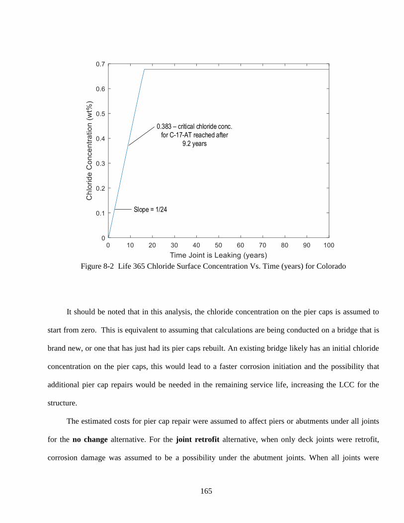
165
Figure 8-2 Life 365 Chloride Surface Concentration Vs. Time (years) for Colorado
It should be noted that in this analysis, the chloride concentration on the pier caps is assumed to
start from zero. This is equivalent to assuming that calculations are being conducted on a bridge that is
brand new, or one that has just had its pier caps rebuilt. An existing bridge likely has an initial chloride
concentration on the pier caps, this would lead to a faster corrosion initiation and the possibility that
additional pier cap repairs would be needed in the remaining service life, increasing the LCC for the
structure.
The estimated costs for pier cap repair were assumed to affect piers or abutments under all joints
for the no change alternative. For the joint retrofit alternative, when only deck joints were retrofit,
corrosion damage was assumed to be a possibility under the abutment joints. When all joints were
0.383 – critical chloride conc.
for C-17-AT reached after
9.2 years
Slope = 1/24

166
removed and replaced with continuous deck, costs for pier cap or abutment corrosion were assumed to
vanish as the continuous deck with crack sealing would prevent leaking of chloride solution onto the
elements below the deck.
8.4 Results
The MATLAB code was run for each combination of cost scenario and alternative agency practice
shown in Table 8-2. The results of these analyses were compiled to determine the most cost efficient
solution for existing bridge expansion joints.
8.4.1 Cost Scenario 1 Results
Cost Scenario 1 examines the LCCs for existing bridge joints only, without considering costs
associated with damage to the bridge’s superstructure. The costs associated with the two maintenance
alternatives and different topographical locations are shown in Table 8-3.
Table 8-3. LCC for Cost Scenario 1
Agency Practice Cases
A B C
Mean Std. Dev COV Mean Std. Dev COV Mean
Std.
Dev COV
Mo
un
tain
s
Leave Joints
In-place $138,805 $15,729 0.11 $128,328 $15,669 0.12 $242,199 $19,916 0.08
Retrofit deck
joints only $80,292 $7,801 0.10 $75,153 $7,754 0.10 $132,874 $9,876 0.07
Retrofit deck
and abutment
joints
$21,840 -- -- $21,840 -- -- $23,280 -- --
Pla
ins
Leave Joints
In-place $75,301 $14,373 0.19 $69,878 $9,100 0.13 $140,673 $13,102 0.09
Retrofit deck
joints only $48,782 $7,311 0.15 $45,834 $4,511 0.10 $81,795 $6,423 0.08
Retrofit deck
and abutment
joints
$21,840 -- -- $21,840 -- -- $23,280 -- --

167
For both the mountains and plains, and for all agency practice cases, there are significant cost
savings associated with retrofitting the bridges to remove expansion joints. Removing just the deck joints
can result in a 30-40% cost savings over the design life. Removing all bridge joints results in even greater
savings. The cost savings are highest in the mountains because the typical life of a joint in the mountains
is much shorter and thus when joints are allowed to remain in the bridges they will need to be replaced
much more often. The costs for agency practice case B are lower than those for case A because the time
until joints are replaced is longer, which means there will be fewer joint replacements over the remaining
life. The costs associated with leaving joints in place and continuing to repair/replace them when
necessary are much higher in agency practice case C, and the potential savings associated with removal
of joints are even larger.
This analysis shows that even on a single bridge there is the potential for significant savings by
removing either deck joints, or deck and abutment joints. When prioritizing bridges for the joint retrofit,
the greatest future savings can be achieved by retrofitting bridges in the mountains and those with longer
remaining design lives first. There is uncertainty associated with all of these cost estimates. Each
individual bridge and joint will behave in its own way, and the probabilistic distributions assumed in this
analysis are approximations based on prior CDOT experience. Given the assumed distributions, for most
of the alternatives and agency practice cases the coefficient of variation (COV) of LCC is in the range of
10%. There is higher variation for the Plains and agency practice Case A because the combination of
average joint life and average time to replacement is such that there is more variation in the number of
times the joints will be replaced within the remaining design life.
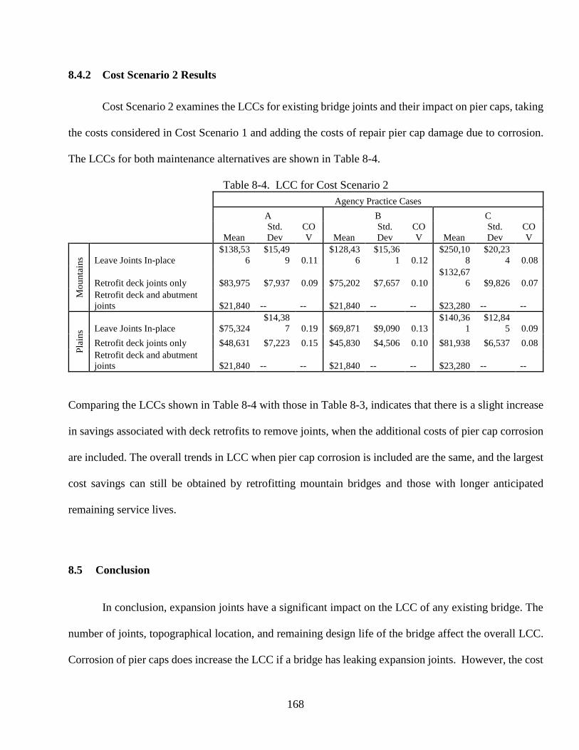
168
8.4.2 Cost Scenario 2 Results
Cost Scenario 2 examines the LCCs for existing bridge joints and their impact on pier caps, taking
the costs considered in Cost Scenario 1 and adding the costs of repair pier cap damage due to corrosion.
The LCCs for both maintenance alternatives are shown in Table 8-4.
Table 8-4. LCC for Cost Scenario 2
Agency Practice Cases
A B C
Mean
Std.
Dev
CO
V Mean
Std.
Dev
CO
V Mean
Std.
Dev
CO
V
Mo
un
tain
s Leave Joints In-place
$138,53
6
$15,49
9 0.11
$128,43
6
$15,36
1 0.12
$250,10
8
$20,23
4 0.08
Retrofit deck joints only $83,975 $7,937 0.09 $75,202 $7,657 0.10
$132,67
6 $9,826 0.07
Retrofit deck and abutment
joints $21,840 -- -- $21,840 -- -- $23,280 -- --
Pla
ins Leave Joints In-place $75,324
$14,38
7 0.19 $69,871 $9,090 0.13
$140,36
1
$12,84
5 0.09
Retrofit deck joints only $48,631 $7,223 0.15 $45,830 $4,506 0.10 $81,938 $6,537 0.08
Retrofit deck and abutment
joints $21,840 -- -- $21,840 -- -- $23,280 -- --
Comparing the LCCs shown in Table 8-4 with those in Table 8-3, indicates that there is a slight increase
in savings associated with deck retrofits to remove joints, when the additional costs of pier cap corrosion
are included. The overall trends in LCC when pier cap corrosion is included are the same, and the largest
cost savings can still be obtained by retrofitting mountain bridges and those with longer anticipated
remaining service lives.
8.5 Conclusion
In conclusion, expansion joints have a significant impact on the LCC of any existing bridge. The
number of joints, topographical location, and remaining design life of the bridge affect the overall LCC.
Corrosion of pier caps does increase the LCC if a bridge has leaking expansion joints. However, the cost

169
of joint replacement is still the dominant component in the total LCC, and for the purpose of making
decisions about which bridges should be retrofit a simplified LCCA considering only the joints
themselves should give appropriate information for decision making.
Retrofitting bridge deck joints while leaving the abutment joints in place creates a semi-integral
bridge design. This design still produces significant cost savings but allows the abutment joints to remain
and serve as thermal stress mediators. Additional study of the costs and consequences of abutment damage
due to clogged joints and or retrofit of abutment joints to be continuous is recommended before bridges
are retrofit to remove all joints.

170
CHAPTER 9
SUMMARY AND CONCLUSIONS
9.1 Summary
To gain further knowledge of thermal loading and its influence on expansion joint removal
practices, several tasks were performed in the completion of this thesis. First, an extensive literature
review was conducted to gain an understanding of the current research that has been completed in this
field of study. Moreover, a steel plate girder bridge and a reinforced concrete bridge in Colorado with
simply supported spans separated by expansion joints were selected for field instrumentation, load testing,
and long-term monitoring. In addition, a three-dimensional finite element model of this bridge was
developed using shell elements in CSi Bridge.
The selected bridges were instrumented with thermocouples, linear potentiometers, strain gauges,
and a scratch gauge. The sensors installed on the bridge provide thermal loading data throughout the depth
of the girders. The strain gauges provided information on bridge performance and local behavior at the
joint. The linear potentiometers provided information about how much the joint is moving throughout the
seasons and the day. The strain gauge installed at the center girder at midspan of the bridge were used to
validate the finite element model and an excellent match was achieved.
Following, field instrumentation, load testing, and validation of the numerical models, a
parametric study was performed to examine the effects of different connection types at the joint, different
thermal gradients, and the effect of clogged joints. For the steel bridge, the moment demand on the
structure was not significantly reduced until a Full Moment Splice connection was implemented. The
clogged joints did not affect the global behavior of the bridge significantly. The AASHTO described
thermal gradient resulted in smallest thermal stresses on the superstructure compared to the New Zealand

171
thermal gradient. Future analysis, using measured thermal gradient information collected from the bridge,
will be used to further calibrate the numerical model using a realistic thermal distribution.
In order to conduct a LCCA to compare joint maintenance options and expand knowledge of
thermal gradient effects on expansion joints in existing bridges, several tasks were conducted for the
completion of this thesis. First, an extensive literature review was conducted to further understanding of
current research into LCCA for expansion joints on existing bridges. From this literature review, general
LCC equations were generated for existing bridges with expansion joints and for retrofitting bridges to
remove joints. The LCCA was conducted using MATLAB as the main coding tool and data from CDOT,
LIFE 365, and the CSiBridge models. This analysis examined costs associated with bridge expansion
joints alone as well as those costs to the bridge superstructure, such as the bridge abutments and pier caps,
due to failing expansion joints. The analysis accounted for the bridge’s remaining design life, material
and location, where appropriate. The analysis was conducted for three different test scenarios, each
varying different parameters in order to provide a more comprehensive analysis. The analysis found that
retrofitting all joints except abutment joints to be continuous was the most cost effective in most cases,
assuming expansion joints will not be cleaned and maintained regularly.
9.2 Significance and Further Research
The significance of this work includes the results of the data collection and analysis, the parametric
study, and the LCCA findings. The daily temperature changes, thermal gradients, and overall shifts in
temperature due to changing seasons have a significant effect on bridge expansion joints in Colorado. The
potential for 0.01 in of movement and 0.5 ksi in stress increase on concrete bridges consistently and 0.5
in movement and 5 ksi stress on steel bridges regularly is not negligible. The preliminary data on the
concrete bridge C-17-AT presented in this report only accounts for mid-winter and does not account for
172
the hottest or coldest days of the year with the most movement. However, these limited observations do
imply that if CDOT is interested in removing an expansion joint, the bridge superstructure and retrofit
option would need to support the movement of the bridge. Additionally, there are clear differences
between the AASHTO gradient and what was observed in this study - and there is greater interest around
the country in bridges with fewer joints (either integral, semi-integral, and retrofitted). Undoubtedly,
instrumenting bridges for temperature effects is an important topic that might warrant a pooled fund study
to further evaluate the conclusions made in this study.
The parametric study and data analysis of thermal gradients indicate a stark need for further
research into thermal gradients experienced by bridges. The current standards of AASHTO and New
Zealand thermal gradients appear overly conservative and in need of refinement regarding shape
compared to the measured data. The extent of conservatism in the AASHTO gradient results, varying
from approximately 1.5 to 15 times that of the uniform gradient in this study, will depend in large on the
bridge configuration and type as well as the components for which the stresses are calculated.
Finally, the LCCA concluded that a semi-integral bridge design, which retrofits the interior
expansion joints of an existing bridge would provide the most cost effective design by decreasing joint
replacement costs and pier cap corrosion. Further research could expand on this LCCA by examining
environmental impacts and costs to users due to deteriorated expansion joints.

173
REFERENCES
AASHTO LRFD Bridge Design Specifications. (2012).
Agency, Highways, and River Severn. 2000. “Assessment of Composite Bridges,” 219–30.
Albhaisi, S., and Nassif, H. (2014). Simple Approach to Calculate Displacement and Rotations in
Integral Abutment Bridges.
Al-Wazeer, Adel, Bobby Harris, and Christopher Nutakor. 2005. “Applying LCCA to Bridges.” Public
Roads 69 (3): 9–9.
Basim, Mohammad Ch., and Homayoon E. Estekanchi. 2015. “Application of Endurance Time Method
in Performance-Based Optimum Design of Structures.” Structural Safety 56. Elsevier Ltd: 52–67.
doi:10.1016/j.strusafe.2015.05.005.
Board, Capital Development. 1998. “Life Cycle Cost Analysis Service.” World Pumps 1998 (376): 4.
doi:10.1016/S0262-1762(98)90545-4.
Briaud, L. (2013). Geotechnical Engineering: Unsaturated and Saturated Soils. Wiley, New
YorkCDOT. (2012). Bridge Design Manual.
Burke Jr., M. P. (1990). “The Integrated Constuction and Conversion of Single and Multiple Span
Bridges.” Bridge Management, 677–693.
“Congress Approves the Federal-Aid Highway Act.” (n.d.). United States Senate: Art & History,
<https://www.senate.gov/artandhistory/history/minute/Federal_Highway_Act.htm> (Mar. 7, 2014).
CDOT. 2015. “Bridge Expansion Device (0-4).” Colorado Dept. of Transportation. (2016).
“Engineering Estimates and Market Analysis.” <https://www.codot.gov/business/business/eema>
(Jan. 19, 2017).
Chen, Q. (2008). “Effects of Thermal Loads on Texas Steel Bridges.”
Federal Highway Administration. (n.d.). “History of the Interstate Highway System.”
<http://www.fhwa.dot.gov/interstate/history.htm> (July. 8, 2016).
French et al. (2013). “Investigation of Thermal Gradient Effects
in the I-35W St. Anthony Falls Bridge.” J. Bridge Engineering 18(1), 890-900
Frangopol, D M, and M Liu. 2007. “Structure and Infrastructure Engineering: Maintenance,
Management, Life-Cycle Design and Performance.” Structure and Infrastructure Engineering:
Maintenance, Management, Life-Cycle Design and Performance.
doi:10.1080/15732479.2013.769013.

174
Girmscheid, G. n.d. “Probabilistic Risk-Based LC NPV Model.” Zurich, Switzerland.
Goh, K. C., and Yang, J. 2014. “Managing Cost Implications for Highway Infrastructure
Sustainability.” International Journal of Environmental Science and Technology, 2271–80.
doi:10.1007/s13762-014-0572-5.
Hatami, A. and Morcous, G.. 2014. “Life-Cycle Cost Analysis for Bridge Managment An Application
to Nebraska Bridges.pdf.” ASCE.
Hawk, H.. 2003. Bridge Life-Cycle Cost Analysis. Edited by Transporation Research Board.
Washington D C: National Cooperative Highway Research Program.
Husain, I., and Bagnariol, D. (2000). “Design and Performance of Joinless Bridges in Ontario.”
Transportation Research Record, (1696), 109–121.
Kang, J, S Lee, T Hong, K.-J. Koo, C.-T. Hyun, and D Lee. 2007. “Life-Cycle Cost Analysis in Bridge
Structures: Focused on Superstructure.” 5th IABMAS Workshop on Life-Cycle Cost Analysis and
Design of Civil Infrastructure Systems, LCC05. London: Taylor & Francis Group.
http://www.scopus.com/inward/record.url?eid=2-s2.0-
84863266867&partnerID=40&md5=a7c7295395f718eee0e37cfdfb29a443.
Kassimali, A. (2012). Matrix Analysis of Structures, 2nd Ed., Cengage Learning, Independence, KY
Kim, S-H, Kim, J-H., Jung, C-Y., and Ahn, J-H. 2010. “Life-Cycle Cost Analysis of a TPSM Applied
Continuous Composite Girder Bridge.” International Journal of Steel Structures.
doi:10.1007/BF03215824.
“Life Cycle Cost Optimisation in Highway Concrete Bridges Management.pdf.” n.d. Life-365TM
Consortium III. (2014). “Life-365TM User Manual.” < http://www.life-
365.org/download/Life365_v2.2.1_Users_Manual.pdf> (Feb. 20, 2017).
Lam, C., Lai, D., Au, J., Lim, L., Young, W., and Tharmabala, B. (2008). “DEVELOPMENT OF
CONCRETE LINK SLABS TO ELIMINATE BRIDGE EXPANSION JOINTS OVER PIERS.”
Annual Conference of the Transportation Association of Canada, Toronto, Ontario, 1–20.
Li, D., Maes, M. A., and Dilger, W. H. (2008). “Evaluation of Temperature Data of Confederation
Bridge : Thermal Loading and Movement at Expansion Joint.”
Loveall, C. L. (1985). “Jointless Bridge Decks.” ASCE Journal of Civil Engineering, ASCE Journal of
Civil Engineering, 55(11), 64–67.
Mao, S., and Huang, R-Y. 2015. “Lifecycle Assessment of Maintennace Repair and Rehabilitation
Costs a Deterioration Modeling Approach for Bridge Components.” Journal of the Chinese
Institute of Civil and Hydraulic Engineering.
Lima, J. and de Brito, J.. 2010. “Managment Systems for Expansion Joints of Road Bridges.pdf.”

175
Milton, J. (2013). “Joint Maintenance and Best Practices in Deck Joint Replacement.” 2013 Virginia
Concrete Conference, Virginia Department of Transportation.
Moorty, S., and Roeder, C. W. (1992). “Temperature-Dependent Bridge Movements.” Journal of
Structural Engineering, 118(4), 1090–1105.
Ontario Ministry of Transportation. (2014). “Pulling the Teeth on Old Bridge Structures.” Road Talk,
<http://www.mto.gov.on.ca/english/transtek/roadtalk/rt17-1/#a8> (Apr. 9, 2014).
Osman, H. 2005. “Risk-Based Life-Cycle Cost Analysis of Privatized Infrastructure.” Transportation
Research Record. doi:10.3141/1924-24.
Ozbay, K., Jawad, D., Parker, N., Hussain, S.. 2004. “Life Cycle Cost Analysis: State-of-the-Practice vs
State-of-the-Art.” Washinton D.C.: National Academy of Science.
Precast/Prestressed Concrete Institute. (2003). Chapter 7: Loads & Load Distribution. In PCI
Bridge Design Manual. Chicago.
Pugasap, K., Kim, W., and Laman, J. A. (2009). “Long-Term Response Prediction of Integral Abutment
Bridges.” Journal of Bridge Engineering, 14(April), 129–139.
Roeder, C. W. (2003). “Proposed Design Method for Thermal Bridge Movements.” Journal of Bridge
Engineering, 8(1), 12–19.
Rogers, C. E., and Schiefer, P. (2012). “Region Bridge Support Unit Bridge Field Services.” (January).
Rogers, C. E., Schiefer, P., and Bouvy, A. (2012). Alleviating the Effects of Pavement Growth on
Strucutres.
Rager, K. 2016. "Joint Elimination retrofits and Thermal Loading Analysis In Plate Girder Bridge
Using Health Monitoring and Finite Element Simulations." Colorado State University.
Reigle, Jennifer A., and John P. Zaniewski. 2002. “Risk-Based Life-Cycle Cost Analysis for Project-
Level Pavement Management.”
Riedel, T, Tiemann, N. Wahl, M., Ambler, T. 1998. “LCCA-Life Cycle Cost Analysis.”
RStudio. "RStudio." < https://www.rstudio.com/> (Feb. 10, 2016)
Safi, M., Sundquist, H. and Karoumi, R. 2015. “Cost-Efficient Procurement of Bridge Infrastructures by
Incorporating Life-Cycle Cost Analysis with Bridge Management Systems,” 1–12.
doi:10.1061/(ASCE)BE.1943-5592.0000673.
Savioz, P. Spuler, T. 2014. “Minimally Invasive Maintenance Refurbishment Options for Bridge
Expansion Joints.” Leiden: The Netherlands: CRC PRess/Balkema.

176
Tsiatas, G., and Boardman, W. G. (2002). Expansion Joint Elimination For Steel Highway Bridges.
Kingston, RI, 1–129.
University, Standford. 2005. “GUIDELINES FOR October 2005,” no. October.
Vasseghi, A. (2013). “Effect of Pier Section Reinforcement on Inelastic Behavior of Steel I-Girder
Bridges.” Journal of Bridge Engineering, 18(January), 31–41.
Wasserman, E. P. (1987). “Jointless Bridge Decks.” American Institute of Steel Construction, Inc.,
24(3), 93–100.
Wasserman, E. P. (1999). “Tennessee State Route 50 Bridge Over Happy Hollow Creek.” American Pci
Journal 44(5):26-36.
Wasserman, E. P. (2014). “Tennessee State Route 385 over the Wolf River Wetlands - A Precast
Solution” PCI National Bridge Conference.
Zhu, Z., Davidson, M. T., Asce, A. M., Harik, I. E., Asce, M., Sun, L., and Sandefur, K. (2010). “Effect
of Superstructure Temperature Changes on Intermediate Pier Foundation Stresses in Integral
Abutment Bridges.” 1–11.

177
APPENDIX A.
INSTRUMENTATION PLAN FOR C-17-AT
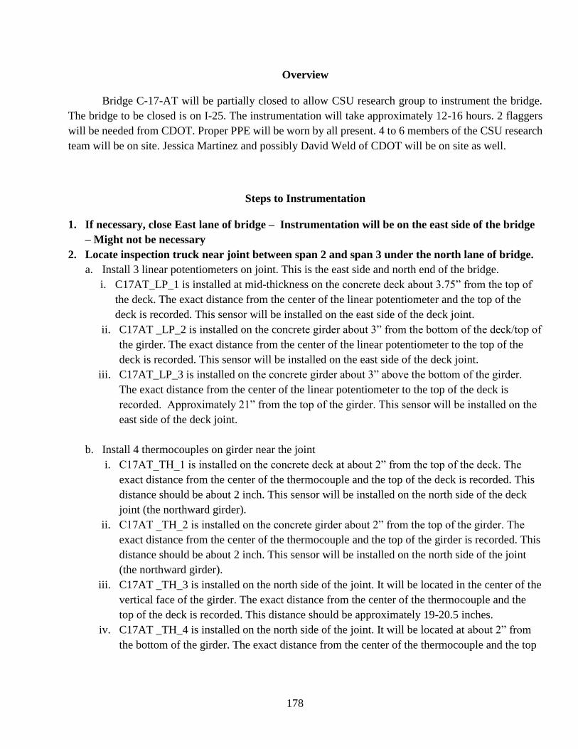
178
Overview
Bridge C-17-AT will be partially closed to allow CSU research group to instrument the bridge.
The bridge to be closed is on I-25. The instrumentation will take approximately 12-16 hours. 2 flaggers
will be needed from CDOT. Proper PPE will be worn by all present. 4 to 6 members of the CSU research
team will be on site. Jessica Martinez and possibly David Weld of CDOT will be on site as well.
Steps to Instrumentation
1. If necessary, close East lane of bridge – Instrumentation will be on the east side of the bridge
– Might not be necessary
2. Locate inspection truck near joint between span 2 and span 3 under the north lane of bridge.
a. Install 3 linear potentiometers on joint. This is the east side and north end of the bridge.
i. C17AT_LP_1 is installed at mid-thickness on the concrete deck about 3.75” from the top of
the deck. The exact distance from the center of the linear potentiometer and the top of the
deck is recorded. This sensor will be installed on the east side of the deck joint.
ii. C17AT _LP_2 is installed on the concrete girder about 3” from the bottom of the deck/top of
the girder. The exact distance from the center of the linear potentiometer to the top of the
deck is recorded. This sensor will be installed on the east side of the deck joint.
iii. C17AT_LP_3 is installed on the concrete girder about 3” above the bottom of the girder.
The exact distance from the center of the linear potentiometer to the top of the deck is
recorded. Approximately 21” from the top of the girder. This sensor will be installed on the
east side of the deck joint.
b. Install 4 thermocouples on girder near the joint
i. C17AT_TH_1 is installed on the concrete deck at about 2” from the top of the deck. The
exact distance from the center of the thermocouple and the top of the deck is recorded. This
distance should be about 2 inch. This sensor will be installed on the north side of the deck
joint (the northward girder).
ii. C17AT _TH_2 is installed on the concrete girder about 2” from the top of the girder. The
exact distance from the center of the thermocouple and the top of the girder is recorded. This
distance should be about 2 inch. This sensor will be installed on the north side of the joint
(the northward girder).
iii. C17AT _TH_3 is installed on the north side of the joint. It will be located in the center of the
vertical face of the girder. The exact distance from the center of the thermocouple and the
top of the deck is recorded. This distance should be approximately 19-20.5 inches.
iv. C17AT _TH_4 is installed on the north side of the joint. It will be located at about 2” from
the bottom of the girder. The exact distance from the center of the thermocouple and the top

179
of the deck is recorded. This distance should approximately 22 inches from the top of the
girder/2 inches from the bottom of the girder.
c. Install 8 strain gages on girder near the joint
i. C17AT _SG_1 is installed on the concrete deck as close to the top of the deck as possible.
The distance from the center of the strain gage and the top of the deck is recorded. This
distance should be about 1 inch. This sensor will be installed on the south side of the deck
joint (the southward girder).
ii. C17AT _SG_2 is installed on the concrete deck as close to the top of the deck as possible.
The distance from the center of the strain gage and the top of the deck is recorded. This
distance should be about 1 inch. This sensor will be installed on the north side of the deck
joint (the northward girder).
iii. C17AT _SG_3 is installed on the north side of the joint on the concrete deck as close to the
bottom of the deck as possible. The distance from the center of the strain gage and the top of
the deck is recorded. This distance should be about 6.5 inches from the top of the deck
(about 1in from the bottom of the deck). This sensor will be installed on the north side of the
deck joint (the northward girder).
iv. C17AT _SG_4 is installed on the north side of the joint. It will be located as close to the top
of the girder as possible. The distance from the center of the strain gage and the top of the
deck is recorded. This distance should be about 8.5 inches (about 1 in below the top of the
girder/bottom of the deck). This sensor will be installed on the north side of the deck joint
(the northward girder).
v. C17AT _SG_5 is installed on the north side of the joint. It will be located at mid depth of the
girder (about 12” from the bottom of the girder). The exact location from the bottom of the
girder will be measured and recorded. This sensor will be installed on the north side of the
deck joint (the northward girder).
vi. C17AT _SG_6 is installed on the south side of the joint. It will be located at the base of the
girder. The exact distance from the center of the strain gage and the top of the girder is
recorded. This distance should be about 23 inches/1 inch above the bottom of the girder. This
sensor will be installed on the south side of the deck joint (the southward girder).
vii. C17AT _SG_7 is installed on the north side of the joint. It will be located at the base of the
girder. The exact distance from the center of the strain gage and the top of the girder is
recorded. This distance should be about 23 inches/1 inch above the bottom of the girder.
This sensor will be installed on the north side of the deck joint (the northward girder).
3. Locate instrumentation Truck near mid-span of northernmost span under the East lane of the
bridge.
a. Install 1 strain gage on web of girder near bottom of web at mid-span. C17AT _SG_8 will be
installed as close to the bottom of the girder at mid-span as possible.

180
4. Zero strain gages and record linear potentiometer measurements for Control Load Testing??
5. Control Load Testing – To be done in the evening – Date & Time: TBA
a. Close easternmost (right) lane of bridge entirely – Drive truck over during gaps between
northbound traffic
b. During gaps in traffic drive CDOT specified truck to drive over bridge on closed lane 3x at 5
mph
c. During gaps in traffic drive CDOT specified truck to drive over bridge on closed lane 3x at 30
mph
d. During gaps in traffic drive have CDOT specified truck sit with front axil over midspan for 5
minutes
e. During gaps in traffic drive have CDOT specified truck sit with back axil over midspan for 5
minutes
f. Clean Up
g. Open bridge entirely
Detour Information
During the controlled load testing of the bridge, the east lane will need to be closed
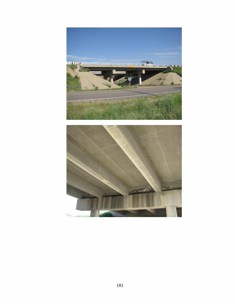
181

182
APPENDIX A
DECK JOINT REMOVAL SURVEY
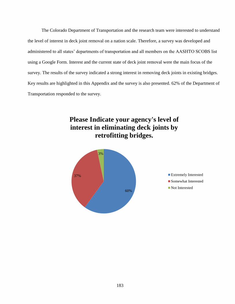
183
The Colorado Department of Transportation and the research team were interested to understand
the level of interest in deck joint removal on a nation scale. Therefore, a survey was developed and
administered to all states’ departments of transportation and all members on the AASHTO SCOBS list
using a Google Form. Interest and the current state of deck joint removal were the main focus of the
survey. The results of the survey indicated a strong interest in removing deck joints in existing bridges.
Key results are highlighted in this Appendix and the survey is also presented. 62% of the Department of
Transportation responded to the survey.
60%
37%
3%
Please Indicate your agency's level of
interest in eliminating deck joints by
retrofitting bridges.
Extremely Interested
Somewhat Interested
Not Interested
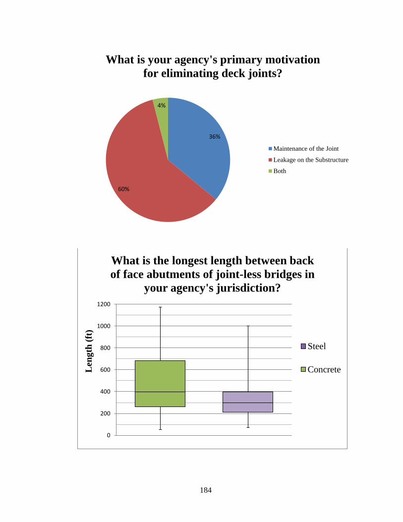
184
36%
60%
4%
What is your agency's primary motivation
for eliminating deck joints?
Maintenance of the Joint
Leakage on the Substructure
Both
0
200
400
600
800
1000
1200
Len
gth
(ft
)
What is the longest length between back
of face abutments of joint-less bridges in
your agency's jurisdiction?
Steel
Concrete

185
0%
10%
20%
30%
40%
50%
60%
Deck Only Deck and Top
Flange
Deck and
Bottom Flange
Deck, Top, and
Bottom Flange
Full-Moment
Splice
Concrete
Diaphragm
What connection types or details have been
used to eliminate deck joints in your
jurisdiction?

186
38%
8%
54%
Have improvements in maintenance costs or
other life cycle costs for retrofitted bridges
been observed as a result of deck joint
elimination?
Yes
No
Not sure

187
90%
10%
Does your agency promote newly
constructed bridges to be designed and built
without deck joints?
Yes
No

188

189

190

191

192

193

194
APPDEDIX C
INSTRUMENATION PLAN FOR B-16-FM
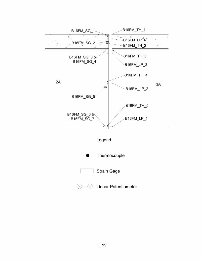
195
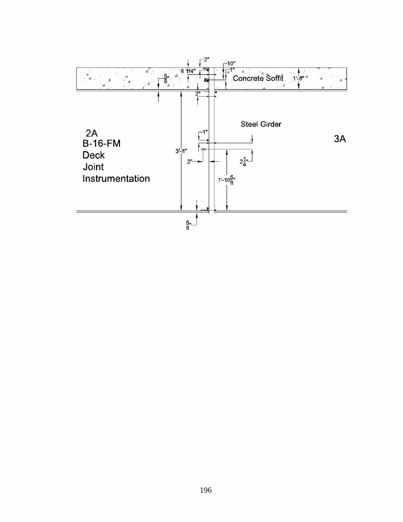
196