This is a repository copy of Joint Channel Estimation Algorithm via Weighted Homotopy forMassive MIMO OFDM System.

White Rose Research Online URL for this paper:http://eprints.whiterose.ac.uk/92693/

Version: Accepted Version

Article:

Nan, Y, Sun, X and Zhang, LX (2016) Joint Channel Estimation Algorithm via Weighted Homotopy for Massive MIMO OFDM System. Digital Signal Processing, 50. pp. 34-42. ISSN 1051-2004

https://doi.org/10.1016/j.dsp.2015.11.010

© 2015. This manuscript version is made available under the CC-BY-NC-ND 4.0 license http://creativecommons.org/licenses/by-nc-nd/4.0/

eprints@whiterose.ac.ukhttps://eprints.whiterose.ac.uk/

Reuse

Unless indicated otherwise, fulltext items are protected by copyright with all rights reserved. The copyright exception in section 29 of the Copyright, Designs and Patents Act 1988 allows the making of a single copy solely for the purpose of non-commercial research or private study within the limits of fair dealing. The publisher or other rights-holder may allow further reproduction and re-use of this version - refer to the White Rose Research Online record for this item. Where records identify the publisher as the copyright holder, users can verify any specific terms of use on the publisher’s website.

Takedown

If you consider content in White Rose Research Online to be in breach of UK law, please notify us by emailing eprints@whiterose.ac.uk including the URL of the record and the reason for the withdrawal request.

Joint Channel Estimation Algorithm via Weighted

Homotopy for Massive MIMO OFDM System

Yang Nana,1,∗, Xin Suna,1, Li Zhangb,1

aSchool of Electronics and Information Engineering, Beijing Jiaotong University, Beijing,

ChinabSchool of Electronic and Electrical Engineering, University of Leeds, Leeds, the United

Kingdom

Abstract

Massive (or large-scale) multiple-input multiple-output (MIMO) orthogonal fre-

quency division multiplexing (OFDM) system is widely acknowledged as a key

technology for future communication. One main challenge to implement this

system in practice is the high dimensional channel estimation, where the large

number of channel matrix entries requires prohibitively high computational com-

plexity. To solve this problem efficiently, a channel estimation approach using

few number of pilots is necessary. In this paper, we propose a weighted Ho-

motopy based channel estimation approach which utilizes the sparse nature in

MIMO channels to achieve a decent channel estimation performance with much

less pilot overhead. Moreover, inspired by the fact that MIMO channels are

observed to have approximately common support in a neighborhood, an in-

formation exchange strategy based on the proposed approach is developed to

further improve the estimation accuracy and reduce the required number of pi-

lots through joint channel estimation. Compared with the traditional sparse

channel estimation methods, the proposed approach can achieve more than 2dB

gain in terms of mean square error (MSE) with the same number of pilots, or

∗Corresponding authorEmail addresses: ynanbjtu@hotmail.com (Yang Nan), xsun@bjtu.edu.cn (Xin Sun),

l.x.zhang@Leeds.ac.uk (Li Zhang)1The authors would like to thank the supports by “the Fundamental Research Funds for

the Central Universities (2014YJS006)” and “National Natural Science Foundation of China(61201199)”.

Preprint submitted to Journal of LATEX Templates October 21, 2015

achieve the same performance with much less pilots.

Keywords: channel estimation, Massive MIMO OFDM, sparse recovery,

complex Homotopy

1. Introduction

The reliable high-speed broadband wireless links are expected to be on a huge

development prospective due to the foreseen rapidly increases in the number of

users, amount of data traffic and number of applications [1]. To meet these

demands, it is expected that future communication systems, i.e., beyond 4G5

or 5G systems, will reach a faster data rate at gigabit-scale over the next few

years. One of the recent proposed technologies for the future communication

system is the massive (or large-scale) multiple-input multiple-output (MIMO)

orthogonal frequency division multiplexing (OFDM) which is based on the same

concepts of the classical MIMO OFDM but with much larger number of antenna10

arrays on each side of the link. As such, the massive MIMO techniques could

provide unprecedented spectral efficiency and array gain that potentially meet

the rapidly growing demand for high data rates [2]. For instance, NTT DoCoMo

has performed the field experiment of a massive MIMO system with 12 × 12

antennas, which could reach the spectral efficiency of 50 bps/Hz and a data15

rate of 4.92 Gbps on the wireless channel with 100 MHz bandwidth [3], while

currently a 16× 16 MIMO configuration is considered by the evolution of WiFi

standard called IEEE 802.11 ac [4].

However, the very large number of channel matrix entries make the tradition-

al channel estimation strategy infeasible for frequency division duplex (FDD)20

protocol. Therefore, most researches on massive MIMO systems suggest the use

of time division duplex (TDD), where the channel state information (CSI) can

be acquired at the base station (BS) side and then utilized at both transmis-

sion directions based on the assumption of channel reciprocity [5]. However,

the inaccurate CSI acquired in the uplink can lead to significant performance25

degradation. Thus, accurate estimation of the high-dimensional MIMO channel

2

matrix in the uplink is critical for the deployment of massive MIMO.

Basically, there are two categories of channel estimation techniques for MI-

MO OFDM systems: blind estimation and pilots-based estimation. In [5],

a blind channel estimation technique based on the eigenvalue decomposition30

(EVD) has been proposed recently. Though this method could approach the n-

ear maximum-likelihood performance in theory, it has two shortcomings. Firstly,

it utilizes the sample covariance matrix as a substitution of the actual covariance

matrix to estimate the channel coefficients. Secondly, it assumes that the num-

ber of BS antennas is infinite. For these reasons, the EVD based method suffers35

from severe mean square error (MSE) performance penalty in practical dimen-

sional massive MIMO systems. Unlike the blind estimation techniques, several

pilot-based channel estimation schemes such as the Bayesian MMSE estimator

and minimum variance unbiased (MVU) have been adopted in MIMO system

[6][7]. However, the pilot overhead of those estimation schemes increases sharply40

in massive MIMO system where the number of antennas is very large. To solve

this problem, some recent works have exploited the sparse nature of the multi-

path channel and used compressive sensing (CS) based estimators to reconstruct

the channel perfectly with relatively less pilots [8][9]. Some CS algorithms, e.g.,

orthogonal matching pursuit (OMP) and basis pursuit (BP), have been already45

used in channel estimation for MIMO systems [9, 10, 11, 12]. However, neither of

these algorithms can attain accurate estimation performance and low complex-

ity at the same time. More recently, one quadratic semi-definite programming

(SDP) method has been discussed in [1], where the author demonstrated that

SDP solver can be stable and provide accurate channel estimation, as long as50

the degree of freedom (DoF) of the channel matrix is much smaller than the size

of channel matrix (i.e., total number of elements in the channel matrix). How-

ever, experimental results have shown that the convex optimization solver runs

slowly in the large-scale applications since it requires explicit operations on the

large matrix [13]. Therefore, scholars have abandoned the convex optimization55

based estimators and turned their attentions to the fast iterative methods.

The Homotopy algorithm has been originally proposed to solve noisy overde-

3

termined ℓ1-penalized least squares problems, which becomes popular quickly

since it can achieve the estimation accuracy as good as convex optimization

schemes with the estimation speed as fast as OMP [12]. Existing literature60

includes several improvements proposed for the standard Homotopy algorithm

[14, 15, 16, 17, 18]. One of the latest researches is the weighted Homotopy

in [15], which improves the original Homotopy by replacing its ℓ1 term with

a weighted ℓ1 term. However, this method can only work in the real domain,

which restricts its applications in the complex domain.65

In this paper, we propose a set of algorithms for channel estimation in mas-

sive MIMO systems. Firstly, we extend the conventional weighted Homotopy

to the complex field and adopt it to estimate the sparse channel on each BS

antenna. By adjusting the weight separately according to the channel coeffi-

cients, this approach improves the channel estimation performance with faster70

convergence rate. In addition, inspired by the fact that neighboring BS anten-

nas observe similar channel support (i.e., sparsity pattern) [19], we propose a

simple information sharing method between the BS antennas to further improve

the channel estimation performance. Compared with the conventional sparse

channel estimators, the required pilots in the proposed method is significantly75

reduced, leading to higher spectral efficiency, while its computational complexity

is proved to be much lower than the convex optimization solvers.

The rest of the paper proceeds as follows. We first describe the system model

and analyse the channel properties in Section 2. Then we propose the improved

Homotopy-based channel estimator in Section 3. A simple joint channel estima-80

tion method is presented in Section 4 while the performance analysis is provided

in Section 5. Numerical experiments are presented in Section 6. Finally, Section

7 concludes the paper.

Notations: Throughout this paper, matrices and vectors are denoted in bold

letters while the signals in frequency and time domains are represented by upper85

and lowercase characters, respectively. diag{x} is the diagonal matrix with

x on its main diagonal and min(·)+ means that the minimum is taken over

only positive arguments. Operators T and ∗ represent transpose and complex

4

conjugate transpose. | · |, ∥ · ∥p and sgn(·) denote absolute value, ℓp-norm and

sign function respectively. FN , C, R, IL, R, I represent the N ×N normalized90

discrete Fourier transform (DFT) matrix, the set of complex number, the set

of real number, the identity matrix with dimension L, the real part and the

imaginary part, respectively.

2. System model and problem formulation

2.1. System model95

Considering the uplink of a massive MIMO OFDM system where the BS

(receiver) is equipped with a large antenna array consisting of Nr = Mr ×Mc

antennas distributed across Mr rows and Mc columns∗ [19]. The BS simul-

taneously serves several UTs. Accordingly, for a certain UT the ith OFDM

symbol is composed of NCP -length cyclic prefix (CP) and N -length data block100

xi = [xi,0, . . . , xi,1, . . . , xi,N−1]T among which Np positions are randomly col-

lected to transmit the pilots [20]. Let p = [P1, · · · , Pj , · · · , PNp] (1 ≤ P1 < · · · <

Pj < · · · < PNp≤ N) where Pj denotes the index of the jth pilot. Thus the pi-

lots of the ith OFDM symbol can be expressed as x̄ i = [xi,P1, xi,P2

, · · · , xi,PNp].

For the kth receiving antenna at the BS side, the channel impulse response

(CIR) hki (1 ≤ k ≤ Nr) of the ith OFDM symbol can be represented as

hki = [hk

i,0, . . . , hki,l, . . . , h

ki,L−1]

T

where hki,l is the path gain of the lth path with the path delay τki,l, L is the maxi-

mum channel spread. Therefore, the received pilots yki = [yki,P1, yki,P2

, . . . , yki,PNp]

at the kth antenna can be denoted in the frequency domain as [20]

yki = diag{x̄ i}F p,Lh

ki + vk

i

= Pki h

ki + vk

i ,(1)

∗Note that although we focus on the rectangular array configuration in this paper, there

is no limitations for our approach to be applied to any other array configurations.

5

where diag{x̄ki } is a Np×Np diagonal matrix with x̄k

i on its diagonal, F p,L is a

partial discrete Fourier transform (DFT) matrix indexed by p = [P1, P2, · · · , PNp]

in row and [1, 2, · · · , L] in column from a standard N ×N DFT matrix, Pki =

diag{x̄ki }F p,L, v

ki denotes the additive white Gaussian noise (AWGN). For the

sake of brevity, without loss of generality we hereafter omit the script of i and

k unless these are required. Hence (1) becomes

y = Ph+ v . (2)

2.2. Channel properties105

Note that extensive literature has demonstrated that the wireless channels

are sparse in nature. This indicates that there are only few entries of the channel

matrix containing the significant fraction of the channel information while most

of the other entries are ignorable [21], [22] (e.g., the ITU Vehicular B channel

with 200 samples has only 6 resolvable paths [23]). As such we can draw a110

conclusion that the number of resolvable propagation paths (or most significant

taps) S is much smaller than the maximum channel spread L (S ≪ L).

Moreover, it is suggested in [24] that two channel taps are resolvable if the

time interval of arrival is larger than 110B where B is the bandwidth of signal.

Therefore, it is reasonable to assume that the CIRs measured at different BS

antennas share almost the same locations of the significant taps from a certain

transmitter if dmax

C≤ 1

10B , where dmax is the maximum distance between two

BS antennas and C is the speed of light. In other words, the path delays of

nonzero elements in CIRs between different transmit-receive pair are identical

while the path gains could be distinct, e.g.,

supp(hm) = supp(hn), m ̸= n, (3)

where hm is the CIR at the mth BS antenna, and supp(hm) denotes the support

of hm defined as

supp(hm) =

{ 1 hm(l) ̸= 0

0 hm(l) = 0, 0 ≤ l ≤ L− 1. (4)

6

In Table 1 we summarize the system parameters of two classical communica-

tion standards in terms of the bandwidth B, the maximum resolvable distance

Dmax and the distance between two adjacent antennas d = λ2 where λ is the115

signal wavelength [19]. It is clear that the antenna array could fall in one of the

two possible scenarios:

1) The antenna array has the common support when the maximum distance

between two antennas dmax ≤ Dmax. For example, consider a 16 × 16 array

in the 3GPP LTE standard, we have dmax = 15d < Dmax. Thus hk, k =120

1, 2, · · · , Nr have the common support. For convenience, we call such arrays

common support arrays (CSA).

2) The antenna array has the approximate support when dmax

C> 1

10B . For

the BS equipped with a large antenna array, e.g., 32 × 32 array where dmax =

31d > Dmax in the 3GPP LTE standard, the channel support varies across the125

array but with slow rate. We call such arrays the approximate support array

(ASA).

Table 1: Parameters of communication systems

Standard Bandwidth(B) Dmax = C10B d = λ

2

CDMA2000 1.25 MHz 24 m 0.15m

3GPP LTE 20 MHz 1.5 m 0.058m

While most of the recent literature in massive MIMO channel estimation

considers the common support case [25, 26], little attention has been paid to

the approximate support scenario. In this paper, we propose the approach that130

is applicable to both of the CSA and ASA cases with two steps:

1) Weighted Homotopy based channel estimation at each antenna, and

2) Joint channel estimation.

3. Weighted Homotopy based channel estimation

The set of channel estimation approaches that we propose in this paper use a135

modified version of the Homotopy algorithm proposed by the authors in [12] and

7

[15]. In this section, we first describe the standard Homotopy briefly, and then

propose our improved algorithm. Note that in this section the proposed channel

estimation algorithm is utilized at each BS antenna, where no cooperation occurs

among the antennas. The joint channel estimation strategy which considers both140

of the CSA and ASA cases will be issued in the next section.

3.1. Standard Homotopy

To estimate the CIR h in (2), we first introduce the famous convex opti-

mization model known as the Least Absolute Shrinkage and Selection Operator

(LASSO) or Basis Pursuit De-Noising (BPDN) as follows [27]:

minx

τ∥x∥1 +1

2∥Ax− y∥22 (5)

where y ∈ RNp×1 is the measurement vector, x ∈ R

L×1 is the unknown signal

of interest and A ∈ RNp×L is a known matrix. The ℓ1 term in (8) limits

the sparsity of the solution while the ℓ2 term keeps the solution close to the145

measurements. τ > 0 is a user-selected regularization parameter that transfers

ℓ1 minimization problem to ℓ2 minimization problem. The LASSO or BPDN

has been demonstrated to yield good performances in a variety of practical

applications [11][14][23]. One of the neoteric approaches for solving (5) is the

Homotopy algorithm, which traces a solution path for a range of decreasing150

values of τ , and terminates when τ converges to some threshold η [28]. The

solution path is followed by maintaining the optimality condition of (5) at each

point along the path.

Assume x̃ is the solution to (5). The Homotopy algorithm starts at x̃ =

0 and τ a large value which shrinks toward a threshold η in a sequence of

computationally inexpensive steps. At the same time, x̃ follows a piecewise-

linear path and converges to the solution of a noiseless sparse recovery problem,

denoted as

minx∥x∥1 s.t. y = Ax. (6)

In every Homotopy step, x̃ is updated according to two parameters: the step-

size and the update direction, both of which are determined by the support and

8

sign sequence of x̃. The support of x̃ changes only at certain critical values of

τ , when either a new nonzero element enters the support or an existing nonzero

element shrinks to zero. For every Homotopy step, we jump from one critical

value of τ to the next while updating the support of the solution, until τ is

reduced to its desired value. Specifically, let f(x) denote the objective function

of (5), the smaller critical value of τ can be easily obtained by calculating the

following equation [29]:

∂f(x) = A∗(Ax− y) + τ∂∥x∥1, (7)

where ∂∥x∥1 is the subgradient of ∥x∥1 obtained by

∂∥x∥1 =

{

z ∈ RL

∣

∣

∣

∣

zi = sgn(xi), xi ̸= 0

zi ∈ [−1, 1], xi = 0

}

,

where xi and zi account for the ith component of x and z, respectively. It is

clear that a necessary condition for x̃ to be the optimal value of (5) is that

A∗(Ax− y) + τ∂∥x∥1 = 0. (8)

Thus, let Γ = {i|x̃i ̸= 0} be the active support of x̃, x̃Γ be the vector with the

components of x̃ on support Γ and z = sgn(x̃Γ). At any given value of τ , we

have{

A∗Γ(Ax̃− y) = −τz (9a)

∥A∗Γc(Ax̃− y)∥∞ ≤ τ (9b)

where AΓ denotes a sub-matrix of A collecting the column vectors of A in

the active support Γ, and AΓc represents the sub-matrix collecting the column

vectors in the inactive support Γc where Γc = {i|x̃i = 0}. When we reduce τ by

a small value of δ, the new solution moves in a direction ∂x as

A∗Γ[A(x̃+ δ∂x)− y] = −(τ − δ)z

∥A∗Γc [A(x̃+ δ∂x)− y]∥∞ ≤ (τ − δ)

, (10)

and then we have

∂x =

(A∗ΓAΓ)

−1z on Γ

0 otherwise

. (11)

9

The solution will continue to move along the direction ∂x until one of the fol-

lowing two cases happens: (i) an element of x̃ shrinks to zero, which violates

(9a) and indicates this element should be removed from Γ, or (ii) an element in

Γc increases in magnitude beyond τ which violates (9b), and thus this element

should be added to Γ. Assume p = A∗Γc(Ax̃−y), d = A∗

ΓcA∂x , δ− and δ+ are

the step-sizes in cases (i) and (ii), respectively, then we can obtain the step-sizes

according to the following equations:{

x̃i + δ−∂xi = 0, i ∈ Γ (12a)

|pi + δ+di| = τ − δ+ (12b)

where pi and di are the ith element of p and d , x̃i and ∂xi are the ith element

of x̃ and the direction ∂x , respectively. Note that once an estimate x̃i decreases

to zero, it should be expelled from the active support, which explains why (12a)

is used as a constraint condition. Therefore, we have

δ− = mini∈Γ

(−x̃i

∂xi

)

+

. (13a)

Next, by solving (12b), we get the step-size δ+ as

δ+ = mini∈Γc

(

τ − pi1 + di

,−τ − pi−1 + di

)

+

, (13b)

The smallest step-size is obtained by selecting the smaller step-sizes as

δ = min(δ+, δ−). (14)

After that we get the new critical value of τ as τ = τ − δ and the new channel155

estimate x̃ as x̃ = x̃ + δ∂x. We repeat the above steps until τ decreases to a

desired threshold η.

3.2. Weighted Homotopy

To improve the recovery performance, it naturally leads us to substitute the

ℓ1 norm or ℓ2 norm in (5) for a weighted norm (see more details for the weighted

ℓ2 norm case in [16]-[18]). According to the system model discussed in Section

2, the weighted ℓ1 norm minimization problem could be described as

minh

L−1∑

i=0

wi|hi|+1

2∥Ph− y∥22 (15)

10

where y ∈ CNp×1 is the received signal vector, h ∈ C

L×1 is the unknown CIR

with hi the ith element, P ∈ CNp×L is the partial DFT matrix, and wi accounts160

for the weight of hi.

Note that all the quantities in (15) are complex-valued, except for wi a

positive real number. Thus, we first prove that the optimality conditions of the

complex weighted Homotopy could be still satisfied.

Lemma: h is the minimum of (15) if and only if there exists a complex

vector z which is the subgradient of |h|, satisfying zj =hj

|hj |if j ∈ {j|hj ̸= 0},

and |zj | ≤ 1 if j ∈ {j|hj = 0}, such that

wz +P∗(Ph−Y) = 0, (16)

where w = [w0, w1, · · · , wL−1].165

Proof: Denoting f(h) , w |h |+ 12∥Ph−Y∥22, which is the objective function of

(15) to be minimized. First we declare that, for j ∈ {j|hj ̸= 0}, (also expressed

as j ∈ act), we have

|hj + δhj | ≃ |hj |+R(h∗

jδhj)

|hj |,

where δhj is a small complex number. Also, for j ∈ {j|hj = 0} (j ∈ inact), we

have

|hj + δhj | = |δhj |.

Then by defining c , P∗(Ph−Y), successively we have

f(h+ δh)

≃ f(h) +1

2(δh∗c+ c∗δh) +

∑

j∈act

wjR(h∗jδhj)

|hj |+

∑

j∈inact

wj |δhj |

≃ f(h) +R(c∗δh) +∑

j∈act

wjR(h∗jδhj)

|hj |+

∑

j∈inact

wj |δhj |.

(17)

A necessary condition for h to minimize f(h) is ∂f(h) = 0, where ∂f(h) is the

derivative of f(h). Thus we have c + wz = 0. Then we can rewright the term

R(c∗δh) in (17) as the sum of two parts

R(c∗δh) = −R[(wz)∗δh]

= −∑

j∈act

wjR(h∗jδhj)

|hj |−

∑

j∈inact

wjR(z∗j δhj).(18)

11

Substituting (18) into (17), we have

f(h+ δh)

≃ f(h) +∑

j∈act

wj(−R(h∗

jδhj)

|hj |+

R(h∗jδhj)

|hj |)

+∑

j∈inact

wj(−R(z∗j δhj) + |δhj |)

≃ f(h) +∑

j∈inact

wj [1− |zj | cos(zj , δhj)]|δhj |.

It is obvious that 1 − |zj | cos(. . .) ≥ 0 if |zj | ≤ 1, then we can draw a

conclusion that f(h+ δh) ≥ f(h), and vice-versa.

From above discussion, we can see that the optimality conditions in (16)

are thus identical to (8) but with independent weight wi instead of τ , and the

subgradient ∂|h| obtained by

∂|h| ={

z ∈ CL

∣

∣

∣

∣

zj =hj

|hj |, hj ̸= 0

|zj | ≤ 1 , hj = 0

}

.

Thus we can urge the approximate CIR h̃ to converge towards the optimal

solution of (15) by decreasing the weights w separately as long as the optimality

condition is satisfied.170

Unlike the traditional Homotopy where τ controls the convergence speed of

all the estimates h on a same level, in the proposed method the independent

weight wi adjusts each estimate hi separately. To be specific, we let the weights

on the active support shrink at a faster rate, while the weights elsewhere shrink

at a slower rate. Thus, the estimates on the active support will be more likely175

to remain nonzero while the estimates on inactive support are driven to be zero,

whereby the proposed method could achieve more accurate estimation and faster

covergence rate.

In details, we take large values for all the weights wi as wi = maxj|P∗

j y|,i = 0, 1, . . . , L − 1 at the beginning, where Pj denotes the jth column in P.180

Then we divide these indices wi into the active set and the inactive set according

to the support of solution, e.g. we put wi into the active set if i ∈ Γ, otherwise

12

we put wi into the inactive set. Some desired values of wi are set at each

Homotopy step, to guarantee a faster reducing rate of wi in the active set and

a lower reducing rate of wi in the inactive set. Assume w̃i is the desired value185

of wi, we set w̃i in the active set as w̃i =wi

κ|h̃i|where h̃i is the solution of the

last iteration, and κ = Nr∥h̃∥2

2

∥h̃∥2

1

is a proportional constant [15]. It is advisable to

define κ in this manner because we can adjust the value of wi according to the

solution h̃ where the weight wi decreases to smaller value when Nr is large or

larger value when h̃ is denser. For the w̃i in the inactive set, we can select it in190

a variety of ways, e.g., we can set each of w̃i in the inactive set equal to maxj∈Γ

w̃j .

Next, by comparing (15) with (5), we can rewrite the constraint conditions

in (10) as follows:

{

P∗i (Ph̃− y) = −wizi, for all i ∈ Γ (19a)

|P∗i (Ph̃− y)| ≤ wi, for all i ∈ Γc (19b)

Define pi = Pi(Ph̃ − y) and di = PiP∂h. As we decrease wi toward the

desired weight w̃i, the solution h̃ moves in a direction ∂h as h̃ + δ∂h, which

must obey the constraint conditions

{

P∗Γ(Ph̃− y) + δ−P∗

ΓP∂h = −Wz+ δ−(W− W̃)z (20a)

|pi + δ+di| ≤ wi − δ+(wi − w̃i), i ∈ Γc (20b)

where z = h̃Γ

|h̃Γ|, h̃Γ is the vector with the components of h̃ on support Γ, W

and W̃ denote the |Γ| × |Γ| diagonal matrices whose elements of the primary

diagonal are the values of wi and w̃i on Γ, respectively.

Note that h̃i is a complex value. We can see from (12a) that the breakpoint

only occurs when both of the real part and imaginary part of h̃i (i ∈ Γ) shrink

to zero. In other words, if

R(h̃i)

R(∂hi)=

I(h̃i)

I(∂hi), i ∈ Γ (21)

we have

δ− = mini∈Γ

(−R(h̃i)

R(∂hi)

)

+

. (22a)

13

Thus, from (20b) we have

δ+ =

mini∈Γc

(

w2

i−|pi|2

2[R(p∗

idi)−siwi]

)

, |di| = 1

mini∈Γc

(

siwi−R(p∗

i di)−vi|di|2−s2

i

,siwi−R(p∗

i di)+vi

|di|2−s2i

)

, |di| ̸= 1

(22b)

where

si = w̃i − wi,

vi =√

[siwi −R(p∗i di)]2 − (s2i − |di|2)(w2

i − |pi|2).

Combining (19a) and (20a), we can get the update direction ∂h as:

∂h =

(P∗ΓPΓ)

−1(W− W̃)z on Γ

0 on Γc

. (23)

This process continues until all the weights w drop below a certain threshold η.195

Observing (21), we find that the condition in (21) is hard to be satisfied

since it only occurs when both of the real part and imaginary part of h̃i shrink

to zero simultaneously. That is to say, it is less likely to remove an element

from Γ than adding a new element into Γ. Meanwhile, the optimality condition

in (20b) indicates that as long as the inequality is satisfied, we can change the

corresponding weight in the inactive set to an arbitrary value while the solution

to (15) is still optimal. Therefore, we alter the selecting rule of δ in (14) as

follows. Suppose δ− makes an element h̃γ− (γ− ∈ Γ) decrease to zero. If

δ− < 1, then we remove γ− from Γ and set δ = δ−. Otherwise, we assume that

w has turned to w̃ and set δ = δ+ = 1. After that we select an index γ+ as

γ+ = argmaxi∈Γc |P∗i (Ph̃− y)|, (24)

and then add γ+ into Γ. In order to satisfy the inequality in (20b), we should

also change the choice strategy of the desired weight w̃i in the inactive set. By

substituting δ+ = 1 into (20b), we have w̃i ≥ |pi + di| for i ∈ Γc. Therefore,

we set the w̃i for i ∈ Γc either equal to |pi + di| or equal to maxj∈Γ

w̃j , whichever

is larger. For convenience, we name the proposed weighted Homotopy as WH200

14

Algorithm 1

1: Input: P, y and η

2: Output: h̃

3: Step 1. Initialization:

h̃← 0, wi ← maxj|P∗

j y| for all i, Γ← argmaxj |P∗j y|

4: Step 2.

While maxi

(wi) > η do

5: 1) Determine the desired weights value: w̃i =wi

κ|h̃i|for i ∈ Γ, and w̃i ←

max(|pi + di|,maxj∈Γ

w̃j) for i ∈ Γc

6: 2) Compute δ− in (22a)

7: 3) Compute ∂h in (23)

8: 4) Compute δ = min(1, δ−)

9: 5) h̃← h̃+ δ∂h

10: 6) wi ← wi + δ(w̃i − wi)

11: 7) if δ− < 1

Γ← Γ/γ− (removing γ− from Γ)

Else

γ+ = argmaxj∈Γc |P∗j (Ph̃− y)|

Γ← Γ ∪ γ+ (adding γ+ into Γ)

End if

End while

15

method and present the pseudocode in Algorithm 1.

Note that the WH method enhances the channel estimation performance

with faster convergence rate by adjusting the weights separately according to

the channel coefficients. To make further improvement, the common support of205

MIMO channels will be exploited and incorporated with WH method.

4. Joint channel estimation

In the joint channel estimation method, the BS antennas collaborate with

each other to take advantage of the common support (approximate support) of

the MIMO channels. Since this collaboration method is realized at the baseband,210

an additional processor on the baseband card is necessary [19].

The core idea of the collaboration strategy is that the antennas within a

“safety zone” share the information of the estimated channel support with each

other to improve the channel estimation performance. A safety zone is part of

the integrated antenna array where common support property is satisfied. In215

other words, the distance between any two antennas within the safety zone is no

larger than C10B . Therefore, it is safe to assume these antennas share the common

support of the CIRs. As a result, antennas in the same safety zone are able to

incorporate information from their neighbors to enhance its decision about the

support of the CIR, which will ultimately improve the channel estimation. Since220

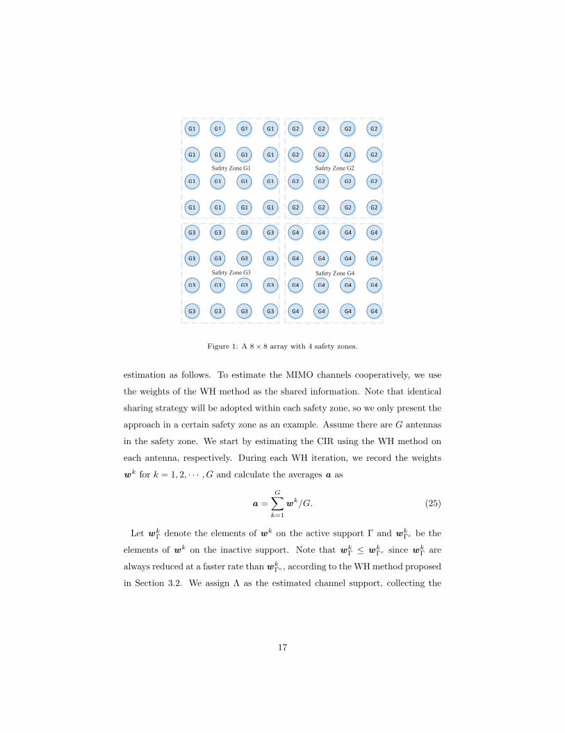
we consider the rectangular array configuration in this paper, the “safety zone”

is defined as a square containing G antennas. In Fig. 1 we use a 8×8 array with

4 safety zones as an example. Clearly, this strategy has two distinctive features:

1) It is flexible to change the size of safety zone according to the signal

bandwidth and antenna interval, which is critical to achieve the ASA.225

2) The communication overhead as well as the computational complexity are

reduced since there is no necessary to incorporate all the antennas for coopera-

tion.

Based on this information sharing strategy, we propose the joint channel

16

G1 G1

G1G1

G1 G1

G1G1

G1 G1

G1G1

G1 G1

G1G1

G2 G2

G2G2

G2 G2

G2G2

G2 G2

G2G2

G2 G2

G2G2

G3 G3

G3G3

G3 G3

G3G3

G3 G3

G3G3

G3 G3

G3G3

G4 G4

G4G4

G4 G4

G4G4

G4 G4

G4G4

G4 G4

G4G4

G1 G1

G1G1

G1 G1

G1G1

G1 G1

G1G1

G1 G1

G1G1

Safety Zone G1

G2 G2

G2G2

G2 G2

G2G2

G2 G2

G2G2

G2 G2

G2G2

Safety Zone G2

G3 G3

G3G3

G3 G3

G3G3

G3 G3

G3G3

G3 G3

G3G3

Safety Zone G3

G4 G4

G4G4

G4 G4

G4G4

G4 G4

G4G4

G4 G4

G4G4

Safety Zone G4

Figure 1: A 8× 8 array with 4 safety zones.

estimation as follows. To estimate the MIMO channels cooperatively, we use

the weights of the WH method as the shared information. Note that identical

sharing strategy will be adopted within each safety zone, so we only present the

approach in a certain safety zone as an example. Assume there are G antennas

in the safety zone. We start by estimating the CIR using the WH method on

each antenna, respectively. During each WH iteration, we record the weights

wk for k = 1, 2, · · · , G and calculate the averages a as

a =

G∑

k=1

wk/G. (25)

Let wkΓ denote the elements of wk on the active support Γ and wk

Γc be the

elements of wk on the inactive support. Note that wkΓ ≤ wk

Γc since wkΓ are

always reduced at a faster rate than wkΓc , according to the WH method proposed

in Section 3.2. We assign Λ as the estimated channel support, collecting the

17

indices of the S minimum values in a∗. After that we define a complementary

set ϖ = Γ − Λ that collects the indices which do not belong to the channel

support but are added to the active support accidentally. Then we define a

factor ν as

ν =maxi∈ϖ

(wki )

maxi∈Γc

(wki )

. (26)

Thus, we can refine the desired weights as

w̃ki =

{ w̃ki ν, for i ∈ Λ

w̃ki /ν, for i ∈ ϖ

. (27)

Note that we only adjust the desired weights in Γ and increase the w̃kϖ not

larger than the maxmimum of w̃kΓc due to the choice of ν. Therefore this230

modification will not violate the optimality conditions. Thus, in this fashion,

we can further reduce the weights on the set Λ and enlarge the weights on the

set ϖ while maintain the solution to be optimal. As a result, the elements

of h̃ on Λ will be encouraged to remain nonzero while the elements elsewhere

are driven to zero. This estimate will be more accurate since the antennas have235

shared their information to strengthen their beliefs about the estimated support

Λ. Note that this information sharing method can be regarded as an auxiliary

algorithm which should be included after Line 5 of Algorithm 1. The details of

this information sharing strategy is presented in Algorithm 2.

Algorithm 2

1) At every iteration, record the weights of WH method wk, k = 1, 2, · · · , G.

2) Compute the average weight a by (25).

3) Refine the the desired weights of each antenna according to (26) and (27).

It is worth noting that the proposed information sharing method is indepen-240

dent of the antenna array configuration. Since each antenna only utilizes the

∗The expected number of the active taps in the CIR can be detected by the iterative

support detection (ISD) method. For details, readers are referred to [30].

18

knowledge of their neighbors in the same safety zone, this method could im-

prove the channel estimation performance as long as the antennas are located

in the right safety zone, no matter what the topology of the antenna array. By

exploiting the common support of channel in WH method, the performance is245

clearly improved.

5. performance analysis

5.1. Boundary analysis

In the CSA case, since the channel support is assumed to be identical cross

the array, contribution from as many antennas as possible will always strengthen

the belief in the estimated support Λ. Hence, we may choose G = Nr which

indicates that all the BS antennas are included in one safety zone and share

channel information with each other. However, it might be unnecessary to

collect such a large number of antennas in one safety zone. In [19], the authors

have proposed a loose lower bound based on the lemma 1 in [31], where a

relationship between the number of antennas G, the sparsity of channel S and

the number of required pilots Np is established as

S ≤ ⌈(Np +G)/2− 1⌉, (28)

where ⌈·⌉ is the ceiling operation. Thus we can obtain the lower bound of G

accordingly as

G > 2S −Np. (29)

In the ASA case, the contribution of information sharing is based on how

fast the channel support change over the array. Clearly, if the support varies

fast, large number of G will lead to performance deterioration. Therefore, we

should select the number of antennas G that satisfies the CSA according to the

former discussion in Section 2.2. In other words, we could still get benefits from

information sharing by selecting a suitable G for the ASA case. Note that the

safety zone is considered as a square configuration in this paper. Therefore,

the distance between the farthest antennas in a safety zone with G antennas is

19

(√G−1)d. Therefore, to ensure the common support property in a safety zone,

G should satisfy the following inequation,

(√G− 1)d ≤ C

10B,

G ≤ ⌊( C

10Bd+ 1)2⌋,

(30)

where ⌊·⌋ is the floor operation.

5.2. Complexity analysis250

From [15] we know that the computational cost for one iteration of the s-

tandard Homotopy method is about GL + GQ + 3Q2 + O(L) FLOPs where

Q is the size of support Γ. By observing the proposed algorithm, we find the

proposed Homotopy algorithm requires roughly the same number of FLOPs as

the standard Homotopy algorithm plus additional computations to calculate the255

update direction ∂h in (23) where the weight matrix (W − W̃) is considered.

Since (W− W̃) is a Q×Q diagonal matrix, the additional cost for computing

∂h involves nearly Q2 FLOPs∗. As such, the computational complexity of one

iteration of the proposed Homotopy method is about GL + GQ + 4Q2 + O(L)

FLOPs, which is a little higher than that of the standard Homotopy method.260

However, due to the use of weights and information sharing method, the pro-

posed algorithm converges much faster than the standard Homotopy. Therefore,

the proposed algorithm requires fewer iterations, and thus less complexity (more

details will be shown in Section 6). Besides, in terms of the asymptotic com-

plexity, the standard Homotopy is roughly on the same order as OMP with265

O(G2L) while the asymptotic complexity of convex optimization algorithm is

about O(L3)[13]. Obviously, the complexity of the Homotopy method is less

than the convex optimization methods as long as the wireless channel is sparse.

∗For the sake of brevity, we neglect small complexity of scalar multiplications and additions

of matrices and vectors.

20

6. Simulation results

In this section, simulation studies are carried out to compare the performance270

of the proposed method with Homotopy† and two other CS algorithms: YALL1

[11] and OMP. YALL1 is a convex optimization algorithm which is proved to be

the best compared with two other famous BP algorithms including ℓ1-LS and

SpaRSA in [11], and OMP is widely used due to its fast convergence speed and

good estimation accuracy [5]. The threshold η for both of the standard Homo-275

topy and proposed Homotopy is 0.01 [15]. All the simulations in this paper are

performed using MATLAB 2012a, running on a standard computer with an Intel

Core i3-2100 CPU at 3.10GHz and 4GB of memory. A 16×16 MIMO configura-

tion is considered with the signal bandwidth of 20MHz at the central frequency

of 2.6GHz, as specified in the 3GPP-LTE standard. The number of OFDM280

subcarriers N is 4096, and the length of CP (NCP ) is 256 which could com-

bat channels with the maximum multi-path delay spread of 12.8µs. The sparse

Rayleigh channels with S = 6 significant taps and the maximum delay spread

of 10µs is considered. The IlmProp channel modeling tool [32] is employed for

the channel generations of both of the CSA and ASA scenarios. Specifically,285

we place point-like scatterers and the UT randomly and obstruct the line-of-

sight [19]. To make sure the desired sparsity S, we set the number of scatterers

accordingly and eliminate the small non-zero components in the resulting CIR

while maintain the top S components. Moreover, to generate the CSA and ASA

behavior, we set the antenna spacing d = 0.058m for CSA to satisfy the common290

support assumption while set the antenna spacing d = C20B = 0.75m for ASA to

ensure that the central antenna and its 8-neighbors have approximately common

support while the channel support of other antennas may change slowly.

Firstly, we set G = 9 and compare the success rate of the WH method with

other different channel estimators when a varying number of pilots Np is used295

†We have extended the standard Homotopy to the complex field in the similar way as the

proposed approach.

21

in Fig.2. The top row of Fig.2 shows the success rate of channel recovery when

the signal-to-noise ratio (SNR) SNR = 10dB while the bottom row shows the

success rate comparison when SNR = 20dB. The success rate is defined as the

ratio of the number of success trails to the number of total trails, where a trail is

recognized to be successful as the MSE is better than 10−2. It is obvious that all300

of the channel estimators require more pilots to achieve the MSE boundary of

10−2 when SNR decreases from 20dB to 10dB. However, when the same number

of pilots is used, WH method always obtains higher success rate in both of the

CSA and ASA scenarios. For example, In Fig.2(a) where SNR = 10dB, the

WH method uses only 60 pilots to achieve a success rate over 50% and 76 pilots305

to achieve 100% success rate. On the contrary, the traditional algorithms use at

least 68 pilots for the success rate over 50%, and none of them can achieve the

100% success rate due to the limitation of the SNR and the number of pilots.

Besides, for the ASA case as shown in Fig.2(b) and Fig.2(d), although the WH

performs not as well as it does in the CSA scenario, it still outperforms the310

traditional methods. Specifically, when Np = 60 is considered in Fig.2(b), the

WH achieves a success rate of 48% while the highest success rate the traditional

methods could attain is 27%.

Next, we investigate in Fig.3 the MSE performance comparison between the

proposed WH scheme and conventional OMP, YALL1 as well as the Homotopy315

scheme. In this experiment, we use G = 9 and Np = 32 pilots to estimate

the channel. It can be seen from the figure that for CSA the WH method

outperforms other three schemes by more than 2 dB when the target MSE of

10−2 is considered. To be specific, when the MSE is 10−2, OMP requires the

SNR of 24.8 dB, YALL1 and Homotopy require the SNR of 21.9 dB and 19.7320

dB, respectively, while the improved Homotopy needs only a SNR of 17.1 dB. It

is also worth noting that the WH method performs equally well for both CSA

and ASA, which demonstrates its robustness in the support-variant scenario.

Besides achieving the optimum MSE performance, another strength of the

WH method is its fast convergence. Next, we set G = 1 and compare the conver-325

gence speed of the WH method and Homotopy in Fig.4(a) (for SNR = 15dB)

22

40 50 60 70 800

0.2

0.4

0.6

0.8

1(a) CSA SNR=10dB

Number of pilots

Suc

cess

rat

e

40 50 60 70 800

0.2

0.4

0.6

0.8

1

Number of pilots

Suc

cess

rat

e

(b) ASA SNR=10dB

0 10 20 30 40 500

0.2

0.4

0.6

0.8

1(c) CSA SNR=20dB

Number of pilots

Suc

cess

rat

e

0 10 20 30 40 500

0.2

0.4

0.6

0.8

1

Number of pilots

Suc

cess

rat

e

(d) ASA SNR=20dB

OMP YALL1 Homotopy WH

Figure 2: Success rate comparison between different algorithms when a varying number of

pilots is used.

5 10 15 20 2510

−3

10−2

10−1

100

(a) CSA

SNR/dB

MS

E

5 10 15 20 2510

−3

10−2

10−1

100

(b) ASA

SNR/dB

MS

E

OMP YALL1 Homotopy WH method

Figure 3: MSE comparison between the WH method and conventional schemes.

23

5 10 15 20 250

5

10

15

20

25

30

35

40

45(a) SNR=15

Iterations

Ck

5 10 15 200

5

10

15

20

25

30

35

40

45(b) SNR=25

Iterations

Ck

Homotopy WH method

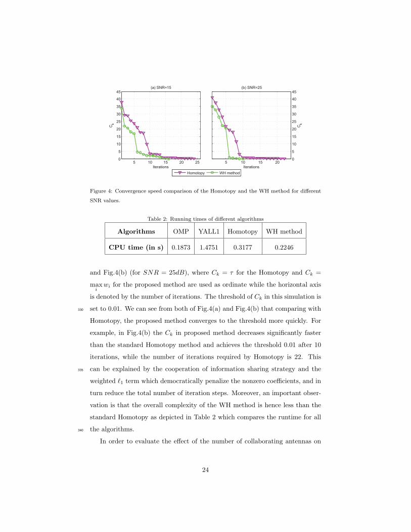
Figure 4: Convergence speed comparison of the Homotopy and the WH method for different

SNR values.

Table 2: Running times of different algorithms

Algorithms OMP YALL1 Homotopy WH method

CPU time (in s) 0.1873 1.4751 0.3177 0.2246

and Fig.4(b) (for SNR = 25dB), where Ck = τ for the Homotopy and Ck =

maxi

wi for the proposed method are used as ordinate while the horizontal axis

is denoted by the number of iterations. The threshold of Ck in this simulation is

set to 0.01. We can see from both of Fig.4(a) and Fig.4(b) that comparing with330

Homotopy, the proposed method converges to the threshold more quickly. For

example, in Fig.4(b) the Ck in proposed method decreases significantly faster

than the standard Homotopy method and achieves the threshold 0.01 after 10

iterations, while the number of iterations required by Homotopy is 22. This

can be explained by the cooperation of information sharing strategy and the335

weighted ℓ1 term which democratically penalize the nonzero coefficients, and in

turn reduce the total number of iteration steps. Moreover, an important obser-

vation is that the overall complexity of the WH method is hence less than the

standard Homotopy as depicted in Table 2 which compares the runtime for all

the algorithms.340

In order to evaluate the effect of the number of collaborating antennas on

24

5 10 15 20 2510

−3

10−2

10−1

100

(a) CSA

SNR/dB

MS

E

5 10 15 20 2510

−3

10−2

10−1

100

(b) ASA

SNR/dB

MS

E

G=1 G=4 G=9 G=16

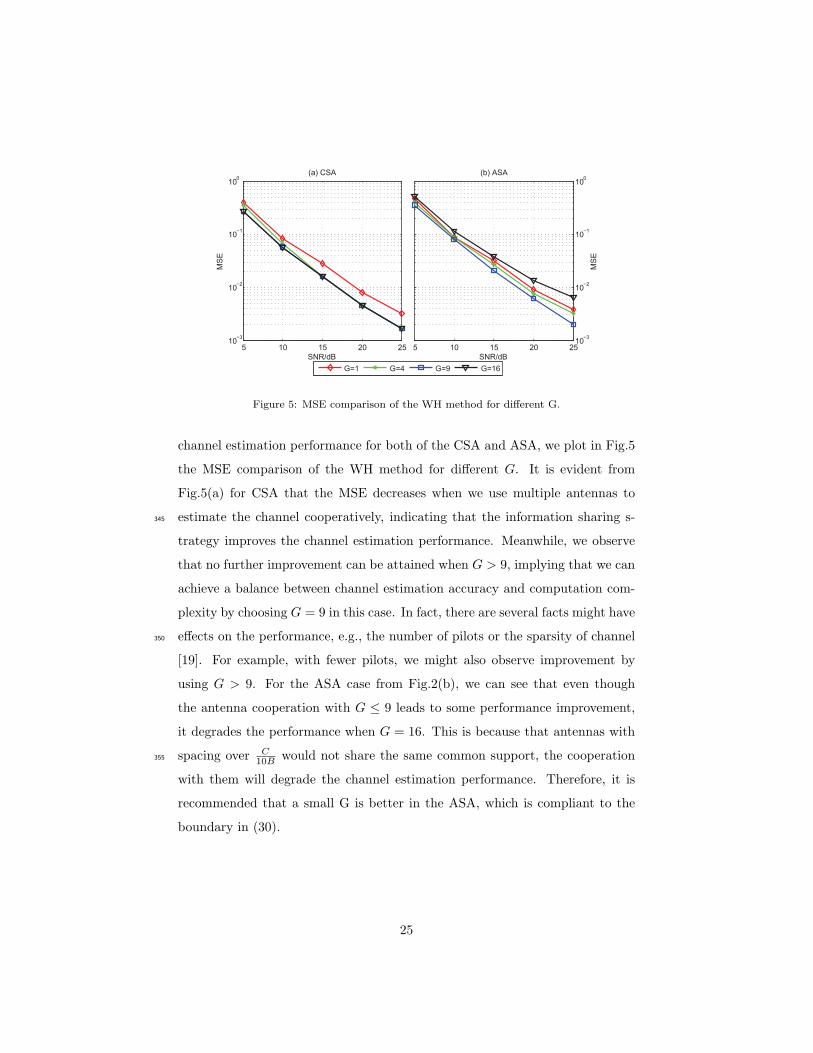
Figure 5: MSE comparison of the WH method for different G.

channel estimation performance for both of the CSA and ASA, we plot in Fig.5

the MSE comparison of the WH method for different G. It is evident from

Fig.5(a) for CSA that the MSE decreases when we use multiple antennas to

estimate the channel cooperatively, indicating that the information sharing s-345

trategy improves the channel estimation performance. Meanwhile, we observe

that no further improvement can be attained when G > 9, implying that we can

achieve a balance between channel estimation accuracy and computation com-

plexity by choosing G = 9 in this case. In fact, there are several facts might have

effects on the performance, e.g., the number of pilots or the sparsity of channel350

[19]. For example, with fewer pilots, we might also observe improvement by

using G > 9. For the ASA case from Fig.2(b), we can see that even though

the antenna cooperation with G ≤ 9 leads to some performance improvement,

it degrades the performance when G = 16. This is because that antennas with

spacing over C10B would not share the same common support, the cooperation355

with them will degrade the channel estimation performance. Therefore, it is

recommended that a small G is better in the ASA, which is compliant to the

boundary in (30).

25

7. Conclusion

In this paper, we proposed an improved Homotopy method, which adaptive-360

ly reweights the ℓ1 norm inside a Homotopy iteration, to estimate the massive

MIMO OFDM channel matrix. Since the proposed algorithm emphasizes more

on adding elements into the active set and less on removing elements from the

active set, it is appropriate to consider the approach as a compromise between

standard Homotopy and LARS which is similar with standard Homotopy but365

omits the step that removes variables from the active set [28]. In addition, to

further reduce the required pilots while enhance the estimation accuracy, we pro-

posed a Homotopy-based joint channel estimation method where the antennas

collaborate with their neighbors within the same safety zone. In the simulation-

s, we investigated how the estimation performance is affected by the number of370

pilots and cooperative antennas, and proved that the proposed approach can

yield high quality channel reconstructions in various scenarios while using small

number of pilots.

References

[1] S.Nguyen, A.Ghrayeb, Compressive sensing-based channel estimation for375

massive multiuser mimo systems, IEEE Wireless Communications and Net-

working Conference (WCNC) (2013) 2890–2895.

[2] N.Shariati, E.Bjornson, M.Bengtsson, M.Debbah, Low-complexity polyno-

mial channel estimation in large-scale mimo with arbitrary statistics, IEEE

Journal of Selected Topics in Signal Processing 8 (5) (2014) 815–830.380

[3] H.Taoka, K.Higuchi, Experiments on peak spectral efficiency of 50 bps/hz

with 12-by-12 mimo multiplexing for future broadband packet radio access,

International Symposium on Communications, Control and Signal Process-

ing (ISCCSP) (2010) 1–6.

[4] G.Breit, et al., Channel modeling, Doc. IEEE 802.11-09/0088r0.385

26

[5] H.Ngo, E.Larsson, Evd-based channel estimation in multicell multiuser mi-

mo systems with very large antenna arrays, IEEE International Conference

on Acoustics, Speech and Signal Processing (ICASSP) (2012) 3249–3252.

[6] S.Kay, Fundamentals of statistical signal processing: Estimation theory,

Fundamentals of Statistical Signal Processing.390

[7] J.Kotecha, A.Sayeed, Transmit signal design for optimal estimation of cor-

related mimo channels, IEEE Transactions on Signal Processing 52 (2)

(2004) 546–557.

[8] D.Donoho, I.Johnstone, A.Maleki, A.Montanari, Compressed sensing over

ℓp-balls: Minimax mean square error, IEEE International Symposium on395

Information Theory Proceedings (ISIT) (2011) 129–133.

[9] C.Berger, Z.Wang, J.Huang, S.Zhou, Application of compressive sensing to

sparse channel estimation, IEEE Communications Magazine 48 (11) (2010)

164–174.

[10] S.Nguyen, A.Ghrayeb, M.Hasna, Iterative compressive estimation and de-400

coding for network-channel-coded two-way relay sparse isi channels, IEEE

Communications Letters 16 (12) (2012) 1992–1995.

[11] J.Huang, C.Berger, S.Zhou, J.Huang, Comparison of basis pursuit algo-

rithms for sparse channel estimation in underwater acoustic ofdm, IEEE

OCEANS 2010 (2010) 1–6.405

[12] C.Qi, L.Wu, X.Wang, Underwater acoustic channel estimation via com-

plex homotopy, IEEE International Conference on Communications (ICC)

(2012) 3821–3825.

[13] D.Donoho, A.Maleki, A.Montanari, Message passing algorithms for com-

pressed sensing: I. motivation and construction, IEEE Information Theory410

Workshop (ITW) (2010) 1–5.

27

[14] W.Chen, M.Rodrigues, I.Wassell, Penalized ℓ1 minimization for reconstruc-

tion of time-varying sparse signals, IEEE International Conference on A-

coustics, Speech and Signal Processing (ICASSP) (2011) 3988–3991.

[15] M.Asif, J.Romberg, Fast and accurate algorithms for re-weighted ℓ1-norm415

minimization, IEEE Transactions on Signal Processing 61 (23) (2013) 5905–

5916.

[16] P.Holland, R.Welsch, Robust regression using iteratively reweighted least-

squares, Communications in Statistics Theory and Methods 6 (9) (1977)

813–827.420

[17] I.Gorodnitsky, B.Rao, Sparse signal reconstruction from limited data using

focuss: a re-weighted minimum norm algorithm, IEEE Transactions on

Signal Processing 45 (3) (1997) 600–616.

[18] I.Daubechies, R.DeVore, M.Fornasier, C.Gunturk, Iteratively reweighted

least squares minimization for sparse recovery, Communications on Pure425

and Applied Mathematics 63 (1) (2010) 1–38.

[19] M.Masood, L.Afify, T.AlNaffouri, Efficient coordinated recovery of sparse

channels in massive mimo, IEEE Transactions on Signal Processing 63 (1)

(2015) 104–118.

[20] L.Dai, Z.Wang, Z.Yang, Spectrally efficient time-frequency training ofdm430

for mobile large-scale mimo systems, IEEE Journal on Selected Areas in

Communications 31 (2) (2013) 251–263.

[21] E.Bonek, Experimental validation of analytical mimo channel models, e&i

Elektrotechnik und Informationstechnik 122 (6) (2005) 196–205.

[22] H.Ozcelik, N.Czink, E.Bonek, What makes a good mimo channel model?,435

IEEE Vehicular Technology Conference (2005) 156–160.

[23] Guideline for evaluation of radio transmission technology for imt-2000,

Tech. rep., Recommendation ITU-R M.1225.

28

[24] Y.Barbotin, A.Hormati, S.Rangan, M.Vetterli, Estimation of sparse mimo

channels with common support, IEEE Transactions on Communications440

60 (12) (2012) 3705–3716.

[25] Z.Gao, L.Dai, Z.Wang, Structured compressive sensing based superim-

posed pilot design in downlink large-scale mimo systems, Electronics Let-

ters 50 (12) (2014) 896–898.

[26] C.Qi, L.Wu, Uplink channel estimation for massive mimo systems exploring445

joint channel sparsity, Electronics Letters 50 (23) (2014) 1770–1772.

[27] A.Maleki, L.Anitori, Z.Yang, R.Baraniuk, Asymptotic analysis of complex

lasso via complex approximate message passing (camp), IEEE Transactions

on Information Theory 59 (7) (2013) 4290–4308.

[28] D.Donoho, Y.Tsaig, Fast solution of ℓ1-norm minimization problems when450

the solution may be sparse, IEEE Transactions on Information Theory

54 (11) (2008) 4789–4812.

[29] J.Fuchs, On sparse representations in arbitrary redundant bases, IEEE

Transactions on Information Theory 50 (6) (2004) 1341–1344.

[30] Y.Wang, W.Yin, Sparse signal reconstruction via iterative support detec-455

tion, SIAM J. Imaging Sci. 49 (6) (2010) 2543–2563.

[31] B.Rao, K.Engan, S.Cotter, Diversity measure minimization based method

for computing sparse solutions to linear inverse problems with multiple

measurement vectors, IEEE International Conference on Acoustics, Speech,

and Signal Processing (ICASSP ’04) (2004) 17–21.460

[32] Ilmprop, [Online]. Availabel: http://www.tu-ilmenau.de/nt/en/ilmprop

[Online; accessed Jan. 10, 2014].

29