First steps in digital signal processing

John Coleman

Phonetics LaboratoryUniversity of OxfordUniversity of Oxford

Analogue-to-digital conversion 1:

Sampling

Analogue-to-digital conversion 2:

Quantization

D-to-A, quantization error

D-to-A, quantization error

• To reduce the quantization error, use more levels • To reduce the quantization error, use more levels (dynamic range):

• 8 bits: 28 = 256 levels• 12 bits: 212 = 4096 levels• 16 bits: 216 = 65536 levels• 16 bits: 216 = 65536 levels

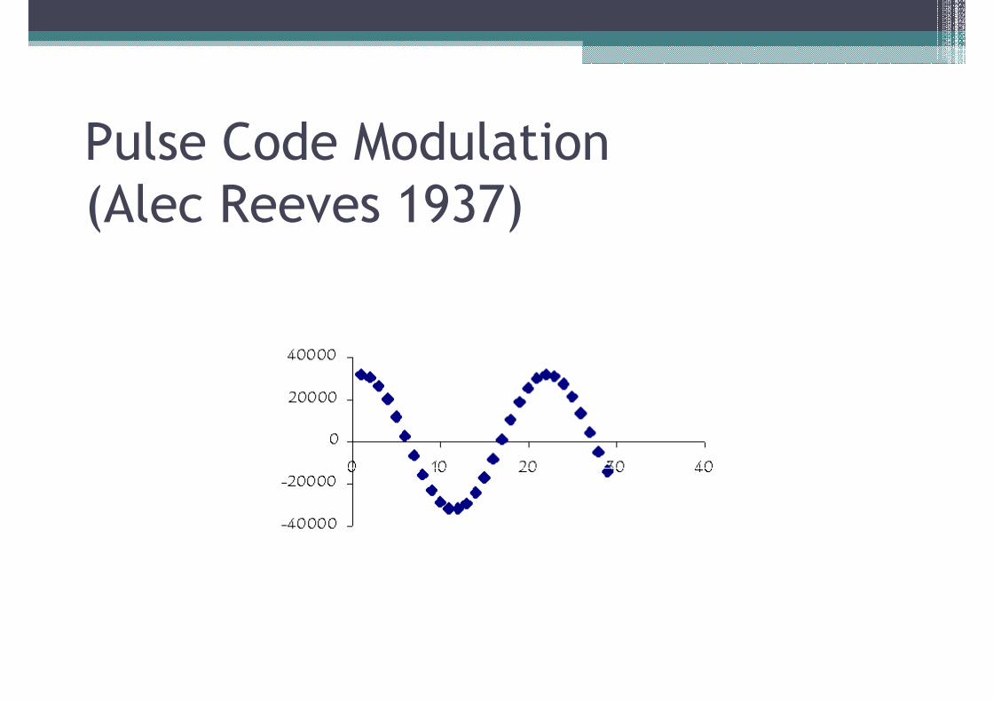
Pulse Code Modulation

(Alec Reeves 1937)

Sampling theorem; Nyquist frequency

• Sampling rate must be at least twice the highest frequency you want to capturefrequency you want to capture

Operations on sequences of numbers

• Let's call the sample number i and the i'th sample x[i]• Sum or integral, Σx[i]. • Sum or integral, Σx[i]. • If x[i] has positive and negative values, take |x[i]| the

absolute (i.e. unsigned) value of x[i]. • Or, first calculate the square of x[i], x[i]2, and then take

the square root, √(x[i]2). Σ√(x[i]2) is a measure of the overall energy of a signal.overall energy of a signal.

• x[i]2 gets bigger and bigger as x[i] gets longer. • The average amplitude of a signal, calculated over n

samples: √(Σx[i]2/n). This is called the root mean squareor RMS amplitude.

Local (moving) averagee.g., y[n] = ¼ x[n ] + ¼ x[n-1] + ¼ x[n-2] + ¼ x[n-3]

Local (moving) averageEffect: low-pass filtering

Time-domain filtering

4 samples is very short, so its effects are very local –high frequency components. To smooth over a high frequency components. To smooth over a larger slice of the signal, we can do two things:

a) increase the number of samples in x[n] ... x [n-m]

b) make y[n] depend in part on its own previous b) make y[n] depend in part on its own previous value, y[n–1], or several previous values.

Time-domain filtering

• A filter of the second kind has the general form:

y[n] = b0x[n]+ b1 x[n–1] + b2 x[n–1] + ... + bk x[n–k] – a1 y[n–1] + .... + aj y[n–j]

• By varying the a's, b's, and the number and spacing of previous x and y samples, a variety of filters with previous x and y samples, a variety of filters with various kinds of frequency-selecting behaviours can be constructed.

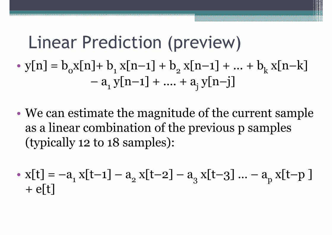
Linear Prediction (preview)

• y[n] = b0x[n]+ b1 x[n–1] + b2 x[n–1] + ... + bk x[n–k] – a y[n–1] + .... + a y[n–j]– a1 y[n–1] + .... + aj y[n–j]

• We can estimate the magnitude of the current sample as a linear combination of the previous p samples (typically 12 to 18 samples):

• x[t] = –a1 x[t–1] – a2 x[t–2] – a3 x[t–3] … – ap x[t–p ] + e[t]

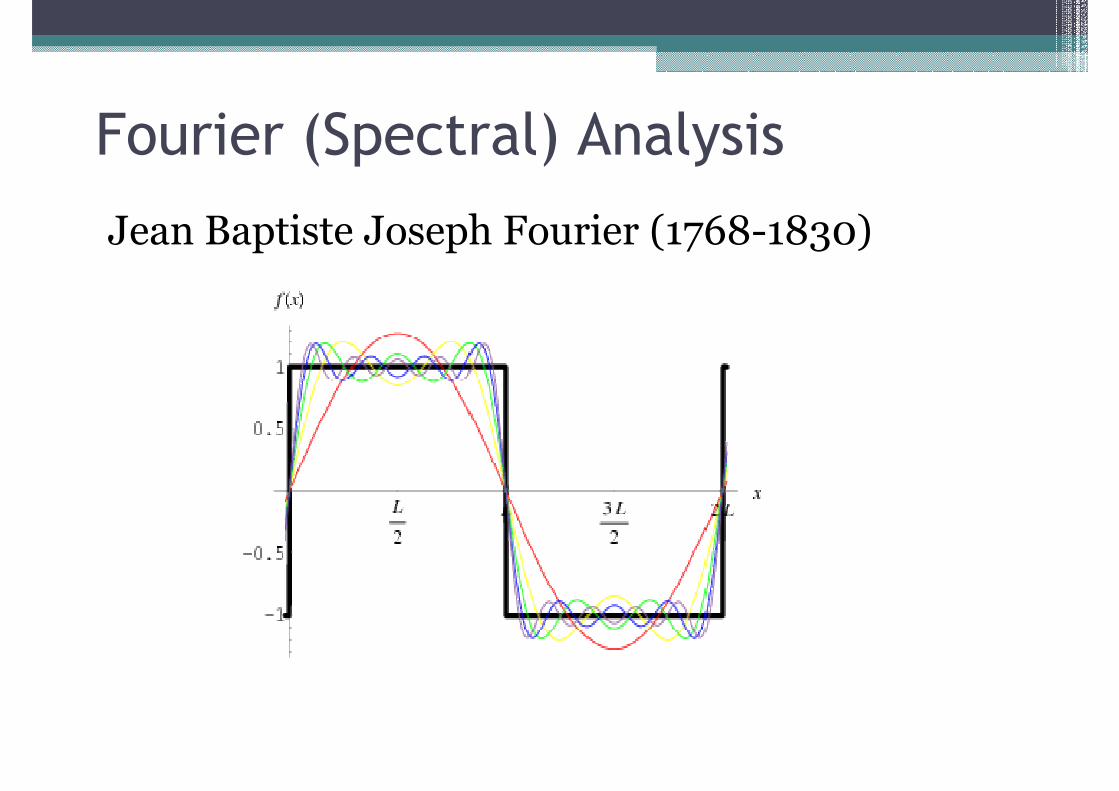
Fourier (Spectral) Analysis

Jean Baptiste Joseph Fourier (1768-1830)

Windowing

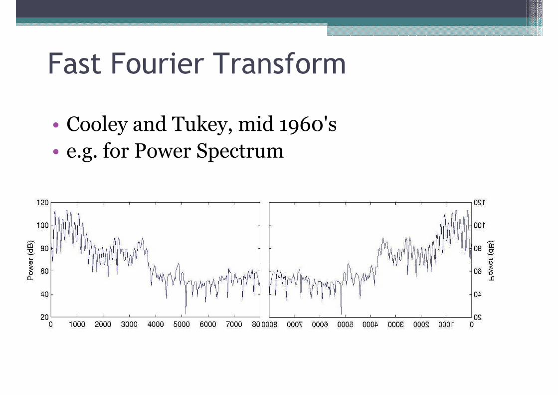
Fast Fourier Transform

• Cooley and Tukey, mid 1960's• Cooley and Tukey, mid 1960's• e.g. for Power Spectrum

Fast Fourier Transform

• Cooley and Tukey, mid 1960's• Cooley and Tukey, mid 1960's• e.g. for Power Spectrum

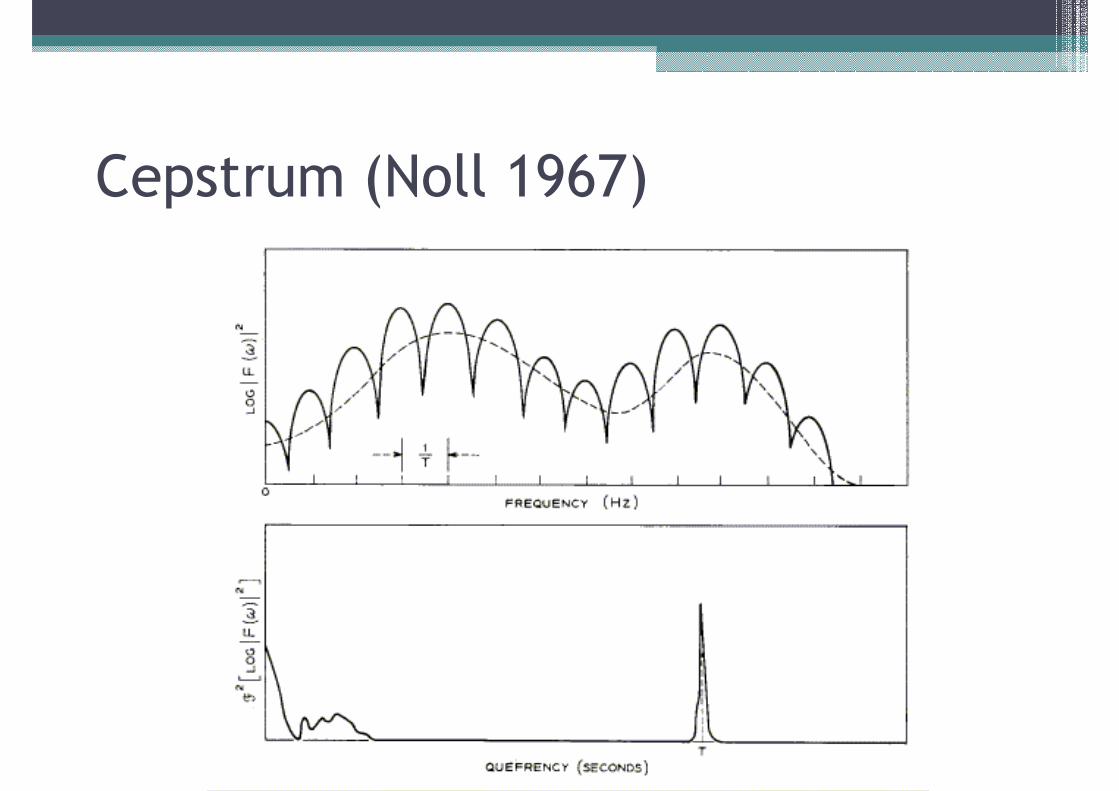
Cepstrum (Noll 1967)

Cepstrum

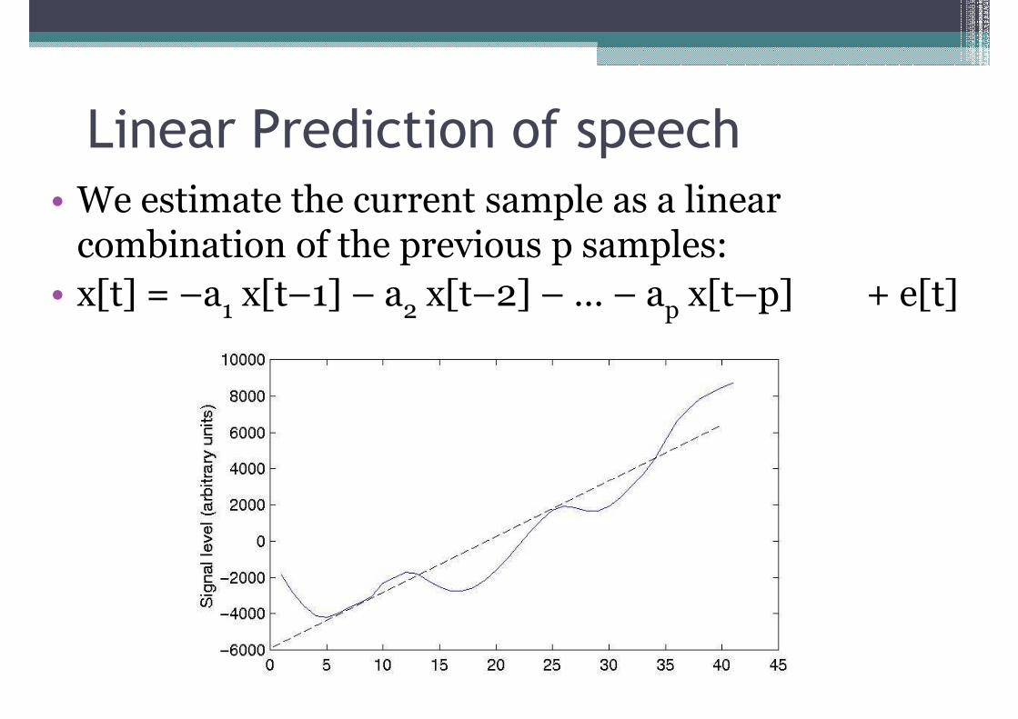
Linear Prediction of speech

• We estimate the current sample as a linear combination of the previous p samples:combination of the previous p samples:

• x[t] = –a1 x[t–1] – a2 x[t–2] – … – ap x[t–p] + e[t]

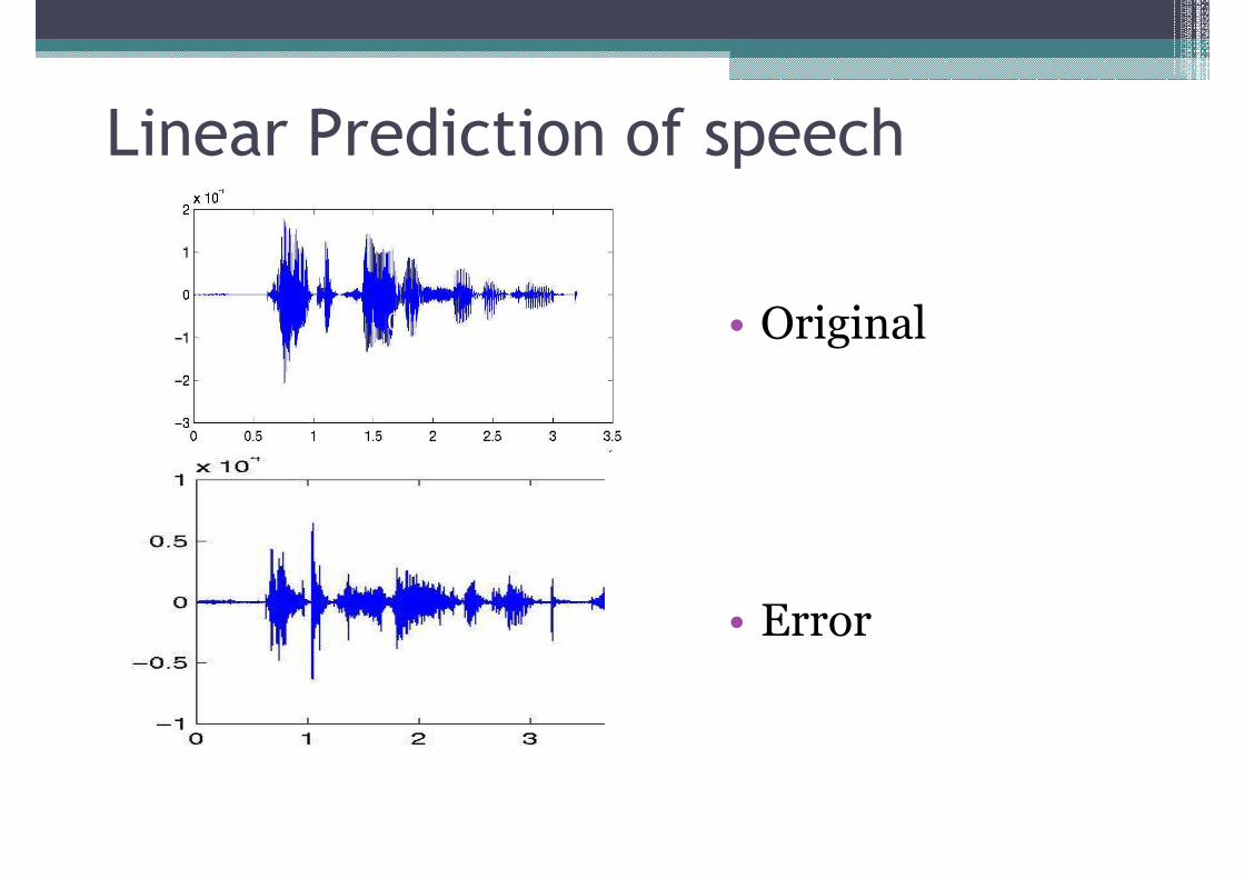
Linear Prediction of speech

0 • Original

• Error

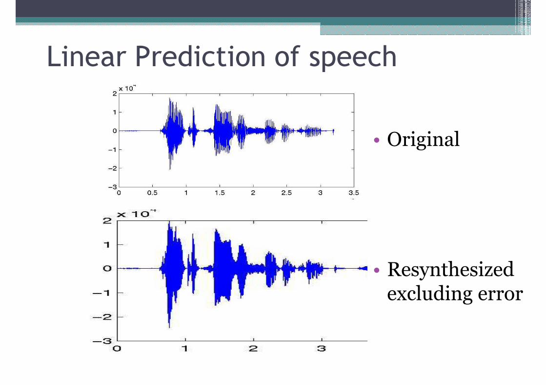
Linear Prediction of speech

• Original0 • Original

• Resynthesized excluding error

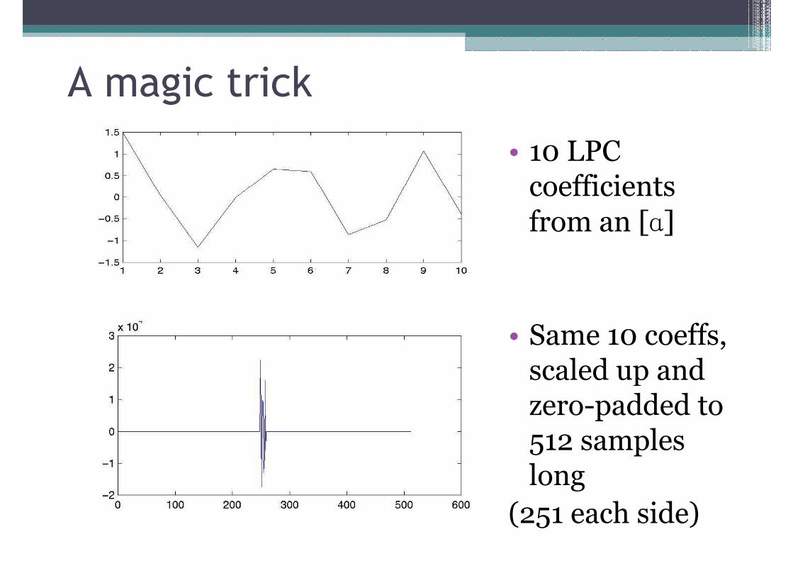
A magic trick

• 10 LPC coefficients coefficients from an [ɑ]

• Same 10 coeffs, scaled up and scaled up and zero-padded to 512 samples long

(251 each side)

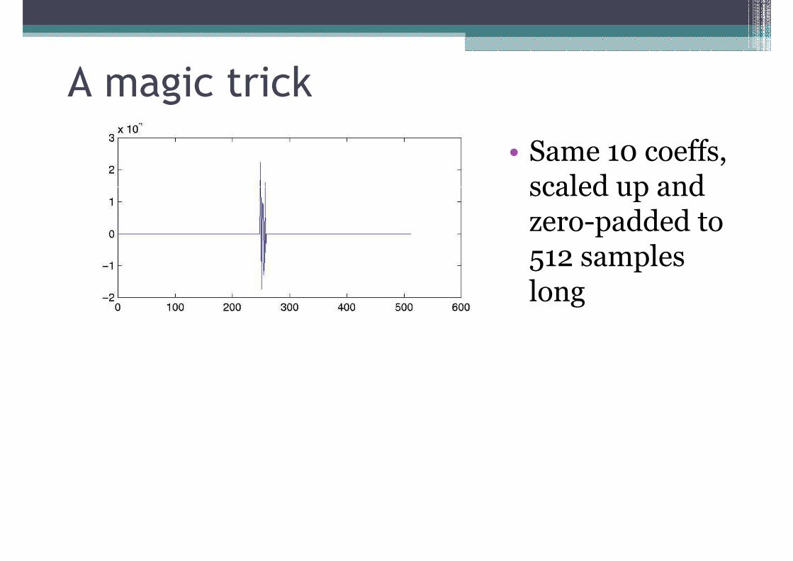
A magic trick

• Same 10 coeffs, scaled up and scaled up and zero-padded to 512 samples long

A magic trick

FFT

LPspectrum

FFT

F1 F2

F3 F4

Shameless plug