jochen triesch, uc san diego, triesch 1 local stability analysis step one: find stationary point(s)...

Jochen Triesch, UC San Diego, http://cogsci.ucsd.edu/~triesch 1

Local Stability AnalysisLocal Stability Analysis

Step One: find stationary point(s)

Step Two: linearize around all stationary points (using Taylor expansion),the Eigenvalues of the linearized problem determine nature of stationary point:

Real parts: positive: growth of fluctuations, instability negative: decay of fluctuations, stability

Imaginary parts: if present, solutions are oscillatory (spiraling) spiraling inward or outward if non-zero real parts

Overall: point (asymptotically) stable if all real parts negative


Examples of nonlinear activation functions (transfer functions):

a.b.c.

c. rectified hyperbolic tangent

LLg

rLF

2/11

max

exp1

b. “sigmoidal function”

02max tanh LLgrLF

else:0

0:0

LLLLGLF

a. “half-wave rectification”

Note: we will typically consider theactivation function as a fixed propertyof our model neurons but real neuronscan change their intrinsic properties.


The Naka-Rushton function

P ½ , the “semi-saturation”, is the stimulus contrast (intensity) that produces half ofthe maximum firing rate rmax. N determines the slope of the non-linearity at P ½ .

else:0

0:2/1

max PPP

PrPF NN

N

A good fit for the steady state firing rate of neurons in several visual areas (LGN,V1, middle temporal) in response to a visual stimulus of contrast P is given by:

Albrecht andHamilton (1982)


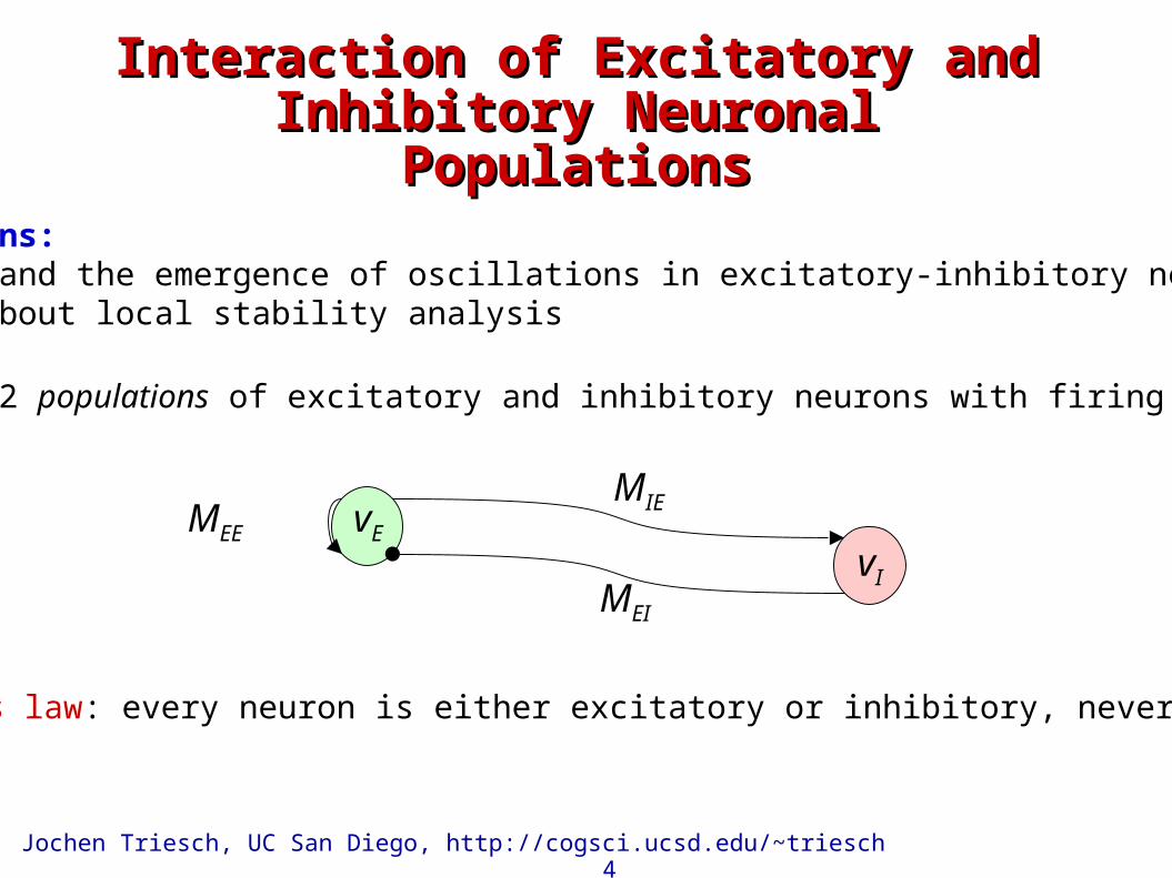
Interaction of Excitatory and Inhibitory Interaction of Excitatory and Inhibitory Neuronal PopulationsNeuronal Populations

MEE vE

MIE

MEI

Dale’s law: every neuron is either excitatory or inhibitory, never both

Motivations:• understand the emergence of oscillations in excitatory-inhibitory networks• learn about local stability analysis

Consider 2 populations of excitatory and inhibitory neurons with firing rates v:

vI


Parameters: MEE = 1.25, MEI = -1, gammaE = -10Hz, tauE = 10ms MII = 0, MIE = 1, gammaI = 10 Hz, tauI = varying

MEE

vE vIMIE

MEI

[ ]+

Mathematical formulation:

Stationary point:

67.16 ,67.26 00 IE vv


stationary point *nullclines, zero-isoclines

*

*

Phase PortraitPhase Portrait

A: Stationary point is intersection of the nullclines. Arrows indicate directionof flow in different area of the phase space (state space).

B: real and imaginary part of Eigenvalue as a function of tauI .


Linearization around stationary point givesthe following matrix A with these Eigenvalues:


For tauI below critical value of 40ms, Eigenvalues have negative realparts: we see damped oscillations. Trajectory spirals to stable fixed point


When tauI grows beyond critical value of 40ms, a Hopf bifurcation occurs(here tauI=50ms): stable fixed point → unstable fixed point + limit cycle

Here, the amplitude of the oscillation grows until the non-linearity “clips” it.


Neural OscillationsNeural Oscillations

• interaction of excitatory and inhibitory neuron populations can lead to oscillations

• very important in, e.g. locomotion: rhythmic walking and swimming motions: Central Pattern Generators (CPGs)

• also very important in olfactory system (selective amplification)

• also oscillations in visual system: functional role hotly debated. Proposed as solution to binding problem:

• Idea: neural populations that represent features of the same object synchronize their firing


Binding ProblemBinding Problem• what and where (how) pathways in visual system• how do you know what is where?

circle

triangle

up

downvisual field

neuralrepresentation

Synchronizationno yes

spike trains


Competition and DecisionsCompetition and DecisionsMotivation: ability to decide between alternatives is fundamentalIdea: inhibitory interaction between neuronal populations representing different alternatives is plausible candidate mechanism

The most simple system:

0: 0

0:120

100

31

31

22

2

1222

2111

x

xx

xxS

eKSee

eKSee

Winner-take-all(WTA) network

K1 K2


Stationary States and StabilityStationary States and Stability

222

2

22

2

2

0: 0

0:

x

xM

dx

dS

x

xx

MxxS

The stationary states for K1=K2=120:• e1 = 50, e2 = 0• e2 = 50, e1 = 0• e1 = e2 = 20

Linear stability analysis:1) for e1 = 50, e2 = 0 :

2) for e1 = e2 = 20 : (τ=20ms)

/1 with , 0

01

1

A

03.0 ,13.0 with , 21158

581

A

→ “stable node”

→ “unstable saddle”

12222111 31

, 31

eKSeeeKSee


Matlab SimulationMatlab Simulation

one unit wins the competition and completely suppresses the other

0 50 100 150 200 250 300 350 4000

5

10

15

20

25

30

35

40

45

50

Time (ms)

E1

(red

) &

E2

(blu

e)

0 10 20 30 40 50 600

10

20

30

40

50

60

E1E

2

Plase Plane

Behavior for strong identical input: K1=K2=K=120


Continuous Neural FieldsContinuous Neural FieldsSo far: individual units, with specific connectivity patternsIdea: abstract from individual neurons to continuous fields of neurons, wheresynaptic weights patterns become homogeneous interaction kernels

Variant 1:continuous labeling of input or

output domain

Variant 2:continuous labeling of two-dimensional cortical space


Recurrent Simple Cell ModelRecurrent Simple Cell Model

Question: how is orientation selectivity achieved? (feedforward vs. recurrent accounts)


Classic Hubel and Wiesel ModelClassic Hubel and Wiesel Model

simple cell sums input fromgeniculate On and Off cells in

particular constellation

complex cell sums inputs fromsimple cells with same orientation

but different phase preference


Recurrent ModelRecurrent Model

)'('2cos

')()(

)(10

2/

2/

v

dhv

dt

dvr

2cos1)( AchStimulus with orientation angle θ=0. A: amplitude, c: contrast, ε: small

nonlinear amplification


Superior Colliculus and SaccadesSuperior Colliculus and Saccades

Representation of saccade motor command in superior colliculus: vector averaging

Yarbus


A Simple Model of Saccade A Simple Model of Saccade Target SelectionTarget Selection

noise.: input,: constant, a is , 0

and , 0:0

0:1)(, )2/exp()(

),(),()),(()),(()(),(),(

22

21

2

ηI

h

hhSg

ttIthSthSgthth

xx

xxxxxxx

Question: how do you select the target of your next saccade?Idea: competitive “blob” dynamics in 2 dimensional “neural field”

layer of non-linear units with local excitation

linear unit for global inhibition


Stability Analysis of Saccade ModelStability Analysis of Saccade Model


and , 0:0

0:1)(, )2/exp()(

),(),()),(()),(()(),(),(

22

21

2

ηI

h

hhSg

ttIthSthSgthth

xx

xxxxxxx

Step 1: look for homogeneous stationary solutions

Step 2: find range of β for which homogeneous stationary solution becomes unstable

Step 3: simulate system (Matlab), observe behavior

Step 4: estimate the size of the resulting blob as a function of β

')'()'()()( xdxgxxfxgxf

)()()()( xfxgxgxf

')'()( xdxfxf

Reminder: Convolution

)(F)(F)()(F xgxfxgxf


Example RunExample Run

Initialization: 10 random spots of small activity, I=0, η small Gaussian iid noise

time

Result: a blob of activity forms at location determined by initial state and noise


Results of AnalysisResults of Analysis


and , 0:0

0:1)(, )2/exp()(

),(),()),(()),(()(),(),(

22

21

2

ηI

h

hhSg

ttIthSthSgthth

xx

xxxxxxx

Step 1: look for homogeneous stationary solutions• h0=0 works, β>1/A prevents fully active layer (A=area of layer)

Step 2: find range of β for which homogeneous stationary solution becomes unstable

• for small local fluctuation from h0=0 to grow, we need β<1/2πσ2

Step 3: simulate system (Matlab), observe behavior• formation of single blob of activity suppressing all other activity in layer

Step 4: estimate the size of the resulting blob as a function of β, σ•

rr for , 21


Matlab Code FragmentsMatlab Code Fragments

% initialize layer

size = 50;

h = zeros(size,size);

for i=1:10

x = unidrnd(size);

y = unidrnd(size);

h(x,y)=h(x,y)+0.05;

end

% main loop

while(1)

active = (h>0);

I = conv2(active, g, 'same') - beta*(sum(sum(active)));

h = (1-alpha)*h + alpha*I + normrnd(0, noise, size, size);

% display plots, etc.

pause

end

% initialize layer

size = 50;

h = zeros(size,size);

for i=1:10

x = unidrnd(size);

y = unidrnd(size);

h(x,y)=h(x,y)+0.05;

end

% main loop

while(1)

active = (h>0);

I = conv2(active, g, 'same') - beta*(sum(sum(active)));

h = (1-alpha)*h + alpha*I + normrnd(0, noise, size, size);

% display plots, etc.

pause

end


Discussion of Saccade ModelDiscussion of Saccade Model

Positive:• roughly consistent with anatomy/physiology• explains how several close-by targets can win over strong but isolated target• suggests why time to decision is longer in situations with several equally strong targets• similar models used in modeling human performance in visual search tasks

Limitations:• only qualitative account• in order to make precise quantitative predictions, it is typically necessary to take more physiological details into account, which are mostly unknown:

• exact connectivity patterns• non-linearities• more than one area is involved• what are all the inputs?


Connection to Maximum Connection to Maximum Likelihood EstimationLikelihood Estimation

So far: purely bottom-up view: networks with this connectivity structure just happen to exhibit this behavior and this may be analogous to what the brain doesNew idea: use such dynamics to do Maximum Likelihood estimation

Want:

New idea: blob dynamics + vector decoding works better than doing direct vector decoding on the noisy inputs

1-d “blob” network with noisy input

)|(maxargˆ

rp r: firing rate vector, Θ: stimulus parameter

Population vector decoding:

a

N

a a

a

r

rcv

1

maxpop

where ca is the preferredstimulus vector for unit a


Binocular Rivalry, Bistable PerceptsBinocular Rivalry, Bistable Percepts

Idea:extend WTA network by slowadaptation mechanism. Adaptation acts to increase semi-saturation of Naka Rushton non-linearity

222

111

212

22

212

22

221

21

221

11

)(

)(

eaa

eaa

eKa

eKree

eKa

eKree

A

A

ambiguous figurebinocular rivalry

L R


Matlab SimulationMatlab Simulation

2222

122

2

212

22

111221

21

221

11

, )(

, )(

eaaeKa

eKree

eaaeKa

eKree

A

A

0 10 20 30 40 50 600

10

20

30

40

50

60

A1

E1

E1-A1 Projection of State Space

0 1000 2000 3000 4000 5000 60000

10

20

30

40

50

60

Time (ms)

E1

(red

) &

E2(

blue

)

β=1.5β=1.5


Discussion of Rivalry ModelDiscussion of Rivalry Model

Positive:• roughly consistent with anatomy/physiology• offers parsimonious mechanism for different perceptual switching phenomena, in a sense it “unifies” different phenomena by explaining them with the same mechanism Limitations:• provides only qualitative account• real switching behaviors are not so nice and regular and simple:

• cycles of different durations• temporal asymmetries• rivalry: competition likely takes place in hierarchical network rather than in just one stage.• spatial dimension was ignored

jochen triesch, uc san diego, triesch 1 local stability analysis step one: find stationary point(s)...

Documents

jochen triesch

uc san diego

stable fixed point slide

vivi slide

real parts negative

nature of stationary

real neurons

function of tau