JMP® is statistical discovery software that can help you explore data, fit models, discover patterns, and discover points that don’t fit patterns. As statistical discovery software, the emphasis in JMP is to interactively work on data to find out things.• Using graphics, you are more likely to make discoveries. You are also

more likely to understand the results.

• With interactivity, you are encouraged to dig deeper, for one analysis can lead to a refinement, one discovery can lead to another discovery; and you can experiment with statistics to improve your chances of discovering something important.

• With a progressive structure, you build context that maintains a live analysis, so you don’t have to redo analyses, so that details come to attention at the right time.

JMP IN, a student version of JMP, is distributed by Duxbury Press.

JMP is statistical software that gives you an extraordinary graphical interface to display and analyze data. JMP is for interactive statistical graphics and includes:• a spreadsheet for viewing, editing and manipulating data• a broad range of graphical and statistical methods for data analysis

• an extensive design of experiments module

• options to highlight and display subsets of the data

• data management tools for sorting and combining tables

• a calculator for each table column to compute values

• a facility for grouping data and computing summary statistics

• special plots, charts and communication capabilities for quality improvement

• tools for moving analysis results between applications and for printing

• a scripting language for saving frequently used routines

OBJECTIVES

Start JMP softwareOpen a JMP data tableIdentify key data table features

• To begin using JMP software, double click on the icon corresponding to either

• the JMP application

or• a JMP data table

The program opens with a brief animation and soon after a standard application window with standard Windows features and controls and the a new Tip of the Day

From the JMP Starter File Menu: From the JMP menu bar:

Now browse the folder and select the JMP data file and click “open”

From the JMP File menu bar select Preferences,

or in the JMP Starter window click on

These choices in the preferences allow you to tailor things such as:

general operation and appearance of JMP

background color of windows and graphs

type, style, and size of fonts

graphic formats for copy and drag results and RTF and HTML files

communications settings

default directory paths for file locations

results initially presented by each analysis or graph platform.

settings for importing and exporting data to suit your needs or situation.

Now let us activate the Laser Pointer in the “Reports” option under the Preferences.

The Laser Pointer is now active and you can use it when you point the figures in the JMP output as shown below.

21

22

Example: The data are stored in the ARsoils.jmp data table.

To open the ARsoils.jmp data table selectOpen Data Table from the JMP starterSelect ARsoils.jmp from the “appropriate subdirectory”.

23MORE ON PANELS AND DATA TABLE CURSOR FORMS…

The data table is the entire window. It contains • the data grid on the right and• three information panels on the left

• one for the table • one for the columns • one for the rows

The rows and columns panels give corresponding counts.

To hide or unhide the three left panels click on the blue diamond located on the upper-left corner of the data grid. This data table has • 30 columns (variables) and • 120 row (observations)

24

The data type of a column determines the way the data can be used. JMP uses two primary data types:

Numeric:Columns with numbers that can be used in calculations. These data are right-aligned.(see Depth or BD).

Character:Columns with numeric and/or character values that can be used to designate different levels of the variable. These data are left-aligned.(see Soils).

The modeling type of a column determines how the data are used in an analysis.

Three modeling types used in JMP:

Continuous: For numeric data whose values are used directly in computations (for example, BD).

Ordinal: For numeric and/or character data used to group the observations into a set of levels with an inherent order (for example Depth).

Nominal: For numeric and/or character data used to group the observations into a set of levels without any inherent order (for example, MLRA).

26

To specify or see the modeling type of a variable:

Right-click on the column heading and choose

Column info... from the given options. Or, simply double click on the column title.

A new window will open showing the column specifications.

Discuss current properties, row states and much more here…

27

The column role identifies the role of the column in an analysis. Four column roles used by JMP are:

X the column stores values for the independent or predictor variable

Y the column stores values for the dependent or response variable

Weight the values for the column represent the weight for each row

Freq the values for the column represent the frequency for each row

If no specific role is identified for the variable, use the “No Role” option.

MORE ON LABELS etc

28

To specify the column role of a variable: Right-click on the column

heading. Choose Preselect Role from the given options. Specify a role from the drop-down menu.

More on consequences on Preselecting Column Roles …

29

After selecting a row (column):• Press the Shift key to select a block of adjacent rows (columns)• Press the Ctrl key to select nonadjacent rows (columns)Note: The ALT key is the OPTION key...

Click on the area or box marked1: to select a row2: to select a column 3: to deselect all selected rows 4: to deselect all columns 5: to edit a cell6: to change the modeling type7: to edit the variable column information (column name, data and modeling type, format, etc.) double click

1

34

257

6

30

File performs most routine file functions, such as opening, closing, and saving

Edit performs most common editing functions such as cutting and pasting

Tables performs table functions, such as sort, subset, and merge

Rows performs row operations (recall that JMP treats rows as observations)

Cols performs column operations(recall that JMP treats columns as variables)

DOE facilitates the Design Of the Experiment

31

Analyze performs most statistical analyses

Graph generates a variety of plots

Tools displays analysis window tools

View appears only under the Windows operating system environment

Window selects among currently opened windows and performs window operations

Help accesses the main help features in JMP

32

• Builds the new data table, new script window, new project and new Journal• opens an existing JMP data table• closes the current JMP data table• Writes an open text file to a JMP data table• saves the current data table• removes all changes to data table since you last saved it• links to data base at a different location• Lets you open an internet browser within JMP• selects default preferences• printing options• previews ready to print window• selects desired print format• location and name of the data table(s) used (1 is most current)• Saves the script of the executed analysis.• Saves the executed analysis and data table as a Project• exits JMP software

33

• undoes the last action if possible• redoes last action if possible• cuts selection and keeps it in clipboard• copies selection• copies selection only in text format• Preserves the data table's column labels in the copied image• pastes data • Uses the first line of information on the clipboard as column headers• clears the data at the end of the current data table• selects all data in data table• saves selection in desired format• runs script if there is one in the current window• Submits the JMP scripts as a SAS program to SAS server

Gives you the ability to find and replace text in data tables and scripts

Finds the line in the data table for observations that meet your criteria

Saves a report just as it appears in the report window

Lets you edit or manipulate the report before you save

Reveals a submenu to customize menus and toolbars. Revert to Factory Defaults resets the menus and toolbars to the arrangement when you first installed JMP

35

request summary statistics by grouping columns subset selected rows. Random sampling available. sort rows by specified columns. stack values from several columns into several rows in one column. split a column, mapping several rows on one column to one row in several columns. interchange rows and columns. combine rows from several sources. join rows from several sources by matching value a table Tabulate- To build table using two option, interactive or dialog. Missing Data Patterns- To find the patterns of missing values in the data and make a table of each pattern and its frequency.

36

Recall that JMP treats rows as observations.

excludes or includes an observation in statistical analyses

hide or unhide an observation in point plots labels or unable an observation in point plots lists colors lists markers searches for observations meeting your criteria returns to last selection utilities on row selection undoes all row selection assigns colors or markers to rows brings up a window useful for browsing all cols for

each row adds new rows (default=20) moves selected rows (default=To End) deletes selected rows Lets you select rows, create subsets and animate

selected rows

37

Recall that JMP treats columns as variables creates a new column lets you add more than one column at a time Highlights a specific column in the table opens the column info for a selected column lets you assign the most common analysis roles lets you define values using some formula lets you enter a list of valid values or range limit

conditions use this column’s values to identify points in plots locks column into left-most position in the data grid hides columns from view excludes variable in analysis role assignment dialogs modifies the attributes of selected columns lets you move columns by several options deletes selected columns Lets you quickly recode data that is coded

incorrectly

38

The Design of Analysis menu launches statistical platforms. Create a design tailored to meet specific requirements. Sift through many factors to find the few that have the

most effect. Find the best response allowing quadratic effects

(curvature). Generate all possible combinations of the specified factor

settings. Lets you define a set of factors that are ingredients in a

mixture Creates a design by spreading the design points out to the

maximum distance possible between two points Lets you create an optimal design for models that are

nonlinear in the parameters. Make inner and outer arrays from signal and noise

factors. Optimize a recipe for a mixture of several ingredients.

Add more runs to an existing data table. Replicate, add center points, fold over or add model terms.

Plot any two of the power to detect an effect, the sample size, and the effect size given the third. Or, compute one given the other two.

39

The Analyze menu launches statistical platforms.

• investigates the distribution of values in each column• investigates all types of “pairwise relationships and analysis” • models one or more response variables with one or more predictor variables• allows for the creation of a model specific for the data • performs nonlinear regression, time series analysis and neural nets analysis• explores how multiple variables relate to each other, and how points fit that relationship, cluster and discriminant analysis • performs survival analysis

40

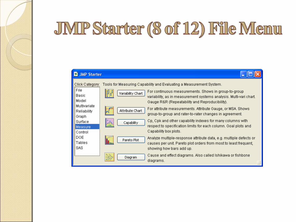
The Graph menu generates a variety of graphs.

• produces bar and pie charts• produces overlay plots• Scatterplot 3D produces a three-dimensional rotatable display of values from any three numeric columns in the active data table• produces contour plots • Bubble Plot is a scatter plot which represents its points as circles (bubbles)• The Parallel Plot command draws a parallel coordinate plot• Produces a rectangular array of cells drawn with a one-to-one correspondence to data table values• The Tree Map command displays tree maps• The Scatterplot Matrix command allows quick production of scatterplot matrices• The Ternary Plot command constructs a plot using triangular coordinates• The Diagram platform is used to construct Ishikawa charts, also called fishbone charts, or cause-and-effect diagrams

• produces statistical quality control plots• Variability or Continuous Gage charts are for

responses whose values can be measured on a continuous scale. Attribute Gauge charts are for responses whose values are binary or categorical

• produces Pareto charts• Capability analysis, used in quality control,

measures the conformance of a process to given specification limits.

• The Profiler is available for tables with columns whose values are computed from model prediction formulas

• The Contour Profiler command works the same as the Profiler command

• The Surface Plot command plots surfaces and points in three dimensions based on formulas or data

• The Custom Profiler command is available for tables with columns whose values are computed from model prediction formulas.

41

42

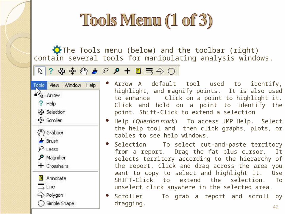
Arrow A default tool used to identify, highlight, and magnify points. It is also used to enhance Click on a point to highlight it. Click and hold on a point to identify the point. Shift-Click to extend a selection

Help (Question mark) To access JMP Help. Select the help tool and then click graphs, plots, or tables to see help windows.

Selection To select cut-and-paste territory from a report. Drag the fat plus cursor. It selects territory according to the hierarchy of the report. Click and drag across the area you want to copy to select and highlight it. Use SHIFT-Click to extend the selection. To unselect click anywhere in the selected area.

Scroller To grab a report and scroll by dragging.

The Tools menu (below) and the toolbar (right) contain several tools for manipulating analysis windows.

43

Grabber (Hand) To direct manipulation in plots and charts, e.g., change the # of bars in a histogram or to shift the boundaries of the bars on the axis, to spin a spinning plot,or to rearrange a scatterplot matrix.

Brush Click and drag with the Brush to highlight selection. Use alt-click to change the size of the brush rectangle. Use shift-click to extend a selection.

Lasso Click and drag with the Lasso tool to highlight the selection.

Magnifier To zoom in on any area of a plot. The click-point becomes the center of a new view of the data. (Alt-Click to restore the original plot.)

Crosshairs A movable set of axes to measure points and distances in graphical displays. Useful on a fitted line or curve to identify the response (“Y”) value for any given value of “X”.

The Tools menu (below) and the toolbar (right) contain several tools for manipulating analysis windows (discussed in that order below)

44

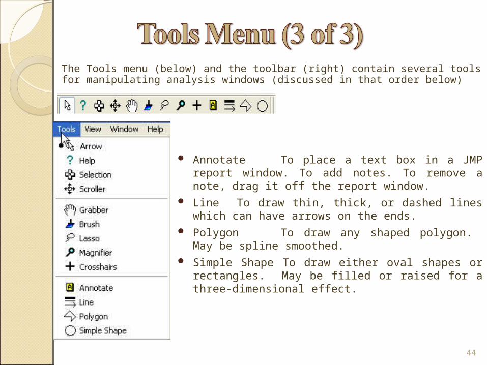
The Tools menu (below) and the toolbar (right) contain several tools for manipulating analysis windows (discussed in that order below)

Annotate To place a text box in a JMP report window. To add notes. To remove a note, drag it off the report window.

Line To draw thin, thick, or dashed lines which can have arrows on the ends.

Polygon To draw any shaped polygon. May be spline smoothed.

Simple Shape To draw either oval shapes or rectangles. May be filled or raised for a three-dimensional effect.

45

JMP Starter Opens the JMP Starter Window. Window List The Window List command displays a

pane at the left side of the JMP window that lists the name of each window you have open in JMP

File System The File System command displays a pane at the left side of the JMP window that shows your PC's file system

Projects The File System command displays a pane at the left side of the JMP window that lists all open projects.

The View menu appear only under the Windows operating system environment.

Log Displays a pane that monitors JSL statements as they execute. (The log window is editable.)

Show Toolbars Lists all available toolbars with a check box to hide or reveal them.

Float Log To detach or re-attach the log window to the bottom of the screen, right-click Log and select Float Log Window

Status Bar Turns the Windows status bar on or off at the bottom window edge.

46

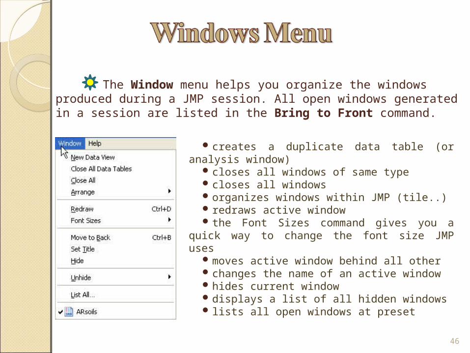
The Window menu helps you organize the windows produced during a JMP session. All open windows generated in a session are listed in the Bring to Front command.

creates a duplicate data table (or analysis window)closes all windows of same typecloses all windowsorganizes windows within JMP (tile..)redraws active window the Font Sizes command gives you a quick way to

change the font size JMP usesmoves active window behind all otherchanges the name of an active windowhides current window displays a list of all hidden windowslists all open windows at preset

47

To access the main help features from the help menu in JMP.

Select Help Contents to obtain the main help reference.

Inspect the help dialog.

48

For example, to access help on the topic of neural nets:Select Help Index type Neural Net and double click on Neural Net from the index list.

49

Edit the data table Inspect and edit column information Use list check and range check validation. Transforming data (Create new variables) Sorting the data. Creating subsets of the data. Creating and plotting summary statistics BY-Group Analysis More EDA using Arsoils2.jmp to explore

various objectives and demonstrate analysis and graphs features.

OBJECTIVES

50

Inspect the ARsoils.jmp file. Let’s utilize “Standardize Columns Attributes” to appropriately place the units information which is presently included as part of the Ksat variable names.

51

Now let’s edit the variables of both Ksat columns by taking out the units from the names and editing the Notes placeholder for the Ksat-geo to reflect that it is a geometric and not an arithmetic mean.

Select both Ksat variables. (if not already selected)

Select Cols Column Info…and delete the (cm/hr) from both Column names OR right-click on each column heading then select Column Info

Select Column Properties Notes and edit the notes box for Ksat-geo

Select OK

52

Now let us edit the variables of both “Ksat-” columns by taking out the units from the names and editing the Notes placeholder for the Ksat-geo to reflect that it is a geometric and not an arithmetic mean again.

Select both Ksat variables. (if not selected)

Option click (right hand mouse) Standardize Attributes …

Under Format Best select Fixed Dec

Change the default from 0 decimals to 4 in the Dec: area for that format Select OK Save the data as ARsoils1.jmp select File Save As…

53

Column names can be up to 31 characters long and can consist of any combination of letters and numbers, as well as special symbols (and a blank(s)).

Change the name of the MLRA column to Major Land Resource Areas.

1.Click once on the column heading (selects the column) for MLRA in the column panel.

2.Click again on your selected word MLRA to edit it.

3.Type Major Land Resource Areas.

4.You can adjust the column width if necessary by placing the cursor over the dividing line on the right side of the column you want to widen. As the cursor moves over the line, it changes from an arrow to a double-arrow.

5.Change the name back to MLRA.

54

JMP software has a graphical user interface (GUI). The cursor changes when it passes over certain areas of a data table. Depending on the data table, you most commonly seeThe cursor is the standard arrow when it is in the panels area to the left of the data table, in the triangular rows and columns area in the upper-left corner of the data grid, or on the title bar of the tables panel

When the cursor is within a column heading or a row number area, it becomes a large plus, indicating it is available to select rows or columns

When you select editable text, the cursor becomes a standard I-beam

The cursor changes to a double arrow when it is on a column boundary

when the cursor is over a column with list check validation

when the cursor is over a column with range check validation

The cursor changes to a pointer over any red triangle icon or diamond-shaped disclosure button

55

Data validation enables you to set up a table of acceptable values or range of values for a column. JMP supports two types of validation accessible through the Column Info… dialog.

List check is commonly used for character variables to ensure all values entered for a column correspond to values in a validated list.

Range check is available only for numeric variables to ensure all values entered are within a specified range of values.

Close the Column Info… dialog and return to the data table.Move the cursor over the desired column panel. Right Click and then select validation in the drop down list. Which columns are employing validation? Answer: BD (is range checked) and Texture class (is list checked).

56

Create new variables from existing ones to facilitate the analysis

Use the Formula editor to create and change formulas that create the column values

OBJECTIVES

57

First let us inspect the last variable in the column panel. The next to a column name indicates that this column is created by the Formula

Editor. To view the formula that created the column:1. Select lksat-g by clicking it the column panel.2. Right-click the selected column, and see that Formula… is checked.3. Select Formula and you see that the variable is created to be the natural logarithm

(Log10 is used for log base 10) of the ksat-geo variable.

58

Let’s create a new variable that is the natural logarithm of Ksat-arit.

1. Select Cols New Column…2. Note the defaults (Name, Data & Modeling

Type…) in the New Column window. 3. Select Column Property Formula. (See how

the Formula Editor window opens.)

4. Select Transcendental Log5. Select Ksat-arit (from the Table Columns).

Note that it appears in the box as shown at the right.

6. Select OK to close the Formula box. 7. Select OK to close the New Column. 8. To delete the new Column 31 option, select it

and click on Delete Columns.

59

Say we are interested in creating as a new column the sum of the Sand, Silt and Clay variables. We want the new variable to be the total of the three variables and give it a Format with 0 decimals. Does the new variable contain the value of 100 for all observations? Hint: One can use several ways to accomplish this task three of which are sketched below.

Method 1: Highlight to select the three variables one at a time from the Column variables and click the plus in between selections. Your formula should look “like the one below” before you click Apply sand + silt + clay Select the outside box that contains the above expression and press the delete Key, or simply click on the Clear button.

Method 2: Double click inside the no formula and using your keyboard type the above expression and then click Apply (you should see the same formula in the box as before)

Select the outside box that contains the above expression and press the delete Key, or simply click on the Clear button.

Method 3: From the Functions menu select Statistical Sum (press the comma from your keyboard twice to create two commas that will receive each of the three variables from the Table Columns that now reads Sum(sand,silt,clay). Click Apply.

Delete the new variable when you are finished.

MORE on boxing and a tour of the functions in the Formula Editor…

61

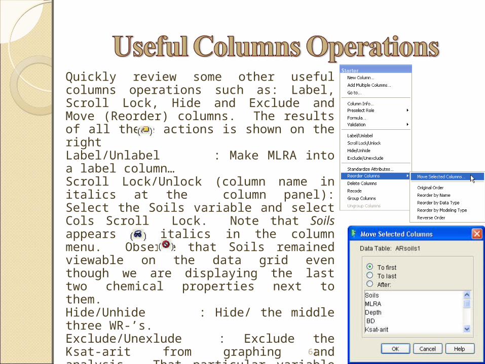
Quickly review some other useful columns operations such as: Label, Scroll Lock, Hide and Exclude and Move (Reorder) columns. The results of all these actions is shown on the right Label/Unlabel : Make MLRA into a label column…Scroll Lock/Unlock (column name in italics at the column panel): Select the Soils variable and select Cols Scroll Lock. Note that Soils appears in italics in the column menu. Observe that Soils remained viewable on the data grid even though we are displaying the last two chemical properties next to them.Hide/Unhide : Hide/ the middle three WR-’s.Exclude/Unexlude : Exclude the Ksat-arit from graphing and analysis. That particular variable and the top surface observations are seen as been excluded from consideration ….Reorder Columns: Select the variable you want to move and right click on it, then choose REORDER COLUMNS from the Drop down list and then select MOVE SELECTED COLUMNS….

62

There are several ways to select rows (observations):

Click in the left margin next to the row number.

Click at the start of the selection and drag to the opposite end.

Click at the start of the selection and shift‑click at the opposite end.

Control‑click to extend the selection without including rows in between.

Control‑click to deselect a row.

Use the Row Selection command in the Rows menu and the Select Where... option to select rows that meet a criterion or a set of criteria.

The same operations are used to select columns (variables) as well.

63

Quickly review the rows panel to see the top surface observations for each of the 12 soils are marked as excluded and that each observation from a given soil has its own color and marker assigned (that are used in all graphs…). You can do to rows some other useful operations similar to the columns operations discussed in the previous slide such as: Label, Hide and Exclude. We will concentrate here on Colors, Markers, and Color or Mark by Column to review how we assigned the row states in the Arsoils1.jmp.The results of all these actions are shown on the right (either from the Rows panel or the Rows menu).1.Select Rows Clear Row States

Now to get it back the way it was:• Select Rows Color or Mark by Column.• Select Soils.• Mark the box Set Marker by Value (as shown).• Select OK.• To save all changes to the row states of ARsoils2.jmp:• Select File Save as…ARsoils2.jmpNote: This will be used in the rest of the slides unless

otherwise indicated.

64

Usually one can obtain a great deal of information by sorting the data.If, for example, you are primarily interested in all the data from MLRA “116” (NWA),1.Select Tables Sort ( Fill the entries as shown below by clicking on the column names in the appropriate order.) 2.Select Sort. In the resulting data table (“Untitled”), MLRA=“116” appears first since by default the sort works in ascending order.Now click and drag the mouse to select the first 10 observations (Soils=Captina). 1.Select Tables Subset 2.Click OK

65

Suppose that we are interested in the following subset of the data that meets ALL three criteria.

a)Texture class contains “l” for “loam”,

b)Acidic pH samples (pH<5)

c)With Iron greater than 100 (Fe>100)

1. Use Rows Row Selection Select Where…

2. Select Texture Class from the drop down list

3. Select the condition “equals” from the drop down list

4. Enter “I” in the adjacent field

5. Click on “Add condition” which will show you “Texture class equals I”

6. Click “OK”

66

To calculate and tabulate the median and range values for NO3, P and K for each soil.1. Select Tables Summary.

2. Click OK. Summary statistics will appear in a new spreadsheet

3. Double click on Source to get Table property window

The Data Filter command in the Rows menu gives a variety of ways to identify subsets of data Using Data Filter commands and options, you interactively select complex subsets of data, hide these subsets in plots, or exclude them from the analyses.

Select Rows Data Filter To use the Data Filter, select one or more variables (Here it is texture class)

in the Add Filter Columns list whose values you want to use as filters and click Add.

67

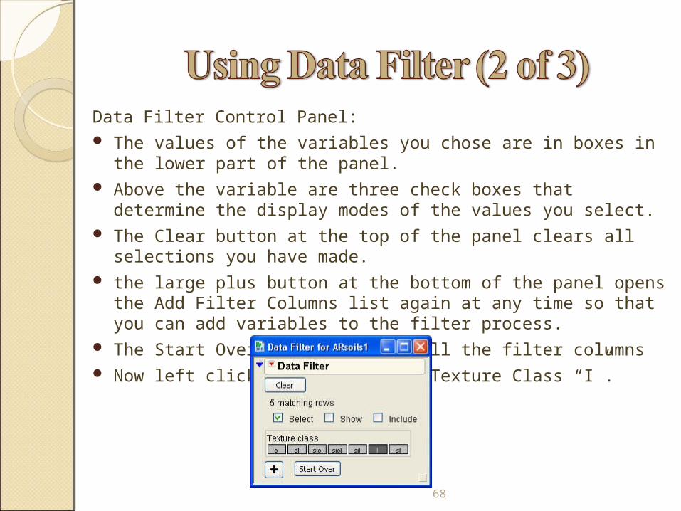
Data Filter Control Panel: The values of the variables you chose are in boxes in the lower part of the panel. Above the variable are three check boxes that determine the display modes of the

values you select. The Clear button at the top of the panel clears all selections you have made. the large plus button at the bottom of the panel opens the Add Filter Columns list

again at any time so that you can add variables to the filter process. The Start Over button removes all the filter columns Now left click on the value of Texture Class “I”.

68

Now click on the plus button at the bottom of the panel to add variable pH to the filter.

Now to select the all the observations less 5 on pH, Shift + click on the right side less or equal to symbol to get < sign.

Similarly, to add the variable Fe >100, click + button at the bottom and in the list of variables select Fe. Now to select the observations greater than 100, Shift + Click on the left side less than or equal to symbol to get <.

70

To calculate the means Ph levels and test for equality of the mean Ph levels for different soil types -- especially to compare “Bowie’s” pH with the other soils’ pH.

One-way ANOVA Fisher’s LSD

Analyze Fit Y by X

Click OK to get the plot. To choose other options, click on the red triangle.

71

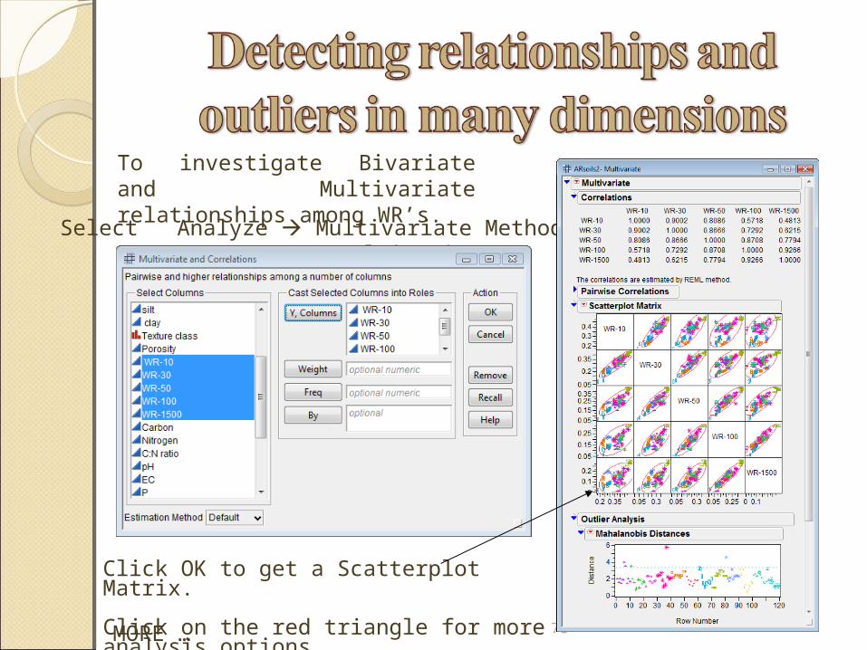
To investigate Bivariate and Multivariate relationships among WR’s.

MORE …

Select Analyze Multivariate Methods Multivariate

Click OK to get a Scatterplot Matrix.

Click on the red triangle for more analysis options.

72

To investigate the relationship of Texture Class to Soils.

Click OK

MORE …

Analyze Fit Y by X

73

To investigate the relationship of Nitrogen to Carbon for four selected soils (MLRA=“134”) (Note: Use the data table CNdata.jmp.)Analyze Fit Y by X

Nitrogen Y, Response and Carbon X, Factor OK

Click on the red triangle by Bivariate… and select Group By… SoilsClick on the red triangle by Bivariate…again and select Fit Line

Discuss the details for customizing getting the graph printed or pasted

OK

74

Distribution is a powerful Exploration tool. To demonstrate, use the general soil texture and composition of the Captina soil found in NWA. Select Analyze Distribution

OK

And after you Click on Captina (to select it) …

75

To get the detailed distribution of Na for each soil across the soil profile: Analyze Fit Y by X

Click OK to get distributions. Click on red triangle for more analysis options.

76

To determine if the the mean Ksat-arit is significantly greater than the mean Ksat-geo overall.

Click OK to get

Good place here to use the magnifier tool …(and ALT to return…)

Note the “unsualy high” difference in the two Ksat values for Row 11

Analyze Matched Pairs

77

To review the relationship of Water Retention (WR’s) to Depth at different pressures for each soil:

MORE…

OK

Graph Chart Choose Data.

Choose line chart

78

To review the “pH Process” (for stability, consistency) over consecutive batches, create a Control Chart (Shewhart) of pH for every “Batch” (10 consecutive samples) from the same soil.

MORE…

OK

Graph Control Chart

79

To study amounts of NO3, P, and K across the profile for each soil:

MORE…

OK

Graph Variability Chart

80

To examine for differences in Texture class for each soil by MLRA:

OK

Part of output shown here. Show how to use Layout to customize…

Graph Pareto Plot

81

To examine for differences Texture class for each soil by MLRA.

OK

Note only the first level (Bowie) of the BY group shown… Take time here to show how to save the script into the data table…

Graph Ternary Plot

82

To summarize and get the means for sand, silt & clay with respect to each soil and MLRA

Tables Tabulate

Drag and drop “MLRA” into “Drop Zone for rows”

Drag and drop “Mean” into “N” to replace N with Mean

83

• Drag and drop “Soils” after “MLRA”

• Drag and drop “sand” under “Mean”

• Drag and drop “silt” under “sand”

• Drag and drop “clay” under “silt”

• To show a graph which goes hand-in-hand with the table

• Click the Platform Menu

• Select “Show Graph”

• To make the created table into a data table

• Click the Platform Menu

• Select “Make Into Data Table”

84

• Graph builder functionality allows you make a graph in just few drag and drops. We could say Graph Builder is Graphical Version of Tabulate function.

• Open ARsoils

• To Launch the Graph Builder Platform

• Click “Graph” Menu “Graph Builder”

• To visualize how the Bulk Density (BD) change over Depths for different soils,

• Drag and Drop “Depth” in X

• Drag and Drop “BD” in Y

• Drag and Drop “Soils” in Wrap

• To add a smoother to the graph

85

• Bubble Plot allows you to Visualize your data in more than 3 dimensional Space.

• Open ARSoils.jmp

• To Launch a Bubble plot platform,

• Click “Graph” Menu “Bubble Plot”

• Provide variables as shown below to make a bubble plot & click OK.

• Click “Go” to visualize the data.

• To Save it as a flash movie

• Click on the platform menu

• Click “Save as Flash (*.SWF)

86

Scripting is considered an advanced feature that is not for novice users. The principal needs that scripting addresses are:

production jobs - when you are doing the same sequence of work repeatedly. customization - when JMP doesn't have a built-in feature and you need to program it packaging - when you need to create a new user interface to do a set of things. data manipulation - when you need to manipulate data in complex ways simulation - when students and researchers need to simulate statistical processes. record keeping - when you want to save the commands for how you analyzed something. customization of graphs - you can put scripting code inside of graphs that executes each time the graph is drawn to overlay additional graphic elements.

87

Illustrate the use of scripts by executing various scripts in the Table panel of ARsoils.jmp.1. Select Ternary Plot in the column window and left click on the red diamond

and select Edit to view the Script for the ternary plot2. Select Ternary Plot in the column window and left click on the red diamond

and select Run Script.

Demonstrate the use of scripts by running the OnewayLines.JSL script to create letters and annotate the Fit Y by X output (see slide 59).

If time permits demo two more scripts…

Test_for_correlated_variances_comparison.jsl tests using Dr. Meullenet sensory data.

Run the vbball.jsl script that creates visual summary basketball statistics.

88

A JMP script is an concise set of instructions that you can use to achieve the same results you achieve when you issue a series of interactive commands. A JMP script conveniently performs otherwise tedious work, provides a record and documentation for review, and alleviates unintentional deviations. You can easily and quickly repeat analyses using a script. Scripts can be saved to the data table, script window, or file. You can attach scripts to the Toolbar with a user‑specified button or to the users menu.  

Scripts are used to extend existing JMP capabilities or to create entirely new capabilities as seen in the two cases on the previous slide. Finally, live demonstrations (as in vbball) and animated results can be created using JMP scripts.

89

JMP software stores information in a data table. For purposes of analysis, JMP views each row as a single observation and each column as a single variable.

Date type is indicated by the alignment of data within a column. Numeric variables (numeric values that can be used in calculations) are right-aligned. Character variables (numeric and/or character values that designate different levels of a variable) are left-aligned. Modeling type is included to the left of each variable name in the Column panel.

You can access, edit and change each variable’s information through the Column Info… dialog. Select the variable and click on Cols¸Column Info... From the Column Info… dialog, you can change a variable’s name, data type, and modeling type, as well as do column validation (list or range checks), add notes, units, specification limits, etc.

If you are working with a data table that has many columns and observations, but you are only interested in a few variables, subset the data you need to make those observations and variables of interest into a new data table.

90

Use the Heating.xls and try to read the data as a Excel file.

(Use the File Open and remember to select the appropriate File of Type extension in that Dialog window. Create a table property that has the notes about the data using JimGoff_Heatdata.txt (his email txt file), add units to the variables and save the “Multivariate version of the data in a JMP file. (Now see to make sure that is “similar” to Heatingm.jmp).

Now use Tables Stack to create a “univariate” version.

Name the stacked column (by stacking the last three columns), “Temp” and name “Method” the new column that indicate the heating method (similar to Heatingu.jmp).

Explore the data and plot them using things

you learned so far…

HAVE FUN…

91

The Analysis process should Identify the data source and create the data tableArrange and Transform data if necessaryVisually mine the data to discover structureFit models and draw conclusions

To analyze complex data always start with exploring the data for outliers trends relationships before proceeding with the analysis. Remember to always plot a summary of either all the data or some summary measures to help and guide you further.Remember to always start by analyzing and graphing “homogeneous” and smaller sections of the data by employing the BY feature of each analysis or graph platform first.

92

JMP is easy to learn. Statistics are organized into logical areas with appropriate graphs and tables which helps you find patterns in data, outlying points, or fit models. Appropriate analyses are defined and performed for you, based on the types of variables you have and the roles the play.

JMP offers descriptive statistics and simple analyses for beginning statisticians and complex model fitting for advanced researchers. Standard statistical analysis and specialty platforms for design of experiments, statistical quality control, ternary and contour plotting, survival and time series analysis provide the tools you need to analyze data and see results quickly.