Local electronic structure and inhomogeneity in heavy fermion systems

Jian-Xin Zhu Los Alamos National Laboratory

QDM 2015, Santa Fe, Mar. 9, 2015

Collaborators: Jean-Pierre Julien (UJF) Joseph Wang (LANL) Ivar Martin (ANL) Alan R. Bishop (LANL) Yoni Dubi (Ben Gurion) Sasha Balatsky (LANL)

Supported by DOE BES Program LANL-LDRD

•  Emergent phenomena and electronic inhomogeneity in correlated electron systems

•  Staggered Kondo Phase

•  Local electronic structure in Kondo hole

•  Local electronic structure around a single impurity in topological Kondo insulators

•  Summary

Outline  

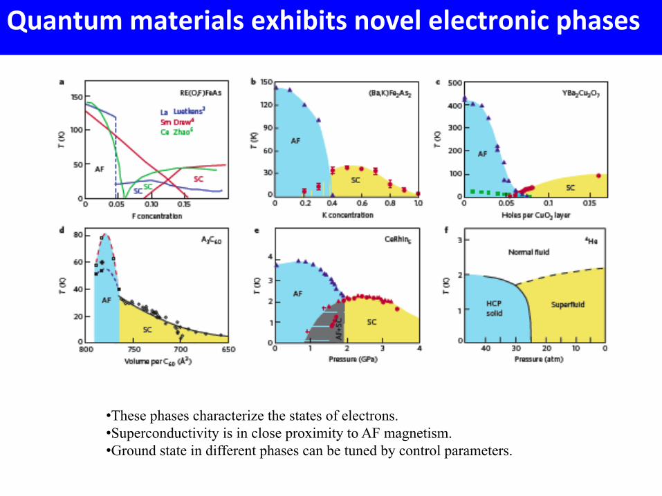
Quantum  materials  exhibits  novel  electronic  phases  

• These phases characterize the states of electrons. • Superconductivity is in close proximity to AF magnetism. • Ground state in different phases can be tuned by control parameters.

•  Several brands

•  Several competing interactions (kinetic energy, Coulomb energy, electron-lattice coupling)

•  Rich selection of competing orders and transitions between them. Consequently, immense tunability, especially near the transition.

• Electronic inhomgeneity important consequnce of competion.

Spin?

Charge?

Lattice? Orbital?

e

They  emerge  from  compe9ng  interac9ons!  

H. C. Manoharan et al., Nature 403, 512 (2000)

dI/dV maps out eigenmodes!

Quantum  mirages  formed  by  coherent  project  of  electronic  structure  

Stipe, Rezaei & Ho, Science 280, 1732 (1998)

C2H2 C2D2

C2H2: acetylene C2D2: deuterated acetylene

d2I/dV2 maps out the vibration mode!

IETS-­‐STM  observa9on  of  local  inelas9c  scaBering  model  

Experimental evidence for electronic inhomogeneity

in cuprates

S. H. Pan et al., Nature 413, 282 (2001)

1.  Spectra gap varies dramatically on the length scale of 50 Angstrom.

2.  “Coherence peak” positions are symmetric about zero bias.

3.  Coherent peak intensity is suppressed in the wide gap regions.

4.  Low energy part of the tunneling spectra are extremely homogeneous.

McElroy et al., Science 309, 1048 (‘05)

1.  Large gap regions are positively correlated with the oxygen dopants.

2.  A charge density variations are significantly weak.

3.  Oxygen dopants are interstitial

Applications of STM to heavy fermion systems

Perfect correlated electron lattice

Kondo hole system

§  Fano interferene, Kondo lattice formation, and ‘hidden order’ transition in URu2Si2 o  Schmidt et al., Nature 465, 570 (2010) o  Aynajian et al., PNAS 107, 10383

(2010) §  Emerging local Kondo screening and

spatial coherence in the heavy-fermion metal YbRh2Si2 o  Ernst et al., Nature 474, 362 (2011)

§  Kondo holes in U1-xThxRu2Si2 o  Hamidian et al., PNAS 108, 18233

(2011)

Evidence of inhomogeneity in CeRh(In1-xCdx)5

§  Puddle size shrinks with increased pressure. Seo et al., Nat. Phys. 10, 120 (2014)

Elastic tunneling

Metal 1 Metal 2

EF1 E1 E2

Insulating barrier

EF2

E1=E2

Inelastic tunneling

E1=E2+w0

Metal 1 Metal 2

EF1 E1

E2

w0

Insulating barrier

EF2

dIdV(r,V )

d 2IdV 2 (r,V )

ρ(r,E)dρdE(r,E)

STM tunneling conductance

Local density of states

Connec9on  between  theory  and  experiment  

Kondo stripe in Anderson-Heisenberg model

Perfect correlated electron lattice

H = − tijc + µδ ij( )

ij ,σ∑ ciσ

† cjσ + Vcf ciσ† fiσ +H.c.⎡⎣ ⎤⎦

i,σ∑

+ ε f − µ( )i,σ∑ fiσ

† fiσ + U fi∑ ni↑

f ni↓f + JH

2Si i Sj −

nif nj

f

4⎛

⎝⎜⎞

⎠⎟ij∑

Slave-boson approach for Ufà∞ fiσ = f iσbi†

fiσ†f iσ + bi

†bi = 1MFA: bi treated as a c-number

Heff = − tij

c + µδ ij( )ij ,σ∑ ciσ

† cjσ + Vcfbiciσ† f iσ +H.c.⎡⎣ ⎤⎦

i,σ∑ − χ ij − ε f + λiσ − µ( )δ ij( )

ij ,σ∑ f iσ

†f iσ

Anderson-Bogoliubov-de Gennes Equations

hijc Δij

Δ ji* hij

f

⎛

⎝⎜⎜

⎞

⎠⎟⎟j

∑ujσn

vjσn

⎛

⎝⎜⎜

⎞

⎠⎟⎟= En

uiσn

viσn

⎛

⎝⎜⎜

⎞

⎠⎟⎟

hijc = −tij

c − µδ ij ,Δij =Vcfbiδ ij

hijf = −χ ij + ε f + λiσ − µ⎡⎣ ⎤⎦δ ij

Numerical details: Supercell technique [JXZ et al., PRB 59, 3353 (1999)] T=0.01, χ=0.1 (input parameter) N×N=24×24

JXZ, Martin, Bishop, PRL 100, 236403 (2008)

Staggered Kondo Phase in the PM regime

bi = b0bi = b0 (−1)

(ix+ iy)

Q=(0,0) Q=(π,π)

(a) (b)

(a) Normal Kondo Phase

(b) Staggered Kondo Phase

c

f

In an infinite-U Anderson-Heisenberg model, SKP is lower in energy than NKP for a uniform RVB OP χ>0 and vice versa.

JXZ, Martin, Bishop, PRL 100, 236403 (2008)

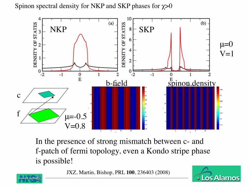
Spinon spectral density for NKP and SKP phases for χ>0

c

f

In the presence of strong mismatch between c- and f-patch of fermi topology, even a Kondo stripe phase is possible!

NKP SKP

b-field spinon density

μ=0 V=1

μ=-0.5 V=0.8

JXZ, Martin, Bishop, PRL 100, 236403 (2008)

H = H0 + Himp

H0 = − tijc + µδ ij( )

ij ,σ∑ ciσ

† cjσ + Vcf ciσ† fiσ +H.c.⎡⎣ ⎤⎦

i,σ∑ + ε f − µ( )

i,σ∑ fiσ

† fiσ + U fi∑ ni↑

f ni↓f

Himp = εcI

σ∑ cIσ

† cIσ + ε fI − ε f( )

σ∑ fIσ

† fIσ + VcfI −Vcf( )cIσ† fIσ + H .c.⎡⎣ ⎤⎦

σ∑ −U fnI↑

f nI↓f

Kondo hole: Level at εfI unoccupied

Kondo Hole Model

Density-matrix Gutzwiller approx.

Heff = H0 + Himp

H 0 = − tijc + µδ ij( )

ij ,σ∑ ciσ

† cjσ + Vcf giσciσ† f iσ +H.c.⎡⎣ ⎤⎦

i,σ∑ + ε f + λiσ − µ( )

i,σ∑ f iσ

†f iσ + U f

i∑ di +Cont

Himp = εcI

σ∑ cIσ

† cIσ + ε fI − ε f( )

σ∑ f Iσ

†f Iσ + Vcf

I −Vcf( )cIσ† f Iσ + H .c.⎡⎣ ⎤⎦σ∑ −U f

λiσ: Lagrange multiplier di: double occupation

giσ (~√qi a): Local renormalization parameter

giσ =niσ

f − di( ) 1− nif + di( )niσ

f 1− niσf( )

⎡

⎣⎢⎢

⎤

⎦⎥⎥

1/2

+di niσ

f − di( )niσ

f 1− niσf( )

⎡

⎣⎢⎢

⎤

⎦⎥⎥

1/2

subject to constraint

λiσ =Vcf∂giσ '∂niσ

fσ '∑ ciσ '

† f iσ ' + c.c.( )−U f =Vcf

∂giσ '∂diσ '

∑ ciσ '† f iσ ' + c.c.( )

aJ.-P. Julien and J. Bouchet, Prog. Theor. Chem. Phys. 15, 509 (2006)

U→∞ :giσ = 1− ni

f

1− niσf

⎡

⎣⎢

⎤

⎦⎥

1/2

Again Anderson-Bogoliubov-de Gennes Equations

hijc Δij

Δ ji* hij

f

⎛

⎝⎜⎜

⎞

⎠⎟⎟j

∑ujσn

vjσn

⎛

⎝⎜⎜

⎞

⎠⎟⎟= En

uiσn

viσn

⎛

⎝⎜⎜

⎞

⎠⎟⎟

hijc = −tij

c − µδ ij + ε Icδ iIδ ij ,

Δij =Vcf giσ 1−δ iI( ) +δ iI⎡⎣ ⎤⎦δ ij

hijf = ε f + λiσ( ) 1−δ iI( ) + ε Ifδ iI − µ⎡⎣ ⎤⎦δ ij

LDOS (Gutzwiller QP):

ρiσc E( ),ρiσc f

E( ),ρiσf E( )( ) = − uiσ

n 2,uiσ

n viσn , viσ

n 2( )n∑ ∂ fFD E − En( )

∂E

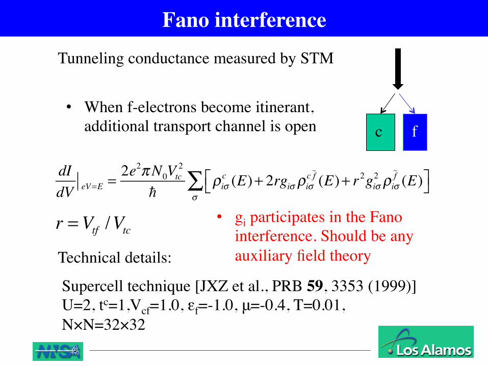
Fano interference

dIdV eV=E =

2e2πN0Vtc2

ρiσc (E)+ 2rgiσ ρiσ

c f (E)+ r2giσ2 ρiσ

f (E)⎡⎣ ⎤⎦σ∑

Tunneling conductance measured by STM

r =Vtf /Vtc

c f •  When f-electrons become itinerant,

additional transport channel is open

Technical details:

Supercell technique [JXZ et al., PRB 59, 3353 (1999)] U=2, tc=1,Vcf=1.0, εf=-1.0, μ=-0.4, T=0.01, N×N=32×32

•  gi participates in the Fano interference. Should be any auxiliary field theory

(a)

−15 0 16 −15

0

16

0.95

0.96

0.97

0.98

0.99

1

(b)

−15 0 16 −15

0

16

0.2

0.4

0.6

0.8

(c)

−15 0 16 −15

0

16

0

0.05

0.1

(d)

−15 0 16 −15

0

16

0.75

0.8

0.85

0.9

0.95

(e)

−15 0 16 −15

0

16

0.2

0.4

0.6

0.8

(f)

−15 0 16 −15

0

16

−0.6

−0.4

−0.2

Solution to the Kondo hole problem

gi λi

di nic

nif ni

c f

JXZ, Julien, Dubi, Balatsky, PRL 108, 186401 (2012)

In the presence of strong mismatch between c- and f-patch of fermi topology, even a Kondo stripe phase is possible!

0

2

4

6

8

10

(a1)

(× 10)

0

0.1

0.2

0.3

0.4(a2)

0

1

2

3

4

(b1)

0

5

10

15

(b2)

−0.25 0.0 0.25 0.5 0.75 −6

−4

−2

0

2

(c1)

E−0.25 0.0 0.25 0.5 0.75

−1.5

−1

−0.5

0

0.5

1

(c2)

E

Gutzwiller QP LDOS

On the Kondo hole site NN to Kondo hole site

ρic(E)

ρif (E)

ρic f (E)

ε If = 1.0, ε I

c = 0.0ε If = 100.0, ε I

c = 0.0ε If = 100.0, ε I

c = −1.0

JXZ, Julien, Dubi, Balatsky,PRL 108, 186401 (2012)

§  Fano interference induces asymmetric dI/dV.

§  Impurity bound states robust against Fano interference.

−0.25 0.0 0.25 0.5 0.75 0

2

4

6

8

10

(a)

(× 10)

E−0.25 0.0 0.25 0.5 0.75

0

0.2

0.4(b)

E

(c)

−15 0 16 −15

0

16

0.05

0.1

0.15

(d)

−15 0 16 −15

0

16

0

2

4

6

8

(e)

−15 0 16 −15

0

16

0.2

0.3

0.4

0.5

dI/dV characteristic and imaging

JXZ, Julien, Dubi, Balatsky, PRL 108, 186401 (2012)

r=0.2

§  Single-particle surface band dispersion in TKI.

§  Continuous tunability of TKI between WTKI and STKI.

§  Number of Dirac cones signifies the STKI and WTKI.

!2

!1.5

!1

!0.5

0

0.5

1

1.5

2

E(k

)

!2

!1.5

!1

!0.5

0

0.5

1

1.5

2

E(k

)

!2

!1.5

!1

!0.5

0

0.5

1

1.5

2

E(k

)

!2

!1.5

!1

!0.5

0

0.5

1

1.5

2

E(k

)

!5

!4

!3

!2

!1

0

1

!̄

E(k

)

!5

!4

!3

!2

!1

0

1

!̄

E(k

)

X̄ X̄ M̄ M̄

(b)

(c) (d)

(e) (f)

(a)

Impurity states on the surface of TKI

Dzero et al, PRL (2010)

Wang, Julien, JXZ, Nature Commun. (submitted)

Hhyb = ciσ† Vcf ,ij ,σα f jα + H .c.⎡⎣ ⎤⎦

ij ,σα∑

Vcf ,ij = dij iσ ,dij = (Vxdijx +Vydij

y +Vzdijz )

§  DOS highly asymmetric w.r.t. Fermi energy for STKI state and dual nature tunable by f-electron energy level

§  DOS is much less asymetric w.r.t. Fermi energy for the WTKI state.

0

0.2

0.4

0.6

0.8

LD

OS

0

0.1

0.2

0.3L

DO

S

!4 !3 !2 !1 0 1 2 3 40

0.2

0.4

0.6

E

LD

OS

Layer 1 (s-band)

Layer 2 (s-band)

Layer 3 (s-band)

Layer 1 (f-band)

Layer 2 (f-band)

Layer 3 (f-band)

(a)

(b)

(c)

Impurity states on the surface of TKI (II)

Wang, Julien, JXZ, Nat. Commun. (submitted)

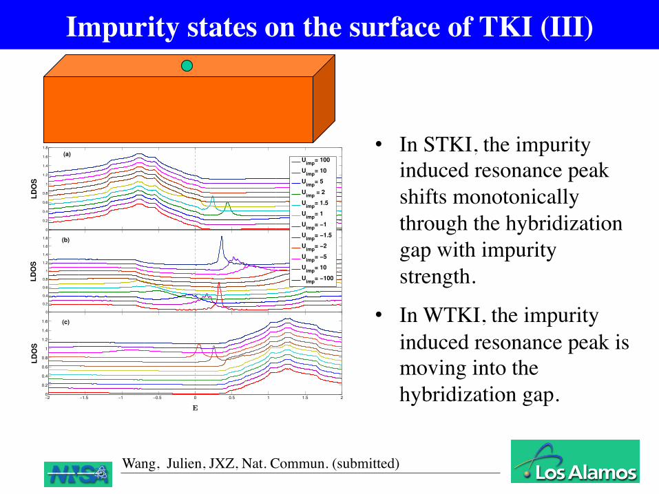
•  In STKI, the impurity induced resonance peak shifts monotonically through the hybridization gap with impurity strength.

•  In WTKI, the impurity induced resonance peak is moving into the hybridization gap.

0

0.2

0.4

0.6

0.8

1

1.2

1.4

1.6

1.8

LD

OS

!2 !1.5 !1 !0.5 0 0.5 1 1.5 20

0.2

0.4

0.6

0.8

1

1.2

1.4

1.6

E

LD

OS

0

0.2

0.4

0.6

0.8

1

1.2

1.4

1.6

1.8

LD

OS

Uimp

= 100

Uimp

= 10

Uimp

= 5

Uimp

= 2

Uimp

= 1.5

Uimp

= 1

Uimp

= !1

Uimp

= !1.5

Uimp

= !2

Uimp

= !5

Uimp

= 10

Uimp

= !100

(b)

(c)

(a)

Wang, Julien, JXZ, Nat. Commun. (submitted)

Impurity states on the surface of TKI (III)

5 10 15 20 25 30

30

25

20

15

10

5

!6

!5

!4

!3

!2

!1

05

1015

2025

3035

0

10

20

30

0

1

2

3

4

5 10 15 20 25 30

30

25

20

15

10

5

!6

!5

!4

!3

!2

!1

05

1015

2025

3035

0

10

20

30

0

0.2

0.4

0.6

0.8

5 10 15 20 25 30

30

25

20

15

10

5

!6

!5

!4

!3

!2

!1

05

1015

2025

3035

0

10

20

30

0

0.5

1

1.5

2

2.5

3

3.5

(a)

(b)

(c)

Impurity states on the surface of TKI (IV)

Wang, Julien, JXZ, Nat. Commun. (submitted)

§  LDOS imaging at resonance energy of STKI and WTKI.

§  Spatial pattern also reveals the nature of TKI.

•  The Gutzwiller and related methods are powerful methods to address electronic inhomogeneity and local electronic structure in heavy fermion.

•  We showcase their applications --- Ø  to predict an alternative phase, Kondo stripe, as a

consequence of Fermi surface mismatch; Ø  to study the local electronic structure around a Kondo-

hole in heavy fermion systems; Ø  to address the nature of impurity induced states in

relation to the topological properties of Kondo insulators.

Summary