JFNK within the semi-implicit scheme in NIMROD

Ben Jamroz, Scott Kruger, Travis Austin Tech-X Corporation jamroz@txcorp.com

NIMROD Meeting: Nov. 6, 2010 Hyatt Regency, Chicago Illinois

http://www.txcorp.com

Outline

•  Previous work: Fully Implicit JFNK –  “Chacon system”

•  JFNK within the semi-implicit scheme •  Analysis of time-stepping Schemes

–  To be applied to fully implicit JFNK

•  Additive Schwarz method •  Conclusion & Future work

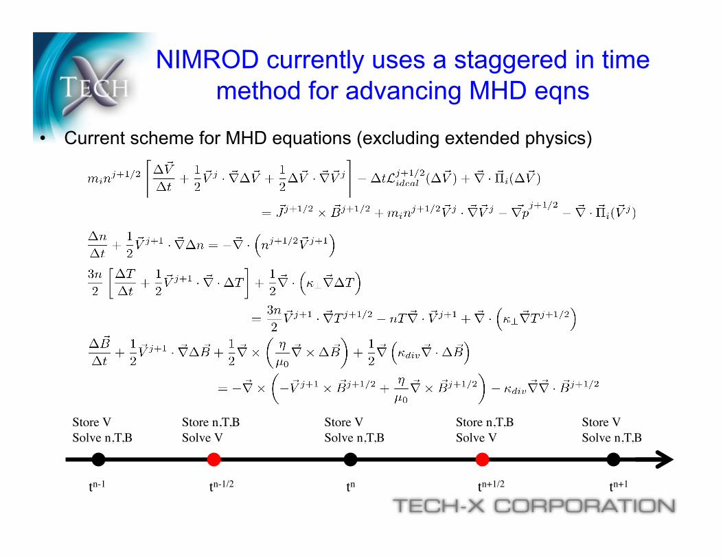
•  Current scheme for MHD equations (excluding extended physics)

NIMROD currently uses a staggered in time method for advancing MHD eqns

tn-1 tn-1/2 tn tn+1/2 tn+1

Store V Solve n,T,B

Store V Solve n,T,B

Store V Solve n,T,B

Store n,T,B Solve V

Store n,T,B Solve V

•  Fully Implicit – Time stepping uses Crank-Nicholson (CN) –  Overcomes time step limitations due to nonlinearities such as

advection, temperature-dependent diffusivities, etc. –  Larger time steps -> Faster time to solve? –  More accurate for a given dt, but

does it matter for problems of interest? •  JFNK - Iterative (Newton type) method to solve nonlinear F(u)=0 •  Action of the Jacobian (in building Krylov subspace) is approximated

–  Don’t need to form the analytical Jacobian •  Preconditioning needed to attain reasonable convergence rates

–  Preconditioner usually a simple approximation to the full Jacobian –  Right preconditioned GMRES –  Physics-based preconditioning (Chacon 2008)

Fully Implicit JFNK potentially has advantages over current scheme

•  Discretized velocity equation

–  Sovinec: Newton method implemented within NIMROD’s infrastructure exploiting the bi-linear nature of the operator.

•  Our approach: –  Include the nonlinear term

–  Precondition GMRES using –  Calculate the action of the Jacobian using finite differencing on

Proof-of-principle case focused just on advective operator

•  N=0 Tearing Mode Instability

•  Convergence in 2-3 GMRES its –  Similar to Sovinec’s method

Velocity Results

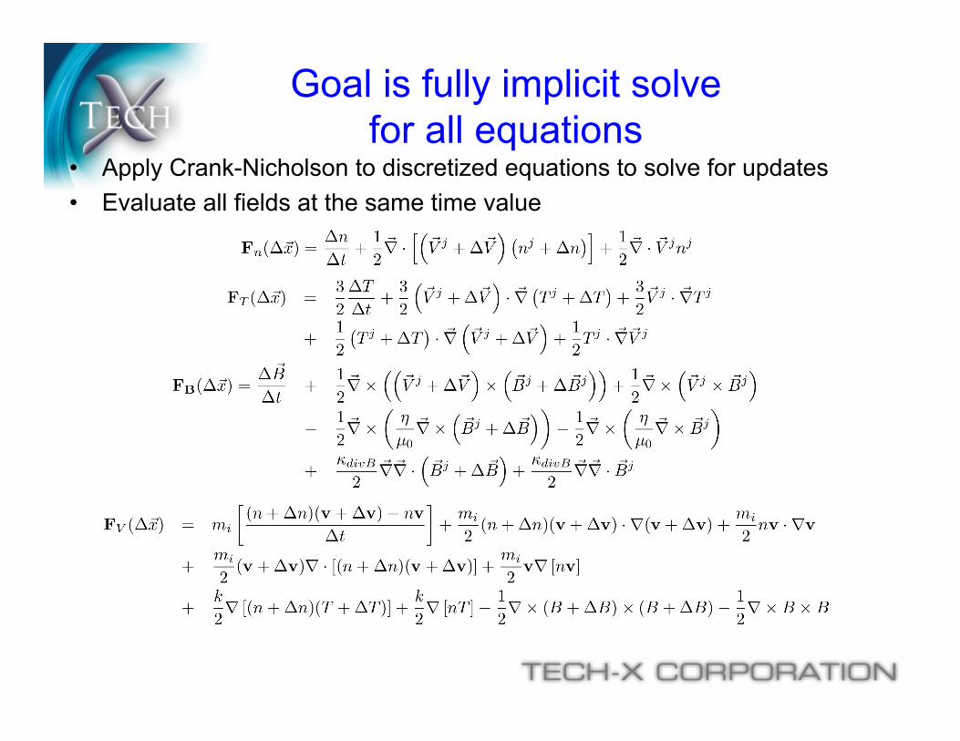
•  Apply Crank-Nicholson to discretized equations to solve for updates •  Evaluate all fields at the same time value

Goal is fully implicit solve for all equations

•  Linearize to compute the Jacobian –  An approximation is used for the preconditioner

•  Define

Symbolic Form for Fully Implicit Solve for MHD system

Extended MHD => M is not diagonal

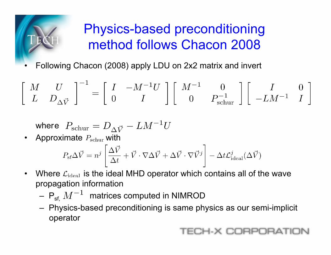
•  Following Chacon (2008) apply LDU on 2x2 matrix and invert

wher e •  Approximate with

•  Where is the ideal MHD operator which contains all of the wave propagation information –  Psf, matrices computed in NIMROD –  Physics-based preconditioning is same physics as our semi-implicit

operator

Physics-based preconditioning method follows Chacon 2008

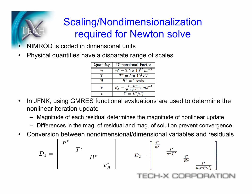
•  NIMROD is coded in dimensional units •  Physical quantities have a disparate range of scales

•  In JFNK, using GMRES functional evaluations are used to determine the nonlinear iteration update –  Magnitude of each residual determines the magnitude of nonlinear update –  Differences in the mag. of residual and mag. of solution prevent convergence

•  Conversion between nondimensional/dimensional variables and residuals

Scaling/Nondimensionalization required for Newton solve

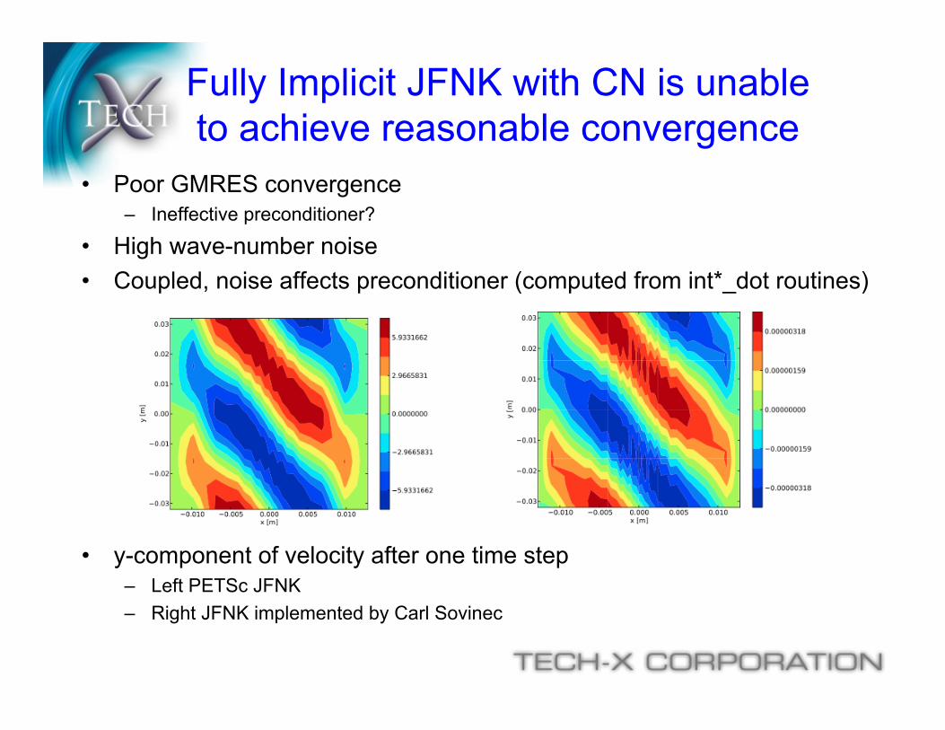
•  Poor GMRES convergence –  Ineffective preconditioner?

•  High wave-number noise •  Coupled, noise affects preconditioner (computed from int*_dot routines)

•  y-component of velocity after one time step –  Left PETSc JFNK –  Right JFNK implemented by Carl Sovinec

Fully Implicit JFNK with CN is unable to achieve reasonable convergence

•  Model Problem: 1D sound wave with damping •  Reinterpret sound speed as Alfven speed •  CN: No damping for large Alfven speed

CN may be responsible for inadequate damping

0.01 0.1 1 10 100 1000 1040.0

0.2

0.4

0.6

0.8

1.0

1.2

!t

Λ#AmplificationFactor

Exact

CN

Semi!Implicit

Parameters taken from slab test case

•  Perhaps noise in solution produced by CN time-stepping –  CN is unable to accurately model diffusion for large dt, large k

•  Implement JFNK within the semi-implicit time stepping scheme –  Velocity solved at t=j*dt, –  n, T, B solved at t=(j+1/2)*dt –  Velocity decoupled, n decoupled – System for B,T only

Side-stepping: JFNK within the semi-implicit scheme

Model dependent nonlinear coupling

•  Thermal conductivity tensor –  Dependent upon magnetic field and temperature –  Braginskii

•  Temperature dependent resistivity

Examples of Nonlinear coupling

•  p_model=aniso1, eta_model = fixed –  Thermal conductivity depends upon B –  B is independent of T

•  p_model=isoropic, eta_model = full –  T independent of B –  Temperature dependent resitivity

•  p_model=aniso_tdep, eta_model = full –  Thermal conductivity depends upon B and T –  Temperature dependent resitivity

•  Currently these couplings are integrated using a predictor-corrector method –  Predict T based on explicit B –  Update B based on predicted value of T –  Correct T based on “implicit” value of B

•  Follow advance_il - Solve for v, n •  Preconditioner for T,B system

–  Assume small differences in –  Full variances of these terms retained in the functional

•  Here D_B and D_T are the matrices for the non-coupled equations –  Already implemented –  Use NIMROD factorization routines

Split JFNK: Implementation Details

Implicit evaluation of nonlinear coefficients is expensive

•  Function evaluations are costly

–  Need to update based on Krylov update –  Vector transfers

•  NIMROD structures Flat (PETSc) vectors

Less iterations, more work…

•  Test case ornl after 1000 time steps –  Ohms=‘hall’ –  p_model=‘aniso_tdep’ –  eta_model=‘eta full’

•  Less GMRES iterations –  More work per GMRES it –  Vector B is 3x larger than T –  One iteration: Full system 4x more work than just T

•  Potential benefit: many B and T iterations

Next Step: JFNK with “mixed” finite element formulation

•  Introduce auxiliary variable for heat flux along mag. Field •  Remain within semi-implicit time-stepping scheme

–  System for q,B,T

•  Jacobian

JFNK with “mixed” finite element formulation – preconditioning ideas

•  JFNK retains full nonlinear behavior in functional •  Simplify the Jacobian to attain an reasonable preconditioner

–  Use explicit magnetic field direction

–  As in system for B,T ignore L_TB and L_BT –  Only invert system for q,T –  Dq mass matrix, L_Tq divergence, L_qT gradient

Diffusion: Crank-Nicholson inaccurate for large time-steps

•  Accurate, stable schemes may not integrate diffusion well •  Model problem •  In the large time steps regime dt>>1

–  Also large wave-numbers or diffusion –  CN: Very little damping for large time steps and wave-numbers –  BE, IMEX-SSP2 (L. Pareschi and G. Russo 2002) successful

0.01 0.1 1 10 100 10000.00.20.40.60.81.0

Ν dt

Λ#Amplificationfactor

Exact

IMEX

MCN

BDF2

BE

CN

L-Stability is important for large time steps!

•  “L-Stable”: Asymptotic preserving –  scheme ensures that –  BE, IMEX, BDF2

•  Effective diffusion: –  Modes that should be strongly damped are somewhat damped –  MCN

0.01 0.1 1 10 100 10000.00.20.40.60.81.0

Ν dt

Λ#Amplificationfactor

Exact

IMEX

MCN

BDF2

BE

CN

Crank-Nicholson can’t handle damped advection

•  CN has difficulty accurately capturing physical diffusion in the presence of strong advection

•  Model problem –  Exact Solution

•  For CN, as gets large

0.001 0.01 0.1 1 10 100 10000.0

0.2

0.4

0.6

0.8

1.0

dt

Λ"AmplificationFactor

CN Α"100

CN Α"10

CN Α"2

CN Α".5

CN Α"0

Exact all Α

Novel integration scheme: Cross between semi-implicit and CN

•  Loureiro and Hammett (JCP 2008) •  Model problem

–  Staggers the evaluation of nonlinear terms –  Formulation done in Fourier space - exactly integrate diffusion

•  Needs efficient preconditioner, here nearly exact •  Initially similar to the Semi-Implicit method

•  Converges to Crank-Nicholson

Additive Schwarz method is a scalable preconditioner

•  Additive Schwarz method (ASM) limits communication –  Approximately applies matrix inversion –  Domain decomposition/processor mapping

•  “Overlapping” Block Gauss-Jacobi relaxation –  Iterative

•  Per-process preconditioner application –  No global LU decomp –  Local decomposition

•  PETSc provides routines for ASM –  Matrices already ported to PETSc –  Can be set from command line options

Multi-level ASM required for an effective preconditioner

•  Many iterations of ASM require a lot of communication •  Introduce a coarse level

–  Many iterations on the coarse level •  Coarse level: linear elements •  Less work since fewer points •  Less communication on lower level

–  Use coarse solution as an initial guess

•  Not directly implemented in PETSc –  Define projection to coarse grid –  Define interpolation from coarse grid

•  Independent Solver on coarse grid

–  ASM/Superlu

•  Fully Implicit JFNK using CN wasn’t effective •  JFNK within the semi-implicit scheme works

–  Hall effects –  Thermal conductivity –  Temperature dependent resistivity

•  Time-stepping schemes –  L-Stability

•  Accurate and stable does not mean it correctly models diffusion –  IMEX, LH08

•  Additive Schwarz Method –  Needs to be multi-level to be competitive

Conclusions

•  Return to fully implicit for the full system –  Using different integration scheme

•  Apply JFNK with a “mixed” finite element formulation –  Within semi-implicit scheme –  Determine effective Preconditioner

•  Implement multi-level Additive Schwarz method

To Do/Future Work