jet substructure at the tevatron and lhc: new...
TRANSCRIPT

Jet Substructure at the Tevatron and LHC:
New results, new tools, new benchmarks∗
A Altheimer1, S Arora2, L Asquith3, G Brooijmans1, J
Butterworth4, M Campanelli4, B Chapleau5, A E Cholakian1,6,
J P Chou7, M Dasgupta8, A Davison4, J Dolen9, S D Ellis10, R
Essig11,12,13, J J Fan14, R Field15, A Fregoso8, J Gallicchio6, Y
Gershtein2, A Gomes16, A Haas11, E Halkiadakis2, V Halyo14, S
Hoeche11, A Hook11,17, A Hornig10, P Huang18, E Izaguirre11,17,
M Jankowiak11,17, G Kribs19,20, D Krohn6, A J Larkoski11, A
Lath2, C Lee21, S J Lee22, P Loch23, P Maksimovic24, M
Martinez25, D W Miller11,17, T Plehn26, K Prokofiev27, R
Rahmat28, S Rappoccio24, A Safonov29, G P Salam30,14,31, S
Schumann32, M D Schwartz6, A Schwartzman11, M Seymour8, J
Shao33, P Sinervo34, M Son35, D E Soper20, M Spannowsky36, I
W Stewart21, M Strassler2, E Strauss11, M Takeuchi26, J
Thaler21, S Thomas2, B Tweedie37, R Vasquez Sierra9, C K
Vermilion38,39, M Villaplana40, M Vos40, J Wacker11, D Walker6,
J R Walsh38,41, L-T Wang14, S Wilbur42 and W Zhu14
1 Columbia University, Nevis Laboratory, 136 S Broadway, Irvington, NY 10533, USA2 Rutgers University, Department of Physics and Astronomy, 136 Frelinghuysen
Road, Piscataway, NJ 08854, USA3 Argonne National Laboratory, 9700 S. Cass Avenue Argonne, IL 60439, USA4 Department of Physics and Astronomy, University College London, WC1E 6BT,
UK5 McGill University, High Energy Physics Group, 3600 University Street, Montreal,
Quebec H3A 2T8, Canada6 Department of Physics, Harvard University, Cambridge, MA 02138, USA7 Department of Physics, Brown University, Box 1843, Providence, RI 02912, USA8 School of Physics and Astronomy, University of Manchester, Manchester, M13 9PL,
UK9 University of California, Davis, Davis, CA 95616, USA10 Department of Physics, University of Washington, Box 351560, Seattle, WA 98195,
USA11 SLAC National Accelerator Laboratory, Menlo Park, CA 94025, USA12 C.N. Yang Institute for Theoretical Physics, Stony Brook University, Stony Brook,
NY 11794, USA
∗Report prepared by the participants of the boost 2011 workshop at Princeton University, May
22–26, 2011. L. Asquith ([email protected]), S. Rappoccio ([email protected]), and C. K. Vermilion
([email protected]), editors.
arX
iv:1
201.
0008
v2 [
hep-
ph]
25
May
201
2FERMILAB-PUB-12-897-T
Operated by Fermi Research Alliance, LLC under Contract No. De-AC02-07CH11359 with the United States Department of Energy.

Jet Substructure at the Tevatron and LHC 2
13 School of Natural Sciences, Institute for Advanced Study, Einstein Drive,
Princeton, NJ 08544, USA14 Department of Physics, Princeton University, Princeton, NJ 08544, USA15 Department of Physics, University of Florida, Gainesville, FL 32611, USA16 Laboratorio de Instrumentacao e Fısica Experimental de Partıculas, 1000-149
Lisboa, Portugal17 Department of Physics, Stanford University, 382 Via Pueblo Mall, Stanford, CA
94305, USA18 Department of Physics, University of Wisconsin–Madison, 1150 University Ave,
Madison, WI 53706, USA19 Fermi National Accelerator Laboratory, Batavia, IL, 60510, USA20 Institute of Theoretical Science, University of Oregon, Eugene, OR 97403, USA21 Center for Theoretical Physics, Massachusetts Institute of Technology, Cambridge,
MA 0213922 Department of Physics, KAIST, Daejeon 305-701, Korea23 Department of Physics, University of Arizona, Tucson, AZ 85719, USA24 Department of Physics and Astronomy, Johns Hopkins University, 3400 N. Charles
St., Baltimore, MD 21218, USA25 ICREA and Institut de Fsica d’Altes Energies, UAB Campus Bellaterra, 08193
Barcelona, Spain26 Institute for Theoretical Physics, Uni Heidelberg, Philosophenweg 16, D-69120
Heidelberg, Germany27 Department of Physics, New York University, 4 Washington Pl, New York, NY
10003, USA28 Department of Physics and Astronomy, The University of Mississippi, University,
MS 38677, USA29 Department of Physics and Astronomy, Texas A&M University, 4242 TAMU,
College Station, TX 77843, USA30 Department of Physics, Theory Unit, CERN, CH-1211 Geneva 23, Switzerland31 LPTHE, UPMC Univ. Paris 6 and CNRS UMR 7589, Paris, France32 II. Physikalisches Institut, Universitat Gottingen, 37077 Gottingen, Germany33 Department of Physics, Syracuse University, Syracuse, NY 13244, USA34 Department of Physics, University of Toronto, 60 Saint George Street, Toronto,
M5S 1A7, Ontario, Canada35 Department of Physics, Yale University, New Haven, CT 06511, USA36 IPPP, Department of Physics, Durham University, UK37 Physics Department, Boston University, Boston, MA 02215, USA38 Ernest Orlando Lawrence Berkeley National Laboratory, University of California,
Berkeley, CA 9472039 Department of Physics & Astronomy, University of Louisville, Louisville, KY
40292, USA40 Instituto de Fısica Corpuscular, IFIC/CSIC-UVEG, PO Box 22085, 46071
Valencia, Spain41 Center for Theoretical Physics, University of California, Berkeley, CA 94720, USA42 Department of Physics, University of Chicago, 5720 S Ellis Ave, Chicago, IL
60637, USA

Jet Substructure at the Tevatron and LHC 3
Abstract. In this report we review recent theoretical progress and the latest
experimental results in jet substructure from the Tevatron and the LHC. We review the
status of and outlook for calculation and simulation tools for studying jet substructure.
Following up on the report of the Boost 2010 workshop, we present a new set of
benchmark comparisons of substructure techniques, focusing on the set of variables
and grooming methods that are collectively known as “top taggers”. To facilitate
further exploration, we have attempted to collect, harmonise, and publish software
implementations of these techniques.
1. Introduction
At the time of the first boost meeting, at SLAC in July 2009, several groups had
begun to argue that jet substructure — the internal characteristics of hadronic jets
— could be useful in identifying the decays of heavy particles at the Large Hadron
Collider. By the following year, a trickle had become a flood. Some techniques had
received detailed attention from experimental groups, and the increasing quantity of
data available meant that background studies were beginning to be possible. Another
year has passed, and the stream of theoretical advances shows no signs of abating. Many
new substructure measurements and techniques have been proposed, and significant
progress has been made in developing the theoretical tools to calculate distributions in
substructure observables. Meanwhile, sufficient data now exist to study the boosted
hadronic decays of heavy Standard Model particles such as the W boson and top quark.
This report, an outgrowth of the boost 2011 workshop held at Princeton University
in May 2011, aims to summarise recent theoretical and experimental progress, outline
goals for the near future, and provide benchmark comparisons and tools to help achieve
these goals.
In Section 2, we review recent substructure results at the Tevatron and LHC. In
Section 3, we survey new proposals for substructure techniques. In Section 4, we describe
the new software tools for studying jet substructure in FastJet 3. In Section 5, we
extend the benchmark top-tagging comparisons found in last year’s report [1] with new
methods, new Monte Carlo samples, and detector simulation. The samples, as well as
software to implement the techniques compared and our detector model, are publicly
available, either as part of the FastJet 3.0.0 package or as FastJet-based tools. Finally,
in Section 6, we survey the status of substructure predictions and discuss goals for new
calculations and measurements in the coming year.
2. New results from the Tevatron and LHC
Several recent experimental results from the Fermilab Tevatron were presented at the
boost 2011 workshop, exploring different aspects of boosted physics. These could be
categorised into two broad classes: studies that elucidate the behaviour of Standard
Model physics processes when subjected to various degrees of boost, and searches for

Jet Substructure at the Tevatron and LHC 4
new physics using boosted object signatures. All the analyses were performed on samples
of√s = 1.96 TeV proton-antiproton collisions produced over the last eight years at the
Tevatron. Results from the Tevatron’s two detectors are presented here in Section 2.1
for CDF and Section 2.2 for D0.
The LHC started colliding protons at a center of mass energy√s =7 TeV on March
30, 2010. Just over 18 months and 5 fb−1 later, the ATLAS and CMS experiments have
collected sufficient data to have a realistic chance of using substructure techniques to
uncover massive boosted particles such as W/Z bosons, top quarks, and whatever else
may lie in wait. The experimental results presented in these proceedings focus on the
results made public prior to the boost workshop in May 2011. For both ATLAS and
CMS this means two analyses: a paper from each on jet shapes [2], [3] and a conference
note on jet substructure [4], [5].
The most important and interesting results of these studies are summarised in
Section 2.3 for ATLAS and Section 2.4 for CMS. Sensitivities to pile-up and detector
effects, seen by the experimental community as the most pressing issues in jet and jet
substructure studies, feature prominently.
All of these experiments must in varying degrees grapple with the presence of
multiple simultaneous proton-(anti-)proton interactions, or pile-up, within every bunch
crossing. These additional collisions are uncorrelated with the hard-scattering process
that triggers the event and create a background of soft diffuse radiation that offsets the
energy measurement of jets and impacts jet shape and substructure measurements. It
is essential that measurements of jet substructure be able to disentangle or correct for
the influence of pile-up.
Observables designed to be sensitive to the internal structure of jets are expected
to also be sensitive to pile-up [1]. Large-radius jets, such as those used in the
measurements of jet substructure, are naturally more susceptible to pile-up due to their
larger catchment area [6]; the invariant mass of these large jets is particularly affected
[7]. Techniques for correcting for these effects — as in the CDF analyses — or mitigating
their impact — such as the splitting and filtering procedure pioneered in ATLAS — are
essential in producing precision measurements for several of the analyses presented by
the Tevatron and LHC experiments. A more thorough review of these issues at ATLAS
can be found in [8].
2.1. Results from CDF
2.1.1. Pile-up at CDF In the context of measurements of the mass, angularity and
planar flow of high-pT jets [9], a new method of correcting the jet mass for pile-up was
developed. The use of a complementary cone at right angles to the jet in azimuthal angle
φ and at approximately the same pseudorapidity allows the energy density from both
underlying event (UE) and multiple interactions (MI) to be measured. The underlying
event refers to the interactions and hadronisation of partons in the colliding protons
other than the partons in the hard process. Multiple interactions refer to both “in-time”

Jet Substructure at the Tevatron and LHC 5
(a) Mass shift. (b) Planar flow shift. (c) Angularity shift.
Figure 1. The correction to the jet mass (a) from additional energy deposition
due to MI+UE (Nvtx > 1 events) compared with the jet mass corrections for
UE alone (Nvtx = 1 events) for jets with a cone size of R = 0.7. The estimated
shift from the combination of UE and MI in planar flow (b) and angularity (c)
as measured in data. The average number of collisions per bunch crossing is ∼3 for this data sample.
and “out-of-time” pile-up: the former describing multiple proton-proton collisions in a
single bunch crossing, the latter describing the delayed instrumental effects of previous
crossings. The incoherent contributions to the shift in jet mass from MI were isolated
from the partially coherent contributions due to UE by examining the mass shift as a
function of the number of good vertices in the event. The average shift in the jet mass
when adding the towers from the complementary cone into the jet are shown in Figure
1 along with the MI+UE corrections measured for angularity and planar flow. The high
mass selections made as part of the angularity and planar flow measurements resulted in
too few events to separate the UE (single-vertex) and MI (single- and multiple-vertex)
components.
2.1.2. New physics searches in multijet events at CDF The results of a search for pair
production of a supersymmetric particle that decays strongly and violates R-parity were
described in [10]. The final state of interest was at least six quarks, most observed as
separate jets, and no missing transverse energy in the event. The challenge for this
search was to reduce the large backgrounds from QCD multijet production, which was
done by placing specific kinematic requirements on three-jet triplets in the final state.
The analysis sought events in a CDF sample that satisfied a trigger requiring at
least four jets with pT > 15 GeV and the sum of the calorimeter transverse energy
greater than 175 GeV. Events were furthermore required to have at least six jets with
pT > 15 GeV and |η| < 2.5, and the scalar sum of the six highest-energy jets was
required to be greater than 250 GeV. The missing transverse energy, /ET , was required
to be less than 50 GeV in order to reduce contributions from W boson final states and
mis-measured QCD events.
All twenty combinations (or more) of three-jet triplets that could be produced from
jets with pT > 15 GeV were considered and the invariant mass of each combination, Mjjj,

Jet Substructure at the Tevatron and LHC 6
and the sum of the magnitudes of the transverse momenta of the three jets,∑
jjj |pT |,were formed. Monte Carlo studies have shown that requiring∑
jjj
|pT | −Mjjj > ∆ (1)
is an efficient way of separating potential signal combinations (where Mjjj would be
a constant reflecting the mass of the supersymmetric parent) from the QCD and
combinatorial backgrounds. ∆ is a constant optimized for each assumed parent mass.
This is in effect a boosted three-jet final state. The shape of the backgrounds in Mjjj
were estimated by using a five-jet final state, showing that the background is expected
to peak around 100 GeV.
The Mjjj distribution was then fit to a combination of signal and background terms,
where the signal was defined by a pythia Monte Carlo calculation for R-parity violating
(RPV) gluino pair production. Although the acceptance for the gluino final state is quite
low (roughly 5× 10⁻⁵), CDF was able to set significant limits on the RPV gluino cross
section, which were then converted into lower limits on the gluino mass. Lower mass
limits ranging from 144 to 154 GeV at 95% C.L. were set on the gluino mass, depending
on the assumptions about the spectrum of intermediate supersymmetric final states.
What is perhaps as interesting is that CDF observed evidence for a boosted top quark
signature. In the top quark mass region of Mjjj ∼ 175 GeV, CDF observed 11 ± 5 jet
triplets. Although one expects on average only one top quark event in this kinematic
region, the shape of the mass distribution is consistent with what one expects from MC
simulations.
2.1.3. Boosted top quark search at CDF CDF presented updated results on the
measurements of jet mass, angularity and planar flow for jets with pT > 400 GeV
from a sample of 5.95 fb−1 [11]. The measured distributions were compared with
analytical expressions from NLO QCD calculations, as well as pythia 6.1.4 predictions
incorporating full detector simulation. The theory predictions for jet mass were in good
agreement with the data, whereas the angularity and planar flow predictions by pythia
showed disagreement in detail (primarily at low angularity and low planar flow).
CDF used these data to also search for a signal of boosted top quark production.
Candidate events were selected in two channels: the fully hadronic decays where both
top quarks produce massive high-pT jets (the “1+1” channel), and the decays where one
top quark decays semi-leptonically resulting in one massive high-pT jet recoiling against
a second lower-mass jet and significant missing transverse energy (the “SL” final state).
A signal region in the 1+1 mode was defined by requiring both leading jets to have a
mass between 130 and 210 GeV (see Figure 2), while the signal region in the SL mode
requires the leading jet to have 130 < mjet1 < 210 GeV and the event to have missing
transverse energy significance
SMET ≡ /ET/√∑
ET ∈ (4, 10). (2)

Jet Substructure at the Tevatron and LHC 7
(a) pythia tt signal. (b) pythia QCD dijets. (c) CDF Run II data, 6 fb−1.
Figure 2. The mjet2 versus mjet1 distribution for all events with at least one jet
with pT > 400 GeV and η < 0.7, using R = 1.0 Midpoint cones. MI corrections
have been performed and all events are required to have SMET < 4.
This cut rejects primarily QCD dijet events. The remaining QCD backgrounds are
estimated by looking at the event rates in sideband regions of jet mass and SMET . The
analysis observes 31 and 26 candidate events in the 1+1 and SL channels, respectively,
and the backgrounds are estimated to be 14.6± 2.7 and 31.3± 8.1 events, respectively.
The total number of top quark events expected in the two channels is 4.9±2.1 candidates.
Although the data are consistent with a boosted top quark signature, they are not
statistically strong enough to claim observation. Rather, they are used to set an upper
limit of 38 fb on top quarks produced with pT > 400 GeV. The SM expectation for this
cross section is 4.5 fb.
2.1.4. Search for lepton jets at CDF There are several theories beyond the Standard
Model that predict the production of cascades of particles that appear in the final state
as a “lepton jet”. The CDF collaboration reported on a search for such objects using 5.1
fb−1 of√s = 1.96 TeV proton-antiproton collisions at the Tevatron. The search looked
for events with a large number of low-energy leptons produced in association with a W
or Z boson.
Events were selected by performing the standard selection for W or Z boson
candidates, requiring at least one well-identified electron or muon candidate and then
either significant /ET or a second well-identified charged lepton of the same flavour but
opposite charge. A “soft lepton” algorithm was then employed to identify additional
electron or muon candidates down to a transverse momentum of 1 GeV for electrons and
3 GeV for muons. The numbers of events in the zero or one additional lepton bins were
used to scale the expected backgrounds for the signal region defined by two or more
soft lepton candidates. The analysis found that the dominant backgrounds came from
inclusive W+jets production where one or more of the jets were mis-identified, or Drell-
Yan production where the additional leptons were mis-identified jets. Other sources of
background, such was W+c-quark, W+b-quark, tt and di-vector boson production were
also evaluated.

Jet Substructure at the Tevatron and LHC 8
The potential signal was modelled on a benchmark process defined by a neutralino
model with a “hidden” Higgs boson coupled to a dark sector, where the dark sector
particles decay to pairs of charged leptons [12]. The channels with the best signal-to-
background for this model were those with a W or Z boson with at least three additional
muons, either with none or one additional electron; for example, in the channel with a
W+3 additional muons, one expected 1.5±1.2 background events and nine signal events
(only two events were observed). There was no signal observed above background, and
a 95% C.L. upper limit on the production cross section of a W or Z boson produced
in association with a Higgs boson with the expected couplings of 27 fb was set. This
allowed the collaboration to rule out the benchmark model.
This analysis showed the effectiveness of using the lepton jet signatures to search
for evidence of new physics.
2.2. Results from D0
2.2.1. Colour Flow in D0 tt Events The D0 experiment presented recent results
showing how the colour flow that is expected to arise between two jets can be used as a
discriminant to identify W boson hadronic decays in a 5.3 fb−1 sample of tt events [13].
Since the W decay products form a colour singlet, they produce an antenna radiation
pattern, with most soft particles emitted between the two jet directions. The “pull”
of the jets’ radiation toward each other can be used to more effectively identify dijet
systems arising from a specific colour state.
Events were selected by requiring the traditional lepton+jets final state, with a
charged lepton, missing transverse energy and four or more jets. At least two of
the jets had to be tagged as b-quark candidates, resulting in 728 candidate events
with an estimated background rate of 82 ± 9 events in the sample not arising from tt
production. The jet pairs that had an invariant mass within 30 GeV of the W boson
mass were then selected and the shape of the energy depositions studied to look for a
signal consistent with the colour singlet. The minimum relative pull angle for jet pairs
satisfying |mW −mj1j2| < 30 GeV, ∆Rj1,j2 < 2 and |η| < 1 is shown in Figure 3(a). The
expected colour effect in the relative orientations of the jet pulls was observed when
comparing the daughter jets from W boson decays and the b-quark jets, though the
statistical power of the measurement was modest and the kinematics of the pairs of jets
were not identical. A more direct comparison was made by producing Monte Carlo tt
decays with a W boson produced as a colour octet compared with the expected colour
singlet state, and a series of detailed studies were performed to evaluate the systematic
uncertainties on this measurement.
The actual quantity measured was the fraction of singlet W boson decays compared
with the total number, giving
fsinglet = 0.65+0.37−0.38 (stat.)± 0.22 (syst.). (3)
This could be turned into a lower limit on the fraction of singlet decays of fsinglet > 0.277
at 95% C.L. Although this is somewhat higher than the limit that might have been
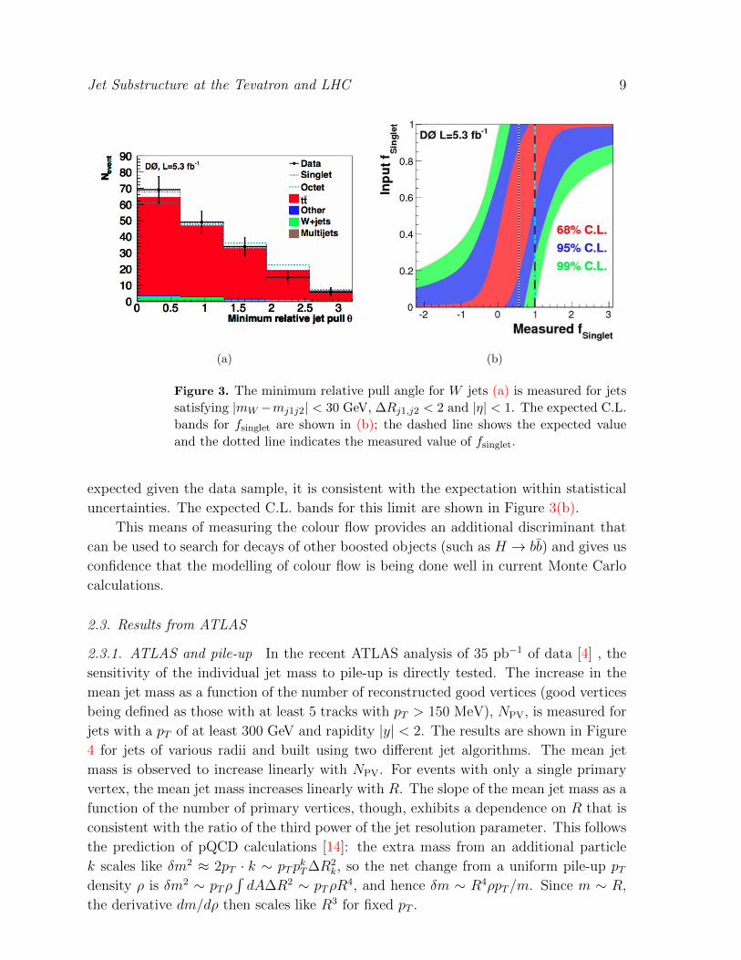
Jet Substructure at the Tevatron and LHC 9
(a) (b)
Figure 3. The minimum relative pull angle for W jets (a) is measured for jets
satisfying |mW −mj1j2| < 30 GeV, ∆Rj1,j2 < 2 and |η| < 1. The expected C.L.
bands for fsinglet are shown in (b); the dashed line shows the expected value
and the dotted line indicates the measured value of fsinglet.
expected given the data sample, it is consistent with the expectation within statistical
uncertainties. The expected C.L. bands for this limit are shown in Figure 3(b).
This means of measuring the colour flow provides an additional discriminant that
can be used to search for decays of other boosted objects (such as H → bb) and gives us
confidence that the modelling of colour flow is being done well in current Monte Carlo
calculations.
2.3. Results from ATLAS
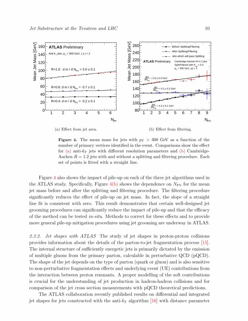
2.3.1. ATLAS and pile-up In the recent ATLAS analysis of 35 pb−1 of data [4] , the
sensitivity of the individual jet mass to pile-up is directly tested. The increase in the
mean jet mass as a function of the number of reconstructed good vertices (good vertices
being defined as those with at least 5 tracks with pT > 150 MeV), NPV, is measured for
jets with a pT of at least 300 GeV and rapidity |y| < 2. The results are shown in Figure
4 for jets of various radii and built using two different jet algorithms. The mean jet
mass is observed to increase linearly with NPV. For events with only a single primary
vertex, the mean jet mass increases linearly with R. The slope of the mean jet mass as a
function of the number of primary vertices, though, exhibits a dependence on R that is
consistent with the ratio of the third power of the jet resolution parameter. This follows
the prediction of pQCD calculations [14]: the extra mass from an additional particle
k scales like δm2 ≈ 2pT · k ∼ pTpkT∆R2
k, so the net change from a uniform pile-up pTdensity ρ is δm2 ∼ pTρ
∫dA∆R2 ∼ pTρR
4, and hence δm ∼ R4ρpT/m. Since m ∼ R,
the derivative dm/dρ then scales like R3 for fixed pT .
Jet Substructure at the Tevatron and LHC 10
pvN
1 2 3 4 5 6
Mea
n Je
t Mas
s [G
eV]
0
20
40
60
80
100
120
140
160 ATLAS Preliminary
> 300 GeV, | y | < 2T
jets, pTAnti k
0.1± = 3.0 PVR=1.0: d m / d N
0.1± = 0.7 PVR=0.6: d m / d N
0.1± = 0.2 PVR=0.4: d m / d N
(a) Effect from jet area.
PVN
1 2 3 4 5 6 7 8 9
Mea
n Je
t Mas
s [G
eV]
80
100
120
140
160
180
200
220
240
260 Before Splitting/Filtering
After Splitting/Filtering
Jets which will pass Splitting
Cambridge-Aachen R=1.2 jets > 0.3
qqSplit/Filtered with R
> 300 GeV, |y| < 2T
p
0.3 GeV± = 2.9 PVdN
dm
0.1 GeV± = 4.2 PVdN
dm
0.2 GeV± = 0.1 PVdN
dm
PreliminaryATLAS
(b) Effect from filtering.
Figure 4. The mean mass for jets with pT > 300 GeV as a function of the
number of primary vertices identified in the event. Comparisons show the effect
for (a) anti-kT jets with different resolution parameters and (b) Cambridge-
Aachen R = 1.2 jets with and without a splitting and filtering procedure. Each
set of points is fitted with a straight line.
Figure 4 also shows the impact of pile-up on each of the three jet algorithms used in
the ATLAS study. Specifically, Figure 4(b) shows the dependence on NPV for the mean
jet mass before and after the splitting and filtering procedure. The filtering procedure
significantly reduces the effect of pile-up on jet mass. In fact, the slope of a straight
line fit is consistent with zero. This result demonstrates that certain well-designed jet
grooming procedures can significantly reduce the impact of pile-up and that the efficacy
of the method can be tested in-situ. Methods to correct for these effects and to provide
more general pile-up mitigation procedures using jet grooming are underway in ATLAS.
2.3.2. Jet shapes with ATLAS The study of jet shapes in proton-proton collisions
provides information about the details of the parton-to-jet fragmentation process [15].
The internal structure of sufficiently energetic jets is primarily dictated by the emission
of multiple gluons from the primary parton, calculable in perturbative QCD (pQCD).
The shape of the jet depends on the type of parton (quark or gluon) and is also sensitive
to non-perturbative fragmentation effects and underlying event (UE) contributions from
the interaction between proton remnants. A proper modelling of the soft contributions
is crucial for the understanding of jet production in hadron-hadron collisions and for
comparison of the jet cross section measurements with pQCD theoretical predictions.
The ATLAS collaboration recently published results on differential and integrated
jet shapes for jets constructed with the anti-kT algorithm [16] with distance parameter

Jet Substructure at the Tevatron and LHC 11
R = 0.6 [2]. The jet shapes were calculated using the constituents associated with the
jets, which were 3D topological calorimeter clusters [17].
The analysis follows similar measurements undertaken by CDF for pp collisions
[18, 19, 20], by ZEUS for e±p [21, 22, 23, 24], and OPAL for e+e− [25, 26] collisions.
The ATLAS analysis uses data corresponding to 3 pb−1 of total integrated
luminosity, collected during 2010. This period of data collection can safely be referred to
as ATLAS’s early days, when pile-up was not the burning issue that it quickly became
in 2011, after about 35 pb−1 had been collected. In 2010 the average number of good
vertices in a single hard scatter was approximately 2. In 2011 data this average is closer
to 10, and increasing with luminosity.
The measurements are carried out for jets with pT > 30 GeV and |y| < 2.8.
The measurements of integrated and differential jet shapes, Ψ (Eq. 5) and ρ (Eq. 4),
are corrected to hadron level and compared to several Monte Carlo predictions. Different
phenomenological models are employed to describe the fragmentation processes and UE
contributions.
The comparisons presented in [2] were complemented with additional results in a
second publication [27] including the predictions from new generators and up-to-date
MC tunes, and are reported in this contribution to the proceedings.
The differential jet shape ρ(r) as a function of the distance r =√
∆y2 + ∆φ2 to
the jet axis is defined as the average fraction of the jet pT that lies inside an annulus of
inner radius r −∆r/2 and outer radius r + ∆r/2 around the jet axis:
ρ(r) =1
∆r
1
N jet
∑jets
pT (r −∆r/2, r + ∆r/2)
pT (0, R), ∆r/2 ≤ r ≤ R−∆r/2, (4)
where pT (r1, r2) denotes the summed pT of the clusters in the annulus between radius
r1 and r2, Njet is the number of jets, and R = 0.6 and ∆r = 0.1 are used.
The points from the differential jet shape at different r values are correlated since,
by definition,∑R
0 ρ(r) ∆r = 1. Alternatively, the integrated jet shape Ψ(r) is defined
as the average fraction of the jet pT that lies inside a cone of radius r concentric with
the jet cone:
Ψ(r) =1
N jet
∑jets
pT (0, r)
pT (0, R), 0 ≤ r ≤ R, (5)
where, by definition, Ψ(r = R) = 1, and the points at different r values are correlated.
A summary of the results presented in [2] are given in Figure 5 for the differential
jet shape in the bin 30 GeV < pT < 40 GeV and in Figure 6 for the integrated jet shape
at r = 0.3 in jets with 30 GeV < pT < 600 GeV.
The measured jets become narrower as the jet transverse momentum and rapidity
increase, although with a rather mild rapidity dependence. The results indicate that
the predicted jet shapes are mainly dictated by the details of the implementation of the
parton showers and the modelling of the underlying event in the Monte Carlo generators.

Jet Substructure at the Tevatron and LHC 12
0.1 0.2 0.3 0.4 0.5
(r)
ρ
-110
1
10 jets, R = 0.6tanti-k
< 40 GeVT
p30 GeV <
| < 2.8y|
ATLAS
DataPYTHIA AMBT1PYTHIA AUET2PYTHIA Perugia2011Pythia 8 4C
r0 0.1 0.2 0.3 0.4 0.5 0.6
Dat
a/M
C
0.81
1.2
(a) pythia tunes.
0.1 0.2 0.3 0.4 0.5
(r)
ρ
-110
1
10 jets, R = 0.6tanti-k
< 40 GeVT
p30 GeV <
| < 2.8y|
ATLAS
DataHW/JIMMY AUET2Hw++ 2.4.2 bugHw++ 2.4.2Hw++ 2.5.1
r0 0.1 0.2 0.3 0.4 0.5 0.6
Dat
a/M
C
0.81
1.2
(b) herwig++ tunes.
0.1 0.2 0.3 0.4 0.5
(r)
ρ
-110
1
10 jets, R = 0.6tanti-k
< 40 GeVT
p30 GeV <
| < 2.8y|
ATLAS
Data 6)→Sherpa 1.2.3 (2 2)→Sherpa 1.2.3 (2 2)→Sherpa 1.3.0 (2
ALPGEN+PYTHIA
r0 0.1 0.2 0.3 0.4 0.5 0.6
Dat
a/M
C
0.81
1.2
(c) sherpa and alpgen.
0.1 0.2 0.3 0.4 0.5
(r)
ρ
-110
1
10 jets, R = 0.6tanti-k
< 40 GeVT
p30 GeV <
| < 2.8y|
ATLAS
DataPOWHEG+PYTHIAPYTHIA AMBT1POWHEG+HERWIGHW/JIMMY AUET1
r0 0.1 0.2 0.3 0.4 0.5 0.6
Dat
a/M
C
0.91
1.1
(d) powheg comparison.
Figure 5. The measured differential jet shape, ρ(r), in inclusive jet production
for jets with |y| < 2.8 and 30 GeV < pT < 40 GeV. Error bars
indicate the statistical and systematic uncertainties added in quadrature. The
measurements are compared to different MC predictions.
The presence of contributions from higher-order pQCD matrix elements in the final state
does not affect the predicted jet shapes significantly.
The pythia, herwig++, and herwig/jimmy Monte Carlo generators, using the
latest tunes to describe minimum bias and underlying-event–related observables in data,
provide a good description of the measured jet shapes, although the latest version of
herwig++ tends to produce jets narrower than the data. As expected, pythia 6
ambt1 tends to produce jets slightly narrower than the data as it underestimates the
UE activity in dijet events [28] and lacks a tuned final-state parton shower from the
initial-state radiation. The effect of the wrong setting in “herwig++ 2.4.2 bug”∗ is
only visible for jets with pT < 40 GeV.
The different sherpa predictions are similar and provide a reasonable description
∗The ATLAS Monte Carlo generation of herwig++ 2.4.2 had the wrong settings for parameters
controlling the multiple-parton interactions.

Jet Substructure at the Tevatron and LHC 13
100 200 300 400 500 600
(r =
0.3
)Ψ
1 -
0.05
0.1
0.15
0.2
0.25
0.3 jets, R = 0.6tanti-k
| < 2.8y|
ATLAS
Data
PYTHIA AMBT1
PYTHIA AUET2
PYTHIA Perugia2011
Pythia 8 4C
(GeV)T
p0 100 200 300 400 500 600
Dat
a/M
C
0.60.8
11.21.4
(a) pythia tunes.
100 200 300 400 500 600
(r =
0.3
)Ψ
1 -
0.05
0.1
0.15
0.2
0.25
0.3 jets, R = 0.6tanti-k
| < 2.8y|
ATLAS
Data
HW/JIMMY AUET2
Hw++ 2.4.2 bug
Hw++ 2.4.2
Hw++ 2.5.1
(GeV)T
p0 100 200 300 400 500 600
Dat
a/M
C
0.60.8
11.21.4
(b) herwig++ tunes.
100 200 300 400 500 600
(r =
0.3
)Ψ
1 -
0.05
0.1
0.15
0.2
0.25
0.3 jets, R = 0.6tanti-k
| < 2.8y|
ATLAS
Data
6)→Sherpa 1.2.3 (2
2)→Sherpa 1.2.3 (2
2)→Sherpa 1.3.0 (2
ALPGEN+PYTHIA
(GeV)T
p0 100 200 300 400 500 600
Dat
a/M
C
0.60.8
11.21.4
(c) sherpa and alpgen.
100 200 300 400 500 600
(r =
0.3
)Ψ
1 -
0.05
0.1
0.15
0.2
0.25
0.3 jets, R = 0.6tanti-k
| < 2.8y|
ATLAS
Data
POWHEG+PYTHIA
PYTHIA AMBT1
POWHEG+HERWIG
HW/JIMMY AUET1
(GeV)T
p0 100 200 300 400 500 600
Dat
a/M
C
0.60.8
11.21.4
(d) powheg comparison.
Figure 6. The measured integrated jet shape, 1 − Ψ(r = 0.3), as a function
of pT for jets with |y| < 2.8 and 30 GeV < pT < 600 GeV. Error bars
indicate the statistical and systematic uncertainties added in quadrature. The
measurements are compared to the different MC predictions considered.
of the data. This indicates that the presence of additional partons from higher-order
matrix elements contributions do not affect the predicted jet shapes, mainly dictated
by the soft radiation in the parton shower. The comparison between sherpa 1.2.3 and
sherpa 1.3.0 shows that the NLL-inspired corrections included in the latter for the
parton shower do not impact significantly the predicted jet shapes. alpgen interfaced
with pythia predicts too-narrow jets and does not describe the data. This was
already the case for alpgen interfaced with herwig/jimmy [2] and requires further
investigation to determine whether the disagreement observed with the data can be
completely attributed to the UE modelling in the MC samples or is also related to the
prescription followed by alpgen in merging the partons from the matrix elements with
the parton showers in the final state.
Finally, powheg interfaced with herwig/jimmy provides a reasonable description
of the data while the interface with pythia predicts too-narrow jets, which is mainly

Jet Substructure at the Tevatron and LHC 14
attributed to the details of the underlying event modelling.
These results confirm the sensitivity jet shape measurements, and their potential
to constrain different Monte Carlo models.
2.3.3. Boosted top quarks with ATLAS First steps have been made this year by ATLAS
in the quest to reconstruct the decay of a boosted top quark in a single jet. The first
publication has been delivered in the context of the search for massive exotic resonances
decaying to tt [29]. This analysis was able to isolate a clean sample of boosted top
quarks.
Figure 7 is an event display showing a candidate boosted top quark event. The
anti-kT jets with R = 0.4 used in the standard ATLAS tt selection are indicated in
red. The result of reclustering the constituents of these jets (topological calorimeter
clusters) with R = 1.0 is shown in green on the same figure. For these events the three
R = 0.4 jets that are combined to form the hadronic top candidate merge into a single
jet when clustered with R = 1.0. These events are thus the first candidates for boosted
top quarks reconstructed as single jets at ATLAS.
Although the statistics with the 2010 dataset were too low to provide a testing
ground for the many substructure techniques and variables we are interested in testing
on such a clean sample of boosted top quarks, the groundwork was laid down to make
the prospects for boosted top analyses on 2011 data very exciting.
2.3.4. Jet substructure with ATLAS One of the most important tasks for the early
ATLAS boosted object analyses was to begin subjecting the various grooming methods
and variables, initially implemented in Monte Carlo, to the tests that come with the
conditions of a real detector. The recent ATLAS analysis on jet mass and substructure
has done just that [4]. The analysis was based on 35 pb−1 of data taken in 2010 and
presented the mass and splitting scale of high pT (> 300 GeV) jets reconstructed with
the anti-kT (R = 1.0) algorithm and with the Cambridge-Aachen (R = 1.2) algorithm at
different stages of grooming. The grooming method employed was a mass-drop filtering
method which looks for hard subjets within the very large parent jet, and discards any
radiation not falling within the subjets designated to the hard splitting. As already
discussed in Section 2.3.1, the behaviour of the mass of large-area jets as a function of
the number of good vertices in an event was studied and the process of filtering away
the soft radiation in such jets was found to effectively remove this dependence. This is
perhaps unsurprising, as the radiation present in an event due to pile-up or underlying
event is expected to be a fairly soft continuum. The analysis discarded all events with
more than one good vertex, focusing on the 28% of the 2010 dataset that is regarded as
being free from pile-up.∗
∗The authors acknowledge that selecting on events with a single primary vertex is a limited
opportunity for ignoring pile-up, as making such a demand in the 2011 data would result in
approximately zero events.

Jet Substructure at the Tevatron and LHC 15
Leptonic top EmissT : ET = 36 GeV, φ = −1.5
electron: pT = 145 GeV, η = 1.1, φ = 2.5
jet: ET = 194 GeV, η = 1.2, φ = 1.7, mj = 16.6 GeV
Hadronic top jet 2, ET = 155 GeV, η = 1.1, φ = −0.7, mj = 22.7 GeV
(R = 0.4 clustering) jet 3, ET = 113 GeV, η = 1.3, φ = −1.7, mj = 14.0 GeV
jet 4, ET = 54 GeV, η = 0.6, φ = −1.7, mj = 8.1 GeV
Hadronic top jet 1, ET = 355.5 GeV, η = 1.3, φ = −1.1
(R = 1.0 clustering)√d12 = 110,
√d23 = 40, mj = 197.1 GeV
Figure 7. Summary table for event 34533931 of run 166658. The leptonic
top candidate is formed by high-pT electron (145 GeV, 10 o’clock), EmissT (1
o’clock), and the b-tagged jet at 12 o’clock. The three anti-kT R = 0.4 jets
between 4 and 6 o’clock are identified as the hadronic top candidate. When
reclustered with R = 1.0 the three jets merge into a single jet with mj = 198
GeV and subjet splitting scales√d12 = 110 and
√d23 = 40 GeV.
The final distributions resulting from the analysis were unfolded to hadron level.
The mass distributions of Cambridge-Aachen jets with R = 1.2 are shown in Figure 8
before and after employing mass-drop filtering with the requirement that the heavier
subjet carry less than µ = 67% of the mass of the parent jet and the splitting between
subjets is fairly symmetric, y2 ≡min(p2T,a, p
2T,b)
m2jet
∆R2ab < ycut2 = 0.09. Figure 9 shows the
mass and splitting scale (√d12 = min(pT,a, pT,b)×∆Rab) of anti-kT jets with R = 1.0.
In all cases the distributions are found to be well modelled by a range of leading-
order parton shower Monte Carlos, to within the systematic uncertainties.

Jet Substructure at the Tevatron and LHC 16
(a) C/A R=1.2 jet mass. (b) Filtered C/A R=1.2 jet mass.
Figure 8. The invariant mass distribution of Cambridge-Aachen R = 1.2
jets (left) and the mass distribution after filtering (right). Both distributions
are unfolded to stable-particle level and compared to pythia, herwig, and
herwig++. The systematic uncertainties are shown by the shaded band.
(a) Anti-kt R=1.0 jet mass. (b) Anti-kt R=1.0 splitting scale.
Figure 9. The invariant mass distribution of anti-kT R = 1.0 jets (left) and the
splitting scale√d12 of the same jets (right). Both distributions are unfolded to
stable-particle level and compared to pythia, herwig, and herwig++. The
systematic uncertainties are shown by the shaded band.

Jet Substructure at the Tevatron and LHC 17
2.4. Results from CMS
2.4.1. CMS and pile-up One advantage of the CMS detector and reconstruction
pipeline is the so-called “particle flow” algorithm for a more holistic approach to jet
reconstruction. Because of this approach, it is possible to remove around 60% of the
pile-up from jets directly as it corresponds to charged tracks which can be associated
to subleading primary vertices. This aids in the reduction of pile-up in jets with
substructure at CMS, and studies show that there is only moderate dependence of
the substructure variables on pile-up for the luminosities considered [5].
The CMS collaboration plans to retain a data-driven approach to measuring mis-
tag rates, ameliorating pile-up issues there. Further studies are ongoing to utilise other
advanced jet reconstruction techniques to further reduce pile-up dependence.
2.4.2. Jet Shapes with CMS Several jet shape measurements have been performed at
CMS similar to those at ATLAS described above in Section 2.3.2. The first is the
examination of the classic jet shapes, and the second is the examination of the jet
charged component structure, both in [3].
Several differences exist between the ATLAS and CMS results. While both
collaborations use the anti-kT jet algorithm, CMS uses different values of the radius
parameter, R. For the inclusive shape measurements, two types of jets were used:
calorimeter-only jets and jets where the calorimeter response was corrected using
associated tracks (“jet-plus-tracks” jets) [30]. To reduce out-of-cone radiation, a large
R of 0.7 was used. The jets were required to have (track-corrected) transverse momenta
greater than 15 GeV. For the charged multiplicity measurement, only the jet-plus-tracks
jets were used, with R = 0.5. The (track-corrected) transverse momenta for the first
two jets were required to be larger than 20 and 10 GeV, respectively.
The distribution of Ψ(r) (Eq. 5) is shown in Figure 10. The Monte Carlo simulation
is doing a very reasonable job at predicting the data, and the agreement improves with
larger transverse momentum.
2.4.3. Boosted top quarks and W bosons with CMS CMS has developed algorithms to
identify the hadronic decays of boosted top quarks and W bosons. The top-tagging
algorithm is based on the Johns Hopkins tagger [31], with small modifications as
described in [32, 1]. The W -tagging algorithm is based on jet pruning [33, 34], adding
a requirement on the mass drop of the subjet splitting, which was motivated by the
BDRS subjet/filter algorithm [35].
The algorithms were characterised as of the boost 2011 conference [5], and
subsequent studies have advanced this characterisation [36]. The strategy for the studies
here is to have data-driven mis-tag predictions which can accurately represent non-top
and non-W backgrounds. Sidebands in the data are selected that have little to no
true top or W contributions, and the tagging rate is derived as a function of the jet
transverse momentum. These per-jet parameterisations are then applied to each jet in

Jet Substructure at the Tevatron and LHC 18
(a) 20 < pT < 30 GeV (b) 40 < pT < 50 GeV
(c) 60 < pT < 70 GeV (d) 80 < pT < 100 GeV
Figure 10. The measured differential jet shape at CMS, ρ(r), in inclusive jet
production for jets with pT > 15 GeV. Error bars indicate the statistical and
systematic uncertainties added in quadrature. The measurements are compared
to MC predictions in different pT bins.
a signal selection, which is used to form a data-driven background estimate. This has
several advantages, primarily that modelling effects are not relevant. Moreover, pile-up
effects are handled directly, because the same data sample is used in the sidebands and
the signal region, so the pile-up contribution is the same.
The efficiency for the tagging algorithms is derived from Monte Carlo, and corrected
for a data-to-Monte-Carlo scale factor using Standard Model tt events in the semi-
leptonic channel in [36]. In that public result, limits are set on the possible cross section
for narrow resonances decaying to tt pairs.
Figure 11 shows the mis-tag rates and efficiencies for the top and W tagging

Jet Substructure at the Tevatron and LHC 19
algorithms from CMS.
(GeV/c)T
Jet p300 400 500 600 700 800 900 1000 1100 1200
To
p M
ista
g R
ate
0
0.02
0.04
0.06
0.08
0.1
0.12 Data
Pythia 6 Tune Z2, Stat Error
Pythia 6 Tune D6T, Stat Error
Pythia 8 Tune 1, Stat Error
Herwig++ Tune 23, Stat Error
Top Tagging AlgorithmCMS Preliminary
= 7 TeVs at -135.97 pb
(a)
(GeV/c)T
Jet p200 400 600 800 10001200 14001600 1800 2000
To
p T
agg
ing
Eff
icie
ncy
0
0.1
0.2
0.3
0.4
0.5
t t →Z`Top TaggingCMS Simulation
= 7 TeVs
(b)
(GeV/c)jet
T p
200 300 400 500 600 700 800 900 1000
W M
ista
g R
ate
0
0.05
0.1
0.15
0.2
0.25
0.3
Data
Pythia 6 Tune Z2, Stat Error
Pythia 6 Tune D6T, Stat Error
Herwig++ Tune 23, Stat Error
= 7TeVs at -134.7 pbCMS PreliminaryJet Pruning Algorithm
(c)
(GeV/c)jet
Tp
200 250 300 350 400 450 500 550 600 650 700
W T
agg
ing
Eff
icie
ncy
0.3
0.35
0.4
0.45
0.5
0.55
0.6
0.65
0.7
0.75
t t→Z'
= 7TeVsat CMS SimulationJet Pruning Algorithm
(d)
Figure 11. Mis-tag rates and efficiencies for the top tagging (top) and W
tagging (bottom) algorithms. The mis-tag rates are measured in a signal-
depleted control sample and compared to pythia and herwig++ predictions.
The efficiencies for tagging top quarks and Ws are estimated from pythia
simulation.
2.4.4. Jet substructure at CMS The study of the performance of jet substructure
techniques in generic QCD samples is critically important to understand these
algorithms, and to derive appropriate sideband regions for data-driven background
estimates at CMS. As such, CMS has performed detailed comparisons of jet substructure
observables in [5].
Jet Substructure at the Tevatron and LHC 20
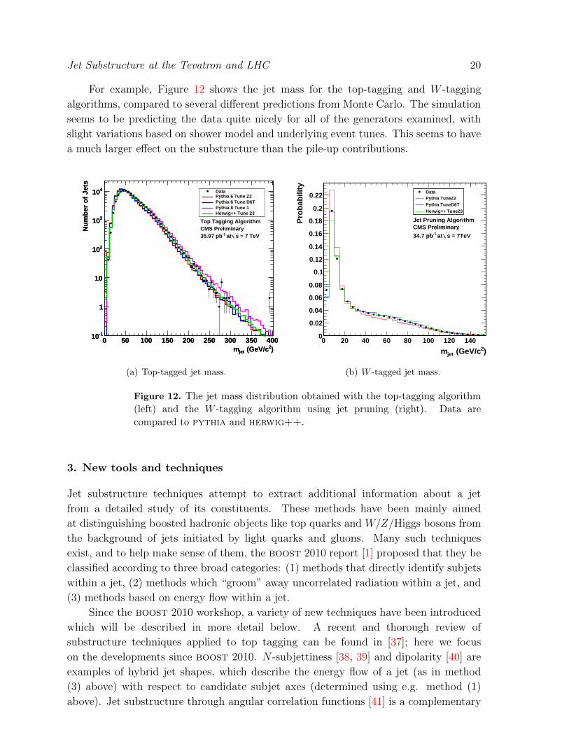
For example, Figure 12 shows the jet mass for the top-tagging and W -tagging
algorithms, compared to several different predictions from Monte Carlo. The simulation
seems to be predicting the data quite nicely for all of the generators examined, with
slight variations based on shower model and underlying event tunes. This seems to have
a much larger effect on the substructure than the pile-up contributions.
)2 (GeV/cjetm0 50 100 150 200 250 300 350 400
Nu
mb
er o
f Je
ts
-110
1
10
210
310
410
)2 (GeV/cjetm0 50 100 150 200 250 300 350 400
Nu
mb
er o
f Je
ts
-110
1
10
210
310
410 DataPythia 6 Tune Z2Pythia 6 Tune D6TPythia 8 Tune 1Herwig++ Tune 23
Top Tagging AlgorithmCMS Preliminary
= 7 TeVs at -135.97 pb
(a) Top-tagged jet mass.
)2 (GeV/cjet m0 20 40 60 80 100 120 140
Pro
bab
ility
0
0.02
0.04
0.06
0.08
0.1
0.12
0.14
0.16
0.18
0.2
0.22DataPythia TuneZ2Pythia TuneD6THerwig++ Tune23
= 7TeVs at -134.7 pbCMS PreliminaryJet Pruning Algorithm
(b) W -tagged jet mass.
Figure 12. The jet mass distribution obtained with the top-tagging algorithm
(left) and the W -tagging algorithm using jet pruning (right). Data are
compared to pythia and herwig++.
3. New tools and techniques
Jet substructure techniques attempt to extract additional information about a jet
from a detailed study of its constituents. These methods have been mainly aimed
at distinguishing boosted hadronic objects like top quarks and W/Z/Higgs bosons from
the background of jets initiated by light quarks and gluons. Many such techniques
exist, and to help make sense of them, the boost 2010 report [1] proposed that they be
classified according to three broad categories: (1) methods that directly identify subjets
within a jet, (2) methods which “groom” away uncorrelated radiation within a jet, and
(3) methods based on energy flow within a jet.
Since the boost 2010 workshop, a variety of new techniques have been introduced
which will be described in more detail below. A recent and thorough review of
substructure techniques applied to top tagging can be found in [37]; here we focus
on the developments since boost 2010. N -subjettiness [38, 39] and dipolarity [40] are
examples of hybrid jet shapes, which describe the energy flow of a jet (as in method
(3) above) with respect to candidate subjet axes (determined using e.g. method (1)
above). Jet substructure through angular correlation functions [41] is a complementary

Jet Substructure at the Tevatron and LHC 21
technique to energy flow observables. The template overlap method [42] and the
shower deconstruction method [43] classify jets with the help of approximations to
hard matrix elements and the parton shower. Beyond the highly boosted regime, the
HEP (Heidelberg-Eugene-Paris) top tagger [44] is appropriate for identifying moderately
boosted top quarks. Meanwhile, substructure techniques have been been used in a
variety of interesting applications, including separating quark jets from gluon jets
[45, 46], tagging jets from initial state radiation [47], and identifying boosted decay
products of new physics [48, 49].
3.1. N-subjettiness
In [38], Thaler and van Tilburg introduced a new jet shape “N -subjettiness” (denoted
τN), designed to identify boosted N -prong hadronic decays. N -subjettiness quantifies
the degree to which jet radiation is aligned along specified subjet axes, such that small
values of τN correspond to N or fewer subjets, while large values of τN indicate more
than N subjets. This jet shape was adapted from the event shape N -jettiness introduced
in [50] to define exclusive jet cross sections, and similar ideas were pursued by Kim in
[39].∗Given candidate subjet directions determined by an external algorithm (such as the
exclusive kT procedure [51, 52]), τN is defined as
τN =
∑k pT,k (min {∆R1,k,∆R2,k, . . . ,∆RN,k})β∑
k pT,k(R0)β, (6)
where the sum runs over the particles in the jet, pT,k is the transverse momentum of
particle k, ∆RA,k is the azimuth-rapidity distance between subjet axis A and particle
k, and R0 is the characteristic jet radius defined such that 0 ≤ τN ≤ 1. The constant β
is an angular weighting exponent closely related to angularities [53], and 1-subjettiness
roughly corresponds to jet angularities [54] with a ≡ 2− β.
To separate boosted hadronic objects from the QCD jet background, one could use
the complete set of τN values (with different values of β) in a multivariate analysis.
However, [38] showed that a simple cut on the ratio τN/τN−1 provides excellent
discrimination power for N -prong hadronic objects. In particular, τ3/τ2 is a successful
boosted top discriminator, and τ2/τ1 can identify boosted W/Z and Higgs bosons, with
the angular weighting exponent β = 1 (corresponding roughly to jet broadening [55])
providing the best discrimination. In subsequent work [56], Thaler and van Tilburg
showed that the initial step of choosing candidate subjet axes is in fact unnecessary. In
particular, the quantity in Eq. 6 can be minimised over the candidate subjet directions
using a variant of the k-means clustering algorithm [57], further improving boosted
object discrimination.
∗[39] focused on boosted Higgs identification, using a Lorentz-invariant version of N -subjettiness
defined in the jet rest frame.

Jet Substructure at the Tevatron and LHC 22
3.2. Dipolarity
A new colour flow observable, “dipolarity”, was introduced by Hook, Jankowiak, and
Wacker to discriminate between different colour configurations of a given pair of subjets
j1 and j2 [40]. Dipolarity is given by a sum in which each constituent of j1+j2 is weighted
by its pT and its squared angular separation ∆R2 from the line segment connecting j1and j2 in the η-φ plane:
D ≡ 1
∆R212
∑i∈J
pT ipTJ
∆R2i . (7)
For subjets j1 and j2 in a colour singlet configuration, the radiation pattern is of
the dipole form with most radiation clustered in the region between the two subjets.
Consequently D is expected to be small for colour singlet configurations and larger for
other colour configurations, in which j1 and j2 are colour connected to other subjets.
By considering the entire radiation pattern of the two subjets at once, dipolarity is
designed to be most effective in the semi-boosted regime, where there can be considerable
overlap between the two subjets. This is in contrast to jet pull [58], which was introduced
with the low boost regime in mind and which can lose discrimination power if there
is substantial overlap. As a first application, dipolarity has been incorporated into the
HEP top tagger [44], where it was shown to improve background rejection by probing the
colour structure of the reconstructed W boson. More work will be needed to determine
whether dipolarity can be applied effectively outside of top tagging.
3.3. Jet substructure without trees
Jankowiak and Larkoski developed a method for identifying substructure within jets via
angular correlations [41], introducing an angular correlation function G(R):
G(R) ≡
∑i6=j
pT ipTj∆R2ijΘ(R−∆Rij)∑
i6=jpT ipTj∆R2
ij
, (8)
where the sum runs over all pairs of jet constituents. The angular correlation function
(ACF) measures the contribution to a jet’s mass from pairs of constituents separated
by an angular scale R or less. A high-pT QCD jet has an ACF that goes approximately
like a power of R, since it is nearly scale-invariant. By contrast, a jet initiated by a
heavy particle decay has one or more intrinsic scales, which results in an ACF with one
or more “cliffs”.∗For a given jet, numerous infrared/collinear-safe observables can be constructed
from the ACF, and these can be used to characterise the jet’s substructure. For example,
one can look at the angular scales at which cliffs are located as well as the corresponding
∗For example, consider a jet with two well-defined narrow subjets. Its ACF will increase steeply
near Rsub, where Rsub is the subjet separation, since pairings of constituents from each subjet begin
to contribute to the sum in Eq. 8 for R & Rsub.

Jet Substructure at the Tevatron and LHC 23
cliff heights. Cliff heights are closely related to mass drops as utilised in BDRS mass-
drop/filtering [35] and can be used to extract mass scales that correspond to hard
substructure in the jet. As a first application of these ideas, Jankowiak and Larkoski
developed a top tagging algorithm whose performance is competitive with others in the
literature. Other applications remain to be explored. Further work on these ideas was
pursued in [59].
3.4. Template overlap
The energy distribution resulting from hard scatterings can be well described by energy
correlation functions in momentum space. In QCD, these naturally describe jet cross
sections in terms of energy flow observables, which are peaked around the states
associated with the hard scattering that subsequently initiate the jets. Therefore, energy
flow observables within the jet should be of particular interest to substructure studies.
In [42], Almeida, Lee, Perez, Sterman, and Sung developed a method based on the
quantitative comparison of the energy flow of observed jets at high-pT with the flow
from selected sets (the templates) of partonic states.
The template overlap procedure can be summarised as follows. Let |j〉 denote the
set of particles or calorimeter towers that make up a jet, identified by some algorithm,
and take |f〉 to represent a set of partonic momenta p1 . . . pn that represent a boosted
decay, found by the same algorithm. The functional measure F(j, f) ≡ 〈f |j〉 quantifies
how well the energy flow |j〉 matches the (templates) |f〉. In practice, [42] found good
results with a simple construction of functional overlap based on a Gaussian in energy
differences within angular regions surrounding the template partons. Any region of
partonic phase space for the boosted decays, {f}, defines a template. Knowledge of the
signal and background can be used to design a custom analysis for each resonance, to
make use of differences in energy flow between signal and background. The template
overlap of an observed jet j is the defined as Ov(j, f [j]) = max {f}F(j, f), the maximum
functional overlap of j to a state f [j] within the template region, where f [j] stands for
the state of maximum overlap, emphasising that the value of the overlap functional
depends not only on the physical state |j〉, but also on the choice for the set of template
functions f .
Template overlaps provide a tool to match unequivocally arbitrary final states j to
partonic partners f [j] at any given order. Once a “peak template” f [j] is found, it can
be used to characterise the energy flow of the state, which gives additional information
on the likelihood that it is signal or background. In addition, template overlaps can
be combined with higher moments of the energy distribution or jet shapes to further
discriminate the event.
3.5. Shower deconstruction
Shower deconstruction, proposed by Soper and Spannowsky, is a method to look for
new physics in a hadronic environment [43]. First, one picks the part of the event

Jet Substructure at the Tevatron and LHC 24
that is likely to be of interest, for instance the part contained in a large-radius jet that
possibly contains the decay products of a boosted heavy particle. This part of the
event is divided into small radius jets called the microjets that are ideally the size of
topoclusters or calorimeter towers. If there are too many microjets to analyse, one can
discard the microjets with the lowest transverse momenta. Shower deconstruction uses
the four-momentum and possibly b-tag information for each microjet.
The aim of shower deconstruction is to calculate a single number χ for each event
such that events with small χ are likely to be background events and events with large χ
are likely to be signal events. The number χ is an approximation to the ratio P (S)/P (B)
of the probability P (S) that a parton shower Monte Carlo that represents the sought
signal process would generate the given event to the probability P (B) that a parton
shower Monte Carlo that represents the background process would generate the event.
The function P (S) is calculated as of a sum, over all possible shower histories for the
signal hypothesis, of weights that are a product of splitting-kernels and Sudakov factors.
P (B) is calculated the same way, but for the background hypothesis.
Although shower deconstruction is not limited to boosted configurations, the
computing time increases strongly with the number of microjets. Boosted configurations
are known to ameliorate combinatoric problems in reconstructing a resonance that
decays hadronically because all decay products can be in one wide angle jet. Thus, [43]
presents a first application of shower deconstruction using the HZ production channel,
where the boosted Higgs decays to a bb pair, first discussed in [35]. The statistical
significance obtained with the shower deconstruction algorithm is found to be larger
than that obtained with the method of [35].
3.6. HEP top tagger
Unlike other taggers, the HEP top tagger, proposed by Plehn, Salam, and Spannowsky, is
not motivated by searches for resonances decaying to two highly relativistic top quarks
[44]. Instead, its first application was the notorious Higgs search channel pp → ttH
with a hadronically decaying H → bb [35]. In the Standard Model, one can expect
several percent of the events to have transverse momenta in the range pT,H & mH and
pT,t & mt, for the leading hadronically decaying top quark. To extract the ttH signal
from the continuum QCD background, [44] required two fat jets, one from a boosted
Higgs and one from a boosted top quark.
Another application of top tagging in a moderately boosted regime is identifying
top partners—like a supersymmetric top squark—decaying to a top quark and an
invisible dark matter agent [60]. Similar to the ttH channel such searches suffer from
combinatoric backgrounds. Using this tagger, one can exploit purely hadronic top decays
and extract the stop pair signal out of backgrounds.
Algorithmically, the HEP top tagger is motivated by the BDRS Higgs tagger. In
particular, it starts with a large, R = 1.5, Cambridge-Aachen jet. This size immediately
translates into a minimum transverse momentum condition of pT,t & 200 GeV. This fat

Jet Substructure at the Tevatron and LHC 25
jet is unclustered using an iterative mass-drop criterion, with a general cutoff at mj > 30
GeV for the subjets. Next, filtering [35] is applied to sets of three hard subjets, using
five constituents, and a combination of three subjets is chosen with jet mass closest to
the top mass. To reconstruct the W mass, notice that for the top decay kinematics, it
is surprisingly likely that more than one of the three mjj combinations lies within 15%
of the W mass. Therefore, the HEP top tagger does not aim to distinguish the b jet
from the two W decay jets, but instead applies a more democratic subjet mass criterion
described in [60]. Finally, a self-consistency condition is applied on the reconstructed
transverse momentum pT,t > 200 GeV.
In a recent application, Plehn, Spannowsky, and Takeuchi studied semi-leptonic
decays of top partners into two top quarks and missing energy [61]. The hadronic top was
reconstructed with the usual tagging algorithm. For the leptonic top, the unmeasured
neutrino three-momentum was reconstructed based on the assumption of a boosted top
decay. Two of the three unknown components can be reconstructed using the top and
W mass constraints. For the third component, one can analyse the top decay in a
specific rest frame and find that one of the neutrino momentum components is strongly
suppressed. This way, one can approximately reconstruct the neutrino momentum and
compare it to the measured two-dimensional missing transverse momentum vector. The
results for supersymmetric top squarks are promising over a wide range of masses with
a similar reach in the hadronic and semi-leptonic channels.
As this report was in preparation, several further extensions of the HEP top tagger
were proposed [62].
3.7. Quark vs. gluon separation
Being able to distinguish light-quark jets from gluon jets on an event-by-event basis
could significantly enhance the reach of many new physics searches at the LHC. The two
prongs of this effort are finding intra-jet observables whose distributions are significantly
different between the flavours, and finding relatively pure samples of quark and gluon
jets to measure these observables in data. Identifying quark and gluon jets was also
studied by ATLAS in the context of reducing jet energy scale uncertainty [63].
In [45], Gallicchio and Schwartz systematically examined many existing and novel
jet substructure observables to find the ones whose distributions, for a given jet η and
pT , are the most powerful single and multi-variable discriminants. It turned out that a
combination of the charged track multiplicity and the pT -weighted linear radial moment
(girth) performed almost as well on particle-level Monte Carlo as discriminants with
more variables. Over 95% of the gluon jets can be filtered out while keeping more than
half of the light-quark jets.
The best single observable was the number of charged particles within the jet (which
were required to have pT > 500 MeV). The discrimination power improved with jet pT ,
and the strength relative to other observables was greatest at high signal efficiency,
where mild cuts were required.

Jet Substructure at the Tevatron and LHC 26
Another good single variable, and part of the best pair, was the linear radial moment
— a measure of the “width” or “girth” of the jet — constructed by adding up the pTdeposits within the jet, weighted by distance from jet axis. It is defined as
g =∑i∈jet
piTpjetT|∆Ri| (9)
where ∆Ri =√
∆y2i + ∆φ2i and where the true boost-invariant rapidity y should be
used when measuring with respect to the (massive) jet axis instead of the geometric
pseudorapidity η. This is a boost-invariant version of jet broadening, to which it reduces
in the limit of massless constituents at small angles to the jet axis.
Finding relatively pure samples was discussed by Gallicchio and Schwartz in [46].
Such samples are necessary because all intra-jet observables have distributions with
significant overlap between quark and gluon jets. Combined distributions of an evenly
mixed sample do not provide verification, independently for quarks and gluons, of the
showering and detector simulation.
Kinematic cuts on multijet and jets+X tree-level samples were optimised to purify
first quarks, then gluons. At the 7 TeV LHC, the pp → γ + 2 jets sample can provide
98% pure quark jets with 200 GeV of transverse momentum and a cross section of 5
pb. To get 10 pb of 200 GeV jets with 90% gluon purity, the pp → 3 jets sample can
be used. These samples could provide a direct evaluation of the tagging technique at
all jet pT ’s, verify and help improve the Monte Carlo generators, and provide a test of
perturbative QCD.
3.8. ISR tagging
In [47], Krohn, Randall, and Wang studied the feasibility of identifying jets from initial
state radiation (ISR) on an event-by-event basis, and considered how these jets can be
used in the interpretation of new physics phenomena. As a proof of principle, they
investigated the pair production of new physics states which each decay into jets and
missing energy, and suggested that ISR can be identified by looking for jets which are
distinguished in either their pT , rapidity, or m/pT ratio. Using these three criteria they
report that they can identify ISR in di-squark (di-gluino) events roughly 40% (15%) of
the time with a mis-tag rate of around 10% (15%).
The most obvious application of the technique is in reducing the combinatoric
difficulties which arise in event reconstruction. However, the production of ISR is
governed by the detailed properties of a hard scattering event, e.g., the flavour of the
initial partons and the scale of the hard interaction, and so ISR can be used to distinguish
between different production mechanisms yielding events with similar visible final states.
In [47], the authors provide an example of this, showing how one can, over many samples,
observe the recoil of a new-physics system against ISR and thus infer the mass scale of
the system even in the presence of significant missing energy.

Jet Substructure at the Tevatron and LHC 27
3.9. Multitagging for New Physics
The application of one or more boosted object taggers can also be used effectively
in searches for the tagged objects within new physics event samples themselves.
This provides the potential to discover the Higgs boson in a way distinct from
Standard Model search strategies, as well as characterising the interactions of the new
physics by understanding the variety of boosted objects that appear in these samples.
Kribs, Martin, Roy, and Spannowsky demonstrated that a slightly modified BDRS
algorithm [35] was highly effective at finding the lightest supersymmetric Higgs boson
in superpartner-enriched event samples, where a boosted Higgs boson appeared in the
cascade from heavy supersymmetric particles decaying to light supersymmetric particles
with a gravitino [48] or neutralino [49] lightest supersymmetric particle. Vector-like
fermionic top partners also provide a rich final state amenable to the simultaneous
application of multiple boosted object taggers. Top-partners decay t′ → (bW, tZ, th)
with roughly (50%, 25%, 25%) branching ratios [64]. Kribs, Martin, and Roy showed that
combining both the HEP top tagger [44] with the BDRS algorithm [35] could identify
both boosted t, boosted h, as well as boosted W/Z (though modified filtering/subjet
techniques). This was shown to be highly effective at identifying top partners with the
Higgs boson in LHC simulations.
4. Jet substructure in FastJet 3
One of the aims of FastJet 3, available since October 2011 from http://fastjet.fr/,
is to facilitate the use and development of jet substructure tools. A novelty relative to
the 2.X series is that jets are now “self-aware”. So whereas previously one would access
a jet’s constituents via its cluster sequence
vector<PseudoJet> constituents = cluster_sequence.constituents(jet);
one may now write
vector<PseudoJet> constituents = jet.constituents();
and similarly for other properties such as parents, subjets and, where relevant, areas.
Aside from being more intuitive to write, this also has the advantage that when dealing
with multiple cluster sequences, one no longer needs to remember which cluster sequence
to use with which jet.
In FastJet 2.X, the only way in which one could create an object with substructure
was by creating a cluster sequence for it. Accordingly a number of tools were written as
plugins, which wasn’t necessarily the most natural way of formulating them. In FastJet
3, an easy way of creating substructure is via the “join” function. Suppose one has
W1, W2 and b subjets obtained from some declustering procedure. Then one may simply
write
PseudoJet W = join(W1,W2);
PseudoJet top = join(W, b);

Jet Substructure at the Tevatron and LHC 28
Transformer ...
TopTaggerBase
Filter
Subtractor
JHTopTagger
XYZTopTagger
Figure 13. Illustration of some of the classes deriving from Transformer in
FastJet 3. Classes shown in dark grey are abstract base classes.
Then, not only will the top’s momentum be sensible, but top.constituents() will return
the concatenation of the constituents of W1, W2 and b. The high-level top substructure
can be accessed with
vector<PseudoJet> top_pieces = top.pieces()
where the vector contains the W and the b. The pieces() function also works on normal
jets from a cluster sequence.
A number of substructure tools are distributed with FastJet 3. They derive from
the Transformer class, and top taggers should derive from TopTaggerBase, as shown in
Figure 13. As an example consider the Filter class, which can be used as follows:
#include "fastjet/tools/Filter.hh"
#include "fastjet/Selector.hh"
double Rfilt = 0.3;
Selector selector_filter = SelectorNHardest(3);
Filter filter(Rfilt, selector_filter);
PseudoJet filtered_jet = filter(jet);
Note the use of the Selector (itself new to FastJet 3), which provides an easy way
of specifying the cuts on the subjets and passing them to the Filter class. Simply
changing the selector leads to trimming [65]
Selector selector_trimmer = SelectorPtFractionMin(0.05);
Filter trimmer(Rfilt, selector_trimmer);
PseudoJet trimmed_jet = trimmer(jet);
Transformed jets often have more internal structure than a normal jet. In the case of
trimmers and filters, for example, one may want to know which subjects did not pass
the selection. For this purpose there is the structure of<TransformerName>() function,
which returns a reference to a transformer-specific class with extra information about
the jet, e.g.,
vector<PseudoJet> rejected_subjets =
filtered_jet.structure_of<Filter>().rejected();

Jet Substructure at the Tevatron and LHC 29
Other substructure tools that are part of FastJet 3 include a Pruner [34], a
MassDropTagger [35], a JHTopTagger [31], and a RestFrameNSubjettinessTagger [39].
Given the rapid evolution of the substructure field, it is not realistic for FastJet to
always distribute a complete and up-to-date set of substructure tools. Accordingly, in
the near future we envisage setting up a FastJet “contrib” area to facilitate dissemination
of third-party tools.
FastJet 3 also contains changes unrelated to substructure. These include a
new interface to pile-up and underlying background estimation, including a new and
very fast grid-based median background estimator. Also of use is a new facility for
attaching arbitrary user information to jets, beyond just the user index of FastJet 2.X.
Illustrations of its usage together with HepMC and Pythia 8 are available on request
from the FastJet authors. More information on these and other developments is to be
found in the FastJet manual, as well as the slides and doxygen documentation on the
FastJet web site [66].
5. Benchmark samples and comparisons
As proposals proliferate for LHC searches with jet substructure, the space of questions
to ask about substructure techniques grows correspondingly larger. Which techniques
work best for which signals? Does the answer depend on the pT of particles in question,
or whether the analysis is a search or a measurement? How do detector limitations
and uncertainties affect each method? How do things change as the amount of pile-up
present increases? If we study these questions with Monte Carlo event generators, do
the answers depend on which generator we choose?
In this section we will address a few of these questions. Beyond the specific results
we give, we hope that the set of samples and tools we use will provide a starting point
for future work. The results here can then be seen as benchmarks for comparison.
Our starting point is the set of comparisons presented in the boost 2010 report
[1]. That analysis compared top taggers exclusively for several reasons. A large number
of substructure techniques are either designed for finding tops or can be used that way;
the two-step decay of a top quark is an interesting example to study; and finding top
jets is immediately useful at the LHC. For the same reasons, as well as limited time
and space, we will take the same approach and focus on distinguishing top jets from
pure QCD background.∗ Extending last year’s results, we will consider new techniques,
more Monte Carlo generators — including matched samples, and the effects of a simple
detector model.
Samples new and old are publicly available at
http://tev4.phys.washington.edu/TeraScale and
http://www.hep.louisville.edu/~verm/TeraScale.
∗A thorough exploration of substructure methods for identifying W jets can be found in [67].

Jet Substructure at the Tevatron and LHC 30
5.1. New samples
This year we expand the set of benchmark samples with events generated by the sherpa
and herwig++ Monte Carlos. The sherpa events allow us to examine the effects of
higher-order matrix elements, which should provide a more accurate description of hard
QCD radiation. The herwig++ events are a useful cross-check of last year’s parton-
shower–level results using a current-generation program.∗
5.1.1. Matched samples with sherpa We consider LHC proton-proton collisions at
a center-of-mass energy of 7 TeV. We have simulated the Standard Model processes
tt+X, W/Z +X and pure QCD jets. All samples were produced with version 1.3.1 of
the sherpa event generator [68, 69]. For the electroweak gauge bosons as well as the top-
quarks we consider fully hadronic decays only. For each process we generated samples
of 100,000 unweighted events for pT slices of 100 GeV between 0 . . . 1.6 TeV, resulting
in an almost flat pT distribution when combining all samples. As slicing parameter we
used the maximum of the Monte Carlo top/anti-top pT , the gauge-boson pT for the
W/Z channels, and the leading-jet pT for pure jet production, where parton-level jets
were reconstructed according to the anti-kT algorithm with R = 1.5. For all processes
the slicing cut is applied at the matrix-element level before parton showering is invoked.
To accurately simulate high-pT events and to account for configurations with more
than one hard parton inside a large jet, we employ sherpa’s matrix-element–parton-
shower matching algorithm [70, 71]. We consider the complete sets of tree-level matrix
elements with up to two (four) additional final-state partons for tt and dijet (W/Z)
production from sherpa’s matrix-element generator comix [72]. The matrix elements of
varying multiplicity are consistently combined to form inclusive samples of fully exclusive
events through subsequent parton shower evolution [73] before being subjected to
hadronization. The renormalization and factorization scales are dynamically determined
on an event-by-event basis according to the matching algorithm [70]. For the parton
separation parameter of the matching procedure we use Qcut = 20 GeV. The default
tune of sherpa 1.3.1 for the hadronization and underlying event model parameters was
used.
5.1.2. herwig++ events For comparison with last year’s herwig events we have
also produced samples using herwig++ 2.5.0. The initial state consists of two
beams of protons at a centre-of-mass energy of 7 TeV. The underlying event has
been simulated using the UE7-2 tune, whose parameters can be found at http://
projects.hepforge.org/~herwig/MB_UE_tunes/input_cards/LHC-UE7-2.in. The
samples have been produced using Standard Model matrix elements for QCD 2 → 2
scattering and tt production. Only fully hadronic final states are considered. For each
process 10,000 events were produced for each pT bin of a width of 100 GeV, from 200
∗We omit other possibilities only for reasons of time and space, and not any stance on the superiority
of particular programs.

Jet Substructure at the Tevatron and LHC 31
GeV to 800 GeV for tt production and from 200 GeV to 1.6 TeV for QCD 2 → 2
scattering. The resulting pT distribution when combining all samples is approximately
flat. The pT cut is applied at the level of the hard process. B hadrons have been set
stable through a lifetime cut of 1 ps, for consistency with the herwig samples used for
boost 2010.∗ All other settings have been left as default.
5.2. New tools
The boost 2010 report compared the Johns Hopkins top tagger [31], its CMS variant
[32], an ATLAS tagger based on kT scales [74], the so-called “Thaler and Wang” tagger
based on a similar kinematic variable zcell [75], and a tagger using pruned jet and
subjet masses [33, 34]. Detailed descriptions of these taggers may be found in the
2010 report [1]. To this list we add a trimming-based tagger [65] as well as the HEP
and N-subjettiness taggers described in Section 3.
The HEP tagger used in this section is a somewhat different implementation than
the one described in Section 3, essentially corresponding to the tagger described in
[44].† Rather than apply the subjet mass criteria of [60] we simply identify the W as
the pair of the three identified subjets with mass closest to mW , and measure its mass
and helicity angle as in the JH and CMS taggers. Both schemes make use of the mass
and decay kinematics of the t→ Wb→ qqb system, so after optimising parameters and
measurement cuts it is not clear how much of an improvement the new symmetric mass
cuts give. We leave this question, just as possible optimisations of the tagging cuts [62],
to detailed joint experimental and theoretical studies.
For the N-subjettiness tagger we find subjet axes via “one-pass minimisation” of kTaxes. That is, three subjets are identified via the exclusive kT algorithm, then a single
iteration of the minimisation procedure described in [56] is applied. The parameter β
is set to 1.0.
5.3. General analysis description
As for the 2010 report, all analyses begin with anti-kT jets with R = 1.0, pT > 200
GeV.‡ For the Hopkins, CMS, HEP, and trimmed taggers, jets are first reclustered
with Cambridge-Aachen, which is also the algorithm used in the pruning stage of the
pruned analysis. For the ATLAS and Thaler and Wang taggers jets are reclustered with
kT before measuring substructure. N-subjettiness is a jet shape, so no reclustering is
necessary.
For each tagger, we identify the set of input parameters to be tuned as well as the set
of output variables to cut on. These are given in Table 1. The Hopkins, CMS, and HEP
∗During final preparation of this report, we discovered that due to an apparent bug in Herwig++
2.5.0, B0 hadrons can still decay through mixing.†Specifically, we use version 1.0 of the HepTopTagger.hh code provided by the tagger authors, and
have defined “passing” as the result of the is maybe top() function instead of is masscut passed().‡It would of course be interesting to see what could be accomplished with smaller or larger R values,
especially larger R at lower pT , but we do not consider this possibility here.

Jet Substructure at the Tevatron and LHC 32
taggers all have a built-in method of identifying the W subjet. For fairness, in the other
taggers we include a W -identifying step: the jet (after grooming for pruning/trimming)
is unclustered to three subjets and the pair with the minimum pairwise mass is merged
to form the W . This mimics the W -finding step in the CMS tagger.
Analysis Input parameters Output variables
ATLAS N/A{m0J ,m
kTW , z
1cut, z
2cut
}CMS {δp, δr} {m0
J ,mW , cos θh}Johns Hopkins {δp, δr} {mJ ,mW , cos θh}HEP
{µ,mmax
subjet
}{mJ ,mW , cos θh}
N-subjettiness N/A {m0J , τ3/τ2}
Pruning {zcut, Rcut} {mJ ,mW}Thaler and Wang N/A
{m0J ,m
kTW , zcell
}Trimming
{Rsub, p
fracT
}{mJ ,mW}
Table 1. Input parameters and output variables for each top tagging analysis.
m0J is the jet mass found by the original algorithm; mJ is after any substructure
modification. For the HEP tagger, µ is the mass drop threshold and mmaxsubjet is
the subjet mass where declustering stops.
The optimal output cuts for any given input variables and signal efficiency are found
using TMVA [76]; input variables are scanned with a Python script and the lowest mis-
tag rate is kept for each bin in signal efficiency. To avoid pathological optimisations
where TMVA finds W jets instead of top jets, we require that the jet mass cut have a
lower bound of at least 120 GeV. The statistical noise from fluctuations in the testing
and training samples is significant, so in each efficiency plot a five-point moving average
is applied.
One might not always want to re-optimise the input parameters of a tagger for
each pT range, signal efficiency, etc. To give a sense of how well each tagger performs
without scanning its parameters, we repeat the efficiency scans with a single set of
input parameters. For each Monte Carlo sample, we take the parameters found at the
35% signal efficiency point, in the 500–600 GeV pT bin, as this common point. These
parameters are given in Table 2.
The analyses are implemented in SpartyJet [77, 78], using tools based on FastJet
[79, 66]. All are available either as internal FastJet tools in version 3.0.0 or as
add-ons available on the FastJet tools site at http://fastjet.fr/tools.html. The
Python scripts used to define the analyses, perform the efficiency scans, and make
the plots, along with instructions, can be found on the BOOST 2011 website, http:
//boost2011.org.

Jet Substructure at the Tevatron and LHC 33
Input parameters
Analysis herwig 6.5 herwig++ sherpa
CMS {δp, δr} = {0.028, 0.13} {0.028, 0.20} {0.056, 0.47}HEP
{µ,mmax
subjet
}= {0.93, 54} {1.0, 46} {0.87, 10}
Johns Hopkins {δp, δr} = {0.083, 0.19} {0.056, 0.23} {0.083, 0.27}Pruning {zcut, Rcut} = {0.056, 0.33} {0.056, 0.33} {0.056, 0.22}Trimming
{pfracT , Rsub
}= {0.050, 0.19} {0.050, 0.28} {0.083, 0.28}
Table 2. Input parameters for each tagger, found by scanning over reasonable
values and taking the lowest mis-tag rate for a 35% signal efficiency, in the
500–600 GeV pT bin. These parameters are then used in all plots where input
parameters are not varied. The ATLAS, N-subjettiness, and Thaler and Wang
taggers are not shown as they do not have input parameters.
5.4. Results
We begin with a simple extension of the 2010 results (Figure 3 in [1]). In Figure 14
we show mis-tag vs. efficiency curves for the expanded set of top taggers, as tested
on last year’s herwig 6.5 samples. We can see that the groomed taggers (pruning
and trimming plus mass cuts), “hybrid” taggers that incorporate grooming as well
as measurement (CMS, HEP, JH), and the N-subjettiness jet shape, outperform the
ATLAS and Thaler and Wang taggers, which use subjet measurements exclusively.
The groomed, hybrid, and jet shape taggers are comparable in performance, with the
groomed and N-subjettiness taggers performing best at low signal efficiency. In the
lower set of plots, where we do not scan over input parameters, N-subjettiness performs
noticeably better over most of the efficiency range.
To complement the herwig 6.5 samples from last year, we have generated
equivalent samples in herwig++ as a cross-check. The results are shown in Figure
15. The results are broadly similar to those for herwig 6.5, but the spread between
different methods is reduced. With or without input optimisation, there is no clear
“winner”.
Both Monte Carlo samples used last year were generated via 2 → 2 processes
interfaced with a parton shower; this year we add matched samples from sherpa to
explore the effects of adding higher-order matrix elements. We expect that these higher-
order effects should lead to a more precise description of the hard, wide-angle radiation
that forms the most challenging background to heavy particle jets.
In Figure 16 we repeat the analyses of Figure 14 on matched samples from
sherpa. The pT cuts are the same. Comparing to Figure 14 we see that the different
multijet modelling predicts substantially worse performance for all taggers, presumably
due to enhanced hard substructure in the background. The relative performance of
different taggers, though, is similar to the unmatched samples. Other than ATLAS
and Thaler and Wang, which continue to be less effective, the taggers are extremely

Jet Substructure at the Tevatron and LHC 34
0.1 0.2 0.3 0.4 0.5 0.6 0.7Signal efficiency
10-3
10-2
10-1
Back
gro
und m
is-t
ag
ATLASCMSHEPJHNSubPrunedTWTrimmed
(a) all pT , optimised
0.1 0.2 0.3 0.4 0.5 0.6 0.7Signal efficiency
10-3
10-2
10-1
Back
gro
und m
is-t
ag
ATLASCMSHEPJHNSubPrunedTWTrimmed
(b) pT 500–600 GeV, optimised
0.1 0.2 0.3 0.4 0.5 0.6 0.7Signal efficiency
10-3
10-2
10-1
Back
gro
und m
is-t
ag
ATLASCMSHEPJHNSubPrunedTWTrimmed
(c) all pT
0.1 0.2 0.3 0.4 0.5 0.6 0.7Signal efficiency
10-3
10-2
10-1
Back
gro
und m
is-t
ag
ATLASCMSHEPJHNSubPrunedTWTrimmed
(d) pT 500–600 GeV
Figure 14. Mis-tag vs. efficiency for several top tagging methods, as tested
on herwig 6.5 tt and dijet samples. For Figures (a) and (b), the input
parameters are optimised for each efficiency point. The input parameters for
the unoptimised scans are taken from the 35% efficiency point in Figure (b).
similar in performance. When we do not scan input parameters, N-subjettiness narrowly
outperforms the hybrid taggers.
The plots thus far represent events with no detector simulation. How do the results
change if we add detector resolution effects? In Figure 17, we repeat the analyses, but
acting on events run through a simple calorimeter simulation provided by Peter Loch,
presented at the boost workshop. This simulation smears energy according to a radial
profile based on performance of the ATLAS detector, then groups energy deposits into
calorimeter cells. Each calorimeter cell is then treated as a massless particle with the
direction and total energy of that cell. The resulting events provide a crude proxy for the
real calorimeter output and give us a way to estimate detector effects on substructure
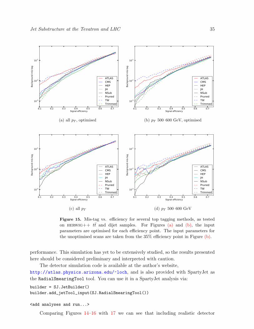
Jet Substructure at the Tevatron and LHC 35
0.1 0.2 0.3 0.4 0.5 0.6 0.7Signal efficiency
10-3
10-2
10-1
Back
gro
und m
is-t
ag
ATLASCMSHEPJHNSubPrunedTWTrimmed
(a) all pT , optimised
0.1 0.2 0.3 0.4 0.5 0.6 0.7Signal efficiency
10-3
10-2
10-1
Back
gro
und m
is-t
ag
ATLASCMSHEPJHNSubPrunedTWTrimmed
(b) pT 500–600 GeV, optimised
0.1 0.2 0.3 0.4 0.5 0.6 0.7Signal efficiency
10-3
10-2
10-1
Back
gro
und m
is-t
ag
ATLASCMSHEPJHNSubPrunedTWTrimmed
(c) all pT
0.1 0.2 0.3 0.4 0.5 0.6 0.7Signal efficiency
10-3
10-2
10-1
Back
gro
und m
is-t
ag
ATLASCMSHEPJHNSubPrunedTWTrimmed
(d) pT 500–600 GeV
Figure 15. Mis-tag vs. efficiency for several top tagging methods, as tested
on herwig++ tt and dijet samples. For Figures (a) and (b), the input
parameters are optimised for each efficiency point. The input parameters for
the unoptimised scans are taken from the 35% efficiency point in Figure (b).
performance. This simulation has yet to be extensively studied, so the results presented
here should be considered preliminary and interpreted with caution.
The detector simulation code is available at the author’s website,
http://atlas.physics.arizona.edu/~loch, and is also provided with SpartyJet as
the RadialSmearingTool tool. You can use it in a SpartyJet analysis via:
builder = SJ.JetBuilder()
builder.add_jetTool_input(SJ.RadialSmearingTool())
<add analyses and run...>
Comparing Figures 14–16 with 17 we can see that including realistic detector

Jet Substructure at the Tevatron and LHC 36
0.1 0.2 0.3 0.4 0.5 0.6 0.7Signal efficiency
10-3
10-2
10-1
Back
gro
und m
is-t
ag
ATLASCMSHEPJHNSubPrunedTWTrimmed
(a) all pT , optimised
0.1 0.2 0.3 0.4 0.5 0.6 0.7Signal efficiency
10-3
10-2
10-1
Back
gro
und m
is-t
ag
ATLASCMSHEPJHNSubPrunedTWTrimmed
(b) pT 500–600 GeV, optimised
0.1 0.2 0.3 0.4 0.5 0.6 0.7Signal efficiency
10-3
10-2
10-1
Back
gro
und m
is-t
ag
ATLASCMSHEPJHNSubPrunedTWTrimmed
(c) all pT
0.1 0.2 0.3 0.4 0.5 0.6 0.7Signal efficiency
10-3
10-2
10-1
Back
gro
und m
is-t
ag
ATLASCMSHEPJHNSubPrunedTWTrimmed
(d) pT 500–600 GeV
Figure 16. Mis-tag vs. efficiency for several top tagging methods, as tested on
sherpa matched tt+ jets and multijet samples. For Figures (a) and (b), the
input parameters are optimised for each efficiency point. The input parameters
for the unoptimised scans are taken from the 35% efficiency point in Figure (b).
resolution generally degrades the best achievable performance and changes how
algorithms compare to each other. Compared to other taggers, N-subjettiness does
worse. For each MC sample the spread between taggers is still small, with the ATLAS
and Thaler and Wang taggers still being outperformed. Considering the right-hand
plots in Figure 17, we can see that in some cases taggers appear to do better after
detector simulation, especially at low signal efficiency. This effect is at least partly due
to statistical noise in the efficiency scans, but warrants further study.
The results we have presented in this report, while certainly not providing the last
word in boosted object tagging, suggest some conclusions. By any metric, methods
that use only subjet kinematic information, like the ATLAS and Thaler and Wang

Jet Substructure at the Tevatron and LHC 37
0.1 0.2 0.3 0.4 0.5 0.6 0.7Signal efficiency
10-3
10-2
10-1
Back
gro
und m
is-t
ag
ATLASCMSHEPJHNSubPrunedTWTrimmed
(a) herwig
0.1 0.2 0.3 0.4 0.5 0.6 0.7Signal efficiency
0.5
0.0
0.5
1.0
1.5
2.0
Back
gro
und m
is-t
ag (
Dete
ctor
- N
o D
ete
ctor)
/(N
o D
ete
ctor)
ATLASCMSHEPJHNSubPrunedTWTrimmed
(b) herwig, fractional difference
0.1 0.2 0.3 0.4 0.5 0.6 0.7Signal efficiency
10-3
10-2
10-1
Back
gro
und m
is-t
ag
ATLASCMSHEPJHNSubPrunedTWTrimmed
(c) herwig++
0.1 0.2 0.3 0.4 0.5 0.6 0.7Signal efficiency
0.5
0.0
0.5
1.0
1.5
2.0B
ack
gro
und m
is-t
ag (
Dete
ctor
- N
o D
ete
ctor)
/(N
o D
ete
ctor)
ATLASCMSHEPJHNSubPrunedTWTrimmed
(d) herwig++, fractional difference
0.1 0.2 0.3 0.4 0.5 0.6 0.7Signal efficiency
10-3
10-2
10-1
Back
gro
und m
is-t
ag
ATLASCMSHEPJHNSubPrunedTWTrimmed
(e) sherpa
0.1 0.2 0.3 0.4 0.5 0.6 0.7Signal efficiency
0.5
0.0
0.5
1.0
1.5
2.0
Back
gro
und m
is-t
ag (
Dete
ctor
- N
o D
ete
ctor)
/(N
o D
ete
ctor)
ATLASCMSHEPJHNSubPrunedTWTrimmed
(f) sherpa, fractional difference
Figure 17. Mis-tag vs. efficiency for several top tagging methods, as tested on
herwig 6.5 and herwig++ tt and dijet samples as well as sherpa matched
tt + jets and multijet samples, all with pT 500–600 GeV. Events have been
run through a simple detector simulation. In the right-hand plots, results after
detector simulation are compared with results before simulation; the y axis
is (εB(detector) − εB(no detector))/εB(no detector). All plots use the input
parameters in Table 2.

Jet Substructure at the Tevatron and LHC 38
taggers, are outperformed by groomed, hybrid, and jet shape taggers. Differences
between the rest of the taggers are largely of similar magnitude to differences between
Monte Carlo samples and before and after detector simulation: more careful study
would be needed to definitively say that some are better than others. In these studies,
the N-subjettiness tagger does particularly well when compared to other taggers with
fixed input parameters, but when optimisation is included performances are extremely
similar. N-subjettiness also appears to be particularly susceptible to degradation due
to detector resolution.
Beyond the limited comparisons given in this section, we hope that the software
tools we have developed to make them will facilitate further study. Such study is clearly
warranted to seriously answer the questions posed at the beginning of this section.
Further phenomenological exploration of the broad space of substructure techniques
will help lead to a more holistic understanding of substructure physics. Monte Carlo
study will complement developments in jet calculations, a subjet to which we now turn.
6. What is calculable and measurable in 2012?
Since the start of the LHC physics program, the ATLAS and CMS experiments have
made substantial progress in measuring jet properties. Interest in using jet properties for
new physics searches has placed a large emphasis on understanding jets more thoroughly
than at previous experiments. The improved resolution of the detectors has made this
possible, and current progress is very promising for the future of jet physics in the age
of the LHC. This has naturally excited the interest of the theory community, whose
continued work on jet physics will confront data in the coming years. This section
is devoted to a summary of theoretical work related to jet substructure, focusing on
observables whose properties can be calculated and measured in the near term.
Two complementary tools are used to understand jet properties: analytic
calculation and Monte Carlo simulation. Analytic calculations give an inclusive picture
of a jet or event, often projecting onto single observables. MC generators offer
totally exclusive events, on which any number of observables can be measured. These
programs can simulate effects that are challenging to integrate into a calculation,
such as the underlying event, pile-up, and hadronisation. State-of-the-art calculations
have perturbative precision that often exceeds MC generators (either in fixed order or
resummed terms), but these calculations are only feasible for a limited set of observables.
Importantly, improvements in analytic calculations help further development and
validation of MC generators. Improvements in calculations will also play a key role
in interpreting jet measurements at the LHC.
Calculations of jet properties typically focus on single jet observables, also known as
jet shapes. These variables are inclusive over the jet constituents, measuring a function
of the final state momenta. By contrast, most jet substructure methods involve more
complicated partitioning of the jet constituents and observables of localised structure in
the jet. While many early studies used subjet information to identify the hadronic decays

Jet Substructure at the Tevatron and LHC 39
of heavy particles, recent studies have explored the efficacy of jet shapes in boosted heavy
object searches (e.g., [38, 41]). Observables derived from the N-subjettiness jet shapes
have been shown to be very competitive in top tagging (see also Section 5). This gives
hope that calculationally simpler observables may be useful in new physics searches.
In this section we will discuss the calculation of jet observables, focusing on jet
mass, which provides an example of a jet observable that can be usefully calculated.
We present aspects of the calculation and discuss improvements that can be made with
future work. We then discuss other observables that are useful for measurement and
point out where calculations may soon be available.
6.1. Jet mass as an example
Jet mass is the simplest and most phenomenologically useful jet shape. An accurate
measurement depends on a good understanding of the jet energy scale and splash-
in contributions (pile-up, the underlying event, and initial state radiation). The
importance of the measurement and the accessibility of the calculation mean that a
comparison between the two can be very useful.
The measurement of a single jet mass is still a complex observable. The calculation
is performed for an exclusive jet multiplicity, meaning there must be a veto on additional
jets. Consider the cross section for dijet events from the anti-kT algorithm, differential
in both jet masses, d2σ/dm1dm2. We must veto on additional jets by placing a pT cut on
candidate jets found by the algorithm. Additionally, the perturbative calculation is only
valid for high-pT jets, meaning a restriction of the phase space for the hard scattering
is required.
There are two main regimes in the jet mass distribution. The small mass regime,
mJ � pTJ , contains large logs of mJ/pTJ . Resummation is required to tame these large
logs and restore accuracy. For larger masses, a fixed order calculation suffices to describe
the distribution. Next-to-leading order is currently state-of-the-art for a wide range of
processes, and can be simulated by Monte Carlo for many processes.
The small jet mass limit is the focus of the most effort in the calculation.
Resummation must be performed in this regime, which requires proving certain
properties of the cross section. In particular, some kind of factorisation must be proven
that relates the all-orders, large-log terms to the fixed order terms.
The additional factorisation required for resummation of jet mass takes two basic
forms, depending on what tools are used. Both perturbative QCD and soft-collinear
effective theory (SCET) can be used to resum the jet mass distribution, and the essential
physics that each uses is the same. However, the language each uses is distinct, and a
comparison of them would be useful. Here we give an outline of factorisation in SCET;
some features of resummation in SCET and QCD are compared in the next subsection.
In the SCET formulation of the cross section, an effective theory framework is used
[80, 81, 82, 83]. Hard modes that produce perturbative emissions of energetic partons
are integrated out of QCD. The remaining soft and collinear modes have momenta

Jet Substructure at the Tevatron and LHC 40
parameterised by a power counting parameter λ � 1. This power counting parameter
is typically determined by the kinematics of the final state; for the jet mass example,
λ = mJ/pTJ . The soft and collinear fields decouple at leading power in the SCET
Lagrangian [83], decoupling the N -jet operators used to describe the energetic jets.
Factorisation also requires showing that the measurement (such as the jet mass with
the anti-kT algorithm and a pT cut on additional jets) factorizes as well. This means the
phase space constraints on soft and collinear modes must separate. This can be shown
formally by providing an operator formulation of the phase space constraints [84, 85],
and can also be seen at a physical level by a power counting analysis of the measurement
in terms of the modes in SCET [86]. This leads to a schematic factorisation theorem of
the form, for N jets:
σ = HN [Ba ×Bb × J1 × · · · × JN ]⊗ SN . (10)
The hard function HN is the matching coefficient onto SCET and arises from the
short-distance interaction that produces the well-separated, energetic partons. The
jet functions Ji and beam functions Ba,b come from the final and initial state collinear
evolution of the hard partons [87]. The soft function SN comes from the global soft
gluon radiation across the event. Each of these functions can be separately calculated
in perturbation theory, and renormalisation group evolution is used to sum the large
logarithms that arise in the cross section. This framework formalises much of the
resummation machinery used in perturbative QCD.
6.1.1. Facets of the calculation We first discuss the perturbative contributions to the
cross section, in particular the resummation. We focus on jets in the anti-kT algorithm,
since jets defined in other algorithms are complicated by the non-trivial role of clustering
between soft gluons. Soft gluon clustering in these algorithms means that the soft phase
space does not factorize into single particle phase space for each soft gluon, affecting
the subleading logarithms in the perturbative series starting at O(α2s ln2) [88, 89]. In
the anti-kT algorithm the phase space for a single soft particle is not affected by the
presence of other soft particles.
The leading logs in the cross section are given by the exponentiation of single soft
gluon emission in QCD, and single-log and running-coupling corrections can be included.
Equivalently in SCET, the leading logs are specified by the cusp anomalous dimensions
of the one-loop jet and soft functions, with the single-log terms coming from the non-
cusp anomalous dimensions. Running-coupling effects arise in renormalisation group
evolution. In the limit of small jet radius (R� 1), the leading logs have the form∫ m
0
dσ
dm∼ σ0 exp
(−αsCF
2πln2 m
pTR2
). (11)
In principle, subleading logarithms can be straightforwardly computed and
resummed. The extension of resummation techniques beyond next-to-leading-log (NLL)
is natural using the SCET framework. However, general jet shapes suffer from non-global

Jet Substructure at the Tevatron and LHC 41
logarithms that contribute at NLL [90]. Nearly every jet measurement made at the LHC
will have non-global observables, and their resummation is more challenging and can
only be performed in the leading-colour approximation [90, 91, 92, 93]. The physics of
the leading non-global logs at fixed order (α2s) has been well understood in QCD, and
their resummation calculated numerically in the large-NC limit. Recent explorations
in SCET have provided additional insights into their structure and origin, providing a
possible new path to renormalisation group-based resummation [94, 95, 96]. Non-global
logs are reduced by soft gluon clustering, and so are reduced for algorithms other than
anti-kT [91, 96].
The small-R approximation is advantageous because a simple picture of non-global
logs emerges. Each jet has its own non-global correction factor, and cross talk between
jets is relegated to a power-suppressed contribution in R. The non-global factor for
a jet was calculated in the large-Nc limit in [90] and used for jet mass in [93]. The
large-Nc approximation will receive corrections from subleading colour terms which will
modify the non-global log contribution at around the ten percent level. Since non-
global logs contribute at NLL and start at O(α2s ln2), subleading terms in colour ought
not to matter phenomenologically, as was the case for deep inelastic scattering event
shapes [97]. Thus in the small-R approximation the cross section is described by a
resummed factor for each jet dressed by a calculated non-global factor, and one can
include jet mass measurements for each jet [93].
Beyond the small-R approximation, one can account for the corrections by including
terms that vanish as powers of R. In QCD, one computes soft gluon emission from all
of the colour dipoles in the event, including the incoming partons. Expanding the result
as a power series in R, one finds that the terms of relative order R2 make a numerical
impact (at around the ten percent level even for R = 0.4), but terms scaling as R4 do
not matter even for R = 1. Similarly, the non-global factor must be corrected beyond
the small-R limit. In SCET, the sum over soft gluon emission from colour dipoles is
given in the soft function, where one expands in
t−1ij ≡tan2R/2
tan2 θij/2, (12)
with θij the angle between jets i and j [98, 54]. The requirement 1/tij � 1 forces the jets
to be well-separated, which is needed to factorize the cross section. When jets become
close together, additional modes in SCET are required to separate the scale dependence
on the small dijet invariant mass [99]. These modes parameterize soft radiation between
the nearby jets, and SCET can be formally extended to SCET+, which includes these
modes.
Therefore, for a wide range of jet mass measurements it should be possible to obtain
a resummed result that accounts for non-global logarithms and goes beyond the small-R
approximation to sufficient accuracy so as to be phenomenologically useful.
A resummed calculation describes the dominant shape of the distribution. However,
many other effects must be taken into account. The shape of the large-mass tail of

Jet Substructure at the Tevatron and LHC 42
the distribution is described well by fixed-order QCD. The resummed and fixed-order
calculations can be combined in a simple way:
dσ
dm=
dσ
dm
∣∣∣∣resum
− dσ
dm
∣∣∣∣FO exp
resum
+dσ
dm
∣∣∣∣FO
. (13)
The resummed and fixed order distributions are added, and the fixed order expansion
of the resummed distribution is subtracted. In the small-mass limit, the two fixed
order functions cancel up to power corrections in m/pT , and the resummed distribution
correctly describes the distribution. In the large-mass tail, the resummed distributions
(all orders and fixed-order expanded) cancel up to the fixed order in αs of the expansion,
so the fixed-order QCD distribution describes the shape up to higher-order corrections.
Hadronisation, pile-up, and underlying event contributions must also be included
in a calculation of the jet mass. These non-perturbative contributions affect the small-
mass regime of the distribution, and are needed for the calculation to be compared to
data. While important, these effects are challenging to include, as no framework exists
to systemically include them and they require a more detailed understanding of the
data.
Basic models have been formulated to quantify contributions from the underlying
event and pile-up [100, 14, 6, 101]. As jet shapes are measured and calculated more
extensively, the comparison between the two is a good testing ground to study these
models and fold them into calculations. In the case of 2-jet event shapes in e+e−
collisions, the correction to the first moment of the event shape from non-perturbative
effects has been shown to be related to a universal, measurable non-perturbative matrix
element for a wide class of event shapes [102, 103]. In the SCET framework, model soft
functions that parameterise non-perturbative effects have also been introduced [104].
Further study is warranted to understand the how non-perturbative effects in a hadron
collider environment can be introduced, and whether similar universality relations that
exist in e+e− collisions apply in the hadron collider case.
6.2. Measurable and calculable observables
A wide array of observables have been defined to study the structure of jets. While
the jet mass is phenomenologically the most important, it is important to prioritise
which other observables should be measured in the near term at the LHC. There
are several key reasons to measure jet substructure. The comparison to precision
QCD calculations is obviously attractive, and understanding QCD backgrounds helps
characterise observables relevant for new physics searches. Additionally, jet substructure
measurements can further understanding of detector effects and improve unfolding
techniques. This can have an impact beyond jet substructure measurements, such as a
reduction in the jet energy scale uncertainty.
There are four general classes of observables used to measure jet substructure and
jetty events:

Jet Substructure at the Tevatron and LHC 43
• Jet mass
• Jet shapes
• Groomed jet observables
• Global event shapes
Although jet mass is a jet shape, it is central enough to jet physics that special
consideration should be given to it as a first measurement. Jet grooming methods
are generic substructure methods that remove isolated soft radiation in jets. Three
grooming methods have been proposed: filtering [35], pruning [33], and trimming [65].
The measurement of properties of groomed jets can provide data about the structure of
the jet that is difficult to capture with simpler observables such as jet shapes. Finally,
global event shapes can be measured without clustering into jets. Several event shapes
are useful in characterising soft physics that can contribute to jet substructure.
Below we discuss each class of observables, identifying key observables in each
category. These are measurements that theorists find informative, and will help in the
study of jet substructure. Many of these observables may be calculated in the near
term, and measurement of them can provide motivation for a detailed comparison.
6.2.1. Jet mass measurements There are several possible channels in which a jet mass
distribution can be measured. These include pure QCD events with inclusive and
exclusive jet cross sections, jets produced in association with electroweak bosons, and
light quark jets produced in association with top quarks. Because the calculation of
a jet mass distribution depends on the precise event topologies studied, to compare
theory and experiment it is important to carefully choose the measurements. Several
key topologies will provide important jet mass measurements. The three we focus on
are γ/W/Z + jet, dijet, and multijet events. In each topology, there are particular jet
mass observables of interest, specialised to the final state.
• γ/W/Z + jet events – These have only a single jet in the final state (assuming
the W or Z decays leptonically) and provide the cleanest jet measurements. This
class of events is an important reference sample for jet energy scale calibration,
and can be used to measure fake rates for certain substructure tagging algorithms.
They are a source of jet + lepton and jet + MET final states, and are a background
to many new physics searches. Theoretically, they can be used as precision tests of
QCD and provide a more calculable environment due to the single jet multiplicity.
The observable of interest is the differential jet mass distribution, dσ/dmJ , in bins
of jet pT . A jet veto must be imposed to obtain an exclusive sample of single jet
events. A hard veto on additional jets, such as pTJ < 0.1 pγT , can be useful for jet
energy scale calibration. The jet mass distribution in this case is of interest because
of the restriction on radiation outside the singe jet. For any value of the jet veto, if
the jet mass distribution is finely binned in pT (several bins instead of one or two),
the impact of various components of the calculation can be compared across pT .

Jet Substructure at the Tevatron and LHC 44
• dijet events – Dijet events with high-pT jets have a large cross section and make
up a significant fraction of the pure QCD events containing high-pT jets at the
LHC. These events are backgrounds to many new physics searches, and their large
cross section means that they must be precisely understood.
Because there are multiple jets in the event, different jet mass measurements can
be made. The doubly differential distribution,
d2σ
dm1dm2
, (14)
with pT1 > pT2, is interesting because correlations between the jet masses can be
studied. This was explored in the CDF analysis of jet mass [105], where the ratio of
event numbers in different bins in the double differential distribution was measured.
Define two single-jet mass bins b1 and b2 (in the CDF study b1 = (30, 50) GeV and
b2 = (130, 210) GeV). These bins define four regions:
A : m1 ∈ b1, m2 ∈ b1 ,B : m1 ∈ b2, m2 ∈ b1 ,C : m1 ∈ b1, m2 ∈ b2 ,D : m1 ∈ b2, m2 ∈ b2 . (15)
(16)
Then define the ratio Rmass to be
Rmass ≡NBNC
NAND
. (17)
If the jet mass distributions were independent, then Rmass = 1. Correlations
between these distribution exist because of soft gluon exchange, although the
expected value of R is not known. This observable is of interest due to the
discrepancy between Monte Carlo simulation and data, and a theory calculation
could help resolve the differences.
In addition to the doubly differential mass distribution, the projection onto a single
mass is theoretically accessible. Common choices are the heavy jet mass and the
sum of jet masses, which have been studied at e+e− colliders. The hardest jet’s
mass is harder to predict theoretically because the relative pT in dijet events is
affected primarily by soft physics.
• multijet events – Events with more than two jets provide a more complex
background. The colour correlations between jets are enhanced as the detector
becomes more crowded, and these events typically have a hierarchy of jet pT ’s.
Multijet events are more important at the LHC due to the increased phase space for
high-pT parton production, and significant attention has been paid to understanding
them better theoretically and experimentally. Multijet events present a theoretical
challenge to describe, but also offer the opportunity to learn about effects such as
colour correlations that figure less prominently in simpler events.

Jet Substructure at the Tevatron and LHC 45
In multijet events, placing a hard pT cut on the leading three jets will give a
multijet event sample that allows one to study the structure of the hardest jet as
the kinematics of the events change. In particular, the jet mass distribution of the
hardest jet can be measured in bins of the ∆R separation to the nearest jet. As jets
become closer together, inter-jet soft radiation can have a large effect on the mass
distribution. This can be predicted theoretically, and the result compared with the
Monte Carlo.
Because the jet mass is sensitive to the environment of the event, it is important to
examine the effect of event-wide characteristics on the mass. As pile-up increases, the
jet mass can serve as a probe of the size of the pile-up and the effectiveness of subtraction
methods (see Section 2.3.1).
The rapidities of the hard jets will affect the jet mass distribution, for a number of
reasons. First, large-rapidity jets imply a large momentum asymmetry between the
initial partons, meaning that one carries a large fraction of the proton momentum
(x ∼ 0.1). Since the quark parton distribution functions dominate in this regime, the
fraction of quark jets will be enhanced relative to central events. Second, the shape of
the parton distribution functions implies there is likely to be more initial state radiation,
since they are less steep in the large x region. Coupled with the fact that the large-
rapidity jets are closer to the beams, it is interesting to see the dependence of jet mass
on the jet rapidity.
Finally, the total transverse momentum in the event, HT , is a measure of the activity
of the event. Soft jets that are vetoed contribute to HT and will affect the jet mass, but
still fit into the same event selection criteria. The contribution of underlying event and
pile-up will similarly affect the jet mass distribution, and HT is a simple proxy for the
size of these observables.
6.2.2. Jet shape measurements Jet shapes measure the radiation pattern within a jet
by calculating a function of the momenta in the jet. The jet mass is a special jet shape,
but there are other important jet shapes whose measurement would be very informative.
We discuss several. Both N -subjettiness and planar flow are calculable, as they take
moments of the momenta in the jet.
• N -subjettiness is a useful variable for jet substructure [38, 56]. N -subjettiness is
defined with respect to a set of subjet axes qi:
τ(β)N =
∑k pT,k (min {∆R1,k,∆R2,k, . . . ,∆RN,k})β∑
k pT,k(R0)β, (18)
where β > 0 is a real parameter, R0 is the radius of the jet, and ∆Ri,k is the angular
separation between particle k and subjet axis qi. The shape τ(β)N probes how “N -
subjet-like” a jet is, and provides an effective veto on additional subjets. Because
adding more axes only lowers the value of τ(β)N , N -subjettiness cannot provide a
veto against fewer subjets.

Jet Substructure at the Tevatron and LHC 46
The case N = 1, β = 1 is also known as girth, broadening, or width; β = 2 is related
to the jet mass for small masses. These are the most common choices for β, and
it would be interesting to compare them. Additionally, other choices of β can be
informative, as they will probe the structure of the jet as a function of the angle to
the 1-subjettiness axis. τ(β)1 is similar to jet angularities, a jet shaped defined for
e+e− events [53, 106, 98, 54]. The distribution in jet angularity τa was calculated
to next-to-leading log accuracy in τa [54], and the theoretical tools exist to extend
this calculation to the distribution of τ(β)1 at the LHC.
2- and 3-subjettiness are also of interest. These can probe jets with multiple subjets,
and the substructure of these jets will more closely resemble a boosted heavy object
decay. (Using τ3/τ2 to identify top jets was studied in Section 5.)
• Planar flow is an interesting shape variable that was proposed to distinguish top
and QCD jets [107, 75]. Planar flow is defined in terms of the eigenvalues of a
2-by-2 matrix, Iw, constructed from the components of momenta perpendicular to
the jet axis:
Iklw =1
mJ
∑i∈J
p⊥ki p⊥liEi
, (19)
where p⊥k is the kth component of p perpendicular to the jet axes (with respect to
a pair of basis axes in the perpendicular plane). From Iw, planar flow is defined
Pf =4 det Iwtr(Iw)2
. (20)
If the radiation in the jet is clustered along a line in the perpendicular plane going
through the jet axis, then Pf will be close to 0. This will be the case for QCD jets
and jets with 2-body kinematics, such as Higgs or W jets. For jets with 3-body (or
more) kinematics, such as the top, Pf will be O(1).
• Subjet and track multiplicities have been shown to be effective discriminators of
quark and gluon jets [45, 46]. Subjets can be found by reclustering the jet with
a small radius, and finer resolution of the subjet size can improve discrimination
between jets from different sources. The study of subjet multiplicity offers the
chance to study the sensitivity to pT or energy cutoffs placed on jet constituents or
subjets. Does the energy resolution for subjets significantly improve with a higher
energy cutoff on jet constituents? Does the multiplicity become sensitive to pile-up
and the underlying event if the cutoff is taken too low? Similarly, the charged track
multiplicity is a useful observable whose power depends on the angular resolution
for track identification as well as the performance over the range of charged particle
momenta in the jet.
6.2.3. Groomed jet measurements Many new physics searches can utilise jet grooming
algorithms. Filtering, pruning, and trimming are jet grooming algorithms that modify
the substructure of the jet to remove contributions from the underlying event and pile-
up [35, 33, 34, 65]. These algorithms can be applied to a wide range of channels, and

Jet Substructure at the Tevatron and LHC 47
comparing the performance of the three algorithms can instructive (cf. Section 6 of
Ref. [1]). Because each algorithm operates on the substructure differently, it is useful
to compare all of them. Experimental studies can quantify the performance of each
algorithm and determine which is best for a given application.
Each grooming algorithm operates on a single jet and produces a groomed jet.
Therefore any observable can be measured on the original jet and the groomed jet. The
distributions before and after grooming are always of interest to understand the effects
of grooming, and grooming algorithms can be used to study a variety of jet properties.
The most interesting observables and objects to study with jet grooming are
• Jet mass.
• Pile-up and the underlying event are a large motivation for jet grooming methods.
The performance with respect to pile-up for some jet grooming algorithms is
currently being studied, and is quantified by studying tracks from secondary
vertices. Quantifying the performance with respect to the underlying event is more
challenging, but measures exist [101].
• If N -subjettiness is measured, then the effect of the grooming algorithms will be
interesting to study. Grooming algorithms are designed to remove isolated soft
radiation that can come from the underlying event or pile-up and contribute to
poor mass resolution in the jet. This radiation will also have a large effect on N -
subjettiness. Studying the N -subjettiness distribution (for N = 1, 2, 3) will give
insight to grooming methods using an observable where it is simple to visualise jets
with multiple energetic subjets.
• Given the good tracking and angular resolution at the LHC, the experiments can
study the performance of grooming methods using only charged tracks.
6.2.4. Global event shapes Finally, event shapes are also of interest. While these are not
direct jet substructure observables, they have a strong connection to jet substructure.
Initial studies of jet substructure were driven by Monte Carlo studies, but more recently
the theoretical foundations of jet substructure have been explored. Event shapes have
traditionally been a testing ground for theoretical tools, and jet shapes are a by-product
of these studies. N -subjettiness was built in analogy to N -jettiness, an event shape
used to veto against additional jets in an event [50, 108, 109]. Like N -subjettiness, N -
jettiness measures how ≤N -jet-like an event is. Measurements of event shapes can be
compared directly to calculations, and the comparison is useful in building theoretical
tools to calculate jet substructure properties. These observables are especially amenable
to calculation, and in fact distributions of these observables have already been calculated
in a variety of applications.
Observables of interest include:
• 0-jettiness, also known as beam thrust, is a measure of total hadronic activity away
from the beams. In events without energetic jets, this can be used to study the
underlying event and assist in tuning the Monte Carlo. In new physics searches

Jet Substructure at the Tevatron and LHC 48
with a veto on any jets (e.g., h→ WW ), the beam thrust distribution can be used
to understand the theory uncertainties on the jet veto.
• 1-jettiness can be similarly implemented on events with a single jet, and can be used
to veto against additional jets for an exclusive 1-jet sample. An ample background
of γ/W/Z+ jet exists in which to study the 1-jettiness distribution.
• A number of event shapes have been proposed for study in dijet type events
in [110] and examined in detail in [111], including observables related to thrust,
broadening and jet rates (Y23). Thrust-like observables show enhanced sensitivity
to the underlying event, possibly allowing for powerful constraints on its properties,
while Y23 provides a more direct sensitivity to perturbative effects. The distribution
of Y23 has also been studied in [74]. The above observables have all been defined
with particles as inputs. One can also study event shapes with jets as inputs and
in one such study [112], Monte Carlos with matched matrix elements covering a
range of jet multiplicities gave a worse description of event shape data than parton
shower Monte Carlos (which only include 2→ 2 matrix elements matched directly
onto the parton shower). This is troubling, and comparison to more event shapes
can provide a way to differentiate different effects in the Monte Carlo simulations
that may be contributing to this issue.
7. Concluding remarks
The field of jet substructure has made remarkable progress since its inception more
than twenty years ago [113]. In this we report we have endeavoured to present a
contemporary overview of jet substructure theory and practice. The experimental
results published so far are encouraging and promising. They suggest that in the
coming years jet substructure will play an important role in both Standard Model
measurements and beyond-the-Standard-Model searches. New theoretical ideas for using
and understanding jets continue to be developed. As substructure techniques proliferate,
a unified understanding will be vital. The theoretical progress and goals discussed
above are important steps along this path. Meanwhile, software tools like FastJet
and SpartyJet provide a complementary method for understanding and exploring jet
substructure techniques. We have given some examples of such exploration in this
report, and we hope that the benchmark samples, tools, and comparisons we are making
available will be useful tools in advancing jet substructure in 2012 and beyond.
Acknowledgements
We thank the Princeton Center for Theoretical Science for hosting and providing
financial support for boost 2011.
SH, CKV, and JRW were supported in part by the US National Science Foundation,
grants NSF-PHY-0969510 and NSF-PHY-0705682, the LHC Theory Initiative, Jon
Bagger, PI. SH’s work was supported by the US Department of Energy under contract

Jet Substructure at the Tevatron and LHC 49
DE-AC02/-76SF00515. JRW was supported in part by the US Department of Energy
under contract DE-AC02-05CH11231. IWS was supported in part by the Office of
Nuclear Physics of the US Department of Energy under the grant DE-FG02-94ER40818.
GPS was supported in part by grants ANR-09-BLAN-0060 from the French Agence
Nationale de la Recherche and PITN-GA-2010-264564 from the European Commission.
Computing resources were provided by the Universities of Washington and Louisville,
supported by US National Science Foundation contract ARRA-NSF-0959141 and US
Department of Energy contract DE-FG02-98ER41089.
References
[1] A. Abdesselam, E. Kuutmann, U. Bitenc, G. Brooijmans, J. Butterworth, et al., “Boosted
objects: A probe of beyond the Standard Model physics,” Eur.Phys.J. C71 (2011) 1661,
arXiv:1012.5412 [hep-ph].
[2] ATLAS Collaboration, G. Aad et al., “Study of jet shapes in inclusive jet production in pp
collisions at√s = 7 TeV using the ATLAS detector,” Phys.Rev. D83 (2011) 052003,
arXiv:1101.0070 [hep-ex].
[3] CMS Collaboration, “Jet transverse structure and momentum distribution in pp collisions at 7
TeV,” Tech. Rep. CMS-PAS-QCD-10-014, CERN, Geneva, 2010.
[4] ATLAS Collaboration, “Measurement of jet mass and substructure for inclusive jets in√s = 7
TeV pp collisions with the ATLAS experiment,” Tech. Rep. ATLAS-CONF-2011-073, CERN,
Geneva, May, 2011.
[5] CMS Collaboration, “Study of jet substructure in pp collisions at 7 TeV in CMS,” Tech. Rep.
CMS-PAS-JME-10-013, CERN, 2010.
[6] M. Cacciari, G. P. Salam, and G. Soyez, “The catchment area of jets,” JHEP 0804 (2008) 005,
arXiv:0802.1188 [hep-ph].
[7] S. Sapeta and Q. C. Zhang, “The mass area of jets,” JHEP 1106 (2011) 038, arXiv:1009.1143
[hep-ph].
[8] D. W. Miller, Measurement of Hadronic Event Shapes and Jet Substructure in Proton-Proton
Collisions at 7.0 TeV Center-of-Mass Energy with the ATLAS Detector at the Large Hadron
Collider. CERN-THESIS-2011-144, SLAC-R-974. PhD thesis, Stanford University, Menlo
Park, CA, 2011. Presented 03 Jun 2011.
[9] CDF Collaboration, T. Aaltonen et al., “The Substructure of High Transverse Momentum Jets
Observed by CDF II,” CDF Note 10199 (2010) .
[10] CDF Collaboration, T. Aaltonen et al., “First search for multijet resonances in√s = 1.96 TeV
pp collisions,” Phys.Rev.Lett. 107 (2011) 042001, arXiv:1105.2815 [hep-ex].
[11] CDF Collaboration, “A search for boosted top quarks by CDF II,” Tech. Rep.
CDF/ANAL/TOP/PUBLIC/10234, Fermilab, June, 2011.
[12] A. Falkowski, J. T. Ruderman, T. Volansky, and J. Zupan, “Hidden Higgs decaying to lepton
jets,” JHEP 1005 (2010) 077, arXiv:1002.2952 [hep-ph].
[13] D0 Collaboration, V. M. Abazov et al., “Measurement of color flow in tt events from pp
collisions at√s = 1.96 TeV,” Phys.Rev. D83 (2011) 092002, arXiv:1101.0648 [hep-ex].
[14] M. Dasgupta, L. Magnea, and G. P. Salam, “Non-perturbative QCD effects in jets at hadron
colliders,” JHEP 02 (2008) 055, arXiv:0712.3014 [hep-ph].
[15] S. D. Ellis, Z. Kunszt, and D. E. Soper, “Jets at hadron colliders at order α3s: A look inside,”
Phys. Rev. Lett. 69 (1992) 3615–3618, arXiv:hep-ph/9208249 [hep-ph].
[16] M. Cacciari, G. P. Salam, and G. Soyez, “The anti-kt jet clustering algorithm,” JHEP 04
(2008) 063, arXiv:0802.1189 [hep-ph].
[17] W. Lampl, S. Laplace, D. Lelas, P. Loch, H. Ma, S. Menke, S. Rajagopalan, D. Rousseau,

Jet Substructure at the Tevatron and LHC 50
S. Snyder, and G. Unal, “Calorimeter clustering algorithms: Description and performance,”
Tech. Rep. ATL-LARG-PUB-2008-002 and ATL-COM-LARG-2008-003, CERN, Geneva, Apr,
2008.
[18] CDF Collaboration, T. Aaltonen et al., “Search for new particles decaying into dijets in
proton- antiproton collisions at√s = 1.96 TeV,” Phys. Rev. D79 (2009) 112002,
arXiv:0812.4036 [hep-ex].
[19] CDF Collaboration, F. Abe et al., “A Measurement of jet shapes in pp collisions at√s = 1.8
TeV,” Phys.Rev.Lett. 70 (1993) 713–717.
[20] D0 Collaboration, S. Abachi et al., “Transverse energy distributions within jets in pp collisions
at√s = 1.8 TeV,” Phys.Lett. B357 (1995) 500–508.
[21] ZEUS Collaboration, S. Chekanov et al., “Substructure dependence of jet cross sections at
HERA and determination of αs,” Nucl. Phys. B 700 (2004) 3.
[22] ZEUS Collaboration, J. Breitweg et al., “Measurement of jet shapes in high Q2 deep inelastic
scattering at HERA,” Eur.Phys.J. C8 (1999) 367–380, arXiv:hep-ex/9804001 [hep-ex].
[23] H1 Collaboration, C. Adloff et al., “Measurement of internal jet structure in dijet production in
deep inelastic scattering at HERA,” Nucl.Phys. B545 (1999) 3–20, arXiv:hep-ex/9901010
[hep-ex].
[24] ZEUS Collaboration, J. Breitweg et al., “Measurement of jet shapes in photoproduction at
HERA,” Eur.Phys.J. C2 (1998) 61–75, arXiv:hep-ex/9710002 [hep-ex].
[25] OPAL Collaboration, R. Akers et al., “QCD studies using a cone based jet finding algorithm
for e+e− collisions at LEP,” Z.Phys. C63 (1994) 197–212.
[26] OPAL Collaboration, K. Ackerstaff et al., “Multiplicity distributions of gluon and quark jets
and tests of QCD analytic predictions,” Eur.Phys.J. C1 (1998) 479–494,
arXiv:hep-ex/9708029 [hep-ex].
[27] ATLAS Collaboration, “Jet shapes in ATLAS and MC modeling,” Tech. Rep.
ATL-PHYS-PUB-2011-010, CERN, Geneva, Jul, 2011.
[28] ATLAS Collaboration, “New ATLAS event generator tunes to 2010 data,” Tech. Rep.
ATL-PHYS-PUB-2011-008, CERN, Geneva, Apr, 2011.
[29] ATLAS Collaboration, “A search for new high-mass phenomena producing top quarks with the
ATLAS experiment,” Tech. Rep. ATLAS-CONF-2011-070, CERN, Geneva, May, 2011.
[30] CMS Collaboration, “The Jet Plus Tracks algorithm for calorimeter jet energy corrections in
CMS,” Tech. Rep. CMS-PAS-JME-09-002, CERN, Geneva, 2009.
[31] D. E. Kaplan, K. Rehermann, M. D. Schwartz, and B. Tweedie, “Top tagging: A method for
identifying boosted hadronically decaying top quarks,” Phys. Rev. Lett. 101 (2008) 142001,
arXiv:0806.0848 [hep-ph].
[32] S. Rappoccio, “A new top jet tagging algorithm for highly boosted top jets,” Tech. Rep.
CMS-CR-2009-255, CERN, Geneva, Aug, 2009.
[33] S. D. Ellis, C. K. Vermilion, and J. R. Walsh, “Techniques for improved heavy particle searches
with jet substructure,” Phys. Rev. D80 (2009) 051501, arXiv:0903.5081 [hep-ph].
[34] S. D. Ellis, C. K. Vermilion, and J. R. Walsh, “Recombination algorithms and jet substructure:
Pruning as a tool for heavy particle searches,” Phys. Rev. D81 (2010) 094023,
arXiv:0912.0033 [hep-ph].
[35] J. M. Butterworth, A. R. Davison, M. Rubin, and G. P. Salam, “Jet substructure as a new
Higgs search channel at the LHC,” Phys. Rev. Lett. 100 (2008) 242001, arXiv:0802.2470
[hep-ph].
[36] CMS Collaboration, “Search for BSM tt production in the boosted all-hadronic final state,”
Tech. Rep. CMS-PAS-EXO-11-006, CERN, 2011.
[37] T. Plehn and M. Spannowsky, “Top tagging,” arXiv:1112.4441 [hep-ph].
[38] J. Thaler and K. Van Tilburg, “Identifying boosted objects with N-subjettiness,” JHEP 03
(2011) 015, arXiv:1011.2268 [hep-ph].
[39] J.-H. Kim, “Rest frame subjet algorithm with SISCone jet for fully hadronic decaying Higgs

Jet Substructure at the Tevatron and LHC 51
search,” Phys.Rev. D83 (2011) 011502, arXiv:1011.1493 [hep-ph].
[40] A. Hook, M. Jankowiak, and J. G. Wacker, “Jet dipolarity: Top tagging with color flow,”
arXiv:1102.1012 [hep-ph].
[41] M. Jankowiak and A. J. Larkoski, “Jet substructure without trees,” JHEP 1106 (2011) 057,
arXiv:1104.1646 [hep-ph].
[42] L. G. Almeida, S. J. Lee, G. Perez, G. Sterman, and I. Sung, “Template overlap method for
massive jets,” Phys.Rev. D82 (2010) 054034, arXiv:1006.2035 [hep-ph].
[43] D. E. Soper and M. Spannowsky, “Finding physics signals with shower deconstruction,”
Phys.Rev. D84 (2011) 074002, arXiv:1102.3480 [hep-ph].
[44] T. Plehn, G. P. Salam, and M. Spannowsky, “Fat jets for a light Higgs,” Phys. Rev. Lett. 104
(2010) 111801, arXiv:0910.5472 [hep-ph].
[45] J. Gallicchio and M. D. Schwartz, “Quark and gluon tagging at the LHC,” Phys.Rev.Lett. 107
(2011) 172001, arXiv:1106.3076 [hep-ph].
[46] J. Gallicchio and M. D. Schwartz, “Pure samples of quark and gluon jets at the LHC,” JHEP
1110 (2011) 103, arXiv:1104.1175 [hep-ph].
[47] D. Krohn, L. Randall, and L.-T. Wang, “On the feasibility and utility of ISR tagging,”
arXiv:1101.0810 [hep-ph].
[48] G. D. Kribs, A. Martin, T. S. Roy, and M. Spannowsky, “Discovering the Higgs Boson in New
Physics Events using Jet Substructure,” Phys. Rev. D81 (2010) 111501, arXiv:0912.4731
[hep-ph].
[49] G. D. Kribs, A. Martin, T. S. Roy, and M. Spannowsky, “Discovering Higgs bosons of the
MSSM using jet substructure,” Phys.Rev. D82 (2010) 095012, arXiv:1006.1656 [hep-ph].
[50] I. W. Stewart, F. J. Tackmann, and W. J. Waalewijn, “N-Jettiness: An inclusive event shape to
veto jets,” Phys. Rev. Lett. 105 (2010) 092002, arXiv:1004.2489 [hep-ph].
[51] S. Catani, Y. L. Dokshitzer, M. H. Seymour, and B. R. Webber, “Longitudinally invariant K(t)
clustering algorithms for hadron hadron collisions,” Nucl. Phys. B406 (1993) 187–224.
[52] S. D. Ellis and D. E. Soper, “Successive combination jet algorithm for hadron collisions,” Phys.
Rev. D48 (1993) 3160–3166, arXiv:hep-ph/9305266.
[53] C. F. Berger, T. Kucs, and G. F. Sterman, “Event shape / energy flow correlations,” Phys. Rev.
D68 (2003) 014012, arXiv:hep-ph/0303051.
[54] S. D. Ellis, A. Hornig, C. Lee, C. K. Vermilion, and J. R. Walsh, “Jet shapes and jet algorithms
in SCET,” JHEP 11 (2010) 101, arXiv:1001.0014 [hep-ph].
[55] S. Catani, G. Turnock, and B. R. Webber, “Jet broadening measures in e+e− annihilation,”
Phys. Lett. B295 (1992) 269–276.
[56] J. Thaler and K. Van Tilburg, “Maximizing boosted top identification by minimizing
N-subjettiness,” JHEP 1202 (2012) 093, arXiv:1108.2701 [hep-ph].
[57] S. P. Lloyd, “Least squares quantization in pcm,” IEEE Transactions on Information Theory
28 (1982) 129–137.
[58] J. Gallicchio and M. D. Schwartz, “Seeing in color: Jet superstructure,” Phys. Rev. Lett. 105
(2010) 022001, arXiv:1001.5027 [hep-ph].
[59] M. Jankowiak and A. J. Larkoski, “Angular scaling in jets,,” arXiv:1201.2688 [hep-ph].
[60] T. Plehn, M. Spannowsky, M. Takeuchi, and D. Zerwas, “Stop reconstruction with tagged
tops,” JHEP 1010 (2010) 078, arXiv:1006.2833 [hep-ph].
[61] T. Plehn, M. Spannowsky, and M. Takeuchi, “Boosted semileptonic tops in stop decays,” JHEP
1105 (2011) 135, arXiv:1102.0557 [hep-ph].
[62] T. Plehn, M. Spannowsky, and M. Takeuchi, “How to improve top tagging,” Phys.Rev. D85
(2012) 034029, arXiv:1111.5034 [hep-ph].
[63] ATLAS Collaboration, “Light-quark and gluon jets in ATLAS,” Tech. Rep.
ATLAS-CONF-2011-053, CERN, Geneva, Apr, 2011.
[64] M. Perelstein, M. E. Peskin, and A. Pierce, “Top quarks and electroweak symmetry breaking in
little Higgs models,” Phys.Rev. D69 (2004) 075002, arXiv:hep-ph/0310039 [hep-ph].

Jet Substructure at the Tevatron and LHC 52
[65] D. Krohn, J. Thaler, and L.-T. Wang, “Jet trimming,” JHEP 1002 (2010) 084,
arXiv:0912.1342 [hep-ph].
[66] M. Cacciari, G. P. Salam, and G. Soyez. http://fastjet.fr.
[67] Y. Cui, Z. Han, and M. D. Schwartz, “W -jet tagging: Optimizing the identification of boosted
hadronically-decaying W bosons,” Phys.Rev. D83 (2011) 074023, arXiv:1012.2077
[hep-ph].
[68] T. Gleisberg, S. Hoeche, F. Krauss, A. Schalicke, S. Schumann, et al., “SHERPA 1.alpha: A
proof of concept version,” JHEP 0402 (2004) 056, arXiv:hep-ph/0311263 [hep-ph].
[69] T. Gleisberg, S. Hoeche, F. Krauss, M. Schonherr, S. Schumann, et al., “Event generation with
SHERPA 1.1,” JHEP 0902 (2009) 007, arXiv:0811.4622 [hep-ph].
[70] S. Hoeche, F. Krauss, S. Schumann, and F. Siegert, “QCD matrix elements and truncated
showers,” JHEP 0905 (2009) 053, arXiv:0903.1219 [hep-ph].
[71] S. Hoeche, S. Schumann, and F. Siegert, “Hard photon production and matrix-element
parton-shower merging,” Phys.Rev. D81 (2010) 034026, arXiv:0912.3501 [hep-ph].
[72] T. Gleisberg and S. Hoeche, “Comix, a new matrix element generator,” JHEP 0812 (2008) 039,
arXiv:0808.3674 [hep-ph].
[73] S. Schumann and F. Krauss, “A parton shower algorithm based on Catani-Seymour dipole
factorisation,” JHEP 0803 (2008) 038, arXiv:0709.1027 [hep-ph].
[74] ATLAS Collaboration, G. Brooijmans, “High pt hadronic top quark identification part 1 : Jet
mass and ysplitter,” Tech. Rep. ATL-PHYS-CONF-2008-008, CERN, Geneva, 2008.
[75] J. Thaler and L.-T. Wang, “Strategies to identify boosted tops,” JHEP 07 (2008) 092,
arXiv:0806.0023 [hep-ph].
[76] A. Hoecker, P. Speckmayer, J. Stelzer, J. Therhaag, E. von Toerne, and H. Voss, “TMVA
toolkit for multivariate data analysis with ROOT,” 2010. http://tmva.sourceforge.net.
[77] P.-A. Delsart, K. L. Geerlings, J. Huston, B. T. Martin, and C. K. Vermilion, “SpartyJet 4.0
user’s manual,” arXiv:1201.3617 [hep-ex].
[78] P.-A. Delsart, K. L. Geerlings, J. Huston, B. T. Martin, and C. K. Vermilion.
http://projects.hepforge.org/spartyjet.
[79] M. Cacciari and G. P. Salam, “Dispelling the N3 myth for the kt jet-finder,” Phys. Lett. B641
(2006) 57–61, arXiv:hep-ph/0512210.
[80] C. W. Bauer, S. Fleming, and M. E. Luke, “Summing Sudakov logarithms in B → Xsγ in
effective field theory,” Phys. Rev. D63 (2000) 014006, arXiv:hep-ph/0005275.
[81] C. W. Bauer, S. Fleming, D. Pirjol, and I. W. Stewart, “An effective field theory for collinear
and soft gluons: Heavy to light decays,” Phys. Rev. D63 (2001) 114020,
arXiv:hep-ph/0011336.
[82] C. W. Bauer and I. W. Stewart, “Invariant operators in collinear effective theory,” Phys. Lett.
B516 (2001) 134–142, arXiv:hep-ph/0107001.
[83] C. W. Bauer, D. Pirjol, and I. W. Stewart, “Soft-collinear factorization in effective field theory,”
Phys. Rev. D65 (2002) 054022, arXiv:hep-ph/0109045.
[84] C. W. Bauer, S. P. Fleming, C. Lee, and G. F. Sterman, “Factorization of e+e− event shape
distributions with hadronic final states in soft collinear effective theory,” Phys. Rev. D78
(2008) 034027, arXiv:0801.4569 [hep-ph].
[85] C. W. Bauer, A. Hornig, and F. J. Tackmann, “Factorization for generic jet production,” Phys.
Rev. D79 (2009) 114013, arXiv:0808.2191 [hep-ph].
[86] J. R. Walsh and S. Zuberi, “Factorization constraints on jet substructure,” arXiv:1110.5333
[hep-ph].
[87] I. W. Stewart, F. J. Tackmann, and W. J. Waalewijn, “Factorization at the LHC: From PDFs
to initial state jets,” Phys. Rev. D81 (2010) 094035, arXiv:0910.0467 [hep-ph].
[88] A. Banfi and M. Dasgupta, “Problems in resumming interjet energy flows with kt clustering,”
Phys.Lett. B628 (2005) 49–56, arXiv:hep-ph/0508159 [hep-ph].
[89] Y. Delenda, R. Appleby, M. Dasgupta, and A. Banfi, “On QCD resummation with k(t)
Jet Substructure at the Tevatron and LHC 53
clustering,” JHEP 0612 (2006) 044, arXiv:hep-ph/0610242 [hep-ph].
[90] M. Dasgupta and G. Salam, “Resummation of nonglobal QCD observables,” Phys.Lett. B512
(2001) 323–330, arXiv:hep-ph/0104277 [hep-ph].
[91] R. Appleby and M. Seymour, “Nonglobal logarithms in interjet energy flow with kt clustering
requirement,” JHEP 0212 (2002) 063, arXiv:hep-ph/0211426 [hep-ph].
[92] A. Banfi, G. Marchesini, and G. Smye, “Away-from-jet energy flow,” JHEP 08 (2002) 006,
arXiv:hep-ph/0206076.
[93] A. Banfi, M. Dasgupta, K. Khelifa-Kerfa, and S. Marzani, “Non-global logarithms and jet
algorithms in high-pT jet shapes,” JHEP 1008 (2010) 064, arXiv:1004.3483 [hep-ph].
[94] R. Kelley, M. D. Schwartz, R. M. Schabinger, and H. X. Zhu, “The two-loop hemisphere soft
function,” Phys.Rev. D84 (2011) 045022, arXiv:1105.3676 [hep-ph].
[95] A. Hornig, C. Lee, I. W. Stewart, J. R. Walsh, and S. Zuberi, “Non-global structure of the
O(α2s) dijet soft function,” JHEP 08 (2011) 054, arXiv:1105.4628 [hep-ph].
[96] A. Hornig, C. Lee, J. R. Walsh, and S. Zuberi, “Double non-global logarithms In-N-Out of
jets,” JHEP 1201 (2012) 149, arXiv:1110.0004 [hep-ph].
[97] M. Dasgupta and G. P. Salam, “Resummed event shape variables in DIS,” JHEP 0208 (2002)
032, arXiv:hep-ph/0208073 [hep-ph].
[98] S. D. Ellis, A. Hornig, C. Lee, C. K. Vermilion, and J. R. Walsh, “Consistent factorization of jet
observables in exclusive multijet cross-sections,” Phys. Lett. B689 (2010) 82–89,
arXiv:0912.0262 [hep-ph].
[99] C. W. Bauer, F. J. Tackmann, J. R. Walsh, and S. Zuberi, “Factorization and Resummation for
Dijet Invariant Mass Spectra,” arXiv:1106.6047 [hep-ph].
[100] M. Cacciari, M. Dasgupta, L. Magnea, and G. Salam, “Power corrections for jets at hadron
colliders,” arXiv:0706.3157 [hep-ph].
[101] M. Cacciari, G. P. Salam, and S. Sapeta, “On the characterisation of the underlying event,”
JHEP 04 (2010) 065, arXiv:0912.4926 [hep-ph].
[102] C. Lee and G. F. Sterman, “Universality of nonperturbative effects in event shapes,” eConf
C0601121 (2006) A001, arXiv:hep-ph/0603066 [hep-ph].
[103] C. Lee and G. F. Sterman, “Momentum flow correlations from event shapes: Factorized soft
gluons and soft-collinear effective theory,” Phys. Rev. D75 (2007) 014022,
arXiv:hep-ph/0611061.
[104] A. H. Hoang and I. W. Stewart, “Designing gapped soft functions for jet production,” Phys.
Lett. B660 (2008) 483–493, arXiv:0709.3519 [hep-ph].
[105] CDF Collaboration, T. Aaltonen et al., “Study of substructure of high transverse momentum
jets produced in proton-antiproton collisions at√s = 1.96 TeV,” arXiv:1106.5952
[hep-ex].
[106] A. Hornig, C. Lee, and G. Ovanesyan, “Effective Predictions of Event Shapes: Factorized,
Resummed, and Gapped Angularity Distributions,” JHEP 05 (2009) 122, arXiv:0901.3780
[hep-ph].
[107] L. G. Almeida et al., “Substructure of high-pT Jets at the LHC,” Phys. Rev. D79 (2009)
074017, arXiv:0807.0234 [hep-ph].
[108] C. F. Berger, C. Marcantonini, I. W. Stewart, F. J. Tackmann, and W. J. Waalewijn, “Higgs
production with a central jet veto at NNLL+NNLO,” JHEP 04 (2011) 092,
arXiv:1012.4480 [hep-ph].
[109] T. T. Jouttenus, I. W. Stewart, F. J. Tackmann, and W. J. Waalewijn, “The soft function for
exclusive N-jet production at hadron colliders,” Phys. Rev. D83 (2011) 114030,
arXiv:1102.4344 [hep-ph].
[110] A. Banfi, G. P. Salam, and G. Zanderighi, “Resummed event shapes at hadron - hadron
colliders,” JHEP 0408 (2004) 062, arXiv:hep-ph/0407287 [hep-ph]. Erratum added
online, nov/29/2004.
[111] A. Banfi, G. P. Salam, and G. Zanderighi, “Phenomenology of event shapes at hadron

Jet Substructure at the Tevatron and LHC 54
colliders,” JHEP 1006 (2010) 038, arXiv:1001.4082 [hep-ph].
[112] CMS Collaboration, V. Khachatryan et al., “First measurement of hadronic event shapes in pp
collisions at√s = 7 TeV,” Phys. Lett. B699 (2011) 48–67, arXiv:1102.0068 [hep-ex].
[113] M. Seymour, “Tagging a heavy Higgs boson,” in Proceedings of the ECFA LHC Workshop
(Aachen, Germany, 4–9 October 1990), vol. 2, pp. 557–569. 1990.