The Inverted Pendulum

Jeffrey Aguilar,1 Christopher Marcotte,2 Gustavo Lee,3 and Balachandra Suri21)Woodruff School of Mechanical Engineering, Georgia Institute of Technology, Atlanta,Georgia 303322)School of Physics, Georgia Institute of Technology, Atlanta, Georgia 303323)School of Aerospace Engineering, Georgia Institute of Technology, Atlanta,Georgia 30332

(Dated: 15 December 2011)

Over the course of a few decades, the pendulum problem has become a prime example in the instruction ofmany concepts in linear and nonlinear dynamics. Particularly, the inverted pendulum has been illuminatingin the areas of dynamical stability and control. Our intent with this dynamics problem was to explore thestability of the inverted state while vertically driving the pivot point. Forcing the pivot with a simple sinewave trajectory, we modified the frequency and amplitude parameters of the forcing to experimentally mapits stability boundaries. Within this stable state, we also observed further dynamics of its behaviour such asfrequency of oscillation. It was discovered that the frequency was positively correlated with the peak kineticenergy exhibited by the vertical forcing.

I. INTRODUCTION

The inverted pendulum is a classic textbook examplethat has provided significant insights into stability andcontrol theory for many decades. It was first investi-gated by P.L. Kapitza, whose interest in the problemcan be summarized in the following quote: ”the strik-ing and instructive phenomenon of dynamical stability ofthe turned pendulum not only entered no contemporaryhandbook on mechanics but is also nearly unknown tothe wide circle of specialists... ...not less striking than thespinning top and as instructive.”1. The important ques-tion this problem poses is how one would go about sta-bilizing the pendulum about the top equilibrium point,which is inherently unstable. This problem has been ap-proached from various perspectives. It has been estab-lished that the general three dimensional case is control-lable with planar movements (i.e., on a controlled cart)2,and many of the well-known control methods have beenexplored for this stabilization strategy, including fuzzycontrol3 and neural networks4. These planar stabilizingmethods (or even single direction horizontal movements)are instructive mainly in applications of control theory.However, stabilizing with a periodic vertical forcing ofthe pendulum without the use of feedback is much moreenlightening from a dynamics perspective. And thus, ourintent was to investigate the stabilization of the invertedpendulum through the oscillated vertical driving of thepivot point of the pendulum. There was no constraint onthe angles that the rod can travel.

II. THEORY

In our study, we experimented on both the single andto a lesser extent, the double pendulum. We will reviewthe theory for each of these in turn. Figure 1 illustratesthe diagram for the theoretical single pendulum.

A. Single Inverted pendulum, N=1

FIG. 1. Single Pendulum Diagram: The oscillating basemoves the pivot of the pendulum of length, l, and mass, m.The pendulum, free to rotate about its pivot, has an angularposition measured from the inverted point.

The Lagrangian of the inverted pendulum with a ver-tically driven pivot is as follows:

L =m

2(`2θ2 + y2 + 2`yθ sin θ)

−mg(y(t) + ` cos(θ)) (1)

where θ and θ are the angular position and velocity, re-spectively, g is gravity, ` is the rod length, and m is themass of the pendulum. The driving function, y is the

1

sinusoid of the following form.

y(t) = A sin(2πft) (2)

where A is the forcing amplitude, f is the forcing fre-quency, and t is time. Equation 1 can be solved using theEuler-Lagrange formalism to yield the following equationof motion.

0 = θ + γζ(θ) + (y − α) sin θ (3)

where α = (g/l)ω2, y is the second derivative of the ver-

tical driving function, and θ and θ are the angular ac-celeration and velocity, respectively. All the values werederived with respect to a dimensionless time, τ = ωt,with ω being a forcing frequency in rad/s. The damp-

ing term, γ is a frictional constant, with ζ(θ) being somefunction of the velocity. This term was added knowingthere was damping in the system. Without yet charac-terizing the damping, we postulated a frictional model,in which case the ζ function would just be the sign of thevelocity5.

1. Stability Analysis

FIG. 2. Stability diagram for the pendulum from Gronbech-Jensen et. al6

The fixed points are given by (θ∗, θ∗)− = (π, 0) and

(θ∗, θ∗)+ = (0, 0). A study on the stability of the invertedstate, (0,0), within the forcing frequency/amplitude pa-rameter space has been done in previous literature6. Itwas calculated that the inverted state was stable as longas the frequency and amplitude were within the followingtwo curves:

ε =√

2/Ω (4)

ε = 0.450 + 1.799/Ω2 (5)

indicated in Figure 2 by the solid lines. The forcing fre-quency, Ω, and the the forcing amplitude, ε, are both

reduced units defined by the following equations:

Ω =f

f0(6)

ε =Aω2

0

g(7)

where f is the frequency in Hz, f0 is the natural frequencyof the pendulum, A is the amplitude in meters, ω0 isthe natural frequency in radians/sec, and g is gravity inm/s2.

2. Effective Energy Potential

FIG. 3. Effective energy potential versus angular positionfrom Gronbech-Jensen et. al.6

The construction of the energy potential for the ver-tically driven pendulum has also been done in previousliterature6. Their method for the derivation of this po-tential function was through the separation of small andlarge time scales in the angular position:

θ = Θ + ξ (8)

where Θ is the slow overall movement of the pendulum,and ξ indicates the effect of quick local movements dueto the shaking. There was also an assumption of smallenergy losses from damping. Their final approximationwas as follows:

Eeff (Θ) ≈ 1

Ω2[1− cos Θ +

1

2(εΩ

2)2(1− cos 2Θ)] (9)

As illustrated in Figure 3 for different damping values,when the amplitude ε is sufficiently large, a potentialwell develops at both Θ = π, the top fixed point for thatpaper’s convention, and Θ = 0, the bottom fixed point,such that both equilibria are stable.

2

While reconstructing this potential would be nearlyimpossible with our data, which more closely behaveswith non-negligible frictional damping instead of negli-gible viscous damping (based on their assumptions), itis still useful to note the phenomenon of this energy welland how it illustrates that the bottom fixed point remainsstable when the bifurcation occurs at the inverted state.

B. Double Inverted pendulum, N=2

The double inverted pendulum was also explored nearthe end of our week experimenting. As such, it was usefulto compare how our experimental results compared witha theoretical model. The following equations of motionwere painstakingly derived:

θ1 =− m2(L1θ21 sin(2θ1−2θ2)+2L2θ

22 sin(θ1−θ2))+g((2m1+m2) sin(θ1)+m2 sin(θ1−2θ2))−y((2m1+m2) sin(θ1)+m2 sin(θ1−2θ2))

2L1(m2sin(θ1−θ2)2+m1)

θ2 =L2m2θ

22 sin(2θ1−2θ2) +(m1+m2)(2L1θ

21 sin(θ1−θ2)+g(sin(2θ1−θ2)−sin(θ2)))+y(m1+m2)(sin(θ2)−sin(2θ1−θ2))

2L2(m2sin(θ1−θ2)2+m1)(10)

While it would be especially difficult to make purely an-alytical calculations, these equations were still useful tonumerically integrate for simulation purposes.

C. Simulink

Both the double and single inverted pendulum equa-tions were modeled into Simulink with adjustable param-eters for simulation. The particular solver used varied de-pending on the circumstances, however, the default vari-able step solver, ODE45, was generally both sufficientlyaccurate and computationally affordable.

III. METHODS

We experimentally analysed the stability of the in-verted equilibrium point. This was done by varying thesinusoidal parameters of the pivot forcing.

A. Materials

FIG. 4. General experimental set-up

Figure 4 illustrates all of the components used in theexperimental set up. The base of the pendulum wasrigidly attached to an oscillating base. The pendulumwas free to move through its entire range of motion with-out any constraints. Trackers, either 10 mm white plasticballs or white out on black electrical tape were fastenedto the pivot and end of the pendulum for camera trackingpurposes.

1. Oscillating Base

The oscillating base was the device used to verticallyshake the pendulum pivot. It consisted of a function gen-erator, amplifier, motor, air bearing, accelerometer andoscilloscope. The function generator sends the sine wavesignal at an adjustable frequency. The signal is thenpassed through an amplifier with an adjustable currentwhich is what sets the forcing amplitude. This amplifiedsignal is then sent to the motor which converts the cur-rent into force. An accelerometer attached to the motorsends a voltage signal to an oscilloscope providing forc-ing amplitude feedback by a peak-to-peak voltage, Vpk,which can be converted to displacement amplitude in me-ters with the following equation:

Adisp =9.8 ∗ Vpk/2 ∗ 10

(2π ∗ Frequency)2(11)

2. Camera Tracking

Two cameras were used. The first was a PointGreyhigh speed camera with a maximum of 200 fps. It em-ployed real-time tracking with LabView software. Thismade time steps between frames variable and also madetracking points susceptible to being lost with the slightestobscurity of the trackers from the camera’s view, such aswhen we used the double pendulum of equal rod lengthsand the second pendulum swung in front of the pivot.Also, spinning modes tended to be too fast to for a 200

3

fps camera. To fix these problems, we then used a Mo-tionXtra 1000 fps camera that required off-line trackingin Matlab. The following steps are the basic elements ofthe tracking algorithm employed to track a single pointin Matlab:

1. Select search-point coordinates.

2. Threshold data to distinguish tracker pixels fromnon-tracker pixels.

3. Average all tracker pixel locations for a small areaof pixels about the search point to get the actualcentroid position.

4. Make centroid the updated search-point for thenext frame.

Iteratively repeat steps 2-4 for all frames. This algo-

FIG. 5. Illustration of tracking algorithm

rithm, also used in the Labview program, has many ofthe same drawbacks as the real-time scenario, mainly be-ing, that, once a tracker is lost as a result of obscurity,it generally remains lost, and the resulting position datais useless. For the double pendulum example, where thesecond pendulum would at times obscure the pivot, anassumption was written into Matlab that the pivot onlymoves in the y direction such that, during times of obscu-rity, this assumption along with known values such as thelocation of the first pendulum and the first pendulum’slength could be used to accurately determine the pivot’slocation. Also, certain pendulum movements were toofast even at 1000 fps. Thus, the true advantage of off-line tracking, manual tracking, was also integrated intoMatlab.

3. Original Pendulum

The original pendulum was an aluminium pendulumwith an effective length of 6.88 cm (see Figure 6). Alleffective length calculations were roughly estimated asthe centroids of the rods. This pendulum had two prob-lems. The first was the small range of available frequen-cies for the stability mapping experiment about the in-verted point. This was due to the shaker’s stroke and

FIG. 6. Original pendulum

power constraints as well as the rod’s length. The sec-ond was a strange frictional issue with the bearing itselfthat caused the pendulum to randomly settle off-axis ofeither fixed point (see Figure 7).

FIG. 7. Illustration of frictional issue. Pivot forced verticallyat 22 Hz and about 7 mm amplitude

4. Modified Pendulum

This pendulum was a modified version of the originalpendulum as a solution to the original pendulum’s prob-lems, with a shorter length of 3.13 cm (see Figure 8).The high end skate bearing was actually comprised oftwo separate ball bearings. Removing one of them sig-nificantly improved the strange frictional issue, with thependulum more consistently settling at the actual fixedpoints. This was our main pendulum.

In characterizing the decay of the system, we per-formed a ring down experiment with no forcing. Theresultant trajectory exhibited geometric decay for a sig-nificant range of angles about the bottom fixed point,which would suggest a frictional model for damping (seeFigure 9). This is a result of the constant decrease inenergy that occurs due to frictional decay. This constant

4

FIG. 8. Modified pendulum

FIG. 9. Experimental ring down data at the bottom fixedpoint, no shaking

decrease causes the amplitude of oscillation to decreaseby a constant value with every half swing7. And sincethe period of oscillation is estimated to be constant forsmall angles, the decay is expected to be nearly linear forfrictional decay. Thus, a frictional damping model wasused for simulations.

5. Lego Double Pendulum

The double pendulum was made from legos with equaleffective lengths of 3.2 cm (see Figure 10). With no bear-ings, it exhibited no strange bearing issues, only evenfriction. Its axles of rotation were also plastic and wouldbend the entire pendulum in and out of the plane of rota-tion when significant forcing amplitudes were used. Thisadded extra degrees of freedom and caused the occasionalself-destruction of the pendulum. Yet, given more time,we discovered that an excellent pendulum could be de-signed out of mere legos!

FIG. 10. Lego double pendulum

B. Procedure

1. Stability Boundary Mapping

The steps for mapping the stability boundary of thesingle pendulum were as follows:

1. Set the driving frequency for the shaker.

2. Support the pendulum at some small displacementfrom the inverted position.

3. Slowly increase current on the amplifier until theinverted equilibrium stabilizes.

4. Determine forcing amplitude from Vpk.

Reduce the amplitude to zero and repeat for all frequen-cies possible.

2. Frequency of Oscillation

The frequency of oscillation about the top fixed pointwas determined for a range of frequencies and amplitudesin which the pendulum was stable at the top. For agiven set of amplitude and frequency, the pendulum wasperturbed, and the resulting oscillations were recordedon camera and tracked. Frequency of oscillation datawas extracted from this tracking data.

3. General Dynamics Tracking

Qualitative overall dynamics of the pendula could beextracted from tracked marker data for different be-haviours that were exhibited.

5

IV. RESULTS

A. Stability Boundary Mapping

FIG. 11. Experimental results for stability boundary map-ping. Error bars included represent standard deviation across3 runs.

With the modified pendulum, we were able to slightlyincrease the range of frequencies to map out the stabil-ity boundary. Yet when comparing this result with thelower boundary in Figure 2, the data still looks nearly lin-ear in comparison. However, upon determining f0 fromexperimental ring down data, which was found to be ap-proximately 1.87 Hz, we can then transform frequencyand amplitude into the reduced units of Ω and ε, re-spectively. Superimposing this transformed experimental

FIG. 12. Theoretical stability of inverted state with experi-mental mapping

data on the parameter space with the theoretical bound-aries, it is clearly seen that, for our still relatively smallrange of frequencies, there is quantitative agreement be-tween theory and experiment. Unfortunately, even withthe improved pendulum, our constraints with the shakerand materials prevented us from fully exploring the pa-rameter space.

B. Frequency of Oscillation

At forcing frequencies and amplitudes that stabilizedthe inverted pendulum, the pendulum was perturbed andtracked. It can be seen in Figure 13 that, while the damp-

FIG. 13. Sample primary tracking data for the end tracker.Shaker forcing at 34 Hz and 6.5 mm

ing dynamics are still affected very close to the fixedpoint, settling more consistently occurred at the fixedpoint instead of off-axis. With this oscillating data, fre-quency of oscillation was extracted for different forcingfrequency/amplitude combinations. As the forcing am-

FIG. 14. Experimental frequency of oscillation vs forcing am-plitude.

plitude increased, there was a positive correlation withthe frequency of oscillation. In order to more broadlyexplore the effect of varying both forcing frequency andamplitude, I compared the frequency of oscillation witha proportional measure of the max kinetic energy exhib-ited by the shaker, which combined the forcing frequencyand amplitude in the following way:

KineticEnergy/m =1

2(A2πf)2 (12)

6

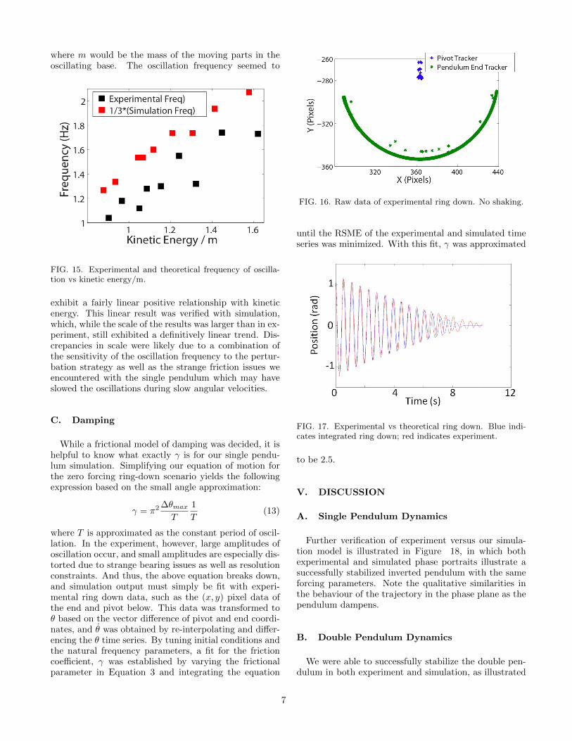
where m would be the mass of the moving parts in theoscillating base. The oscillation frequency seemed to

FIG. 15. Experimental and theoretical frequency of oscilla-tion vs kinetic energy/m.

exhibit a fairly linear positive relationship with kineticenergy. This linear result was verified with simulation,which, while the scale of the results was larger than in ex-periment, still exhibited a definitively linear trend. Dis-crepancies in scale were likely due to a combination ofthe sensitivity of the oscillation frequency to the pertur-bation strategy as well as the strange friction issues weencountered with the single pendulum which may haveslowed the oscillations during slow angular velocities.

C. Damping

While a frictional model of damping was decided, it ishelpful to know what exactly γ is for our single pendu-lum simulation. Simplifying our equation of motion forthe zero forcing ring-down scenario yields the followingexpression based on the small angle approximation:

γ = π2 ∆θmaxT

1

T(13)

where T is approximated as the constant period of oscil-lation. In the experiment, however, large amplitudes ofoscillation occur, and small amplitudes are especially dis-torted due to strange bearing issues as well as resolutionconstraints. And thus, the above equation breaks down,and simulation output must simply be fit with experi-mental ring down data, such as the (x, y) pixel data ofthe end and pivot below. This data was transformed toθ based on the vector difference of pivot and end coordi-nates, and θ was obtained by re-interpolating and differ-encing the θ time series. By tuning initial conditions andthe natural frequency parameters, a fit for the frictioncoefficient, γ was established by varying the frictionalparameter in Equation 3 and integrating the equation

FIG. 16. Raw data of experimental ring down. No shaking.

until the RSME of the experimental and simulated timeseries was minimized. With this fit, γ was approximated

FIG. 17. Experimental vs theoretical ring down. Blue indi-cates integrated ring down; red indicates experiment.

to be 2.5.

V. DISCUSSION

A. Single Pendulum Dynamics

Further verification of experiment versus our simula-tion model is illustrated in Figure 18, in which bothexperimental and simulated phase portraits illustrate asuccessfully stabilized inverted pendulum with the sameforcing parameters. Note the qualitative similarities inthe behaviour of the trajectory in the phase plane as thependulum dampens.

B. Double Pendulum Dynamics

We were able to successfully stabilize the double pen-dulum in both experiment and simulation, as illustrated

7

FIG. 18. Single Pendulum: Experimental vs simulated phaseportraits at stable parameters: A = 10.7 mm, f = 25 Hz.

FIG. 19. Double Pendulum: Experimental vs simulated phaseportraits at stable parameters: 30 Hz for experiment and 100Hz for simulation. Blue trajectory is first pendulum; green isthe second pendulum.

in Figure 19. However, the parameters for stabiliza-tion widely varied from experiment to simulation, andthus so did the behaviour of their trajectories in phasespace. Since both pendula are dependant on each other,it should not very well be expected that one would be ableto exactly recreate the trajectory of the double pendulum

unless the initial conditions and forcing and pendula pa-rameters are well known with high accuracy, which is notthe case here. In this particular experiment, the secondpendulum tended to only slightly oscillate about an an-gle just off-axis of the inverted position and did not crosszero degrees, while simulation showed oscillation aboutthe inverted fixed point for both pendula.

FIG. 20. Top: Illustration of the double pendulum config-urations from time A to time B during a flipping motion.Bottom: Time series of the same flipping motion. Blue seriesis the first pendulum, and green is the second.

A striking behaviour that was periodically observed inthe double pendulum was the separation of stabilizations.When the first pendulum stabilized at either the bottomor the top, the second pendulum could independentlybehave as a single pendulum would behave, giving rise toorientations in which one pendulum could be stable upand the other could be stable down, and vice versa, suchas the flipping example in Figure 20, in which pendulum 1and was initially stable up, and 2 was stable down. Aftera light flick perturbation, the entire pendulum flipped, asdid the individual orientations.

C. Basins of Attraction

In the analysis of the stability of the inverted pendu-lum, it is instructive to see how the basins of attrac-tion change when varying the forcing parameters. I wasable to visualize these basins with the single pendulumSimulink model. The general method is to construct a

8

fine resolution array of initial states in the phase spaceand simulate the model at each of these initial states fora certain amount of time. For every point in this ar-ray, I assign a color corresponding to the final angularposition of the pendulum. I employed the InterpolatedCell Mapping (ICM) algorithm to significantly acceleratethe computation time8. This method only requires thesimulation of the first forcing cycle at each initial state.And with this initial mapping, each initial state will bemapped to another initial state. And thus, one can it-eratively interpolate through cycle by cycle for each ini-tial state for any desired number of cycles. This methodis many times faster than simply integrating the entiretime trajectory at each point. Figure 21 shows a seriesof basins evolving for a 2.72 cm pendulum as the forcingamplitude increases from 0 to 1 cm.

FIG. 21. Basins of attraction for increasing amplitudes. f =50 Hz.

A black pixel corresponds to a set of initial angular po-sition and velocity that settles at the inverted state. Andwhite corresponds to settling at the bottom fixed point.Large expanses of grey indicate initial states that even-tually mapped out of the phase space where no mappingwas initially made, and thus could not be mapped fur-ther, even if the trajectory eventually returned. Stripesand noise indicate spinning modes that have yet to settle.

In determining where these forcing parameters wouldlie in Figure 2, a 50 Hz forcing amplitude with a 2.72 cmrod length would place the frequency in terms of Ω atapproximately 25 based on the natural frequency. The εcoordinate travels from left to right as A increases. It isevident in Figure 21 that at A = 0, the inverted pendu-lum is still in the unstable region. By A = 3, the pendu-lum has passed the lower stability boundary as definedby Equation 4. As the amplitude continues to increaseand approaches the second stability boundary defined byEquation 5, the inverted basin of attraction initially be-gins to dilate, and then elongates and becomes thinner.As this is happening, both basins seem to be rotating andapproaching a vertical configuration in the phase space.I suspect that both basins eventually become perfectly

vertical and infinitely thin as they cross the thresholdinto the spinning modes regime.

VI. CONCLUSION

Our experiments with the inverted pendulum con-firmed that a simple sinusoidal shaking of the pivot isable to stabilize the top equilibrium point. Within thisregion of stability, the frequency of oscillation seemed toexhibit an interesting linear correlation with the maxi-mum kinetic energy exerted by the oscillating base whichwas confirmed with simulation. Previous literature calcu-lated the existence of non-trivial boundaries that definethe regions of stability, instability and spinning in theamplitude/frequency parameter space, which was veri-fied with our experiments of stability boundary maps, ifonly for a small range of frequencies. The evolution ofthe shapes of the basins of attraction as amplitude in-creases provides an illuminating view of how the basinstransition from one region to another as these non-trivialboundaries are crossed.

We verified that a frictional model of damping wasthe most appropriate model for our experimental setup.And as most variations of the pendulum likely use somesort of bearing or surface-to-surface contact, it may bethe preferred model for consideration of damping in mostpendula, at least for simulation purposes. It would beinteresting to study how varying the friction affects thebasins of attraction and the stability boundaries.

We also succeeded in stabilizing the double invertedpendulum in both simulation and experiment. An inter-esting find with the double pendulum was the existence ofseparable behaviour, in which the second pendulum was,to a certain degree, able to act as a single pendulum,once the the first pendulum stabilized. A more thoroughexploration of this phenomenon in both experiment andtheory may be interesting. An unexpected realization oc-curred with the construction of the double pendulum inthat legos are potentially very excellent candidates for alegitimate pendulum setup. Perhaps future students maywant to seriously consider legos if a pendulum projectarises.

Despite the strange bearing issues and rickety con-struction of the double pendulum, there was a shock-ing amount of qualitative congruence between our exper-imental data and the integrations of the simplified andidealized equations of motion. This qualitative agree-ment should serve as a testament to the permanenceand influence of the interesting dynamics found in theinverted pendulum.

REFERENCES

1P. Kapitza, “Dynamical stability of a pendulum whenits point of suspension vibrates, and pendulum with a

9

vibrating suspension,” Collected Papers of PL Kapitza2, 714, 726 (1965).

2R. Grigoriev, “Symmetry and control: Spatially ex-tended chaotic systems,” PHYSICA D , 140(3– 4):171–192 (2000).

3T. Yamakawa, “Stabilization of an inverted pendulumby a high-speed fuzzy logic controller hardware system,”Fuzzy Sets and Systems 32, 161–180 (1989).

4A. A. Gerry K.A. Kramer-F Vanderstiggel Lyons andS. Stubberud, “Control of inverted pendulum systemusing a neural extended kalman filter,” in Proceedingsof the Fourth internation Conference on AutonomousRobots and Agents (2009) pp. 392–397.

5G. G. M. Bartuccelli and K. Georgiou, “On the dynam-ics of a vertically driven damped planar pendulum,” inProc. R. Soc. Lond. A, Vol. 458 (2001) pp. 3007–3022.

6H. N. Gronbech-Jensen James A. Blackburn, “Stabilityand hopf bifurcations in an inverted pendulum,” Amer-ican Journal of Physics 60, 903–907 (1992).

7. R. B. A. Marchewka, D. Abbott, “Oscillator dampedby a constant-magnitude friction force,” American Jour-nal of Physics 72, 477–483 (2005).

8B. Tongue and K. Gu, “Interpolated cell mapping ofdynamical systems,” Journal of Applied Mechanics 55,461–466 (1988).

10