java sea pelagic fishery assessment...

AGENCY FOR AGRICULTURAL RESEARCH AND DEVELOPMENT

RESEARCH INSTITUTE FOR MARINE FISHERIES

~COMMISSIONOF THE EUROPEANCOMMUNITIES

JAVA SEA PELAGIC FISHERY

ASSESSMENT PROJECT

(ALAlINS/87/17 )

AKUSTIKAN I

Workshop Report

Ancol / Jakarta: 5 to 10 December 1994

Edited by : D. PETIT

F. GERlOTTO

N. lUONG

D. NUGROHO

With the collaboration of: P. COTEl

JR. DURAND

P. PETITGAS

Scientific and Technical Document N° 21June 1995

~ AKUSTIKANI _

TABLE OF CONTENTS

SUMMARY 1RINGKASAN 2

TABLES AND FIGURES LEGENDS 6

FOREWORD 9

1. BACKGROUND 11

1.1. General objectives...........................................................•.....................11

1.2. Physical environment ..................................•..•••.•.••.•...•......•.........•......•12

1.3. Cruises : choices and methodology 17

1.4. Equipment and data exploration strategy 18

2. RESULTS 22

2.1. Material and methodology .................................•...•.......•..•...•.......•.......232.1.1. Material. 232.1.2. Data analysis methodology 27

2.2. Synthesis of the results ...................................•..••.•........•...•.........•.......312.2.1. Hydrological results synthesis 312.2.2. Data fihery synthesis 342.2.3. Global acoustic fish densities 342.2.4. Schools distribution 452.2.5. TS distributions 502.2.6. Vertical distribution of the density 552.2.7. Spatial structures 57

2.3. Stratification and evaluation.................................•............•..........•••.....672.3.1. Stratification 672.3.2. Evaluation 79

2.4. Conclusions ........................................................................•..................87

2.5. References 95

3. ROUND TABLE 98

4. ANNEXES 108

4.1. Annex 1 : Workshop announcement. 108

4.2. Annex 2 : Lists of participants .........................•..•.............••...............1114.2.1. Workshop " AKUSTI KAN 1" 1114.2.2. Round table 113

4.3. Annex 3 : Cruises, main characteristics 115

1

~ AKUSTIKANI _

SUMMARY

The PELFISH project aims at a better knowledge of the small pelagie fish stocks

in Java Sea and their exploitation, the ultimate goal being as usual to build a

proper management scheme. To reach this goal one needs to have minimal data

on environment, liable statistic data, knowledge on biology of the main species,

as weil as on socio-economics.

For pelagie resources, acoustic techniques represent a specifie tool which is able

to give very useful informations. Inside PELFISH, it has been used with two main

objectives: at first, repartition and extension of the pelagie resources, and then,

evaluation of the corresponding biomass. It means that the studies have to take

into account the hydroclimatic factors and the seasonal and interannual

variations, which possibly are very important for pelagie recruitments and

production. Later, acoustic data could enable us to understand better the

medium scale repartition of fishes (schooling and dispersion) and their behaviour

towards fishing techniques.

This first report is focused on the general repartition of pelagie fish biomass in

Java Sea; data have been processed during a workshop in Jakarta (5 to 9

December 1994). We used only the ones performed from November 1991 to

March 1994. A more general exploitation of the whole data will-be given in the

next Seminar - AKUSTIKAN Il - which is planned to take place during January

1996.

The main conclusions are the following :

• The sampling methodology has proved itself useful for acoustic stock

evaluations, with a sufficient precision, through the study of two surveys

during two opposite seasons.

• The distribution presents two kinds of gradients : the most prominent is a

West to East gradient, it takes place during the dry season and the main

2

~ AKU5T1KANI _

~

densities are found in the eastern part of the Java Sea. Another gradient is

found from North to South during the wet season.

• The expected precision of evaluation could be around 15%. This low value

must be related to the great regularity of the structures in the area.

• It is possible to propose a biological model of the stratification of the fish

distributions. This global hypothesis is built on the definition of the three

groups of fishes : a coastal group, a more pelagic and widely distributed

group and a dense eastern group.

This contribution to acoustic studies in Java Sea led also to a few

recommendations about processing of other data and/or collection of new ones

in order to improve this first exploitation and also in order to check some

hypothesis : threshold adjustments to have a better discrimination of plankton

biomass ; use of biological information ; more detailed data on coastal stocks ;

evaluation of West Java Sea biomass.

The general conclusion is that the comparison of acoustic results with

bioecological studies of main species, together with fisheries knowledge prove to

be very consistent and the usefulness of echointegration studies is - if it has to

be - fully demonstrated.

3

~ AKUSTIKANI _

RINGKASAN

Proyek PELFISH bertujuan untuk memperoleh pengetahuan lebih baik atas

berbagai stok ikan pelagis kecil dan eksploitasinya. Sedang tujuan akhir adalah

untuk menyusun kerangka manajemen yang memadai bagi sumber daya ikan

tersebut. Untuk mencapai tujuan ini diperlukan data statistik yang dapat

dipercaya, pengetahuan akan bioekologi dari jenis-jenis ikan utama, data

tentang Iingkungan, selain data sosial-ekonomi.

Untuk sumber daya pelagis, tehnik akustik merupakan suatu alat khusus yang

mampu memberikan berbagai informasi yang sangat berguna. PELFISH telah

menggunakannya untuk dua tujuan utama : pertama, distribusi dan penyebaran

sumber daya pelagis, kemudian, evaluasi terhadap biomassa mereka. Ini berarti

bahwa studi tersebut harus mempertimbangkan faktor-faktor hidroklimatik dan

variasi musiman dan tahunan, yang diduqa sangat penting bagi rekrutmen dan

produksi ikan-ikan pelagis. Selanjutnya, data akustik dapat membantu kita

memahami lebih baik penyebaran ikan menurut skala media di mana mereka

berada (pembentukan kawanan dan dispersi serta perilaku mereka) terhadap

tehnik penangkapan yang digunakan.

Laporan ini difokuskan pada penyebaran biomassa ikan di Laut Jawa secara

umum ; data telah diproses selama lokakarya di Jakarta (5 s/d 9 Desember

1994). Hanya sebagian dari informasi yang telah diperoleh selama 15 kali

pelayaran yang telah dilakukan sejak November 1991 sampai Maret 1994.

Eksploitasi terhadap data secara menyeluruh akan disajikan dalam Seminar

AKUSTIKAN Il - mendatang, yang direncanakan akan dilaksanakan pada bulan

Januari 1996.

4

~ AKUSTIKAN, _

~-

Kesimpulan utama adalah sebagai berikut :

• Metodologi penarikan contoh telah terbukti berguna bagi evaluasi stok,

dengan ketepatan yang memadai, melalui studi terhadap dua survei panjang

selama dua musim yang berlawanan.

• Distribusi stok menampilkan dua macam pola penyebaran : yang paling jelas

adalah terdapatnya penyebaran dari barat ke timur, yang terjadi selama

musim kemarau di mana densitas tertinggi ditemukan di bagian timur dari

Laut Jawa. Sedangkan pola penyebaran dari utara ke selatan ditemukan

selama musim penghujan.

• Presisi yang diharapkan dari evaluasi ini mencapai sekitar 15%. Nilai rendah

ini harus dikaitkan dengan kestabilan struktur populasi di wilayah ini.

• Terbuka kemungkinan untuk menyusun model biologi terhadap stratifikasi

distribusi ikan. Hipotesis umum ini disusun berdasarkan definisi dari 3 jenis

pengelompokan ikan yaitu : kelompok pantai, kelompok yang lebih bersifat

pelagis dan tersebar luas, serta kelompok padat di sebelah timur.

Sumbangan pertama dari studi akustik di Laut Jawa mengarahkan kepada

sejurnlah rekomendasi tentang pemrosesan terhadap data Iain yang masih ada

dan/atau pengumpulan data baru agar dapat melakukan pengecekan terhadap

beberapa hipotesis ; pengaturan "threshold" agar dapat membedakan biomassa

plaknton secara lebih baik ; penggunaan informasi biologi dan data perikanan

untuk mengkonfirmasikan model stratifikasi studi tentang pergerakan dan

migrasi ikan ; data beberapa stok pantai yang lebih rinci, dan evaluasi biomassa

bagian barat dari Laut Jawa.

Kesimpulan umum ialah bahwa komparasi antara hasil-hasil dari studi akustik

dengan studi tentang bioekologi terhadap beberapa spesies utama, serta

pengetahuan akan perikanan ini ternyata konsisten dan kegunaan dari studi

echointegrasi - bila harus dikemukakan - dapat ditunjukkan secara jelas.

5

TABLES AND FIGURES LEGENDS

TABLE 1 Statistical values of the Semarang - Matasiri transects (VVest - East) 36

TABLE 2 Evaluation table ••••••••••••••••••••••••••••••••••••••••••••••••••••••••••••••••••••••••••••••••••••••••••••• 87

FIGURE 1 JAVA SEA SITUATION AND MAIN PHYSICAL FEATURES Error! Bookmark not defined.

FIGURE 2 MAIN EQUIPMENTSAND DATA ACQUISITION 19

FIGURE 3 ROUTES FOLLOWED BY THE VESSEL DURING TWO TYPICAL CRUISES 24

FIGURE 4 THE MEAN SALINITIES 32

FIGURE 5 MAIN FISHING GROUNDS 35

FIGURE 6 PROPORTIONAL DISTRIBUTION OF THE FISH DENSITY ALONG THE TRANSECT FROM

SEMARANG TO MATASIRIIN MARCH 1992 (SURVEY 21) 37


MATASIRI TO SEMARANG IN MARCH 1992 (SURVEY 21) 38


SEMARANG TO MATASIRIIN DECEMBER 1992 (SURVEY 27) 39


MATASIRI TO SEMARANG IN DECEMBER 1992 (SURVEY 27) 40


SEMARANG TO MATASIRIIN DECEMBER 1993 (SURVEY 36) 41


MATASIRI TO SEMARANG IN DECEMBER 1993 (SURVEY 36) 42

FIGURE 12 PROPORTIONAL DISTRIBUTION OF THE FISH DENSITY ALONG THE OVERALL

COVERAGE ROUTE IN DCTOBER 1993 (SURVEY 34) 43

FIGURE 13 PROPORTIONAL DISTRIBUTION OF THE FISH DENSITY ALONG THE OVERALL

COVERAGE ROUTE IN FEBRUARY 1994 (SURVEY 41) 44

FIGURE 14 SCHOOLS IN DCTOBER 1994 (SURVEY 34) 46

FIGURE 15 DAY AND NIGHT DISTRIBUTION OF THE NUMBER OF FISH SCHOOLS (N) FROM

10aoE TO 11aoE ACCORDING TO DENSITY, IN OCTOBER 1993 (SURVEY 34) .... 47

FIGURE 16 DISTRIBUTION ON BOTH SIDES OF THE LONGITUDE 112°E OF THE NUMBER (N) OF

FISH SCHOOLS ACCORDING TO DENSITY, IN OCTOBER 1993 (SURVEY 34) 49

FIGURE 17 GENERAL HISTOGRAM OF THE MEAN TARGET STRENGTH IN DCTOBER 1993

(SURVEY 34) ..................................................................................•............ 51

FIGURE 18 REPARTITION OF THE MEAN TS VALUES IN OCTOBER 93 AND FEBRUARY 94 ..... 52

~ AKUSTIKANI _

~

FIGURE 19 REPARTITION OFTHE MEAN TS VALUES IN OCTOBER 93 (SURVEY 34)•••••••••••••• 53

FIGURE 20 REPARTITION OFTHEMEAN TS VALUES FEBRUARY 94 (SURVEY 41) 54

FIGURE 21 VERTICAL PROFIL OF FISH DENSITY ALONG THE TRANSECT FROM MATASIRI TO

SEMARANG ••••••••••••••••••••••••••••••••••••••••••••••••••••••••••••••••••••••••••••••••••••••••••••••••• 56

FIGURE 22 SPATIALDISTRIBUTION ANDVARIOGRAM OF THE FISH DENSITY DURING THE DAYIN

OCTOBER 93 (SURVEY 34) lOlO." 59

FIGURE 23 SPATIALDISTRIBUTION ANDVARIOGRAM OF THE FISH DENSITY DURING THE NIGHT

IN OCTOBER 93 (SURVEY 34) ••••••••••••••••••••••••••••••.•••••••••••••••••••••••••••••••••••••••• 60


FEBRUAR,Y 94 (SURVEY 41).........................•.....•............•.........•••................. 61


IN FEBRUARY 94 (SURVEY 41 ) ••••••••••••••••••••••••••••••••••••••••••••••••••••••••: ••••••••••••• 62


MARCH91 (SURVEY21) ••••••••••••••••••••••••••••••••••••••••••••••••••••••••••••••••••••••••••••••• 63


IN MARCH91 (SURVEY 21) .....•..............••••••.•••..........•••....••••.•••••.......••.....•••• 64

FIGURE 28 SPATIALDISTRIBUTION AND VARIOGRAM OF THE FISH DENSITY DURING THE DAY IN

DECEMBER 93 (SURVEY 36) ••••••••••••••••••••••••••••••••••••••••••••••••••••••••••••••••••••••••• 65


IN DECEMBER 93 (SURVEY 36) ••••••••••••••••••••••••••••••••••••••••••••••••••••••••••••••••••••• 66

FIGURE 30 STRATIFICATION OFTHE SURVEYED AREA 69

FIGURE 31 CURVES OF FISH DENSITY DISTRIBUTION DURING THE DAY AND THE NIGHT IN.OCTOBER 93 AND FEBRUARY 94 .....•...••.•.....••...•.•....••.....••....••.......••••....•...•. 70

FIGURE 32 CURVES OF FISH DENSITY DISTRIBUTION BY STRATA (A, BAND Cl, DURING THE

DAYANDTHE NIGHT IN OCTOBER 93 (SURVEY 34) 71

FIGURE 33 CURVES OF FISH DENSITY DISTRIBUTION BY STRATA (A, BAND Cl, DURING THE

DAYANDTHE NIGHT IN FEBRUARY 94 (SURVEY 41) 72

FIGURE 34 SPATIAL DISTRIBUTION AND VARIOGRAM OF THE FISH DENSITY IN STRAnlM A

DURING THE NIGHT IN OCTOBER 93 (SURVEY 34) 73

FIGURE 35 SPATIAL DISTRIBUTION AND VARIOGRAM OF THE FISH DENSITY IN STRATUM B

DURlNG THE NIGHT IN OCTOBER 93 (SURVEY 34) 74

FIGURE 36 SPATIAL DISTRIBUTION AND VARIOGRAM OF THE FISH DENSITY IN STRATUM C

DURING THE NIGHT IN OCTOBER 93 (SURVEY 34) 75

FIGURE 37 SPATIAL DISTRIBUTION AND VARIOGRAM OF THE FISH DENSITY IN STRATUM A

DURING THE NIGHT IN FEBRUARY 94 (SURVEY 41) 76

7

~ AKUSTIKANI _

~

FIGURE 38 SPATIAL DISTRIBUTION AND VARIOGRAM OF THE FISH DENSITY IN STRATUM B


FIGURE 39 SPATIAL DISTRIBUTION AND VARIOGRAM OF THE FISH DENSITY IN STRATUM C


FIGURE 40 SPATIAL DISTRIBUTION AND VARIOGRAM OF THE SQUARE AVERAGES OF THE FISH

DENSITIES DURING THE NIGHT IN OCTOBER 93 (SURVEY 34} •••••••••••.••••••••••••••• 82


DENSITIES DURING THE DAY IN OCTOBER 93 (SURVEY 34}••••••••••••.••••••••••••••••• 83


DENSITIES DURING THE NIGHT IN FEBRUARY 94 (SURVEY 41) ••••••••••••••••••••••••• 84


DENSITIES DURING THE DAY IN FEBRUARY 94 (SURVEY 41) 85

FIGURE 44 INTERPOLATION (KRIGGING METHOD) OF THE FISH DENSITY IN THE AREA OF THE

CRUISE MADE IN OCTOBER 93 (SURVEY 34) 86

FIGURE 45 REPARTITION ALL OVER THE YEAR FOR (A) GROUP 1 AND (B) GROUP 2 89

FIGURE 46 REPARTITION FOR GROUP 3 (A) IN FEBRUARY AND (B) IN OCTOBER•••••••••••••••••• 90

FIGURE 47 CIRCADIAN DISTRIBUTION OF FISH ALONG THE WEST-EAsT TRANSECT (OCT.) •• 92

FIGURE 48 NIGHT ANNUAL DISTRIBUTION OF FISH ALONG THE WEST-EAsT TRANSECT•••••••• 93

8

~ AKUSTIKANI _

~

FOREWORD

The PELFISH Project which studies the seiners fishing activity in the Java Sea is

sponsored by Indonesia (Agency for Agricultural Research and Development,

AARD), France (French Research Institute for Development through

Cooperation, ORSTOM) and the European Union. Its research is focused on

offshore pelagie fisheries (mainly medium and large seiners fisheries) and its

main objectives are:

• the provision of scientific advice for the future management of

these fisheries ;

• the irnprovernent of the performance of this fishing system in term

of catch, conservation and distribution;

• the evaluation of the socio-economic impact of potential

management measures and technical improvement ;

• the enhancement of fishermen's income.

To reach these objectives, PELFISH has developed three main fields of

activities :

• RESOURCESAND EXPLOITATION

It refers to fisheries functioning as weil as to bioecology or fish populations

dynamics. A special attention is paid to fish behavior and biomass estimation

through echo-prospecting and integration.

• SOCIO-ECONOMIC STUDIES

They evaluate production costs, fish priees, incomes in the fishing sector and

downstream. The research also targets the fishermen conditions of work, the role

of women in the production and the respective weight of the formai and informai

sectors.

9

~ AKUSTIKANI _

~

• TECHNOLOGICAL INNOVATIONS

It is related to nets design and its evolution, the implementation of electronic

devices on the fishing boats, the evaluation of the fish quality and the methods of

conservation.

ln order to have a better transfer of knowledge PELFISH has organized three

Seminars dealing with specifie contents. The first one on BIOlogy, DYNamics

and EXploitation took place in March 1994 and the related BIODYNEX

proceedings are being edited by the Project (POTIER and NURHAKIM, 1995).

"SOSEKIMAft (December 1995) will focus on socio-economics with a special

attention on innovation and management. Then AKUSTIKAN 2 Seminar will take

place in January 1996. The report presented here represents a first glance at

acoustic results before the more global synthesis which will be performed during

the Seminar.

10

1 .

AKUSTIKANI _

BACKGROUND

1.1. General objectives

PELFISH is focused on the exploitation and uses of small pelagie stocks

through "big" seiners fishery. It means that it is a multidisciplinary project

which presents three main fields of activities :

• Biology, fisheries and stock assessment;

• Socio-economic studies ;

• Technological innovations and improvements.

The first description of the objectives was :

u ••••••••• to study and improve the exploitation and the organisation of off shore

pelagie fisheries in the Java Sea, in order to increase the supplY of the

population in quality products and proteins, and to improve the revenue of the

îisnetmen, who make up one of the poorest rural groups. In parlicular, the

project aims at promoting the development of off shore pelagie resources in

the long term, through a better knowledge of stocks (. ..), but also by

suggesting better fishing methods as weil as better conservation, handling and

transformation methods capable of optimizing the profits of both consumers

and fishermen ...".

ln the revised 1990-1994 Work Plan, these objectives were simplified and

clarified as :

• the provision of scientific advice on the management of the fishery;

• the improvement of the performance of this fishing system in term

of catch, conservation and distribution;

11

~ AJ(IJsnKAN' _

• the evaluation of the socio-economic impact of potential

management measures and technical improvement;

• the enhancement of fishermen's income.

It is clear that the objectives of the Project are oriented towards development

and further management. To achieve this, the Project had, first of ail, to gather

the information necessary to get familiar with the environment and the fishing

mode. From these databases we should know the availability of resources to

allow or not some improvements in catches and yields.

The biomass evaluation method by acoustics (echointegration) is the only

method able to supply the necessary information on the condition of stock and

its availability, directly and at any time. That is the reason why it seemed

judicious to use it, ail the more so because, contrary to other world productive

sectors, this method was little used in Indonesian waters, particularly in the

Java Sea (1) • Its use, in the framework of the Project had to aim not only at

evaluating stock but perhaps above ail, at knowing the precise seasonal

variation in the sector where the catch is the most intensive. Knowing the

capacities and the restrictions of the method it was also necessary in the

study, to take into consideration the behaviour of fish so as tc better clarify the

validity of the observations.

1.2. Physical environment (îrom DURAND and PETIT, 1994)

Within an aquatic ecosystem, productivity is deeply dependent on climatic and

physical characteristics of the environment. Thus the level of catches relies

first on specifie characteristics of the ecosystem and then of course on the

(1) ln 1972-1976 thesurveys in the JavaSeawhich seemto havesupplied onlydistribution cards(Venema, 1976); in 1985the PECHINDON cruise, was very localized during onemonth in theCentral partof JavaSea. (Boely et al., 1987)

12

~ AKUSTIKANI _

~

efficiency of the fisheries exploitation. A good understanding of the functioning

of the ecosystem is necessary to conduct a wise management of renewable

living resources. The need for environment knowledge and studies has been

identified by PELFISH initiators from the beginning. Nevertheless it has not

been possible to conduct specifie programs on environment or productivity

issues, which require specifie means and skills. Measurements of temperature

and salinity have been done during the 15 R.V. "Bawal Putih 1" acoustic

cruises we performed from March 1992 to April 1994 (Annex 3). These

horizontal transects and vertical stations allow us to give a good description of

temperature and salinity variations during two successive annual cycles. It

constitutes an important contribution on environment issue since global

studies are quite ancient.

The great Sunda Shelf extends from the Gulf of Thailand southwards through

South China Sea - between Malaysia, Sumatra and Kalimantan - and the Java

Sea represents its south-eastern part (Fig. 1a). It is a large and shallow water

mass. Morphologically, the Java Sea is roughly rectangular. It is weil delimited

on three sides materialized by the western part, it remains nevertheless open

with the Sunda Strait, between Sumatra and Java, giving way to Indian

Ocean, and the Karimata Strait opening northwards on South China Sea.

Obviously the eastern boundary has not the same meaning, as it is wide open

towards the Flores Sea and the Makassar Strait.

This quick description already gives 3 essential features of the ecosystem :

• The discharge of continental fresh water is considerable mainly

from Kalimantan, but also Sumatra and Java rivers. It will explain

partly the low salinities encountered seasonally.

• The seasonal exchanges with South China Sea through the

Gaspar and Karimata Straits should not be underestimated.

13

~ AK~n~NI _

~

' 0 '

100"E 1000E 110"E 1120E 116"E 11BOE

Om 10m SOm 100m 200m 1000m >

Figure 1 Java Sea situation and main physica.l features

a) Sunda Shelf b) Bathymetry c) Toponymy

14

~ AKUSTIKANI _

~

• The eastern delimitation with the South China Sea raise the main

issue : what are the relations with the eastern part of the

Indonesian Archipelago?

We have choosen to define the Java Sea as the area of marine waters - for

depth less than 100 meters - defined by Sumatra, Java and Kalimantan

coasts, the latitude 3° South for Karimata Strait and 4° South for Makassar

Strait (Fig. 1c). Owing to planimetry processing we obtained 442,350km2. In

fact one could ask if near the eastern border the estimation should not include

a large part of continental shelf in Makassar Strait (this northern extension

represent 57,790 km2 above 100 m depth).

The mean depth of Java Sea is about 40 meters and on longitudinal axis, its

bottom is slightly sloping towards east. The maximum is found north of

Madura Island Strait (Fig. 1c). It is interesting to note that there is a clear

dissymmetry between Kalimantan and Java coasts, with shallow waters much

more developed in the northern part than in the southern. Owing to the spatial

definition given above, the deep waters (i.e. more than 50 meters) represent

156,000km2 (about 35% of total area) whereas the coastal shallow ones, less

than 10 m, cover 30,300km2 (nearly 7%).

Many islands and/or coral reefs lie in Java Sea (Fig. 1b), from West to North

East : Seribu, Biawak, Karimun Java, Bawean, Masalembo, Kangean,

Matasiri, Laut Besar. But for the first one, they ail correspond to pelagie fishing

zones. The bottom of Java Sea is mainly - more than 90% - constituted of a

deep layer of dense mud. Near the coast, rocky outcrops associated with coral

formations are observed.

The prevailing c1imate in the Java Sea is a typical monsoon climate marked by

a complete reversai of the wind regime. This phenomenon is caused by

differences in temperature between the continental and oceanic areas. The

rainy monsoon occurs between mid December and March and is

15

~ AKUSTIKANI _

characterised by very windy periods with frequent rainfalls lasting for days.

The dry monsoon occurs from June to September and is more regular. The

climate varies considerably throughout this zone. The winds are the essential

feature of the c1imate. From November to February they blow from the

Northwest with a mean ivelocity of 3 Beaufort. From May to September they

blow from a South or Southeast direction and are more regular, their force

sometimes exceeding 4 Beaufort.

Owing to circulation and salinities, we can consider four types of waters

circulating seasonally in the Java Sea (the last three types are more or less

subject to a mixing) :

• The oceanic water masses coming from the Pacifie and the Indian

Oceans. Permanently present in the Eastern part of the Indonesian

archipelago, they can reach the Java Sea, through the Makassar

Strait or through the Flores Sea. The salinity is more than 34%0.

• "Mixed" waters between 32-34%0, mixed waters from the south of

the China Sea, or oceanic water mixed with rainfalls or streaming in

the Java Sea.

• "Coastal" waters between 30-32%0, Iike the diluted waters from the

south of the China Sea by streaming along the East of Sumatra or

the South Kalimantan borders.

• "River" waters below 30%0 which represent coastal waters more

diluted at the mouth of rivers.

ln reality, there are only two types of original waters in the Java Sea : one

from the west (South of the China Sea), one from the east, oceanic.

The moving and/or the formation of these types of waters is ordered by the

alternative system of monsoon : the wet monsoon from the north-west, the dry

monsoon from south-east.

16

~ AKUSTIKANI _

~

1.3. Cruises: choices and methodoJogy.

Admitting that fishermen operate in the most accessible, rich sectors for

profitability, orienting research towards intensive fishing zones as a priority

was justified. It was just as imperative to know the real extension of these

abondant zones, then their moving according to the seasons.

Let us recall however that the Java Sea has a surface area of sorne 440,000

km2• A sufficiently precise inventory of that area demanded the organisation of

cruises from one to two months, with a ship that was sufficiently fast,

autonomous and equipped. "Bawal Putih 1- at the disposai of the Project did

not present sufficient qualities to insure big surveys. Its indispensable

improvement, its equipment in navigation techniques as weil as in scientific

casting off has been achieved by mid 1993 only. The prospection strategy had

then to be modified by applying to the available knowledge : the possible

existence of an island effect on abundance, the necessary influence of a

gradient in the east-west environmental characteristics on species, finally the

presence of important catches in 'the north east of the Java Sea.

Taking into account the time available for each cruise (autonomy), the best"

way to associate previous facts or hypotheses in 'the prospection was to run a

transect from island to island up to the intensive fishing zone. The duration of

this prospection would moreover permit the carrying out of complementary

observations for the study of local variability, natural behaviour and the one

modified accordinq to practices of traditional fishing, methodological

observations which are indispensable to avoid biases or simply to assure

evaluations (calibration and reverberation measurements in a cage).

It was only once that the sure means of navigation and research have been

acquired that three more ambitious surveys could be carried out; South of the

China Sea : April 1993 and the most extensive prospection possible in the

Java Sea : respectively in October 1993 and February 1994. The calendar of

17

~ AKlJSTlKAN, _

cruises and the types of observations carried out can be found in the

appended document here after (Annex 3).

1.4. Equipment and data exploration strategy.

Besides supplementary navigation equipment (GPS, radar), the

instrumentation of "Bawal Putih ln concerned 3 domains :

1) The automatic acqulrlnq of environmental parameters which is

assured by:

• a L1COR quantameter connected to a data logger (aerial

light) ;

• a surface SEABIRD thermosalinometer (temperature,

salinity) ;

• a SEABIRD profiler for in situ measuring of the temperature,

salinity and Iight penetration from the surface to the bottom.

2) The acquisition of density measurements of flsh completed by.target reverberation measurements.

A dual beam Biosonics 120 kHz echo-sounder permits

the detection of echoes. Two softwares : INES-MOVIES and

ESPTS permit the processing of information stored in two

computers (Fig. 2)

18

~ AKU5TIKANI _

~

PROFILER 1

QUANTAMETER 1

PAPER RECORDER OSCILLOSCOPE

l !

BIOSONICS DUAL BEAMf------'

ECHOSOUNDER

1:1

( ECHOINTEGRA TION 1 (TARGET STRENGTH 1, ,INES MOVIES INTERFACE BIOSONICS INTERFACE

1 lShip'. r: GPS

lOG Shlp'. po.ltion----,

i, , ,COMPUTER N° 1 COMPUTER N° 2

DENSITIES file. AERIAl UGHT file.

Storage PLAYBACK file. TS file.

StorageEVENT rde. /Surface T· .5% .

Profil.. T· .5% .t,

,, , , ,"

OPTICAl CI•••ie Colourecl Cl...ieDISK PRINTER PRINTER PRINTER

(Storage) t Den.ity 1 (Eehogr.m 1 (TS)

Figure 2 Main equipments and data acquisition

11

1 ENVIRONMENT 1

THERMOSAUNOMETER

19

1

~ AKUSnKAN' _

~

1) The sampling of detected fish.

With a bottom trawl (vertical opening 5 m) and a pelagic trawl

(vertical opening 11m) equipped with a netsond (FURUNO)

localizing the position of the net.

The execution of a cruise always takes place according to the same outline:

once the regulated casting off is underway, echointegration occurs continually

during day and night, interrupted only for environmental measurements in

station or sampling (trawls, seiners) following expected planning. Information

on density is provided at each nautical mile. It is not useful to explain in detail

the information which is gathered during a cruise. It will be indicated only that

echointegration supplies three kinds of data 'files, reverberation measurements

and environmental observations, either one file by observation ("stationB

) or by

survey.

Even though this data capture is fairly automated, with the exception of the

sampling, it does not prevent to execute various controls before processing.

That is what can be called the "validation phase", important operation after

which measurements are considered exact. For echointegration, this stage is

carried out through OEDIPE and EXCEL softwares. It consisis on one hand of

controlling the catch of ail parameters, on the other hand of "cleaninq" data so

as to eliminate "noises" : bottom integration, parasites due to superficial

agitation, as weil as due to untimely "meetingB (waves, immersed objects or

undesirable detections such as jelly fish field). It is also during this first work

that the operator takes knowledge of the echogram that informs him on the

distribution variations and allows to collect informations not entirely quantified

(for example, shape of detecting, description of shoals).

The storage of reverberation measurement supplies a priori only average

values. They should be positioned geographically and analyzed in detail if one

wishes to process on elementary measurements. Data from environmental

20

tI.i:JJ AKUSTIKANI _

~

parameters also necessitate processings and are either carried out with the

equipment software or with EXCEL.

The second phase that could be called the formating process will consist in

extracting the needed information from each file (under EXCEL) for graphie or

cartographie representations. This is carried out with OEDIPE, EXCEL,

SURFER, STATGRAPHICS or GEO-EAS softwares.

21

~ AKUSnKANI .....- _

2. RESULTS

INTRODUCTION

The first objectives of acoustic studies in Java Sea in the PELFISH frame were

to operate global surveys of the whole Java Sea. Due to potentialities of the

Research Vessel Bawal Putih compared with the area of java Sea open waters

nearly 300,000 km2- it was quickly understood that our initial strategy was not a

realistic one (cf 1.2. supra). Even with this more restricted design, the volume of

acoustic data was huge and did not allow to undertake in depth processing

during the data collecting phase.

On the other hand we had to identify Indonesian scientists with acoustic

knowledge and skills, in order to have a good transfer of PELFISH results,

results which could find application beyond Java Sea such as the prospection

and evaluation of pelagie resources of major importance in eastem Indonesia.

Ali these reasons led us to organize a workshop where a group of specialized

scientists would gather and process together a first set of data, this work being

the first step to a broader seminar during which a true synthesis could be.attempted. The major theme of the workshop was "Stratification of the Data-

(Annex 1)

ln order to have a wide representation of Indonesian scientists we invited

lecturers and students from various universities : Bogor Agricultural University

and Bandung Institute of Technology rNest Java) ; University of Hasanuddin

(South Sulawesi ) ; University of Pattimura (Mollucas) ; "university of Riau

(Sumatra) ; University of Sam Ratulangi (North Sulawesi) ; College of Fisheries

(Jakarta) (Annex 2A). The Research Institute for Marine Fisheries (RIMF) was

also represented through PELFISH, and ORSTOM sent two specialists

Dr. F. GERLOnO and Dr. P. PETITGAS whose activities and skills have been

particulary appreciated.

22

~ AKUSTlKANI _

~~

2.1. Material and methodology

During an evaluation review in December 1993, F. GERLOTTO (ORSTOM

Montpellier) defined an exploration procedure (GERLOTTO, 1993). One part

of this document enabled us to define the contents of the workshop. Its goals

aim to start up a first data analysis with a view to respond to the most

important objectives defined in our workplan. The carrying out of this analysis

goes through a descriptive stage of the phenomena permitting the answer to

elementary questions: "where" "what" and "which" :

• where are the more productive zones and what are their limits?

• what is the importance of seasonal shifting under the influence of

the environment ?

• which species are these stocks composed of?

The development of this descriptive phase will permit the reaching of the

analytical phase to implement the answer to the question "How rnuch?", The

latter needs a schematization of phenomena ending up with the stratification

of data. That is the reason why the theme "STRATIFICATION- was chosen as

the main goal of the Workshop AKUSTIKAN 1.

2.1.1. Material

Among the whole of the 15 cruises that were available, it was decided to

choose, on one hand, the two surveys covering the most important area of

the Java Sea, on the other hand, three transects from: Semarang to Laut

Besar Islands, the latter being the most frequently prospected to follow the

abundance gradient throuphout the seasons.(Fig. 3a).

For each of these cruises, a data formating was necessary for acoustic as

weil as for environmental data. This work nedeed the "validation " and

23

tt:fJJ AKUSTIKANI _

~

11~ 1120E 114~ 11~

'~ ~~' ';V'/ ~L/~.

11SOE!

i

L

1

r1

i

11lrE11eoE114~1120E,11C7'E100"E

~ ,j (b) ~rr~. Matasirl

r l'~ -'S'~~. . . ~-. ~.; .

aosl~amgl , l 1 1

Figure 3 Routes followed by the vessel during two typical cruises

a) Overall coverage survey in October 93 (survey 34)

b) Transect survey in December 93 (survey 36)

24

~ AKUSTIKANI _

~

"formating" to use adapted softwares. In acoustics, the "validation" and

"formating" need two sets of tools in accordance with echointegration or

with T.S. measurements.

ln echointegration, the principal tool is OEDIPE software. This allows the

correction of the values in accordance with the visual interpretation of

echograms. For various reasons a playback of data can often be used with

the INES MOVIES software. Once this data are validated, OEDIPE allows

the carrying out of sorne succint cartographie works (tracks, positions of

stations... ), and moreover the selection of data files transferable to another

software. At last we used EXCEL software to develop usable files by

analysis software such as EVA, SURFER, LOTUS, GEOAS,

STATGRAPHICS ...

For reverberation data (TS), "validation" does not exist strictly speaking ; the

selection of data under certain criteria demands long manipulations,

impossible to make use of in a routine. The systematic analysis carried out

by the constructor's software has been preferred ; it supplies directly an

average value by station and the distribution of data frequency.

Unfortunately these data are not stored : they have to be manually

keyboarded in the desired format, with the help of EXCEL. •

The description of aggregations in shoals can be carried out by MOVIES B

software. This software was not available at the time of the cruises. An

elementary measure of the shoals then was made manually from

echograms to create "shoals files".

Environmental measurements, essentially temperature and salinity for the

moment are taken automatically from vertical profiles. A software

"SEASOFr supplied by the constructor allows the processing of gross data

transferable to EXCEL. Thus these files can be completed (location) for an

ulterior use.

25

~ AKUSTlKANI _

~

The Iist of databases necessary for the implementation of descriptive phase

can be given succinctly. It necessitates the following types of files, each

with more or less complementary information indispensable according to

the processing treatment (hour, depth, position, date ... ).

ln echointegration :

• Total density

• Density by layer

• Number of samplings

• Number of samplings with detection

• Number of shoals (pelagic, demersal)

• Density of shoals (pelagic, demersal)

• Ali these data are referenced by nautical mile.

For the reverberation :

• Average TS by station

• Average TS by cruise

• TS distribution by station

For environmental data:

• Average salinity by meter by station

• Average salinity by station (the same information can be available

for temperature but this last factor which is very secondary in the

Java Sea is not used).

26

~ AXU5T1KANI _

Caution : during the workshop the densities have been expressed in units

of integration (u.i.) so ail the densities values published in this report should

not be taken as absolute data.

The softwares used for the descriptive and analytical phase are the

following:

• EXCEL (and WINDOWS) to elaborate new files and create

elementary graphs ;

• LOTUS which has the same function ;

• SURFER for cartographie or graphie representation in three

dimensions ;

• EVA which is an analytical software essentially of spatial structure

and modelization (PETITGAS, 1991 ; PETITGAS and PRAMPART,

1993);

• GEOEAS which is a krigeage software and allows the calculation of

the mean and variance on data of which the structure was

modeled.

2.1.2. Data analysis methodology

This procedure stated by F. GERLOnO is the one that, applied to the

results, has permitted during the Workshop to proceed to the descriptive

phase and then led to a tentative stratification through further analysis :

• Description of environmental frame;

• Description of the spatial repartition of density ;

• Representation of distributions (densities and shoals) ;

• Description of the reverberating populations;

27

~ AKUSTIKANI _

• Description of the structures and research of modelization ;

• Analysis of descriptive elements in view of stratification.

Description of environmental frame : the repartition and the Iife history of

population are Iinked to environmental factors. Thus the representation of

general characters of the environment at the moment of cruises is of

primary interest.

This in fact permits one to know quickly the homogeneity level of the

environment and the geographic location of the phenomena which can

potentially act on the abundance or the composition of populations.

Knowledge of the times of change in environmental conditions allows to

situate timing marks beyond which it is certain that the environment has

some repercussion on the inhabitants.

Spatial distribution of densities : this very important point aims first of ail to

locate spatial distribution of the density by cruise, and the global abundance

in order to get known the spatial variations. This description otherwise will

attempt to take into account strictly pelagic or demersal populations (vertical

distribution). The behaviour of detection wm also be taken into account in

this description since it is known that the values on day and night have not

generally the same magnitude ; such a variation between night and day is

then a behavioural indication which indicates a change either of the

composition or of the proportion of species.

The next phase will consist of operating the same observations in the

temporal dimension in order to recognize the seasonal variations.

• Aggregated level

It is a matter of trying to know the level of aggregation of the fish : in fact

fishes are, more or less dispersed. At present, two ways permit the

28

AKUSTIKANI _

description and quantification of this mode of distribution: the proportion of

samplings with fish target and the counting of shoals.

• Structure analysis of density distribution

The populations of fish are not homogeneously distributed. Instead of an

"underdispersion· where densities would be uniform and homogeneously

dispersed, one always observes phenomena of concentration at different

spatial scales (overdispersion). The knowledge of these dimensional

structures is of utmost importance since it will permit a modelling in the

density distribution and then, extrapolation on unprospected zones.

• Species and size

The biological sampling analysis carried out throughout the cruises allows

to attribute measured densities to certain species. This sampling shoutd

otherwise permit the spatial delimiting of each species. It is always

insufficient. The sampling from fishing boats (at sea or at landing points) is

indispensable. Reverberation measurements otherwise supply tirst rate

information. Assuming that the species have approximately the same

reverberation, the measured values of TS permit the evaluation of

respective proportions in size for ail these species.

The analysis of descriptive elements provided by the preceding

observations should permit the stratification elaboration. It is a synthesis

allowing to give zoning hypothesis for the studied area in "strata" having

specific representative characteristics. Their borders are adjusted as weil as

possible since they only rarely coincide with a visible or measurable Iimit.

This stratification will be a tool for a better adjustment of the biomass

evaluation with the contribution of the structural analysis.

This report is the synthesis of the works of the scientists and students

(Annex 2). We choosed 5 acoustic surveys performed in the Java Sea by

29

~ AXUSTI/WIJ _

the PELFISH Project (Fig. 3a.b) selected among a set of 15 surveys

already performed, which are the following :

• Survey 21, performed in March, 1992. This survey is constituted of

a single transect, repeated twice, from Semarang to Matasiri

(harbour-fishing grounds)

• Survey 27, performed in December 1992. This survey has the

same design as the survey 21

• Survey 34, performed in october, 1993. This survey covers the

complete central part of the Java Sea (Fig. 3a), i.e. mainly the area

with depths more than 50 meters and the "Matasiri bank" (part of

the shelf around the Archipelago, with shallow waters (depths less

than 50 m). It includes also the same transect as in surxey 21), not

repeated.

• Survey 36, performed in December, 1993. Same survey as survey

21.

• Survey 41, performed in February, 1994. Same coverage as in

survey 34.

The main objectives of the workshop were to establish a descriptive model

of the exploitable fish populations in the Java Sea through acoustic data

processing, making possible an evaluation of the biomass with confidence

interval. This objectives have been reached through two studies :

• a biological modelling of the Java Sea populations ;

• a characterization of these main populations in terms of spatial and

environmental distribution.

This characterization has been made possible through the study of two

main sets of criteria: environmental and biological.

30

~ AJ<USTIKANI _

Enyjronmental criteria; the fish density distributions have been compared

and related to the main environmental characteristics, such as ;

• sea temperature (surface and profiles)

• sea salinity (surface and profiles)

• morphological characteristics (depth, presence of islands, etc).

Biologjcal criteria; these characteristics were studied on one hand through

the observation of fishery data, and on the other hand using acoustic data,

such as;

• data of acoustic density per ESDU (samplings of 1 nautical mile)

• TS data, average along larger distance (around 2 nautical miles)

• day-night differences in the TS and acoustic densities

• parameters of the schools measured on the echograms and echo

integrator values (density by nautical mile).

2.2. Synthesis of the results

2.2.1. Hydrological results synthesis

It is the most important factor in hydrology, and two seasons are defined,

according the monsoon regime. This is clearly visible on the maps of salinity

average on the water colurnn, drawn from the data .of the surveys 41

(February 94) and 34 (Dctober 93) (Fig. 4a.b).

The distribution of salinity within the two large surveys shows the following ;..

31

~ AKUSTlKANI _

~

100"E

100"E1

108"E1

1000E

110'E

110'E

1120E

1120E

1W'E

1140e

11f>OE

11fiOE

11SOE

11SOE

Figure 4 The mean salinities

a) upper than 34,5%0 in October 93 (survey 34)

b) upper than 33,5%0 in February 94 (survey 41)

32

AKUSTIKANI _

• the marine influence is stronger on the central and eastern parts of

the area studied in October, when the marine waters come from

the east, with salinities above 34.5%0

• the only marine influence in February is observed on the western

part of the area, with salinities above 33.5%0, probably coming from

the Sunda Strait.

The structure of temperatures and salinities show a very regular distribution,

and a low variability, the salinities from 32 to 34.5%0, the temperature from

26°C to 28°C. No thermal or saline front can be observed. Only long range

trends are visible.

The main conclusions about hydrological data are the following :

• The oceanic influence covers mainly the deep area (i.e. depth more

than 50 meters), with the exception of the Matasili bank in October,

which is shallow with marine waters.

• Although it is known from other data (particulary fishery data and

general hydrobiological observations) that the hydrobiological wet

season is centered on March, the brackish conditions are already

visible on survey 41 (February). During this survey there only

remains a small area around Karimunjava Island with salt waters,

on the deep sectors (more than 50 rn),

• The highest contrast between surveys 34 (October 93) and 41

(February 94) appears on the Matasiri bank, which is completely

under oceanic conditions in October and under brackish conditions

in February.

33

~ AKUSTIKANI _

~

2.2.2. Data fihery synthesis

These data come from other parts of the Praject, and include some

observations recorded during the acoustic surveys (Fig. 5).

• Most of the purse seiner fishery is performed in waters with salinity

above 32%0, and the target species is the Layang (Decapterus spp)

• The bulk of the fishery is centered on the Matasiri bank in October

and moves to Lumu Lumu Island in February.

• The catch is twice more important in October on the eastern part of

the Java Sea than in February.

• In April-May no catch is made on these areas.

• The central deep area of the Java Sea suffers a permanent fishery

by the purse seiners, which represents between 9 (February) and

20% (October) of the total catches.

These characteristics of interest in the area under study show that the

Matasiri bank is the most important exploited area during the oceanic

influence, and that the fishery seems highly related to haline conditions.

2.2.3. Global acoustic fish densities

The acoustic values along the transects have been processed for ail the

surveys in different ways. In a first processing, the mean values of density

by day and by night have been calculated for three areas of longitude: west

of 112°E, between 112 and 114°E, and east of 114°E. Then the surveys

have been c1assified according to empirical classes in a single survey, the

lowest stratum representing 1, and the highest 3. On the other hand the 5

whole surveys have been c1assified in the same way, the lowest value

being c1assified as 1 and the highest as 5. These classifications show the

following:

34

~ AKUSTIKANI _

~

118"E11f>OE

~.. -.~

112"E110"E1

10S0E100"E1

Figure 5 Main fishing grounds

80% of the catch in Oct. 93

80% of the catch in Feb. 94

10 to 20% of the catch in Oct 93 and Feb. 94

(Total catch in October twice bigger than in February)

35

AKUSTIKANI _

1) Along the Karimunjava I-Matasiri bank transect.

• There is a great variability in the acoustic mean densities observed

between day and night, the day representing less than the half of

the night, in mean value on ail the data set (Tab. 1).

• Day data : it may be observed a general trend in the density

distribution, the western data being always lower than the eastern

data (Fig. Gb to 11b)

• Night data: two cases may occur:

- in October and December, there is a neat trend in the

density distribution, the west being less dense than the east

area (Fig. Be to 12e) ;

- in February and March, on the contrary, the western and

eastern densities are rather similar (Fig. Ge, 7e and 13e)

Table 1 Statistieal values of the west <-> east transeets

(SM: survey from Semarang to Matasiri, MS : survey from Matasiri to Semarang)

· ' ::U· Survey ..:,):::.:: .. ·21sM 21MS· .,.34sM .:4 1MS ·· " 27SM•• .:27MS) i'.·~6sMt/:36~s

Nùmber::i day 124 222 194 247 204 268 187 172

. ofdata _: :night .. :187 . 209 . :189 .. . 10;: .:) 9.~_ ::: :._ 150 . :__}~ : :::;ii-.: 1 1~)\ I ; ;' ï39.;

Mlnimurn day 153 24 30 26 25 74 82 68

density (ui) night 27 75 ·· 271 164 .· · · 95 . 430 ·. 487 - 94

Maximum day 1341 1291 3750 2548 2445 1643 5552 4925

de~~ity (ui) night . 2345 : .. 1686 · 9850 ...2874' ' 1456 >2972::; : 5769:-::> 3849

Mean day 254 234 1065 330 345 503 1312 942

density{uQ night .- 610 335 2863- -- 1::791-:::-: :.387 : 1333- : 17Eri=-1413

Variance day 75E3 40E3 590E3 150E3 130E3 86E3 134E4 407E3..

night 62E3 56E3 ··334E4 231E3 59E3 ·· 218E3 906E3 658E3

Std. dev. day 0.45 0.86 0.72 1.17 1.05 0.58 0.88 0.68

1mean night 0.98 0.71 0.64 0.61 0.63 0.35 0.54 0.57

36

trI:iJJ AKUSnKANI _

~

100"E

100"E 108"E

1100E

1100E

112"E

112"E

114"E

114"E

11fiOE

11fiOE

11B"E

11SOE

Figure 6 Proportional distribution of the fish density along the transectfrom Semarang to Matasiri in March 1992 (survey 21)

a) Total b) Day c) Night

37

~ AKUSTIKANI _

~

11SOE1

116"E

_.~

114DE

~.. - _.~

112"E110"E100"E1

1000E 100"E 110"E 112"E 114°E 116"E 118"E

_6 ~C)

(a) 1ÇJ 1

1

~C>~

1000E 108"E 110"E 112"E 114°E 116"E 118"E1

6 ~C)

(b)

1000E,

Figure 7 Proportional distribution of the fish density along the transectfrom Matasiri to Semarang in March 1992 (survey 21)


38

~ AKUSTIKANI _

~

11SOE1150E1140E

\)~

r------:... - ~ ~(>9

r-----...• - _ .~

11~E1100E108"E

(c)

(a)p

~o~

1000E 1œoE 11a'E 11~E 114°E 1150E 11SOE

·~w

10001:1

Figure 8 Proportional distribution of the fish density along the transectfrom Semarang to Matasiri in December 1992 (survey 27)


39

AKUSTIKANI _

11SOE11eoE

~.. --~

-------- .. --~

(b)

100"E 1œoE 11(1lE 1120E 114°E 11ee'E 11SOE1 1

.~[)

(a)Ç>

_.~..~ve:-

100'E 108"E 1100E 11ZOE 114"E 11ee'E 11SOE

.~[)

Figure 9 Proportional distribution of the fish density along the transectfrom Matasiri to Semarang in December 1992 (survey 27)


40

~ AKUSTlKANI .....;.",.. _

1000E 1œoE 11CfE 1120E 1140E 11l)OE 11SOE

·~w(a)

o

~oC>

1000E 108"E 11CfE 1120E 114DE 116"E 11SOE

·~w(b)

t>

~oC>

1œoE 108"E 11CfE 1120E 114DE 116"E 11BoE1

-:(c)

Qt>

_.~..~oC>

Figure 10 Proportional distribution of the fish density along the transectfrom Semarang to Matasiri in December 1993 (survey 36)


41

~ AKUSTIKANI _

~

1000E 100"E 11CJ'E 1120E 114°E 11f50E 11SOE1 1 1

·~W

(a)

p

~v~

1000E 100"E 11CJ'E 1120E 114"1: 11f50E 11SOE

·~W

(b)

~@) p

c::?

_.~..~C>~

1000E 100"E 11O'E 1120E 114"1: 11f50E 11SOE1 1

·~W~

(c) .la

_.~..~v~

Figure 11 Proportional distribution of the fish density along the transectfrom Matasiri to Semarang in December 1993 (survey 36)


42

~ AKUSTIKANI _

~

11SOE1150E1140e11Z'E110'E1000E1000E1

ff'>-'-----------...::....----------L--------"'---~1œoE 1000E 110'E 11Z'E 1140e 1150E 11ffE

ao~---------.::>.----------L--------"'---~

Z'\>-r<:::-::-~----'-----'--r-------L------L...----'--...,..._-,-"'--__r_

Figure 12 Proportional distribution of the fish density along the overallcoverage route in October 1993 (survey 34)


43

~ M~~NI _

~

100'E 1œoE 110"E 112"E 114°E 11f>OE 118"E1

1

~(a)

\) ~

C>

i

cJ~v 1

D

100'E 1œoE 110"E 112"E 114°E 11f>OE 118"E2" 1

1

~i

(b) rf>O C>

~(>98"

100"E 108"E 110"E 112"E 114°E 11f>OE 118"E2" , 1 1

·~w(c)

c> 11

~

~C:>Î

Figure 13 Proportional distribution of the fish density along the overallcoverage route in February 1994 (survey 41)


44

~ AKUSTIKANI _

~

2). Considering then the two large coverage (October and February),

several observation can be made:

• October: a general important gradient can be observed from west

to east, the western data being lower. The central area data (within

the 50 m deep area) are higher than the south coastal area. No

gradient can be pointed out on the north-south direction (Fig. 14).

• February: no gradient in the west-east direction. Centre of the area

with densities lower than in the south-north gradient (Fig 15).

2.2.4. Schools distribution

School data have been studied only for survey 34 (October 1993), and the

main results cannot be extrapolated to the whole data set. Nevertheless

interesting pieces of information can be obtained from these data. Different

school parameters have been studied :

• their relative density (echo integration of a single school) ;

• the spatial distribution of the schools. Two categories were made:

demersal and pelagie;

• their vertical distribution in the water column.

From this data set several main conclusions have been Iisted :

• Benthic schools can be observed scarcely in the area, and obiously

concentrated in the eastern part, east of 114°E (Fig. 14b).

• On the contrary, pelagie schools are mainly distributed in two

areas. The first one appears at the western Iimit of the survey area,

west of 111°E. The second one is observed at the east of the

survey area, and particulary on the Matasiri bank and the 50m

depth area (Fig. 14a,c). This second area is the most important.

" 45

~ AKUSnKANI _

~

11SOE11eoE11Z'E1100E10s0E

@1000E 1000E 1100E 11Z'E 11401: 11eoE 2500

· ~C) density (ui)

(b) ....0 Il

0 o

oÙ~C)

10001: 1000E 110CE 1120E 1140e 11eoE 118"E1

· ~C)

(c)

&>

~oC)

Figure 14 Schools in October 1994 (survey 34)

(a) Distribution of the Pelagie sehools(b) Distribution of the Demersal sehools(e) Areas of the main pelagie sehools concentration

46

~ AKUSnKANI _

~

60 CDay1080 < Longitude < 1100

.Nlght40

N

20

00 100 200 300 400 500 600 700 800 900 1000

denslty (u.l)


.Nlght

N 20

00 100 200 300 400 500 600 700 800 900 1000

denslty Cu.l)

60 CDay11r < Longitude < 1140

.Nlght

40

N

20

00 100 200 300 400 SOO 600 700 800 900 1000

denslty Cu.!)


.Nlght

N 20

oL--....,L..-.L--.,l-JI.......-,I;~..e::a- .=... _

o 100 200 300 400 500 600denslty Cu.l)

700 800 900 1000

201160 < Longitude < 1180 CDay

.NIght

N 10

oL--....L..-.L--.__II.c;;:~~__Io_I_..r;;~ _'_.L...o

o 100 200 300 400 500 600denslty Cu.l)

700 800 900 1000

Figure 15 Day and night distribution of the number of fish schools (N)from 10Soe to 11Soe according to density, in October 1993(survey 34)

47

AKUSTIKANI _

• The histograms of density of the schools have been calculated for

the five strata: 108-110oE ; 110-112°E ; 112-114°E ; 114-116°E

(Fig. 15). The same distribution inside two main areas can be

observed : the highest number of schools is present in the east.

Dense schools can be observed both in the east and the west, but

no dense school is present in the central area (from 112°E to

114°E).

• The histograms for two main areas (west and east of 112) are

slightly different in their high classes (Fig. 16). A common mode

appears ail over the area between 50 and 150. A second mode is

important in the east (mode 200-500). Although less important, it

can be seen also at the west. On the contrary, a third mode of

dense schools (above 1000 in relative units) is observed at the east

of 112°E, and is absent in the west.

• The echo integration values for the schools only have been

calculated in the ESDUs prior to the workshop. The variogram on

this variable at this scale shows no spatial structure as it stays fiat

up to 50 nautical miles.

Concluding the study of schools, one can say that fish in schools are

present in small densities ail over the area, with sorne differences in the

spatial distributions according to their nature (pelagicldemersal) or their

densities. A general gradient from west to east can be noted as far as

school number is concemed, but in the other parameters, the distribution is

not so simple, sorne structures being concentrated in the west of 112°E,

ether at the east (Fig. 16). The 112°E line seems to be in sorne occasion a

natural "border" between two kinds of structures.

48

AKUSTIKANI _

1080 < Longitude < 112"

10090

807060

N 50

40302010o

o 100 200 300 400 SOO 600

Denstty (U.!.)

112"< Longitude < 11SO

700 800 900 1000

70

60

50

40N

30

20

10

oo 100 200 300 400 500 600

Denslty (U.I.)

700 800 900 1000

Figure 16 Distribution on both sides of the longitude 112°E of the number(N) of fish schools according to density, in October 1993(survey 34)

49

AKUSnKANI _

2.2.5. TS distributions

The Target Strengths have been measured using a dual beam echo

sounder ail along the surveys. The data of February (41) and October (34)

have been studied in detail. The TS values represent the mean value of a

large set of measurements during 1 to 3 miles along the transects. Thus

their representativity is good, but the actual histogram of TS cannot be

known for a particular area. The global histogram for survey 34 has been

made (Fig. 17).

The transformation of the TS values in weight is not yet available inside the

results of the Project, although methodological measurements have already

been made. As an indication we give the values of fish length versus TS

from the equation of Love (1974), and a point value measured within the

Project (Fig. 18 to 20).

The following observations can be pointed out:

• The mean TS are higher in October than in February.

• The high TS are distributed ail over the area in October, but almost

ail of them belong to the deep area (> 50m) or the Matasiri bank in

deep sea (border of the shelf at 116°E, and in the center of the 50

meters area at 113°E) (Fig. 18).

• TS are higher in waters> 50 m in October as weil as in February

(Fig. 18).

• The day-night variability seems typical of surveys : the night TS are

higher than the day TS in October, and seem sirnilar in February

(Fig. 19 and 20).

50

AKUSnKANI _

16

14

F 12

re 10

qu 8en 6cy 4

2

-56 -55 -64 -53 ~ -51 -50 -49 -48 -47 -46 45 -44 -43 42 41

T.S.

Figure 17 General histogram of the mean Target Strength in October 1993(survey 34)

51

~ AKUSTIKAN , _

~

11SOE1150E11~E1100E.

g ce ,) ~) co___e-'

o .....'wo

10a0E1000E~S--r=-:;--"'_T_----J'----'-,._------.L------l----..l.-.,.___,_-.L.-_____.,._

~· ·.W4°S )

. (a)

L

1000E 10a0E 1100E 11~E 114°E 1150E 11SOE~

, .i:t f\r"

4(b)

50S-

,-.....-:».......................... '- )

-~

1

Figure 18 Repartition of the mean T5 values in October 93 and February 94

-56.56 < 0 < -49.84 < 0 < -48.63 < < -47.92 < • < -46.53 <. < -40.89

a) October 93 (survey 34) b) February 94 (survey 41)

52

~ A_~NI _

1000E 10s0E

(a)

1100E1

11;20E

o 0o

' 0o ~ 0

11e>E 11SOE

r:\

11SOE1

11e>E1

11;20E1100E10s0E

.' ~D.W'../

1000E

SOS-.l----,,..------,--------r------r----.,.--L------r--~-__,____--L

Figure 19 Repartition of the mean T5 values in October 93 (survey 34)

-55.12 < 0 < -50.55 < 0 < -49.48 < < -48.45 < • < -48.02 <. < -46.21

(a) Day values only (b) Night values only

53

~ M~~NI ~~

1000E 1000E 11a>E 11ZJE 114°E 11SOE.\

1 1l

1 r.~

~ ~4

(a) 00

00 cV ~

t> 0

•

1_~sos D

1000E 1000E 11a>E 11ZJE 114°E 11SOE 11aoE·ZJ

~" {)1

~

'~0'~.(b) •

0

• ...~ ~

0 t>

aoS...L-------,r-- - --.--- - ~------;r----y-~-

Figure 20 Repartition of the mean TS values February 94 (survey 41)

-55.12 < 0 < -50.55 < 0 < -49.48 <

(a) Day values only

< -48.45 < • < -48.02 <. < -46.21

(b) Night values only

54

~ AKUSTIKANI _

~

• when observing the variograms of the total mean TS data for

surveys 34 and 41, one may note a long structure (between 60 and

100 miles, which seems closely related to the distribution of the big

fish inside the waters more than SOm depth (approximately same

dimensions). More detailed research is needed, in order to

evaluate the time (day-night) effect.

The main conclusions on the TS analysis are:

• There is a trend in the fish length towards the longitude: TS are

smaller in the west than in the east of the area.

• There is a probable trend towards the depth or latitude, fish

remaining in the deep area of the Java Sea are bigger than fish

outside ofthis area (except Matasiri bank in October).

• The fish migrate within the year, the big fishes being close to the

eastem border of the shelf or outside the area in February, while

they are present in a large portion of the area in October. The

migration way could follow the movements of the water mass,

inside the salted waters, Le. along the deep area (more than 50 m

depth).

2.2.6. Vertical distribution of the density

The vertical distibution has been difficult to observe using the data set, and

a few preliminary works have been done along the west-east transect on

several surveys (Fig. 21).

55

~ AKUSnKANI _

~

Om

10

P 30th 40

'--_ Bottorn line(a)

' l ' Il Il,1....."~I ••I I.II~

20

50

70

60

De

Matasiri • Semarang

Om

~ .'+111 f 1 .1.'lt~ 110 --+10

+*. '*, -.. , t-

D20

~'IIMI'e . . l ' ••114 I~P 30t

'i'1. ' • ,. • ... 'h 40

50

60(b)

70 Bottom line

80

Figure 21 Vertical profil of fish density along the transect from Matasiri toSemarang

(a) December 93 (b) February94

56

~ AKUSTIKANJ _

For several reasons vertical distribution is indispensable to study :

• the fishery exploits a "semi-demersal" population attracted with

Iights : the evaluation of the parts due to pelagie and demersal

populations is important.

• the high difference between day and night data (densitles, TS)

makes it impossible to study together those data. An interpretation

of the ressons producing thèse differences is needed.

The study of these distributions is difficult to do. Nevertheless some other

observations show several points of interest that should be more

documented :

• Two populations are present at the same place : one which

remains pelagie more or less ail the time (day and night) ; one

which disappears during the day and is present as pelagie during

the night.

• There is an important circadian cycle in the density measurements.

The biomass increases suddenly at around 6:00pm and decreases

at 5:00am. These short periods must be better known.

• The horizontal layers are traversed by the population which is

moving upwards during the night : this population can be seen in

the deepest layers at the beginning of the night and in the

shallowest ones at the end.

2.2.7. Spatial structures

Spatial structures have been characterized by computed variograms. The

variogram is the measure of variance between points which is function of

the distance separating them. It enables to dissect the total data variance

57

~ AKUSTIKANI _

~

spatially into correlation variability occuring at different scales. The main

parameters are :

• the sill : it is the maximum level of variability between points. It can

be higher than the data variance.

• the range : it is the distance at which the sill is reached. it

measures the average diameter of the area of influence around

each point.

• the nugget : it measures a heterogeneity in the spatial distribution.

For instance, if high and low values are very close neigbours, the

nugget would measure the variance associated with this

discontinuity.

A structure is characterized on the variogram by an increase in the curve,

Le. doser points are more similar than distant ones. The experimental

variogram may show different structures for different scales of distances.

Each one corresponds to a partition of the data variance. The experimental

varioçram must cross the data variance.

Variograms have been computed on the surveys available for the workshop

(Fig. 22 to 29). Day and night data have been separated and a variogram

computed on each sub data set. Night data are on average higher than the

day data. Thus, on the entire data set, the night data generate artefactual

structures with a range equal to the distance sailed during the night time.

Sorne structural characteristics stay constant for ail surveys. This means

there is a structure which is constant from one year to the other, from one

season to the other and during one season.

58

~ AKUSnKANI _~

Data parametersNumber: 936mean: 985var: 6.1E5std/m: 0.79

1l8.98 nO.78 112.S8 114..38 IIb.18108.08 1O'.l.88 11tr.8 113.68 115.28

OEDf>

Variogram parameterslag number : 120lag: 1tolerance : 0.5

O.OEO~--.--.................__._-...........~___._- ...........~-I12.00 36.00 bO.OO 86.00 108.00

00.00 26.00 68.00 72.00 % .00 12

Figure 22 Spatial distribution and variogram of the fish density during theday in October 93 (survey 34)

59

~ AKU5TIKANI _

~

.8

108.97 110.73 llZ.19 11l.Z5 116.01108.09 109.&5 llUl 113.37 115.13

fil~.OEOb •

~5XO~ r~'l.OEO~ é :3.5EO~ tf! ~fil ,i,~ Cl~

.~ :...~ fil If' al ~

3.0EO~ fil : 'OATi"l~ ri ~~5EO~;@ l' ~ ~ ~ 1 e

~'~ el

: ~~ e(VW!\ii t&,OE06l

5.0EOo;.~

o.o~12.00 36.00 60.00 8l .00 108.00

00.00 2t.00 lB.OO noo 96.00 12

Data parametersNumber: 689mean: 2744var: 3.5E6std/m : 0.68


Figure 23 Spatial distribution and variogram of the fish density during thenight in October 93 (survey 34)

60

~ AKUSTIKANI _


108.'31 110.75 112.53 \tl .31 116.09IOS.0S 109.S6 nl.6l \t3.l2 115.20 11

Variogram parameterslag number : 120lag : 1tolerance : 0.5

12.00 36.00 60.00 SUO 10S.0000.00 2l .00 lS.oO 12.00 %.00 12

Figure 24 Spatial distribution and variogram of the flsh density during theday in February 94 (survey 41)

61

~ AKUSnKANI _

\

r Data parametersNumber: 825mean: 1040var: 5.1E5std/m : 0.69

03 .98 nO.78 112.58 1108 116.1803 .08 m .88 msa 113.'8 11528

12.00 36.00 GO.OO . 8(.00 108.0000.00 2'.00 (8 .00 72.00 % .00 12


Model parametersmodel1spherical (sil! 2E5 ; range 84)model2Spherical (sill2.8E5 ; range 12)

Figure 25 Spatial distribution and variogram of the fish density during thenight in February 94 (survey 41)

62

~ AKUSTIKANI _

~

111.81 112.~1 114.01 115.111112& 112.3& 113.4& 114.5&

Data parametersNumber : 186mean: 251var: 6.1E4std/m : 0.99

4E05 ~~~ \

:',Q ljl2E05 :':Q ,1

lE05 :.~ ~~ ltJ ljllirSJ l', 1 .'.

~:~:: m l ~ Qg,:~1 1 :e' ~

8~E~ : ~~~

7.0E04 :' a,6.0EO III

5.0EO J1~9 (;JQ ~

~OEO n ~..~f1#k~ ~~~ri,~j.~ :3.0EO @'fiFt;.~ v ~~ r~"lffi ~ @il2.0EO rD

OEO BO.OEO~::::=;==F=;====:=~~~~-~~-~-l

10.00 30.00 50.00 70.00 ~O.OO

00.00 20.00 40.00 &0.00 80.00 10


.OEOI

~.OEOI

13·0Eol

~OEO'I )

OE~ If

Model parametersmodel1spherical (sill 2E4 ; range 12)model2Spherical (sill 2E4 ; range 4)

30.0020.00

10.00O.OEOI()l----~---~---~---1

00.00

Figure 26 Spatial distribution and variogram of the fish density during theday in March 91 (survey 21)

63

~A_~NI _


06.16

110.65 111.37 112.09 112.81 113.53110.29 l1tOl rn73 llH5 113.17

11:06

OE06

Q11·,··~""'."'.

m:...::.Q , ~

~ m:I\Q. 1..~ tl:~~ - ,

O.c1 rI!~\IP.lJ.;...ee 1:lJ'" el

, ,


10.00 30.00 50.00 70.00 90.0000.00 20.00 '0.00 60.00 80.00 10

Q""·.·., .·

OEOS

,. ,, ., ,'.e

Q", ., .,

~ : '0. , '", ,.,'.~

Q,rJ Il...1. : Q. ., ." ,., .,. ."el

Model parametersnugget : 2.8E4model1spherical (sill 3E4 ; range 15)model2Spherical (sill 2E4 ; range 3)

20.0010.00

. 0EO(}j.-----~-----~---1

00.00

Figure 27 Spatial distribution and variogram of the fish density during thenight in March 91 (survey 21)

64

~A__NJ _


nO.73 russ m .05 114.21 115.37110.15 nt31 112.47 113.~ 114.79 11


Figure 28 Spatial distribution and variogram of the fish density during theday in December 93 (survey 36)

65

~ M~n~NI _

~

05.5

05.71

Data parametersNumber : 135mean: 1784var: 8.9E5std/m : 0.53

110.73 111.61 112.19 113.37 111.25110.29 11117 112.05 112.93 113.S1

05.71

05.5~

OS.6~

05.1

fo5.S9

os.u

-05.3~

Œ06

SE06

5E06

.2E06

Variogram parameterslag number : 120lag: 2tolerance : 1

HEO&c1,····~ ~; ~~~ ::: ~6~ ~': ~ ~: ~ Q:!lj: @ :,:i~ ~ ~~ : m l!l'

Jh' ~ ~~.OEO" Gl ~~ ~~ ~~ ~, l!l

~.OEO" r ~ 0

@ 0 ,

p.OEOS ~ , ~

p.OEO ~ -~21.00 72.00 120.00 16S.00 216.00

00.00 IS .OO % .00 lU.OO 192.00 2

Figure 29 Spatial distribution and variogram of the fish density during thenight in December 93 (survey 36)

66

~ AKUSTIKANI _

• the coefficient of variation is very low, inferior to one generally

• the nugget effect is very low, always inferior to 10% of the data

variance (Iow local variability)

• day and night structures are very similar

• a small scale structure with a range varying fram 5 to 20 nautical

miles is present on ail surveys

• a trend in zone means at the regional scale generates an increase

on the variogram at long distances, larger than 50 nautical miles.

This trend is oriented west-east during October 1993, as higher

densities stand on the Matasiri bank. This trend is oriented south

north during February 1994 during the day because of higher

densities near the Java coast. The small scale structure has a

varying range.

When the long range structure is not present in the data, variance is

reached at the sill of the small scale structure. This is weil seen in the

survey 21 (March 91) because night sampling stayed in the middle of the

Java Sea (Fig. 27).

The data variance can be split into variance due to the nugget (small),

variance due to the small scale structure and variance due to the long

range regional trend (or structure). On the average, half of the variance

occurs at small range and the other half on the long range structure.

2.3. Stratification and evaluation

2.3.1. Stratification

The main interest of stratifying an area is to better describe each single

strata and the decrease of the variance. When a stratification can be drawn,

67

~ AKUSTIKANI _

~

a particular knowledge of the biology and ecology of the population or

community is obtained, and the variance due to the artificial Iink between

two independent zones is not added anymore to the data.

The 5 surveys have given a large set of information that allows an attempt

to stratify the area. We have seen in particular that three main groups were

present in the area of study :

• a group clearly identified as a south coastal group, mainly recorded

close to Semarang, and on which very few sampling has been

done (group 1) ;

• a group scattered ail over the area, with a permanent kind of

structure at small scale (around 10 nautical miles), with pelagie

schools and low dispersed densities (group 2) ;

• a dense group on the east, which suffers the most important part of

the fishing exploitation, and may migrate from the area and thus,

can disappear at some periods of the year (group 3).

ln these conditions it seems reasonable to stratify the area in 3 strata,

which have been defined as follows (Fig. 30):

• Stratum A : south of 6D20'S and west of 114DE

• Stratum B : north of 6D20'S and west of 114DE

• Stratum C : north of 6D20'S and east of 114DE

Once the stratification is defined, one can test whether the distributions

inside each stratum are homogeneous and particular. This has been done

by calculating means and standard errors in the strata by day and by night,

by drawing the histograms of density distribution, and by calculating

variograms in each of them (Fig. 31 to 39).

68

~ AKUSTIKANI _

~

100'E 108"E1

110'E 112"E 114°E 116"E 118"E

Figure 30 Stratification of the surveyed area

~ Stratum A: Coastal population

0IIllIIJJ Stratum B : Neritic population

~ Stratum C : Oceanic population

69

!i!:Jj AKUSTlKAN ' _

October 93 (survey 34)

160

140

F 120re 100qu 80en 60cy 40

20

0

0

450

400

F 350

r 300e

q 250ue 200

nc 150

y 100

50 ,0

0

---Day

- Night

.. . ...~ . .-

...... - '

1000 2000 3000 4000 5000 6000 7000 8000 9000 10000

Denslty (u.l)

February 94 (survey 41)

---Day

- Night

". ..1000 2000 3000 4000 5000 6000 7000 8000 9000 10000

Density (u.l)

Figure 31 Curves of fish density distribution during the day and the night inOctober 93 and February 94

70

~ AKUSTIKANI _

October 93 (survey 34)Stratum A

---Day

• Night

. - .1000 2000 3000 4000 5000 6000 7000 8000 9000 10000

Density (u.l.)

O I--i---+-' -.;;.....__""- _

o

80

y

F

r 60equ 40e

n 20c

October 93 (survey 34)Stratum B

---Day

• Night

".. .."

100Fr 80eq 60ue 40nc 20y

1000 2000 3000 4000 5000 6000 7000 8000 9000 10000

Density (u.l.)

October 93 (survey 34)Stratum C

20

60Fre 40quency

___Day

_ Night

'" "__ 1 ,,,,,,"

---.---..... .. - ... ' , ..1000 2000 3000 4000 5000 6000 7000 8000 9000 10000

Denslty (u.l.)

Figure 32 Curves of fish density distribution by strata (A, Band C), duringthe day and the night in October 93 (survey 34)

71

@ AKUSTIKAN 1 _

~

Figure 33 Curves of fish density distribution by strata (A, Band C), duringthe day and the night in February 94 (survey 41)

72

~ AKUSTIKANI _

0

0

0 8 Data parameters0 0 Number: 49

0 (0 mean : 2069OG.3 0 var: 7.5E5

std/m : 0.42

OG.3 0o

OG.3 lO~ .G' 110.20 110.7G 111.32 111.8810~.3G 10~.n 110.'8 111.0' 1II.GO

GEOG

.'EOG

12EOG

OEOG

18.0EO·

. OEO~

~.OEO~

OEO'

Q1

".'"".', '.', '

ci :,

IlGQ,

à~

, Qfu :~'e~ : 1.

1 0 ~

'~' 0

Variog ram parameterslag number : 100lag: 1tolerance : 0.5

~.OEOI~---r-----,...---~---I

00.0010.00

20.0030.00

Figure 34 Spatial distribution and variogram of the fish density in StratumA during the night in October 93 (survey 34)

73

~ AKUSTIKAN 1 _

~

••Data parametersNumber: 442mean: 2111var: 2.1E6std/m : 0.69

108.82 110.02 1tt22 112.42 113.t2108.22 109.42 110.t2 111.82 113.02


Model parametersmodel1spherical (sill 1E6 ; range 5)model2Spherical (sill 1.3E6 ; range 25)

10.00 30.00 50.00 70.00 90.0000.00 20.00 40.00 tO.OO 80.00 10

Figure 35 Spatial distribution and variogram of the fish density in StratumB during the night in October 93 (survey 34)

74

~ AKUSTIKANI _

~

115.16 11S.46 115.76 116.06 116.36115.01 115.31 115.61 115." 116.21 1

I7.2EO&

~.4EO&

~.6EO&

10.00 30.00 50.00 70.00 ~O.OO

00.00 20.00 40.00 60.00 80.00 10



00.00 20.00 40.00

Model parametersmodel1spherical (sill1.3E6 ; range 4)model2Spherical (sill 1.2E6 ; range 15)

Figure 36 Spatial distribution and variogram of the fish density in StratumC during the night in October 93 (survey 34)

75

~A~~NI _

.5E05

OEO~

3.5EO~

3.0E05

109.39 110.35 111.31 112.27 11323108.91 109.87 110.83 111.79 112.75 11

5.0E05 f~i.5EO~ : 0

.OE05 I!I··,·Jl,

o •;; ~

o :~

5E05 lè~9h~~Q,1e~l;t~~Q~~ ~OE05 riJ ~'u 8~

~.OEO'- ri13

~.OEOI}j--~-~-~-~-~-~- 1

Data parametersNumber: 123mean: 1633var: 2E6std/m : 0.27


Q."'..,

00.00

8E05

00.00

10.0020.00

30.00

20.00

tO.OO50.00

&0.00

~~.'.':~~::0 r!),,,

: Q :

~~ ~, , '~.~ ,

'~

tO.OO

Model parametersmodel1Spherical (sill 1.4E5 ; range 8)

Figure 37 Spatial distribution and variogram of the fish density in StratumA during the night in February 94 (survey 41)

76

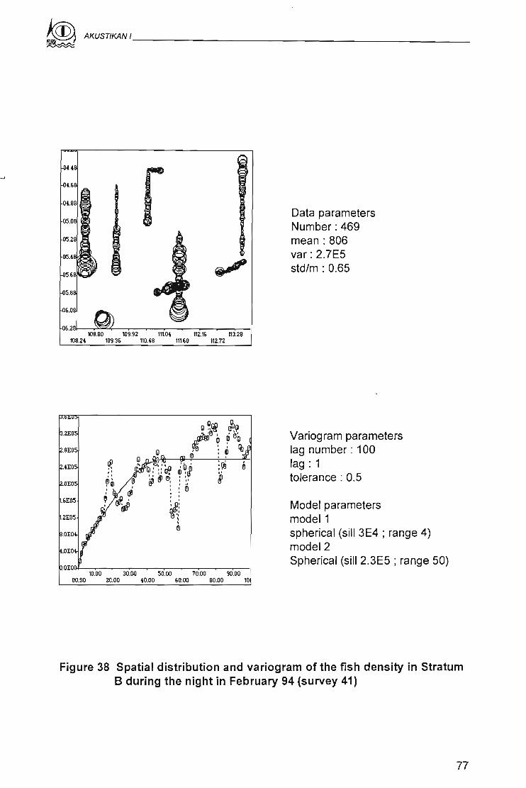
~ AKUSTIKANI _

Data parametersNumber: 469mean : 806var: 2.7E5std/m : 0.65

108.80 109.92 I1t04 112.1& 113.28108.24 109.3& 110.48 111.&0 112.72


Model parametersmodel1spherical (sil! 3E4 ; range 4)model2Spherical (sill 2.3E5 ; range 50)

10.00 30.00 50.00 70.00 90.0000.00 20.00 40.00 &0.00 80.00 10

Figure 38 Spatial distribution and variogram of the fish density in StratumB during the night in February 94 (survey 41)

77

~M~~NI _

05.5

OS.7t

05.95

06.16


06.31

06.58

11(.83 115.25 115.67 116.09 116.51llH2 115.0t llS.t6 115.88 116.30 116.

12-2E06

~.OE06

8E06

.6E06

.tE06

.2E06 Q Q:~ nll

OE06" Q':!'"__ '\ .,,;(9

8.0EO~ .',

.OE05 [ ~~~ri1~m, (Jl .,e mt.OEO~ g ~

2.0E05~

O.OEOOj.I!l_~--'--_~--,--~_~~_"---.--_110.00 30.00 50.00 70.00 90.00

00.00 20.00 tO.OO 60.00 80.00 10


00.00 20.00

Madel parametersmodel1Spherical (sill 7E5 ; range 14)

Figure 39 Spatial distribution and variogram of the fish density in StratumC during the night in February 94 (survey 41)

78

~ AKUSTIKANI _

From these pieces of information, several conclusions may be considered.

• The stratification seems reasonable, and the results inside each

stratum correspond to what was expected : important difference

between Band C in October (presence of the group 3 in C,

Fig. 32) ; similarity in February (absence of group 3, Fig. 33) ;

similarity of day values in ail the strata ; strong differences between

night values.

• The variograms show no nugget effect, but a structure which is

very similar to those of the general variograms : that means that

the small structure is observed everywhere (Fig 34 to 39)

• The histograms show again the specificity of the three strata and

the representativity of the 3 main groups.

From these observations two facts have to be pointed out:

• The longitude border between the strata (114°E) is not very c1early

defined, and as there is no front but only long range trends, no

totally satisfactory limit will be drawn according to the longitudinal

dimension.

• There is very few samples in the coastal area, which remains

almost unknown, and needs some additional pieces of information.

2.3.2. Evaluation

Acoustic surveys of fish populations enable to derive instant estimates of

biomass. These values cannot, a/one, be helpful for fishery management.

Acoustic biomass estimates have two major sources of uncertainty : spatial

error and conversion error.

79

~ AKUSTIKANI _

The spatial error is the error made by interpolation between the samples

and thus applying it to the entire Java Sea on the data average. The

conversion error lies in the relation between acoustic back scattered signal

and fish weight (or length). The workshop focused on the spatial error.

The estimation of the variance of the spatial error requires here the use of

spatial structural model because the acoustic data are sampled in a

correlated manner. Geostatistical approach is thus used. The biological

model is made of 3 groups that overlap and summed up. This justifies the

construction of a continuous quantitative model for the entire Java Sea.

The 2 surveys covering the entire area are used. The data show 2

structures:

• one at small scale. it characterizes patches in the densities and

accounts for half of the total variance

• one at large scale. it is best described as a trend in the mean

densities from one area to the other (west to east gradient in

October or south to north gradient in February) and accounts for

the other half of the total variance. Each structure contributes an

error term to the spatial estimation error made from the surveys.

Each term has been estimated.

The estimation variance writes : crE2 = 2y(A,S) - y(A,A) - y(S,S) where each

term is the integral of the variogram for ail distances in the area (second

term), for ail distances between samples ( third term), for ail distances

between samples and areas (first term). The numerical algorithm used to

estimate the two first terms requires a discretization of the area with a mesh

that is smaller than the range of the small structure, i.e. a mesh smaller than

10 miles. This is not possible to do so because of the very large W-E

80

~ AKUSTlKAN1 _

dimensions of the areas. But as each structure contributes to the total

estimation error, each term can be approximated here separately.

The estimation of the variance is twofold. The area is discretized with a

mesh of 0.2. degrees (12 nautical miles). First we approximate the error

made when estimating the squares mean then the error made when

estimating the region mean. The variances add : cre2 = crs2 + crR2.

The discretization grid has a rnesh of 0.2 degrees, contains 45 squares in

longitude and 15 in latitude. Its origin is 108DE and rs. This grid is

superposed to the survey design. The transects traverse some of these

squares. The mean in these squares is estimated by taking the simple

average of the data collected in them. The average number of samples in

the squares is 10.

crs2 is approximated by considering that the samples are random in the

small squares is estimated by the difference in variance between raw data

and square averages. The total variance in area A can be decomposed as

follows:

D2(*/A)=D2(*/square)+D2(square/A).

The component crR2 is estimated using the discretization grid and integration

algorithm of the variogram. The variogram used is the variogram of the

square means. This variogram was modeled from one of the data. The

spatia 1 distribution of the square average and the variograms have

been drawn (Fig. 40 to 44) and results are shown on the evaluation

table (Tab. 2).

81

~ AKUSTIKANf _

~


o@

00 .oc:n@) 0>0 0

0 0

0

@0

0 ID

0 c€IlID0 0

0 ~ 0

O~ 9......-""":":':''':':""""_~=---- -----;::::..-1

,Dgo ~ ~, ":0, ~ ~'." ." .. ." . .

~è: :Og • ,: Q~:, .

'.

,···

Variogram parameterslag number : 40lag: 0.2tolerance : 0.1

Model parametersnugget = 5E5spherical (sill2.7E6 ; range 5.7)

OO[O(;L.- I

00.000\00

~O()

co.ooOi.OO

~.OO

0(,.00f17/)O

08

Figure 40 Spatial distribution and variogram of the square averages of thefish densities during the night in October 93 (survey 34)

82

~ A_~N' ~ _

~

~ \~0

0

0 a Data parameters0 0 @D <0 Number: 930 0 oc() 0 mean: 9930 craED 0

var: 4.9E500 0 std!m : 0.71

00 0 0

000 0 0 0~.. aID

0 00 CID0

108." 00.7' nu, nt.~ t16.~

we.O'J IO'3.9'.l m" m." m.2')

OS.OO

g,,"""", ,, .

~:, ~ e, • l' "1 • ,I Il •. ..,'. .

Cl 1.'" •1 81'''' ~G •• ,I ~Q'" :i lig

Variogram parameterslag number : 40lag: 0.2tolerance : 0.1

Model parametersnugget = 5ESspherical (sill S.3ES ; range 2.8)

09rrTDO

e

01.00OJDO

,OG El ~ '.G ,e

" ~é99G6

02.0000.00

O!O'

HIO'

1.1[0'

lotO'

Figure 41 Spatial distribution and variogram of the square averages of thefish densities during the day in October 93 (survey 34)

83

~ AKUSTIKANI _

~

0«X) 0

• 0 0 0

0 0

~0 a 0 Data parameters

0 0 0 Number: 80

0 0 (J) mean: 1083

0 @ œo var: 3.8ES

~~~std/m : 0.57

m." m.n nu, TK.n Tl6.nlOe.01 101.8'3 tTl" rtl .l' ~.2')

Variogram parameterslag number: 40lag: 0.2tolerance : 0.1

Model parametersnugget = SE4spherical (sill2.SES ; range 0.8)

î",',""l,".,", .e·

, 1, 1

1

07.00

" "n: :Il I~''1 e : 1 Q" ~ ; g., ... ,

".e

,~ g~ . il.

B 1 ", ~ B ~

l ,

1

e

~, ..

~.OO

noo

g

~g f "~, ,Il _0 ', pll. èIl e

OlOO00.00

Figure 42 Spatial distribution and variogram of the square averages of thefish densities during the night in February 94 (survey 41)

84

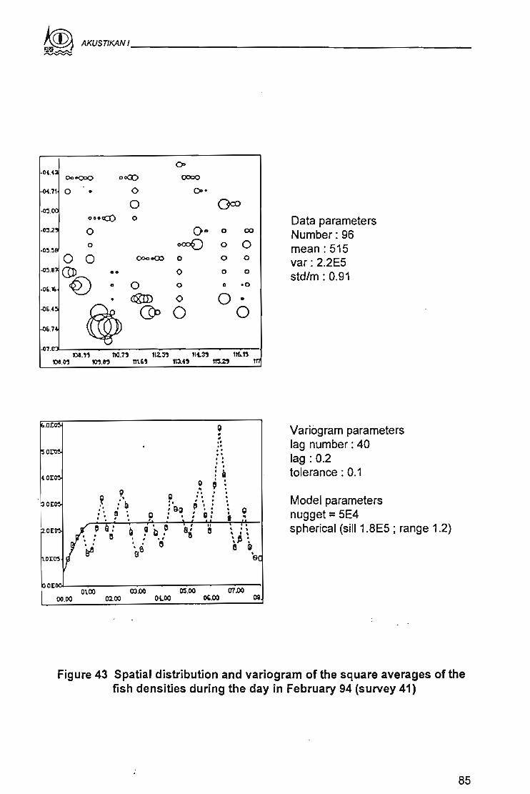
~ AKUSTIKANI _

~

C>-

OD 0 00

ooe() 0 0


o -0

o 0

o 0

O·a

oo 0

~ 0

C9'O

o

ocCO

oo

o

o ..ceo

ou. OooÇcO

OUI 0 •

~.OC

.~.2~ 0

~E..4·

-0(, .74

g

.,1,1.'Il..

• 1• 1: ~

~ ~ :I, ••" . ,~ <1.: 'I

: D: ~ ~

9,:' b

Il •, .g": Bg. '

"e1, "..,

'J! 1è Q,

Varioqrarn parameterslag number : 40lag: 0.2tolerance : 0.1

Model parametersnugget =5E4spherical (sil! 1.8E5 ; range 1.2)

0\0000.00 02.00

03..00 ~.OO rn..00oœo 0'.00 ca

Figure 43 Spatial distribution and variogram of the square averages of thefish densities during the day in February 94 (survey 41)

85

AKUSTlKANI _

1000E 10s0E 11<J'E 112"E 116"E 118"E

Density (U.I)

o 1000 2000 3000 4000 >

118"E116"E1

114Of:112"E11<J'E1œ"E1000E

·~.O

1 (b)

6"sJU'; ., ".

Figure 44 Interpolation (krigging method) of the fish density in the area ofthe cruise made in October 93 (survey 34)

(a) Day (b) Night

86

~ AKUSTlKANI _

Table 2 Evaluation table

Squares

Region

Relative error

Mean1survey

34 Night

4000

4754

18.20%

515

34 Day>

13,000

7679

13.20%

1083

12,000 120,000

10,110 20,454

15.00% 14.10%

993 2576

The precision of the surveys is satisfactory. Although the inter distance

transect is very large, the statistical homogeneity and spatial regularity of

the data make the estimation possible with such survey design.

The variance values can be slightly underestimated due to the fact that the

samples in the squares are not random.

Maps of the square averages, Le. maps of the long range structure have

been derived by krigging (Fig. 44). The neighbourhood parameters used

are:

• radius of circular neighbourhood : 3 degrees

• maximum and minimum number of samples used : 5

2.4. Conclusions

The synthesis of these observations leads us to the main conclusions that

follow.

Bjologjcal description : it is possible to describe a biological model of the fish

distributions in the Java Sea, at least inside the survey area. This area is

inhabited by three groups of fish :

87

~ AKJJ811KANI _

• a coastal group, Iinked with continental waters, Iimited in the

shallow water area, This group presents high densities, numerous

schools, but Iittle is known about it (Fig. 45a).

• a widely distributed group, observed ail over the survey area (group

2), with very constant characteristics. This group seems more

strictly pelagie than the others, and is visible by day as weil as by

night (Fig. 45b)

• a dense eastern group, the only one with important migrations

during the year and even during the day. This group is suffering the

most important fishing effort from the large purse seiners (Fig. 46)

Evaluation : the sampling methodology has proved that it is usable for

acoustic stock evaluation, with a good· precision, through the use of the large

surveys (Le. February or October). The distribution presents two kinds of

gradients:

• a gradient West-East, during the dry season, with the main

densities at the east.

• a gradient North-South, during the wet season. This gradient may

exist during ail the year, but is not important enough to be observed

when the high eastern densities are present in the area.

The structures of the distribution are of two kinds :

• a smail structure, with a dimension approximately 5 to 20 nautical

miles, all over the area ;

• a larger structure, which representents the gradient on the whole

area.

88

~ AKUSTIKANI _

!Ie~

100'1: 1œaE 11O"E 112"1: 1140E 11SOE 11Boe1 1

.~[)

(a)

~

1> •

~o~

11O"E 112"1: 1140E 11SOE 11Boe

Figure 45 Repartition ail over the year for (a) group 1 and (b) group 2

89

~ AKUSTlKANI _

~$J'...

1000E1

-:(a)

11O"E 112'1: 1140E 11SOE 11aaE

1> •

1000E 1œoE 11O"E 112'1: 1140E 11SOE 11aaE1

·~W

(b) i-

Figure 46 repartition for group 3 (a) in February and (b) in October

90

~ AKUSTIKANI _

'l..~

Considering these structures, the transects west-east covered during the short

surveys sample correctJy the small structures ail over year. They sample also

correctly the west-east gradient when this one is present, Le. in the dry

season. In this season, they sample probably weil the density histogram in the

area. Neither they do not sampie the N-S gradient, nor the histogram in this

period, but if we consider the first aim of the surveys, which was to evaluate

the density of the population exploited by the purse seiners, Le. the group 3,

one may consider that they represent a valuable tool for that evaluation.

Neverthless a test on this conclusion has to be performed before to consider it"'-.,..

as demonstrated.

When considering the large surveys, it has been shown that the expected

precision of the evaluation could be around 15% on the density evaluation.

This low value compared to the relatively small sampling is due to the great

regularity of the structures observed in the area.

From these results of the Workshop, we may define the future works needed.

The first one will be to have a confirmation of the biological models that are

presented in this document, particularly considering more in details the

information available on the fishery and the fishing experiments made during

the acoustic surveys (Fig. 47 and 48). The species proportion could help to

define the biological meaning of the three groups. The measurements of TS

and its interpretation will be made necessary.

One of the key points to be studied is the fish migrations and movements. The

vertical daily migrations would help to discriminate groups 2 and 3, thus to

make easier the stratification.

The area of the survey does not allow one to extrapolate outside of the central

Java Sea. It would be important to have at least an idea on the structures of

the coastal populations, on the south as weil as on· the north. What is

91

~ AKUSTIKANI _~

~ Surfaœ,

1

Group 2

(a)

1"~b8j~ ~~

.-1

1 Surfacer--------~--~~~----- ~----~-~1

~1

Group 2

!1

(b)

Figure 47 Circadian distribution of fish along the West-East transect(October)

(a) Day (b) Night

(During the day, group 3 is too close to the bottom to be observed throught acoustics)

92

~ AKUSTIKANI _

~

1 SufaœI~~--~~1

i

i

Group 2

(a)

.-

I~Surfaœ1

Group 2

1

1

1 (b)1

r----.SeBbed~ ~~

Figure 48 Night annual distribution of fish along the West-East transect

(a) October (b) February

93

~ MU!mKANI_" _

happening on the west is also not described. Some larger surveys ail over the

Java Sea could give valuable information on this point.

The discrimination between the group 2 and the plankton biomass wouId also

help to understand the behaviour of that group present in ail the Java Sea. As

the surveys have been recorded using a very low threshold, a playback with

other threshold adjustements will give a good idea of the group 2. In the same

idea, the plankton patch could be observed through the different mappings

using different thresholds, and maybe to explain the small structure present

everywhere.

The relationship between the structures of the fish distribution and the fishing

strategy is interesting to study

94

AKUSnKANI _

2.S. References

This very short bibliography ineludes both references whieh have been directly

useful for AKUSTIKAN l, and more general works important for aeoustie stucles

in Indonesia

ANONYMOUS, 1984. Report on 1982-83 aeoustie surveys of pelagie fish

resources in Southem part of South China Sea, with special reference to the

waters around Natuna, Anambas, Serasan and Tambelan Island Groups

CIPNEAO lndonesjan Fjsheries Pevelopment project, GCP/INS/056/CAN,

121 p. mult.

ANONYMOUS, 1991. Target strength postprocessing program ESPTS

Bjosonjcs Inc., Seattle, 41p.

ARMSTRONG M., RENARP D., RIVOIRARD J., PETITGAS P., 1992.

Geostatistics for fish surveydata. Centre géostat. Fontainebleau, 91p.

BOELY T., MARTIN L1NTING, PETIT P., POTIER M., NURHAKIM S.,

SUJIANTO, 1987. Estimation of abundance of pelagie fish in the central part

of the Java Sea (Indonesia). ORSTOM - BPPL Jakarta, 108 p. mult.

BOELY T., POTIER M., PETIT P., MARCHAL E. CREMOUX J.L., NURHAKIM

S., 1986. An evaluation of the abundance of pelagie fish around Seram and

Irian Jaya. ORSTOM, Etudes et thèses, 225p

BURCZVNSKI J., 1982. Introduction to the use of sonar systems for

estimating fish biomass. EAO Fjsh, Techn, paper, No. 191 Rev.1, 93p.

PINER N., 1991. Ines Movies, Manuel de l'utilisateur. ORCA Instrumentatjon

Brest, 88p. mult.

95

~ AXUST1KANI _

DURAND J.R., PETIT D., 1995. The Java Sea environment. BIODYNEX,

POTIERM. and NURHAKIM S. ed., pp 15-38

GERLOTTO F., 1993. Méthodologie d'observation et d'évaluation par hydro

acoustique des stocks tropicaux de poissons pélagiques cotiers : impact du

comportement et de la distribution spatiale. Thèse Doctorat Brest, 300p. mult.

GERLOTTO F., 1993. Rapport de mission à Jakarta (14/11-4/12/93).

Protocole de traitement et d'analyse des données acoustiques de la Mer de

Java. PELFISH Report Jakarta, 31 p.

JOHANNESSON K.A., MITSON R.B., 1993. Fisheries Acoustics. A practical

manual for aquatic biomass estimation. FAO Fish. Techn, paper, 240, 249 p.

MASSE J. CADIOU Y., 1995. Oedipe, guide de l'utilisateur. Organisation et

Exploitation des Données issues d'Ines Movies et des Pêches

Expérimentales. Version 5. IFREMER Nantes, 59p. mult.

PETITGAS P., 1991. Contributions géostatistiques à la biologie des pêches

maritimes. Thèse Doctorat ENS Mines de paris Paris, 220P. mult.

PETITGAS P., PRAMPART A., 1993. EVA, Logiciel de géostatistique pour

IBM-PC effectuant l'analyse structurale et les calculs de variances

d'estimation de quantités totales pour des données géographiquement

corrélées. International Council for the Exploration of the Sea (ICES)

Copenhague, D 65, 55p miméo.

POTIER M., NURHAKIM S., 1995. BIODYNEX : Biology, Dynamics and

Exploitation of Pelagic fish in the Java Sea. ORSrOM / MRD Jakarta, 282p.

SIMMONDS E J., W1LLlAMSON N.J., GERLOTTO F. AGLEN A., 1992.

Acoustic survey design and analysis procedures ; A comprehensive review of

96

AKUSTIKANI _

current practice. InternatiQnal CQuncil fQr the ExplQratiQn Qf the Sea (lCES)

Copenhaçue, 187, 131 p.

SORIA M., 1994. Strucure et stabilité des bancs et agrégatiQns de poissons

pélagiques cotiers tropicaux : Appllcatlon halieutique. Thèse DQctorat

Rennes,l Rennes, 284p.

VENEMA S.C., 1976. Report Qf the operations and results Qf the UNDP/FAO

Vessel LEMURU in lndonesian Waters. Fisheries DevelQpment and

Management project. INSa2/064 Jakarta, 10 parts. mult.

97

l1î)' AKUSnKANI _

~

3. ROUND TABLE

INTRODUCTION

At the end of the AKUSTIKAN 1Workshop, a round table on fishery acoustics

took place in SubBPPL Ancol meeting room, on December 12, 1994. The main

topic of this round table was to discuss the results obtained in the workshop with

people which where not directly involved in PELFISH and/or acoustics. Beyond it

was the opportunity to enlarge the discussion upon the uses and the needs for

acoustics fishery science in Indonesia.

The Round Table participants (ANNEX 2) and Workshop objectives were

presented by J.R. DURAND, Director of the PELFISH Project.

J.R. DURAND:

Thank you for being in this round table. Sorne of you were present last March

at the first PELFISH seminar on biology, dynamics and exploitation :

BIODYNEX. The publication regarding this event will be sent to you before

mid 95. The objective of the Pelfish Project is to draw a general frame for the

management of the Java Sea small pelagic resources. Acoustic sciences offer

an invaluable tool to achieve this goal. This first workshop AKUSTIKAN 1

allowed sorne processing, mapping and reporting of the data collected by the

research vessel Bawal Putih 1since the beginning of the Project.

From the synthetical abstract which we are able to draw now, we can initiate a

discussion on the workshop results and the future of fishery acoustics in

Indonesia as weil as issue sorne recommendations for the next cruises and

the next workshop AKUSTIKAN" which is planned for January 1996.

D. PETIT, in charge of the Pelfish acoustic studies, will present the means

used to collect the data, then, F. GERLOnO will give you sorne of the results

achieved by the workshop team.

98

~ AKUSnKANI _

O. PETIT

The data processed during the workshop AKUSTIKAN 1concem a number of

parameters such as the fish density, its location, species and environmental

conditions. They have been collected during six cruises on transects from

Semarang to Pulau-Pulau Kecil of Matasiri and two surveys covering the

deepest area - more than 50 m - of the Java Sea. The cruises were carried

out by using the Research Vessel Bawal Putih 1. To cover the whole Java

Sea, we would have needed cruises lasting 1 to 2 months aboard a vesser of

10 knots speed. The Bawal Putih 1 is capable only 12 days sailing with an

average speed of 6 knots. This is why we had to adopt much more simple

surveys. The equipment used is presented in Figure 2.

F. GERLOnO

Since the transects did not cover the whole Java Sea, the area studied is

shown in Figure 1.

The sets of data we used during the workshop were related to :

• Salinity : which varies according to the seasons

• TS measurements : The values of TS measurements vary

according to the length of the fish, the altemate day and night, and

seasons. We can observe bigger fish at night.

• Schools . : The schools have a very original behaviour in the

Java Sea which affects the stock. We can notice on Figure 16 that

school concentrations in the east part of the Java Sea are of

medium density while in the west they are of a higher density.

• Oensity : The density data are of the most importance and

lead to interesting questions such as :

- Is the low density observed in February proving a migratory

behavior?

99

~ AKlJSTIKAN, _

• Why in October the density is higher in the eastern part than in

the western part of the transect ?

• Why day values are half of the night values?

Particularly, the topic was to know if the spaced surveys (or transects only),

were satisfactory to describe the phenomena, evaluate the density and its

location. The use of geostatistics during the workshop showed us that on the

whole of the Java Sea, the density is structured at very small scale (sorne

miles); but a large scale structure is superimposed on this later. It is the large

scale structure that interest us. The survey strategy with large transects,

chosen by the Project, is weil adapted to the structure pattern of the Java Sea.

Using geostatistics, the large surveys allow us to evaluate the density with an

accuracy of about 20%, that is very satisfactory.

The conclusions of the workshop, on the six cruises studied, agree with the

biological conclusions given in the last BIODYNEX seminar. We can build a

model with three zones as shown on Figure 30 :

• zone A, with a coastal population

• zone B, with a neritic population

• zone C, with an oceanic population,

and it appears that these three zones are related to the fisheries. This is a

good match with the biological zonations.

100

~ AJ<USTl/WI' _

DISCUSSION

ln order to give some clarification to the questionlanswer process, we have tried

to give a more logical form to the discussion. So the order has been changed

and we put together related topics without changing the original material.

Methodology

CHOLIK : Why did you select only 6 surveys for your workshop?

PETIT : Cleaning the raw data then process them, takes much

longer time than the workshop itself. The workshop validates

only some data as a beginning. One of the conclusions of

this week is that we need more people to validate the data.

We hope that this workshop will give place to work proposais

with Bogor Agriculture University (West Java) and Sam

Ratulangi University (North Sulawesi)

DURAND : The Java Sea is probably the only place in the world where

so much information has been gathered and where the

information is so original. Yet Indonesian acousticians are

too few.

CHOLIK : Would it be better to process data just after each cruise?

DURAND : The principle is a good one but practically it is very difficult.

PETIT : At the beginning we had only three weeks between each

survey. It is not enough time to start any work on data.

DE VISSCHER : It is not unusual to analyse data later, Acoustic planning

depends on boat availability as weil as computer availability.

ln the consolidation phase it is important to collect data.

DURAND : We face a lack of time and people. We also need more

equipment and more coordination.

101

~ AKUSTIKANI _

AMIN

PETIT

GERLOnO

NURZALI

GERLOnO

DURAND

Specifie results

FATUCHRI

WIDODO

NURZALI

: Why did you use INES-MOVIES in place of the Biosonics

software?

: With INES-MOVIES you can store numerical data. It also

provides outputs echograms in color. Now Indonesia has a

very important database.

: The most interesting phenornenon of the Java Sea is that

its structures are regular. Mapping the information would

take a long time but it should not be difficult to obtain

indexes.

: WouId this allow remote sensing management?

: Satellites can monitor environmental structure and several

works of this type have been financed by the EU. But they

still present sorne Iimits. Toois are not yet very usable and

they have not yet overcome the problem of clouds.

: We need more data on primary production.

: Pelfish should fumish information on the movements and

size of the biomass but also on its magnitude. We should

have data not only on salinity but also on food organisms

like plankton . An ecological management plan is an easier

path for recommendation.

: A research on food organisms would be time consuming.

Moreover it ls not our primary task. Thére is a number of

weaknesses in using indirect approaches for biomass

estimation.

: What does the difference in depth of the schools locations

between day and night mean ? Does it vary according to the

species?

102

t@1 AKUSnKANI _

~.,.y'...

GERLOTTO : One of the Iimits of echo integration is that the system can

not integrate down the surface ( from 0 to 4m ) and near the

bottom of the sea. This makes it difficult for us to describe

the change of behaviour between day and night. We

assume that at day time the fish stay very near the bottom of

the sea.

PETIT : The density peaks take place twice a day, around 5 AM

then between 5 and 6 PM.

POTIER : Even from the biological point of view it is difficult to be

sure that the fish stay at the bottom of the sea : due to

currents, the seines never go straight the bottom.

GERLOTTO : The fishery tactics with light affects the relation between

the seine parameters and the natural behaviour of the fish.

PRIONO : How can we use the information we have on spawning

seasons to optimize the management?

SADHOTOMO : We recognized two spawning seasons : one from January

to April, the other one from August to October. Which means

two recruitments periods, a major one from May to August

and a minor one from December to January dUling the

north west monsoon.

DURAND : Can we observe spawning concentrations?

POTIER : It is difficult to observe as 80% of ail fish caught are

immature ones, fish that have not yet spawned.

GERLOnO : To answer the question we need more information about

the north of the Java Sea but not about the west.

NURZALI : Is the Hardenberg theory proven true or not?

DURAND : Up to now we haven't proven any connection between the

Java 'Sea and the South China Sea. But we plan to start

genetic studies on some common species of the regions.

103

~ AKUSTIKANI _

,..."" :;J\;'\.

DURAND

POTIER

DURAND

NURZALI

DURAND

CHOLIK

DURAND

: Could it be there a continuation of the nereüc system?

: Salinity on the west is low.

: Are there fisheries on the west part of the Java Sea?

: Not very developed.

: Maybe because there are not enough fish.

: This is something the project Pelfish needs to prove.

: Do we? Is it pelagic? We need your recommendation to

investigate this topic.

DE VISSCHER : If acoustic is needed for the future we need a proposai

from indonesian authorities. It should be a long-term

proposaI.

Management

DE VISSCHER : How can acoustics studies contribute to management on

the long term?

NURZALI

PRIONO

DURAND

NURZALI

: What is the use of more Pelfish cruises for the resource

management?

: ln your conclusions will you take into account economical

analysis, depletion of the stock, critical situation of other

stocks such as the "Iemuru" in Bali?

: We plan to publish three books, one on Biology, Dynamics

and Exploitations (BIODYNEX) one on Acoustics, and one

on Social Sciences and Technologicallnriovation.

: Is there not already enough data for management

planning?

104

PASARIBU

~ MUSTIKANI "'-_

DURAND : We have a global knowledge which is now backed up by

the acoustic results. We can already start working on

management.

PRIONO : 1 have impression that my department is left behind with

the information coming from the Project. We need

information specially on stock assessment !

POTIER : And specially because your own statistics are incomplete.

PRIONO : We have no complete statistics yet on stock assessment

but we will have logbooks on data.

DURAND : The quality of governmental statistics is variable among

fisheries and landing places. For Central Java, the region

that we are concerned with, we have no major difficulties.

DURAND : The collaboration between Pelfish and the DGF is a

priority. We plan the arrivai of an expert in management who

will be working with the DGF and weil trained scientists.

De VISSCHER : This is the goal of the consolidation phase which has been

signed last week in Brussels. It is too early to know if the EU

will finance another Project. However translating the

management plan into practice will be a higher priority than

further research.

Perspectives

: What is the aim of the Project? It just gives a general view

of the pelagie fishes in the Java Sea, don't you have made

enough transects already ?

DE VISSCHER : Do we need more campaigns ? Several or just one?

GERLOnO : We are talking in the frame of 18 months consolidation

phase.

105

~ AKUSTIKANI _

POTIER

DURAND

: We need several other cruises to establish comparisons

and define the importance of environment between the

years.

: From Figure 30, we can see where should be the

complementary cruises during the consolidation phase: in

Makassar Strait (north of Area C), in South Kalimantan

waters (north of Area B), and in West Java Sea waters (west

of Area B). We are also planning to have a joint program

with Bogor Agriculture University in order to better survey

Area A.

POTIER

DURAND

DE VISSCHER : What is the priority of PELFISH in the Java Sea ?

: It seems that there are more pelagies to catch on the

eastern part than on the western part of the Java sea.

: But interest can change priorities. And we should get on

the western part to realize if this region is of interest or not.

DE VISSCHER : What is the cruise plan for the consolidation phase?

DURAND

GERLOTTO

: The next transects will be different from the previous ones,

they will be outside the areas already checked :

1. Lumu-Lumu in Makassar Strait.

2. We expect a program with Bogor Agriculture University on

North Java coastal waters.

3. West Java. We recommend two cruises of 10 days

respectively.

4. We will collect landings data in South Kalimantan.

: The Research Vessel Bawal Putih l, is not useful in shallow

waters less than 25m depth. The fish goes away.

106

~ AKUSTIKANI _

DURAND

AMIN

POTIER

GERLOTTO

CHOLIK

DURAND

: It would be useful to organize a cruise with two vessels.

: Maybe you should organize smaller cruises at other

seasons, specially in May-June.

: Fishermen say that there are no fish in May and June in

the Java Sea

: The strategy is not to make a lot of transects : the Java

Sea structures are regular enough to not shorten the

distance.

: Can PELFISH Project provide training. ICLARM invited

sorne CRIFI experts already but we need more training

programs.

: We do have programs for the PELFISH national scientists.

You will just acquire a new research vessel, the Baruna Jaya

IV. This vessel should be dedicated to acoustic surveys and

develop the future of acoustics in Indonesia. This boat will

have a lot of equipment, as weil acoustic equipment as

fishing devices for sampling. The prospection of the EEZ

needs to be planned carefully with trained people.

107

4.

AKUSTIKANI _

ANNEXES

4.1. Annex 1 : Workshop announcement

WORKSHOPANNOUNCEMENT

The Java Sea Pelagie Fishery Assessment Project ALAlINS/87/17, a project

mainly financed by the European Union, is carried out by ORSTOM France

and BPPL Indonesia.

Since 1991, it has conducted a research program aimed to the knowledge

and management of the Java Sea Pelagie Fisheries. Many stock evaluation

cruises have been undertaken using the acoustic echo integration method.

The exploitation of the collected data has already started out and the Project

has decided to set up a week workshop on these observations.

"AKUSTIKAN"

The theme of the workshop is :

The Stratification of The Data,

a subject which is of major importance for the spatial and temporal

quantitative evaluation. Possibly, a second theme of study could be selected

according to the general interest of participants.

108

~ AKUSTlKANI _

This workshop will be of primary interest to scientists specialized in echo

integration and who wish to emphasize their experience through the Pelfish

data. Apart from Pelfish scientists we can already count on the participation

of Doctors F. GERLOTTO and P. PETITGAS, weil known as ORSTOM

specialists. Sorne young scientists or students could also participate to the

event but in order to maximize the efficiency of the work the total number will

be limited to sixteen participants.

The 16 participants will be divided in four groups, every one using a computer

with the following softwares: OEDIPE, EVA, EXCEL, SURFER ESPTS,

LOTUS and STATGRAPHICS.

The data available for this workshop have been collected during 4 echo

integration cruises (with a DUAL BEAM 120 kHz BIOSONICS echo sounder).

Two of these cruises concern the three quarters of the Java Sea surface

during the two opposite seasons; a third one concerns two transects from

Java up to the south of the China Sea. During this one, observations were

made on a median transect throughout the Java Sea and at small spatial

scale, by day and by night in three different sectors of the Java Sea. Data

include also environmental measurements (temperature and salinity by

station) and results of identification catches (pelagic and bottom trawls, or

purse seiners sampling).

The corresponding files contain :

• the temperature/salinity measurements by meter at stations,

• the inventory of species (weight) by trawl catch,

• the relative abundance of tish (total or by layer) by mile,

• the number of echo-reverberating elementary samples (total or by layer),

• the number of elementary samples insonitied,

• the spatial and bathymetric location of aggregations and their relative

reverberation,

• the TS in situ measurements by station (average value and distribution).

109

~ AKUSnKANI _~..::::n..

This workshop will take place at

BPPLANCOLJAKARTA

FROM DECEMBER 5TH TO 12TH, 1994

The sessions will start at 9.00 A.M. every day. The event will close on the

12th with :

• In the morning, a presentation about the conclusions of the common

investigations and some recommendations for the prolongation of

the Project's research.

• In the aftemoon, starting at 2.00 P.M. a "round table" including

personalities from outside of the Project in order to mention the

problems conceming the development of echo integration in terms of

equipment, users and organisation in Indonesia.

110

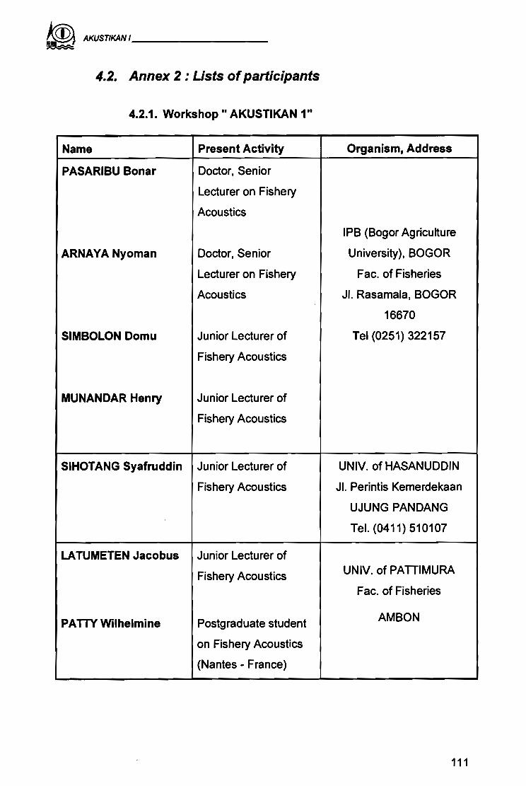
~ AKUSTIKANI _

4.2. Annex 2 : Lists ofparticipants

4.2.1. Workshop" AKUSTIKAN 1"

Name Present Activity Organism, Address

PASARIBU Bonar Doctor, Senior

Lecturer on Fishery

Acoustics

IPB (Bogor Agriculture

ARNAYA Nyoman Doctor, Senior University), BOGOR

Lecturer on Fishery Fac. of Fisheries

Acoustics JI. Rasamala, BOGOR

16670

SIMBOLON Domu Junior Lecturer of Tel (0251) 322157

Fishery Acoustics

MUNANDAR Henry Junior Lecturer of

Fishery Acoustics

SIHOTANG Syafruddin Junior Lecturer of UNIV. of HASANUDDIN

Fishery Acoustics JI. Perintis Kemerdekaan

UJUNG PANDANG

Tel. (0411) 510107

LATUMETEN Jacobus Junior Lecturer of

Fishery Acoustics UNIV. of PATIIMURA

Fac. of Fisheries

PATTY Wilhelmine Postgraduate student AMBON

on Fishery Acoustlcs

(Nantes - France)

111

~ AKUSTIKANI:.... _

...... . ..".

Organism, Address< .Ham8 .: Present Activity

MUBARAK Junior Lecturer of UNIV. of RIAU

Fishery Acoustics Fac. of Fisheries

Kampus Bina Widya Km.

12.5

PEKAN BARU 28293

LlMBONG Daniel Doctor, Lecturer on UNIV. of SAM RATULANGI

Fishery Acoustics Dept. of Marine Sc.

Education

MANADO

Tel. (0431)62486

NAINGGOLAN Chandra Doctor, Lecturer on STP (College of Fisheries)

Fishery Acoustics P.O. Box 7239/JKPSM

JI. AUP Pasar Minggu

JAKARTA

Tel. (021) 7805030

GERLOTTO François Doctor, Fishery ORSTOM MONTPELLIER

Acoustician BP 5045

34032 MONTPELLIER Cx 1

PETITGAS Pierre Doctor, Geostatistician Tel (001.33) 67 67 74

PETIT Didier Fishery Acoustican

COTEL Pascal Engineer Acoustician ORSTOM PELFISH

"II. Pasir Putih 1 Ancol Timur

LUONG Nicolas Engineer Jakarta 14430

Tel. (021) 68 9897NUGROHO Duto Junior, Acoustics

Biology

112

AKUSnKANI _

4.2.2. Round table

Institution representatives and invited scientists

Mr. Vincent DE VISSCHER

Dr. Fuad CHOLIK

Dr. Fatuchri SUKADI

Dr. Nurzali NAAMIN

Dr. 1Gde SEDANA MERTA

Mr. Edy MULYADI AMIN

Dr. Bambang EDI PRIONO

Mr. Gomal TAMPUBOLON

ORSTOM Scientists

Dr. François GERLOnO

Dr. Pierre PETITGAS

Participants to the workshop

Dr. Bonar PASARIBU

Dr. Nyoman ARNAYA

Mr. Domu SIMBOLON

Mr. Henry MUNANDAR

Mr. Syafruddin SIHOTANG

Mr. Jacobus LATUMETEN

Mrs. Wilhelmine PAnvMr. MUBARAK

Dr. Daniel LlMBONG

Dr. Chandra NAINGGOLAN

Representation of the E.U.

Director, CRIFI

Director, RIFF

Director RIMF

Senior Scientist, RIMF

Senior Scientist, RIMF

Living Resource Management, DGF

Living Resource Management, DGF

Expert in fishery acoustics who animated the

workshop

Expert in Geostatistics

Senior Lecturer on Fishery Acoustics

Senior Lecturer of Fishery Acoustics

Junior Lecturer of Fishery Acoustics




Postgraduate Student on Fishery Acoustics


Lecturer on Fishery Acoustics

Lecturer on Fishery Acoustics

113

~ AKUSnKANI _

ThePelfish Scientists.. .

Dr. Jean René DURAND

Dr. Johanes WIDODO

Dr. Didier PETIT

Mr. Michel POTIER

Mr. Bambang SADHOTOMO

Dr. Subhat NURHAKIM

Mr. Duto NUGROHO

Mr. Nicolas LUONG

Mr. Pascal COTEL

Director

Co-Director

Bio-Acoustician

Biologist

Biologist

Biologist

Junior Acoustics Biology

Agronomist Engineer

Acoustician Engineer

114

~ AKUSTIKANI _

~

4.3. Annex 3 : Cruises, main characteristics

Abbrevjatjons used :

Transitfrom Semarang to ...

f and from ... to Semarang

Meteorology

Moon

Log, radar, GPS

Navigation

Engines

Environnement

Sampling

Transect SMG ->

Gridding, transect

Siope

PS-PS

Attractions

TS while anchored

TS during transect

Calibration

Various

G = goOO ; M = medium (force2-3 Sea) ; 8 = bad (force 3-5

Sea)

O=new moon ; 1=firstquarter; 2=fullmoon ; 3 =Iastquarter

G = goOO functioning ; M = average functioning; N = absent

or malfunction

G = precise positioning ; M = average or occasional

positioning, N = estimated positioning withouteJectronic

equipment

G = goOO (speedaround 7 knots); M = medium ( == 6 knots)

; B = bad (== 5 knots or lesswith occasional stops)

y = operational ; N = not operational

y = samples realized : N = no samples realized

Matasiri (Mat)

Masalembo (Mao)

Bawean (Baw)

Tambelan (Tam)

NorthSemarang (Nam)

NO= routes repeated during the day and the night : N =

only one routeduring the night : A = only one routeduring

the day and the night

y = route along the slopeof the continental shelf

o = random routeby night from seinerto seiner

Number of Iightattraction realized

y = TS measurement made at the anchorage on fish in cage

y = TS measurement made on the way

y = Equipement calibration

AIE = routewith illumination phase

Maco = coastal routearound Matasiri

PPS= positioning of purseseiner

RU = Attraction under rumpon

BPper = routearound Bawal Putih whileattracting by Iight

115

~ AKUSTIKANI _

led'<*

M

4

G

4

G

o

Mar.Month ...

·Yëar ..

1

Meteorology

Moon

VESSEL

Log M M N M M M M

Radar M M N N G G G

GPS N N N G G G G

Navigation M M M G G G G

Englnes G GlM G M G G MlB

ENVIRONMENT

Thennosallno N y Y Y Y Y Y

Profiles N N Y Y Y Y Y

Quantameter N N N N N N Y

SAMPLING

Pelagie trawI . N N N N 1···· N N> ·N·'·

Bottom trawl N N N N .....y y y

PurseSelner y y y y y y N

ECHO INTEGRATION

Transit SMG -> MatIMat MatIMat MatIMat MatIMat MaolMao MaolMat MatIMat

Grlddlng 2*ND ND ND 2*A A A

Transec:t ND N

Siope A

PS-PS 0

Attraction 3 2 2

TS

Anchored y Y

On the W8'1 y Y Y Y .y Y Y

1 CALIBRATION y y y y y

1 VARIOUS AlE Maco PPS PPS PPS

116

~ AKUSTlKANI _

Vear

Month Apr. 1 May 1 Jun. 1 Oct. 1 Nov. 1 Dec;Feb.<i>/Apr.

1

Meteorology

Moon

B

o

VESSEL

Log M M M G G G G G

Radar G G G G G G G G

GPS G G G G G GIN G G

Navigation G G G G G GIN G G

Engl".. M M B G G M B G

ENVIRONMENT

Thennosallno y y y y y N Y Y

Profiles y y y y y y y y

Quantameter y y y y y y y y

.'. <. ...SAMPLING <: ..... .. ........:...........Pelagie trawI ... Y·" .N Y Y 1" Y Y 'y> 1 s:'.">' . .

Bottom trawI Y N N Y Y. y .... y ..... y

Pu,... Seiner . y y N Y Y Y Y. ..... N'

ECHO INTEGRATION

Transit SMG -> TamITam BawlBaw BawlBaw MatIMat MatIMat MatIMat MatIMat NsmINs

Grtddlng ND N A N NID A

Transec:t NID NID NIDSiope N N Y Y

PS-PS 0 0

Attraction 1 8 1 1 7 5

TS

Anchcnd.

OntheWl'/ y y y y y y y y

1 CALIBRATION

1VARIOUS PPS

1 1

RU 1 BPper 1

1 1

PPS 1 BPperlRU 1

y

RU PPS

y

117

AGENCY FOR AGRICULTURAL RESEARCH AND DEVELOPMENTRESEARCH INSTITUTE FOR MARINE FISHERIES

JAVA SEA PELAGIe FISHERYASSESSMENT PROJECT

( ALAlINS/87/17 )

Jaian Pasu Putih 1. Ancol Timur. JAKARTA 14430, lndonesia. Tel./Fax. (6221 )-689897

-

Dear Reader,

Jakarta 1 August 1995

Concerning the report on the Workshop "AKUSTlKAN 1", Scientific and TechnicalDocument No 21, June 1995, the Table 2, page 87, includes an inversion ofcolumn. Ithas to be read as joined. We are sorry for this error...

The Editors

ERRATUM: The Table 2.page 87.has to be changed as folJow:

Table 2: Evaluation table

SurYey:,}~ NÎgfitm gtf~;Dayk% fff.41Night ; 41 Day

•..._~

SquaréS' 120.000 12.000 13.000 4.000"". ;:.Î','"

;'J~-". ' ;~?:.' '".~i6it;:F\· 20.454 10.1 10 7679 4754

.""';'.:.-". ·-.;·-:"f~~ .;;.:,:-~.:

.~~'.' .;.:::.

Rel~'. ·::.,::t~:·~·: ~.~.:

14.10% 15.00% 13.20% 18.20%error"" ,.,.

MeanlSiJrVèY·': 2576 993 1083 515

java sea pelagic fishery assessment...

Documents