Java Generics are Turing Complete

Radu GrigoreUniversity of Kent, United Kingdom

AbstractThis paper describes a reduction from the halting problem of Turingmachines to subtype checking in Java. It follows that subtypechecking in Java is undecidable, which answers a question posed byKennedy and Pierce in 2007. It also follows that Java’s type checkercan recognize any recursive language, which improves a result ofGil and Levy from 2016. The latter point is illustrated by a parsergenerator for fluent interfaces.

Categories and Subject Descriptors D.3.3 [Language Constructsand Features]

Keywords Java, subtype checking, decidability, fluent interface,parser generator, Turing machine

1. IntroductionIs Java type checking decidable? This is an interesting theoreticalquestion, but it is also of interest to compiler developers (Breslav2013). Since Java’s type system is cumbersome for formal reasoning,several approximating type systems have been studied. Two of thesetype systems are known to be undecidable: (Kennedy and Pierce2007) and (Wehr and Thiemann 2009). Alas, neither of these is asubset of Java’s type system: the reduction of (Kennedy and Pierce2007) uses multiple instantiation inheritance, which is forbiddenin Java; the reduction of (Wehr and Thiemann 2009) uses boundedexistential types in a way that goes beyond what Java wildcards canexpress. So, neither result carries over to Java.

Not knowing a decidability proof was enough to spur interestinto decidable fragments. In (Kennedy and Pierce 2007), certain‘recursive–expansive’ patterns in the inheritance are forbidden;this solution was adopted in Scala, whose typechecking remainsundecidable for other reasons. In (Tate et al. 2011), some restrictionson the use of ‘? super’ are imposed. In (Greenman et al. 2014),one distinguishes between classes and ‘shapes’. Here, we shall provethat Java’s type system is indeed undecidable, which justifies furtherthese existing studies.

In a separate line of work, (Gil and Levy 2016) show that Java’stype system can recognize deterministic context free languages, thusgiving the first nontrivial lower bound directly applicable to Java’stype system. Our main result immediately implies that Java’s typesystem can recognize any recursive language. In addition, we shallshow that Java’s type system can recognize context free language inpolynomial time. More precisely, the two results are the following:

Theorem 1. It is undecidable whether t <: t′ according to a givenclass table.

Theorem 2. Given is a context free grammar G that describes alanguage L ⊆ Σ∗ over an alphabet Σ of method names. We canconstruct Java class definitions, a type T , and expressions Start ,Stop such that the code

T ` = Start .f (1)().f (2)() . . . f (m)().Stop

type checks if and only if f (1)f (2) . . . f (m) ∈ L. Moreover, the classdefinitions have size polynomial in the size of G, and the Java codecan be type-checked in time polynomial in the size of G.

Theorem 1 is proved by a reduction from the halting problemof Turing machines to subtype checking in Java (Section 5). Theproof is preceded by an informal introduction to Java wildcards(Section 2) and by some formal preliminaries (Sections 3 and 4).It is followed by Theorem 2, which is an application to generatingparsers for fluent interfaces (Section 6). The parser generator makesuse of a compiler from a simple imperative language into Java types;this compiler is described next (Section 7). Before we conclude, wereflect on the implications of Theorems 1 and 2 (Section 8).

2. Background: Java WildcardsThis section introduces Java generics, wildcards, and their bounds,by example. The presentation is necessarily incomplete. For thedefinitive reference, see (Gosling et al. 2015).

Java generics are used, for example, to implement lists. Whenimplementing the list, its elements are given a generic type. Whenusing the list, the type of its elements is fixed. The interactionbetween generics and subtyping is not trivial. List〈Number〉 isnot a subtype of List〈Integer〉: if it were then we could extractintegers from a list of numbers; nor is List〈Integer〉 is a subtypeof List〈Number〉: if it were then we could insert numbers in a listof integers.

Intuitively, there is a difference between extracting and insertingdata. For example, suppose we want to implement a functionfirstNum that extracts the first number in a list. The implementationshould work for both List〈Integer〉 and List〈Number〉. Wecould use bounded generics

<x extends Number> Number firstNum(List<x> xs){ return xs.get(0); }

or bounded wildcards

Number firstNum(List<? extends Number> xs){ return xs.get(0); }

Both variants bound the elements to be subtypes of Number. Nowlet us consider the converse situation, in which we want to insertan integer into the list. In this case, Java lets us use only the variantwith wildcards:

void addOne(List<? super Integer> xs){ xs.add(1); }

arX

iv:1

605.

0527

4v2

[cs

.PL

] 7

Nov

201

6

As with firstNum, the method addOne can be used with both ofList〈Integer〉 and List〈Number〉.

Now let us consider the call to firstNum, for a list of integers.For the bounded generics version, the call is

this.〈Integer〉firstNum(xs) or firstNum(xs)

The latter is a simplified version, made possible by type inferenceand syntactic sugar. So, let us focus on the former. In it, we setthe type variable x to Integer, thus selecting which version of thegeneric method firstNum we are using. On the other hand, for thebounded wildcard version, the call is

this.firstNum(xs) or firstNum(xs)

This code looks similar to the one for bounded generics, but ittype checks for a different reason: List〈Integer〉 is considereda subtype of List〈? extends Number〉, because Integer is asubtype of Number.

Also, if B is a subtype of A, then List〈? extends B〉 is a sub-type of List〈? extends A〉, and List〈? super A〉 is a subtypeof List〈? super B〉. Finally, List〈?〉 is a supertype of all lists.

Bounded wildcards are used liberally in the implementation ofJava’s standard library. For a more interesting example, consider thefollowing method from java.util.Collections:

static <T> int binarySearch(List<? extends Comparable<? super T>> list,T key) { /* ...*/ }

‘To search for a key of type T in a list, we must have a list whoseelements are comparable to T.’ To express this constraint, we needboth ‘? extends’ and ‘? super’

Java’s mechanism for deciding whether List〈α〉 is a subtype ofList〈β〉 is known as use-site variance because it involves gettinga hint from inside α and β: Do they mention ‘? super’ or ‘?extends’? The alternative, declaration-site variance, is to takethe hint from the declaration of List, where the generic typecan be annotated as being covariant, invariant, or contravariant.We can simulate declaration site variance by use site variance asfollows: if the declaration of L annotates type T to be covariant,then we erase the annotation and replace all uses L〈. . . , T, . . .〉by L〈. . . , ? extends T, . . .〉; for contravariant annotations, weproceed similarly, but using ‘? super’ instead of ‘? extends’.In what follows, we only need the contravariant case, so it is theonly one we formalize.

3. PreliminariesWe formalize a fragment of Java’s type system, following (Kennedyand Pierce 2007). Types are defined inductively: if x is a typevariable, then x is a type; if C is a class of arity m ≥ 0 andt1, . . . , tm are types, then Ct1 . . . tm is a type. Given a class C, wewrite arity(C) for its arity; given a type t, we write vars(t) for thetype variables occurring in t. A substitution σ is a mapping froma finite set dom(σ) of type variables to types; we write tσ for theresult of applying σ to t. A class table is a set of inheritance rulesof the form

Cx1 . . . xm <:: Dt1 . . . tn

such that vars(tj) ∈ {x1, . . . , xm} for j ∈ {1, . . . , n}, wherem = arity(C) and n = arity(D). A class table defines a binaryrelation <:: between types: if tL <:: tR is an inheritance rule, thentLσ <:: tRσ for all substitutions σ. Note that we slightly abusethe notation <::, using it both as a binary relation on types and asa syntactic separator in inheritance rules. When <:: is used as arelation, we denote by <::∗ its reflexive transitive closure. (Notealso that dropping the symbols ‘<,>’ that Java uses is unambiguous,as long as arities are known.)

Java forbids multiple instantiation inheritance: that is, in Java,if t <::∗ Ct1 . . . tm and t <::∗ Ct′1 . . . t

′m, then ti = t′i for

1 ≤ i ≤ m. In particular, if Cx1 . . . xm <::∗ Ct1 . . . tm, thenxi = ti for 1 ≤ i ≤ m; that is, the class table is acyclic.

The subtyping relation <: is defined inductively by the rule

At1 . . . tm <::∗ Ct′1 . . . t′n t′′1 <: t′1 . . . t′′n <: t′n

At1 . . . tm <: Ct′′1 . . . t′′n

(1)

If t <: t′, we say that t is a subtype of t′, and t′ is a supertypeof t. In rule (1), types t′′∗ occur in the supertype of the goal but inthe subtype of assumptions. In other words, we consider only thecontravariant case. It is known that Java’s wildcards can encodedeclaration-site contravariance, and that subtyping is decidable inthe absence of contravariance (Kennedy and Pierce 2007).

Theorem 1 is proved by a reduction from the halting problem ofTuring machines. A Turing machine T is a tuple (Q, qI, qH,Σ, δ),where Q is a finite set of states, qI is the initial state, qH is the haltstate, Σ is a finite alphabet, and δ : Q×Σ⊥ → Q×Σ×{L, S,R} isa transition function. We require δ(qH, a) = (qH, a, S) for all a ∈ Σ,and δ(qH,⊥) = (qH, a,S) for some a ∈ Σ. A configuration is atuple (q, α, b, γ) of the current state q ∈ Q, the left part of the tapeα ∈ Σ∗, the current symbol b ∈ Σ⊥, and the right part of the tapeγ ∈ Σ∗. The execution steps of T are the following:

(q, αa, b, γ)→ (q′, α, a, b′γ) for δ(q, b) = (q′, b′, L)

(q, α, b, γ)→ (q′, α, b′, γ) for δ(q, b) = (q′, b′,S)

(q, α, b, cγ)→ (q′, αb′, c, γ) for δ(q, b) = (q′, b′,R)

We also allow for execution steps that go outside the existing tape:

(q, ε, b, γ)→ (q′, ε,⊥, b′γ) for δ(q, b) = (q′, b′, L)

(q, α, b, ε)→ (q′, αb′,⊥, ε) for δ(q, b) = (q′, b′,R)

(Here and throughout, ε stands for the empty string.) A run on inputtape αI is a sequence of execution steps starting from configuration(qI, ε,⊥, αI). If T reaches qH we say that T halts on αI.Theorem 3 (Turing 1936). It is undecidable whether a Turingmachine T halts on input αI.

4. Subtyping MachinesThe fragment of Java’s type system defined in the previous sectiondoes not seem to share much with Turing machines. To clarify theconnection, let us define a third formalism: subtyping machines. Theplan is to see how subtyping machines correspond to a fragment ofa fragment of Java’s type system, and at the same time can simulateTuring machines. So far, we saw a fragment of Java’s type systemthat included generic classes of arbitrary arity. Subtyping machinescan only handle the case in which all classes have arity 1, apart fromone distinguished class Z which has arity 0. The configuration of asubtyping machine is a subtyping query

C1C2 . . . CmZ <: D1D2 . . . DnZ

For reasons that will become clear later (Example 5), we introducetwo alternative notations for the same configuration as above:

ZCmCm−1 . . . C1 J D1D2 . . . DnZ

= ZDnDn−1 . . . D1 I C1C2 . . . CmZ

Since we restrict our attention to arity ≤ 1, there are two waysin which proof rule (1) can be applied:

C1 . . . CmZ <::∗ Z

C1 . . . CmZ <: Z

C1 . . . CmZ <::∗ D1E2 . . . EpZ D2 . . . DnZ <: E2 . . . EpZ

C1 . . . CmZ <: D1 . . . DnZ

Correspondingly, we define two types of execution steps · · forthe subtyping machine:

(ZCm . . . C1 J Z) •

if C1 . . . CmZ <::∗ Z, and

(ZCm . . . C1 J D1 . . . DnZ) (ZEp . . . E2 I D2 . . . DnZ)

if C1 . . . CmZ <::∗ D1E2 . . . EpZ. The special configuration • iscalled the halting configuration.

Recall that <::∗ is the reflexive transitive closure of a relationdefined by the class table. Thus, in particular, if the class tablecontains the inheritance rule

C1x <:: D1E2E3 . . . Epx

then we can instantiate it with x := C2 . . . CmZ to enable thefollowing execution step:

ZCm . . . C2C1 J D1D2 . . . DnZ

ZCm . . . C2Ep . . . E2 I D2 . . . DnZ(2)

Also, because <::∗ is reflexive, the following execution step isenabled:

ZCm . . . C1N J ND1 . . . DnZ

ZCm . . . C1 I D1 . . . DnZ(3)

The runs of subtyping machines correspond to (partial) proofs.Runs that halt correspond to completed proofs. Runs that getstuck correspond to failed proofs. The subtyping machine may benondeterministic, which corresponds to situations in which one mayapply proof rule (1) in several ways; but, if multiple instantiationinheritance is forbidden, as it is in Java, then the subtyping machineis deterministic. There is nothing deep about subtyping machines:they are introduced simply because the new notation will make itmuch easier to notice certain patterns.

Proposition 4. Consider a subtyping machine described by a givenclass table. We have

C1 . . . CmZ <: D1 . . . DnZ

if and only if there exists a halting run

(ZCm . . . C1 J D1 . . . DnZ) ∗ •Example 5. In preparation for the main reduction, let us look at oneparticular subtyping machine. Consider the following class table:

QLx <:: LNQLLNx QRx <:: LNQRLNx (4)

QLx <:: EQLRNx QRx <:: EQRLNx (5)

Ex <:: QLRNQREEx Ex <:: QRLNQLEEx (6)

and the query QREEZ <: LNLNLNEEZ. Then, the subtypingmachine runs as follows:

ZEEQR J LNLNLNEEZ

2 ZEENLQR J LNLNEEZ by (4)+(2), then (3)

2 ZEENLNLQR J LNEEZ by (4)+(2), then (3)

2 ZEENLNLNLQR J EEZ by (4)+(2), then (3)

ZEENLNLNLNQRL I EZ by (5)+(2)

ZEENLNLNLN J NQLEEZ by (6)+(2)

ZEENLNLNL I QLEEZ by (3)

2 ZEENLNL I QLLNEEZ by (4)+(2), then (3)

2 ZEENL I QLLNLNEEZ by (4)+(2), then (3)

2 ZEE I QLLNLNLNEEZ by (4)+(2), then (3)

interface Z {} interface N<x> {} interface L<x> {}interface Qlr<x> {} interface Qrl<x> {}interface E<x> extends

Qlr<N<?super Qr<?super E<?super E<?super x>>>>>,Qrl<N<?super Ql<?super E<?super E<?super x>>>>> {}

interface Ql<x> extendsL<N<?super Ql<?super L<?super N<?super x>>>>>,E<Qlr<?super N<?super x>>> {}

interface Qr<x> extendsL<N<?super Qr<?super L<?super N<?super x>>>>>,E<Qrl<?super N<?super x>>> {}

class Main {L<?super N<?super L<?super N<?super L<?super N<?superE<?super E<?super Z>>>>>>>>

doit(Qr<? super E<? super E<? super Z>>> v) {return v;}}

Figure 1. Java code for Example 5

Some lines group together two execution steps so that the overallpattern is clearer: we have a head traveling back-and-forth overa tape! The Java code corresponding to (4), (5), (6) appears inFigure 1.

Well-formedness. From (Kennedy and Pierce 2007), we knowthat the subtyping relation is transitive if and only if certain well-formedness conditions hold. Instead of stating these conditions infull generality, let us do it only for our special case, in which aritiesare ≤ 1 and everything is contravariant. Under these conditions,well-formedness requires that, if an inheritance rule has the formAx <:: D1 . . . Dnx, then n must be odd.

5. Main ResultGiven a Turing machine T and an input tape αI, we will constructtypes t1, t2 and a class table such that t1 <: t2 if and only if T haltson αI. For each state qs ∈ Q, we have six classes: QwL

s , QwRs , QL

s,QRs , QLR

s and QRLs ; for each letter a ∈ Σ∪{#}, we have a class La.

Here, # is a fresh letter. We also make use of four auxiliary classes:N , E, ML, and MR.Remark 6. Informally, these classes will be used as follows. A classQ∗s indicates that we are simulating the Turing state s. A class Qw∗

∗indicates that we are waiting: the head of the subtyping machine isnot in the same position as the head of the simulated Turing machine;conversely, if w is missing, then the head of the subtyping machineis in the same position as the head of the simulated Turing machine.The superscripts L/R indicate that the head of the subtyping machineis moving left/right. The class QLR

∗ indicates that the subtypingmachine used to move towards left but is now in the process ofturning right. The classes ML and MR mark the position of theTuring machine head, which can be on the left of the marker or onthe right of the marker. The special letter # marks the two endpointsof the tape, and is used for extending the tape of the subtypingmachine, if more space is needed. The class E is an end of tapemarker, on the outside of #, which helps the subtyping machinehead turn around. Roughly, the class N is a trick that lets us havecovariance if we want it, without putting it in the formalism.

The subtyping machine will have configurations of one ofthe forms in Figure 2. These configurations obey several simpleinvariants. If we read off only the symbols of the form L∗, we get

LaiLai+1 . . . Lak−1Lak

This will represent the tape of a Turing machine, with contentai+1 . . . ak−1. We useLai andLak as markers of the two endpoints;in fact we impose the invariant that i < k and ai = ak = #.

ZEENLai . . . NLalQwRs J Lal+1N . . . Laj−1N MRN LajN . . . LakN EEZ for l + 1 ≤ j ≤ k

ZEENLai . . . NLalQwRs J Lal+1N . . . LajN MLN Laj+1N . . . LakN EEZ for l + 1 ≤ j ≤ k

ZEENLai . . . NLaj−1 NMRNLaj . . . NLalQ

wRs J Lal+1N . . . LakN EEZ for i ≤ j ≤ l

ZEE NLai . . . NLaj NMLNLaj+1 . . . NLalQ

wRs J Lal+1N . . . LakN EEZ for i ≤ j ≤ l

ZEE NLai . . . NLalQRs J Lal+1N . . . LakN EEZ for j = l + 1

ZEENLai . . . NLal I QwLs Lal+1N . . . Laj−1N MRN LajN . . . LakN EEZ for l + 1 ≤ j ≤ k

ZEENLai . . . NLal I QwLs Lal+1N . . . LajN MLN Laj+1N . . . LakN EEZ for l + 1 ≤ j ≤ k

ZEENLai . . . NLaj−1 NMRNLaj . . . NLal I Q

wLs Lal+1N . . . LakN EEZ for i ≤ j ≤ l

ZEE NLai . . . NLaj NMLNLaj+1 . . . NLal I Q

wLs Lal+1N . . . LakN EEZ for i ≤ j ≤ l

ZEE NLai . . . NLal I QLsLal+1N . . . LakN EEZ for j = l

Figure 2. The form of configurations of the subtyping machine being constructed in Section 5. All these subtyping machine configurationssimulate the same Turing machine configuration; namely, (qs, ai+1 . . . aj−1, aj , aj+1 . . . ak−1). By convention, ai = ak = #. The head ofthe subtyping machine is between l and l + 1; in all cases, i− 1 ≤ l ≤ k. The head of the simulated Turing machine is at position j.

If, in addition to L∗, we also read offML,MR,QLs andQR

s , thenwe get one of

Lai . . . Laj−1LajMLLaj+1 . . . Lak

Lai . . . Laj−1LajQLsLaj+1 . . . Lak

Lai . . . Laj−1MRLajLaj+1 . . . Lak

Lai . . . Laj−1QRsLajLaj+1 . . . Lak

This is how we mark the current symbol aj of the simulated Turingmachine: ML and QL

s indicate that the head is on the letter to theleft; MR and QR

s indicate that the head is on the letter to the right.The markers ML and MR always have at least one letter on boththeir sides; the marker QL

s must have a letter on its left (but notnecessarily on it right); the marker QR

s must have a letter on its right(but not necessarily on it left). These conditions account for theconstraints on i, j, k, l in Figure 2.

If we read off only the symbols of the form QLs, QR

s , QwLs and

QwRs , then we see that each configuration in Figure 2 contains exactly

one such symbol: It tells us that the Turing machine we simulate isin state qs.

Putting all this together, we see that all subtyping machineconfigurations in Figure 2 simulate the same configuration of theTuring machine, namely (qs, ai+1 . . . aj−1, aj , aj+1 . . . ak−1).

Now let us move to the class table, which describes how thesubtyping machine runs. The inheritance rules are given in Figure 3.We want to start the subtyping machine from the configuration

ZEENL#NMLNLa1 . . . NLam NL#Q

wRI J EEZ

where a1 . . . am is the content of the initial tape αI. Equivalently,we can say that we want to ask the subtyping query

QwRI L#N LamN . . . La1N MLN L#N EEZ <: EEZ

It is trivial to check that the inheritance rules in Figure 3 are well-formed. Now let us check whether they use multiple instantiationinheritance. For this, we build an inheritance graph, which has anarc A→ B for each inheritance rule of the form Ax <:: Bt.

QLRs

QRLs

E

QwLs

QwRs

ML,MR

La, L#

QLs

QRs

Recall that the Turing machine we simulate is deterministic; inparticular, for each (qs, a) there is a single arc QL

s → La. Wesee that all walks (which are possibly self-intersecting paths) areuniquely identified by their endpoints. Thus, multiple instantiationsare not possible.

The class table is large, but it is based on a few simple ideas. Inthe middle of the tape, all evolutions follow the following pattern,which is a simple generalization of what we saw in Example 5:

αQ J SNβ

αNS1NS2Q′N I Nβ by (2) and a rule (7)

αNS1NS2Q′ J β by (3)

Here, (i) α and β are some strings of symbols, (ii) S, S1, S2 areletters L∗ or markers M∗, and (iii) the class table contains aninheritance rule of the form

Qx <:: SN Q′ S2N S1N x (7)

If we ignore the padding with N temporarily, we see that the effectis the following rewriting:

Q J S =⇒ S1S2Q′ J

The ‘state’ changes from Q to Q′, and the ‘symbol’ S is replacedwith S1S2. Also, the ‘head’ J passes over the symbol S that itprocessed. In fact, the head of the subtyping machine will keepmoving back-and-forth, just as in Example 5.

The reversal of the ‘head’ at the end of the ‘tape’ is performedexactly as in Example 5. During reversal, configurations containQRLs or QLR

s , thus stepping outside of the set listed in Figure 2, butonly temporarily.

At this point we have a head that traverses the tape back-and-forth, carries with it a state, and can replace a symbol on the tapeby several symbols. It is now a simple exercise to figure out how touse markers ML and MR to track the head of the Turing machinewe simulate. It is also a simple exercise to figure out how to use themarkers L# at the endpoints of the tape in order to handle the casein which the tape needs to be extended. Finally, it is an easy exerciseto figure out how to make the subtyping machine halt (soon) afterit reaches a configuration that simulates the halting state qH of theTuring machine. In fact, all these exercises are solved in Figure 3.

We have proved the main result:Theorem 1. It is undecidable whether t <: t′ according to a givenclass table.

QwLs x <:: MLNQL

sx for qs ∈ Q QLsx <:: LaNQ

wLs′M

LNLbNx for δ(qs, a) = (qs′ , b, L)

QwLs x <:: MRNQwL

s MRNx for qs ∈ Q QL

sx <:: LaNQwLs′M

RNLbNx for δ(qs, a) = (qs′ , b, S)

QwLs x <:: LaNQ

wLs LaNx for qs ∈ Q and a ∈ Σ ∪ {#} QL

sx <:: LaNQwLs′ LbNM

RNx for δ(qs, a) = (qs′ , b,R)

QwLs x <:: EQLR

s Nx for qs ∈ Q \ {qH} QLsx <:: L#NQ

wLs′ L#NM

LNLbNx for δ(qs,⊥) = (qs′ , b, L)

QwLH x <:: EEZ QL

sx <:: L#NQwLs′ L#NM

RNLbNx for δ(qs,⊥) = (qs′ , b, S)

Ex <:: QLRs NQ

wRs EEx for qs ∈ Q QL

sx <:: L#NQwLs′ L#NLbNM

RNx for δ(qs,⊥) = (qs′ , b,R)

Figure 3. Class table used to simulate a Turing machine T = (Q, qI, qH,Σ, δ). There are twelve more inheritance rules, obtained by swappingL↔ R in the rules above.

The construction described in the previous proof is implemented(Grigore 2016), so that the reader can test the proof by trying it onexample Turing machines. The examples include counting in binary,computing the Ackermann function, and checking whether ZF isconsistent.

6. Application: Fluent InterfacesThe reduction from Turing machines (Section 5) lets us concludethat typechecking is undecidable. But, it is not immediately clearwhether we can harness the reduction to do something useful. In thissection, we see that the reduction can be used to implement a parsergenerator for fluent interfaces. The parser generator is efficient intheory (Theorem 2), but not in practice. Before Theorem 2, we hadno reason to believe that a practically efficient parser generator forfluent interfaces is possible; after Theorem 2, we have no reason tobelieve that it is impossible.

Consider a Java library. We say that it has a fluent interfacewhen it encourages its users to chain method calls: f().g().h().Programs written in the fluent style are more readable than programswritten in the traditional, sequential style: f(); g();h(). Why? Inthe fluent style, the order in which methods are called is constrainedby the type checker. If the library is well designed, its types willconstrain the chains of method calls such that they are easy to readand understand. In the traditional style, we cannot use the typechecker to enforce readability.

(Gil and Levy 2016) propose a principled method for designingfluent interfaces. We start by describing the allowed chains ofmethod calls using a context free grammar: method names aretokens, and allowed chains of method calls correspond to words ina context free language. Their main result is the following:Theorem 7 (Gil and Levy 2016). Given is a deterministic contextfree grammar G that describes a language L ⊆ Σ∗ over analphabet Σ of method names. We can construct Java class definitions,a type T , and expressions Start , Stop such that the code

T ` = Start .f (1)().f (2)() . . . f (m)().Stop

type checks if and only if f (1)f (2) . . . f (m) ∈ L.Their construction relies on a conversion from deterministic

pushdown automata to realtime jump-deterministic pushdown au-tomata (Courcelle 1977). Instead, we can use Theorem 1 to showa similar but stronger result: (a) the grammar will not be requiredto be deterministic, (b) the generated code will be guaranteed tobe polynomial in the size of the grammar, and (c) the generatedcode can be type checked in polynomial time. Point (a) means thatinstead of a parser generator for LR(k) grammars, we give a parsergenerator for all context free grammars. But, the key improvementsare points (b) and (c), which mean that the parser is (theoretically)efficient.

Theorem 2. Given is a context free grammar G that describes alanguage L ⊆ Σ∗ over an alphabet Σ of method names. We canconstruct Java class definitions, a type T , and expressions Start ,Stop such that the code

T ` = Start .f (1)().f (2)() . . . f (m)().Stop

type checks if and only if f (1)f (2) . . . f (m) ∈ L. Moreover, the classdefinitions have size polynomial in the size of G, and the Java codecan be type-checked in time polynomial in the size of G.

Proof outline. From the grammar G, we generate a CYK parser,implemented in a simple imperative language. Then, we compile theparser into a Turing machine. Then, we compile the Turing machineinto Java class definitions, as in Figure 3. Finally, we construct theexpression

Start .f (1)() . . . f (m)().Stop (8)

so that it has a type S and so that checking whether S <: T isequivalent to running the parser on the word f (1) . . . f (m).

Once we know Theorem 1, it is not difficult to see that thetransformations mentioned above are possible, even if working outall details is tedious. In what follows, we unravel enough detailsto clarify that the construction is polynomial. This description willalso give a high level view of the accompanying proof of conceptimplementation (Grigore 2016).

6.1 BuildersWe start with the last part of the proof: how to choose the expressionsStart and Stop, which occur in (8). We want to initialize thesubtyping machine in the following configuration:

S︷ ︸︸ ︷ZEENL#NM

L︸ ︷︷ ︸Start

NLf(1)︸ ︷︷ ︸f(1)()

. . . NLf(m)︸ ︷︷ ︸f(m)()

NL#QwRI︸ ︷︷ ︸

Stop

J

T︷ ︸︸ ︷EEZ

Over braces, we have shorthand names for the types:

S := QwRI L#NLf(m)N . . . Lf(1)NM

LNL#NT

T := EEZ

Under braces, we see how various parts of the expression (8) buildthe type S. More precisely, we make use of an abstract class B thatis implemented as in Figure 4. Given such a class B, we can easilybuild the required type S; for example,

E<?super E<?super Z>> l =B.start.a().a().b().c().stop();

would check if the word aabc is in the language being considered.

abstract class B<x> {static B<ML<?super N<?super

Lhash<?super N<?superE<?super E<?super Z>>>>>>> start;

abstract QWRstart<?superLhash<?super N<?super x>>> stop();

abstract B<La<?super N<?super x>>> a();abstract B<Lb<?super N<?super x>>> b();abstract B<Lc<?super N<?super x>>> c();

}

Figure 4. Builder class, for obtaining a Turing tape out of a chainof method calls. In this example, the alphabet is Σ = {a, b, c}. Inthe general case, there is one method for each letter.

6.2 Background: Grammars and ParsersWe continue with the first part of the proof: how to go from a contextfree grammar to a parser. The content of this section is standard, butit is included for completeness and ease of reference.

Given a finite set Σ, we aim to specify subsets of Σ∗. We callΣ an alphabet, we call its elements letters or terminal symbolsor terminals, and we call subsets of Σ∗ languages. To definelanguages, we introduce another finite set Γ, whose elements wecall nonterminal symbols or nonterminals. We denote terminals bylowercase Latin letters (a, b, c, . . . ), and nonterminals by uppercaseLatin letters (A, B, C, . . . ). We denote strings of symbols, fromΣ ∪ Γ, by lowercase Greek letters (α, β, γ, . . . ), with ε reservedfor the empty string. We write |α| for the length of α. We denotesymbols (terminal or nonterminal) by θ1, . . . , θn. A production isa relation A→ θ1 . . . θn for n ≥ 0, where A is a nonterminal andθ1 . . . θn is a string of symbols. A (context free) grammar G is a setof productions together with a distinguished start nonterminal S.

Given a grammar, we can use its productions to inductivelydefine parse trees: (a) if a is a nonterminal, then a is a parse treeof a; and (b) if A→ θ1 . . . θn is a production, and Tk is a parse treeof the symbol θk for all k ∈ {1, . . . , n}, then (A, [T1, . . . , Tn]) is aparse tree of A. If the leaves of a parse tree T read from left to writegive α ∈ Σ∗, we say that T is a parse tree of α. The language Ldefined by G is the set of strings α ∈ Σ∗ that have some parse treeamong the parse trees of the start nonterminal S.

Given string α and a grammar G the membership problemasks whether α ∈ L, where L is the language defined by G.The membership problem can be solved by a straightforwardrecursion, known as the CYK algorithm. We define a relation cykinductively: (a) if a is a nonterminal, then cyk(a, a) holds; and (b) ifA → θ1 . . . θn is a production, α is the concatenation α1 . . . αn,and cyk(αk, θk) holds for all k ∈ {1, . . . , n}, then cyk(α,A)holds. We have α ∈ L if and only if cyk(α, S) holds, where S isthe start nonterminal.

One could compute cyk by simply using the definition fromabove and a Datalog engine that knows about strings. Alternatively,one could compute cyk using a memoized recursive function, butthen some care is needed to avoid nontermination. Because thedefinition of cyk is monotone, the fix is easy: If cyk(α,A) iscalled while computing cyk(α,A), then return false immediately.The intuition is that, in an inductive definition (as opposed to acoinductive one), cyk(α,A) cannot justify itself.

What is the complexity of the CYK algorithm? The first argumentof cyk is a substring of α, so there are O

(|α|2

)possibilities. If

the second argument is a terminal, then cyk does only a constantamount of work; thus, the work for all terminals is O

(|α|2 · |Σ|

). If

the second argument is a nonterminal A, then the algorithm iteratesover all productions of the form A → θ1 . . . θn. For each such

production, the string α is split into n substrings α1, . . . , αn. Thereare(|α|+n−1

n−1

)ways to do so, which is exponential in n. For example,

if |α| = n, then the number of ways is Θ(4n/√n).

Luckily, there is a simple fix: We can transform the grammarinto another one which defines the same language but has shortproductions. We can do so by repeatedly replacing productionsof the form A → θ1 . . . θiθi+1 . . . θn by A → θ1 . . . θiA

′ andA′ → θi+1 . . . θn, where A′ is a fresh nonterminal. This willincrease the size of the grammar. Let us define the size formally as

|G| := |Σ|+∑

A→θ1...θn

(n+ 1)

which is the size of the alphabet Σ plus the number of symbolsnecessary to write down the productions of G. Each replacementincreases |G| by 2, because of the two occurrences of the freshnonterminal A′. If we take care to apply replacements only whenboth θi and θi+1 come from the original grammar (as opposed tobeing fresh nonterminals introduced by previous replacements), thenwe will do at most |G| replacements. So, overall, the size |G| of thegrammar increases only linearly.

Now suppose that, using the previous transformation, we limitthe maximum size of productions to n = 2. Then, for one fixedproduction, there are |α|+ 1 possible ways to split α into substrings.Thus, the total runtime is O

(|α|3 · |G|

).

The CYK algorithm is usually implemented not in the memoizedversion discussed so far but in a dynamic programming version.In dynamic programming, we must be explicit about the order inwhich we evaluate cyk(α,A). It is clear we should should lookat substrings from shortest to longest. But, it is not clear in whichorder we should look at nonterminals. The standard solution to thisconundrum is to preprocess the grammar even more. We computethe set {A | cyk(ε, A) } of nullable nonterminals, perhaps by usingour memoized version of cyk . Then, for each production A →θ1 . . . θi−1Bθi+1 . . . θn where B is a nullable nonterminal, weintroduce a new production A→ θ1 . . . θi−1θi+1 . . . θn, and repeatthis until a fixed-point is reached. Finally, we remove all productionsof the form A → ε. In the resulting grammar, cyk(ε, A) is falsefor all nonterminals A, but cyk remains otherwise unchanged. Thegrammar increases in size, but only linearly if the productions hadsize bounded by a constant. The main advantage of the new grammaris that it is now safe split α only in nonempty substrings α1, . . . , αn.This is not sufficient to ensure a unique order, dependant just on |G|,which means we still have to perform a fixed point computation tohandle the productions of the form A→ θ.

The pseudocode is given in Figure 5. On line 1, we check thespecial case of the empty string. This is precomputed, perhaps usingthe memoized version. In lines 3–5, we handle terminals; there isone copy of line 5 for each terminal a. The loop on line 6 goesover substrings of length k, from k = 2 to k = |α|. Lines 7–11handle binary productions A → θ1θ2; lines 12–15 handle unaryproductions A→ θ. There are no other productions, because of thepreprocessing we performed. For unary productions, the loop online 13 is responsible with finding a fixed point. A fixed point isguaranteed to be reached in |G| iterations, because each iterationmust change the status of at least one nonterminal, but the loopcould also stop early if it detects a fixed point.

The variant of CYK we use (Figure 5) runs in Θ(|α|3 · |G| +

|α|2 · |G|2)

time and Θ(|α|2 · |G|) space. Moreover, the size ofthe parser’s source code is Θ

(|G|). For a plethora of other CYK

variants, see (Lange and Leiß 2009).

The bounds from above are important for establishing Theorem 2.First, if we want the generated Java classes to be polynomial inthe size of the grammar, it must be that the size of the parser ispolynomial in the size of the grammar. We showed above that the

MEMBER(α)

1 if α = ε return nullable(S)2 initialize table T with false everywhere3 for i ∈ {0, 1, . . . , |α| − 1}4 // for each terminal a,5 if α[i] = a then T [i, i+ 1, a] := true6 for k ∈ {2, 3, . . . , |α|}7 for i ∈ {0, 1, . . . , |α| − k}8 for j ∈ {i+ 1, i+ 2, . . . , i+ k − 1}9 // for each production A→ θ1θ2,

10 if T [i, j, θ1] ∧ T [j, i+ k, θ2]11 T [i, i+ k,A] := true12 for i ∈ {0, 1, . . . , |α| − k}13 repeat |G| times14 // for each production A→ θ,15 if T [i, i+ k, θ] then T [i, i+ k,A] := true16 return T [0, |α|, S]

Figure 5. Pseudocode of the CYK parser variant used in theimplementation. The parser is for a grammar G whose startingnonterminal is S. We use T [i, j, θ] to represent cyk(α[i : j), θ).The pseudocode assumes that the grammar has been preprocessedas described in the main text. Line 5 is a template: it is repeated foreach terminal a; lines 10–11 form a template: it is repeated for eachbinary production; line 15 is a template: it is repeated for each unaryproduction.

size of the parser is O(|G|). Second, if we want the typechecking

of the Java code to be done in polynomial time, it must be that theparser works in polynomial time. We showed above that the parserworks in O

(|α|3 · |G|2

)time.

The reader may ask why not stick to the simpler memoizedversion, instead of going for the traditional dynamic programmingversion? The reason is a pragmatic one. We will implement theparser in a language that we will then translate into Turing machines.To ease the translation to Turing machines, we want the intermediatelanguage to be simple. One way we make it simple is by not havingprocedure calls. These are not needed for dynamic programming,but they would be needed for memoization.

The existing result of (Gil and Levy 2016) handles only contextfree languages that are deterministic. Intuitively, as explained by(Knuth 1965), deterministic languages are those that can be parsedin one pass from left to right. Formally, deterministic languagesare those defined by LR(k) grammars or, equivalently, by LR(1)grammars or by deterministic pushdown automata. Unambiguousgrammars are those for which each string has at most one parsetree. Unambiguous grammars are a strict superset of LR grammars.The latter could be called prefix-unambiguous: not only that stringsneed to correspond to at most one parse tree, but also prefixes mustcorrespond to at most one incomplete parse tree. A language is saidto be inherently ambiguous if there exist grammars that define it butall are ambiguous; a standard example (Hopcroft and Ullman 1979)is Lambig := L()() ∪ L(()) where

L()() := { ambmcndn | m,n ∈ N }L(()) := { ambncndm | m,n ∈ N }

Clearly, inherently ambiguous languages are not deterministic andtherefore cannot be recognized with the approach of (Gil and Levy2016). That is why we shall use Lambig as an example later on.

6.3 A Simper LanguageThis section introduces a simple, imperative language, which wecall Simper. In Simper, we can easily implement CYK parsers.

Furthermore, we can easily compile any Simper program into aTuring machine (§7.2).

The syntax of Simper is given in Figure 6. Minsky machineshave counters and zero tests. The RAM computation model addsan infinite array with store and load statements (Goldreich 2008).Instead, Simper adds named arrays of arbitrary size, a tiny typesystem, and some syntactic sugar. These features are added to easethe implementation of parsers, such as the one in Figure 5. Otherfeatures, such as procedures and arithmetic operations, are not addedin order to keep the translation to Turing machines simple.

The type system of Simper is given in Figure 7. The basic typesare nat (for nonnegative integers), sym (for symbols), and bool (forbooleans). The type array n t is the type of n-dimensional arrayswith elements of type t. We assume a special 1-dimensional array ofsymbols called input , whose length is given by a special variable n.Thus, input : array 1 sym and n : nat. Simper programs outputonly one bit: whether they halt (by executing halt) or they get stuck(by reaching the end of the list of statements).

The semantics are straightforward, with a few quirks. First, sincenat holds only nonnegative integers, −− 0 evaluates to 0. Second,the notation array[v1, . . . , vn](v′) stands for an array filled with v′

that has n dimensions, and the valid indices along the ith dimensionare 0, . . . , vi − 1.

6.4 Example: Parsers for Lambig

Instead of giving formal semantics for Simper, let us just look atsome examples. The following is a specialized parser for Lambig:

i := 0a := 0 while i != n && input[i] == "a" { ++i ++a }b := 0 while i != n && input[i] == "b" { ++i ++b }c := 0 while i != n && input[i] == "c" { ++i ++c }d := 0 while i != n && input[i] == "d" { ++i ++d }if i == n {if a == b && c == d { halt }if a == d && b == c { halt }

}

Like in Java, in the expression c1 && c2, we evaluate c2 only ifc1 evaluates to false.

Alternatively, we can describe Lambig using a context freegrammar, and then we can apply the recipe from §6.2. Let us dothis, to illustrate what the proof of concept implementation actuallygenerates.

We start with the following grammar:

S → X X → aXd X → F Y → EG

S → Y E → aEb F → bFc G→ cGd

E → ε F → ε G→ ε

After limiting the length of the right hand sides to ≤ 2 and aftereliminating ε from the language of each nonterminal, we are leftwith the binary productions

Y → EG X → aX ′ X ′ → Xd

F → bF ′ F ′ → Fc E → aE′

E′ → Eb G→ cG′ G′ → Gd

and the unary productions

S → X X → F Y → E Y → G

S → Y E′ → b F ′ → c G′ → d

We can now start implementing the pseudcode from Figure 5in Simper. Since ε ∈ Lambig, we start with a check for this specialcase:

if n == 0 { halt }

s → `: | goto ` | l:=v | if c {s∗}(else {s∗}

)? | ++l | −−l | halt statements (core)

s → while c {s∗} | switch v{(v {s∗}

)∗} statements (sugar)

v → l | r values

l → id([v(,v)∗]

)? left values

r → nat | “string” | array[v(,v)∗](v) right values

c → c&& c | c || c | v== v | v != v conditions

Figure 6. Simper syntax. The underlined parts appear as given; that is, they are terminals. The notation a→ b | c is shorthand for a→ b anda→ c, as usual. The notation s∗ is shorthand for ‘list of zero or more s’. The notation s? is shorthand for ‘zero or one s’.

l : t v : t

l := v : unit

c : bool b1 : unit b2 : unit

if c {b1} else {b2} : unit

l : nat

++ l : unit halt : unit

c1 : bool c2 : bool

c1 && c2 : bool

x : arrayn t e1 : nat . . . en : nat

x[v1, . . . , vn] : t

s1 : unit . . . sn : unit

s1 . . . sn : unit 0 : nat

v1 : t v2 : t

v1 == v2 : bool

v′ : t v1 : nat . . . vn : nat

array[v1, . . . , vn](v′) : arrayn t x : t “foo” : sym

Figure 7. Some representative typing rules of Simper.

Next, we choose some arbitrary injective mapping from symbolsto nonnegative integers.0 1 2 3 4 5 6 7 8 9 10 11 12 13 14

S X X′ Y Y ′ E E′ F F ′ G G′ a b c d

We can now continue with the initialization of the array T :

sn := n ++sn T := array[sn,sn,15](0)i := 0 si := 1 while i != n {

switch input[i] {"a" { T[i,si,11] := 1 }"b" { T[i,si,12] := 1 }"c" { T[i,si,13] := 1 }"d" { T[i,si,14] := 1 }

}++i ++si

}

Finally, we have the main loop:

k := 2 while k != sn {i := 0 ik := k while ik != sn {

j := i ++j while j != ik {// for Y → EGif T[i,j,5] == 1 && T[j,ik,9] == 1 {

T[i,ik,3] := 1}... eight other binary productions ...++j

}++i ++ik

}i := 0 ik := k while ik != sn {

j := 0 while j != 11 { // 11 nonterminals// for S → Xif T[i,ik,1] == 1 { T[i,ik,0] := 1 }... seven other unary productions ...++j

}++i ++ik

}}if T[0,n,0] == 1 { halt }

There are three things to notice. First, the lack of arithmetic inSimper forces us to introduce some auxiliary variables, such as ikwhich stands for i + k. Overall, however, the inconveniences areminor. Second, these deviations from the pseudocode do not affectthe size and the running time of the program. But, third, we alsonotice that the CYK parser is significantly more complicated thanthe specialized parser we started with.

To complete the argument for Theorem 2, we continue byshowing how a Java type checker can be used as an interpreterfor any Simper program.

7. Using a Java Compiler as an InterpreterThis section describes a compiler of Simper programs into Javacode. The generated Java code type checks if and only if the originalSimper program reaches a halt statement. Therefore, a Java typechecker can be used as an interpreter. The compilation is done in twophases: a translation from Simper programs into Turing machines(§7.2), followed by a translation from Turing machines into Javacode (§7.3). The reason for splitting the compilation in two phasesis that we get to reuse the proof of Theorem 1, for the second phase.We shall use an extended version of Turing machines (§7.1), whichslightly complicates the second phase but greatly simplifies the firstphase.

The compiler described in this section is part of the proof ofTheorem 2. So, this section has three goals: (1) to argue that thecompilation is correct, (2) to argue that the increase in code size ispolynomial only, and (3) to argue that programs with a polynomialruntime will still have a polynomial runtime after compilation. Thelast two points do not guarantee that the compilation is practical, butthey do suggest that practical compilation can be achieved (§7.4).

7.1 Extended Turing MachinesWhy do we want to extend Turing machines? The type nat of Simperallows arbitrarily large nonnegative integers. This means that wedo not know in advance how many digits are necessary to store thevalue of a nat variable. In turn, this means that the space allocated

for some nat variables will occasionally need to be extended. Witha normal Turing machine tape, one would need to shift the contentof roughly half of the tape. Instead, we will allow extended Turingmachines to insert symbols, as a primitive operation. The proof ofTheorem 1 can easily be adjusted to account for such insertions.

An extended Turing machine E is a tuple (Q, qI, qH,Σ, δ), whereQ is a finite set of states, qI is the initial state, qH is the halt state,Σ is a finite alphabet, and δ : Q × Σ⊥ → Q × Σ∗ × {L,S,R}is a transition function. This definition is the same with that ofTuring machines, except for the type of the transition function. Aconfiguration is a tuple (q, α, b, γ) of the current state q, the leftpart of the tape α ∈ Σ∗, the current symbol b ∈ Σ⊥, and the rightpart of the tape γ ∈ Σ∗. The execution steps of E are the following:

(q, αa, b, γ)→ (q′, α, a, βγ) for δ(q, b) = (q′, β, L)

(q, α, b, γ)→ (q′, α, b′, γ) for δ(q, b) = (q′, b′, S)

(q, α, b, cγ)→ (q′, αβ, c, γ) for δ(q, b) = (q′, β,R)

If δ(q, b) = (q′, β, d), we require that d = S only if |β| = 1. Wealso allow for execution steps that go outside the existing tape:

(q, ε, b, γ)→ (q′, ε,⊥, βγ) for δ(q, b) = (q′, β, L)

(q, α, b, ε)→ (q′, αβ,⊥, ε) for δ(q, b) = (q′, β, S)

As before, we require that δ(qH, b) = (qH, b,S) for all b ∈ Σ, andδ(qH,⊥) = (qH, b,S) for some b ∈ Σ. A run on input tape αI is asequence of execution steps starting from configuration (qI, ε,⊥, αI).If E reaches qH we say that E halts on αI.

Proposition 8. We can convert between Turing machines andextended Turing machine with only polynomial increases in machinesize and while preserving polynomial runtimes.

Proof sketch. The conversion from Turing machines to extendedTuring machines is trivial. The conversion from extended Turingmachines to Turing machines can be done by shifting half-tapeswhenever the length of the tape increases. If the original runtimewas polynomial, then the length of the tape is polynomial and so theextra work for shifting is also polynomial.

7.2 From Programs to Turing MachinesThis section describes a compiler of Simper programs into extendedTuring machines. We will see (a) how the Turing tape is organized,(b) what are the main ideas for translating the core Simper state-ments, and (c) how the compiler itself is organized.

Tape Content. Simper variables hold values of two types, nat andsym. (No variable has type bool, which is used for conditions.)The type nat is unbounded: any integer can be incremented. Thetype sym is bounded: we can check if two symbols are equal butwe cannot combine symbols to produce other symbols. Values oftype nat will be represented using bits; values of type sym willbe present in the alphabet of the target machine. So, each constantof type sym from the Simper program (such as “foo”) will have aletter in the alphabet of the target machine.

In general, the alphabet of the target machine is made out of bits,symbols, and markers. One use of markers is to delimit tape zonesthat store variable values. Each variable x of the Simper programis stored in a tape zone delimited by the markers 〈x and 〉x. Thetape starts with zones for the special variables (input and n) andcontinues with zones for the other variables, in no particular order.

We also use markers to represent arrays. Each element of a 1-dimensional array is delimited by markers 〈0 and 〉0. If a is ann-dimensional array, let us write a[i] for an (n − 1)-dimensionalsubarray such that a[i][i1, . . . , in−1] = a[i, i1, . . . , in−1] for alli1, . . . , in−1. Let us also write bac for the representation of value a.

Then, if a is an (n + 1)-dimensional array whose kth coordinateranges over 0, . . . , dk − 1, we define

bac :=⟨nba[0]c

⟩n⟨nba[1]c⟩n. . .⟨nba[d0 − 1]c

⟩n (9)

This is a recursive definition. To specify the base case, we simplyregard array 0 t as isomorphic to t:

array 0 t ' t (10)

For example, the representation of the 2-dimensional array ( 0 12 3 )

is the following:

b( 0 12 3 )c = 〈1b(0 1)c〉1〈1b(2 3)c〉1 by (9)

= 〈1〈0b(0)c〉0〈0b(1)c〉0〉1〈1〈0b(2)c〉0〈0b(3)c〉0〉1 by (9)

= 〈1〈0b0c〉0〈0b1c〉0〉1〈1〈0b2c〉0〈0b3c〉0〉1 by (10)

= 〈1〈00〉0〈01〉0〉1〈1〈001〉0〈011〉0〉1

On the last line, nat values are represented in binary, with the mostsignificant bit towards the right. (This bit order, which is used in theimplementation, is an arbitrary convention.)

Translation of Statements. Roughly speaking, Simper programscan be visualized as flowgraphs whose arcs are labeled by statements.Each vertex of the flowgraph will correspond to a state of theTuring machine. The translation work consists of transforming eachstatement arc into a set of Turing transitions which have the sameeffect.

The increment statement ++ l is simulated in two phases. First,the head of the Turing machine moves to the tape zone designatedby l. Second, a prefix of the form 11 . . . 10 is changed into 00 . . . 01.If the content of the tape zone designated by l is all 1s, then theyare all changed to 0s and an extra 1 is inserted at the end. We cando such insertions because we use an extended model of Turingmachines. The decrement statement −− l is simulated analogously.

What is the tape zone designated by l? If l is a variable x, thenthe tape zone it designates is the zone between the markers 〈x and 〉x.One could go left until 〈input is reached, and then right until 〈x isreached. At this point, the head of the Turing machine is at theleft extremity of the tape zone we want. If l is an array elementa[v0, . . . , vn−1], then the tape zone it designates is more difficultto find. We begin similarly, by finding 〈a. Let ik be the integer towhich vk evaluates. What we want to do is to move right until the(i0 + 1)th 〈n−1 marker is found, then move right until (i1 + 1)th〈n−2 marker is found, and so on. At the end we would have founda marker 〈0. The tape zone we want is between this marker and its〉0 pair.

However, since the values i0, . . . , in−1 are unbounded, we mustkeep track of them using the tape. The easiest way to do so is tointroduce auxiliary variables, and hence allocate extra tape zones.We do so in a preprocessing step that works as follows. Suppose astatement s contains the subexpression a[v0, . . . , vn−1]. We replacethe subexpression by a[x0, . . . , xn−1], where x0, . . . , xn−1 arefresh variables, and we insert before s assignments xk := vkfor each k in 0, . . . , n − 1. Because some of the expressionsv0, . . . , vn−1 might themselves refer to array elements, we applythis transformation recursively. The result is that all array accesseshave the form a[x0, . . . , xn−1]. Moreover, the values stored inx0, . . . , xn−1 are used for this array access only, which meansthat after the access we can change their values without affectingthe semantics of the program. In fact, we will change their valuewhile we access the array element.

Finding the tape zone where an array element is stored involvesseveral steps of the form ‘move right until the (ik + 1)th 〈n−k−1

marker’. We will implement this by executing the step ‘move rightuntil a 〈n−k−1 marker’ ik+1 times. How do we repeat ik+1 times?Recall that, after preprocessing, ik is the value stored in variable xk,

and also recall that we can change the content of variable xk. So,we alternate between moving right and decrementing xk. This, ofcourse, requires yet another marker to remember our position in thearray while we decrement xk.

To simulate assignments l := r, we proceed as follows. First,we find the tape zone designated by l, we remove its content, andwe mark its position by ↓. These operations would be cumbersomewith traditional Turing machines, but are easy with extended Turingmachines. Second, we store the value of r in the zone marked by ↓.How we do this second step depends on what exactly r is. If r is avariable or an array access, then it designates a tape zone. In thatcase, we identify that tape zone, mark its left side by ↑, and thencopy from ↑ to ↓ until a 〉 delimiter is found. If r is a constant of typenat or sym, then we simply write that value in the zone markedby ↓. If r is a constant of type array n t, then we construct an arrayrepresentation as in (9), using the trick with auxiliary variables forcounting, just as we did for locating array elements. And third, wefinish by removing markers, such as ↑ and ↓.

To simulate an if statement, we must evaluate conditions. Let ussee how to evaluate an atomic condition v1 == v2. The expressionsv1 and v2 can be variables, array accesses, or constants. Usingauxiliary variables, as we did for array accesses, we can reducethe problem of evaluating v1 == v2 to the problem of evaluatingx1 == x2, with x1 and x2 being variables. To compare the valuesof x1 and x2, we mark the left extremities of their tape zones by↓ and ↑, respectively. Then we repeatedly compare the symbols onthe right of the two markers, and move the markers to the right, untila 〉 delimiter is reached. To compare one pair of symbols, we mustremember one of the symbols while we move from ↓ to ↑. Becausethere is only a finite number of symbols, we can encode the requiredinformation in the state of the Turing machine. The other atomiccondition, v1 != v2, is simulated analogously.

Composing conditions, labels, and goto statements do not poseany interesting challenges.

Organization of the Compiler. The compiler is written in OCaml.Its source code reads like that of an interpreter that is written in animperative style. For example, the translation of assignments is doneby the following function:

let convert_assignment left right : transformer =( markLvalue target_mark left& eraseBitsAfter target_mark& assign right )

‘Find and mark the tape zone designated by left; then erase itscontent; then fill it with the value of right.’ This code closelymatches the informal description we saw earlier. Let us see how thisis achieved.

Turing machines are represented essentially as lists of transitions.

type machine ={ states : state list; alphabet : letter list; transitions : transition list }

The compiler makes heavy use of transformers.

type transformer = (state * machine) -> (state * machine)

Intuitively, if t is a transformer, then calling t(q, T ) will add sometransitions emanating from state q and eventually converging in afresh state q′. The call t(q, T ) then returns a pair (q′, T ′), whereT ′ is a machine obtained by adding the extra transitions to T .Suppose we have a transformer t1 that simulates the Simper state-ment s1, and a transformer t1 that simulates the Simper statement s2.If we want to simulate executing s1 and then s2, then we need toapply t1 and then t2 to the Turing machine being built. To composetransformers, we use the following straightforward combinators:

let ( & ) f g x = g (f x)let seqs = List.fold_left ( & ) (fun x->x)

We can now see that the definition of convert assignment simplycomposes three transformers.

To implement if statements, we also make use of three new typesof transformers: branch, join, and transformer2.type state2 = { yes_branch : state; no_branch : state }type branch = state * machine -> state2 * machinetype join = state2 * machine -> state * machinetype transformer2 = state2 * machine -> state2 * machine

Such transformers are useful whenever we need to take decisions.For example, when we copy a value from one variable to another, weneed to stop when we see a 〉 delimiter. For taking such decisions, weuse branching and joining transformers. For a concrete and simpleexample of how such transformers are used, let us look at how theif statement is translated.let convert_if condition ys ns : transformer =

( branch_on condition& yes_branch (convert_body ys)& no_branch (convert_body ns)

& join )

The types involved are the following:

val branch_on : condition -> branchval yes_branch : transformer -> transformer2val no_branch : transformer -> transformer2val join : join

The combinator yes branch is implemented as follows:

let yes_branch t = fun ({ yes_branch; no_branch }, tm) ->let yes_branch, tm = t (yes_branch, tm) in({ yes_branch; no_branch }, tm)

The combinator no branch is implemented analogously. The (join)transformer join adds a fresh state and no-op transitions to itfrom both of the given states. The (branch) transformer builderbranch on is more involved, since it depends on condition. Thefunction convert body is defined as follows:

let rec convert_body (xs : statement list) : transformer =seqs (List.map convert_statement xs)

and convert_statement (x : statement) : transformer =(* ... uses convert_body ... *)

where seqs, defined earlier, takes a list of transformers and chainsthem sequentially.

Transformers and combinators for transformers – this is themortar used to build the compiler. The bricks are transformers suchas goLeft, goToMark, insertOnRight, write, and many others.

7.3 From Turing Machines to JavaThe next step is to compile Turing machines into Java code. Thisis achieved by a tiny compiler, which implements the proof ofTheorem 1, with small adaptations to allow for our extensions (§7.1).

The difference between normal and extended Turing machinescan be seen in the transition function type:

normal type Q× Σ⊥ → Q× Σ× {−1, 0,+1}extended type Q× Σ⊥ → Q× Σ∗ × {−1, 0,+1}

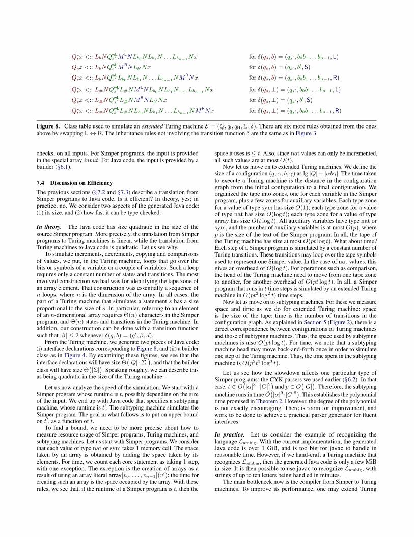
Consider an extended Turing machine such that |β| = 1 wheneverδ(q, b) = (q′, β, d). It is easy to see that such an extended machinetrivially corresponds to a normal one. Accordingly, we translate suchan extended machine in exactly the same way as we would translatethe normal one. We only need to do something different for thosetransitions with |β| 6= 1. These differences are illustrated in Figure 8.Briefly, each β = b0 . . . bn−1 in the transition function results in astringLb0N . . . Lbn−1N of classes in the corresponding inheritancerule. The special case |β| = 1 is identical to the translation for non-extended transition functions.

This concludes our translation from Simper programs to Javacode. The Simper program halts if and only if the Java code type

QLsx <:: LbNQ

wLs′M

LNLb0NLb1N . . . Lbn−1Nx for δ(qs, b) = (qs′ , b0b1 . . . bn−1, L)

QLsx <:: LbNQ

wLs′M

RNLb′Nx for δ(qs, b) = (qs′ , b′, S)

QLsx <:: LbNQ

wLs′ Lb0NLb1N . . . Lbn−1NM

RNx for δ(qs, b) = (qs′ , b0b1 . . . bn−1,R)

QLsx <:: L#NQ

wLs′ L#NM

LNLb0NLb1N . . . Lbn−1Nx for δ(qs,⊥) = (qs′ , b0b1 . . . bn−1, L)

QLsx <:: L#NQ

wLs′ L#NM

RNLb′Nx for δ(qs,⊥) = (qs′ , b′, S)

QLsx <:: L#NQ

wLs′ L#NLb0NLb1N . . . Lbn−1NM

RNx for δ(qs,⊥) = (qs′ , b0b1 . . . bn−1,R)

Figure 8. Class table used to simulate an extended Turing machine E = (Q, qI, qH,Σ, δ). There are six more rules obtained from the onesabove by swapping L↔ R. The inheritance rules not involving the transition function δ are the same as in Figure 3.

checks, on all inputs. For Simper programs, the input is providedin the special array input . For Java code, the input is provided by abuilder (§6.1).

7.4 Discussion on EfficiencyThe previous sections (§7.2 and §7.3) describe a translation fromSimper programs to Java code. Is it efficient? In theory, yes; inpractice, no. We consider two aspects of the generated Java code:(1) its size, and (2) how fast it can be type checked.

In theory. The Java code has size quadratic in the size of thesource Simper program. More precisely, the translation from Simperprograms to Turing machines is linear, while the translation fromTuring machines to Java code is quadratic. Let us see why.

To simulate increments, decrements, copying and comparisonsof values, we put, in the Turing machine, loops that go over thebits or symbols of a variable or a couple of variables. Such a looprequires only a constant number of states and transitions. The mostinvolved construction we had was for identifying the tape zone ofan array element. That construction was essentially a sequence ofn loops, where n is the dimension of the array. In all cases, thepart of a Turing machine that simulates a statement s has a sizeproportional to the size of s. In particular, referring to an elementof an n-dimensional array requires Θ(n) characters in the Simperprogram, and Θ(n) states and transitions in the Turing machine. Inaddition, our construction can be done with a transition functionsuch that |β| ≤ 2 whenever δ(q, b) = (q′, β, d).

From the Turing machine, we generate two pieces of Java code:(i) interface declarations corresponding to Figure 8, and (ii) a builderclass as in Figure 4. By examining these figures, we see that theinterface declarations will have size Θ

(|Q|·|Σ|

), and that the builder

class will have size Θ(|Σ|). Speaking roughly, we can describe this

as being quadratic in the size of the Turing machine.

Let us now analyze the speed of the simulation. We start with aSimper program whose runtime is t, possibly depending on the sizeof the input. We end up with Java code that specifies a subtypingmachine, whose runtime is t′. The subtyping machine simulates theSimper program. The goal in what follows is to put on upper boundon t′, as a function of t.

To find a bound, we need to be more precise about how tomeasure resource usage of Simper programs, Turing machines, andsubtyping machines. Let us start with Simper programs. We considerthat each value of type nat or sym takes 1 memory cell. The spacetaken by an array is obtained by adding the space taken by itselements. For time, we count each core statement as taking 1 step,with one exception. The exception is the creation of arrays as aresult of using an array literal array[v0, . . . , vn−1](v′): the time forcreating such an array is the space occupied by the array. With theserules, we see that, if the runtime of a Simper program is t, then the

space it uses is≤ t. Also, since nat values can only be incremented,all such values are at most O(t).

Now let us move on to extended Turing machines. We define thesize of a configuration (q, α, b, γ) as lg |Q|+ |αbγ|. The time takento execute a Turing machine is the distance in the configurationgraph from the initial configuration to a final configuration. Weorganized the tape into zones, one for each variable in the Simperprogram, plus a few zones for auxiliary variables. Each type zonefor a value of type sym has size O(1); each type zone for a valueof type nat has size O(log t); each type zone for a value of typearray has size O(t log t). All auxiliary variables have type nat orsym, and the number of auxiliary variables is at most O(p), wherep is the size of the text of the Simper program. In all, the tape ofthe Turing machine has size at most O(pt log t). What about time?Each step of a Simper program is simulated by a constant number ofTuring transitions. These transitions may loop over the tape symbolsused to represent one Simper value. In the case of nat values, thisgives an overhead of O(log t). For operations such as comparison,the head of the Turing machine need to move from one tape zoneto another, for another overhead of O(pt log t). In all, a Simperprogram that runs in t time steps is simulated by an extended Turingmachine in O(pt2 log2 t) time steps.

Now let us move on to subtyping machines. For these we measurespace and time as we do for extended Turing machine: spaceis the size of the tape; time is the number of transitions in theconfiguration graph. As explained in Section 5 (Figure 2), there is adirect correspondence between configurations of Turing machinesand those of subtyping machines. Thus, the space used by subtypingmachines is also O(pt log t). For time, we note that a subtypingmachine head may move back-and-forth once in order to simulateone step of the Turing machine. Thus, the time spent in the subtypingmachine is O(p2t3 log3 t).

Let us see how the slowdown affects one particular type ofSimper programs: the CYK parsers we used earlier (§6.2). In thatcase, t ∈ O

(|α|3 · |G|2

)and p ∈ O

(|G|). Therefore, the subtyping

machine runs in time O(|α|9 ·|G|8

). This establishes the polynomial

time promised in Theorem 2. However, the degree of the polynomialis not exactly encouraging. There is room for improvement, andwork to be done to achieve a practical parser generator for fluentinterfaces.

In practice. Let us consider the example of recognizing thelanguage Lambig. With the current implementation, the generatedJava code is over 1 GiB, and is too big for javac to handle inreasonable time. However, if we hand-craft a Turing machine thatrecognizes Lambig, then the generated Java code is only a few MiBin size. It is then possible to use javac to recognize Lambig, withstrings of up to ten letters being handled in minutes.

The main bottleneck now is the compiler from Simper to Turingmachines. To improve its performance, one may extend Turing

machines further; for example, with a ‘go to marker’ primitiveoperation. Or, perhaps one might find a reduction that does not useTuring machines as an intermediate representation.

8. DiscussionDoes the reduction from Section 5 apply to other languages likeC] and Scala? No. Both of them adopted the recursive–expansiverestriction of (Viroli 2000), as recommended by (Kennedy andPierce 2007). Roughly, this restriction is a syntactic check thatsucceeds if and only if our Turing tapes are bounded. For boundedtapes, the halting problem is decidable.

What is the practical relevance of Theorem 1? For C, there existsa formally verified type checker in CompCert (Leroy 2009, ver-sion 2.5). For Java, Theorem 1 implies that a formally verified typechecker that guarantees partial correctness cannot also guaranteetermination. In most applications, partial correctness suffices, butnot so in security critical applications (where users are malicious),nor in mission critical applications (where nontermination is costly).Since there cannot be a totally correct Java type checker, Theorem 1strengthens the motivation behind research into alternative typesystems, such as (Greenman et al. 2014) and (Zhang et al. 2015).

It is perhaps difficult to imagine how could the Java type checkerbe the target of a security attack. However, consider a scenario inwhich generics are reified, as has been discussed for a future versionof Java. In that case, one needs to perform subtype checks at runtimeto implement instanceof. In other words, instanceof becomesa potential security vulnerability for any Java program that uses it.A simple fix might be to change the specification of instanceofto allow it to throw a timeout exception. Let us hope that a bettersolution exists. Similar problems occur if one tries to add gradualtyping to Java.

What is the practical relevance of Theorem 2? On the one hand,it hints that it may be possible to implement parser generators forfluent interfaces, which would make it easier to embed domainspecific languages in Java. On another hand, the techniques used inits proof may be reusable for encoding other computations in Java’stype system.

To summarize, Theorems 1 and 2 have practical implications:

1. A formally verified type checker for Java can guarantee partialcorrectness but cannot guarantee termination.

2. If reified generics are added to Java, then one needs to find somesolution for not turning instanceof into a security problem.Similarly, any technique (such as gradual typing) that involvessubtype checking at runtime is a potential security problem.

3. It may be possible to develop parser generators that help withembedding domain specific languages in Java.

Still, Theorem 1 is primarily of theoretical interest: It strengthensthe best lower bound on Java type checking (Gil and Levy 2016), andfinally answers a question posed almost a decade ago by (Kennedyand Pierce 2007).

9. Related WorkJava’s type system is not only undecidable, but also unsound (Aminand Tate 2016). Many other languages have undecidable type sys-tems: Haskell with extensions (Wansbrough 1998; Sulzmann et al.2007), OCaml (Lillibridge 1997; Rossberg 1999), C++ (Veldhuizen2003), and Scala (Bjarnason 2009; Odersky 2016), to name a few.It is often the case that undecidable type systems are a fun play-ground for metaprogramming. For example, in Haskell, undecidableinstances are useful for deriving type classes (Weirich 2006); and,in C++, libraries like Boost.Hana (Dionne 2016) allow one to easily

write (mostly) functional programs that run at compile time. WillJava’s type system become a playground for metaprogramming?(Gil and Levy 2016) and Theorem 2 show that it is possible inprinciple. It remains to be seen whether it is possible in practice.

On the theory side, perhaps the closest result is that subtypechecking is undecidable in F<: (Pierce 1994). That proof has somehigh level similarities with the one presented here: it considers adeterministic type system, and shows a reduction from (a kind of)Turing machines, by using an intermediate formalism. We also knowthat System F is undecidable (Wells 1999). But, its subset known asHindley–Milner is decidable, in fact type inference is DEXPTIME-complete (Mairson 1990).

Why should we care about toy type systems like F<: and that ofSystem F ? Because real type systems like Java’s are too difficultfor humans to reason about. There are three ways in which one cansettle the decidability of type checking for a real world language X:(i) find a simple type system that is less expressive than that of X,and show it is undecidable; (ii) find a simple type system that is moreexpressive than that of X, and show that it is decidable; or (iii) tacklethe original type system but do a mechanically verified proof.For (iii), a huge effort is required. This paper falls in category (i).The simple type system is neither F<: nor System F . Instead, itis taken from (Kennedy and Pierce 2007). Kennedy and Piercestudy several variations of the type system they propose. Alas, thosevariations they prove decidable are less expressive than Java, andthose variations they prove undecidable are not less expressive thanJava. The variant they prove undecidable allows classes of arity 2and multiple instantiation inheritance, which in our setting translatesto having nondeterministic subtyping machines. Their reduction isfrom PCP. They conjecture that multiple instantiation inheritance isessential for undecidability. That turns out not to be the case.

10. ConclusionIt is possible to coerce Java’s type checker into performing anycomputation. This opens possibilities for use and abuse.

AcknowledgmentsThe problem was brought to my attention by (Lippert 2013), andit started to look very interesting after I read the result of (Gil andLevy 2016). Stefan Kiefer, Rasmus Lerchedahl Petersen, JoshuaMoerman, Ross Tate, and Brian Goetz provided feedback on earlierdrafts. Nada Amin answered my questions about Scala. HongseokYang encouraged me to write a proper paper.

ReferencesN. Amin and R. Tate. Java and Scala’s type systems are unsound: The

existential crisis of null pointers. In OOPSLA, 2016.R. O. Bjarnason. More Scala typehackery.

https://apocalisp.wordpress.com/2009/09/02/ (see alsohttps://michid.wordpress.com/2010/01/29), 2009.

A. Breslav. Mixed-site variance in Kotlin.http://blog.jetbrains.com/kotlin/2013/06/mixed, 2013.

B. Courcelle. On jump-deterministic pushdown automata. MathematicalSystems Theory, 1977.

L. Dionne. Boost.Hana. http://boostorg.github.io/hana, 2016.Y. Gil and T. Levy. Formal language recognition with the Java type checker.

In ECOOP, 2016.O. Goldreich. Computational complexity: a conceptual perspective.

Cambridge University Press, 2008.J. Gosling, B. Joy, G. Steele, G. Bracha, and A. Buckley. The Java language

specification, 2015. Java SE 8 Edition.B. Greenman, F. Muehlboeck, and R. Tate. Getting F-bounded

polymorphism into shape. In PLDI, 2014.

R. Grigore. Parser generator for fluent interfaces.http://rgrig.appspot.com/javats, 2016.

J. E. Hopcroft and J. D. Ullman. Introduction to Automata Theory,Languages, and Computation. Addison–Wesley, 1979.

A. J. Kennedy and B. Pierce. On decidability of nominal subtyping withvariance. In FOOL, 2007.

D. E. Knuth. On the translation of languages from left to right. Informationand Control, 1965.

M. Lange and H. Leiß. To CNF or not to CNF? An efficient yet presentableversion of the CYK algorithm. Informatica Didactica, 2009.

X. Leroy. Formal verification of a realistic compiler. CACM, 2009.M. Lillibridge. Translucent Sums: A Foundation for Higher-Order Modules.

PhD thesis, CMU, 1997.E. Lippert. A simple problem whose decidability is not known. Theoretical

Computer Science Stack Exchange, 2013.http://cstheory.stackexchange.com/q/18866.

H. G. Mairson. Deciding ML typability is complete for deterministicexponential time. In POPL, 1990.

M. Odersky. Scaling DOT to Scala – soundness. http://scala-lang.org/blog/2016/02/17/scaling-dot-soundness.html, 2016.

B. C. Pierce. Bounded quantification is undecidable. Information andComputation, 1994.

A. Rossberg. Undecidability of OCaml type checking. Caml mailing list,1999.

http://caml.inria.fr/pub/old_caml_site/caml-list/1507.html.M. Sulzmann, G. J. Duck, S. L. P. Jones, and P. J. Stuckey. Understanding

functional dependencies via constraint handling rules. J. Funct.Program., 2007.

R. Tate, A. Leung, and S. Lerner. Taming wildcards in Java’s type system.In PLDI, 2011.

A. M. Turing. On computable numbers, with an application to theEntscheidungsproblem. J. of Math, 1936.

T. L. Veldhuizen. C++ templates are Turing complete. Technical report,Indiana University, 2003.

M. Viroli. On the recursive generation of parametric types. Technical report,University of Bologna, 2000.

K. Wansbrough. Instance declarations are universal.http://www.lochan.org/keith/publications/undec.html(see also https://wiki.haskell.org/Type_SK), 1998.

S. Wehr and P. Thiemann. On the decidability of subtyping with boundedexistential types. In APLAS, 2009.

S. Weirich. RepLib: a library for derivable type classes. In Haskell, 2006.J. B. Wells. Typability and type checking in System F are equivalent and

undecidable. Annals of Pure and Applied Logic, 1999.Y. Zhang, M. C. Loring, G. Salvaneschi, B. Liskov, and A. C. Myers.

Lightweight, flexible object-oriented generics. In PLDI, 2015.