jane sneddon little - federal reserve bank of boston sneddon little economist, federal reserve bank...

Jane Sneddon Little

Economist, Federal Reserve Bank ofBoston. The author has benefited agreat deal from the comments andsuggestions of several colleagues, butparticularly Richard W. Kopcke andJeffrey C. Fuhrer. Lawrence D. Her-man, Michael D. Jud, and Garrett J.Solomon provided excellent researchassistance. The author is particularlygrateful to Michael ]ud for his substan-tive contributions to the statisticalzvork.

T hroughout the recent recession and ensuing period of barelyperceptible growth, manufacturers have described their invento-ries as remarkably lean. Since inventories usually rise sharply

relative to sales during economic downturns, these manufacturers havehastened to add, with some pride, that their well-controlled stocksresult from considerable management effort. Many of these firmsreportedly changed their approach to inventory management during the1980s. Sometimes these efforts required substantial investments toinstall new systems; often the effort is considered incomplete.

A glance at inventory-to-sales trends supports these manufacturers’claims about the ratios’ "historically" low levels--by recent standards, atany rate. Thus, even though inventory accumulations and liquidationstypically aggravate business cycles,1 early in the recent downturn manyobservers suggested that these unusually lean inventory-to-sales ratioswould insure a rapid and robust recovery from a short, mild recession.In the event, these observers have been disappointed in the nature ofthe recovery.

Despite media commentary and manufacturers’ protestations,many analysts remain skeptical that the relationship between invento-ries and sales has changed significantly once, for example, differences inthe outlook for inflation are taken into account. And, indeed, muchcurrent research has uncovered little evidence of any structural change.For example, in a relatively recent review of the inventory literature,Alan Blinder and Louis Maccini address the issue by saying that"despite the alleged revolution in inventory practices brought about bycomputerization, the economy-wide ratio of real inventories to real saleshas been trendless for 40 years" (1991, p. 75).2 Similarly, in discussingthe trend toward more frequent deliveries from U.S. auto suppliers toassemblers, Womack, Jones, and Roos of MIT’s International MotorVehicle Program describe the change as "simply an attempt by assem-blers to shift costs to their suppliers," with little net reduction in

inventories for the U.S. industry as a whole (1990,p. 160).3 These differing conclusions may simplyreflect different perspectives, since individual firmsor industries could make major strides in reducingtheir own inventory-to-sales ratio without the econ-omy as a whole achieving significant savings inrequired stocks.

This article begins by describing recent trends ininventory management at the firm level. It thenpresents statistical evidence supporting the manufac-turers’ claims that something is different. During the1980s a structural change in the relationship between

This article will argue that thetransition to improved inventory

management is exerting anoticeable drag on current

economic growth.

inventories and sales does seem to have occurred,most noticeably within the manufacturing sector, butalso in the economy as a whole. A final sectionexplores the implications of these structural changesfor the pace of current economic growth. Since initi-atives to reduce inventories both reflect and permitgreater efficiency, in the long run they suggest en-hanced U.S. economic welfare. Nevertheless, con-trary to the optimists who thought that tight inven-tories implied a robust recovery, this article will arguethat the transition to improved inventory manage-ment is exerting a noticeable drag on current eco-nomic growth. In addition to providing evidence thata structural change is under way, this article alsopresents indications that the transition is not yetcomplete. Accordingly, the article concludes by spec-ulating that the ongoing adoption of lean inventorypractices represents a structural impediment to arapid recovery.

Setting the Stage: Why the 1980s?Pushed by increased competition and pinched

profit margins and aided by the falling cost of newtechnology, most U.S. firms in manufacturing andtrade made some effort during the 1980s to reduce the

resources devoted to holding and handling invento-ries. One contributory development was the sharprise in real interest rates from historically low levels inthe late 1970s to much higher levels in the early 1980s.Because high real interest rates increase the cost ofholding inventory, this change undoubtedly encour-aged firms to find ways to eliminate excess stocks. Inaddition, between 1980 and 1985, the dollar appreci-ated by 50 percent in the foreign exchange markets.This appreciation exposed U.S. producers to greatlyincreased foreign competition, again forcing them toreexamine their operating methods. At.the sametime, the availability of small computers and otherinformation processing technology was exploding,while the real cost of this equipment was decliningrapidly. In other words, during the 1980s incentiveand opportunity converged to persuade U.S. busi-nesses to find new ways to manage their inventories.

Undoubtedly because the Japanese auto firmshad grabbed U.S. market share during the oil crises ofthe 1970s and then, in 1982, began setting up com-peting plants onshore, U.S. auto companies madesome of the first moves towards adopting new meth-ods of inventory control. In 1984, for example, Gen-eral Motors and Toyota opened the New UnitedMotor Manufacturing Inc. (NUMMI) plant in Free-mont, California. This joint venture typified the U.S.auto industry’s somewhat scattered efforts to experi-ment with Japanese lean production methods in theUnited States (Womack, Jones, and Roos 1990). (Seethe Box for a brief description of "lean manufactur-ing," as developed at Toyota.)

Wholesalers and retailers appear to have focusedon inventory reduction somewhat later than manu-facturers, even though the trade sector almost tripledits investment in information processing equipment4between the late 1970s and the early 1980s (Hender-

1 In the United States, but not necessarily in Japan. See West(1991).2 The 40-year period seemingly covered the years 1949 to 1989.

In another recent study finding no evidence of structural change,Kenneth D. West wrote, "But over the longer 1967-1987 period, wesee . . . that there has been no secular movement in any of the(inventory-to-sales) ratios in the U.S." (West 1991, p. 9).

3 By contrast, two recent papers that do find evidence that theinventory-to-sales (or output) ratio has declined over time or withthe advent of computerized inventory control are Cuthbertson andGasparro (1992), who looked at data for the United Kingdom, andBechter and Stanley (1992), who found clear evidence of improvedinventory control in U.S. manufacturing but mixed results inwholesale and retail trade.

4 Information processing equipment covers everything fromcash registers to computers to point-of-sale scanning equipment.

38 November/December 1992 New England Economic Review

Lean Production

The lean approach to manufacturing was de-veloped in the 1950s at Toyota by Eiji Toyodaand Toyota’s chief production engineer, TaiichiOhno, in response to conditions in post-WorldWar II Japan. At that time, the Japanese automarket was small, the Japanese manufacturershad little capital, and the American occupationforces greatly restricted management’s right tolay off workers. Because Ohno’s capital budgetrequired that most of a car be stamped from justa few press lines, he developed simple die-changetechniques that permitted production workers tochange dies every two or three hours in a processthat took three minutes. In the United States,by contrast, presses were plentiful and dedicatedto specific tasks, and die changes were madeonly every few months or years by die changespecialists who usually took a full day to make theswitch.

Forced by their lack of capital to rely on just afew presses, Ohno then discovered that producing

small batches of stampings actually saved money.Making small batches eliminated the cost of carry-ing huge inventories of work in process, andmaking only a few parts before assembling theminto finished cars caused stamping mistakes toshow up right away.

Other hallmarks of lean production includeasking teams of workers to take responsibility forspotting and correcting quality and other problemsand for suggesting ways to improve the produc-tion process. Lean supply is another key ingredi-ent. In lean supply, assemblers and suppliers worktogether to lower costs and improve quality. In-deed, first tier suppliers participate in the design ofnew products. In addition, the flow of parts be-tween suppliers and assembler is coordinated sothat the supplies arrive "just-in-time." The signal-ing mechanism is the container carrying parts.When the parts are used up, the container returnsto the supplier, thereby signaling the need formore parts.

son 1992). Indeed, it was not until a 1987 canoe tripthat Wal-Mart’s Sam Walton and Procter & Gambleexecutive Lou Pritchett realized that their companieshad been communicating "by slipping notes underthe door .... No sharing of information, no plan-ning together, no systems coordination. We weresimply two giant entities going our separate ways,oblivious to the excess costs created by this obsoletesystem" (Walton 1992, p. 186).

Shortly thereafter, Procter & Gamble and Wal-Mart managers developed an innovative system forexchanging sales and inventory data via computer.According to Mr. Pritchett, "We broke new groundby using information technology to manage our busi-ness together, instead of just to audit it" (Walton1992, p. 187). Since then, Wal-Mart has used thisrelationship as a model and has pressed other sup-pliers to adopt electronic data interchange (EDI) aswell.

Accordingly, the years 1982 and 1987 seem tobracket the start of serious efforts to eliminate wastein U.S. inventories. In 1982 the arrival of Honda withthe first Japanese transplant caught the U.S. manu-facturers’ attention, while Sam Walton and LouPritchett’s 1987 canoe trip led to major changes in

retailing and in the supply system linking the twosectors.

New Approachbs to Inventory ManagementManufacturers have taken a variety of approaches

to cutting inventories, with varying degrees of success.Some firms have focused on inventory reduction di-rectly; in other cases, declines in the inventory-to-sales ratio have accompanied efforts to implement aquality or time management program or a movetoward lean production. Wherever the emphasis hasbeen placed, quality, time, and inventory behaviorare clearly closely connected. Just as operating withslim inventories requires promptly delivered partswith few defects, so, conversely, high-quality pro-duction reduces inventories of work-in-process,s

s How important reducing defects can be is illustrated byToyota’s savings. Typically, U.S. mass-production auto plantsdevote 13 percent of their space to the rework area and up to aquarter of the total hours required to build a car to fixing mistakes.By contrast, Japanese assembly plants currently use 4 percent oftheir space and almost no time at all for rework (Womack, Jones,and Roos 1990, p. 92).

November/December 1992 New England Economic Review 39

Manufacturing

Manufacturing approaches to inventory controltend to fall into two categories that are often viewedas alternatives but can in fact be combined to advan-tage.6 More widely used in this country is materialsrequirements planning or materials resource plan-ning (MRP or MRPII), a computer-driven systemwhich initiates production in anticipation of forecastdemand. By contrast, just-in-time (JIT) starts produc-tion in reaction to current conditions on the shopfloor. As an example of the difference, McDonald’sruns a JIT shop, while a caterer must use an MRPII-type system. Like MRPII, just-in-time aims to deliverwhatever is needed when it is needed; it seeks toeliminate delays and confusion and to save the re-sources that would otherwise be devoted to storingand moving excess work-in-process or buffer stock.But, JIT does not recognize future events.

By contrast, MRP starts with expected sales andreleases orders for the required parts according topredetermined lead times. Relative to JIT, MRP isexpensive, since companies must purchase the com-puter systems on which the approach is based andtrain workers to use them. In addition, the system’sassumption of fixed (but adjustable) productionmethods and lead times contrasts with the JIT focuson constant improvement.

JIT works best when demand is smooth; whendemand varies, JIT is less likely than MRP to operatein a stockless manner. Long before JIT was widelyknown in this country, Forrester (1961) had alreadyshown that the more variable the demand conditions,the more inventory a distribution system needs.Indeed, the current slowdown in Japanese economicactivity may expose the Japanese JIT system to un-usually severe stress.7

The Retail Equivalent

The retailers’ equivalent to MRPII or JIT is QuickResponse, a business strategy intended to cut thecosts associated with managing inventory, while re-ducing stockouts and improving customer service.According to an Andersen Consulting study, in 1988some 36 percent of U.S. vendors of general merchan-dise were using the Universal Product Code, a firststep in implementing a Quick Response Program,while just 10 percent of the survey respondents wereexchanging data electronically to some degree(Andersen Consulting 1988). Three years later,Andersen Consulting found, almost three-quarters of

Florida retailers were "in the process of" implement-ing Quick Response in their operations (Chain StoreAge Executive 1991). Nevertheless, as the same issueof Chain Store Age Executive points out, while mostretailers have begun to install Quick Response tech-nologies, few have established the vendor-supplierpartnerships required to shorten the inventory pipe-line significantly, probably because such strategiesrequire difficult cultural changes. As an example ofsuch resistance, it took Federated Department Stores’

Few retailers have established thevendor-supplier partnerships

required to shorten the inventorypipeline significantly.

bankruptcy to get its divisions to cooperate in devel-oping a centralized inventory management system.The eight divisions had long opposed such a step aslargely useless, since each chain has its own person-ality and market niche (Strom 1992).

The new technologies that permit Quick Re-sponse include bar coding and point of sale scanning,which allow retailers to track merchandise to theitem-size-color level, and electronic data interchange(EDI), which permits retailers and suppliers to sharesales data and business documents. These technolo-gies let retailers increase checkout productivity, re-duce stockouts and markdowns, and end the need toreprice merchandise for promotions. They also im-prove distribution center productivity by eliminatingmanual receiving and checking procedures. In addi-tion, automatic replenishment systems can continu-ously compare inventory, order-to-delivery time lags,and expected sales to generate purchase orders forspecific stores and items. EDI speeds the flow andincreases the accuracy of such transactions as pur-

6 Much of this section is based on Karmarkar (1989).7 Heretofore, whenever the Japanese auto makers have faced

a decline in domestic demand, they have maintained relativelysmooth output growth by expanding exports (Womack, Jones andRoos 1990). This slowdown may be the first in which internationalpolitics and the Japanese auto makers’ competitive position willnot permit this solution. Accordingly, Japanese assembler-supplierrelations are showing unusual signs of strain (Pollack 1992).Perhaps the Japanese will want to incorporate elements of MRPIIinto their JIT systems.


chase orders, advanced shipping notices, and in-voices. This type of communication between retailersand suppliers reduces clerical, data entry, postage,handling, and form printing costs, while improvingaccuracy. It also reduces inventory lead times andcarrying costs. As Forrester has shown, reducingdelays can actually cut the amount of inventoryneeded for the pipeline.

Accomplishments of Individual FirmsWhat have firms introducing these new ap-

proaches to inventory management accomplished?This section provides a small sample of individualcompany experiences. Its aim is to suggest by anec-dote that companies trying to reduce the resourcesdevoted to holding and handling inventory havesucceeded in reaping some significant savings.

In 1982 Xerox began to feel increased pressurefrom Japanese competitors and was losing marketshare. At that time, the company was buying mate-rials representing 80 percent of its manufacturingcosts from 5,000 suppliers. Seeking to reduce thesecosts, the company narrowed its supplier base to 400and began training the selected suppliers in statisticalprocess and statistical quality control programs andjust-in-time manufacturing techniques. Xerox alsoincluded suppliers in the design of new products. Asa result, from 1981 to 1984, net product costs werereduced by close to 10 percent a year, rejects ofincoming materials were reduced by 93 percent, andproduction lead times were reduced from 52 weeks to18 weeks (Burt 1989).

Similarly, in 1986 Northern Telecom Inc. decidedto improve its competitiveness by "squeezing time"out of its operations. Using a quality managementprogram, the company reduced manufacturing inter-vals by two-thirds. In the area of procurement, itinstalled a JIT inventory system on the shop floor andworked closely with "certified," single-source suppli-ers to make sure that the materials received meetNorthern Telecom’s quality standards and arrive ontime. As a result, at the Research Triangle ParkDivision, which makes large digital central officeswitching systems, the receiving cycle has been cutfrom three weeks to four hours, the incoming inspec-tion staff has fallen by hall and shop floor problemscaused by defective materials have almost vanished(Merrills 1989).

Looking abroad, Unipart, a British auto partmaker, adopted lean manufacturing methods and

increased inventory turnover from three to four timesa year to 27 times a year. Stocks of parts and finishedproducts once occupied 80,000 square feet; they nowoccupy 28,000 square feet, a 65 percent reduction("Unipartners" 1992). More widely, auto parts sup-pliers using a lean approach report declines of asmuch as 50 percent in the amount of space requiredfor production and increases in productivity as highas 30 percent (Womack, Jones, and Roos 1990). (Foradditional examples, see the Box on page 42.

Of course, these examples reflect the efforts ofjust a few companies that have embraced lean man-ufacturing with enthusiasm and success. What hashappened in the economy as a whole?

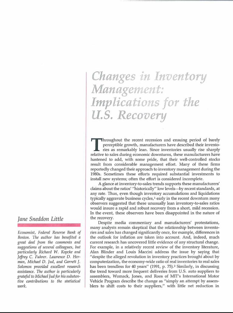
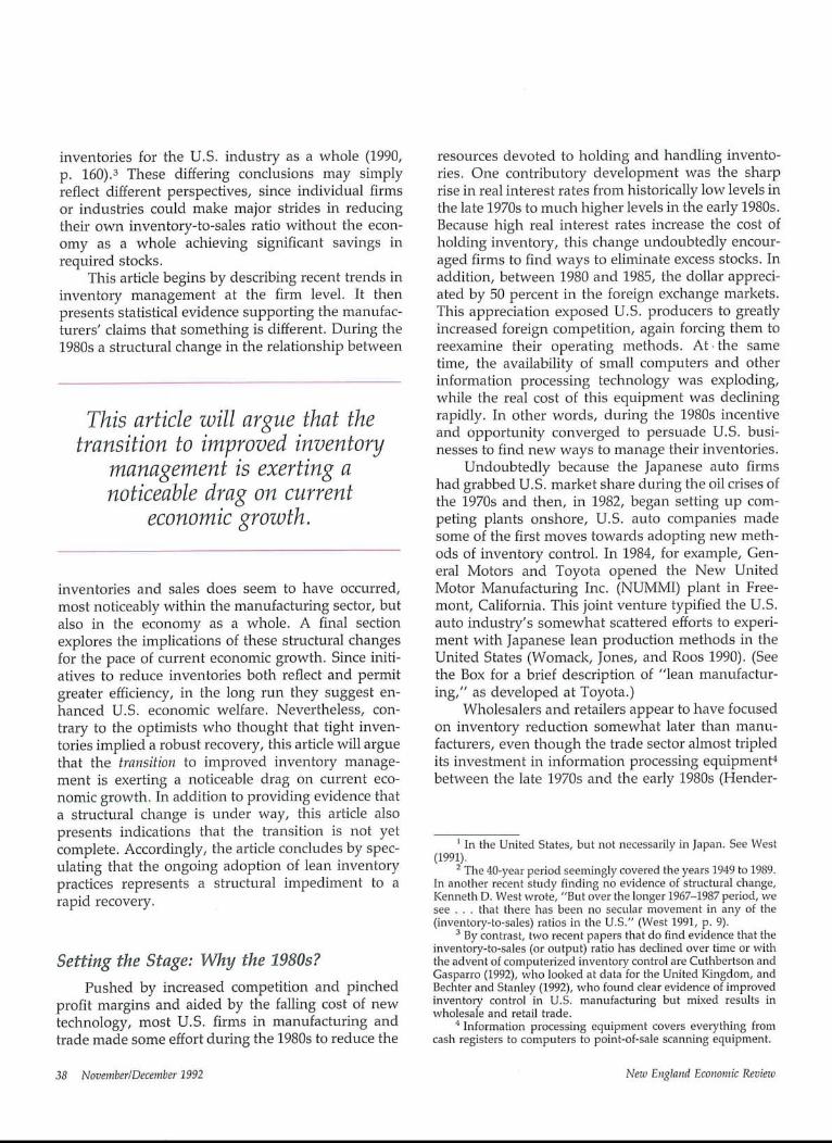
The Broader ViewLooking at Figures 1 and 2, which show inven-

tory-to-sales ratios for the major sectors of the econ-omy, suggests that something may have "happened"in the 1980s. (Appendix Figures A-1 through A-3provide a more detailed picture.) Since the end of1982, this ratio has fallen--modestly for the economyas a whole, sharply for durable goods manufactur-ing.s By exception, retail inventories trended upslightly, but not enough to offset all of the gains madein manufacturing. The charts also show that whileinventories jumped up slightly in relation to salesduring the recent recession, the ratio did not continueclimbing throughout the downturn as has been thenorm in previous cycles. Indeed, in manufacturingand trade, the inventory-to-sales ratio averaged just1.46 during the recent recession, only slightly abovethe low point of 1.44 reached briefly in the nonreces-sionary first quarter of 1973. In the first quarter of1991, the inventory-to-sales ratio was 1.49, 10 percentbelow its average for the four previous cyclicaltroughs.

But do these changes necessarily reflect the ef-forts to cut inventories discussed above? After all, therecent recession was relatively mild, by official stan-

8 Inventories can be divided into five roughly equal parts.Retail and wholesale inventories each account for one-fifth of thetotal and are largely composed of finished goods. The three-fifthsof the total represented by manufacturing stocks are fairly evenlydivided between materials and supplies, work-in-process, andfinished goods. During the 1980s, these three types of manufac-turing inventories declined proportionately. This developmentshould help to convince doubters that the economy could havemade at least modest net reductions in inventories, since cuttingwork-in-process is fundamentally different from shifting stocks toand fro in the supply chain.


Figure 1

htventory-to-Sales RatiosManufacturing and Trade, and

Manufacturing

1967 1969 1971 1973 1975 1977 1979 1981 1983 1985 1987 1989 1991

Ouarlerly data, seasonally adjusledShaded areas represen! recessions.Source: U.S. Bureau of Economic Analysis.

Figure 2

Ratio3.0

2.5

2.0

1.5

1.0

Inventory-to-Sales Ratios inWholesale and Retail Trade

Based on 1982 Dollars

Retail Nondurable Goods

.5

Quarterly data, seasonally adjusted.Shaded areas represent recessions.Source: U.S. Bureau of Economic Analysis.

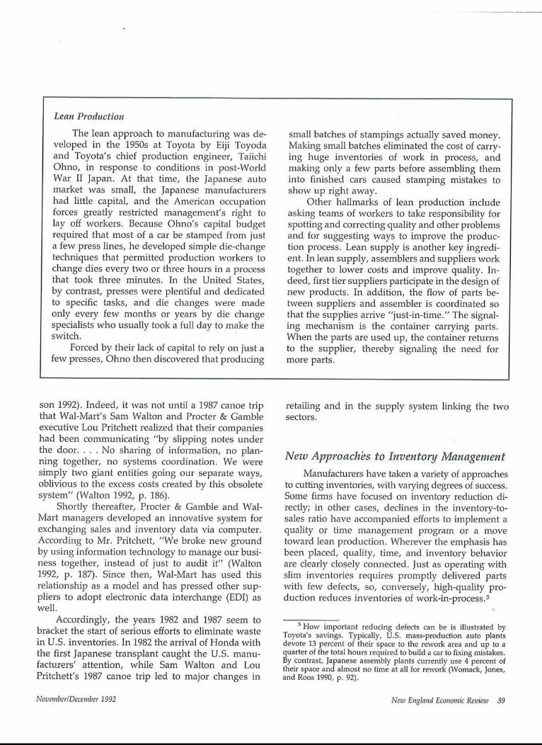
Further Examples of Individual Firm Accomplishmentsvia Lean Inventomd Management

As another example of individual companyefforts, in 1987 Hewlett-Packard was receiving just21 percent of its deliveries on time. The firm spentmany hours devising schemes to keep productionlines operating in the face of delays, while earlydeliveries required costly storage and control. Un-clear communications turned out to be one of themain problems; the supplier did not always knowwhether the date on the purchase order was theshipment date or the delivery date. Accordingly,Hewlett-Packard began using electronic purchaseorders that flow directly from HP’s computers tothe suppliers’ open-order management systems.Two years later, 51 percent of deliveries were ontime. As a consequence the production line stopsless frequently, and inventory expenses are down(Burt 1989).

Very recently, NCR-Ithaca (New York), in thecomputer printer industry, used JIT methods tocut on-hand inventory from 110 days to 21 days.

Work-in-process was cut by 80 percent (Saxon-house 1991). And, according to an April 1992 pressrelease, Kaye Instruments of Bedford, Massachu-setts implemented a full MRP system in 1991 andreduced net inventory by one-third while increas-ing shipments by 7 percent.

Finally, in the retail sector, Designs Exclu-sively Levi Strauss & Company, an apparel chainbased in Chestnut Hill, Massachusetts has estab-lished a Quick Response-EDI partnership with itsone vendor, Levi Strauss. The chain provides LeviStrauss with a frequently adjusted desired stocklevel for each item (including size and color) and aweekly sales data file. Levi Strauss compares saleswith desired stock levels and automatically sendsreplenishments direct to each store. The chain’schief financial officer estimates that this system hasreduced inventories by as much as 15 percentwhile stockouts have declined dramatically (ChainStore Age Executive).


dards, while expected inflation has declined mark-edly over the decade. Other constraints equal, rapidinflation is generally thought to encourage higherinventories, because firms may be able to buy or buildnow and sell later at a higher price. In such anenvironment, the difference between the purchaseand selling price may more than offset the cost ofcarrying the inventory. Moreover, as mentioned pre-viously, carrying costs, as measured by real interestrates, soared in the early part of the decade, therebyproviding another incentive to reduce stocks.

The Model

This study uses a set of simple regressions andstatistical tests to see whether the new inventorymanagement technologies have actually contributedto the apparent reduction in the inventory-to-salesratio to a statistically significant extent. The modeltested is a relative of that commonly used in eco-nomic studies, except that here the dependent vari-able is the inventory-to-sales ratio, whereas moststudies seek to "explain" inventory investment:9

As is the case in these related models, the con-stant-dollar inventory-to-sales ratio at the end of agiven quarter is assumed to be positively related to itsvalue at the end of the previous quarter; because theinventory-to-sales ratio appears to adjust to changesin economic conditions rather slowly, the higher theratio in one quarter, the higher its value is likely to bein the following period. 10 Similarly, because invento-

9 Blinder and Maccini (1991) provide a thorough review of theeconomic literature.

10 In the economics literature, much attention is devoted to theplausibility of the surprisingly long inventory adjustment periodsfound in most empirical studies. Since the entire adjustmentrequired usually amounts to a couple of days’ output, it may seempuzzling that the adjustment appears to get stretched out overseveral months. However, in his 1961 textbook, Jay Forresterpointed out that the more gradually a producer adjusts actualinventories to desired levels, the less production variability thefirm will experience.

Forrester also addressed another issue that has puzzled manyeconomists: why output is more variable than sales when produc-ers hold inventories for "production smoothing" purposes. AsForrester explains, producers and retailers set targets or limits forinventories. The lower limit is set to avoid halting the productionline or allowing stockouts; space constraints determine the upperlimit. Accordingly, even though sellers use inventories to absorban initial demand shock, production will still be more variable thansales, because all the players along the supply chain will adjusttheir reorder rate to meet the new level of demand as well as torestore their inventories to desired levels. In general, the longer thetime delay between final sale and replacement production or themore complex the pipeline, the greater will be the variability inproduction vis-a-vis sales.

ries change more slowly than sales, the inventory-to-sales ratio is expected to have a negative relationsl-fipwith the growth in sales in recent quarters. That is,the faster sales were growing in the previous threequarters, the lower the current inventory-to-salesratio is likely to be. Unexpected changes in thegrowth in sales, measured in this article by thegrowth in the current quarter minus the growth inthe previous period, also contribute to unplannedchanges in stocks; thus, a slowdown in the pace ofsales in the current quarter is expected to lead to anincrease in the inventory-to-sales ratio.11

Inventory behavior is also believed to reflectinflationary expectations and the cost of carryinginventories. Previous investigators have determinedthat these variables should enter the equation sepa-rately rather than combined in the form of the realinterest rate. (See Akhtar 1983, for instance.) Onereason for this strategy is that current carrying costs(represented by nominal short-term interest rates) areknown precisely by corporate decisionmakers andclearly (theoretically, if not empirically) have a nega-tive relationship with a firm’s desire to hold stocks.By contrast, future inflation must be estimated and islikely to show a positive association with buildinginventory, as mentioned above.12 In this study, thechange in the short-term interest rate from the previ-ous to the current quarter performed better than the

,1 While modeling expected and unexpected changes in salesalways presents challenges, the approach used in this article isadmittedly not completely orthodox. Cuthbertson and Gasparro(1992), for example, use a variance rather than a difference tomeasure unexpected changes in output (sales). Moreover, equa-tions explaining inventory investment often use lagged changes insales to represent sales expectations. In this paper, looking at theinventory-to-sales ratio, however, the coefficient on the distributedlag of changes in sales in the previous three quarters appears toreflect the relatively slow pace of adjustment to changes in salesrather than a change in expectations. Still, because of doubts aboutwhether current quarter changes in sales really represent sur-prises, Appendix Table A-3 presents the results of regressions inwhich expected sales, modeled following Bechter and Pollock(1981), were included in the equation. On the whole this forward-looking model produced results similar to the backward-lookingmodel presented in the text. In particular, investment in informa-tion processing equipment generally has a significant negative linkto the inventory-to-sales ratio. In addition, the coefficient onunexpected changes in sales (the change in sales during the currentquarter) usually remains significantly negative even when expectedsales are included. Nevertheless, because the backward-lookingequations "behaved" better as a whole, as was true for Cuthbert-son and Gasparro as well, the backward-looking equations appearin the text, while the forward-looking equations are relegated tothe Appendix.

~2 As will be discussed further below, however, work inprocess is likely to have a negative link with inflationary expecta-tions. In addition, retailers appear to follow a different purchasingstrategy from that pursued by manufacturers.

November/December 1992 New England Economic Reviao 43

level of the interest rate.13 Expected inflation is rep-resented by the pace of core inflation over the previ-ous year. More sector-specific measures of pricechange tended to perform less well.14

Finally, and key for the purposes of this article,the ratio of investment in information processingequipment to GDP, in 1982 dollars and lagged fourquarters, represented technological changes permit-ting new approaches to inventory management.15Although JIT systems do not require investment incomputers and scanners, interest in these organiza-tional approaches seemed to coincide, at leastroughly, with growing use of equipment-dependenttechniques like MRPII or Quick Response. For exam-ple, "just-in-time" first appears as a separate entry inthe periodicals indexes in 1984. The most obviousalternative to this approach, using a time trend or atime trend with a dummy after the end of 1982, isdifficult to interpret and less defensible. (That coursedid, however, produce roughly similar results, asshown in Appendix Table A-4.)

This model was applied to quarterly data from1968:I to 1990:IV. In addition, the same regressionswere run with the data divided into two subperiods,1968:I to 1982:III and 1982:IV to 1990:IV, in order totest whether structural changes have occurred. Theyear 1982 was chosen as the dividing point because ofthe behavior of the time series and because of pivotalevents like the establishment of the Honda plant andthe appearance of JIT in the periodicals indexes.

The Results

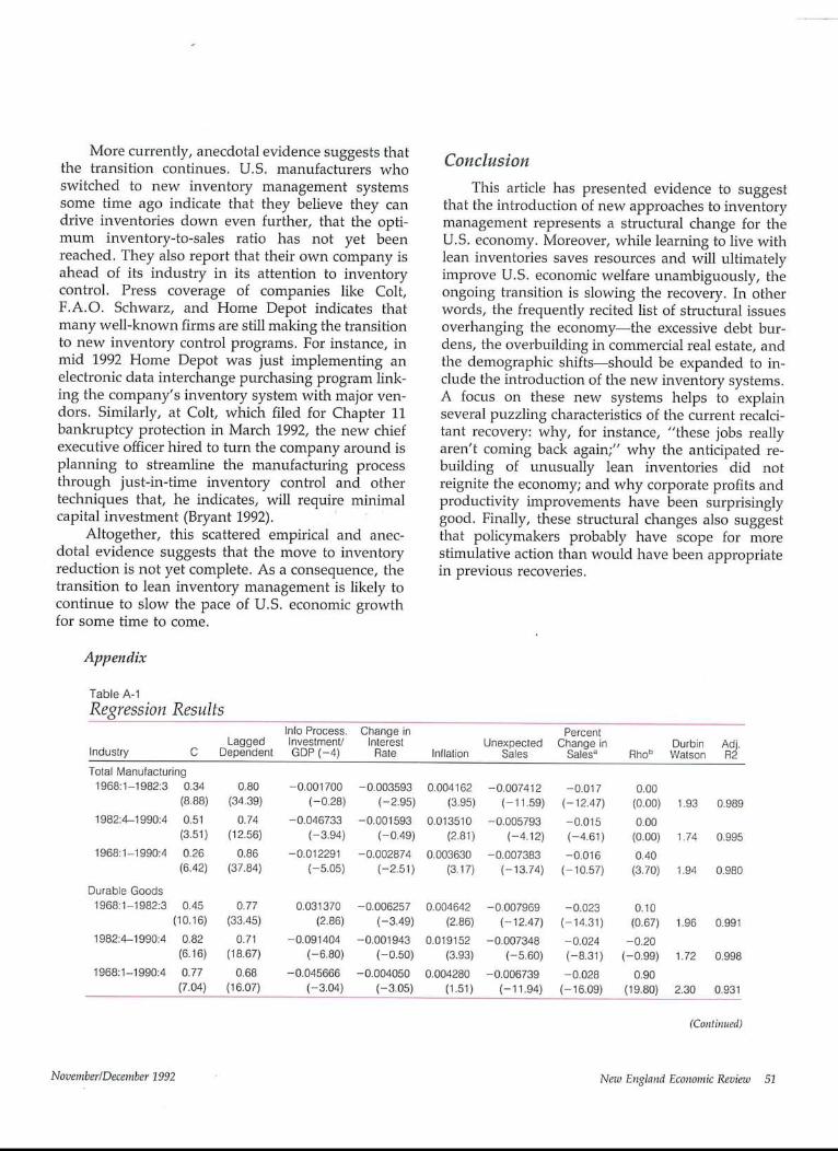
Because increases in the inventory-to-sales ratioin one industry or sector could offset decreases inothers, the key regression result for macroeconomicpurposes is that for manufacturing and trade. Ac-cordingly, Table 1 shows the results for manufactur-ing and trade alone while the results for the majorsubsectors and 15 individual industries are presentedin Appendix Table A-1.

In general, the explanatory variables have theexpected signs and are statistically significant at the 5percent level for the economy as a whole, for manu-facturing and durables and nondurables manufactur-ing, and for many of the individual manufacturingindustries. The variables that tend to be insignificantare usually inflationary expectations or the change ininterest rates, variables notorious for misbehaving ininventory models. (See, for example, Blinder andMaccini 1991, p. 82.) Most important for the focus ofthis article, however, investment in information pro-

Table 1Regression Results, Manufacturingand Trade

1968:1- 1982:4- 1968:1-1982:3 1990:4 1990:4

C .36 .74 .33(6.88) (3.09) (6.52)

Lagged Dependent .77 .58 .80(22.48) (4.70) (24.86)

Information Processing .00065 -.03511 -.00801Investment/GDP (-4) (.13) (-3.11) (-4.98)

Change in Interest -.00309 -,00019 -.00260Rate (-3,04) (-.07) (-2.80)

Inllation .00103 .00466 .00188(1.18) (.96) (2.32)

Unexpected Sales -.00594 -.00464 -.00595(-8.34) (-2.32) (-9.80)

Percent Change in -,014 -.018 -.012Salesa (-9.35) (-3.45) (-8.15)

Rhob .00 .30 .30(,00) (1.32) (2.65)

Durbin Watson 1.96 1.90 2.03

Adjusted R2 .974 .961 .962apolynomial Distributed Lag (first degree polynomial, 3 quartersincluding current quarter, far endpoint constraint). Coefficients shownare the sum of the lagged coefficients.t~Estimated using the Hildreth-Lu method for correcting first orderserial correlation.T-statistics in parentheses; critical value = 1.993 at the 5% level.Regression results lot other industries are shown Appendix Table A-l,along with definitions and sources.

13 The interest rate on three-month CDs in the secondarymarket was used for the regressions even though the commercialpaper rate better represents corporate borrowing costs. Unfortu-nately, commercial paper rates are not available back to the 1960s.However, the two interest rate series are very closely correlatedonce they can be compared.

14 A measure of corporate financial flexibility, such as the ratioof current assets to current liabilities, also ought to have a positiverelationship with the inventory-to-sales ratio; the more flexibility,the less the need to reduce inventory to free up cash. Moreover,the less financial flexibility a firm has, the more important interestrates are likely to be in determining the inventory-to-sales ratio.While Cuthbertson and Gasparro (1992) found a positive relation-ship with a measure of leveraging (in the absence of any measureof real interest), the regressions conducted for this study uncov-ered a significantly positive link between the current ratio andinventory behavior in just a few cases.

is Cuthbertson and Gasparro (1992) use the stock of informa-tion processing equipment as an explanatory variable in their studyof the behavior of inventory investment in Britain.

44 November/December 1992 New England Economic Reviezo

cessing equipment appears to have a statisticallysignificant negative relationship with the inventory-to-sales ratio for the economy as a whole and for mostof the manufacturing sector for the entire period(1968:I to 1990:IV) and for the more recent years(1982:IV to 1990:IV). The only manufacturing indus-tries where information processing equipment wasnot significant were primary and fabricated metals,transportation other than motor vehicles, food, pa-per, and petroleum.16

As Appendix Table A-1 shows, however, theregression results were somewhat less successful inthe case of wholesale and retail trade. The equationsgenerally performed as expected with the exceptionof the notorious interest and inflationary expectationsvariables and investment in information processingequipment.17 While investment in information pro-cessing technology does have a significant impact inreducing the inventory-to-sales ratios for wholesaleand retail durables, it does not have a significanteffect for trade as a whole. This result seems perplex-ing since the trading sector’s investment in informa-tion processing equipment soared from 9 percent oftotal investment in the late 1970s to close to 30percent in the late 1980s, just as it did in durablesmanufacturing.

Three explanations appear plausible. First, in theearly 1980s, much retail investment spending mayhave been focused on equipment unrelated to inven-

Investment in informationprocessing equipment appears tohave a negative relationship withthe inventory-to-sales ratio for theeconomy as a whole and for most

of the manufacturing sector.

tory management. Wal-Mart, for instance, was buy-ing electric cash registers to replace the hand-crankvariety at that time (Walton 1992, p. 124). In addition,retailers do not have the manufacturers’ options forreducing work in process, or for cutting stocks byredesigning components or by requiring suppliers toprovide entire subassemblies rather than individualparts. Finally, during the 1980s retailers were muchtaken with the idea of building distribution systems

around large, central warehouses (Bechter and Stan-ley 1992; Walton 1992). This innovation replaced a"system" in which individual store managers wouldcall salesmen and "then some day or other a truckfrom somewhere would come along and drop off themerchandise" (Walton 1992, p. 87). But, as Jay For-rester pointed out in his 1961 industrial dynamicstext, adding a link to the distribution system in-creases the amount of inventory in the pipeline. Inother words, adding a layer to the distribution systemmay have offset the gains permitted by better infor-

16 For fabricated metals and petroleum, however, the coeffi-cient on investment in information processing equipment is nega-tive and significant in the recent subperiod. Moreover, in the caseof nonautomotive transportation, which is largely aerospace, find-ing an explanation for the coefficients on the investment andinflationary expectations variables is relatively easy; most aero-space work is done in response to specific, often government,orders received well before production starts. As Womack and hiscolleagues put it, spacecraft manufacture is one of the few remain-ing examples of craft production, wherein products are made oneat a time to the customer’s exact specification. This observationprobably applies, to a lesser extent, to aircraft manufacture as well.In addition, in aerospace, the great bulk of inventor}, is held aswork in process, the one type of manufacturing inventory thatprobably has a negative link with expected inflation. Because workin process cannot be stored, expectations of higher inflation cannotencourage a buildup of work in process in relation to sales. Such abuildup would simply represent a decline in efficiency. Indeed,because more rapid inflation would most likely lead to demandsfor higher wages, a pickup in the pace of inflation would probablyencourage efforts to increase output per manhour. Since suchefforts would lower the inventory-to-sales ratio, work in processprobably has a negative relationship with expected inflation, andindustries where work in process accounts for an unusually largeshare of total inventories will not behave like the average manu-facturing industry, where inventories are fairly evenly dividedbetween materials, work in process, and finished goods.

17 Why does expected inflation, which generally has a positivelink with the dependent variable in manufacturing, usually have asignificant negative relationship with the inventory-to-sales ratio intrade? Retailers, it seems, often pursue a strategy of stocking up onbargains when they become available. A news item on Procter &Gamble Company is illustrative in this regard. Procter & Gamblerecently announced a change in its pricing policies. It set a lowerwholesale price on nearly half of its products and eliminatedpromotional allowances, because, in the company view, grocershave abused these discounts by stockpiling six or more months ofgoods when they are on special. Such practices have caused wildand undesirable fluctuations in Procter & Gamble’s productionschedule (Shapiro 1992). These bargain-oriented retail strategies(also documented by Berger 1992) imply a negative rather than apositive relationship between the change in prices and currentinventories. Because retailers carry inventories of a vast but vary-ing mix of products, they have some flexibility to bargain hunt.Manufacturers, by contrast, have considerably less flexibility sincethey produce a limited number of products that require specificinputs in fixed proportions. The consequences of having inade-quate supplies of one particular item are far more dire for amanufacturer than for a retailer. At worst, a retailer may lose a saleor annoy a customer. In the case of a manufacturer, the entireproduction line may come to a halt.


mation processing equipment.18 Indeed, according tomanufacturers now reporting pressure to providejust-in-time service, it is only within the last year ortwo that retailers have reverted to requiring deliverydirect to the store.

Evidence of Stn~ctural Change

Finally, because this article argues that U.S.businesses have changed their approach to inventorymanagement to an important extent, it seems appro-priate to check whether the shifts in the regressioncoefficients across subperiods represent a significantstructural change.19 One way to look for structuralshifts is to run the regression equations for the entireperiod with (interactive) dummies on each of theindependent variables during the recent period, thatis, starting in the fourth quarter of 1982. As alreadyexplained, the break was determined by the appear-ance of the time series and the occurrence of key

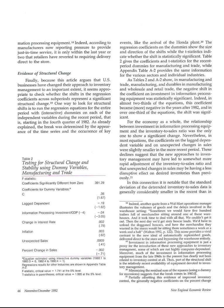
Table 2Testing for Structural Change andStability using Dummy Variables,Manufacturing and TradeF-statistic:Coefficients Significantly Different from Zero 391.29

Coefficients for Dummy Variables:a

C .38(1.67)

Lagged Dependent -.19(-1.62)

Information Processing InvestmentJGDP (-4) -.04(-3.05)

Change in Interest Rate .002(.79)

Inflation .003(.62)

Unexpected Sales .0009(.41)

Percent Change in Sales -.002(-.71)

aEquation estimated using interactive dummy variables (1968:1 to1982:3 = 0, 1982:4 Io 1990:4 = 1)Regressions results |or other industries are shown in Appendix TableA-2.F-statistic, critical value = 1.741 at the 5% level.T-statistics in parentheses; critical value = 1.995 at the 5% level.

events, like the arrival of the Honda plant.2° Theregression coefficients on the dummies show the sizeand direction of the shifts while the t-statistics indi-cate whether the shift is statistically significant. Table2 gives the coefficients and t-statistics for the recent-period dummies for manufacturing and trade, whileAppendix Table A-2 provides the same informationfor the various sectors and individual industries.

As Tables 2 and A-2 show, in manufacturing andtrade, manufacturing, and durables in manufacturingand wholesale and retail trade, the negative shift inthe coefficient on investment in information process-ing equipment was statistically significant. Indeed, inalmost two-thirds of the equations, this coefficientbecame (more) negative in the years after 1982, and inover one-third of the equations, the shift was signif-icant.

For the economy as a whole, the relationshipbetween investment in information processing equip-ment and the inventory-to-sales ratio was the onlyone to show a significant change. Nevertheless, inmost equations, the coefficients on the lagged depen-dent variable and on unexpected changes in saleswere slightly smaller in the more recent period. Thesedeclines suggest that the new approaches to inven-tory management may have led to somewhat morerapid adjustment of the inventory-to-sales ratio andthat unexpected changes in sales may be having a lessdisruptive effect on desired inventories than previ-ously.21

In this connection it is notable that the standarddeviation of the detrended inventory-to-sales data isgenerally considerably smaller in the recent than in

18 Indeed, another quote from a Wal-Mart operations managerillustrates the volumes of goods and the delays involved in thewarehouse setting: "Sometimes we would have five hundredtrailers full of merchandise sitting around one of those ware-houses. And it took time to deal with all that. We couldn’t get itout. Then the next day we’d get sixty boxcar loads. We’d have tounload the doggoned boxcars, and here the merchandise theywanted in the stores would be sitting there sometimes a week or aweek and a half" (Walton 1992, p. 122). This scene provides a vividcontrast to the new ideal of automatically replenished goods,delivered direct to the store and bypassing the warehouse entirely.

19 Investment in information processing equipment is just aproxy for the introduction of these new approaches to inventorymanagment, some of which are not highly computer-dependent.Moreover, much of the investment in information processingequipment from the late 1960s to the present has clearly not beenrelated to inventory control at all. Thus, part of the structural shiftis the relatively recent availability of equipment devoted to inven-tory management.

20 Minimizing the residual sum of the squares (using a dummyfor recessions) suggests that the break comes in 1983:II.

2~ Partially offsetting this evidence of improved inventorycontrol, the generally negative coefficients on the percent change


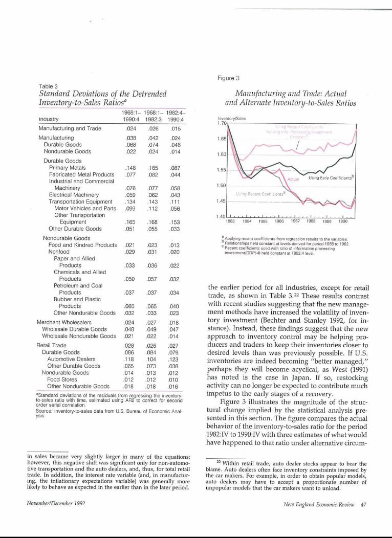
Table 3Standard Deviations of the DetrenfleflInventonj-to-Sales Ratios~

1968:1- 1968:1- 1982:4-Industry 1990:4 1982:3 1990:4Manufacturing and Trade .024 .026 .015Manufacturing .038 .042 .024

Durable Goods .068 .074 .046Nondurable Goods .022 .024 .014Durable Goods

Primary Metals .148 .165 .087Fabricated Metal Products .077 .082 .044Industrial and Commercial

Machinery .076 .077 .058Electrical Machinery .059 .062 .043Transportation Equipment .134 .143 .111

Motor Vehicles and Parts .099 .112 .056Other Transportation

Equipment .165 .168 .153Other Durable Goods .051 .055 .033

Nondurable GoodsFood and Kindred Products .021 .023 .013Nonfood .029 .031 .020

Paper and AlliedProducts .033 .036 .022

Chemicals and AlliedProducts .050 .057 .032

Petroleum and CoalProducts .037 .037 .034

Rubber and PlasticProducts .060 .065 .040

Other Nondurable Goods .032 .033 .023Merchant Wholesalers .024 .027 .018

Wholesale Durable Goods .048 .049 .047Wholesale Nondurable Goods .021 .022 .014

Retail Trade .028 .026 .027Durable Goods .086 .084 .079

Automotive Dealers .118 .104 .123Other Durable Goods .065 .073 .038

Nondurable Goods .014 .013 .012Food Stores .012 .012 .010Other Nondurable Goods .018 .018 .016

aStandard deviations of the residuals from regressing the inventory-to-sales ratio wilh time, estimated using AR2 to correct for secondorder serial correlation.Source: Inventory-to-sales data from U.S. Bureau of Economic Anal-ysis.

in sales became very slightly larger in many of the equations;however, this negative shift was significant only for non-automo-tive transportation and the auto dealers, and, thus, for total retailtrade. In addition, the interest rate variable (and, in manufactur-ing, the inflationary expectations variable) was generally morelikely to behave as expected in the earlier than in the later period.

Figure 3

Manufacturing and Trade: Actualand Alternate Inventory-to-Sales Ratios

Inventon//Sales1.70

1.60

1.5!~~y~ CoeffiCientsb

1.5( ~,,~

1.40 I ~ ~ ~ I ~ ~ ~ I , , , I , , , I , , , I , , , I ~ ~ ~ I ~ ~1983 1984 1985 1986 1987 1988 1989 1990

b Applying recent coefficients from regression resulls to the variablesRelationships held constant at levels derived for pedod 1968 to 1982,

c Recent coefficients used with ratio of informalion processinginvestrnentJGDP(4) held constant at 1982:4 level.

the earlier period for all industries, except for retailtrade, as shown in Table 3.22 These results contrastwith recent studies suggesting that the new manage-ment methods have increased the volatility of inven-tory investment (Bechter and Stanley 1992, for in-stance). Instead, these findings suggest that the newapproach to inventory control may be helping pro-ducers and traders to keep their inventories closer todesired levels than was previously possible. If U.S.inventories are indeed becoming "better managed,"perhaps they will become acyclical, as West (1991)has noted is the case in Japan. If so, restockingactivity can no longer be expected to contribute muchimpetus to the early stages of a recovery.

Figure 3 illustrates the magnitude of the struc-tural change implied by the statistical analysis pre-sented in this section. The figure compares the actualbehavior of the inventory-to-sales ratio for the period1982:IV to 1990:IV with three estimates of what wouldhave happened to that ratio under alternative circum-

22 Within retail trade, auto dealer stocks appear to bear theblame. Auto dealers often face inventory constraints imposed bythe car makers. For example, in order to obtain popular models,auto dealers may have to accept a proportionate number ofunpopular models that the car makers want to unload.

November/December 1992 Nezo England Economic Review 47

stances,a3 The first estimate, derived by applying thecoefficients from the regression results for the recentperiod to the independent variables, merely indicatesthat the estimates follow the actual ratios quiteclosely. A second estimate, using the coefficientsfrom the early period, shows what would have hap-pened to the inventory-to-sales ratio if the relation-ships between variables had remained unchangedfrom those derived for the period from 1968 to 1982.In sharp contrast to its actual behavior, by late 1990the inventory-to-sales ratio would have been ap-proaching its late 1982 peak, if the underlying rela-tionships had not changed. The final estimate, whichuses coefficients from the recent period but does notallow investment in information processing equip-ment as a share of GDP to rise from its 1982:IV level,suggests that this investment mattered. In otherwords, the new approaches to inventory manage-ment represented by this investment appear to belargely responsible for the observed decline in theinventory-to-sales ratio.

Figure 4

Expenditures on PrivateNom’esidential Structures

Billions of 1987 Dollars2O0

160

120

8O

4O

1975 1977 1979 1981 1983 1985 1987 1989 1991

Source: U.S. Bureau of Economic Anal,/s~s

Consequences for the Economy

The previous section presented statistical evi-dence suggesting that the relationship between theinventory-to-sales ratio and its determinants changedsignificantly in the 1980s, and that new approaches toinventory management, proxied by investment ininformation processing equipment, were largely re-sponsible for the change. This section begins toexplore the implications for the economy and thecurrent recovery.

As already mentioned, reducing inventories bothreflects and permits productivity improvements. Ac-cordingly, the evidence of a structural change in therelationship between inventory and sales just pre-sented is good news for the U.S. economy in the longrun. It is even good news for this country’s produc-tivity performance and for corporate profits in theshort run.

Nevertheless, the transition to lean inventorysystems is currently exerting a noticeable drag on theU.S. economy. This drag takes two forms. First, apermanent reduction in the desired inventory-to-sales ratio requires absorbing goods from existingstocks, or, as some commentators put it, making aone-time cut in the length of the pipeline. In addition,lean inventory management permits considerablesavings in space and in workers required to track andhandle stocks. This second source of friction is prob-

ably the more important.To start with the first issue, reducing the length

of the pipeline requires satisfying part of currentdemand from existing stocks without replacing them.For a variety of reasons~but primarily, it seems, theintroduction of new methods of inventory manage-ment--between late 1982 and late 1990, manufactur-ing and trade inventories declined from 1.68 to 1.43months’ sales. In manufacturing the decline was from1.99 to 1.47 months’ sales; in manufacturing dura-bles, from 2.70 to 1.76. Those changes are equivalentto eliminating a week’s worth of sales in manufactur-ing and trade combined or two weeks’ worth ofproduction in manufacturing. In manufactured dura-bles, demand for a month’s worth of output in effectevaporated. Spread over eight years, the evaporationof demand due to inventory reduction was probablynot earthshaking. But such changes certainly must becontributing to the sensation that a frustrating "headwind" is slowing economic growth.

The second source of drag on the U.S. recovery isthe significant savings in space and personnel per-mitted by the new approaches to inventory control.

23 In these dynamic estimates, the lagged dependent variablewas allowed to take the estimated value of the dependent variablein the previous period rather than its actual value.


This second source of friction was not addressed bythe regressions developed for this article, but may,nevertheless, be the more consequential if the sav-ings mentioned in the individual company anecdotesare at all representative.

In those anecdotes, to start with space, a com-pany introducing a JIT or an MRPII inventory systemfrequently emptied one-third of the area formerlydevoted to storing stocks. In addition, these compa-nies found that they needed less space for the pro-duction line and the rework area. These savings mayhelp to explain why industrial structures failed toparticipate fully in the real estate boom of the 1980s,as shown in Figure 4. In addition, David Shulman ofSalomon Brothers has suggested that the next fewyears may witness a glut of warehouse space, in partbecause of the new approaches to inventory manage-ment (Shulman 1991).

Similarly, companies introducing new inventorymanagement systems claim to reap considerable sav-ings in personnel. Manufacturers need fewer peopleto move, track, and order materials and finishedgoods inventories. And, by definition, reducingwork-in-process inventory involves increasing pro-ductivity. Retail firms have also found that they canreduce staffing for handling and managing inventoryas well as clerks for manning the cash registers andmarking and remarking merchandise. Accordingly,adoption of the new inventory management systemshas undoubtedly contributed to the recent declines inmanufacturing and retail employment. Firms’ abilityto "downsize" and "rightsize" may be partly attrib-utable to their adopting new inventory managementsystems. Moreover, these changes are secular, notcyclical. As many observers have noted, "These jobsaren’t coming back again."

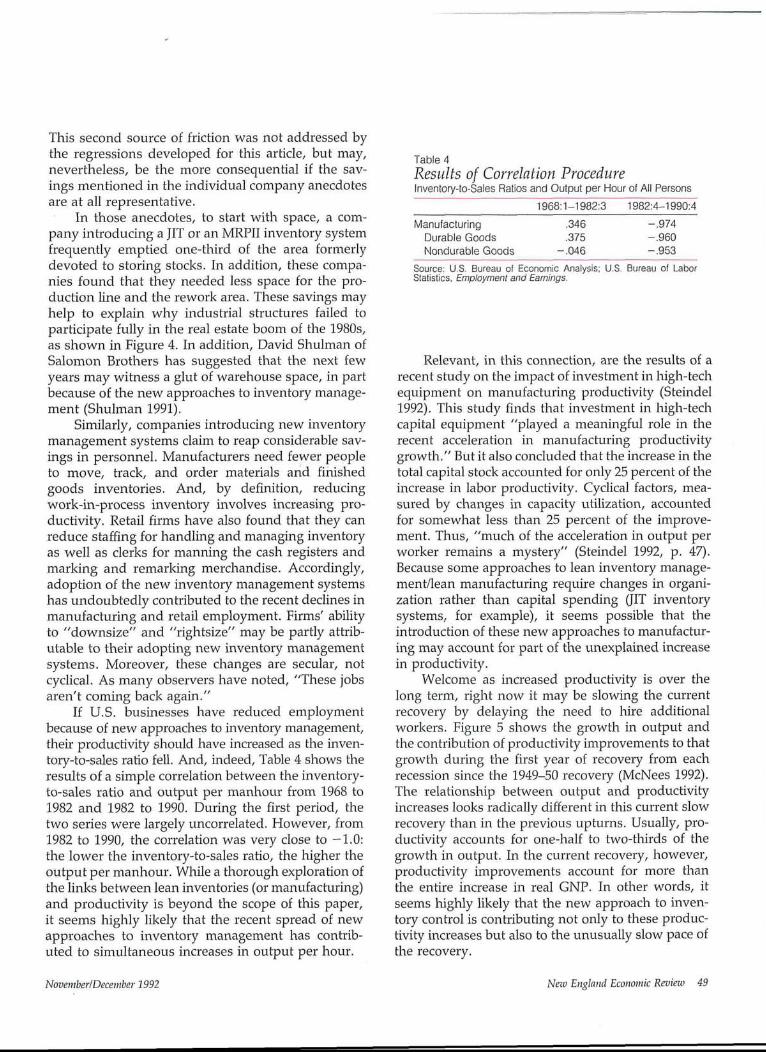
If U.S. businesses have reduced employmentbecause of new approaches to inventory management,their productivity should have increased as the inven-tory-to-sales ratio fell. And, indeed, Table 4 shows theresults of a simple correlation between the inventory-to-sales ratio and output per manhour from 1968 to1982 and 1982 to 1990. During the first period, thetwo series were largely uncorrelated. However, from1982 to 1990, the correlation was very close to -1.0:the lower the inventory-to-sales ratio, the higher theoutput per manhour. While a thorough exploration ofthe links between lean inventories (or manufacturing)and productivity is beyond the scope of this paper,it seems highly likely that the recent spread of newapproaches to inventory management has contrib-uted to simultaneous increases in output per hour.

Table 4Results of Correlation ProcedureInventory-to-Sales Ratios and Output per Hour of All Persons

1968:1-1982:3 1982:4-1990:4Manufacturing .346 -.974

Durable Goods .375 -.960Nondurable Goods -.046 -.953

Source: U.S. Bureau o! Economic Analysis; U.S. Bureau of LaborStatistics, Employment and Earnings.

Relevant, in this connection, are the results of arecent study on the impact of investment in high-techequipment on manufacturing productivity (Steindel1992). This study finds that investment in high-techcapital equipment "played a meaningful role in therecent acceleration in manufacturing productivitygrowth." But it also concluded that the increase in thetotal capital stock accounted for only 25 percent of theincrease in labor productivity. Cyclical factors, mea-sured by changes in capacity utilization, accountedfor somewhat less than 25 percent of the improve-ment. Thus, "much of the acceleration in output perworker remains a mystery" (Steindel 1992, p. 47).Because some approaches to lean inventory manage-ment/lean manufacturing require changes in organi-zation rather than capital spending (JIT inventorysystems, for example), it seems possible that theintroduction of these new approaches to manufactur-ing may account for part of the unexplained increasein productivity.

Welcome as increased productivity is over thelong term, right now it may be slowing the currentrecovery by delaying the need to hire additionalworkers. Figure 5 shows the growth in output andthe contribution of productivity improvements to thatgrowth during the first year of recovery from eachrecession since the 1949-50 recovery (McNees 1992).The relationship between output and productivityincreases looks radically different in this current slowrecovery than in the previous upturns. Usually, pro-ductivity accounts for one-half to two-thirds of thegrowth in output. In the current recovery, however,productivity improvements account for more thanthe entire increase in real GNP. In other words, itseems highly likely that the new approach to inven-tory control is contributing not only to these produc-tivity increases but also to the unusually slow pace ofthe recovery.


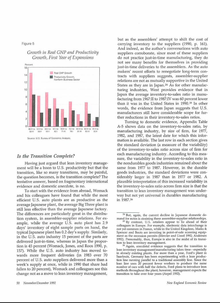
Figure 5

Growth in Real GNP and ProductivityGrowth, First Year of Expansions

Percent16

Real GNP Growth14

¯ Productivit~ Growth,Nonfarm Business Sec’[or

12

10

50 IV 55:11 59:11 621 7r:IV 761 8] III 83:1V 9211

Source: U.S. Bureau of Economic Analysis

Is the Transition Complete?Having just argued that lean inventory manage-

ment will be a boon to U.S. productivity but that thetransition, like so many transitions, may be painful,the question becomes, is the transition complete? Thetentative answer, based on fragmentary internationalevidence and domestic anecdote, is no.

To start with the evidence from abroad, Womackand his colleagues have found that while the mostefficient U.S. auto plants are as productive as theaverage Japanese plant, the average Big Three plant isstill less effective than the average Japanese factory.The differences are particularly great in the distribu-tion system, in assembler-supplier relations. For ex-ample, while the average U.S. auto plant has 2.9days’ inventory of eight sample parts on hand, thetypical Japanese plant has 0.2 day’s supply. Similarly,in the U.S. auto industry 15 percent of the parts aredelivered just-in-time, whereas in Japan the propor-tion is 45 percent (Womack, Jones, and Roos 1990, p.157). While the U.S. auto industry has moved to-wards more frequent deliveries (in 1983 over 70percent of U.S. auto suppliers delivered more than aweek’s supply at once, while in 1990 that share hadfallen to 20 percent), Womack and colleagues see thischange not as a move to lean inventory management,

but as the assemblers’ attempt to shift the cost ofcarrying inventory to the suppliers (1990, p. 161).And indeed, as the author’s conversations with autosuppliers corroborate, since most of these suppliersdo not practice just-in-time manufacturing, they donot see many benefits for themselves in providingjust-in-time deliveries to the assemblers. As the automakers’ recent efforts to renegotiate long-term con-tracts with suppliers suggests, assembler-supplierrelations are not as mutually supportive in the UnitedStates as they are in Japan.24 As for other manufac-turing industries, West provides evidence that inJapan the average inventory-to-sales ratio in manu-facturing from 1967:II to 1987:IV was 60 percent lowerthan it was in the United States in 1990.25 In otherwords, the evidence from Japan suggests that U.S.manufacturers still have considerable scope for fur-ther reductions in their inventory-to-sales ratios.

Turning to domestic evidence, Appendix TableA-5 shows data on the inventory-to-sales ratio, bymanufacturing industry, by size of firm, for 1977,1982, and 1987, the latest date for which this infor-mation is available. The last row in each section givesthe standard deviation (a measure of the variability)of the inventory-to-sales ratio across size of firm foreach manufacturing industry. According to this mea-sure, the variability in the inventory-to-sales ratio inthe nondurables goods industries remained about thesame from 1977 to 1987. However, in the durablegoods industries, the standard deviations were con-siderably larger in 1987 than in 1977 or 1982. Aplausible interpretation of this increased variability inthe inventory-to-sales ratio across firm size is that thetransition to lean inventory management was under-way but not yet universal in durables manufacturingin 1987.26

24 But, again, the current decline in Japanese domestic de-mand for autos is straining these assembler-supplier relationships.

25 By contrast, U.S. retailers appear to be ahead of theircolleagues in Europe. For example, electronic data interchange isnot yet common in France, while in the United Kingdom, Marks &Spencer and Boots are investing in point-of-sale scanning equip-ment as the recession permits (Mercier and Uzeel 1992; Andersen1992). Presumably, thus, Europe is also in the midst of its transi-tion to lean inventory management.

26 Again, anecdotal evidence suggests that the transition tolean inventory management/manufacturing takes time--especiallyin already existing plants. For more than a year, Ford’s plant inSaarlouis, Germany has been experimenting with a lean produc-tion line running parallel to a traditional assembly line. Since thelean line uses 20 percent fewer workers to produce the samenumber of cars with half the defects, Ford plans to introduce leanmethods throughout the plant; however, management expects thetransition to take over four years (Aepel 1992).


More currently, anecdotal evidence suggests thatthe transition continues. U.S. manufacturers whoswitched to new inventory management systemssome time ago indicate that they believe they candrive inventories down even further, that the opti-mum inventory-to-sales ratio has not yet beenreached. They also report that their own company isahead of its industry in its attention to inventorycontrol. Press coverage of companies like Colt,F.A.Oo Schwarz, and Home Depot indicates thatmany well-known firms are still making the transitionto new inventory control programs. For instance, inmid 1992 Home Depot was just implementing anelectronic data interchange purchasing program link-ing the company’s inventory system with major ven-dors. Similarly, at Colt, which filed for Chapter 11bankruptcy protection in March 1992, the new chiefexecutive officer hired to turn the company around isplanning to streamline the manufacturing processthrough just-in-time inventory control and othertechniques that, he indicates, will require minimalcapital investment (Bryant 1992).

Altogether, this scattered empirical and anec-dotal evidence suggests that the move to inventoryreduction is not yet complete. As a consequence, thetransition to lean inventory management is likely tocontinue to slow the pace of U.S. economic growthfor some time to come.

Conclusion

This article has presented evidence to suggestthat the introduction of new approaches to inventorymanagement represents a structural change for theU.S. economy. Moreover, while learning to live withlean inventories saves resources and will ultimatelyimprove U.S. economic welfare unambiguously, theongoing transition is slowing the recovery. In otherwords, the frequently recited list of structural issuesoverhanging the economy--the excessive debt bur-dens, the overbuilding in commercial real estate, andthe demographic shifts--should be expanded to in-clude the introduction of the new inventory systems.A focus on these new systems helps to explainseveral puzzling characteristics of the current recalci-tant recovery: why, for instance, "these jobs reallyaren’t coming back again;" why the anticipated re-building of unusually lean inventories did notreignite the economy; and why corporate profits andproductivity improvements have been surprisinglygood. Finally, these structural changes also suggestthat policymakers probably have scope for morestimulative action than would have been appropriatein previous recoveries.

Appendix

Table A-1Regression Results

Info Process. Change in PercentLagged Investment/ Interest Unexpected Change in

Industry C Dependent GDP (-4) Rate Inflation Sales Salesa

Total Manufacturing1968:1-1982:3 0.34 0.80 -0.001700 -0.003593 0,004162 -0.007412 -0.017

(8.88) (34.39) (-0.28) (-2.95) (3.95) (- 11.59) (- 12.47)1982:4-1990:4 0,51 0.74 -0.046733 -0.001593 0.013510 -0.005793 -0.015

(3.51) (12.56) (-3.94) (-0.49) (2.81) (-4.12) (-4.61)1968:1-1990:4 0,26 0.86 -0.012291 -0.002874 0,003630 -0.007383 -0,016

(6.42) (37.84) (-5,05) (-2.51) (3.17) (-13.74) (-10.57)

Durable Goods1968:1-1982:3 0,45 0.77 0.031370 -0.006257 0.004642 -0.007969 -0.023

(10.16) (33,45) (2.86) (-3.49) (2.86) (-12.47) (-14.31)1982:4-1990:4 0.82 0.71 -0.091404 -0.001943 0.019152 -0.007348 -0.024

(6.16) (18.67) (-6.80) (-0.50) (3,93) (-5.60) (-8,31)1968:1-1990:4 0.77 0.68 -0.045666 -0.004050 0,004280 -0.006739 -0.028

(7.04) (16.07) (-3.04) (-3.05) (1.51) (-11.94) (-16.09)

Durbin Adj.Rho~ Watson R2

0.00(0.00) 1.93 0,989

0.00(0.00) 1.74 0.995

0.40(3.70) 1.94 0,980

0.10(0.67) 1.96 0.991

-0.20(-0.99) 1.72 0.998

0.90(19.80) 2.30 0.931

(Continued)


Table A-1 continued (2)Regression Results

Industry CNondurable Goods

1968:1-1982:3 0.13 0.91(2.20) (20.31)

1982:4-1990:4 0.29 0.78(1.93) (8.11)

1968:1-1990:4 0.18 0.86(3.98) (25.02)

Info Process. Change in PercentLagged Investment/ Interest Unexpec[ed Change in Durbin Adj.

Dependent GDP (-4) Rate Inflation Sales Sales" Rhob Watson R2

-0.020929 -0.001896 0.003507 -0.008739 -0.008(-3.78) (-1.65) (3.40) (-8.90) (-4.84)

-0.019755 -0.000571 0.008278 -0.002573 -0.007(-2.18) (-0.18) (1.69) (-1.55) (-2.00)

-0.009223 -0,002178 0.001988 -0.006992 -0.009(-4.39) (- 1.92) (2.79) (-8.04) (-5.64)

2.25 0.930

1.89 0.976

1,85 0.977

Wholesale1968:1-1982:3 0.94 0.31

(5.39) (2.37)1982:4-1990:4 0.76 0.46

(2.64) (2.46)1968:1-1990:4 0.96 0.32

(6.78) (3.11)

0.021473 -0.001181 -0.004580 -0.001602(0.90) (-0.99) (-1.81) (-1.65)

-0.013335 0.000053 0.001590 -0.000132(-1.87) (0.01) (0.21) (-0.06)

-0.010422 -0.001081 -0.002987 -0.001461(-1.62) (-1.02) (-1.48) (-1.82)

-0.018 0.80(-7.42) (8.37) 2.08 0.658

-0.018 0.30(-3.55) (1.00) 1.88 0.771

-0.018 0.80(-8.91) (10.38) 2.10 0.636

Wholesale Durable Goods1968:1-1982:3 0.19 0.92

(3.00) (27.85)1982:4-1990:4 0.81 0.64

(4.69) (9.54)1968:1-1990:4 0.24 0.89

(4.87) (36.64)

0.014038 -0.003215 -0.002296 -0.008704 -0.018(1.21) (-1.55) (-1.23) (-7.97) (-10.26)

-0.040051 0.000531 0.003727 -0.006267 -0.022(-3.43) (0.08) (0.39) (-2.18) (-5.35)

-0.006456 -0,002858 0.001062 -0.008850 -0.017(-2.64) (-1.27) (0.82) (-7.97) (-10.17)

1,88 0.975

2.24 0.956

1.73 0.962

Wholesale Nondurable Goods1968:1-1982:3 0.99 -0.09

(7.09) (-0.62)1982:4-1990:4 0.58 0.32

(2.51) (1.16)1968:1-1990:4 0.88 -0.01

(8.98) (-0.12)

-0.045842 -0.000605 -0.001986 0.000712(-1.09) (-0.47) (-0.69) (1.01)

0.007623 0.000670 -0.004244 -0.000486(0.84) (0.21) (-0.59) (-0.47)

-0.002313 -0.000415 -0.003203 0.000531(-0.20) (-0.39) (-1.40) (1.00)

-0.012 O.9O(-5.52) (13.66) 1.74 0.344-0.011 0.60(-3.61) (2.37) 2.02 0.429-0,012 0.90(-7.16) (18.57) 1.81 0.370

Retail1968:1-1982:3 0.38 0.75

(3.80) (10.52)1982:4-1990:4 0.76 0.51

(3.30) (2.74)1968:1-1990:4 0.51 0.66

(5.62) (9.96)

0.014094 -0.002079 -0.004057 -0.005152 -0,014(1.74) (-1.35) (-2.81) (-4.32) (-5.08)

0.006666 0.008902 -0.006671 -0.001548 -0.032(0.43) (1.70) (-0.86) (-0.60) (-4.34)

0.009023 -0.000358 -0.003508 -0.004638 -0,018(2.96) (-0.23) (-3.39) (-4.07) (-6.73)

2.29 0.845

1.61 0.887

1.96 0.896

Retail Durable Goods1968:1-1982:3 0.67 0.68

(4.15) (8.02)1982:4-1990:4 1.21 0.54

(6.07) (5.32)1968:1-1990:4 0.75 0.65

(5.75) (9.51)

0.015944 -0.008464 -0.001405 -0.006549 -0.016(0.63) (-1.72) (-0.29) (-4.84) (-4.47)

-0.045841 0.015477 -0.021928 -0.003331 -0.044(-3.29) (1.60) (-1.58) (-1.71) (-7.95)

-0.013733 -0.003049 0.000619 -0.006254 -0.021(-2.68) (-0.69) (0.19) (-5.29) (-7.07)

2.47 0.812

2.16 0.795

2.21 0.817

Retail Nondurable Goods1968:1-1982:3 0.32 0.74

(4.51) (12,52)1982:4-1990:4 0.20 0.84

(1.64) (6.83)1968:1-1990:4 0.26 0.79

(5.31) (I8.50)

0.000815 -0.002156 -0.003472 -0.002262 -0.014(0.15) (-2.32) (-4.41) (-1.55) (-5.75)

-0.000205 0.003034 0.001794 -0.003647 -0.018(-0.03) (1.19) (0.38) (-1.48) (-2.52)

0.005024 -0.001599 -0.003663 -0.003186 -0.014(3.17) (-1.86) (-5.81) (-2.62) (-6.34)

1.51 0.859

2.06 O.934

1.59 0.957



Info Process. Change in PercentLagged Investment/ Interest Unexpected Change Durbin Adj.

Industry C Dependent GDP (-4) Rate Inflation Sales in Salesa Rhob Watson R2Manufacturing Durable GoodsPrimary Metals

1968:1-1982:3 0.09 0.97 -0.048128 -0.011311 0.006840 -0.010175 -0.026 -0.10(1.92) (36.02) (-1.57) (-2.29) (1.87) (-11.49) (-14.36) (-0.68) 1.99 0.986

1982:4-1990:4 -0.05 0.88 -0.011734 0.011522 0.076152 -0.010194 -0.017 -0,20(-0.48) (31.18) (-0.88) (1.25) (6.77) (-6.61) (-6.62) (- 1.03) 1.89 0.995

1968:1-1990:4 0.20 0.89 -0.005912 -0.006773 0.007561 -0.009155 -0.027 0.30(-0.86) (-1.53) (2.25) (-13.46) (-13.60) (2.73) 2.11 0.967(3.79) (41.14)

Fabricated Metals1968:1-1982:3 0.46 0.75

(3.14) (8.86)1982:4-1990:4 0.94 0.66

(2.62) (5.53)1968:1-1990:4 0.35 0.83

(3.80) (17.65)Industrial & Commercial Machinery1968:1-1982:3 1.60 0.43

(8.73) (7.34)

0.027292 0.000417 0.005264 -0.006845 -0.028 0.60(0.65) (0.12) (0.88) (-5.66) (- 7.68) (4.41) 2.09 0.884

-0.058109 0.001101 -0.017131 -0.005644 -0.025 0.00(-2.56) (0.16) (-1.27) (-3.48) (-4.85) (0.00) 1.92 0.976

-0.008597 -0.000782 0.004754 -0.007212 -0.025 0.50(-1.29) (-0.26) (1.29) (-8.64) (-9.49) (4.60) 2.15 0.912

0.016601 -0.002164 0.010134 -0.005125 -0.043 0.90(0.31) (-1.41) (2.96) (-4.77) (-13.37) (24.48) 2.38 0.934

1982:4-1990:4 0.51 0.83 -0.104470 -0.003654 0.035510 -0.008045 -0.022 0.40(2.38) (19.08) (-3.10) (-0.58) (2.88) (-6.02) (-6.69) (2.08) 1.75 0,995

1968:1-1990:4 1.00 0.69 -0.129000 -0.002279 0.013830 -0.008085 -0.030 0.90(5.97) (15.25) (-4.82) (-1.24) (3.51) (-9.07) (-11.52) (22.31) 2.40 0.932

Electronic Machinery1968:1-1982:3 1.13 0.49 0.046047 -0.004036 0.006673 -0.004219 -0.027 0.70

(5.90) (5.61) (1.46) (-1.94) (1.52) (-3.49) (-9.62) (5.78) 2.05 0.8701982:4-1990:4 0.93 0.69 -0.088875 -0.005720 0.018048 -0.005978 -0.026 0.60

(2.04) (4.73)1968:1-1990:4 1.34 0.47

(6.87) (6.21)Motor Vehicles & Parts

1968:1-1982:3 0.26 0.80(3.94) (11.71)

1982:4-1990:4 0.24 0.77(1.90) (6.86)

1968:1-1990:4 0.29(5.29) (13.98)

Other Transportation1968:1-1982:3 0.64 0.81

(2.96) (14.46)1982:4-1990:4 0.37 0.91

(0.96) (10.98)1968:1-1990:4 0,20 0.94

(1.34) (25.91)Other Durable Goods1968:1-1982:3 0.46 0.75

(3.77) (10.47)1982:4-1990:4 0.7I 0.70

(2.47) (6.49)1968:1-1990:4 0.34 0.83

(4.47) (20.24)

(-2.83) (-0.86) (1.11) (-2.93) (-4.16) (3.90) 2.24 0.888-0.055348 -0.004059 0.003711 -0.004021 -0.028 0.90

(-2.55) (-2.33) (0.92) (-4.21) (-12.41) (18.07) 2.10 0.826

-0.046658 -0.007147 0.000125 -0.003901 -0.011(-2.07) (-1.80) (0.03) (-8.41) (-9.61)

-0.028008 0.000101 0.006864 -0.002448 -0.009(-2.54) (0.01) (0.65) (-4.46) (-6.09)

0.77 -0.029661 -0.006711 -0.001237 -0.003454 -0.011(-4.43) (-2.02) (-0.50) (-9.52) (-12.04)

0.104010 0.003648 -0.006163 -0.014497 -0.038(2.48) (0.47) (-0.92) (-6.94) (-6.39)

-0.024926 -0.020543 0.042378 -0.015601 -0.074(-0.93) (-0.98) (1.29) (-4.56) (-6.09)

0.023994 0.007954 0.004672 -0.016980 -0.034(2.24) (1.00) (1.03) (-9.11) (-6.93)

2.12 0.881

1.72 0.877

2.15 O.95O

1.71 0.929

1.76 0.919

1.68 O.943

0.017132 -0.003573 0.004159 -0.007245 -0.019 0.50(0.78) (-1.71) (1.36) (-7.60) (-6.58) (3.43) 1.80 0.930

-0.053795 -0.000467 0.004005 -0.004878 -0.021 0.40(-2.55) (-0.08) (0.37) (-3.43) -4.03) (1.70) 1.83 0.948

-0.014073 -0.002953 0.004234 -0.007389 -0.018 0.50(-3.11) (-1.55) (1.88) (-10.49) (-7.75) (4.63) 1.91 0.934

aPolynomial Distributed Lag (first degree polynomial, 3 quarters including current quarter, far endpoint constraint).bEstimated using the Hildreth-Lu method for correcting first order serial correlation.Coefficients shown are the sum of the estimated lagged coefficients.T-statistics in parentheses; critical value = 1.993 at the 5% level.


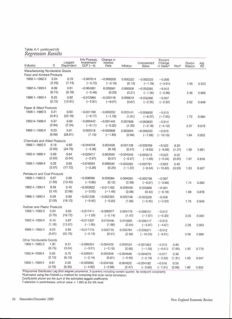
Table A-1 continued (4)

Regression ResultsInfo Process, Change in Percent

Lagged Investment/ Interest Unexpected Change Durbin Adj.Industry C Dependent GDP (-4) Rate Inflation Sales in Salesa Rhou Watson R2Manufacturing Nondurable GoodsFood and Kindred Products

1968:1-1982:3 0.24 0.78 -0.007914 -0.000208 0.000222 -0.002233 -0.006(2.23) (7.74) (-0.72) (-0.10) (0.13) (-1.78) (-2.01) 1.95 0.523

1982:4-1990:4 0.09 0.91 -0.004091 0.000561 0.000936 -0.003285 -0,012(0.74) (8.78) (-0.46) (0.20) (0.21) (-1.35) (-2.98) 2.36 0.966

1968:1-1990:4 0.20 0.82 -0.012965 -0,000116 0,000810 -0.002366 -0,007(2.72) (12.01) (-2.81) (-0.07) (0.87) (-2.35) (-2,92) 2.02 0.949

Paper & Allied Products1968:1-1982:3 0.21 0.83 -0.001799 -0.003252 0.003141 -0.006836 -0,015

(4.91) (22.19) (-0.17) (-1,78) (1.81) (-6.37) (-7.95) 1.73 0.9641982:4-1990:4 0.37 0.69 -0.000442 -0.001445 0.007898 -0.003830 -0,014

(2,94) (7,24) (-0,11) (-0.32) (1.30) (-2.18) (-4.12) 2.37 0.8181966:1-1990:4 0.23 0.81 0.002218 -0.002909 0.003004 -0.006233 -0.015

(6.50) (26.61) (1.15) (-1.83) (2.84) (-7.08) (-10.15) 1.84 0.955

Chemicals and Allied Products1968:1-1982:3 0.18 0.93 -0.044018 0.000439 0.001128 -0.009769 -0.022 0.20

(2.63) (24.75) (-3.36) (0.19) (0.47) (-9.59) (-9.68) (1.37) 1.92 0.9511982:4-1990:4 0.69 0.64 -0.029417 0.003590 -0.004240 -0.003515 -0.023 0.20

(2.62) (5.04) (-2.67) (0.57) (-0.37) (- 1.68) (-5.04) (0.85) 1.97 0.9181968:1-1990:4 0.32 0.85 -0.016584 0.000540 -0.002583 -0.007791 -0.023 0.40

(3.57) (17.72) (-3.28) (0.25) (- 1.32) (-8.54) (- 10.65) (3.53) 1.93 0.927

Petroleum and Coal Products1968:1-1982:3 0.07 0.89 -0.008596 0.000264 0.004090 -0,005736 -0.007

(1.50) (13.45) (-0.65) (0.12) (2.39) (-6.07) (-3.96) 1.74 0.8821982:4-1990:4 0,59 0.40 -0.062622 -0,011182 0.026458 0,000668 -0.001

(3.19) (2.56) (-3.55) (-1.49) (2.09) (0.42) (-0.19) 1.89 0.8781968:1-1990:4 0.08 0.89 -0.001338 -0.002365 0.002746 -0.003206 -0,006

(2.08) (19.13) (-0.45) (-0.90) (1.96) (-3.45) (-3.03) 1.79 0.840

Rubber and Plastic Products1968:1-1982:3 0.24 0.85 -0.017411 -0.000377 0.004779 -0.006151 -0.012

(3.75) (16.72) (-1.08) {-0.14) (1,42) (-7.67) (-6.30) 2,05 0,9601982:4-1990:4 0.15 0.87 -0.011337 0.010446 0.015695 -0.006117 -0.013

(1.18) (13.07) (-1.05) (1,96) (2.04) (-5.97) (-4.67) 2,26 0,9631968:1-1990:4 0.25 0.84 -0.017175 0,000710 0.005704 -0.006071 -0.012

(5.81) (25.75) (-5.13) (0.31) (2.56) (-10,20) (-8.91) 2.06 0.980

Other Nondurable Goods1968:1-1982:3 1,30 0.31 -0.086354 -0,004426 0,008524 -0.001983 -0.019 0.80

(6.75) (3.04) (-3,01) (-3.16) (2.66) (-1,58) (-6.61) (7.86) 1.80 0.770

1982:4-1990:4 0,53 0.75 -0.038241 0.003349 -0,004848 -0.004679 -0.017 0.30(2.15) (6.10) (-2.14) (0.61) (-0.49) (-2.19) (-3.52) (1.31) 1,99 0,947

1968:1-1990:4 0,81 0.58 -0.055932 -0.004105 0.004832 -0.004192 -0.016 0.50(4.70) (6.30) (-4,82) (-2.69) (2.47) (-3.60) (-7.01) (3.86) 1.90 0.955

aPolynomial Distribuled Lag (first degree polynomial, 3 quaders including currenl quarter, far endpoinl constraint).bEstimated using the Hildreth-Lu method for correcting lirst order serial correlation,Coefficients shown are the sum of the eslimated lagged coefficients.T-statistics in parentheses; critical value = 1.993 at the 5% level.



LaggedIndustry C DependentRetail Durable GoodsAuto Dealers

1968:1-1982:3 0.70 0.55(4.41) (5.09)

1982:4-1990:4 0.92 0.59(5.04) (4.61)

1968:1-1990:4 0.67 0.59(5.71) (7.48)

Retail Other Durable Goods1968:1-1982:3 0.52 0.84

(3.76) (16.56)1982:4-1990:4 0.90 0.69

(3.33} (7.96)1968:1-1990:4 0.478 0.86

(4.25) (21.39)Retail Nondurable GoodsFood Stores1968:1-1982:3 0.18 0.71 0.012177

(4.13) (10.16) (2.33)1982:4-1990:4 0.23 0.61 0.022623

(1.79) (2.97) (2.10)1968:1-1990:4 0.20 0.68 0.017748

(4.73) (9.94) (4.82)Retail Other Nondurable Goods1968:1-1982:3 0.35 0.78 -0.006907

(2.38) (7.71) (-0.55)1982:4-1990:4 0.88 0.33 0.003624

(2.88) (1.52) (0.38)1968:1-1990:4 0.32 0.79 0.000053

(3.45) (12.17) (0.02)

Info Process.Inveslment/GDP (-4)

Change inInterest

Rate InflationUnexpected

Sales

PercentChangein Salesa

0.013873 -0.006499 0.008659 -0.004786 -0.01(0.37) (-0.92) (1.15) (-3.80) (-2.70)

-0.004200 0.024676 -0.034246 -0.004571 -0.04(-0.13) (1.54) (-1.44) (-2.10) (-6.90)

0.011095 0.003763 0.003499 -0.004768 -0.02(1.21) (0.55) (0.72) (-4.06) (-5.54)

-0.002642 -0.007868 -0.009278 -0.011009 -0.03(-0.17) (-2.40) (-3.25) (-7.09) (-8.29)

-0.065266 -0.004959 0.010898 -0.008657 -0.02(-3.31) (-0.68) (0.98) (-2.75) (-2.90)

-0.028039 -0.008111 -0.004978 -0.011428 -0.02(-4.60) (-2.80) (-2.66) (-8.55) (-8.83)

-0.000799 0.000108 -0.002361 -0.01(-1.05) (0.18) (-3.24) (-5.98)

-0.003423 0.001422 -0.000436 -0.00(-1.43) (0.36) (-0.31) (-0.27)

-0.001252 -0.000457 -0.001767 -0.01(-1.63) (-1.13) (-2.66) (-5.54)

-0.003193 -0.004504 -0.002065 -0.01(-2.33) (-2.83) (-1.19) (-3.45)

-0.000758 0.013149 -0.002740 -0.02(-0.23) (1.88) (-1.14) (-2.87)

-0.002424 -0.005001 -0.003448 -0.01(-1.97) (-3.87) (-2.51) (-4.27)

Rho~ Durbin Adj.Watson R2

2.37 0.728

2.19 0.874

2.19 0.734

1.77 0.902

2.19 0.959

1.81 0.970

1.96 0.908

2.39 0.943

2.10 0.981

0.30(1.60) 2.07 0.8240.60

(3.79) 2.36 0.6170.30

(2.29) 2.07 0.837

Memo:Inventory Regressions Variable ListVariableDependent Variable:

Inventory-to-Sales RatioIndependent Variables:

Lagged Dependent:Inventory/Sales (- 1)Information Processing Investment (-4)/

Gross Domestic ProductChange in the Interest Ratea

Units

Ratio, Based on 1982 Dollars

Ratio, Based on 1982 Dollars

Ratio, Based on 1982 DollarsPercentage Points

Source

U.S. Bureau of Economic Analysis

U.S. Bureau of Economic Analysis

U.S. Bureau of Economic AnalysisBoard of Governors of the Federal

Change in the Inflation Rateb

Unexpected SalescPercentPercentage Points

Percent Change in Sales’~ Percent

aDiflerence between current quarter and previous quarter, 3-month CD Rate.bpercent change in CPI (less foods and fuels) from a year ago (CORE inflation).CDifference in the percent change from that of the previous quarter.dPercent change in sales from previous quarter.

Reserve SystemU.S. Bureau of Labor StatisticsSales data from U.S. Bureau of

Economic AnalysisSales data from U.S. Bureau of

Economic Analysis


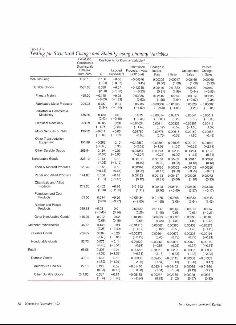
Table A-2Testing for Structural Change and Stability using Dulnmy Variables

Manufacturing

Durable Goods

Primary Metals

Fabricated Metal Products

Industrial & CommercialMachinery

Electrical Machinery

Motor Vehicles & Parts

Other TransportationEquipment

Other Durable Goods

Nondurable Goods

Food & Kindred Products

Paper and Allied Products

Chemicals and AlliedProducts

Pelroleum and CoalProducts

Rubber and PlasticProducts

Other Nondurable Goods

Merchant Wholesalers

Durable Goods

Nondurable Goods

Retail

Durable Goods

Automotive Dealers

Other Durable Goods

F-slatistic:CoefficientsSigniticanlly

Differentfrom Zero

1166.10

1535,00

499.30

204.23

1635,80

203.89

136.32

151.89

269.94

338.10

123.42

144.05

243.20

55.60

335.88

485.29

46.77

228.05

32.73

66.95

39.19

27.13

244.06

Coefficients for Dummy Variable:a

Information Change inLagged Process. Invest./ Interest

C Dependent GDP (-4) Rate0.186 -0.06 -0.04576 0.00205(1.24) (-0.97) (-3.45) (0.60)

0.388 -0.07 -0.12348 0.00440(2.20) (-1.30) (-6.23) (0.91)

-0.115 -0.09 0.03336 0.02145(-0.63) (-1.83) (0.92) (1.55)

0.737 -0.24 -0.05586 -0.00086(1.54) (- 1.44) (- 1.52) (-0.08)

PercentUnexpecled Change

Inflation Sales in Sales

0.00917 0.00165 0.00060(1.88) (1.08) (0.33)

0.01322 0.00067 -0.00107(1.98) (0.44) (-0.55)

0.06654 -0.00014 0.00535(3.64) (-0.07) (2.38)

-0.01963 0.00326 -0.00002(-1.03) (1.21) (-0.01)

0.120 -0.01 -0.11824 -0.00014(0.42) (-0.18) (-2.35) (-0.01)

-0.605 0.28 -0.04034 0.00111(-1.75) (2.54) (-1.62) (0.12)-0.011 -0.03 0.01750 0.00775(-0.06) (-0.18) (0.68) (0.70)

0.03177 0.00641 -0.00017(2.26) (2.16) (-0.06)

0.00823 -0.00357 0.00411(0.57) (- 1.30) (1.37)

0.00616 0.00150 0.00057(0.39) (1.65) (0.48)

-0,268 0.10 -0.12860 -0.02509(-0.60) (0.95) (-2.59) (-1.09)

0,197 -0.06 -0.04354 0.00241(0.87) (-0.60) (-2.07) (0.33)

0,164 -0.13 0.00106 0.00134(1.02) ( - 1.19) (0.10) (0.39)

-0,146 0.13 0.00376 0.00086(-0.64) (0.66) (0.22) (0.17)

0.158 -0.13 0.00133 0.00173(1.01) (-1.13) (0.12) (0.31)

0.04806 -0.00100 -0.01869(1.38) (-0.25) (-2.71)

0.00205 0.00264 0.00123(0.20) (1.18) (0.51)

0.00469 0.00617 0.00036(0.93) (3.18) (0. ! 8)

0.00062 -0.00103 -0.00280(0.08) (-0.25) (-0.81)

0.00487 0.00299 0.00073(0.66) (1.30) (0.33)

0.462 -0.26 0.01593(1.98) (-2.30) (1.11 )

0.00498 -0.00414 0.00635 -0.00038(0.70) (-0.40) (2.57) (-0.17)

0.514 -0.50 -0.05434(3.09) (-3.27) (-2.60)

-0.01165 0.02308 0.00630 0.00348(- 1.68) (2.08) (3.64) (1.45)

-0.081 0.01 0.00522(-0.45) (0.14) (0.25)

0.012 0.02 0.01199(0.06) (0.15) (0.66)

0.448 -0.33 -0.01110(2.28) (-2.49) (- 1.17)

0.587 -0.26 -0.05276(3.60) (-3.81) (-3.29)

0.076 -0.11 0.01020(0.40) (-0.51) (0.91)

0.393 -0.25 -0.00556(1.63) (-1.32) (-0.34)

0.565 -0.16 -0.06000(1.89) (-1.01) (-2.06)

0.242 0.02 -0.01410(0.93) (0.12) (-0.28)

0.367 -0.14 -0.06188(1.06) (-1.26) (-2.24)

0.01117 0.01064 0.00010 -0.00057(1.45) (0.98) (0.06) (-0.27)

0.00900 -0.00896 0.00293 -0.00105(1.58) (-1.03) (1.00) (-0.45)

0.00007 0.00380 0.00439 -0.00273(0.02) (0.58) (1.45) (-1.26)

0.00304 0.00672 0.00225 -0.00191(0.45) (0.73) (0.77) (-0.91)

-0.00257 0.00016 0.00070 -0.00149(-0.58) (0.02) (0.37) (-0.74)

0.01118 -0.00237 0.00357 -0.00808(2.17) (-0.32) (1.32) (-2.22)

0.02456 -0.02115 0.00338 -0.01365(1.84) (-1.13) (1.20) (-3.47)

0.03241 -0.04402 0.00038 -0.01560(1.64) (-1.54) (0.13) (-3.97)

0.00267 0.02056 0.00229 0.00361(0.29) (1.52) (0.57) (0.83)


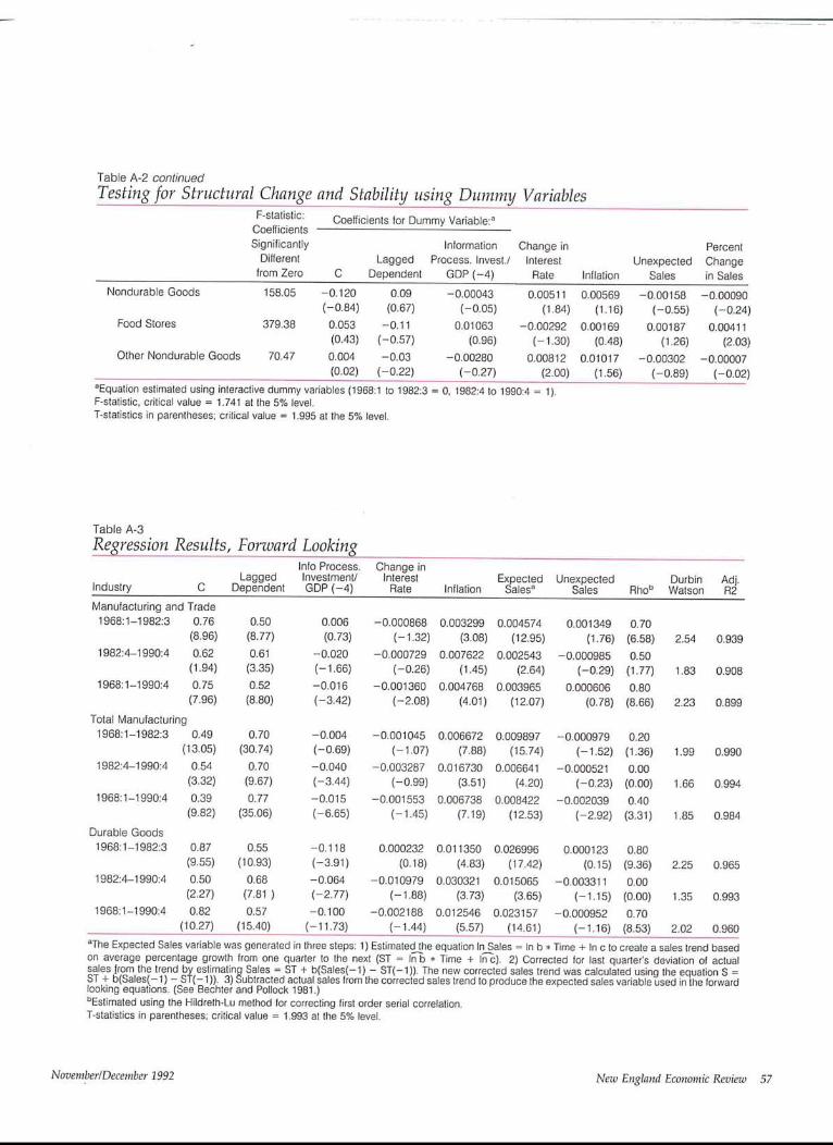
Table A-2 continuedTesting for Structural Change and Stability using Dum~ny Variables

F-statistic: Coefficients for Dummy Variable:"CoefficientsSignificantly Information Change in

Different Lagged Process. Invest./ Interestfrom Zero C Dependent GDP (-4) Rate

Nondurable Goods 158.05 -0.120 0.09 -0.00043 0.00511(-0.84) (0.67) (-0.05) (1.84)

Food Stores 379.38 0.053 -0.11 0.01063 -0.00292(0.43) (-0.57) (0.96) (- 1.30)

Other Nondurable Goods 70.47 0.004 -0.03 -0.00280 0.00812(0.02) (-0.22) (-0.27) (2.00)

aEquation estimated using interactive dummy variables (1968:1 to 1982:3 = O, 1982:4 to 1990:4 = 1).F-statistic, critical value = 1.741 at the 5% level.T-statistics in parentheses; critical value = 1.995 at lhe 5% level.

PercentUnexpected Change

Inflation Sales in Sales

0.00569 -0.00158 -0.00090(1.16) (-0.55) (-0.24)

0.00169 0.00187 0.00411(0.48) (1.26) (2.03)

0.01017 -0.00302 -0.00007(1.56) (-0.89) (-0.02)

Table A-3Regression Results, Forward Looking

Into Process. Change inLagged Investment/ Interest Expected Unexpected Durbin Adj.

industry C Dependent GDP (-4) Rate Inflation Salesa Sales Rhob Watson R2Manufacturing and Trade1968:1-1982:3 0.76 0.50 0.006 -0.000868 0.003299 0.004574 0.001349 0.70

(8.96) (8.77) (0.73) (-1.32) (3.08) (12.95) (1.76) (6.58) 2.54 0.9391982:4-1990:4 0.62 0.61 -0.020 -0.000729 0.007622 0.002543 -0.000985 0.50

(1.94) (3.35) (-1.66) (-0.26) (1.45) (2.64) (-0.29) (1,77) 1.83 0.9081968:1-1990:4 0.75 0.52 -0.016 -0.001360 0.004768 0.003965 0.000606 0.80

(7.96) (8.80) (-3.42) (-2.08) (4.01) (12.07) (0.78) (8.66) 2.23 0.899Total Manufacturing

1968:1-1982:3 0.49 0.70 -0.004 -0.001045 0.006672 0.009897 -0.000979 0.20(13.05) (30.74) (-0.69) (-1.07) (7.88) (15.74) (-1.52) (1.36) 1.99 0.990

1982:4-1990:4 0.54 0.70 -0.040 -0.003287 0.016730 0.006641 -0.000521 0.00(3.32) (9.67) (-3.44) (-0.99) (3.51) (4.20) (-0.23) (0.00) 1.66 0.994

I968:1-1990:4 0.39 0.77 -0.015 -0.001553 0.006738 0.008422 -0.002039 0.40(9.82) (35.06) (-6.65) (-1.45) (7.19) (12.53) (-2.92) (3.31) 1.85 0.984

Durable Goods1968:1-1982:3 0.87 0.55 -0.118 0.000232 0.011350 0.026996 0.000123 0.80

(9.55) (10.93) (-3.91) (0.18) (4.83) (17.42) (0.15) (9.36) 2.25 0.9651982:4--1990:4 0.50 0.68 -0.064 -0.010979 0.030321 0.015065 -0.003311 0.00

(2.27) (7.81) (-2.77) (-1.88) (3.73) (3.65) (-1.15) (0.00) 1.35 0.9931968:1-1990:4 0.82 0.57 -0.100 -0.002188 0.012546 0.023157 -0.000952 0.70

(10.27) (15.40) (-11.73) (-1.44) (5.57) (14.61) (-1.16) (8.53) 2.02 0.960aThe Expected Sales variable was generated in three steps: 1) Estimated the equation In Sales = In b ,~ Time + In c to create a sales trend basedon average percentage growth from one quarter to the next (ST = In"~ * Time + I~-"&). 2) Corrected for last quarter’s deviation of actualsales Item the trend by estimating Sales = ST + b(Sales(-1) - ST(-1)). The new corrected sales trend was ca cu ated using the equation S =ST + b(Sales(- 1) - ST(- 1)). 3) Sublracted actual sales from the corrected sales trend o produce the expected sa es var abe used in the forwardlooking equations. (See Bechter and Pollock 1981.)bEstimated using the Hildreth-Lu method for correcling first order serial correlation.T-statislics in parentheses; critical value = 1.993 at the 5% level.

November/December 1992 New England Econoznic Review 57

Table A-3 continued (2)

Regression Results, Forward Looking

Industry CNondurable Goods1968:1-1982:3 0.24 0.81

(4.31) (19.33)1982:4-1990:4 0.40 0.69

(2.60) (6.69)1968:1-1990:4 0.28 0.78

(6.27) (23.04)Manufacturing Durable GoodsPrimary Metals1968:1-1982:3 0.18 0.86

(2.06) (17.84)1982:4-1990:4 -0.13 0.86

(-1.19) (27.25)1968:1-1990:4 0.22 0.84

(2.74) (26.16)

Info Process. Change inLagged Investment/ Interest Expected Unexpected

Dependent GDP (-4) Rate Inflation Salesa Sales

-0.020 -0.001463 0.004412 0.009304 -0.005544(-3.87) (-1.38) (5.34) (6.18) (-5.35)-0,024 -0.000025 0.009359 0,008884 0.001049(-2.67) (-0.01) (2.18) (2.75) (0.48)-0.012 -0.001669 0.003510 0.009458 -0.003725(-6.13) (-1.56) (6.19) (7.02) (-3.94)

0.047(0.87)

O.O07(0.51)

0.004(0.39)

Fabricated Metals1968:1-1982:3 0.57 0.68 0.003

(3.54) (7.40) (0.06)1982:4-1990:4 0.89 0.63 -0.036

(3.19) (6.36) (-2.19)1968:1-1990:4 0.49 0.73 -0.008

(5.09) (15.05) (-1.14)Industrial & Commercial Machinery1968:1-1982:3 0.88 0.67 -0.039

(4.90) (9.82) (- 1.12)1982:4-1990:4 0.19 0.88 -0.036

(0.65) (13.48) (-0.82)1968:1-1990:4 0.44 0.83 -0.066

(4.33) (25.65) (-4.74)Electronic Machinery

1968:1-1982:3 1.20 0.44 0.028(5.99) (4.67) (0.88)

1982:4-1990:4 0.70 0.76 -0.078(1.54) (5.18) (-2.25)

1968:1-1990:4 1.17 0.50 - 0.045(5.17) (5.66) (-1.72)

Motor Vehicles & Parts1968:1-1982:3 0.46 0.59 -0.094

(5.99) (7.77) (-3.97)1982:4-1990:4 0.30 0.62 -0.016

(2.32) (5.21) (-1.62)1968:1-1990:4 0.40 0.62 -0.041

(5.78) (9.03) (-4.93)Other Transportation1968:1-I982:3 0.30 0.91 0.021

(1.37) (16.31) (0.47)0.42 0.86 -0.020

(1.10) (10.44) (-0.72)0.24 0.93 0.010

(1.63) (26.37) (0.98)

1982:4-1990:4

1968:1-1990:4

Durbin Adj,Rhob Watson R2

2.16 0.941

1.97 0.978

1.88 0.98O

-0.004547 0.014066 0.185820 -0.001270 0.50(-1.11) (2.44) (14,16) (-1.23) (3.87) 2.28 0,961

0.011022 0.091662 0.161200 -0.005019 -0.20(1.11) (8.16) (5.93) (-2.78) (-1.02) 1.79 0.994

-0.003498 0.021613 0.185620 -0.001348 0.60(-0.95) (4.96) (15.62) (-1.56) (6.22) 2.33 0.942

0.001967 0.015362 0.186570 -0.000147 0.60(0.52) (2.67) (6.94) (-0.08) (4.27) 2.04 0.872

-0.002723 -0.008899 0.172270 0.001027 -0.10(-0.47) (-0.89) (6.18) (0.47) (-0.44) 1.90 0.984

-0.000235 0.013336 0.171450 -0.000606 0.50(-0.08) (3.83) (9.11) (-0.50) (4.57) 2.11 0.910

-0.000919 0.013528 0.181830 -0.000926 0.70(-0.44) (3.58) (9.19) (-0.48) (6.58) 2.37 0.930

-0.007479 0.026713 0.060422 -0.004146 0.60(-0.98) (1.44) (4.15) (-1.80) (3.07) 1.72 0.982

-0.004192 0.016832 0.083457 -0.006386 0.60(-1.58) (4.64) (6.48) (-4.28) (6.08) 2.06 0.979

0.001455 0.013738 0.229380 0.002766 0.70(0.65) (3.18) (9.88) (1.68) (5.58) 1.92 0.871

-0.006367 0.024408 0.141570 -0.000824 0.70(-0.99) (1.51) (4.55) (-0.30) (5.22) 2.04 0.843

-0.001052 0.011638 0.188050 0.001572 0.90(-0.54) (2.67) (10.95) (1.13) (13.22) 2.05 0.795

0.000136 0.008213 0.080706 -0.000856(0.03) (2.00) (8.58) (- 1.29)

-0.008860 0.006711 0.045395 -0.000313(-1.31) (0.65) (6.19) (-0.42)

-0.002812 0.004725 0.064700 -0.001066(-0.68) (1.68) (8.79) (-1.86)

1.93 0.864

2.01 0.880

2.03 0,929

0.005855 0.002447 0.334680 -0.008161(0.68) (0.34) (4.64) (-2.33)

-0.011475 0.059067 0.553240 0.004287(-0.56) (1.82) (6.01) (0.81)

0.006079 0.003576 0.388850 -0.005982(0.78) (0.80) (7.38) (-2.20)

1.69 0.911

1.42 0.917

1.57 0.945


Table A-3 continued (3)Regression Results, Forward Looking

Info Process.Lagged InvestmenlJ

Industry C Dependent GDP (-4)

Change inInterest Expected Unexpected Durbin Adj.

Rate Inflation Sales" Sales Rho~ Watson R2

Other Durable Goods1968:1-1982:3 0.55 0.69 0.023

(4.38) (9.37) (1.00)1982:4-1990:4 0.74 0.67 -0.044

(2.98) (6.85) (-2.61)1968:1-1990:4 0.46 0.75 -0.015

(4.91) (15.41) (-2.66)

Manufacturing Nondurable GoodsFood and Kindred Products1968:1-1982:3 0.21 0,81

(2.03) (8.31)1982:4-1990:4 0.24 0.74

(2.21) (8.I2)1968:1-1990:4 0.23 0.79

(3.26) (12.26)Paper & Allied Products1968:1-1982:3 0.74 0.35

(6.43) (4.22)1982:4-1990:4 0.71 0.43

(4.65) (3.81)1968:1-1990:4 0.72 0.39

(6.97) (4.87)

Chemicals and Allied Products1968:1-1982:3 0.42 0.77

(5.35) (18.440.64 0.61(2.81) (5.330.45 0.74

(5.57) (17.12

Products0.10 0.84(2.22) (13.400.58 0.40(3.20) (2.600.08 O.87(2.17) (19.00

Products0.29 0.80(4.38) (15.740.18 0.82

(1.57) (12.29)0.33 0.76

(7.25) (23.40)

1982:4-1990:4

1968:1-1990:4

Petroleum and Coal1968:1-1982:3

1982:4-1990:4

1968:1-1990:4

Rubber and Plastic1968:1-1982:3

1982:4-1990:4

1968:1-1990:4

-0.000478 0.006258 0.107910 -0.001116 0.60(-0.25) (2.20) (7.79) (-0.82) (4.66) 1.80 0.929

0.000363 0.002387 0.090436 0.000917 0.30(0.07) (0.25) (4.87) (0.43) (1.23) 1.79 0.968

-0,001075 0.007661 0.093841 -0.001692 0.60(-0.60) (3.36) (8.69) (- 1.59) (5.56) 2.02 0.922

-0.005 0.000193 -0.000364 0.034511 -0.000065(-0.51) (0.10) (-0.23) (3.03) (-0.05) 1.91 0.563-0.010 0.000535 0.003917 0.050413 0.001126(- 1.34) (0.22) (0.98) (4.46) (0.47) 2.44 0.974-0.015 0.000403 0.001068 0.030770 -0.000282(-3.36) (0.27) (1.22) (4.09) (-0.25) 1.94 0,953

0.048 -0.002573 0.007255 0.253640 0.001562 0.90(1.20) (-2.10) (2.44) (8.37) (1.34) (12.05) 2.25 0.840

-0.002 -0.002345 0.010222 0.187890 0.001571 -0.10(-0.43) (-0.57) (1.97) (4.63) (0.71) (-0.45) 2.01 0.868

0.011 -0.002366 0.009298 0.221810 0.001094 0.80(1.41) (-1.90) (3.80) (8.49) (1.02) (10.19) 2.36 0.785

-0.047 0.001872 0.005559 0.131320 -0.001785 0.30(-3.51) (0.87) (2.58) (10.60) (-1.45) (2.14) 2.05 0.949-0.022 0.004647 0.007039 0.115170 0.003048 0.00(-2.37) (0.73) (0.79) (5.51) (1.07) (0.00) 1.91 0.945-0.019 0.001347 0.003151 0.124050 -0,000913 0.30(-4.37) (0.62) (2.17) (11.28) (-0.78) (2.65) 1.91 0.945

0.002 0.000497 0.004341 0.041708 -0.002785(0.18) (0.24) (2.80) (5.38) (-2.53) 1.70 0.901

-0.061 -0.010617 0.025814 0.007299 0.001310(-3.42) (- 1.38) (2.08) (0.37) (0.52) 1.87 0.879

0.000076 -0.001782 0.003589 0.032868 -0.000943(0.03) (-0.69) (2.70) (3.63) (-0.78) 1.78 0.846

-0.022 0.001622 0.007296 0.246260 -0.002728(-1.37) (0.55) (2.29) (6.06) (-2.63) 1.48 0.958

-0.005 0.007969 0.016635 0.169780 -0.002325(-0.57) (1.64) (2.31) (5.35) (-1.71) 2.20 0.968-0.018 0.001276 0.010258 0.205730 -0.002625(-5.24) (0.53) (4.96) (8.35) (-3.44) 1.59 0.979

aThe Expected Sales variable was generated in three steps: 1) Estimate.._..d the equatio~n In Sales = In b .~ Time + In c ~o create a sales trend basedon average percentage growth from one quarter to the next (ST = In b ,, Time + In c). 2) Corrected for last quarter’s deviation of actual salesfrom t.he trend by estimating Sales = ST + b(Sales(-1) - ST(-1)). The new corrected sales trend was calculated using the equation S =ST + b(Sales(- 1 ) - ST(- 1 )). 3) Subtracted actual sales from the corrected sales trend to produce the expected sales variable used in the forwardlooking equations. (See Bechter and Pollock 1981.)bEstirnated using the Hildreth-Lu melhod for correcting first order serial correlation.T-statistics in parentheses; critical value = 1.993 at the 5% level.

NovembeHDecember 1992 New England Economic Review 59


Info Process. Change inLagged Investment/ Interest

Industry C Dependent GDP (-4) RaleExpected Unexpected Durbin Adj.

Inflation Salesa Sales Rho~ Watson R2

Other Nondurable Goods1968:1-1982:3 1.35 0.29

(6.53) (2.63)1982:4-1990:4 0.81 0.57

(2.90) (4.08)1968:1-1990:4 1.07 0.43

(6.91) (5.25)Wholesale

1968:1-1982:3 0.29 0.76(2.47) (8.43)

1982:4-1990:4 0.85 0.36(2.49) (1.47)

1968:1-1990:4 0.35 0.72(3.52) (9.74)

Wholesale Durable Goods1968:1-1982:3 0.60 0.66

(4.33) (9.01)1982:4-1990:4 0.83 0.59

(4.04) (6.94)1968:1-1990:4 0.38 0.78

(5.37) (21.69)Wholesale Nondurable Goods

1968:1-1982:3 0.12 0.87(1.73) (12.24)

1982:4-1990:4 0.16 0.81(1.22) (5.43)

1968:1-1990:4 0.12 0.86(2.69) (17.40)

Retail1968:1-1982:3 0.23 0.85

(2.24) (11.52)1982:4-1990:4 1.01 0.26

(3.22) (1.24)1968:1-1990:4 1.02 0.26

(5.81) (2.07)Retail Durable Goods

1968:1-1982:3 0.56 0.74(3.86) (9.45)

1982:4-1990:4 1.08 0.49(4.77) (4.18)

1968:1-1990:4 0.62 0,70(5.22) (11.14)

-0.105 -0.003700 0.008338 0.094582 0.001949 0.60(-5.22) (-2.54) (3.21) (6.73) (1.15) (4,26) 1.93 0.824-0.052 0.004419 0.002408 0.072638 -0,000347 0.30(-2.70) (0,84) (0.26) (3.76) (-0.14) (1.21) 1.94 0.952

-0.072 -0.003030 0.005475 0.083116 0.000283 0.40(-6.93) (-2.01) (3.60) (7.94) (0.20) (3.24) 1.80 0.971

0.010 -0.000623 0.001331 0.010493 -0.002279 0.20(1.02) (-0.42) (0.96) (5.64) (- 1.95) (1.09) 2.03 0.844

-0.009 -0.000846 0.003274 0.012161 0.005049 0.60(-0.96) (-0.25) (0.40) (4.08) (1.90) (2.05) 2.00 0.601-0.002 -0.001078 0.002525 0.009900 -0.001839 0.30(-0.74) (-0.82) (2.82) (6.68) (-1,86) (2.11) 2.12 0.799

0.053 0.000038 0.001966 0.046709 -0.001174 0.60(2.36) (0.02) (0.69) (8.01) (-0.86) (4.26) 2.29 0.930

-0.023 -0.008176 0.003949 0.032260 -0.000194 0.00(-2.08) (-1.16) (0.41) (5.01) (-0.06) (0.00) 2.14 0.959

-0.002 -0.001923 0.008422 0.033585 -0.003374 0.30(-0.64) (-0.93) (6.09) (9.47) (-2.96) (2.50) 1.95 0.940

-0.005 0.000303 -0.000467 0.010327 -0.001386(-0.45) (0.!7) (-0.35) (2.96) (-1.28)

0.000216 -0.003218 -0.000576 0.008894 -0.000395(0,04) (-1.04) (-0.09) (2.91) (-0.26)

-0.001 -0.000287 -0.001008 0.009783 -0.001219(-0.71) (-0.20) (-1.22) (4.30) (-1.49)

2.01 0.845

1.65 0.738

1.94 0.837

0.009 -0.000708 -0.003696 0.012368 -0.002456 -0.10(1.18) (-0.43) (-2.70) (4.79) (-t.48) (-0.64) 1.94 0.853

0.008 0.001560 0.016083 0.021617 0.007404 0.80(0.26) (0.28) (1.58) (5.12) (2.46) (4.97) 2.00 0.582

0.024 -0.001080 -0.001102 0.018405 0.003886 0.70(3.47) (-0.79) (-0.50) (7.72) (2.63) (6.61) 2.19 0.618

-0.005 -0.002792 -0.001852 0.059260 -0.001687(-0.24) (-0.58) (-0.43) (5.80) (-1.01)

0.009 0.014260 -0.024136 0.061781 0.006347(0.72) (1.28) (-1.49) (6.40) (2.14)

-0.009 -0.000688 -0.000285 0.058438 -0.000830(-2.01) (-0.17) (-0.09) (8.50) (-0.59)

Auto Dealers1968:1-1982:3 0.66 0.59 0.002

(4.61) (5.93) (0.05)1982:4-1990:4 0.77 0.55 0.056

(3.97) (3.97) (1.83)1968:1-1990:4 0.54 0.68 0.010

(5.55) (9.84) (1.18)

2.12 0.842

1.33 0.727

1.86 0.843

0.000363 0.005451 0.077732 -0.001164(0.05) (0.79) (4.21) (-0.73)

0.025766 -0.040068 0.107390 0.004648(1.48) (-1.54) (6.03) (1.55)

0.007836 -0.000651 0.097011 -0.000005(1.29) (-0.15) (7.95) (-0.004)

2.05 0.769

1.51 0.851

1.89 0.793

60 November/December 1992 Nezo England Economic Review


Info Process. Change i~-Lagged Investment/ Interest Expected Unexpected Durbin Adj.

Industry C Dependent GDP (-4) Rate Inflation Sales" Sales Rhob Watson R2

Retail Other Durable Goods1968:1-1982:3 0.37 0.88 -0.031 -0.005842-0.004211 0.181570 -0.004458

(2.63) (16.67) (-1.88) (-1.64) (-1.55) (7.58) (-2.20) 1.69 0.8921982:4-1990:4 0.90 0.65 -0.049 -0.007404 0.012487 0.062977 -0.004029

(3.10) (6.79) (-2.72) (-0.99) (1.06) (2.38) (-0.92) 2.03 0.9561968:1-1990:4 0.50 0.82 -0.027 -0.009542 -0.001698 0.123800 -0.005883

(4.10) (18.35) (-4.00) (-2,99) (-0.89) (6.91) (-3.20) 1.65 0.964

Retail Nondurable Goods1968:1-1982:3 0.35 0.70 0.001 -0.001785 -0.002872 0.018214 0.001259 0.30

(2.66) (6.19) (0.17) (-1.84) (-2.71) (3.91) (0.65) (1.53) 2.02 0.7411982:4-1990:4 0.68 0.36 0.021 -0.001642 0.007846 0.018534 0.002433 0.60

(2.30) (1.35) (1.87) (-0.59) (1.26) (2.34) (0.64) (3.03) 2.64 0.7021968:1-1990:4 0.29 0.75 0.008 -0.001540 -0.003317 0.018029 0.000877 0.30

(3.53) (10.25) (3.14) (-1.75) (-3.85) (4.97) (0.55) (2.19) 2.13 0.918Food Stores

1968:1-1982:3 0.19 0.69 0.020 -0.000427 -0.000433 0.037242 -0.000188(4.11) (9.19) (3.68) (-0.55) (-0.71) (5.55) (-0.19) 1.69 0.903

1982:4-1990:4 0.25 0.59 0.023 -0.003380 0.000326 0.011745 0.000625(1.95) (2.91) (2.17) (-1.44) (0.08) (0.89) (0.33) 2.36 0.945

1968:1-1990:4 0.20 0.67 0.020 -0.000852 -0.000437 0.029571 0.000059(4.64) (9.32) (5.02) (-1.10) (-1.06) (5.02) (0.07) 1.97 0.980

Retail Other Nondurable Goods1968:1-1982:3 0.38 0.74 -0.008 -0.002663 -0.003932 0.027798 0.001699 0.30

(2.47) (7.04) (-0.66) (-1.88) (-2.53) (3.31) (0.72) (1.58) 2.11 0.8211982:4-1990:4 0.91 0.30 0.007 -0.001651 0.013722 .030712 0.002663 .70

(2.89) (1.35) (0.61) (-0.51) (1.98) (2.91) (0.72) (4.55) 2.37 0,5331968:1-1990:4 0.31 0.79 0.002 -0,002051 -0.004294 0.027434 0.000673 0.30

(3.25) (11.82) (1.07) (-1.65) (-3.48) (4.33) (0.35) (2.25) 2.07 0.838aThe Expected Sales variable was generated in three steps: 1) Estimat....~ed the equati£~n In Sales = In b ,~ Time + In c to create a sales trend basedon average percentage growth from one quarter to the next (ST = In b * Time + In c). 2) Corrected for last quarter’s deviation of actual salesfrom t.he trend by estimating Sales = ST + b(Sales(-1) - ST(-1)). The new corrected sales trend was calculated using the equation S =ST + b(Sales(-1) - ST(- 1)). 3) Subtracted actual sales from the corrected sales trend to produce the expected sales variable used in the forwardlooking equations. (See Bechter and Pollock 1981.)bEstimated using the Hildreth-Lu method for correcting first order serial correlation.T-statistics in parentheses; critical value = 1.993 at the 5% level.

Nove~nbeHDecember 1992 New England Economic Review 61

Table A-4Kinked Time Regression Results1968:1 to 1982:3, 1982:4 to 1990:4

IndustryManufacturing & Trade

Manufacturing

Durable Goods

Nondurable Goods

Manufacturing Durable Goods:Primary Metals

Fabricated Metals

Machinery, Except Electrical

Electrical Machinery

Motor Vehicles & Parts

Other TransportationEquipment

Other Durable Goods

Manufacturing Nondurable GoodsFood & Kindred Products

Paper & Allied Products

Chemicals & Allied Products

Petroleum & Coal Products

Rubber & Plastic Products


Merchant Wholesalers

Wholesale Durable Goods

Wholesale Nondurable Goods

Retail Trade

Retail Durable Goods

Automotive Dealers

Other Durable Goods

Retail Nondurabte Goods

Food Stores


LaggedC Dependent Time

0.48 0.70 0.000083(7.53) (16.96) (0.56)0.41 0.76 0.000034

(8.99) (28.16) (0.18)0.51 0.75 0.000837

(10.48) (32.24) (2.85)0.23 0.82 -0.000545

(4.12) (19.17) (-4.03)

Interaclive Dummy Dummy Change in(Time * Dummy (82:4 to Interest

Variable) 90:4 = 1) Rate Inflation

-0.001962 0.12 -0.002675 0.001495(-4.59) (4.56) (-3.05) (1.42)

-0.003517 0.24 -0.003368 0.004943(-6.04) (6.28) (-3.16) (3.85)

-0.006829 0.44 -0.005443 0.005432(-7.60) (7.65) (-3.50) (3.00)

-0.000789 0.07 -0.002329 0.004301(-2.06) (2.70) (-2.11) (4.16)

0.15 0.92(2.65) (35.81)0.52 0.72

(4.55) (11.16)1.11 0.58

(7.46) (11.39)1.14 0.49

(7.03) (6.70)0.32 0.71

(5.06) (10.61)

0.75(2.95)0.49

(4.70)

0.79(12.53)

0.74(12.63)

0.000010 0.001265 - O. 12(0.01) (0.73) (- 1.09)

0.001976 -0.005909 0.33(2.41) (-2.86) (2.55)

0.000845 -0.023816 1.45(0.78) (-6.24) (6.25)

0.002051 -0.011156 0.69(2.61) (-5.08) (5.06)

-0.001366 -0.001338 0.10(-2.50) (- 1.51) (1.65)

0.001939 -0.005840 0.50(1.42) (-2.04) (2.46)

0.000582 -0.003968 0.24(1.22) (-2.89) (2.75)

0.23 0.79 -0.000140 -0.001071 0.05(2.70) (9.83) (-0.65) (- 1.70) (1.33)0.26 0.79 0.000279 -0.000293 0.01

(6.40) (23.83) (1.24) (-0.70) (0.52)0.33 0.84 -0.001354 0.000278 0.02

(4.12) (19.51) (-3.66) (0.40) (0.33)O. 17 0.75 -0.000072 - 0.002203 O. 18

(3.51) (11.70) (-0.22) (-2.57) (2.98)0.25 0.83 -0.000122 -0.000933 0.03

(4.73) (20.77) (-0.37) (-1.17) (0.70)1.26 0.32 -0.002429 -0.005034 0.31

(7.19) (3.59) (-2.80) (-2.93) (2.95)0.98 0.29 0.000390 - 0.001997 0.11

(6.99) (2.81) (0.65) (- 1.48) (1.32)0.32 0.85 0.000660 -0.001334 0.04

(4.87) (26.34) (2.24) (- 1.84) (0.93)0.90 0.04 -0.001900 0.003341 -0.19

(7.45) (0.29) (-2.71) (2.23) (-2.02)0.56 0.63 0.000502 0.000436 -0.04

(5.71) (8.97) (2.41) (0.87) (-1.16)0.84 0.61 0.000763 -0.001311 0.01

(6.10) (8.57) (!.34) (-1.08) (0.15)0.82 0.50 0.001115 0.003972 -0.35

(6.34) (5.70) (1.25) (1.89) (-2.41)0.59 0.81 -0.000023 -0.004039 0.23

(4.84) (18.12) (-0.07) (-3.87) (3.58)0.33 0.73 - 0.000116 0.000717 -0.03

(5.15) (13.33) (-0.92) (2.14) (-1.59)0.23 0.79 -0.000140 -0.001071 0.05

(2.70) (9.83) (-0.65) (- 1.70) (1.33)0.53 0.65 -0.000634 0.001303 -0.06

(2.62) (4.61) (-1.53) (1.41) (-1.21)

-0.008593 0.006087(-1.80) (1.57)

-0.001066 0.002447(-0.36) (0.54)

-0.002525 0.012374(- 1.46) (3.48)

-0.004013 0.004645(-2.19) (1.29)

-0.006174 0.002902(-1.82) (0.74)

0.000776 -0.002133(0.11) (-0.26)

-0.003445 0.003795(-1.82) (1.38)

-0.000033 -0.000063(-0.02) (-0.05)

-0.003014 0.002339(-1.89) (1.54)

-0.000009 0.001796(-0.00) (0.73)

-0.002808 0.004870(-1.10) (2.37)

0.000667 0.004089(0.28) (1.62)

-0.003936 0.007265(-2.99) (2.56)

-0.001114 -0.004096(- 1.05) (- 1.81 )

-0.003229 -0.003378(-1.47) (-1.67)

-0.000446 -0.002704(-0.40) (-1.17)

-0.000859 -0.004717(-0.55) (-3.24)

-0.004474 -0.004345(-0.99) (-1.01)

-0.000351 0.002022(-0.05) (0.31)

-0.007460 -0.009074(-2.57) (-3.43)

-0.001588 -0.002899(- 1.83) (-3.94)

-0.000033 -0.000063(-0.02) (-0.05)

-0.002470 -0.003723(-2.02) (-2.39)

62 November/December 1992 Nezo England Economic Review

Table A-4 continuedKinked Time Regression Results1968:1 to 1982:3, 1982:4 to 1990:4

PercentUnexpected Change in Durbin Adjusted

Sales Salesa Rho":’ Watson R2-0.005125 -0.014 0.30

(-8.38) (-8.91) (2.54) 2.07 0.966-0.006596 -0.017 0.30

(- 12.59) (- 11.70) (2.62) 2.02 0.988-0.007833 -0.024 0.30

(-14.96) (-14.97) (2.70) 1.95 0.990-0.006803 -0.007

(-7.88) (-4.45) 1.96 0.978

-0.009847 -0.025(-12.17) (-13.79) 1.64 0.981

-0.006166 -0.027 0.50(-6.78) (-9.53) (4.31) 2.09 0.919

-0.006862 -0.032 0.80(-7.49) (-12.65) (13.04) 2.23 0.970

-0.004298 -0.027 0.70(-4.45) (- 11.48) (7.32) 1.95 0.888

-0.003277 -0.011(-8.34) (-11.45) 2.08 0.949

-0.013558 -0.048 0.30(-7.40) (-7.81) (2.44) 2.15 0.906

-0.006581 -0.019 0.50(-8.37) (-7.86) (4.23) 1.89 0.937

-0.002234 -0.007(-2.17) (-2.86) 1.97 0.949

-0.006026 -0.016(-6.76) (-9.57) 1.84 0.955

-0.007885 -0.021 0.30(-8.80) (-10.23) (2.58) 1.94 0.946

-0.002892 -0.007(-3.21) (-3.29) 1.75 0.853

-0.006030 -0.013(-9.47) (-8.48 2.05 0.980

-0.002032 -0.019 0.80(-1.91) (-7.74) (10.01) 1.87 0.852

-0.001266 -0.019 0.80(-1.57) (-9.06) (9.83) 2.10 0.636

-0.008432 -0.019(-7.60) (-10.32) 1.74 0.965

0.000274 -0.011 0.80(0.47) (-6.34) (10.75) 1.84 0.388

-0.004306 -0.018(-3.75) (-6.69) 1.94 0.898

-0.005736 -0.022(-4.79) (-6.84) 2.15 0.822

-0.004199 -0.018(-3.59) (-5.21) 2.08 0.748

-0.010560 -0.027(-7.71) (-9.06) 1.78 0.971

-0.002719 -0.015(-2.19) (-6.56) 1.55 0.958

-0.002234 -0.007(-2.17) (-2.86) 1.97 0.949

-0.002633 -0.016 0.40(-1.77) (-4.09) (2.11) 2.10 0.799

aPolynomial Distributed Lag (first degree polynomial, 3 quartersincluding current quarter, far endpoinl constraint).bEstimated using the Hildreth-Lu method for correcting first orderserial correlation.Coefficients shown are the sum of the estimated lagged coefficienls.T-statistics in parentheses; critical value = 1.993 at the 5% level.

Figure A-1

Inventory-to-Sales Ratios

Durable Goods Manufacturing." Selected Industries

Ratios based on 1982 Dollars

2.2

2.0

1.8

1.6

1.4

1.2

1.0

.8

.6

3.0

2.5

01967 1969 1971 1973 1975 1977 1979 1981 1983 1985 1987 1989 1991

1.5

Nondurable Goods Manufacturing

Chemical andAllied Products

/

Rubcer and

.4 i i , , i , i , , i , .1967 1969 1971 1973 1975 1977 1979 1981 1983 1985 1987 1989 1991

1.0

Retail Trade

Automotive Dealers ¯

1967 1969 1971 1973 1975 1977 1979 1981 1983 1985 1987 1989 1991

Quarterly data, seasonally adjusted.Shaded areas represent recessions.Source: U.S. Bureau of Economic Analysis.

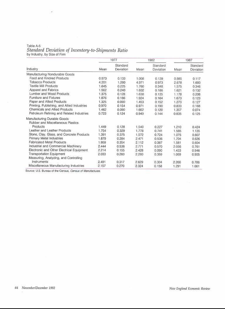
Table A-5Standard Deviation of Inventory-to-Shipments Ratioby Industry, by Size of Firm

1977 1~82 1987

Industry MeanManufacturing Nondurable Goods

Food and Kindred Products 0.973 0.133Tobacco Products 4.201 1.260Textile Mill Products 1.645 0.225Apparel and Fabrics 1.562 0.240Lumber and Wood Products 1.375 0.128Furniture and Fixtures 1.876 0.186Paper and Allied Products 1.325 0.090Printing, Publishing, and Allied Industries 0.970 0.154Chemicals and Allied Products 1.462 0.090Petroleum Refining and Related Industries 0.723 0.124

Manufacturing Durable GoodsRubber and Miscellaneous Plastics

Products 1.449 0.128Leather and Leather Products 1.754 0.329Stone, Clay, Glass, and Concrete Products 1.391 0.375Primary Metal Industries 1.879 0.284Fabricated Metal Products 1.959 0.354Industrial and Commercial Machinery 2.444 0.536Electronic and Other Electrical Equipment 2.214 0.155Transportation Equipment 2.033 0.260Measuring, Analyzing, and Controlling

Instruments 2.491 0.317Miscellaneous Manufacturing Industries 2.157 0.270

MeanStandardDeviation

StandardDeviation

StandardMean Deviation

1.008 0.139 0.885 0.1174.971 0.973 2.678 1.6931.760 0.348 1.575 0.3461.602 0.186 1.621 0.1321.630 0.135 1.178 0.2081.924 0.164 1.673 0.1231.453 0.152 1.273 0.1270.971 0.190 0.833 0.1681.662 0.120 1.357 0.0740.949 0.144 0.835 0.125

1.540 0.227 1.210 0.4241.778 0.741 1.585 1.1351.572 0.724 1.075 0.6072.471 0.536 1.704 0.6262.112 0.387 1.581 0.6042.771 0.570 2.066 0.7612.428 0.090 1.433 0.9462.280 0.359 1.069 0.905

2.629 0.304 2.266 0.7862.324 0.158 1.291 1.061

Source: U.S. Bureau of the Census, Census of Manufactures.


Aepel, Timothy. 1992. "Ford Reaches Fork in Road in Its EuropeanOperations: With Japanese Threat Looming, ’Lean Production’Looks Like the Future." The Wall Street Journal, October 6.

Akhtar, M.A. 1983. "Effects of Interest Rates and Inflation onAggregate Inventory Investment in the United States." TheAmerican Economic Review, vol. 73, no. 3 (June), pp. 319-28.

Arthur Andersen and Andersen Consulting. 1992. "World Retail-ing Highlights." International Trends in Retailing, vol. 9, no. 1,Summer, pp. 49-96.

Bechter, Dan M. and Stephen H. Pollock. 1981. "Inventory Sensi-tivity to Interest Rates in Selected Manufacturing and TradeSectors." Federal Reserve Bank of Kansas City, Research Work-ing Paper 81-10, September.

Bechter, Dan M. and Stephen Stanley. 1992. "Evidence of Im-proved Inventory Contro!." Federal Reserve Bank of Richmond,Economic Review, January/February, pp. 3-12.

Berger, Susan. 1992. "Moving Macaroni." The Federal ReserveBank of Boston Regional Review, Vol. 2, No. 1 (Winter), p. 3.

Betancourt, Roger and Harry Kelejian. 1981. "Lagged EndogenousVariables and the Cochrane-Orcutt Procedure." Econometrica,vol. 49, no. 4 (July), pp. 1073-78.

Blinder, Alan S. 1981. "Inventories and the Structure of MacroModels." AEA Papers and Proceedings, vol. 71, no. 2 (May), pp.11-16.

¯ 1986. "More on the Speed of Adjustment in InventoryModels." Journal of Money, Credit and Banking, vol. 18, no. 3(August), pp. 355-65.

Blinder, Alan S. and Louis J. Maccini. 1991. "Taking Stock: ACritical Assessment of Recent Research on Inventories." Journalof Economic Perspectives, vol. 5, no. 1 (Winter), pp. 73-96.

Bryant, Adam. 1992. "Colt’s New Cltief Likes to Fix Businesses."The New York Times, May 15, p. DS.

Burt, David N. 1989. "Managing Suppliers Up to Speed." HarvardBusiness Review, July-August, pp. 127-35.

Caballero, Ricardo J. and Eduardo M.R.A. Engel. 1991. "Dynamic(S,s) Economies." Econometrica, vol. 59, no. 6 (November), pp.1659-86.

Chain Store Executive. 1991, Section three, March.Cuthbertson, Keith and David Gasparro. 1992. "The Determinants

of Manufacturing Inventories in the UK." (Bank of England,Economics Division. Unpublished. February.

Forrester, Jay W. 1961. Industrial Dynamics. Cambridge, MA.: TheM.I.T. Press, pp. 21-42.

Hay, Donald and Helen Louri. 1991. "Investment in Inventories:An Empirical Microeconomic Model of Firm Behaviour." Insti-tute of Economics and Statistics, Applied Economics DiscussionPaper No. 123. University of Oxford, Oxford, England. October.

Henderson, Yolanda K. with Jeffrey B. Liebman. 1992. "CapitalCosts, Industrial Mix, and the Composition of Business Invest-ment." Federal Reserve Bank of Boston, Nezo England EconomicReview, January/February, pp. 67-92.

Irvine, F. Owen, Jr. 1981. "Merchant Wholesaler Inventory Invest-

ment and the Cost of Capita!." AEA Papers and Proceedings, vol.71, no. 2 (May), pp. 23-29.

Karmarkar, Uday. 1989. "Getting Control of Just-in-Time." HarvardBusiness Review, September-October, pp. 122-31.

Kaye Instruments, Inc. 1992. "News Release." April.Lieberman, Charles. 1980. "Inventory Demand and Cost of Capital

Effects." The Reviezo of Economics and Statistics, vol. 62 (August),pp. 348-56.

Maccini, Louis J. and Robert J. Rossana. 1981. "Investment inFinished Goods Inventories: An Analysis of AdjustmentSpeeds." AEA Papers and Proceedings, vol. 71, no. 2 (May), pp.17-22.

McNees, Stephen K. 1992. "Remarks before the Board of Directorsof the Federal Reserve Bank of Boston." Unpublished. Boston,MA, September 10.

Mercier, Christele and Luc Uzeel. 1992. "Analysis of Retailing inFrance." International Trends in Retailing, vol. 9, no. 1 (Summer),pp. 3-18.

Merrills, Roy. 1989. "How Northern Telecom Competes on Time."Harvard Business Review, July-August, pp. 108-114.

Mosser, Patricia C. 1991. "Trade Inventories and (S,s)." The Quar-terly Journal of Economics, vol. 106, no. 4 (November), pp.1267-86.

Pollack, Andrew. 1992. "A Lower Gear for Japan’s Auto Makers."The New York Times, August 30, Section 3, p. 1.

Rubin, Laura S. 1979/80. "Aggregate Inventory Behavior: Responseto Uncertainty and Interest Rates." Journal of Post KeynesianEconomics, vol. 2, Winter, pp. 201-11.

Saxonhouse, Gary R. 1991. "Sony Side Up: Japan’s Contributionsto the U.S. Economy." Policy Review, Sl~ring, pp. 60~4.

Shapiro, Eben. 1992. "P.&G. Takes on the Supermarkets withUniform Pricing." The New York Times, April 26, Section F, p. 5.

Shulman, David. 1991. "Real Estate Market Review: Annual Out-look and Review." Ne~v York: Salomon Brothers Inc.

Steindel, Charles. 1992. "Manufacturing Productivity and High-Tech Investment." Federal Reserve Bank of New York QuarterlyReview, Vol. 17, No. 2 (Summer), pp. 39M7.

Strom, Stephanie. 1992. "A New President and Chief Is Named atF.A.O. Schwarz." The New York Times, May 14, p. D6:2.

"Unipartners." 1992. The Economist, April 11, p. 67.Walton, Sam with John Huey. 1992. Sam Walton, Made in America:

My Stony. New York: Doubleday.West, Kenneth D. 1989. The Sources of Fluctuations in Aggregate

hwentories and GNP. National Bureau of Economic Research,Working Paper No. 2992. Cambridge, MA. June.

--. 1991. A Comparison of the Behavior of Japanese and U.S.hwentories. National Bureau of Economic Research, WorkingPaper No. 3762. Cambridge, MA. July.

Womack, James P., Daniel T. Jones, and Daniel Roos. 1990. TheMachine that Changed the World: The Stony of Lean Production. NewYork: Harper Perennial.


jane sneddon little - federal reserve bank of boston sneddon little economist, federal reserve bank...

Documents