Approximate Models and Robust Decisions

James Watson and Chris Holmes∗

March 9, 2015

Abstract

Decisions based partly or solely on predictions from probabilistic models may be sensitiveto model misspecification. Statisticians are taught from an early stage that “all models arewrong”, but little formal guidance exists on how to assess the impact of model approxima-tion on decision making, or how to proceed when optimal actions appear sensitive to modelfidelity. This article presents an overview of recent developments across different disciplinesto address this. We review diagnostic techniques, including graphical approaches and sum-mary statistics, to help highlight decisions made through minimised expected loss that aresensitive to model misspecification. We then consider formal methods for decision makingunder model misspecification by quantifying stability of optimal actions to perturbations tothe model within a neighbourhood of model space. This neighbourhood is defined in eitherone of two ways. Firstly, in a strong sense via an information (Kullback-Leibler) divergencearound the approximating model. Or using a nonparametric model extension, again centredat the approximating model, in order to ‘average out’ over possible misspecifications. This ispresented in the context of recent work in the robust control, macroeconomics and financialmathematics literature. We adopt a Bayesian approach throughout although the methodsare agnostic to this position.

Keywords: Decision theory; Model misspecification; D-open problems; Kullback-Leiblerdivergence; Robustness; Bayesian nonparametrics

1 Introduction

This article presents recent developments in robust decision making from approximate statisti-cal models. The central message of the paper is this, that the consequence of statistical modelmisspecification is contextual and hence should be dealt with under a decision theoretic frame-work (Berger, 1985; Parmigiani & Inoue, 2009). As a trivial illustration consider the followingexample: suppose that data arise from an exponential distribution, x ∼ exp(λ), yet the statisti-cian adopts a normal model, incorrectly assuming x ∼ N(µ, σ2). If interest is in the estimationof the mean E[X] and the sample size is large there may be little consequence in the misspecifi-cation. However if the focus is on the probability of an interval event, say X ∈ [a, b], then theremight be far reaching consequences in using the model. Of course this is a toy problem andcareful model checking and refinement will help in reducing misspecification, but pragmatically,

∗Chris Holmes is Professor of Statistics, Department of Statistics, University of Oxford, UK. email:cholmes@stats.ox.ac.uk

1

arX

iv:1

402.

6118

v3 [

stat

.ME

] 6

Mar

201

5

especially in modern high-dimensional data settings, it seems to us inappropriate to separate theissue of model misspecification from the consequences, context, and rationale of the modellingexercise.

Statisticians are taught from an early stage that “essentially, all models are wrong, but some areuseful” (Box & Draper, 1987). By “wrong” we will take to mean misspecified and by “useful” wewill take to mean helpful for aiding actions (taking decisions). We will refer to such situationsas D-open problems, to highlight that Nature’s true model is outside of the decision makersknowledge domain, c.f. M-open in Bayesian statistics which refers to problems in updatingbeliefs when the model is known to be wrong (Bernardo & Smith, 1994). We will adopt aBayesian standpoint throughout although the approach we develop is generic. We will assumethere is uncertainty in some aspect of the world1, θ ∈ Θ, which if known would determinethe loss in taking an action a as quantified through a real-valued measurable loss-function,La(θ). The loss will often be a joint function of states and observables, La(θ, x), although weshall suppress this notation for convenience. Uncertainty in θ is characterised via a probabilitydistribution πI(θ) given all available information I. Without loss of generality we will assumethat θ relates to parameters of a probability model and information I is in the form of data,x ∈ X , and a joint model π(x, θ), such that,

πI(θ) ≡ π(θ|x) ∝ f(x; θ)π(θ),

where π(x, θ) is factorised according to the sampling distribution (or likelihood) f(x; θ) and theprior π(θ); although more generally πI(θ) simply represents the statisticians best current beliefsabout the value of the unknown state θ. Following the axiomatic approach of Savage (1954) therational coherent approach to decision making is to select an action a from the set of availableactions a ∈ A so as to minimise expected loss,

a = arg infa∈A

EπI(θ)[La(θ)]. (1)

This underpins the foundations of Bayesian statistics (Bernardo & Smith, 1994). The prob-lem is that (1) assumes perfect precision in specifying π(x, θ). In reality the model π(x, θ) ismisspecified, such that the decision maker acknowledges that f(x; θ) may not be Nature’s truesampling distribution or π(θ) does not reflect all aspects of prior subjective beliefs in f(x; θ) oron the marginal π(x) =

∫θ π(x, θ)dθ. This paper presents diagnostics and formal methods to

assist in exploring the potential impact of this misspecification.

It is important to note that we will not spend much time on the area of pure inference problemssuch as robust estimation of summary functionals for which there is a substantial literature(Huber, 2011), or on recent work on the use of loss functions to construct posterior models(Bissiri & Walker, 2012; Bissiri et al. , 2013). We shall also pass quickly over the use ofconventional prior sensitivity analysis and robust “heavy tailed” priors and likelihoods. We areprincipally concerned with ex-post2 settings where π(x, θ) has been specified to the best of themodellers ability under the practical constraints of computation and time, and where concernsarise as to whether π(x, θ) represents the modeller’s true marginal π(x) to sufficient precision.This is particularly important when θ pertains to a high-dimensional complex model or to thevalue of a future predicted observation.

There is a rich literature in Bayesian statistics on model robustness, the vast majority of whichrelates to sensitivity to specification of the prior π(θ). We review the material in detail below

1Savage (1954) refers to Θ as the “small world” relevant to the decision.2Meaning here ’once the modelling has been completed’. In a Bayesian setting, this refers to dealing directly

with the posterior quantities.

2

but mention here the overviews in Berger (1994), Rios Insua & Ruggeri (2000) and Ruggeri et al.(2005). Bayesian robustness was a highly active area through the 1980s to mid-1990s. Interest

tailored off somewhat since that time, principally due to the arrival of computational methodssuch as Markov chain Monte Carlo (MCMC) coupled with developments in hierarchical models,nonlinear models and nonparametric priors, see e.g. Chipman et al. (1998), Robert & Casella(2004), Rasmussen & Williams (2006), Denison et al. (2002), and Hjort et al. (2010). Thesemethods allow for very flexible model specifications alleviating the historic concern that π(x, θ)was indexing a restrictive sub-class of models. However, a number of recent factors merit areappraisal. In the 1990s and 2000s computational advances and hierarchical models broadlyoutpaced the complexity of data sets being considered by statisticians. In more recent timesvery high-dimensional data are becoming common, the so called “big data” era, whose sizeand complexities prohibit application of fully specified carefully crafted models, (e.g. (NationalResearch Council: et al. , 2013), Chapter 7). Related to this, approximate probabilistic infer-ence techniques that are misspecified by design have emerged as important tools for appliedstatisticians tackling complex inference problems. For example, models involving compositelikelihoods, integrated nested Laplace approximations (INLA), Variational Bayes, ApproximateBayesian Computation (ABC), all start with the premise of misspecification, see e.g. Beaumontet al. (2002), Fearnhead & Prangle (2012), Marjoram et al. (2003), Marin et al. (2012),Minka (2001), Ratmann et al. (2009), Rue et al. (2009), Varin et al. (2011), and Wainwright& Jordan (2003). Finally there have been recent developments in coherent risk measures withinthe macroeconomics and mathematical finance literature, building on areas of robust control,which are of importance and relevance to statisticians, as outlined in Section 2 below.

The rest is as follows. In Section 2 we review some background literature on decision robustnessand quantification of expected loss under model misspecification. In Section 3 we review diag-nostic tools to assist applied statisticians in identifying actions which may be sensitive to modelfidelity. Section 4 presents formal methods for summarising decision stability, by exploring theconsequence of misspecification within local neighbourhoods around the approximate model.Section 5 contains illustrations. Conclusions are made in Section 6.

2 Background on decisions under model misspecification

We first review some of the background literature on decisions made under model misspecifica-tion.

2.1 Minimax

The first axiomatic approach to robust statistical decision making was made by Wald (1950).In the absence of a true model, Wald interpreted the decision problem as a zero sum two-person game, following Von Neumann and Morgenstern’s work on game theory (Von Neumann& Morgenstern, 1947). To be robust the statistician protects himself against the worst possibleoutcome, selecting an action a according to the minimax rule, which for the purposes of thispaper we can consider as3,

a = arg infa∈A

[supθ∈Θ

La(θ)

].

3Wald’s original work considered selection of decision functions, δ(x) ∈ A, by non-conditional loss quantifiedas frequentist risk, R[FX , δ(x)] =

∫L(δ, x)F (dx), with x ∈ X from unknown distribution FX .

3

This is akin to the decision maker playing a two-person game with a malevolent Nature, wherelosses made by one agent will be gained by the other (zero sum). On selection of an action,Nature will select the worst possible outcome, equivalent to the assumption of a point massdistribution taken reactively to your choice of action,

δθ∗a(θ),

where,θ∗a = arg sup

θ∈ΘLa(θ).

Although elegant in its derivation the minimax rule has severe problems from an applied per-spective. The decision maker following the minimax rule is not rational and treats all situationswith extreme pessimism. It assumes that Nature is reactive in selecting δθ∗a(θ) for your choiceof a ∈ A irrespective of the evidence from existing information I on the plausible values of θ.Subsequent to Wald there has been considerable work to develop more applied procedures thatprotect against less extreme outcomes.

2.2 Robust Bayesian statistics

Under a strict Bayesian position there is no issue with model robustness. You precisely specifyyour subjective beliefs through π(x, θ) and condition on data to obtain posterior beliefs, tak-ing actions according to the Savage axioms. However, even the modern founders of Bayesianstatistics acknowledged issues with an approach that assumes infinite subjective precision,

“Subjectivists should feel obligated to recognise that any opinion (so much more theinitial one) is only vaguely acceptable... So it is important not only to know the exactanswer for an exactly specified initial problem, but what happens changing in a reasonableneighbourhood the assumed initial opinion.” De Finetti, as quoted in Dempster (1975)

“...in practice the theory of personal probability is supposed to be an idealization of one’sown standard of behaviour; that the idealization is often imperfect in such a way thatan aura of vagueness is attached to many judgements of personal probability...” Savage(1954)

As Berger points out, many people somewhat distrust the Bayesian approach as “Prior distribu-tions can never be quantified or elicited exactly (i.e. without error), especially in finite amountof time” – Assumption II in Berger (1984). In which case what does the resulting posteriordistribution π(θ|x) actually represent?

An intuitive solution is to first specify an operational model π0, to the best of your available timeand ability, and then investigate sensitivity of inference or decisions to departures around π0,typically assuming that f(x; θ) is known so that divergence is with respect to the prior. This ideahas origins in the work of Robbins (1952) and Good (1952) with many important contributionssince that time. We mention just a few pertinent areas below, referring the interested readerto the review articles of Berger (1984, 1994), Wasserman (1992), and Ruggeri et al. (2005),as well as the collection of papers in the edited volumes of Kadane (1984) and Rios Insua &Ruggeri (2000).

The resulting robust Bayesian methods are usefully classified as either “local” or “global”.Local approaches look at functional derivatives of posterior quantities of interest with respect

4

to perturbations around the baseline model, e.g. Ruggeri & Wasserman (1993) Sivaganesan(2000); see also Kadane & Chuang (1978) who consider asymptotic stability of decision risk.Global approaches consider variation in a posterior functional of interest, ψ =

∫h(θ)π(θ|x)dθ,

within a neighbourhood π ∈ Γ centred around the prior model π0. A typical quantity would bethe range (ψinf , ψsup) where ψinf = infπ∈Γ ψ and ψsup = supπ∈Γ ψ. The challenge is to definethe nature and size of Γ so as to capture plausible ambiguity in π0, while taking into accountfactors such as ease of specification and computational tractability, Berger (1994; 1985 section4.7). One important example is the ε-contamination neighbourhood (Berger & Berliner, 1986)formed by the mixture model,

Γ = {π = (1− ε)π0 + εq, q ∈ Q},

where ε is the perceived contamination error in π0 and Q is a class of contaminant distributions.It is usual to restrict Q so that it is not “too big”, for instance by including only uni-modaldistributions Berger (1994), for which it is shown that the solutions have tractable form. Otherapproaches consider frequentist risk, such as Γ-minimax that investigates the minimax Bayes(frequentist) risk of ψsup for π ∈ Γ whereas conditional Γ-minimax procedures (Vidakovic, 2000)study the maximum expected loss across prior distributions within Γ, this being perhaps closestto the approach we develop here.

One distinction between these approaches and this paper, is that we shall be concerned withrobustness to misspecification on only those states θ that enter into the loss function La(θ). Thisfacilitates application to high-dimensional problems for which specification of Γ may be difficult(Sivaganesan, 1994) and helps tackle the thorny issue that changing the likelihood changes theinterpretation of the prior (Ruggeri et al. (2005), page 635).

2.3 Robust control, macroeconomics and finance

Independent of the above developments in statistics, control theorists were investigating robust-ness to modelling assumptions. Control theory broadly concerns optimal intervention strategies(actions) on stochastic systems so as to maintain the process within a stable regime. Hence it isnot surprising that decision stability is an important issue. When the system is linear with addi-tive normal (white) noise the optimal intervention is well known Whittle (1990). Robust controltheory, principally developed by Whittle, considers the case when Nature is acting against theoperator through stochastic buffering by non-independent noise, see Whittle (1990). Whittleestablished that under a malevolent Nature with a bounded variance an optimal interventioncan be calculated using standard recursive algorithms.

In Economics one early criticism of the Savage axioms was that the framework could not dis-tinguish between different types of uncertainty. Gilboa & Schmeidler (1989) developed a theoryof maxmin Expected Utility in part to counter the famous Ellsberg paradox4which extendsstandard Bayesian inference to a setting with multiple priors in the form of a closed convex setΓ. An action is then scored by its expected loss under the least favourable prior within thatset. Their 1989 paper formalises this and provides a solution to the Ellsberg paradox. WhenΓ contains only one prior, we are back again in the usual Bayesian setting. The set Γ can beseen as describing the decision-maker’s aversion to uncertainty. This work is closely related to

4The standard setting for the Ellsberg paradox is as follows: imagine two urns each containing 100 balls andevery ball is either red or blue. One is told that the first urn (A) has 50 red balls and 50 blue balls exactly. Nomore information is given about the second urn (B). Suppose you win 100$ if you pick a red ball, which urnwould you choose? So there exists a set of alternatives which are equal in expected value (under any reasonableprior) but which appear to have different empirical preferences.

5

δθ∗a(θ)

C

M

πsupa,C

πI

ΓC

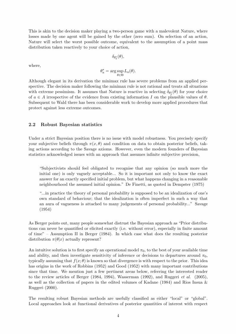
Figure 1: Graphical representation of local-minimax model πsupa,C within a Kullback-Leibler ball

of radius C around the reference model πI , with global (Wald’s) minimax density δθ∗a(θ).

Γ-minimax (for which the Ellsberg paradox is also used as a motivating example, see section 1of Vidakovic (2000)).

Again working in economics, Hansen and Sargent in a series of influential papers (e.g. 2001a,2001b), generalised ideas from Whittle (1990) and Gilboa & Schmeidler (1989) motivated byproblems in macroeconomic time series. They define a robust action as a local-minimax actwithin a Kullback-Leibler (KL) neighbourhood of πI(θ) through exploration of,

ψsup(a) (C) = sup

π∈ΓC

Eπ[La(θ)]

where ΓC denotes a KL ball of radius C around πI ,

ΓC = {π :

∫π(θ) log

(π(θ)

πI(θ)

)dθ ≤ C}.

We will use πsupa,C to denote the corresponding local-minimax distribution,

πsupa,C = arg sup

π∈ΓC

Eπ[La(θ)].

Figure 1 shows a pictorial representation of this constrained minimax rule, where the referencedistribution πI is a point in the spaceM of all distributions on θ (represented by the rectangle)and the least favourable distribution πsup

a,C is contained within the neighbourhood ΓC (representedby the circle of radius C). The Wald minimax distribution is given by δθ∗a(θ). Hansen andSargent showed how πsup

a,C and ψsup(a) can be computed for dynamic linear systems with normal

noise, see Hansen & Sargent (2008) for a thorough review and references.

Breuer & Csiszar (2013a, 2013b), building on the work of Hansen and Sargent, derived cor-responding results for arbitrary probability measures πI(θ). Under mild regularity conditions,and using results from exponential families and large deviation theory they obtain the exactform of πsup

a,C for any πI(θ) given the KL ball of size C, as well as an estimate for ψsup(a) , see also

6

Ahmadi-Javid (2011, 2012). In Section 4 we derive the same result using an alternative, lessgeneral, but perhaps more intuitive proof. Before considering these formal methods we shallstart with exploratory diagnostics and visualisation methods.

3 D-open diagnostics

All good statistical data analysis begins with graphical exploration of information and evaluationof summary statistics before formal modelling takes place. In this section we consider somegraphical displays to aid understanding of when and where actions are sensitive to modellingassumptions. Section 5 further illustrates these ideas. Despite the importance of graphicalstatistics, there are few if any established tools for investigation of decision stability, in contrastto the multitude of methods for investigating model discrepancy and misspecification (Belsleyet al. , 2005; Gelman, 2007; Kerman et al. , 2008). Here we consider three graphical displaysthat concentrate on the relationship between the loss function L(a, θ) and ‘model’ or posteriorπI(θ) for a given a. These are examples of how a set of available actions a ∈ A can be graphicallycompared. They could be displayed as a preliminary step to a formal analysis of sensitivity.

3.1 Value at Risk (Quantile-Loss)

A primary tool for assessing the sensitivity with respect to misspecification of a functional ofinterest, is the distribution of loss, where Za denotes the random loss variable under πI(θ):

FZa(z) = Pr(Za ≤ z) =

∫θ∈Θ

I[La(θ) ≤ z]πI(dθ),

where I[·] is the identity function. We use notation fa(z) = FZa(dz) to denote the correspondingdensity function and F−1

Za(q), for q ∈ [0, 1], is the inverse cumulative distribution or quantile

function. For a given q ∈ [0, 1] it is possible to characterise the value of an action a by its quantileloss or Value at Risk (VaR; terminology used in finance) F−1

Za(1− q). Rostek (2010) developed

an axiomatic framework in which decision-makers can be uniquely characterised by a quantile1−q and rational behaviour (optimal action) is defined as choosing a := arg mina∈A F

−1Za

(1−q).Note that this incorporates the minimax rule by taking q = 0. The author argues that quantilemaximisation is attractive to practitioners as its key characteristic is robustness, specificallyto misspecification in the tails of the loss distribution. Although single quantiles discard muchinformation contained in [πI(θ), La(θ)], plotting this function allows for immediate visualisationof how much of the tails are taken up by high loss (low utility) events. With a bag of samplessimulated from the posterior marginal θ1, .., θm ∼ πI(θ), this is easily approximated:

1. Sort the realised loss values, z(a)i = La(θi), from highest to lowest {z(a)

υa(1) ≥ z(a)υa(2) ≥ . . . ≥

z(a)υ(m)}, where υa(·) defines the sort mapping.

2. For q ∈ [0, 1], approximate F−1Za

(1−q) by linear interpolation of the points(x = k/m, y = z

(a)υa(k)

).

7

3.1.1 Coherent diagnostics

In mathematical finance, summary statistics defined on loss distributions are known as riskmeasures. VaR is a particularly controversial risk measure as it is widely used (written intoofficial regulations, see Basle Committee, 1996) but is not coherent5 (Artzner et al. , 1999)6,violating subadditivity7. This has motivated the use of different diagnostics such as CVaR (seenext section). We note that expected loss and minimax are both coherent diagnostics. However,the use of coherence in Bayesian decision theory does not seem appropriate in general as thesubadditivity axiom does not hold in many applications8.

3.2 Conditional value at risk (upper-trimmed mean utility)

Conditional Value at Risk (CVaR, Rockafellar & Uryasev, 2000) is another popular alternativeto expected loss (or utility), initially motivated by concerns of coherence. To a statistician itrepresents the lower trimmed mean of loss (or upper trimmed mean of utility),

Ga(q) =1

q

∫ ∞F−1Za

(1−q)zfa(z)dz.

This gives the expected value of an action conditional on the event (θ) occurring above a quantileof loss (lowest of utility). q can be seen as regulating the amount of pessimism towards Nature,with limq→0 supaGa(q) corresponding to the minimax rule.

Another strategy for taking in to account model misspecification is by considering the two-sidedtrimmed expected loss, defined as:

H(q) =1

1− q

∫ F−1Za

(1−q/2)

F−1Za

(q/2)zfa(z)dz

This is a robust measure of expected loss formed by discarding events with highest and lowestloss. Both these statistics are easily approximated using the bag of samples {θi}ni=1 and thesort mapping υ defined previously. We use the linear interpolation,

Ga(k

m) =

1

k

k∑i=1

La(θυ(i)), k = 0, ..,m

For a set of actions A, it is possible to quantify the stability of the optimal action a∗ evaluatedunder expected loss, by observing the first CVaR crossing point. That is to say the first valueq ∈ [0, 1] such that a∗ is no longer optimal, evaluated under CVaR(q).

5Note that this is a different definition of coherence from Bayesian coherence, discussed in section 4.1.1.6A coherent risk measure ρ has the following properties: translational invariance: ρ(Z + c) = ρ(Z) + c, where

c is a constant; monotonicity : if Zis stochastically dominated by Y , then ρ(Z) ≤ ρ(Y ); positive homogeneity :ρ(λZ) = λρ(Z), for λ ≥ 0; subadditivity : ρ(Z + Y ) ≤ ρ(Z) + ρ(Y ). By ρ(Z + Y ) we mean the risk measure onthe combined loss distribution of the combination of the two actions corresponding to the loss distributions Zand Y .

7Subadditivity corresponds to investors decreasing risk by diversifying portfolios.8A trivial example is the following: Consider the two gambles, A lose £10 if a fair coin falls on Heads; B lose

£10 if a fair coin falls on Tails. For the same coin, if both gambles are taken then one loses £10 with probability1.

8

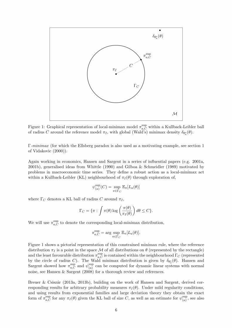
3.3 Cumulative Expected Loss

The Cumulative Expected Loss (CEL) function for action a, defined as,

Ja(q) =

∫ ∞F−1Za

(1−q)zfa(z)dz.

for q ∈ [0, 1]. The CEL-plot is a monotone decreasing function Ja(q) and an informativegraph for highlighting decision sensitivity. The overall shape of Ja(q) provides a qualitativedescription of decision sensitivity. An action with CEL-plot that is steeply rising as q → 0is ‘heavily downside’ (see for example figure 10 in section 5.2), with expected-loss driven bylow-probability high loss outcomes, while CEL-plot rising at 1 indicates ‘heavy upside’. Inparticular Ja(q) has a number of useful features:

• Ja(q) quantifies the contribution to the expected loss of action a, from the 100× (1− q)%set of outcomes with greatest loss.

• Ja(1) = EπI(θ)[La(θ)], is the expected loss of action a, and a = arg maxa∈A Ja(1) is theoptimal Savage action.

• J ′a(q) = infz∗∈R+ {Pr(Za ≤ z∗) = 1− q}, the gradient of the curve at Ja(q) gives thethreshold loss value z∗, such that under action a we can expect with probability (1 − q)the outcome to have loss less than or equal to z∗.This is the “value-at-risk” of action aoutlined above, e.g. Pritsker (1997).

• J ′a(0) = supθ∈Θ La(θ), and hence the Wald minimax action is given by: a = arg mina∈A J′a(0)

(the action with steepest gradient as q → 0).

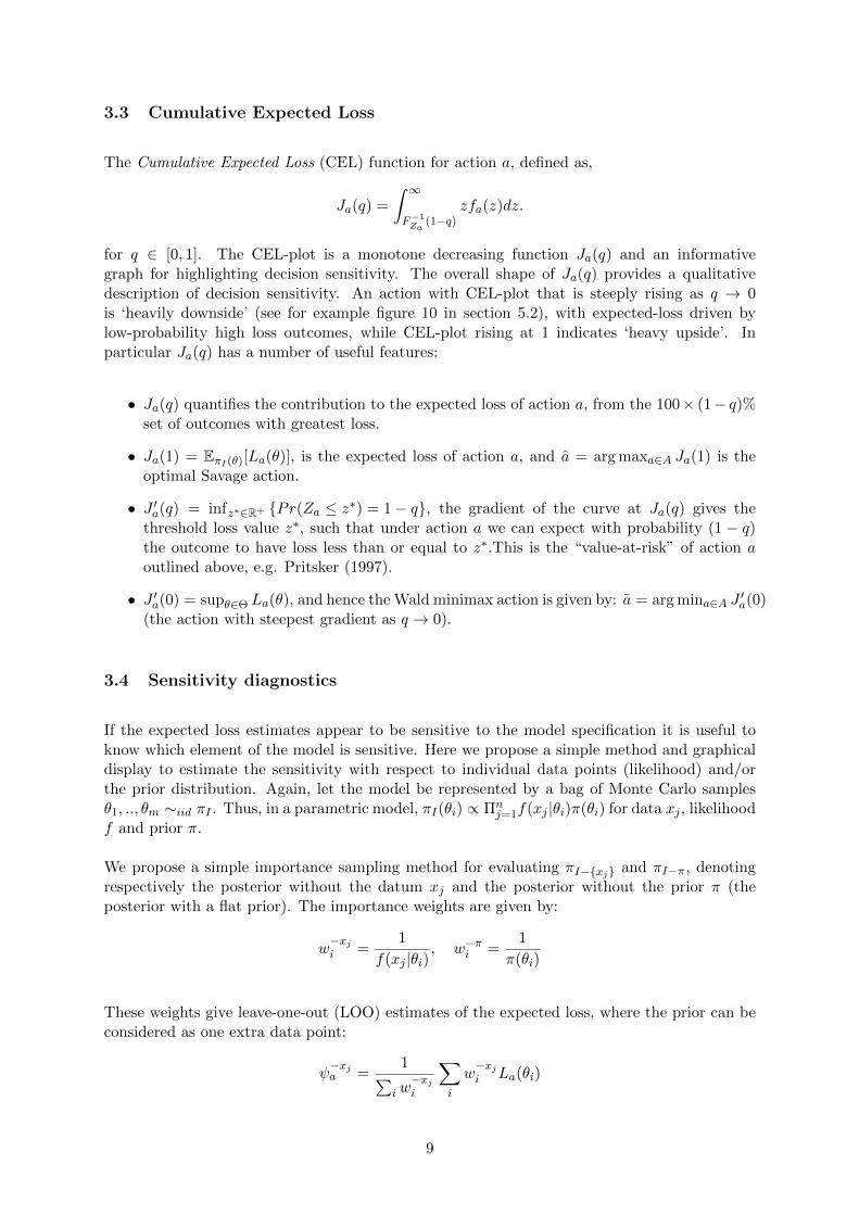
3.4 Sensitivity diagnostics

If the expected loss estimates appear to be sensitive to the model specification it is useful toknow which element of the model is sensitive. Here we propose a simple method and graphicaldisplay to estimate the sensitivity with respect to individual data points (likelihood) and/orthe prior distribution. Again, let the model be represented by a bag of Monte Carlo samplesθ1, .., θm ∼iid πI . Thus, in a parametric model, πI(θi) ∝ Πn

j=1f(xj |θi)π(θi) for data xj , likelihoodf and prior π.

We propose a simple importance sampling method for evaluating πI−{xj} and πI−π, denotingrespectively the posterior without the datum xj and the posterior without the prior π (theposterior with a flat prior). The importance weights are given by:

w−xji =

1

f(xj |θi), w−πi =

1

π(θi)

These weights give leave-one-out (LOO) estimates of the expected loss, where the prior can beconsidered as one extra data point:

ψ−xja =

1∑iw−xji

∑i

w−xji La(θi)

9

0.00

0.01

0.02

0.03

0.04

0.05

−60 −40 −20loss

dens

ity

variable

Status quo

Vaccination

Figure 2: Loss distributions of the two actions with mean values shown by vertical lines.

ψ−πa =1∑iw−πi

∑i

w−πi La(θi)

Thus the effect of single data points can be evaluated (detection of outliers) as can the effect ofthe prior, which is especially useful in small sample situations.

We also propose plotting the loss values La(θi) against the density estimates πI(θi) (up to anormalising constant). This will highlight situations where the high loss samples are comingfrom the tails of the distribution πI .

3.5 Motivating synthetic example

We use an example from the medical decision-making literature to illustrate these three diagnos-tic plots. Consider a certain infectious disease for which there exists treatment medication anda new vaccine. The problem is whether the vaccination should be publicly funded, or whetherthe status-quo should remain in place, whereby patients visit their doctor and are prescribedover the counter drugs. This is a standard setting for decisions made by institutions such asNICE9 in the UK, for example. We use a fictitious example of such a decision process takenfrom Baio & Dawid (2011). The goal is compare the two available actions: widespread vacci-nation or status quo. The modelling must take into account the uncertainty with regards tothe efficacy of the vaccine and its coverage were it to be implemented. With regards the statusquo action, the modelling has to consider the number of visits to the GP10, complications fromthe drugs which could lead to extra visits, possible hospitalisation and even death. Each ofthese outcomes has either a monetary cost (visit to the GP for example) or a utility measuredin Quality Adjusted Life Years (QALYs). Therefore to assign a loss value to each action, it

9National Institute for Clinical Excellence.10General Practitioner

10

0

20

40

60

80

0.00 0.25 0.50 0.75 1.00quantile

Loss

60

65

70

75

80

85

0.00 0.25 0.50 0.75 1.00quantile

Loss

0

20

40

60

0.00 0.25 0.50 0.75 1.00quantile

Loss

57.50

57.75

58.00

58.25

Status quo VaccinationAction

Loss

Figure 3: Diagnostic plots for the decision system given in Baio & Dawid (2011) comparingvaccination (blue) to status quo (red). The ’willingness to pay’ parameter set to 21000. From topleft to bottom right: Inverse loss distribution; Conditional value at risk; Cumulative expectedloss; Expected loss centred at two intervals of standard deviation.

is necessary to choose a conversion rate k, known as the ’willingness to pay’ parameter, ex-changing QALYs into pounds. Most of the decision literature focusses on the sensitivity of thedecision system with respect to the specification of k. The R package BCEA (Bayesian Cost-Effectiveness Analysis) developed by Gianluca Baio implements the model presented in Baio &Dawid (2011) and performs a sensitivity analysis around the parameter k. The exact details ofthe model are not of particular interest so we do not expose them here, our main purpose beingillustrative. The model used for this setting has 28 parameters, each with informative priordistributions, these are given in table 1 of Baio & Dawid (2011). MCMC is used to estimate aposterior distribution, all the relevant details can be found in the package documentation, suchas the cost function used etc. We ran the model given in BCEA using the default settings. Wenote that all the graphs were produced using our package decisionSensitivityR and all the codecan be found in its documentation. In figure 2 we plot the loss distributions for the two actionswith the expected posterior loss values given by the vertical lines. The status quo (red) haslower expected loss but has greater variance than vaccination (blue). The expected loss valuesare very close together, which would suggest sensitivity to model perturbations.

Figure 3 illustrates the three diagnostic plots presented above for this application. We seefrom the inverse loss distribution (top left) that status quo (red) has higher downside loss thanvaccination (blue). The CVaR plot (top right) clearer distinguishes the two actions becauseof this higher downside loss. In this example, the CEL is not informative, but this is contextdependent, see figure 10 from the breast cancer screening application in section 5.2.

The diagnostic plots and summary statistics presented in this section allow for visualisationof dependencies between the loss function and posterior distribution, which can highlight theimpact of model misspecification on decision making. We now look at perturbations to the model(posterior distribution) in order to measure the sensitivity of the expected loss quantities.

11

4 D-open formal methods

A natural approach to ex-post model misspecification is via the construction of a neighbourhoodof ‘close’ models. This allows for either a study of the variation of the quantity of interest(expected loss) ψa over all models in this neighbourhood, or can guide the construction of anonparametric extension of the model. In this section, we explore both ideas, each providingthe statistician with a different set of tools to estimate the sensitivity of the decision system.

For ease of comprehension, all the notation used throughout this paper is summarised in aglossary in Appendix B.

4.1 Kullback-Leibler neighbourhoods

To investigate formally the stability of decisions to model misspecification we suggest follow-ing an approach taken in Hansen & Sargent (2001b) and study the variation of expected lossψ(a) over models within a KL ball Γ around the marginal posterior density, πI(θ), of the ap-proximating model on the states that enter into the loss function. We will assume after lineartransformation that the loss can be bounded, a reasonable assumption for almost all appliedproblems11.

4.1.1 Properties

Analytical form of least favourable distribution It is well known that the KL divergenceis not symmetric, in general KL(π∗||π) 6= KL(π||π∗) for π∗ 6= π, and following others we considerthe neighbourhood ΓC = {π : KL(π||πI) ≤ C}. This might be considered the more naturalsetting as here the KL divergence represents the expected self-information log-loss in using anapproximate model πI when Nature is providing outcomes according to the probability law π.The alternative neighbourhood is considered in the Appendix D. However in the Monte Carlosetting where πI is represented by a set of {θi}mi=1 each with weight 1/m, then any distributionπ that is a reweighing of θi’s satisfies: KL(πI ||π) ≥ KL(π||πI). Because we are looking at thevariation of the expected loss ψ(a) across the ΓC , we want to the neighbourhood to be moreexclusive for fixed values of the radius C.

Surprisingly this situation leads to a least favourable distribution solution with a simple form.

Theorem 4.1. Let πsupa,C = arg supπ∈ΓC Eπ[La(θ)], with ΓC = {π : KL(π ‖ πI) ≤ C} for C ≥ 0.

Then the solution πsupa,C is unique and has the following form,

πsupa,C = Z−1

C πI(θ) exp[λa(C)La(θ)] (2)

where ZC =∫πI(θ) exp[λa(C)La(θ)]dθ is the normalising constant or partition function, for

which we assume ZC <∞, and λa(C) is a non-negative real valued monotone function.

Proof. The function minimisation problem, πsupa,C = arg maxπ∈ΓC Eπ[La(θ)], has an unconstrained

11In practice it is always possible to cap the loss. For instance, any model by which θ is simulated usingMCMC this assumption is made. In finance, the potential losses incurred by any individual or organisation couldbe bounded by an arbitrarily large number, say ±GDP of the US.

12

Lagrange dual form, see for example Hansen et al. (2006) (pages 58-60),

πsupa,C = arg inf

π∈M

{Eπ[−La(θ)] + η−1

a KL(π ‖ πI)}

for some ηa = ηa(C) is a penalisation parameter with ηa ∈ [0,∞), and is monotone increasingin C. Hence,

πsupa,C = arg inf

π∈M

{∫−La(θ)π(θ)dθ + η−1

a

∫π(θ) log

(π(θ)

πI(θ)

)dθ

}= arg inf

π∈M

{∫π(θ) log

(π(θ)

πI(θ) exp[ηaLa(θ)]

)dθ

}∝ πI(θ) exp[ηaLa(θ)] (3)

The uniqueness arises from the convexity of the KL loss. The result follows, taking λa(C) =ηa.

By a similar argument the distribution of minimum expected loss follows:

πinfa,C ∝ πI(θ) exp[−λ(C)La(θ)]

Note by assuming bounded loss functions we can ensure the integrability of the densities. Breuer& Csiszar (2013a) and Ahmadi-Javid (2012) derive the same result more generally but perhapsless intuitively. Breuer & Csiszar (2013a) gives more general conditions on when the solutionexists.

The ΓC least favourable distributions, {πinfa,C , π

supa,C}, have an interpretable form as exponentially

tilted densities, tilted toward the exponentiated loss function, with weighting λa(C) a monotonefunction of the neighbourhood size C. For linear loss, La(θ) = Aθ, the local least favourableπsupa,C is the well known Esscher Transform used for option pricing in actuarial science. The

tilting parameter λa(C) is a function of the neighbourhood size C, but we will write λa forconvenience. λa and C can be thought of as interchangeable, as there is a bijective mappingbetween C ≥ 0 and λa ≥ 0, although this is not a linear mapping.

Following Theorem 4.1, the corresponding range of expected losses for each action (ψinf(a), ψ

sup(a) )

can then be plotted as a function of C for each potential action. Formally we should write[ψinf

(a)(C), ψsup(a) (C)] although for ease of notation we will often suppress C from the expression

unless clarity dictates. The constraint KL(π ‖ πI) ≤ C will result in πsupa,C lodging on the

boundary as the expected loss can always be increased by diverging toward δθ∗a(θ) for anydistribution with KL(π ‖ πI) < C. Substituting the solution (2) into the KL divergencefunction gives,

KL(πsupa,C ‖ πI) =

∫πsupa,C(θ) log

(Z−1λa

exp[λaLa(θ)])dθ

= λaEπsupa,C

[La(θ)]− logZλa

So, given neighbourhood size C, the KL divergence KL(πsupa,C ‖ πI) is λa(C) times the expected

loss under πsupa,C minus the log partition function. Moreover, by Jensen’s inequality,

KL(πsupa,C ‖ πI) = λaEπsup

a,C[La(θ)]− logEπI [exp(λaLa(θ)]

≤ λa

[Eπsup

a,C[La(θ)]− EπI [La(θ)]

]

13

The KL divergence is bounded above by λa times the difference in expected loss between theapproximating and the contained minimax models.

By plotting out the interval [ψinf(a)(C), ψsup

(a) (C)] for each action as a function of KL divergence

constraint C : KL(π ‖ πI) ≤ C we can look for crossing points between the supremum loss ψsup(a)

under the optimal action a chosen by the approximating model and the infimum loss under allother actions, ψinf := infa∈A\a{ψinf

(a)}

Bayesian coherence Adapting results from Bissiri et al. (2013), we are are able to state thefollowing result regarding the uniqueness of Kullback-Leibler divergence under the condition ofguaranteeing coherent Bayesian updating.

Theorem 4.2. Let πsupa,C(x, πI) be the solution obtained by

πsupa,C(x, πI) = arg inf

π∈M

{Eπ[−La(θ)] + η−1

a D(π ‖ πI)}

with data x = {xi}ni=1, a centring distribution πI , and arbitrary g-divergence measure D. More-over, let x be partitioned as x = {x(1), x(2)}, for x(1) = {xi}i∈S, x(2) = {xj}j∈S, where S, S isany partition of the indices i = 1, .., n. For coherence we require,

πsupa,C(x, πI) ≡ πsup

a,C

(x(2), πsup

a,C(x(1), πI))

That is, the solution using a partial update involving x(1), which is subsequently updated withx(2), should coincide with the solution obtained using all of the data, for any partition. Thenfor coherence D(·||·) is the Kullback-Leibler divergence.

The proof is given in Appendix A.

This theorem shows that KL is the only divergence measure to provide coherent updating ofthe local least favourable distribution.

Local sensitivity: Although the framework presented here fits into global robustness meth-ods, it is also possible to use it to extract local robustness measures. In appendix C we show thatthe derivative at zero of least favourable expected loss w.r.t. λ (exponential tilting parameter)is exactly the variance of the loss distribution. This justifies the use of the variance of loss as alocal sensitivity diagnostic.

Local Bayesian admissibility In a classical setting, the notion of admissibility helps definea smaller class of actions that can then be further scrutinized in order to choose an optimaldecision. A decision is denoted inadmissible if there does not exist a θ such that its riskfunction (frequentist) is minimal (with respect to the other decisions) at θ. We note that in aBayesian context, because the expected loss is a single quantity used to classify actions, only theaction which minimizes expected loss is admissible. However if we consider the set of posteriordistributions contained within a Kullback-Leibler neighbourhood of radius C, then an analogousdefinition of admissibility can be given.

First we define the pairwise difference in expected losses of any two actions (a, a′) ∈ A, the‘regret’ loss of having chosen a instead of a′:

L(a,a′)(θ) = La(θ)− La′(θ)

14

and the corresponding least favourable pairwise distribution:

πsup(a,a′),C = arg sup

π∈ΓC

{Eπ[L(a,a′)(θ)]

}= Z−1

C πI(θ) exp(λ(a,a′)[La(θ)− La′(θ)]

)with expected loss ψsup

(a,a′)(C) =∫θ π

sup(a,a′),C(θ)[La(θ)− La′(θ)]dθ.

Definition 1. We say that an action a is C∗-dominated, or locally-inadmissible up to level C∗

when,C∗ := arg sup{C : ψsup

(a,a′)(C) < 0, ∀a′ ∈ A \ a}

If a is∞-dominated then it is globally inadmissible (this retrieves the classical notion of admis-sibility).

We note that plotting ψsup(a) (C), a ∈ A for values C ∈ [0, C∗] does not give any information

as to the admissibility of the actions a ∈ A. In order to graphically represent admissibility(inadmissibility), it is necessary to look at least favourable distributions defined over the pairwisedifference in loss for two actions a, a′. By plotting ψsup

(a,a′) as a function of constraint radius Cwe can look for actions that are dominated, such that there is no π ∈ ΓC for which they areoptimal.

Calibration of neighbourhoods In most scenarios the local least favourable distributionZ−1λ πI(θ) exp[λaLa(θ)] will not have closed form. Moreover πI(θ) will often only be represented

as a Monte Carlo bag of samples {θi}mi=1 ∼iid πI . In this case the distribution can be approxi-mated by using πI as an importance sampler (IS) leading to,

πsupa,C =

1

Zλa

∑i

wiδθi(θ)

wi = exp[λaLa(θi)], Zλa =∑i

wi

We can then use πsupa,C to calculate (ψinf

(a), ψsup(a) ). For a small neighbourhood size and hence small

λa relative to La(θ) this IS approximation should be reasonable. In general if πI is thought tobe a useful model to the truth then the neighbourhood size should be kept small. However asλ increases, the variance of the un-normalised importance weights will grow exponentially andthe approximation error with it. In this situation the problem appears amenable to sequentialMonte Carlo samplers taking λa ≥ 0 as the “time index” although here we do not explore thisany further. This points to the wider issue of how to choose the size of the neighbourhood Γ.However, in the Monte Carlo setting of this problem, the statistician can decide on candidateKL values using one or more of the following ideas:

• Plotting the distribution of the importance weights and deciding whether this is ‘degen-erate’. By this we mean all the mass on one or more samples with high loss, and no masson the lower values. This can be summarised by the variance of the weights, with theminimax solution having variance (m− 1)/m2.

• Define a inequality score for the set of importance weights. All weights wi = 1/m wouldbe perfectly equal, and the minimax solution would be perfectly unequal. We suggestconsidering KL values C up to a Cmax defined as assigning 99% of the mass to 1% of thesamples.

15

• Use qualitative exploratory methods. For example, plot the marginal distributions of theminimax solution over dimensions of interest, i.e. which are interpretable.

We consider that the calibration of the Kullback-Leibler divergence remains an open problem,even though this divergence is used in many applications. McCulloch (1989) proposes a generalsolution using a Bernoulli distribution, but it is not obvious that this translates well into amethod for the calibration of any continuous distribution.

4.1.2 Connections to other work

The use of local least favourable distributions turns out to be connected to well known statisticaltechniques. We outline some examples for illustration.

Predictive tempering as a local least favourable distribution Consider the task, or

action, to provide a predictive distribution, f(y|x), for a future observation y given covariatesx. The local proper scoring rule in this case is known to be the self-information logarithmic lossL(y) = − log f(y|x) Bernardo & Smith (1994). The conventional Bayesian solution is to report

your honest marginal beliefs as f(y|x) = fI(y|x), where given a model parametrised by θ wehave fI(y|x) =

∫f(y|x, θ)πI(θ)dθ. However this assumes that the model is true and moreover

that the prediction problem is stable in time, in that the prediction probability contours donot drift (see below). Both of these assumptions may be dubious. The robust local-minimaxsolution above protects against misspecification and leads to

f∗sup(y|x) ∝ fI(y|x)1−λ,

for λ ∈ [0, 1]. This has the form of tempering the predictive distribution, taking into accountadditional external levels of uncertainty outside of the modelling framework. In this way, pre-dictive annealing can be seen as a local-minimax action.

Concept drift. In data mining applications we may have access to meta-data, ti, for thei’th observation and a belief that loss is ordered or structured by the information in t. Forexample, t might index time and due to “concept drift” the analysis might hold greater loss inpredicting using more historic collected observations, (e.g. Section 3.1 in Hand, 2006), thoughmore generally ti simply contains information relative to predictive loss. In this case the naturalloss function is a weighted self-information loss, based on the empirical distribution:

L(θ) = −∑i

∆(ti) log f(yi; θ).

with ∆(ti) ∈ (0, 1) encapsulating the relative weight of log loss to the future predictive.

For prediction of a new observation y∗ given x∗ this leads to the robust solution as

fsup(y∗|x∗) ∝∫θf(y∗|x∗, θ)

[∏i

f(yi; θ)π(θ)]

]e−

∑i ∆(ti) log f(yi;θ)dθ

∝∫θf(y∗|x∗, θ)

[∏i

f(yi; θ)1−∆(ti)π(θ)

]dθ

16

that can be seen to down-weight the information in yi used to predict y∗. For example, if tirecords the time since the current prediction time then a natural penalty is ∆(ti) = exp(−λti),where λ encodes a predictive forgetting factor. For a related approach see Hastie & Tibshirani(1993).

Gibbs Posteriors and PAC-Bayesian: Suppose you hold prior beliefs about a set of pa-rameters θ but don’t know how to specify the likelihood f(x|θ), and hence lack a model π(x, θ).For example, suppose θ refers to the median of FX with unknown distribution. Suppose thetask (action) is to provide your best subjective beliefs π(θ|·) conditional on information in thedata and prior knowledge. We don’t have a likelihood but we could have a well defined priorhence πI(θ) = π(θ). In this situation there may be a well defined loss function on the data thatwe would wish to maximise utility against for specifying beliefs, e.g. for the median we shouldtake

L(θ) =∑i

|xi − θ|

The distribution that minimises the expected loss within a certain KL divergence of the prioris given by the local-maximin distribution,

πinfa,C = Z−1

λae−λa

∑i |xi−θ|π(θ)

This has the form of a Gibbs Posterior or an exponentially weighted PAC-Bayesian approach(Zhang, 2006a,b; Bissiri et al. , 2013; Dalalyan & Tsybakov, 2008, 2012). In this way wecan interpret Gibbs posteriors as local-maximin solutions in the absence of a known samplingdistribution (Bissiri et al. , 2013).

Conditional Γ-minimax priors: There is a direct relationship to Γ-minimax priors whenthe La(θ) involves all the parameters in a parametric model where the posterior is

πI(θ) ∝ Πnj=1f(xj |θ)π(θ)

with likelihood f(·|θ) and prior π(θ).

Thus the posterior least favourable distribution

πsupa (θ) ∝ eλaLa(θ)Πn

j=1f(xj |θ)π(θ)

can be considered a Bayes update using the minimax prior eλaLa(θ)π(θ) (dropping the normali-sation constant). This is an action specific prior.

Note that the KL divergence is the only divergence to ensure this coherency, and also that the“prior” πsup

a (θ) is data dependent if the loss function uses the empirical risk, i.e. is of the formLa(θ,X).

4.2 Weak Neighbourhoods

From a Bayesian standpoint its more natural to characterise the variation in expected lossarising over all models in some neighbourhood Γ, rather than performing minimax optimisationwithin the neighbourhood. In order to quantify this uncertainty and take expectations overdistributions in the neighbourhood of πI , we require a probability distribution on a set of

17

probability measures centred on πI . This is classically a problem in Bayesian nonparametrics, seefor example Hjort et al. (2010). However, in a decision-theoretic context, only the functionalsof the distributions π ∈ Γ are of importance. In particular the functionals ψa : π → Eπ[La(θ)]for a ∈ A (expected loss). It is important to note that two sequences of distributions πn, π

∗n can

be infinitely divergent in Kullback-Leibler, or can remain at a finite distance in total variationmetric, but weakly converge, i.e. their functionals converge, see Watson et al. (2014) for anexample and a further discussion of this. Thus, if we set a nonparametric distribution Π overmeasures π, that is centred at πI : instead of studying the ’distance’ between draws π ∼ Πand the reference distribution πI , we can study the distance between the induced distributionsFa,π(z) and Fa,πI (z), the (cumulative) distributions of loss for action a. A suitable candidatedistribution Π should have wide support (to overcome the possible misspecification) and itshould be possible to characterise the distance of the induced distributions Fa,π. The DirichletProcess (DP) allows for exactly such a construction.

4.2.1 Dirichlet Processes for functional neighbourhoods

Definition 2. Dirichlet Process: Given a state space X we say that a random measure Pis a Dirichlet Process on X , P ∼ DP (α, P0), with concentration parameter α and baselinemeasure P0 if for every finite measurable partition {B1, . . . , Bk} of X , the joint distribution of{P (B1), . . . , P (Bk)} is a k-dimensional Dirichlet distribution Dirk{αP0(B1), . . . , αP0(Bk)}.

Using this definition we can then sample from distributions in the neighbourhood of πI accordingto π ∼ DP (α, πI), for some α > 0. In practice we can consider a draw from the DP via aconstructive definition,

{θi}mi=1 ∼ πIw ∼ Dirm(α/m, . . . , α/m),

π(θ) :=m∑i=1

wiδθi(θ)

(4)

where the θi’s are i.i.d. from πI and independent of the Dirichlet weights. As m→∞, π tendsto a draw π ∼ DP (α, πI). This construction fits well with the Monte Carlo context, where πI isrepresented by a bag of samples {θi}mi=1. If we draw multiple vectors w(1), .., w(k) ∼ Dirm, thenin the limit m→∞, each corresponds to an independent draw from the DP (α, πI), conditionalon the atoms θi. In an ideal world, we would want to resample a set {θi}mi=1 at each step. Butthis would not be feasible in practice and would defeat our purpose of constructing an ex-postmethodology for analysing sensitivity. Therefore, this construction of the Dirichlet Process ismore adapted than say the stick-breaking representation.

For an action a, the expected loss under the re-weighed draw π is given by:

ψπa =∑i

wiLa(θi) (5)

and the loss distribution by:

Fa,π(z) =∑i

wi1z≤La(θi)(z)

In what follows, without loss of generality, we fix a and consider the θi to be ordered by loss, i.e.La(θ1) ≤ ... ≤ La(θm). Let vi =

∑ij=1wi, the cumulative summed weights, and xi := i/m for

18

i = 1, ..,m. We also consider that the loss function L(a, θ) has undergone the following lineartransformation (which does not alter the ranking of actions under expected loss):

L(a, θ)→L(a, θ)−mina,θ L(a, θ)

maxa,θ L(a, θ)−mina,θ L(a, θ)(6)

This means each loss cdf takes values between [0,1]. We can study the L1 distance between theempirical distribution12 Fa,πI and the reweighed version Fa,π which is given by:

m∑i=1

|vi − xi| · [La(θi)− La(θi−1)]

For a fixed sample {θi}mi=1, the increments La(θi) − La(θi−1) are also fixed, and it is possibleto compute the expected difference |vi − xi| by noting that vi ∼ Beta(xiα, (1 − xi)α). This isgiven by:

Ev{|vi − xi|} =2

α

[xxii (1− xi)(1−xi)]α

Beta(xiα, (1− xi)α)

As a consequence of the linear transformation given in (6), this L1 difference is bounded by1/2. Ew{|Fa,π−Fa,πI |} is dependent on the concentration parameter α which controls how closethe draws Fa,π are from the reference loss distribution; increasing α shrinks the L1 distance.However, it is important the note that this distance will also be dependent on the form of theloss function, i.e the increments La(θi)− La(θi−1).

4.2.2 Probability of optimality

From properties of the Dirichlet Process, we know that EΠ[La(θ)] = EπI [La(θ)], where Π isthe nonparametric measure defined in equation (4). Thus if an action a is optimal under thecriterion of posterior expected loss (taken with respect to πI), it will remain optimal underexpected loss taken with respect to Π. Instead of looking at expected loss we consider theprobability that a particular action will be optimal when drawing a random π ∼ DP (πI , α)(and computing expected loss with respect to this random π). That is to say, each randomdraw π will induce a distribution of loss Fa,π for action a. The probability that a is optimalwill depend on the concentration parameter α. As the concentration parameter α → ∞, therandom loss distribution Fa,π tends to Fa,πI in probability under the L1 norm, thus givingback the optimality mapping induced by πI . This gives rise to a diagnostic graph, where theprobability of optimality of each action is plotted against the parameter α. The probability ofoptimality is non-analytical in the general case, and dependent on the form of the loss functionL(a, θ). However, given a Monte Carlo representation of πI and thus a matrix of loss values(number of samples θi times number of actions) it is easy to approximate via successive drawsw ∼ Dir(α/n, .., α/n) and using the construction given in (5).

4.2.3 Calibration of the Dirichlet Process extension

Contrary to the methodology proposed in section 4.1, using a Dirichlet Process as a nonparamet-ric model extension to test robustness gives a framework which is not action specific. However,it also relies on a free parameter α which needs to be calibrated in a principled manner. In

12empirical in the sense that it corresponds to πI through i.i.d. sampling.

19

0.00

0.25

0.50

0.75

1.00

0.00 0.25 0.50 0.75 1.00quantile

Loss

log10(α)

0

1

2

3

4

Figure 4: 95% confidence intervals around the reference action a∗ for different values of theconcentration parameter α. From widest to tightest: log10(α) values are 0,1,2,3,4.

order to do this, we define a reference action a∗, such that the loss distribution is given byFa∗,π(z) = z, for z ∈ [0, 1]13.

With the construction given in (5), if we draw weights w ∼ Dirm(α/m, . . . , α/m) and useuniform loss intervals, i.e. reweighing the distribution Fa∗,π(z), it is then possible to compute95% confidence intervals for draws from a Dirichlet Process for a specific value of the parameterα. Figure 4 shows an approximation of these confidence intervals for a series of values α whoselog10 values are integers from 0 to 4. It is clear that low values of α (between 0 and 10 forexample) imply a very low trust in the model, as the draws can vary hugely from the referencedistribution. However the statistician might want the decisions to be robust to higher values ofα where the draws are much tighter. In section 5.2 we illustrate the use of this method.

5 Applications

5.1 Synthetic Example, continued

To illustrate the ideas from sections 4.1 and 4.2, we continue with the vaccination vs. status quodecision problem given in section 3.5. Figure 5 plots the expected loss of each action under thelocal least favourable distribution, as a function of the size C of the KL ball14. We observe thatfor very small value of KL the status quo action is no longer optimal. This is because of its muchhigher variance of loss. However, figure 6 shows the probability of optimality for each action asa function of the concentration parameter α (log scale). This highlights that in fact, the systemis decision robust (see section 6 for a discussion on decision robustness vs. loss robustness)The vaccination vs. status quo decision problem is synthetic but it allows us the illustrate the

13After the linear transformation given in (6).14Using the function preliminaryAnalysis from our package decisionSensitivityR

20

−32

−30

−28

−26

−24

0.00 0.05 0.10 0.15 0.20 0.25KL

Exp

ecte

d lo

ss

Local minimax loss

−2.0

−1.5

−1.0

−0.5

0.0

0.00 0.05 0.10 0.15 0.20 0.25KL

Exp

ecte

d Lo

ss

Difference in minimax loss

Figure 5: Diagnostic plots for the local least favourable distribution, comparing vaccination(blue) to status quo (red). Top: local least favourable expected loss; Bottom: difference inminimax between non optimal and optimal actions.

0.00

0.25

0.50

0.75

1.00

0 1 2 3log(α)

Pro

babi

lity

Figure 6: Probability of optimality of the two actions (red: status quo, blue: vaccination) undera nonparametric extended model using a DP (πI , α). The α-values are plotted on a log scale.

21

A B

D

CtB ∼ f(t|µ, σ2) tC ∼ q(t|κ, ρ, tB)

tD ∼ h(t|α, β, tB , tC)tD ∼ h(t|α, β)

tD ∼ h(t|α, β, tB)

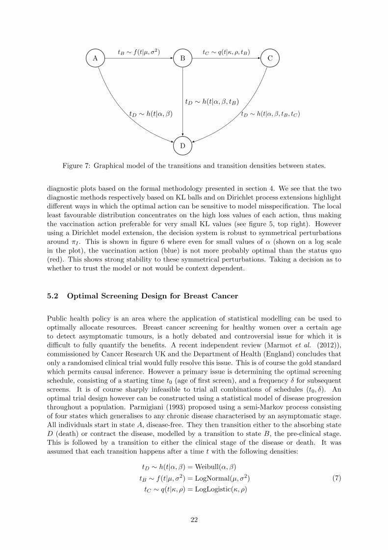
Figure 7: Graphical model of the transitions and transition densities between states.

diagnostic plots based on the formal methodology presented in section 4. We see that the twodiagnostic methods respectively based on KL balls and on Dirichlet process extensions highlightdifferent ways in which the optimal action can be sensitive to model misspecification. The localleast favourable distribution concentrates on the high loss values of each action, thus makingthe vaccination action preferable for very small KL values (see figure 5, top right). Howeverusing a Dirichlet model extension, the decision system is robust to symmetrical perturbationsaround πI . This is shown in figure 6 where even for small values of α (shown on a log scalein the plot), the vaccination action (blue) is not more probably optimal than the status quo(red). This shows strong stability to these symmetrical perturbations. Taking a decision as towhether to trust the model or not would be context dependent.

5.2 Optimal Screening Design for Breast Cancer

Public health policy is an area where the application of statistical modelling can be used tooptimally allocate resources. Breast cancer screening for healthy women over a certain ageto detect asymptomatic tumours, is a hotly debated and controversial issue for which it isdifficult to fully quantify the benefits. A recent independent review (Marmot et al. (2012)),commissioned by Cancer Research UK and the Department of Health (England) concludes thatonly a randomised clinical trial would fully resolve this issue. This is of course the gold standardwhich permits causal inference. However a primary issue is determining the optimal screeningschedule, consisting of a starting time t0 (age of first screen), and a frequency δ for subsequentscreens. It is of course sharply infeasible to trial all combinations of schedules (t0, δ). Anoptimal trial design however can be constructed using a statistical model of disease progressionthroughout a population. Parmigiani (1993) proposed using a semi-Markov process consistingof four states which generalises to any chronic disease characterised by an asymptomatic stage.All individuals start in state A, disease-free. They then transition either to the absorbing stateD (death) or contract the disease, modelled by a transition to state B, the pre-clinical stage.This is followed by a transition to either the clinical stage of the disease or death. It wasassumed that each transition happens after a time t with the following densities:

tD ∼ h(t|α, β) = Weibull(α, β)

tB ∼ f(t|µ, σ2) = LogNormal(µ, σ2)

tC ∼ q(t|κ, ρ) = LogLogistic(κ, ρ)

(7)

22

Figure 7 shows a graphical model of the four state semi-Markov process with transition densities.An individual is characterised by the triple t = (tB, tC , tD) where the symptomatic stage of thedisease is contracted only when tD < tB + tC (assuming that all individuals will contract thedisease if they lived long enough). For a screening schedule a = (t0, δ) the loss function isdefined as follows (a function of the times t = (tB, tC , tD)):

L(a, t) = r · na(t) + 1C (8)

0.00

0.01

0.02

0.03

25 50 75 100age

dens

ity

0.0

0.2

0.4

0.0 2.5 5.0 7.5 10.0age

dens

ity

0.00

0.01

0.02

0.03

20 40 60 80 100age

dens

ity

Figure 8: Probabilistic model of transition times: (from top to bottom) marginal densitiesof transition times to preclinical stage, transition from preclinical to clinical stage, and deathtimes.

where na is the number of screening schedules an individual will receive during their lifetime,until they die or enter into the asymptomatic stage of the disease. 1C is the indicator function,taking value 1 for the event that the pre-clinical tumour is not detected by screening or occursbefore t0, and zero otherwise. r trades off the cost of one screen against the cost incurred bythe onset of the clinical disease. Each screen has an age-dependent false-negative rate modelledwith a logistic function:

β(t) =1

1 + e−bo−b1(t−t)

where t is the average age at entry in the study group. To simulate transition times for indi-viduals from this model, we used 2000 posterior parameter samples for θ = (µ, σ2, κ, ρ, b0, b1)given in the supplementary materials of Wu et al. (2007). This is based on data from the HIPstudy Shapiro et al. (1988). Figure 8 shows the estimated marginal densities for 104 sampledtimes for each transition event15. To carry out an ex-post analysis of this model, we first con-sidered 32 alternative schedules, consisting of all combinations of starting ages taken from theset {55, 57, 59, 61, 63, 65, 67, 69} (years) and screening frequencies of {9, 12, 15, 18, 24} (months).This choice of screening schedules is mainly illustrative for our purposes: the optimal schedulewill heavily depend on the choice of r (trade-off ratio in equation 8) which we do not attemptto justify (the value 10−3 was taken from the section 4.5 of Ruggeri et al. (2005) where the au-thors also considered this application). In order for the plots to be legible, we selected the top 6schedules 16(as ordered by expected loss under the reference model) for analysis. However, there

15We calibrate the Weibull distribution with values α = 7.233, β = 82.651 which are the values used inParmigiani (1993)

16Given in order of increasing expected loss these are: (59,15), (55,15), (57,15), (61,15), (55,18) and (59,18).

23

0

5

10

15

20

25

0.00 0.25 0.50 0.75 1.00loss

dens

ity

0

5

10

15

20

25

0.00 0.25 0.50 0.75 1.00loss

dens

ity

0

5

10

15

20

0.00 0.25 0.50 0.75 1.00loss

dens

ity

0

5

10

15

20

0.00 0.25 0.50 0.75 1.00loss

dens

ity

Figure 9: Top left: loss density for the optimal action (start at 59, frequency 15 months) underthe approximating model πI given in (7). Going from top right to bottom right: loss densities,for the same action, under the local least favourable distribution at KL divergences equivalentto a reassignment of mass of 2, 5 and 10%, respectively. These are approximate: 0.008, 0.08,0.3. The effect can be seen as increasing the mass put onto high loss events.

is no reason not to analyse a greater number of schedules other than for clarity in plotting. Thetop left plot in figure 9 shows the loss density plot of the optimal action corresponding to theschedule a = (t0 = 59, δ = 15) (units in years and months) and a trade-off parameter r = 10−3.The other three plots show the corresponding loss density for the minimax distributions at KLvalues equivalent to reassigning 2,5 and 10% of the mass, respectively. The effect can be see astransferring the mass from left to right, i.e. from low loss to high loss. The losses incurred fora particular schedule a = (t0, δ) can be seen to be highly bimodal. Most of the population donot contract the disease and therefore contribute a loss of r ·na (cost of screen times number oftotal screens during lifetime ). The loss contributed by those who do contract the clinical stageof the disease is of magnitude 1/r greater by definition.

Figure 10 gives four diagnostic plots for the loss distribution: inverse loss distribution, theValue at Risk, the Conditional Value at Risk and the Conditional Expected Loss. These aredefined in section 3 and are shown here with the schedules (decisions) aforementioned. TheConditional Expected Loss plot very clearly shows that the expected loss values are driven bylow probability events (around 10% of the mass).

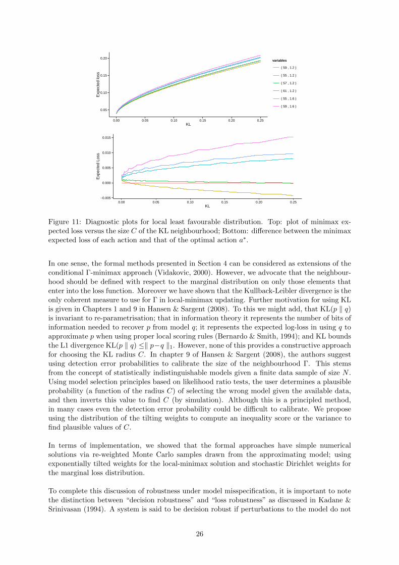
The diagnostic plot in figure 11 which based on the theory given in section 4.1 confirms thatthe decision system is sensitive to small changes in the model. The difference in expected lossunder the local least favourable distributions between action (55,15) and the optimal actionis negative for small KL values (bottom plot, figure 11). Hence small perturbations (in KLdivergence) changes the optimality of the actions. This is also apparent from figure 12, wherewe plot the local admissibility of the optimal action under πI (see section 4.1.1. For very smallneighbourhoods of in KL, the optimal Bayes action is no longer locally admissible.

As a final diagnostic plot we look at the probability of optimality under the Dirichlet exten-

24

0.00

0.25

0.50

0.75

1.00

0.00 0.25 0.50 0.75 1.00quantile

Loss

0.00

0.25

0.50

0.75

1.00

0.00 0.25 0.50 0.75 1.00quantile

Loss

0.00

0.01

0.02

0.03

0.00 0.25 0.50 0.75 1.00quantile

Loss

0.035

0.036

0.037

0.038

( 55 , 1.2 ) ( 55 , 1.6 ) ( 57 , 1.2 ) ( 59 , 1.2 ) ( 59 , 1.6 ) ( 61 , 1.2 )Action

Loss

Figure 10: Model diagnostic plots. From top left to bottom right: inverse loss distributionsof the 6 actions (all very close in shape); Upper trimmed mean loss which differentiates theactions by showing the higher downside in some schedules; conditional expected loss; estimatesof expected loss centred inside intervals of two standard deviations. We see that the expectedloss ψa,πI for all actions is driven by low probability, high loss events (shape of CEL plot).

sion model (section 4.2). Figure 13 shows the probability for varying values of concentrationparameter α of each action being optimal. We see that for large values of α (greater than 104)we recover the optimal action under πI . However, for smaller values, the least optimal underπI (of the 6 selected) has a higher probability of being optimal. This shows the lack of decisionrobustness in this problem, mainly due to flatness of the loss surface.

This application highlights an interesting distinction that must be made when considering modelmisspecification in a decision-theoretic context. The loss surface is very flat for changes inscreening schedule. That is to say, there is little relative difference in expected loss betweensimilar screening schedules. This is also noted by Ruggeri et al. (2005) in their analysis of theproblem. This particular application is robust to changes in the model (in an expected losssense) but not however decision robust. I.e. small perturbations to the model will change theoptimality of an action a∗. We discuss this idea further in section 6.

6 Conclusions

The goal of this article is to aid decision makers by providing statistical methods for exploringsensitivity to model misspecification. We hope this will generate further debate and researchin this field. The increase in complex high-dimensional data analysis problems, “big-data”, hasdriven a corresponding rise in approximate probabilistic techniques. This merits a reappraisalof existing diagnostics and formal methods for characterising the stability of inference to knownapproximations.

25

0.05

0.10

0.15

0.20

0.00 0.05 0.10 0.15 0.20 0.25KL

Exp

ecte

d lo

ss

variables

( 59 , 1.2 )

( 55 , 1.2 )

( 57 , 1.2 )

( 61 , 1.2 )

( 55 , 1.6 )

( 59 , 1.6 )

−0.005

0.000

0.005

0.010

0.015

0.00 0.05 0.10 0.15 0.20 0.25KL

Exp

ecte

d Lo

ss

Figure 11: Diagnostic plots for local least favourable distribution. Top: plot of minimax ex-pected loss versus the size C of the KL neighbourhood; Bottom: difference between the minimaxexpected loss of each action and that of the optimal action a∗.

In one sense, the formal methods presented in Section 4 can be considered as extensions of theconditional Γ-minimax approach (Vidakovic, 2000). However, we advocate that the neighbour-hood should be defined with respect to the marginal distribution on only those elements thatenter into the loss function. Moreover we have shown that the Kullback-Leibler divergence is theonly coherent measure to use for Γ in local-minimax updating. Further motivation for using KLis given in Chapters 1 and 9 in Hansen & Sargent (2008). To this we might add, that KL(p ‖ q)is invariant to re-parametrisation; that in information theory it represents the number of bits ofinformation needed to recover p from model q; it represents the expected log-loss in using q toapproximate p when using proper local scoring rules (Bernardo & Smith, 1994); and KL boundsthe L1 divergence KL(p ‖ q) ≤‖ p−q ‖1. However, none of this provides a constructive approachfor choosing the KL radius C. In chapter 9 of Hansen & Sargent (2008), the authors suggestusing detection error probabilities to calibrate the size of the neighbourhood Γ. This stemsfrom the concept of statistically indistinguishable models given a finite data sample of size N .Using model selection principles based on likelihood ratio tests, the user determines a plausibleprobability (a function of the radius C) of selecting the wrong model given the available data,and then inverts this value to find C (by simulation). Although this is a principled method,in many cases even the detection error probability could be difficult to calibrate. We proposeusing the distribution of the tilting weights to compute an inequality score or the variance tofind plausible values of C.

In terms of implementation, we showed that the formal approaches have simple numericalsolutions via re-weighted Monte Carlo samples drawn from the approximating model; usingexponentially tilted weights for the local-minimax solution and stochastic Dirichlet weights forthe marginal loss distribution.

To complete this discussion of robustness under model misspecification, it is important to notethe distinction between “decision robustness” and “loss robustness” as discussed in Kadane &Srinivasan (1994). A system is said to be decision robust if perturbations to the model do not

26

0.0000

0.0025

0.0050

0.0075

0.0000 0.0025 0.0050 0.0075 0.0100

variable

1

2

3

4

5

Figure 12: Local Bayesian admissibility plot.

effect the optimality of an action a. On the other hand, it is said to be loss robust, if thoseperturbations do not effect the overall expected loss of the action a (in a relative sense). It isclear that a decision system can have one property without the other. Which is more desirablewill be highly context dependent. Throughout the article we have taken the loss function to beknown. However, it is clear that loss misspecification is also an important element of robustdecision making. Further work is needed to develop a unified approach for dealing with this. Ourframework ignores misspecification in the loss function. Certain loss functions are often chosenfor computational ease or because they posses other desirable properties such as convexity. Also,elicitation of the true loss function can be difficult (for an example see the application discussedin section 5.2). Hence for completeness, a robustness analysis of a decision system must takethis into account. Ruggeri et al. (2005) (pages 636-639) provides some further discussion andreferences.

Acknowledgements

We thank Luis Nieto-Barajas, George Nicholson and Tristan Gray-Davies for many helpfuldiscussions and suggestions. Watson was supported by an EPRSC grant from the IndustrialDoctorate Centre (SABS-IDC) at Oxford University and by Hoffman-La Roche. Holmes grate-fully acknowledges support for this research from the Oxford-Man Institute, the EPSRC, theMedical Research Council and the Wellcome Trust.

27

0.00

0.25

0.50

0.75

1.00

0 1 2 3 4log(α)

Pro

babi

lity

variable

( 59 , 1.2 )

( 55 , 1.2 )

( 57 , 1.2 )

( 61 , 1.2 )

( 55 , 1.6 )

( 59 , 1.6 )

Figure 13: Probability of being optimal for the top six actions selected by expected loss. The α-values are plotted on a log10 scale. The legend gives the actions ordered by increasing expectedloss. We observe the optimal action (under πI) becomes most likely for α ≥ 103. Below thatvalue, the most probable is (59,18), i.e. the least optimal under πI .

A Proof of Theorem 4.2 in Section 4.

Reproduced and amended from (Bissiri et al. , 2013).

Assume that Θ contains at least two distinct points, say θ1 and θ2. Otherwise, π is degenerateand the thesis is trivially satisfied. To prove this theorem, it is sufficient to consider the casen = 2 and a very specific choice for π, taking π = p0δθ1 + (1 − p0)δθ2 , where 0 < p0 < 1.Any probability measure absolutely continuous with respect to π has to be equal to pδθ1 +(1 − p)δθ2 , for some 0 ≤ p ≤ 1. Therefore, in this specific situation, the cost function, l(·) ={Eπ[−L(θ)] + λ−1g(π ‖ πI)

}, to be minimised becomes:

l(p, p0, LI) := pLI(θ1) + (1− p)LI(θ2)

+ p g

(p

p0

)+ (1− p) g

(1− p1− p0

),

where g is a divergence measure, LI(θi) = L(θi, I1) +L(θi, I2) for data I = (I1, I2) and LI(θi) =L1(θi, Ij) for I = Ij , i, j = 1, 2. Denote by p1 the probability πI1({θ1}), i.e. the minimum pointof l(p, p1, L(I1,I2)) as a function of p, and by p2 the probability π(I1,I2))({θ1}). By hypotheses, p2

is the unique minimum point of both loss functions l(p, p1, LI2) and l(p, p0, L(I1,I2)). Again byhypothesis, we shall consider only those functions LI1 and LI2 such that each one of the functionsl(p, p0, LI1), l(p, p1, LI2), and l(p, p0, L(I1,I2)), as a function of p, has a unique minimum point,which is p1 for the first one and p2 for the second and third one. The values p1 and p2 have tobe strictly bigger than zero and strictly smaller than one: this was proved by Bissiri and Walker(2012) in their Lemma 2. Hence, p1 has to be a stationary point of l(p, p0, hI1) and p2 of both

28

the functions l(p, p1, LI2) and l(p, p0, L(I1,I2)). Therefore,

g′(p1

p0

)− g′

(1− p1

1− p0

)= LI1(θ2) − LI1(θ1), (9)

g′(p2

p0

)− g′

(1− p2

1− p0

)= L(I1,I2)(θ2) − L(I1,I2)(θ1), (10)

g′(p2

p1

)− g′

(1− p2

1− p1

)= LI2(θ2) − LI2(θ1). (11)

Recall that L(I1,I2) = LI2 + LI1 . Therefore, summing up term by term (9) and (11), andconsidering (10), one obtains:

g′(p2

p0

)− g′

(1− p2

1− p0

)= g′

(p1

p0

)− g′

(1− p1

1− p0

)+ g′

(p2

p1

)− g′

(1− p2

1− p1

).

(12)

Recall that by hypothesis (9)–(11) need to hold for every two functions LI1 and LI2 arbitrarilychosen with the only requirement that p1 and p2 uniquely exist. Hence, (12) needs to hold forevery (p0, p1, p2) in (0, 1)3. By substituting t = p0, x = p1/p0 and y = p2/p1, (12) becomes

g′ (xy) − g′(

1− txy1− t

)= g′(x) − g′

(1− tx1− t

)+ g′ (y) − g′

(1− txy1− tx

),

(13)

which holds for every 0 < t < 1, and every x, y > 0 such that x < 1/t and y < 1/(xt). Beingg convex and differentiable, its derivative g′ is continuous. Therefore, letting t go to zero, (13)implies that

g′ (xy) = g′(x) + g′ (y) − g′(1) (14)

holds true for every x, y > 0. Define the function ϕ(·) = g′(·)−g′(1). This function is continuous,being g′ such, and by (14), ϕ(xy) = ϕ(x) + ϕ(y) holds for every x, y > 0. Hence, ϕ(·) is k ln(·)for some k, and therefore

g′(x) = k ln(x) + g′(1), (15)

where k = (g′(2) − g′(1))/ ln(2). Being g convex, g′ is not decreasing and therefore k ≥ 0. Ifk = 0, then g′ is constant, which is impossible, otherwise, for any hI , p1 satisfying (9) eitherwould not exist or would not be unique. Therefore, k must be positive. Being g(1) = 0 byassumption, (15) implies that g(x) = k x ln(x) + (g′(1)− k)(x− 1). Hence,

g(π1, π2) = k

∫ln

(dπ1

dπ2

)dπ1

holds true for some k > 0 and for every couple of measures (π1, π2) on Θ such that π1 isabsolutely continuous with respect to π2.

29

Notation Definition

Θ Parameter space describing the uncertainty in the ’small world’ of interest.

a ∈ A Set of actions or alternatives.

L(a, θ) or La(θ) Loss function defined as mapping A×Θ→ R+

L(a,a′)(θ) Regret loss function: La(θ)− La′(θ)πI The approximating or reference model. This could be a Bayesian posterior, or

just any distribution over the uncertainty Θ.

C The radius of the Kullback-Leibler ball centred at πI

λa(C) Exponential tilting parameter given in equation 2 for action a correspondingto least favourable distribution in KL ball of radius C

ΓC Set of distributions π satisfying KL(π||πI) ≤ C (KL ball)

ΓrevC Set of distributions π satisfying KL(πI ||π) ≤ C (reverse KL ball)

π, πI The distributions π, πI approximated by a bag of Monte Carlo samples

πsupa,C The least favourable distribution for action a in the KL ball of radius C centred

at πI

ψsupa (C) Expected loss of action a under πsupa,C

[ψinfa (C), ψsup

a (C)] Interval of expected loss of action a in ΓC

πsup(a,a′),C Least favourable distribution corresponding to regret loss function L(a,a′)(θ)

B Glossary of Terms

C Local Sensitivity Analysis

We can look at the derivative of least favourable expected loss for a given action either as afunction the ball size C or the tilting parameter λ. Firstly, differentiating wrt λ gives:

d

dλEπsup

a,c(λ)[La] = Varπsup

a,C(λ)[La(θ)]

Setting λ to 0, we see that the sensitivity of the expected loss estimate is given by the varianceof the loss under πI . Differentiating now w.r.t. C we need the following (applying the chainrule):

d

dλCλ = Eπsup

a,C(λ)[La(θ)]− EπI [La(θ)]

Proof. We define ψ(λ) = Eπsupa,C(λ)

[La(θ)] =∫

Θ La(θ)πI(θ)eλLa(θ)Z−1

λ dθ

where Zλ =∫

Θ πI(θ)eλLa(θ)dθ (normalising constant).

dψ

dλ=

d

dλ

∫ΘLa(θ)π

supa,C(λ)(θ)dθ =

∫ΘLa(θ)πI(θ)

d

dλ

(eλLa(θ)Z−1

λ

)dθ

=

∫ΘLa(θ)πI(θ)

(La(θ)e

λLa(θ)Zλ − eλLa(θ) dZλdλ

Z2λ

)dθ

30

=

∫ΘLa(θ)

2πI(θ)eλLa(θ)Z−1

λ dθ −∫

ΘLa(θ)πI(θ)e

λLa(θ)Z−1λ

(∫ΘLa(θ)πI(θ)e

λLa(θ)Z−1λ dθ

)dθ

= Eπsupa,C(λ)

[La(θ)2]− Eπsup

a,C(λ)[La(θ)]

2 = Varπsupa,C(λ)

[La(θ)]

For λ > 0, define the corresponding KL divergence Cλ:

Cλ := K(λ) :=

∫ΘπI(θ) log

πI(θ)ZλπI(θ)eλLa(θ)

dθ

Hence:

dK

dλ=

d

dλ

∫ΘπI(θ) (logZλ − λLa(θ)) dθ =

d

dλlogZλ −

∫Θ

d

dλλπI(θ)La(θ)dθ

= Z−1λ

∫ΘLa(θ)πI(θ)e

λLa(θ)dθ −∫

ΘπI(θ)La(θ)dθ = Eπsup

a,C(λ)[La(θ)]− EπI [La(θ)]

So the reciprocal derivative is:

d

dCλ(K−1) =

1dKdλ (K−1(Cλ))

D Reverse KL neighbourhood: KL(πI ||π)

The change of neighbourhood from KL(π ‖ πI) to KL(πI ‖ π) results in a non-analytic solu-tion to the local-minimax and maximin distributions. However we can use numerical meth-ods to compute the minimax optimisation. We consider the numerical solution to πsup

a,C =arg supπ∈Γrev

CEπ[La(θ)], with Γrev

C now defined herein as ΓrevC = {π : KL(πI ‖ π) ≤ C} for C ≥ 0.

Numerical approximation: Consider a stochastic representation of πI via

πI ≡1

m

m∑i=1

δθi(θ) (16)

θi ∼ πI(θ)

where θi are iid draws from πI and m → ∞. In practice this is often the actual model thatstatisticians work with, via a “bag of samples” Monte Carlo representation of πI . We note fornon-degenerate functionals g(θ) of interest EπI [g(θ)] converges to EπI [g(θ)], as m→∞. To makethe solution tractable in defining a KL neighbourhood around πI we will use the neighbourhoodaround πI . Moreover, in considering the KL divergence between πI and an alternative modelπ ∈ Γrev

C we will work with a stochastic approximation to π represented as mixtures of the atoms{δθ1 , δθ2 , . . . , δθm} in (16),

π =∑i

wiδθi(θ) (17)

31

for 0 ≤ wi ≤ 1,∑

iwi = 1, where the wi’s can be interpreted as importance weights wi ∝π(θi)/πI(θi), with Eπ[g(θ)]→ Eπ[g(θ)], as m→∞.

The KL divergence between πI and π can then be approximated via the KL divergence of theirstochastic representations,

KL(πI , π) =1

m

m∑i=1

log1

m ∗ wi.

with KL ball ΓrevC defined similarly, Γrev

C = {π : KL(πI , π) ≤ C}.

From these definitions, we will now look for the probability measure maximisation

πsupa,C = arg sup

π∈ΓrevC

{Eπ[La(θ)]} (18)

Given the atomic structure of π the maximisation (18) leads to a convex optimisation in theweights,

πsupa,C =

∑i

w∗i δθi(θ)

w∗ = arg supw

{∑i

wiLa(θi) : − 1

m

∑i

log(wi) ≤ C + logm,∑i

wi = 1

}

for which standard numerical methods can be applied.

References

Ahmadi-Javid, A. 2011. An information-theoretic approach to constructing coherent risk mea-sures. Pages 2125–2127 of: Information Theory Proceedings (ISIT), 2011 IEEE InternationalSymposium on. IEEE.

Ahmadi-Javid, A. 2012. Entropic value-at-risk: A new coherent risk measure. Journal ofOptimization Theory and Applications, 155(3), 1105–1123.

Artzner, Philippe, Delbaen, Freddy, Eber, Jean-Marc, & Heath, David. 1999. Coherent Mea-sures of Risk. Mathematical Finance, 9(3), 203–228.

Baio, Gianluca, & Dawid, A Philip. 2011. Probabilistic sensitivity analysis in health economics.Statistical methods in medical research, 0962280211419832.

Basle Committee. 1996. Amendment to the Capital Accord to Incorporate Market Risks. BasleCommittee on Banking Supervision.

Beaumont, M.A, Zhang, W., & Balding, D.J. 2002. Approximate Bayesian computation inpopulation genetics. Genetics, 162(4), 2025–2035.

Belsley, D.A., Kuh, E., & Welsch, R.E. 2005. Regression diagnostics: Identifying influentialdata and sources of collinearity. Vol. 571. John Wiley & Sons.

Berger, J.O. 1984. The robust Bayesian viewpoint (with discussion). Robustness in BayesianStatistics (J. Kadane, ed.), 63–124.

Berger, J.O. 1985. Statistical decision theory and Bayesian analysis. Springer.

32

Berger, J.O. 1994. An overview of robust Bayesian analysis – with discussion. Test, 3(1), 5–124.

Berger, J.O., & Berliner, L.M. 1986. Robust Bayes and empirical Bayes analysis with ε-contaminated priors. The Annals of Statistics, 14(1), 461–486.

Bernardo, J.M., & Smith, A.F.M. 1994. Bayesian Theory. Wiley Series in Probability andMathematical Statistics: Probability and Mathematical Statistics. John Wiley & Sons.

Bissiri, P.G., & Walker, S.G. 2012. On Bayesian learning from loss functions. Journal ofStatistical Planning and Inference, 142, 3167–3173.

Bissiri, P.G., Holmes, C.C., & Walker, S.G. 2013. A General Framework for Updating BeliefDistributions. http://arxiv.org/abs/1306.6430.

Box, George E.P., & Draper, N.R. 1987. Empirical model-building and response surfaces. JohnWiley & Sons.

Breuer, T., & Csiszar, I. 2013a. Systematic stress tests with entropic plausibility constraints.Journal of Banking & Finance, 37(5), 1552–1559.

Breuer, Thomas, & Csiszar, Imre. 2013b. Measuring Distribution Model Risk. arXiv preprintarXiv:1301.4832.

Chipman, H.A., George, E.I., & McCulloch, R.E. 1998. Bayesian CART model search. Journalof the American Statistical Association, 93(443), 935–948.

Dalalyan, A., & Tsybakov, A.B. 2008. Aggregation by exponential weighting, sharp PAC-Bayesian bounds and sparsity. Machine Learning, 72, 39–61.

Dalalyan, A., & Tsybakov, A.B. 2012. Sparse regression learning by aggregation and LangevinMonte-Carlo. Journal of Computer and System Sciences, 78, 1423–1443.

Dempster, A.P. 1975. A subjectivist look at robustness. Bull. Internat. Statist. Inst, 46, 349–374.

Denison, D., Holmes, C.C., Mallick, B., & A.F.M., Smith. 2002. Bayesian methods for nonlinearclassification and regression. Wiley.

Fearnhead, P., & Prangle, D. 2012. Constructing summary statistics for approximate Bayesiancomputation: semi-automatic approximate Bayesian computation. Journal of the Royal Sta-tistical Society: Series B (Statistical Methodology), 74(3), 419–474.

Gelman, Andrew. 2007. Data analysis using regression and multilevel/hierarchical models. Cam-bridge University Press.

Gilboa, I., & Schmeidler, D. 1989. Maxmin expected utility with non-unique prior. Journal ofmathematical economics, 18(2), 141–153.

Good, I.J. 1952. Rational decisions. Journal of the Royal Statistical Society. Series B (Method-ological), 107–114.

Hand, David J. 2006. Classifier technology and the illusion of progress. Statistical Science,21(1), 1–14.

Hansen, Lars Peter, Sargent, Thomas J, Turmuhambetova, Gauhar, & Williams, Noah. 2006.Robust control and model misspecification. Journal of Economic Theory, 128(1), 45–90.

Hansen, L.P., & Sargent, T.J. 2001a. Acknowledging misspecification in macroeconomic theory.Review of Economic Dynamics, 4(3), 519–535.

33

Hansen, L.P., & Sargent, T.J. 2001b. Robust control and model uncertainty. The AmericanEconomic Review, 91(2), 60–66.

Hansen, L.P., & Sargent, T.J. 2008. Robustness. Princeton university press.

Hastie, Trevor, & Tibshirani, Robert. 1993. Varying-coefficient models. Journal of the RoyalStatistical Society. Series B (Methodological), 757–796.

Hjort, N.L., Holmes, C.C., Muller, P., & Walker, S.G. 2010. Bayesian nonparametrics. Cam-bridge University Press.

Huber, Peter J. 2011. Robust statistics. Springer.

Kadane, J.B. (ed). 1984. Robustness of Bayesian analyses. Vol. 4. North Holland.

Kadane, J.B., & Chuang, D.T. 1978. Stable decision problems. The Annals of Statistics,1095–1110.

Kadane, J.B., & Srinivasan, C. 1994. Discussion of Berger, J.O., An overview of robust Bayesiananalysis – with discussion. Test, 3(1), 116–120.

Kerman, Jouni, Gelman, Andrew, Zheng, Tian, & Ding, Yuejing. 2008. Visualization inBayesian Data Analysis. Pages 709–724 of: Handbook of Data Visualization. Springer Hand-books Comp.Statistics. Springer Berlin Heidelberg.

Marin, JM., Pudlo, P., Robert, C.P., & Ryder, R.J. 2012. Approximate Bayesian computationalmethods. Statistics and Computing, 22(6), 1167–1180.

Marjoram, P., Molitor, J., Plagnol, V., & Tavare, S. 2003. Markov chain Monte Carlo withoutlikelihoods. Proceedings of the National Academy of Sciences, 100(26), 15324–15328.

Marmot, M.G., et al. . 2012. The benefits and harms of breast cancer screening: an independentreview. Lancet, 380, 1778–1786.

McCulloch, Robert E. 1989. Local model influence. Journal of the American Statistical Asso-ciation, 84(406), 473–478.

Minka, Thomas P. 2001. Expectation propagation for approximate Bayesian inference. Pages362–369 of: Proceedings of the Seventeenth conference on Uncertainty in artificial intelligence.Morgan Kaufmann Publishers Inc.

National Research Council:, Committee on the Analysis of Massive Data, Committee on Ap-plied and Theoretical Statistics, Board on Mathematical Sciences and Their Applications, &Division on Engineering and Physical Sciences. 2013. Frontiers in Massive Data Analysis.The National Academies Press.

Parmigiani, Giovanni. 1993. On optimal screening ages. Journal of the American StatisticalAssociation, 88(422), 622–628.

Parmigiani, Giovanni, & Inoue, Lurdes Y. T. 2009. Decision Theory. John Wiley & Sons, Ltd.

Pritsker, M. 1997. Evaluating value at risk methodologies: accuracy versus computational time.Journal of Financial Services Research, 12(2-3), 201–242.

Rasmussen, C.E., & Williams, C.K.I. 2006. Gaussian processes for machine learning.

Ratmann, O., Andrieu, C., Wiuf, C., & Richardson, S. 2009. Model criticism based on likelihood-free inference, with an application to protein network evolution. Proceedings of the NationalAcademy of Sciences, 106(26), 10576–10581.

34

Rios Insua, D., & Ruggeri, F. (eds). 2000. Robust Bayesian Analysis. Springer.

Robbins, H. 1952. Asymptotically Sub-Minimax Solutions of the Compound Decision Prob-lem’in J. Page 13 of: Proceedings of the Second Berkeley Symposium on MathematicalStatistics and Probability.

Robert, C.P, & Casella, G. 2004. Monte Carlo statistical methods. Vol. 319. Citeseer.

Rockafellar, R.T, & Uryasev, S. 2000. Optimization of conditional value-at-risk. Journal ofrisk, 2, 21–42.

Rostek, M. 2010. Quantile Maximization in Decision Theory. The Review of Economic Studies,77(1), 339–371.

Rue, Havard, Martino, Sara, & Chopin, Nicolas. 2009. Approximate Bayesian inference forlatent Gaussian models by using integrated nested Laplace approximations. Journal of theroyal statistical society: Series b (statistical methodology), 71(2), 319–392.

Ruggeri, F., & Wasserman, L. 1993. Infinitesimal sensitivity of posterior distributions. CanadianJournal of Statistics, 21(2), 195–203.

Ruggeri, F., Rıos Insua, D., & Martın, J. 2005. Robust Bayesian Analysis. Handbook of statistics,25, 623–667.

Savage, L.J. 1954. The foundations of statistics. New York: Wiley.

Shapiro, S, Venet, W, Strax, P, & Venet, L. 1988. Periodic screening for breast cancer: theHealth Insurance Plan project and its sequelae, 1963-1986. Baltimore, Maryland: The JohnHopkins University Press.

Sivaganesan, S. 1994. Discussion of Berger, J.O., An overview of robust Bayesian analysis –with discussion. Test, 3(1), 116–120.

Sivaganesan, S. 2000. Global and local robustness approaches: uses and limitations. Pages89–108 of: Rios Insua, D., & Ruggeri, F. (eds), Robust Bayesian Analysis. Springer.

Varin, Cristiano, Reid, Nancy, & Firth, David. 2011. An overview of composite likelihoodmethods. Statistica Sinica, 21(1), 5–42.

Vidakovic, B. 2000. Γ-minimax: a paradigm for conservative robust Bayesians. Pages 241–259of: Rios Insua, D., & Ruggeri, F. (eds), Robust bayesian analysis. Springer.

Von Neumann, J., & Morgenstern, O. 1947. The theory of games and economic behavior.Princeton university press.

Wainwright, M., & Jordan, M.I. 2003. 2003. Graphical models, exponential families and varia-tional inference. Foundations and Trends in Machine Learning, 1–305.

Wald, A. 1950. Statistical decision functions. Wiley.

Wasserman, L. 1992. Recent methodological advances in robust Bayesian inference. 4, 483–502.

Watson, J., Nieto-Barajas, L., & Holmes, C. 2014. Characterising variation of nonparametricrandom probability models using the Kullback-Leibler divergence. Tech. rept.

Whittle, P. 1990. Risk-sensitive Optimal Control. Wiley.

Wu, Dongfeng, Rosner, Gary L, & Broemeling, Lyle D. 2007. Bayesian inference for the leadtime in periodic cancer screening. Biometrics, 63(3), 873–880.

35

Zhang, T. 2006a. From ε-entropy to KL-entropy: Analysis of minimum information complexitydensity estimation. Annals of Statistics, 34, 2180–2210.

Zhang, T. 2006b. Information theoretical upper and lower bounds for statistical estimation.IEEE Trans. Inform. Theory, 52, 1307–1321.

36