jacob s. calabretta robert a. mcdonald

A Three Dimensional Vortex Particle-Panel Method for Modeling Propulsion-Airframe Interaction

Jacob S. Calabretta∗ and Robert A. McDonald†

California Polytechnic State University, San Luis Obispo, CA, 93401, USA

The panel code has been a pivotal tool for aerodynamic simulations for decades, today providing users with quick solutions without the necessity of a volume grid. Unfortunately, the panel code also carries with it some inherent shortcomings when compared with other methods. One such weakness is its inability to account for any work done on or by the system in question. This paper proposes a method to address this issue by combining vortex particles with a panel code, and using them to model the work effects of a propeller or engine. While the proposed model is still a work in progress, it has already demonstrated the ability to qualitatively predict pressure coefficient and velocity changes that would be expected for a variety of propeller-body combinations.

Nomenclature

A Panel area H Enthalpy K Kernel function Q Freestream velocity vector R Propeller radius T Temperature V Velocity vector a Distance from initial panel side endpoint to interest point b Distance from terminal panel side endpoint to interest point n Panel normal vector q Runge-Kutta coefficient r radial location with respect to propeller axis s Entropy u Velocity vector vol Vortex particle volume x Runge-Kutta function variable x Position vector Ψ Streamfunction α Particle strength µ Doublet strength ω Vorticity ρ Vector distance from influencing element to interest point σ Vortex core size

σ̆ Panel source strength Subscript i Panel side index j Panel index µ Influence is from a doublet element

∗ Graduate Student, Aerospace Engineering, One Grand Ave., Student Member † Lockheed Martin Assistant Professor, Aerospace Engineering, One Grand Ave., AIAA Member

1 of 16

American Institute of Aeronautics and Astronautics

48th AIAA Aerospace Sciences Meeting Including the New Horizons Forum and Aerospace Exposition 4 - 7 January 2010, Orlando, Florida

AIAA 2010-679

Copyright © 2010 by Jacob Calabretta. Published by the American Institute of Aeronautics and Astronautics, Inc., with permission.

σ Regularized function σ̆ Influence is from a source element ∞ Freestream Superscript p Particle index q Particle index

I. Introduction

Design is an iterative process, and each successive iteration tends to require more resources and manpower than the one previous. While iterations near to design completion often run extensive computational cases, sometimes taking weeks to produce results, the early stages of design call for something that can provide a relatively accurate solution in a much faster timeframe, and with the capability to test a much greater number of geometries. The panel code, first suggested by Hess and Smith, meets the description of a good tool for the early stages of design, but it comes with its own set of shortcomings.1 While panel codes can provide rapid solutions to various geometries without the requirement of a volume grid, they cannot account for the vorticity addition associated with accurately modeling an aircraft engine or propeller, and are therefore incapable of modeling propulsion-airframe interaction. That is to say that a method that cannot account for vorticity, cannot, through the relationship of Crocco’s Theorem, account for enthalpy gradients.

∂V ∂ t

− V × (V × V) = T Vs − VH (1)

In general, vortex particles are useful for measuring specific flow phenomena, and particularly for flows with enthalpy changes, but because of O(n2) computational costs they can become inefficient for modeling large flowfields. The addition of vortex particles into a panel code is not an entirely new idea, as particles have been used to model the wakes shed from aircraft and from rotors on rotorcraft.2–8 One challenging goal to achieve is stability, particularly for a model such as this whose touted feature is the ability to be quickly implemented on widely varying cases. Another potentially difficult aspect of vortex particles in three dimensions is dealing with the vortex stretching term that arises when there is a velocity gradient and vorticity in the same dimension.

Dω Dt

= ω · Vu (2)

The goal of this research is to create a suitable code that will utilize existing developments in vortex particle methods including 3D stretching, viscous diffusion, and high order time stepping to model propulsion-airframe interaction while still avoiding the volume grid and preventing the need for week long computation times. Aside from using current vortex particle techniques, one of the most important aspects of the research is to make the final product very user friendly and remove the requirement for a detailed understanding of vortex particles to run general analyses.

A. Vortex Particle Wakes

Vortex particles have already been used to simulate the wake shed from an aircraft.2–7 The simulations used particles to represent the wake, and a panel code was used to calculate the potential solution for the aircraft body. The wake immediately shed from the body was modeled using a buffer region that was composed of doublet panels. For each time step all the wake information from the previous step was shed in the form of vortex particles used for modeling the far wake. An example of this can be seen in Figure 1.

The process of time stepping used in vortex particle wakes is similar to the one employed in this research. The differences between the aircraft particle wake and our current research lie both in the fact that our particles are used specifically to simulate propulsion system effects, and that there is a much greater potential for particle-panel physical interaction in our current research that requires unique attention. Additionally, the particles spacing remains quite constant in the vortex particle wake simulation, whereas with the actuator disk simulation we are proposing there can be dramatic spacing changes due to accelerations within the engine slipstream. The results of this particle wake method show that our current research is both feasible and promising.

2 of 16


Figure 1. Vortex particle wake shed from a 3D paneled aircraft in FastAero.2–4

Rotor Modeling

Vortex particles have also been used as an effective method for modeling the unique flow challenges of rotorcraft, including accounting for the interaction between multiple bodies and the non-negligible influences of the rotor wakes on the aerodynamics.6–8 In these cases, vortex particles were used to model the wake while a panel code was used to model the body of the rotors, with the benefit of being drastically less computationally expensive than CFD, a goal similar to the one sought in this research. The panel calculations were completed for a given time step and then the near wake panels transfered values to particles that are then shed from the rotor. A sample simulation from Opoku et al. is shown in Figure 2.

B.

Figure 2. Vortex particle wake shed from a 3D rotating propeller in GENUVP.6, 7

The main difference between our research and the rotor model is the high amount of interactivity that occurs between particles and panels, with frequent opportunity for particles to pass into bodies. The increased frequency of particles passing extremely near to bodies adds an extra level of difficult in that it requires special treatment to keep particles from entering those bodies. While in the rotor model the particle discretization is dictated by the selection of panels on the rotor, in our research the most effective method for selecting particle release points remains to be found, along with ways to translate propulsion exit conditions into vortex particle initial conditions.

3 of 16


II. Vortex Particle Theory

When using vortex particles one of the most important characteristics that must be accounted for is the singularity in particle influence. This can easily be accomplished through the use of cutoff functions that return velocity influence to zero as the distance from the particle tends towards zero, as was first done by Chorin.9 The cutoff function selected for this method is the high order algebraic function proposed by Winckelmans.10, 11

ζ (ρ) = 15 8π

1 (ρ2 + 1)2

(3)

This cutoff equation was chosen mainly due to the simplicity it provides in calculating flow diagnostics, a series of terms whose theoretical evolutionary trends are known and are therefore tracked to determine numerical effects, which would be pivotal to verification and validation of the method. The results of a regularized equation compared with the original singular equation can be seen in Figure 3, where the singular kernel value tends towards infinity as the distance tends towards zero, while the regularized kernel value returns to zero as distance tends toward zero.

0 0.05 0.1 0.15 0.2 0.25 0.3 0.35 0.4 0.45 0.50

0.5

1

1.5

2

2.5

3

|x|

|K(x

)|

Singular KernelRegularized Kernel

Figure 3. Kernal value comparison as a function of radial distance away from a point vortex.

Each vortex particle used in the simulation carries with it a strength that exerts a decaying velocity influence, starting at its position and decreasing as the distance from the particle increases. All of the individual vortex particle strengths contribute their vorticity to constructing a vorticity field as follows,

ωσ (x, (t)) = L

p

αp(t)ζ(x − xp(t)), (4)

where the vorticity field is the sum of the contribution of all p particles.10–18 The velocity field is not directly available, but rather must be computed by taking the curl of the streamfunction, ψ(x, t), where the streamfunction solves Equation 5.

V2ψ(x, t) = −ω(x, t) (5)

The streamfuncion can be rewritten as

ψ(x, t) = L

p

G(x − xp(t))αp(t), (6)

4 of 16


where G(x) is a function of x that solves Equation 5, and the product is summed over all p particles, each with strength αp that make up the vorticity field. The velocity can therefore be written as

u(x, t) = V × ψ(x, t) = L

p

V(G(x − xp(t))) × αp(t) = L

p

K(x − xp(t)) × αp(t), (7)

where K is the Biot-Savart Kernel. The influence equation is traditionally singular, but for stability reasons a cutoff function is generally incorporated into it as mentioned earlier, which changes the kernel by a factor of 4πgσ(x). With the high order algebraic cutoff gσ function the velocity influence equation can be written in numerical form as

d dt

xp(t) = − 1 4π

L

q

(|xp − xq|2 + 5 2 σ

2)

(|xp − xq |2 + σ2)5 2

(xp − xq ) × αq, (8)

where to find the velocity at the location of particle p the sum is taken over all q particles that make up the vorticity field.10

As mentioned earlier, an additional factor that affects three dimensional vortex particle flow is vortex stretching, which changes the strength of the particles over time, and thereby changes the influence each particle exerts. In two dimensions this term doesn’t appear because for an x-y problem the vorticity is only in the z dimension. As a result of the vorticity field being related to the velocity field, whenever changes occur in the velocity field, such as through the influence of an airfoil, there will consequently be vorticity changes. This vorticity change appears as a stretching term, which is calculated with a dot product between velocity gradient and vorticity vectors, where, in two dimensions, the velocity gradient has only x and y components, while vorticity only has a z component, compared to in three dimensions when both the velocity gradient and vorticity each have x, y, and z components. Similar to the velocity equation, the stretching equation is dependent on the selected cutoff equation. There are three potential formulations of the stretching function; the classical, transpose, and mixed schemes.12 The transpose scheme is used in this research due to its ability to conserve total vorticity, and in the high order algebraic form it can be written as

d dt

xp(t) = (αp(t) · VT )uσ (xp(t), t). (9)

The stretching equation has roots in the momentum equation for a fluid with constant density, which can be written as

∂x ∂t

+ ω × x = −V

( p ρ

+ x · x

2

)

+ νV2u. (10)

Equation 10 can be changed into vorticity format by taking the curl of the entire equation, resulting in

∂ω ∂t

+ V × (ω × u) = νV2ω, (11)

which is equivalent to Dω Dt

= (u · V)ω + νV2ω. (12)

Following similar steps to those taken to get the velocity equation, uσ is substituted for u, and the gradient is then taken of the resulting equation with regularization kernel in place. Complete derivations of this are carried out by Winckelmans.10 The resulting equation in numerical form can be written as

d dt

αp(t) = 1 4π

L

q

( 3 2

(|xp − xq|2 + 5 2 σ

2)

(|xp − xq|2 + σ2)5 2

αp × αq + ...

3 (|xp − xq |2 + 7

2 σ2)

(|xp − xq|2 + σ2)7 2

(αp · ((xp − xq) × αq ))(xp − xq ) + ...

105ν σ4

(|xp − xq |2 + σ2)9 2

(volpαq − volqαp))

. (13)

5 of 16


III. Particle and Panel Code Integration

The combination of a panel code with a vortex particle scheme requires several main steps. The main feature of each method is a number of locations where strengths are assigned, each of which exerts velocity influences throughout the space around them. In one case the locations are panels, each with a panel strength, and in the other case the locations are particles, each with a particle strength.

A. Particle and Panel Influence on Particles

To convect the particles downstream the velocity at each individual particle location must be found. This velocity is composed of several potential components; the freestream velocity, the influence from all the other particles, and the influence from all the panels. The total velocity for a given particle starts with the components of the freestream velocity. From there the influences from all the other particles are calculated at the current particle location using Equation 8 for velocity, which, for convenience, is restated here.

Vpart,p = − 1 4π

L

q

(|xp − xq|2 + 5 2 σ

2)

(|xp − xq|2 + σ2) 5 2

(xp − xq) × αq

Finally, the influence from the panel strengths is added in to obtain a resultant total velocity. The influence from the panels depends on which type of panels are used. In the case of this research the MATLAB version of the APAME panel code was used, which employs a source and doublet constant strength combination panel.19 The three dimensional velocity influence is computationally costly, so in addition to using equations for constant strength source and doublet panels for locations close in proximity to the panel, equations were also used for point source and doublet influence for locations far from the panel.20, 21 The distance at which the transition between constant strength and point equations is set by the user, but is generally around five panel lengths away.20 The panel velocity influence equations for constant strength panels are

Vσ̆,p = 4L

i=1

σ̆ 4π

(GL(SM(l) − SL(m)) + Cqp,i (n)) (14)

Vµ,p = µ 4π

4L

i=1

(a × b)(|a| + |b|) (|a|)(|b|)((|a|)(|b|) + (a · b))

, (15)

where the terms in the source equation are defined in the documentation for VSAERO, and a and b are the distances between the point of interest, p, and the endpoints of side i of panel q, and each a and b should really have a subscript, i. 21 For point sources and doublets the equations are

Vσ̆,p = σ̆Aq(Rqp ) 4π(|Rqp |)3

(16)

Vµ,p = µAq

4π 3(Rpq · nq)(Rpq) − |Rpq|2(nq)

(Rpq)5 , (17)

where Rqp is the vector distance between the survey point, p, and the source or doublet location, q, and Aq

is the area of panel whose strength is at q. In addition to finding the velocity influence at each particle location to convect those particles down

stream, the velocity gradient must also be found at each location so that the particle strengths can be correctly updated. In the combination of the panel code and particle method there are two sources of velocity gradient, and therefore two sources that contribute to vortex stretching. With the transpose scheme, and using suffix notation, we start with

d dt

αp i = αp

l

( ∂ul

∂xi

)

, (18)

where the velocity can be broken into the component from particles and the component from panels as follows;

d dt

αp i = αp

l

( ∂

∂xi (ul,particle + ul,panel )

)

. (19)

6 of 16


Finally, the partial derivative term and the particle strength term can be distributed so that the two stretching terms can be calculated independently and then summed together to find the total stretching influence at point p.

d dt

αp i = αp

l

( ∂ul,particle

∂xi

)

+ αp l

( ∂ul,panel

∂xi

)

(20)

Currently, the stretching component due to particles has been recreated and verified, while the stretching component due to panels are still being derived and will be implemented in the near future.10

B. Particle Influence on Panels

In addition to there being velocity influence on particles, there is also an influence on each panel collocation point. The influences from panels and the freestream velocity are already found in a traditional panel code. The only additional influence left to find on the panels is that from the particles. This influence is found the same way that the particle influence on other particles was found, by examining the influence of the particles based on their distance from each panel collocation point. In a traditional source-doublet combination panel code the freestream conditions are used to calculate source strength of each panel.

σ̆j = nj · Q∞ (21)

When the particles are combined with the panel code, the particle influence is added into the freestream conditions to solve for the source strength of each panel.

σ̆j = nj ·

Q∞ + L

q

Vq

(22)

Now in Equation 22 the source strength for panel j comes from not only the freestream velocity components at panel j, but also the summed influence of all q particles at panel j as well.

IV. Technique Verification and Validation

A variety of verification and validation studies were carried out to ensure that all of the different models being combined were being constructed correctly and implemented in a way that would provide the most accurate numerical solutions. This includes verification of methods reproduced from existing work, as well as validation of subsections of the new method against analytical solutions and through qualitative observations.

A. Vortex Particle Method Verification

To verify that the evolution equations were constructed correctly, a comparison was made of the current construction with results from the original research. Winckelmans provided a section devoted entirely to various numerical simulations, and of these the single torus vortex stability simulation was used for verification.10

The easiest way to compare with the solution from Winckelmans was through comparisons of the linear and quadratic diagnostics evaluated at various points of the simulation. These diagnostics include total vorticity, linear and angular impulse, kinetic energy, and enstrophy. The derivations and computational equations for these diagnostics can be found in a variety of papers.10, 11, 22

1. Low Storage Runge-Kutta Time Stepping Scheme

One aspect of the particle method certain to contribute to overall accuracy is the time stepping method by which particles are convected downstream. The simplest approach is to use a standard Euler Method, also known as the first order Runge-Kutta.

xt+1 = xt + dt

( dx dt

)

(23)

Higher order time convection solutions can be achieved, but they tend to be accompanied by higher complexity as well as higher computational storage requirements. The burdensome storage requirements occur because at each time step there are O(n) coefficients to calculate, where in this case n is the order of accuracy, and all n coefficients are needed to calculate the new position for that time. In the vortex torus

7 of 16


example of Winckelmans, a third order low storage Runge-Kutta solver was used. The low storage method addresses the high computational storage requirements traditionally experienced with higher order solvers through a method of overwriting data for each of the n coefficients.23, 24 Additionally, this method utilizes a technique to eliminate all of the first order round off error, which, depending on the scale and time step size, can contribute largely to the accuracy of the solver.

10−5

10−4

10−3

10−2

10−1

100

10−8

10−7

10−6

10−5

10−4

10−3

10−2

Step size

Tot

al E

rror

Roundoff error removedRoundoff error included

Figure 4. Single precision Runge-Kutta error with and without first order roundoff error removal.

Figure 4 shows the total error in approximating the sine function, where the total error is the sum of the truncation and the roundoff error. The figure shows the difference between a low storage method with roundoff error removed and one without error removed. For relatively small step sizes there is no difference between the two methods, but as step size gets smaller and smaller the roundoff error associated with each step compounds more and more. The total error actually levels out near 10−8 because the test was done in single precision, but without roundoff error removed the total error climbs up above the minimum, while with roundoff error removed the total error stays at the minimum. Similar behavior is observed when double precision values are used, with the total error reaching a smaller number before roundoff error removal shows benefits.

The technique of creating these low storage solvers has infinite potential solutions, although there are only a finite number that have specific benefits that make them worth consideration.23 This research chose case 7 from Williamson, here called Equation 24, because the authors believe it is the same solver used in the vortex torus simulation of Winckelmans.

q1 = dt

( dx0

dt

)

− 6(e3)

x1 = x0 + 1 3 (q1)

q2 = dt

( dx1

dt

)

− 10 3

(e1) − 5 9 (q1)

x2 = x1 + 15 16

(q2)

q3 = dt

( dx2

dt

)

− 15 8

(e2) − 153 128

(q2)

x3 = x2 + 8 15

(q3) (24)

8 of 16


B. Vortex Particle Actuator Disk Validation

It was important to the authors to ensure that discretized vortex particles could accurately model the effects of a propeller. To check this, the particle propeller model was compared with exact solutions for heavily loaded actuator disks.25, 26 As Figure 5 shows, the current method doesn’t agree exactly with analytical mathematical actuator disk solutions, but this is to be expected due to differences in the two techniques. The differences between the axial velocity profiles for the considered elementary case of a parabolic propeller loading do however seem to be small. Figure 5 uses 441 particles per time step to discretize the propeller, and runs for enough time that the wake of the streamtube is at least four propeller radii downstream to avoid it influencing velocities at the different survey areas.

0 0.5 1 1.5−0.5

0

0.5

1

1.5

2

r/Ra

Vy/V

z0

−1−0.500.51

Figure 5. Axial velocity variation at various axial locations in the streamtube, indicated by values in the legend. The bold dashed lines represent the numerical vortex particle approximation to the same colored solid line representing an analytical solution from Conway.25, 26

In Figure 5 there are several noticeable differences between the current numerical method and the analytical solutions of Conway. The first is the smaller magnitude of numerical velocity profiles downstream of the propeller. This difference is a result of the discretization of the continuous strength distribution from the analytical solution into a series of finite point particles. Increasing the number of particles increases the accuracy of that discretization, and thereby reduces the difference in magnitudes. Additionally, there are some differences near the tip of the propeller for both of the downstream locations. These differences stem from the overall contraction of the analytical versus the numerical streamtubes. This is another area where a more accurate discretization leads to better strength representation near the propeller tip, and therefore to more accurate contraction.

The vortex particle method inherently has several features that are found in more advanced exact solutions. First, the particle method has natural streamtube contraction associated with a heavily loaded disk. Additionally, the vortex particle model can account for viscous effects through a diffusion term in the vortex stretching equation that actuator disks cannot.27, 28 Also, the particle model gives an unsteady solution, since the propeller is instantaneously started at time zero and run as long as desired, while actuator disk solutions assume steady state conditions. The flexibility of an unsteady solution allows for analysis of dynamic cases such as an aircraft throughout a maneuver or the flapping wing vehicle of Willis.2

V. Results

The research is currently focused on developing the correct formulations for panel velocity influence gradients that will provide a complete model of vortex stretching. Those formulations are not yet complete

9 of 16


at this time, and therefore the following solutions neglect the entire stretching term. The results presented here are provided to show that qualitatively the proposed method appears promising, but don’t yet reflect the full extent of this research, nor the maximum potential of the method. Once the complete vortex stretching function is assembled it will be added into the model, and these cases, along with others, will be examined.

Contra Rotating Propeller Centered on a Wing

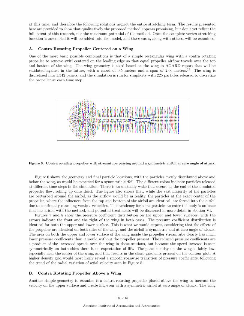
One of the most basic possible combinations is that of a simple rectangular wing with a contra rotating propeller to remove swirl centered on the leading edge so that equal propeller airflow travels over the top and bottom of the wing. The wing geometry is sized based on the wing in AGARD report that will be validated against in the future, with a chord of 0.5 meters and a span of 2.06 meters.29 The wing is discretized into 1,342 panels, and the simulation is run for simplicity with 225 particles released to discretize the propeller at each time step.

A.

Figure 6. Contra rotating propeller with streamtube passing around a symmetric airfoil at zero angle of attack.

Figure 6 shows the geometry and final particle locations, with the particles evenly distributed above and below the wing, as would be expected for a symmetric airfoil. The different colors indicate particles released at different time steps in the simulation. There is an unsteady wake that occurs at the end of the simulated propeller flow, rolling up onto itself. The figure also shows that, while the vast majority of the particles are perturbed around the airfoil, as the airflow would be in reality, the particles at the exact center of the propeller, where the influences from the top and bottom of the airfoil are identical, are forced into the airfoil due to continually canceling vertical velocities. This tendency for some particles to enter the body is an issue that has arisen with the method, and potential treatments will be discussed in more detail in Section VI.

Figures 7 and 8 show the pressure coefficient distribution on the upper and lower surfaces, with the arrows indicate the front and the right of the wing in both cases. The pressure coefficient distribution is identical for both the upper and lower surface. This is what we would expect, considering that the effects of the propeller are identical on both sides of the wing, and the airfoil is symmetric and at zero angle of attack. The area on both the upper and lower surface of the wing inside the propeller streamtube clearly has much lower pressure coefficients than it would without the propeller present. The reduced pressure coefficients are a product of the increased speeds over the wing in those sections, but because the speed increase is seen symmetrically on both sides there is no expectation of lift. The panel density on the wing is fairly low, especially near the center of the wing, and that results in the sharp gradients present on the contour plot. A higher density grid would most likely reveal a smooth spanwise transition of pressure coefficients, following the trend of the radial variation of axial velocity seen in Figure 5.

B. Contra Rotating Propeller Above a Wing

Another simple geometry to examine is a contra rotating propeller placed above the wing to increase the velocity on the upper surface and create lift, even with a symmetric airfoil at zero angle of attack. The wing

10 of 16


−3 −2.5 −2 −1.5 −1 −0.5 0 0.5 1

Pressure coefficient distribution on the top of a wing inside the streamtube of a contra rotating propeller, where the arrows indicate the front and right of the wing.

−3 −2.5 −2 −1.5 −1 −0.5 0 0.5 1

Figure 7.

Figure 8. Pressure coefficient distribution on the bottom of a wing inside the streamtube of a contra rotating propeller, where the arrows indicate the front and right of the wing.

geometry was the same in this case as in the previous one, but the propeller was shifted up by its radius so that the lowest point of the propeller was at the leading edge of the wing. The case was also run with 1,342 panels and 225 particles discretizing the propeller every time step.

Figure 9 shows streamtube contraction as expected, as well as the startup wake from the propeller due to the unsteady nature of the solution. One promising result observed in this figure is the acceleration of particles following the contour of the surface, indicating that the speed increase of the propeller is combining with that of the upper surface of the airfoil. Additionally, we see that the entire streamtube has a slightly negative angle to it, indicating that lift is being produced by the wing.

Figures 10 and 11 show contours of pressure coefficient on the top and bottom of the wing. A slightly lower pressure coefficient value can be seen on the upper surface where the propeller is, compared to the lower surface. The stagnation point in the span section underneath the propeller has been pulled down onto the lower surface, while, if the propeller wasn’t present, the symmetric airfoil would have a stagnation point exactly at the leading edge. This is a result of the fact that the propeller physically pulls air onto the upper surface that, without a propeller, would have traveled over the lower surface instead.

11 of 16


−3 −2.5 −2 −1.5 −1 −0.5 0 0.5 1

Figure 9. Contra rotating propeller with streamtube passing over the top of a symmetric airfoil at zero angle of attack.

Figure 10. Pressure coefficient distribution on the top of a wing underneath the streamtube from a contra rotating propeller, where the arrows indicate the front and right of the wing.

C. Rotating Propeller Above a Wing

The final case examined for this paper is that of a single rotating propeller placed above a wing in the same manner as the previous case. The overall effects due to the propeller velocity should be nearly identical between the two cases, since the particle strengths that cause the contraction and acceleration have been left unchanged. In addition to those contraction effects, this case will no longer be symmetric about the half span because of the rotational effects occurring in the streamtube. This example begins to show the true potential of the method because it can display the asymmetric effects that are common with a single rotating propeller, and account for those same effects in the calculation of force and moment coefficients without the use of a volume grid.

Figure 12 shows streamtube contraction again, as well as the startup wake from the propeller due to the unsteady nature of the solution. A key difference between this case with swirl and the contra rotating case earlier is the appearance that particle density is much higher. This is because, especially farther downstream, the effects of swirl mean that the particles don’t overlap as much, and therefore appear to be more numerous from the side, even though the particle counts are identical for the two cases.

Figures 13 and 14 show contours of pressure coefficient that are similar top and bottom to the case without swirl, with the exception that, with swirl, the distributions are no longer spanwise symmetric. On

12 of 16


−3 −2.5 −2 −1.5 −1 −0.5 0 0.5 1

Pressure coefficient distribution on the bottom of a wing underneath the streamtube from a contra rotating propeller, where the arrows indicate the front and right of the wing. Figure 11.

Figure 12. Rotating propeller mounted with streamtube passing over the top of a symmetric airfoil at zero angle of attack.

top of the wing, the right portion shows that the particles moving away from the wing surface decrease the pressure ever further, while the downward swirling motion on the left portion increase the pressure slightly. On the lower surface there is some slight asymmetry, but it is much less pronounced because the propeller is located on the upper surface. We do see the same movement of the stagnation point onto the lower surface at the span locations near where the propeller is, again indicating that lift is being created even on a symmetric airfoil with no angle of attack, due to the interaction with the propeller.

VI. Ongoing Work

Throughout the course of the work so far, a variety of lessons have been learned that indicate the need for ongoing study of the current method. Once all of the individual components are complete and tested, a final validation will be made to assess the quantitative merits of the overall method. After that, findings with regard to particles entering bodies indicate that research should be done into optimum time step sizes and stepping techniques. Additionally, when, during the research, the three dimensional panel code was selected, it had been written with a steady, single spanwise panel wake, whose overall effect on the quantitative accuracy of the method is currently unknown. Finally, the computational cost of running some of the more

13 of 16


−3 −2.5 −2 −1.5 −1 −0.5 0 0.5 1

Pressure coefficient distribution on the top of a wing underneath a propeller streamtube with swirl, where the arrows indicate the front and right of the wing. Figure 13.

Figure 14. Pressure coefficient distribution on the bottom of a wing underneath a propeller streamtube with swirl, where the arrows indicate the front and right of the wing.

recent cases has also increased, as the desired number of particles and panels has increased, to the point that research into treecode techniques will now be useful.

A. Quantitative Comparison and Validation with AGARD Data

As a final test of the method, once all the individual components have been built and verified, the goal is to compare results from the method with experimental data from AGARD.29–31 The configuration to be tested is a nacelle mounted prop, with the nacelle mounted symmetrically on a wing. The comparison should shed light on the accuracy of pressure coefficient and velocity values calculated on the surface of the model. Panel geometries have already been generated for these tests, so once all verification has been completed the validation can quickly begin. One important prerequisite for the validation is the completion of a model to assign particle strengths in a way accurately reflective of real propellers such as the one used in the AGARD experiment.

B. Time Stepping and Stability

Management of time step sizes throughout the analysis has the potential to vastly alter the run time either positively or negatively. The n body problem necessitates a trade between the time cost of a small step

14 of 16


size and the reduced accuracy and particle-in-body problems of a larger time step size. The particle-inbody issue stems from the fact that particle positions are advanced over finite time intervals, and therefore approach bodies in leaps of position rather than continuously. This is a problem because if a time step is too large a particle may be influenced to take a step that places it inside a body representing a physical object, whereas if the particle had moved in its theoretically continuous motion the opposing influence from the body would have repelled it as its distance from the body decreased. Smaller time step size allows for a better approximation of the theoretically continuous particle motion, but each decrease in time step size requires a corresponding increase in total run time to convect particles the same distance, and achieving a large convected distance is important to make sure that the unsteady wake doesn’t influence results in the area of interest. Additionally, only certain particles will likely have a chance to collide with the body, thereby requiring the reduced time step size, while the rest would have a reduced step size resulting in a slower time without any benefits gained.

One subset of potential work that could go into time step techniques is more in depth analysis of the various higher order time stepping techniques, including all the potentially useful Runge-Kutta schemes, to see which is most effective in terms of stability and ability to model the continuous, theoretical particle paths to avoid entry into bodies.

C. Panel Code Wake Method

The quantitative effects of the current panel code wake method with respect to the particle method are still unknown. The current panel code uses a single spanwise wake panel for each chordwise trailing edge panel to which it attaches. The wake is completely regrown, along with all the panel strengths, for each particle time step, rather than actively growing the wake along with the particle stepping. There are many potential methods for wake implementation, and if the current wake method becomes an issue then other methods will be investigated. The ideal method would most likely be a vortex particle wake, implemented alongside methods such as a treecode to drastically increase the speed of n body problems such as this one, while taking advantage of the vortex method framework that is already implemented. The vortex particle wake would also provide the ability to account for dynamic motion of the body, such as perturbations due to gusts, or flapping effects of a flapping wing aircraft.

D. Computational Efficiency Improvements

Finally, since the particle and panel count continue to increase with the complexity of bodies being model, it is becoming important to examine how to optimize the computational performance. One ma jor source of potential gain is a treecode type data structure that would allow for grouping of many particles far away from the point of interest into one influencing point, thereby drastically reducing the required number of computations. A variety of large scale particle methods and panel codes currently implement similar techniques.

Acknowledgements

This work has been supported by NASA Research Announcement Grant NNX07AO14A under the supervision of technical monitor Craig Nickol.

References 1Hess, J. L. and Smith, A., “Calculation of Non-Lifting Potential Flow About Arbitrary Three-Dimensional Bodies,” Tech.

rep., Douglas Aircraft Company, 1962. 2Williis, D. J., Peraire, J., and White, J. K., “A Combined pFFT-multipole Tree Code, Unsteady Panel Method with

Vortex Particle Wakes,” International Journal for Numerical Methods in Fluids , Vol. 00, 2000, pp. 1–6. 3Willis, D. J., “FastAero - a precorrected FFT - Fast Multipole Tree Steady and Unsteady Potential Flow Solver,” Tech.

rep., Massachusetts Institute of Technology, 2005. 4Willis, D. J., An Unsteady, Accelerated, High Order Panel Method with Vortex Particle Wakes , Ph.D. thesis, Mas

sachusetts Institute of Technology, 2006. 5Voutsinas, S., “Vorrtex Methods In Aeronautics: How to Make Things Work,” International Journal of Computational

Fluid Dynamics , Vol. 20, No. 1, January 2006, pp. 3–18. 6Opoku, D. G. and Nitzsche, F., “Acoustic Validation of a New Code Using Particle Wake Aerodynamics and

Geometrically-Exact Beam Structural Dnyamics,” 29th European Rotorcraft Forum , 2003.

15 of 16


7Opoku, D. G., Triantos, D. G., Nitzsche, F., and Voutsinas, S. G., “Rotorcraft Aerodynamic and Aeroacoustic Modelling Using Vortex Particle Methods,” ICAS Congress , 2002.

8He, C. and Zhao, J., “Modeling Rotor Wake Dynamics with Viscous Vortex Particle Method,” AIAA Journal , Vol. 47, 2009, pp. 902–915.

9Chorin, A., “Numerical study of slightly viscous flow,” Journal of Fluid Mechanics , Vol. 57, 1973, pp. 785–796. 10Winckelmans, G. S., Topics in Vortex Methods for Computation of Three- and Two-Dimensional Incompressible Unsteady

Flows, Doctor of philosophy, California Institute of Technology, Pasadena, California, February 1989. 11Winckelmans, G. and Leonard, A., “Contributions to Vortex Particle Methods for the Computation of Three-Dimensional

Incompressible Unsteady Flows,” Journal of Computational Physics , Vol. 109, 1993, pp. 247–273. 12Rehbach, C., “Numerical Calculation of Three-Dimensional Unsteady Flows with Vortex Sheets,” Aerospace Sciences

Meeting , 1978. 13Chorin, A. J., “Vortex Methods,” Les Houches Summer School of Theoretical Physics , 1993. 14Saffman, P. and Baker, G., “Vortex Interactions,” Annual Review of Fluid Mechanics , Vol. 11, 1979, pp. 95–122. 15Leonard, A., “Vortex Methods for Flow Simulation,” Journal of Computational Physics , Vol. 37, October 1980, pp. 289–

335. 16Beale, J. T. and Ma jda, A., “Vortex Methods I: Convergence in Three Dimensions,” Mathematics of Computation ,

Vol. 39, No. 159, July 1982, pp. 1–27. 17Beale, J. T. and Ma jda, A., “Vortex Method II: Higher Order Accuracy in Two and Three Dimensions,” Mathematics

of Computation , Vol. 39, No. 159, July 1982, pp. 29–52. 18Beale, J. T., “A Convergent 3-D Vortex Method With Grid-Free Stretching,” Mathematics of Computation , Vol. 46, No.

174, April 1986, pp. 401–424. 19Filkovic, D., APAME - Aircraft Panel Method Documentation/Tutorial , July 2009. 20Katz, J. and Plotkin, A., Low-Speed Aerodynamics , Cambridge University Press, 2001. 21Maskew, B., Program VSAERO Theory Document , NASA, contract report 4023 ed., September 1987. 22Benfatto, G., Picco, P., and Pulvirenti, M., “On the Invariant Measures for the Two-Dimensional Euler Flow,” Journal

of Statistical Physics , Vol. 46, No. 3/4, 1987, pp. 729–742. 23Williamson, J., “Low-Storage Runge-Kutta Schemes,” Journal of Computational Physics , Vol. 35, 1980, pp. 48–56. 24Butcher, J. C., The Numerical Analysis of Ordinary Differential Equations: Runge Kutta and General Linear Methods ,

Wiley Interscience, 1987. 25Conway, J. T., “Exact Actuator Disk Solutions For Non-uniform Heavy Loading and Slipstream Contraction,” Journal

of Fluid Mechanics , Vol. 365, 1998, pp. 235–267. 26Conway, J. T., “Prediction of the Performance of Heavily Loaded Propellers with Slipstream Contraction,” Canadian

Aeronautics and Space Journal , Vol. 44, No. 3, September 1998, pp. 169–174. 27Degond, P. and Mas-Gallic, S., “The Weighted Particle Method for Convection-Diffusion Equations Part 1:The Case of

an Isotropic Viscosity,” Mathematics of Computation , Vol. 53, No. 188, October 1989, pp. 485–507. 28Degond, P. and Mas-Gallic, S., “The Weighted Particle Method for Convection-Diffusion Equations Part 2: The

Anisotropic Case,” Mathematics of Computation , Vol. 53, No. 188, October 1989, pp. 509–525. 29Samuelsson, I., “Low Speed Propeller Slipstream Aerodynamic Effects,” Tech. rep., FFA, The Aeronautical Research

Institute of Sweden, 1994. 30Samuelsson, I., “Experimental Investigation of Low Speed Model Propeller Slipstream Aerodynamic Characteristics

Including Flow Field Surveys and Nacelle/Wing Static Pressure Measurements,” Congress of the International Council of the Aeronautical Sciences , Vol. 17, FFA, The Aeronautical Research Institute of Sweden, 1990, pp. 71–84.

31Samuelsson, I., “Low Speed Wind Tunnel Investigation of Propeller Slipstream Aerodynamic Effects on Different Nacelle/Wing Combinations,” Congress of the International Council of the Aeronautical Sciences , Vol. 16, Congress of the International Council of the Aeronautical Sciences, August-September 1988, pp. 1749–1765.

16 of 16


jacob s. calabretta robert a. mcdonald

Documents