j3 of the mean strength, and m is ideally a material
TRANSCRIPT
AN ABSTRACT OF THE THESIS OF
ERNEST YEHEZKEL ROBINSON FOR THE MS IN NUCLEARENGINEERING
DATE THESIS IS PRESENTED April 16, 1965
TITLE: SOME THEORETICAL AND EXPERIMENTAL ASPECTSOF DESIGN WITH BRITTLE MATERIAL
ABSTRACT APPROVEQ Signature redacted for privacy.
The Weibull theory, an attempt to account for the variability of
measured strength in brittle materials, is described in some detail.
An important and useful modification is derived, the normalized sur-
vival probability distribution, given by the equation
S = exp {-m[F(l + l/m)]m} (1)
where S is the probability that the specimen will survive the fraction
j3 of the mean strength, and m is ideally a material constant called
the Weibull modulus. The symbol F denotes the gamma function.
Some of the theoretical implications were investigated in a series
of strength tests made on tubular BeO specimens by pressurizing them
to failure. The results of these experiments were in good agreement
with the theory. The test apparatus developed for this study appears
to offer a useful addition to laboratory methods of measuring the ten-
sile strength of brittle materials.
Equation (1) is a simple analytic expression and can be used to
deduce many aspects of the strength behavior of brittle materials. For
example, the behavior of least values (that is, the strength of the weak-
est specimen in a sample of size n) may be estimated by the formula

for the most probable strength of the weakest specimen. This least
strength 13' is given by
1/rn(m-1 1
mnj F(l+1/m)Since the behavior of the least values constitutes the engineering
limitation to the application of brittle materials, design must be based
on an understanding of least values. The possibilities of influencing
the least values by proof testing to eliminate the weak elements, or by
prestressing (bias), are examined. It appears that the benefits of
proof testing may be limited because mechanical damage may be in-
duced even at low stresses.
It is suggested that the safety margin be given as the extremeM
safety factor, defined as the ratio of the most probable least strength
to the operational stress, which in terms of the requisite failure prob-
ability F is given by
k fm-ix mF
Many of the useful formulas of the Weibull theory are approxi-
mated by simple forms which may serve as practical rules of thumb.
Some general aspects of design philosophy are considered and a
number of design rules are proposed.
For purpose of general information, the variance of the Weibull
distribution and its least values are computed and plotted, demonstra-
ting the superior reliability of the extreme values and the interesting
double-valued nature of standard deviation for certain combinations
of sample size n and Weibull modulus rn. A table of stress
*13= (2)
1/rn(3)

distributions and the corresponding "risks of rupture" is presented and
may be used in circumstances where a complex stress distribution is
to be approximated by more tractable forms.

SOME THEORETICAL AND EXPERIMENTAL ASPECTS
OF DESIGN WITH BRITTLE MATERIAL
by
ERNEST YEHEZKEL ROBINSON
A THESIS
submitted to
OREGON STATE UNIVERSITY
in partial fulfillment of
the requirements for
the degree of
MASTER OF SCIENCE
June 1965

APPROVED:
Signature redacted for privacy.
Typed by
Professor of Mechanical Engineering
In Charge of Major
Signature redacted for privacy.
Head of Department of Mechanical Engineering
Chairman of School Graduate Committee
Signature redacted for privacy.
Dean of Graduate School
Date thesis is presented April 1.6, 1965

TABLE OF CONTENTSPage No.
I. Introduction . . 1
II. Theory . . 2
A. The Weibull Distribution Functions 3
B. The Effect of Size and Stress Distribution 5
The Size Effect 6
The Effect of Stress Distribution 7
C. Finding the Weibull Modulus, m . . 9
D. The Normalized Stress Distribution 12
E. Application of the Normalized Stress Distribution 19
F. Design Considerations 20
Extreme Value Statistics 21
The Proof Stress and Prestress (Bias) 24
Safety Factor 27
System Survival . 31
The Extreme Safety Factor 32
III. Experimental 33
IV. Specimens 37
V. Apparatus and Procedure 43
VI. Results 53
VII. Discussion . . 67
Conclusions . 73
Bibliography . 77
Appendix A: The Risk of Rupture for the Bendingand Bursting of Tubes . . 81

Appendix C:
TABLE OF CONTENTS(Continued)Page No.
Appendix B: Errors Induced by GeometricIrregularities 85
Extreme Value and Mean Value ofthe Truncated, Unbiased WeibullDistribution 89
Variance of the Unbiased, UntruncatedWeibull Distribution and its Least Values 93
Risk of Rupture for Several SimpleStress Distributions 97
List of Tables
Table A. Essential results summarized from Data Tables1-5
Data Table 1. Burst test of one group of round tubes
Data Table 2. Burst test of a second group of round tubes
Data Table 3. Combined burst test data from a third groupof round tubes together with the data fromData Tables 1 and 2
Data Table 4. Modulus of rupture results for BeO tubes
Data Table 5. Results of burst tests of fragments frommodulus-of-rupture tests
List of Figures
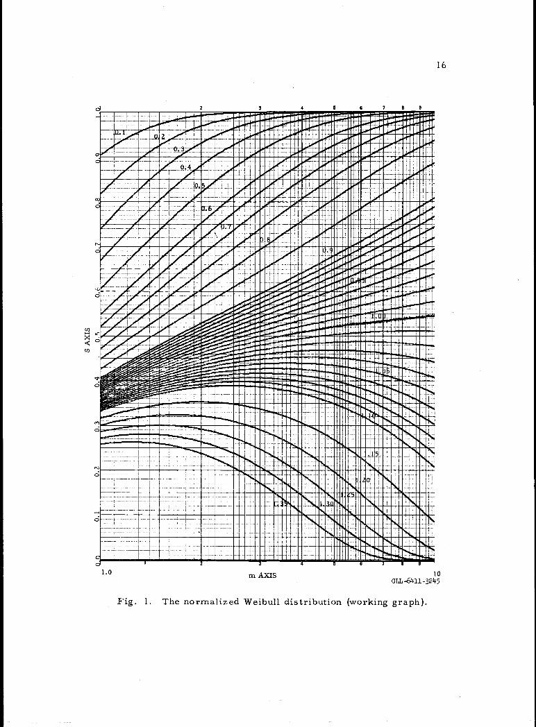
Figure 1. The normalized Weibull distribution(working graph)
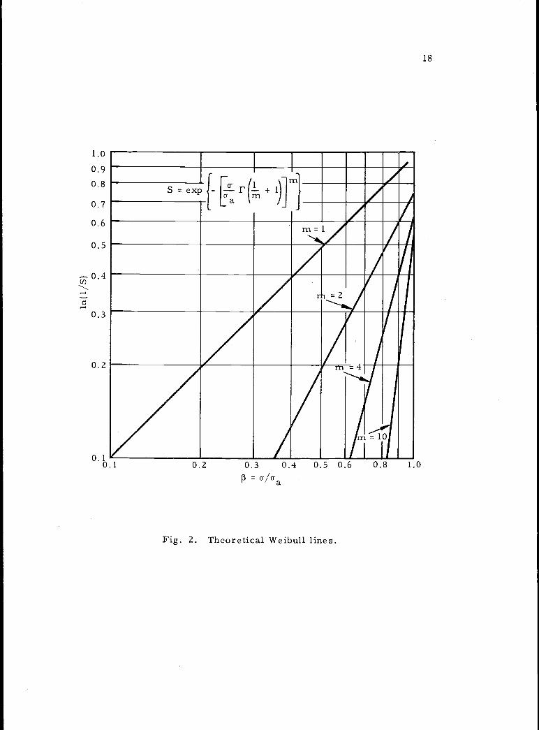
Figure 2. Theoretical Weibull lines
Figure 3. Extreme values (minima) of the reduced Weibulldistribution (normalized)
Figure 4. Theoretical strength improvement due to bias
Figure 5. Material safety factor vs Weibull modulus, m
54
57
59
24
26
30
Appendix D:
Appendix E:
61
63
65
16
18

List of Figures (Continued)
Page N
Figure 24. Standard deviation of various sample sizesas a function of the Weibull modulus . 96

SOME THEORETICAL AND EXPERIMENTAL ASPECTS
OF DESIGN WITH BRITTLE MATERIAL
I. INTRODUCTION
Brittle materials, materials without the capability of plastic
deformation and usually characterized by a compressive strength which
is several times the tensile strength, are more and more frequently
necessary in designs which require a precise knowledge of their
strength behavior. Most refractory materials are brittle, and their
application, for example as fuel elements in gas-cooled reactors or
in hypersonic leading edges and in rocket nozzles, requires a very
high reliability. Even 'ductile" materials under certain biaxial stress
conditions, or at high strain rates, fail in a brittle fashion. The
strength of such materials is, unfortunately a variable quantity and
must be studied statistically. The classical design safety factors
must be redefined in terms of reliability. Effects of size and stress
distribution may be critical and must be understood. In large systems
cracking may indeed be unavoidable.
The evaluation of the requisite statistical parameters for a set of
strength data is expedited by the methods presented here. Aspects of
design reliability are considered in relation to the classical safety fac-
tor and methods of successfully predicting the extreme values, i. e.
the weakest specimens, are established.
The technique of burst-testing of brittle materials developed for
this study and some of the analytical results should prove to be of
value for the investigation of, and design with, brittle materials.

II. THEORY
The most distinguishing feature of experimental strength data on
brittle materials is the wide distribution of the data. Many specimens
are found to be significantly different from the mean, even in very
closely controlled testing. Such a situation leads to a dangerous un-
certainty in designs which are based upon mean values. A design
philosophy based on probabilities of failure and reliability require-
ments has gradually evolved from the foundations of Griffith (12, p. 163-
198) and Weibull (25, no. 151; 26, no. 153). Such an approach is pos-
sible for ductile materials as well, but the relatively small deviations
of strength about the mean value allow a practical design to be based
on the mean value alone.
The premises of the theory of strength of brittle materials, as
advanced by Weibull, establish the importance of tensile stress as the
failure mechanism and the existence of a random distribution of flaws.
The flaws are of random intensity, and fracture, initiated at any flaw,
is assumed to precipitate failure of the specimen. It is evident that
large specimens favor the presence of extreme flaws and hence should
be weaker. The fact that stress concentrations tend to remain high in
brittle materials (in ductile materials plastic strain improves the
stress distribution thereby reducing the stress concentration) implies
a development of the fracture at lower values of nominal stress and
supports the "weakest link" mechanism of brittle failure, which is
fundamental to this theory.
The theory will be reviewed here in sections Il-A, -B, and -C
and certain new modifications and their applications will be described
2

in the remaining sections. The calculations which are specific to the
experimental portion of this study are given in section III.
A. The Weibull Distribution Functions
Consider a material which, at a uniform stress condition, has a
probability of failure per unit volume P0. The probability of survival,
S, of a volume V of the material is given by
S (1 (1)
for the simultaneous survival of V volume units. Taking logs of equa-
tion (1) gives
in S V in (1 - P0). (Z)
Weibull defines the risk of rupture as R-inS and, in terms of an
infinitesimal element, gives
dR = -in (1 - F0) dv.
The term -in (1 - F0) is assumed to be a positive function, n(o),
of the tensile stress o alone. Substitution gives:
dR n(a-) dV
and
R = nfr) dv."V
From the definition of R we get:
exp [cn(o) dv]. (3)
A form for n(o-) suggested by Weibull and justified by its agreement
with experimental results is
n(o-) =1-icrm

4
where and m are constants. This leads to an expression for S in
the following form.
S = exp [- (/)m dvi. (4)
Equation (4) is used in analyzing strength data from brittle ma-
terials and frequently provides satisfactory approximations. It is,
furthermore, sufficiently simple to allow closed form solutions for
many real stress distributions.
In equation (4) the risk of rupture isti m
R=\(---1 dv. (5)
The risk of rupture varies from 0 to as the survival probability,
S, varies from 1 to 0. This implies a variation in a- from 0 to 00; that
is, specimens of 0 and infinite strength exist. It is, of course, evident
that an upper bound must exist, and if such a bound is taken as the
maximum theoretical molecular strength, values are obtained which
are 100 to 1000 times the usual mean values of strength. It is then
reasonable (except for very small volumes) to take the upper limit as
infinite, very small volumes will have mean strengths closer to theo-
retical but subject to great variations (1). Whether or not the lower
strength limit for a material exists may be difficult to determine if it
is near zero since a continuous process of selection exists as speci-
mens are machined and handled. Because of such handling most
specimens will actually exhibit a finite lower bound. If a significantly
high lower bound exists, it will be manifested in the analysis of the
data, and in such cases an added degree of freedom to the proposed

function n(o), in the form of lower bound stress, is required.
This modified form was also proposed by Weibull, as
n(o-) =
- 0I U
n(cT) -I\0 -0-\Swith the provision, of course, that n(cr) 0 when o <o or o > o.
But this form is not at all convenient.
The implications of the theory with regard to the effect of size
and stress distribution can now be examined.
B. The Effect of Size and Stress Distribution
The importance of size is well known in tests of ceramic materi-
als. The size effect, 1. e. , the decrease of strength with increase in
size, and the dependence of strength on the stress distributions are
aspects which i-nay be predicted by this theory, whereas in the past
there was no unified explanation. The prediction of a size effect
m
m
5
and the distribution function becomes
s = exp [S (
-0.u)dVJ
m(6)
and is known as the general Weibull distribution function, This form
of the function greatly complicates the integration for the risk of rup-
ture. However, a rather extensive bit of curve matching can be
achieved with it, since there are now three arbitrary parameters.
Another form, proposed to account for a maximum value of the
variable above which the probability of survival vanishes (26, no. 153),
is

V2.
6
followed by a comparison of expected strengths for the case of uniform
tension and uniform bending will be shown as examples. In the follow-
ing, the form of equation (4) will be assumed.
1. The Size Effect
Consider the risk of rupture for the case of uniform stress
(tension) for two groups of specimens of identical material in which the
volumes subject to such stress are V1 and V2. From equation (5) we
get, using strengths a and and noting that stress is independent of
position,ma
R1 V1,
/R=(-2
If we compare the two types of specimens at the same value of failure
probability or what amounts to the same thing, at equal risks of rup-
ture, then
a1 (V2/ma2 v1)
Equation (8) shows that the strength depends upon specimen vol-
ume and will decrease as the volume increases. Furthermore, the
size effect decreases as the value of m (the Weibull modulus) increases.
Equation (8) is more general than is at first apparent. The risk-of-.
rupture integral, given by equation (5), is expressible in the form
where k may be a normalized geometry integral, and ais
a reference stress. Wherever k does not change between the two speci-
mens the size effect as given by equation (8) will result.
(8)

7
As a numerical example, m will be taken as 10 (a reasonable
value for beryllia). If the volume ratio between two specimens is 10,
then equation (8) gives
-! = 1.26,
hence the large specimens are expected to be only about 80% as strong
as the smaller specimens.
2. The Effect of Stress Distribution
The effect of stress distribution will be analyzed for
uniform bending as compared to uniform tension. In uniform bend-
ing which exists for example between the central loads of a symmetric
four-point loading test, the stress varies linearly through the height of
the beam only:
t
-"1b I-Th£
The volume element for the portion of the span in uniform bending is
dV = b dy.
The risk of rupture for this case is given by substitution in equation (5):m , m
R =(i I (X bdy.B \°oI ocj
Note that integration is carried out only in the region of tensile stress.

Using again the example of m = 10 gives for the expected strength
difference
01D= 1.36,
and the tensile strength should thus be about 7 3.5% of the bending
strength.
These two cases illustrate the marked effect which size and
stress distribution can exert upon expected strength values, and serve
to emphasize the importance of control over the test, coupled with a
proper analysis of the data.
Differences between the results of various stress distributions
observed in practice can now be explained, in many cases with
/B VBRB=-_-) 2(m+ 1)
where VB is the total volume of the beam in the span 1.
The risk of rupture for uniform uniaxial tension in any span is,
as before:m
=() VT.
At the same values of risk of rupture, the ratio of the expected
strengths is given as
- VT 11/rn
(9a)
2 (rn+ 1) (10)
If the volumes are
VB
equal,
1/rn2(m + 1) (lOa)
The result is 8

satisfactory quantitative agreement, on the basis of the Weibull model.
In order to define the statistical strength distribution it is nec-
essary to evaluate the various parameters appearing in equation (4),
of which the most important is m.
C. Finding the Weibull Modulus, m
To evaluate the Weibull modulus from experimental data, equa-
tion (4) is expressed in logarithmic form:
inSS
mdv.
,- \rnIf the integral can be expressed as kV( max where , the
\ °o I maxreference stress, is taken as the maximum fiber stress, then, taking
logs again,
iflifl_rri Dim- 4-S "max"
00
Experimental values of a- and the corresponding values ofmaxsurvival probability may be used to deduce m. A plot of equation (11)
with coordinates in in -- and in a- will produce a straight line ofS max
slope m. If, however, the data does not produce a satisfactory
straight line then the accepted practice is to use a function, n(a-),
modified to include a threshold value as in equation (6), giving
kVininmin(a- -a- )+in.S max U mOO
Using the graphical coordinates in in and in(a- - a- ), onemax u
tries various values of a- until a straight line is obtained. ThisU
9
(12)
corresponds to the general Weibull distribution, given in equation (6),

but only for cases where the risk of rupture is expressible as
/0 - a- \mR=kV(
\ a-c
To this point the exposition is, in general, similar to the various
presentations in the literature. Weibull himself suggests that data
which produce curved lines, when treated as in equation (11), be re-
plotted with various trial values of as in equation (12), until a
straight line is obtained. In general, however, the risk of rupture
does not integrate to the form kV( a-U) It should be noted that
equation (12) evolves from the assumption of equation (6) only if a-u is
assumed to follow the same spatial distribution as a-, although Weibull
treats a- as a constant. The assumption of a- being a constant inU u
space has the consequence that equation (12) applies only to the case of
uniform tension.
The risk of rupture for the generalized Weibull distribution will
now be studied with the purpose of finding m, and to show the incor-
rectness in categorically using the method of equation (12).
The function to be integrated ism- a- \
Rz\( u dV.J\ cr
J
whe r e
a- = threshold,u
scaling factor.
10
Clearly the case of uniform tension in a volume V results inm
a- -a- -R_( T u)V (13)
0
whereT
= tensile stress. Equation (13) leads to the form of equation
(12). The case of uniform bending, e. g.., symmetric four-point load-
ing, gives
BcR
m
m ) dv.
In this case the risk of rupture is assumed to be zero at the
stress o-; hence the integration must be taken over the region where
the stress is equal to or greater than a- , and a- is a constant inde-u u
pendent of position.
The integration gives
V
2ifBifOm
Putting in the limits:m
O -if \/ B u'R=z(V+l) if0 ) (
m+ 1(a- ta-)Bc um+ 1
1-
11
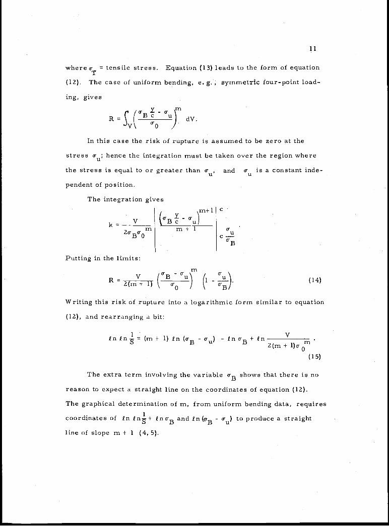
Writing this risk of rupture into a logarithmic form similar to equation
(12), and rearranging a bit:
Vin in (m ± 1) ta-B - -a-B
+ ii2(m + 1)m
(15)
The extra term involving the variable a-B shows that there is no
reason to expect a straight line on the coordinates of equation (12).
The graphical determination of n-i, from uniform bending data, requires1coordinates of £n 1n+ na-B and ln(aB - a-) to produce a straight
line of slope rn + 1 (4, 5).
C
a- uC-a-B
a-u (14)
a-B

The risk of rupture for the case of three-point center loading, in
which the bending is varying linearly in two dimensions, leads to a
nonintegrable form, since
R = 2b
R=
- Zxy -1ma- - a-Bic u dx dy.
a-UIntegrating x first between the limits - - and results in
a-B
C / rn+lScr ia-Ba-m
°B°0 Z(m + 1) u u) yC-a-B
which is not evidently integrable in closed form for general m.
Again it is incorrect to deduce m and a-0 from a requirement
such as equation (12) imposes and data of three-point bending. The use
of WeibuilTs more general distribution function is, therefore, frequent-
ly inconvenient; thus one is led to rationalize, if possible, the use of
the distribution with 0 to approximate more complex distributions.
D. The Normalized Stress Distribution
If attention is confined to the reduced distribution, a- 0, a
certain degree of simplification and insight into the nature of the
parameters is afforded by the use of mean strength, a-, as the normal-
izing factor, suitably substituted fora-0
in the distribution function.
In the following, the equations of Weibull's theory will be re-expressed
in terms of the mean strength, and it will be shown that the failure
probability distribution is explicitly dependent only ona-a
and m,
regardless of the stress distribution or the specimen volume. This
12

or
13
relation allows a straightforward and simple determination of m in
cases where the integration of the applied stress distribution is not
possible, and data of various specimens of a material are at hand.
Equation (4) is assumed to apply and is repeated here for conve-
nience.
The expression for survival probability is equation (4),
exp [-(/)m dv]. (16)
We replace o with f( ) where the reference stress, is taken
as the maximum tensile stress (though it could be any experimental
reference stress), and f() is an appropriate, normalized geometry
function describing the distribution of'stress. This gives
S exp (/)m v [f()]m d}
1 1
mo_f
m
The material and specimen geometry fix the right side of this equation,
and therefore
1 1- in - constant.m Sa-f
If the value of mean strength, °a' is chosen as the reference
stress, to which corresponds the survival probability, Sa then
._L. j! = v ç [f1mdm S m
a- a a-a 0
(17)

and, using equation (18),
exp [ Sa
If we set
x = inS o-a\a
0
rn(in)l/m S0
and, since the integral is F(1/m),
1 E1inS rn rna L
From the recurrence relation
F(1 + x) = xF(x)
mljda-.
0 a
-x 1/rn-ie x dx
(19)
14
which equated with equation (17), gives
s = exp [in Sa(L) (18)
Equation (18) is a simpler and more convenient expression of
equation (4), which may be applied directly to any test result regard-
less of the stress distribution. It replaces the parameter m by the
more familiar 0a (mean strength). The integration is replaced by
n Sa a value obtainable from the data.
in Sa can, however, be given as an explicit function of m only.
The mean value of strength °a' is
a- =1 Sdo-a
then
0 -a

Equation (21) is general for the reduced Weibull distribution and will
prove much more useful than the form of equation (16). For compari-
son, the logarithmic form is
ininmin_+mnr(i+L).°a m
If we use f"a and the corresponding survival probability is
denoted by S, then a combination of equations (20) and (21) yields
a
With equation (21)the Weibull modulus m can be plotted against
survival fraction for various values of 3 . This equation is valid for
any stress distribution, provided the initial premises are met. The
graphs of equation (21) are shown in Fig. 1, where /°a Figure2 is a plot of equation (22). Note again that the foregoing consider-
ations have replaced by the mean value, °a' and eliminated the
integration of the stress distribution.
An analogous approach on the general distribution function having
a bias value, can be employed. It is necessary to assume
that the threshold stress, varies through space in the same way as
the applied stress, so the two bear a constant relation to one another.
This allows the quantity - 0u)m to be factored out of the geometry
15
we get
in.i-a [r(
1mmj (20)
Putting back in equation (18):
mS exp-I i0 1r(l + - (21)
l.0La \ m
N0
0
0
0
0
0
-. ____._--.--pp
:lIP! u..P':.11.P U UI.- - I11p...u..Pll..uu1UuPlII.P,llIup dIUluldpPP
- PlIpIP 119!IP II up0.3 rdm::: dl..puI.II .iulrP -i"r'J& illU aUUP.lIII mlIl II .ilIr .u.Up.UP pi uIpuIPil0.4
L..3
Fig. 1. The normalized Weibull distribution (working graph).
!d I
iII!jiI1Ip!U. 491 .pIdIhi ii. dlP
4F .- Up.-4F !.PAr .4 .4U .p. UP .0IUU fØPll
-UUUUlUU.. Ull
PIIIIIIIUUUU - !uuIiIpu.. !UUi.....-!IIII-; -- urn 11PI1 .UU1uU1IU3'uIplI! UUlII'Uliii 'I!I UUUIIlulu. u iuuiok;11.
'I
10GIL6k1132L5
16
d 4 7 9
1.0 in AXIS

C
C
U,
C
C
Fig. 1. (Continued)
17
3 4 S- --- ____ _._ ---------------------- -
__p USPlU dlUUuIPduII UIIUII_IlUUII.IIIPIIUUUP..lUUIIIIIPi1IIIJ!!idIIIIIUUIlIIuIuIIr..w.i.iiP .uuuiuuu.iiu...iiiii.
lUUlIIIIIUPiIIUUUUuI.u.l...uI.IuIP iiiiiiUUUUIiIiiuiiiii.uui.....IIIi.-- ,:d_p- - .....Psuuiiuiiiuuii... UI ilY r' d eIIIuIluIumuuuuSu uP ..iurnp uiiuu':uuu I
.P'd RiNIIIIiIuiIiiIuuIdUUUUUIiIu.......uuui.uiiuuiUUIIIuiUuiPPlUU!u'_ISIiIIIuIIUIIIU.UUUIIII...... IuIIiIIiIIuI,Iuuuuuuu51
ui.uuuuuuui Iu.uu IU u ...u...uuuiuiiuiii.u. U..II I .i,....ii... U...uliibiiiiiuiuiui.u... 11111!!!!!!U!!!!!!!!!!!!! !!!!!!
1:11,11ill-I
.....uI.i....iiiiiIuIiI--- -
-T _.'!! 11111; ; -i. ..__... . .uuiiiu .u ii. Iuusii.flm.i lu.iu iunui,uuu ui muu IuuuIuIIiiiIuui III IIIIIIIiIIIIuISuuIIINIiIIaiIIuIIuiUiiihiiuIIIIIITuIuIIIIumIII IIIIIIIIUIU UUi IU IIIiiu.i i.Iuui.iIi III IIUUIIIIIiIIU I U UIIII hUN U UiW i.i
I !! E!! 9'f!'!-' IuI
jip I.uihiiI III
u.u. ..s.ium.I'_... UUIIIIUiiuiiuiiiiiiuuiii...uuiui.i.i.'u ....i.u..Ui UUIhUUIU
uu:uuU . IIIiU.. I IllI!I rII.uuInhIIuIh'uIniIII1IUIIUUIIUhIUUhUu. IUIIuUUuIpU..0u1.uui uIIUIPI.. !U1I11.- .uuuuI.._. uuIua.u_..r'- 1.I
I 00GL-611-326
1.10m AXIS
0'C
NC
CC
1.0
0.90.8
0.7
0.6
0.5
0.3
0.2
0.1
I-I
S exp _2:_ r.a
A
AI
Fig. 2. Theoretical Weibull lines.
18
01 0.2 0.3 0.4 05 06 0.8 1.0

integral, as with equation (16), and eventually leads to
r ha -Ii! US exp I(a - r(i
LL\a u) m
E. Application of the Normalized Stress Distribution
The correspondence of the experimentally obtained distribution to
the form of the theoretical distributions of equation (2 1), Fig. 1, or of
equation (22), Fig. 2, or the more complex form of equation (24), will
confirm the theory. The recommended method of evaluating a set of
data is to normalize the experimentally obtained strength values, divid-
ing by the mean strength, and rank them in a monotonic order of size.
The cumulative probabilities are computed by rj/(Ntotai+ 1)
is the rank of the ith entry. These are tabulated and plotted on the
graph of Fig. 1. An uncertainty interval is plotted parallel to the
nearest1
parameter line (see data plots in Results).
The value in the region approaching 3 = 1 must be treated with
caution since theI
lines become nearly horizontal and a small uxtcer-
tainty in probability has associated with it a very wide band of m values.
If the plot resulting on Fig. 1 be approximated by a vertical line,
then the reduced Weibull distribution with a single m value describes
the data.
If the line curves either to the right or left, a complex distribu-
tion is indicated, involving at least two values of m, of the form (for a
duplex distribution)
S = A exp f
m1
i+1 }+(1-A)exP[F(l+rn) mZ)
m}
where r.1
19
(24)

20
or a threshold value is necessary, such as equation (24).
There are several interesting features to the graph of Fig. 1.
It is used, in effect, to make several determinations of m by testing
various portions of the data. If the data is not precisely fitted by a
single value of m, the quantitative errors in estimating failure prob-
ability may be directly evaluated when an approximate m value is
assigned. Such an immediate perspective of the errors of approxima-
tion is not afforded by the plot of Fig. 2, nor is this plot as sensitive
to differences in m.
F. Design Considerations
The fundamental precept of design with brittle materials would
seem to be a definition of an acceptable performance probability.
Thus, the requirement may be, for example, for less than 0.1% prob-
ability of fracture. Such a statement should also be accompanied by
further levels of assurance such as confidence limits and other statis-
tical paraphernalia. On the other hand, due regard must be given to
the concept of nondestructive fracture. This concept refers to condi-
tions of material fracture which do not produce system failure. Such
events occur, for example, with thermal stress fracture of brittle
components which retain their overall geometric stability although they
may be permeated with thermal stress cracks. It is evident that for
nondestructive fractures to exist, such cracking must provide relief
from load. Therefore the loading must be redundant. This element of
nondestructive cracking seems analogous to the plastic deformation
of ductile materials which promotes improved stress distribution and

21
hence provides local relief. The philosophy of design with brittle ma-
terials must recognize the possibility of "crack-tolerant't design while
attempting, as a rule, to prevent fracture. It seems reasonable to
conjecture, therefore, that design with brittle materials will evolve to
more redundant loading configurations so that tensile cracking will not
precipitate failure. Design with ductile material employs the safety
factor or safety margin which is usually applied without regard to
material properties other than mean strength. Weibull's modulus, m,
for metals is usually greater than 40, and the size effect is therefore
very small. Thus, if size is increased to reduce working stress, no
penalty results. It is an entirely different situation with brittle materi-
als where safety factor must be considered in light of the size effect.
Another new concern of design with brittle material is the statistical
behavior of the extremes, i. e. , the weakest specimens in a given
group.
The implications of these considerations will be examined below.
1. Extreme.Value Statistics
When data evaluation must be based on statistical methods because
of a significant variance in some measured parameter, a number of
unique problems present themselves. These result from the necessity
of interpolating or extrapolating test results to provide a forecast of
operational behavior. The first problem is to express quantitatively
the degree of certainty associated with the data and to establish a
satisfactory design philosophy based on this knowledge. The second
problem is the use of a parameter which appropriately describes the

22
central tendency of the data. Third is the problem of extreme values,
their magnitude, distribution, and expectancy. The third problem is
the most crucial aspect of a design which must be based on significantly
variable data, and in which the survival of a system depends entirely
on the statistics of the extreme values, i. e. , those lowest values which
are sufficient to cause failure. In these terms the central tendency
(mean, median, most probable value) is almost irrelevant. A few
aspects of extreme value statistics will be given,to emphasize this kind
of analysis for development of design philosophies with variable phe-
nomena, and particularly where the occurrence of an extreme value is
likely to be a costly or dangerous proposition.
It is required to estimate the magnitude of the extreme (in this
case the lowest extreme) value which may be expected in a sample of
size n. For this we follow the development of Epstein (8, p. 140).
If S(x) is the survival probability at x (cumulative distribution),
the probability that a series of n specimens will contain a value less
than x is
G(x) = 1 - (25)
The differential or frequency distribution, g(x), is found by
differentiating,
g(x) -nsS
where s is . The mode, or most probable value, of the extreme-
value frequency distribution is found by determining its maximum:
n-i 2 n-2g (x) -ris S - n(n- i)s S = 0.

or
s'S = -(n - 1)s2
The value of the variate satisfying this equation will be the mode
of the extreme-value distribution. The normalized Weibull distribution
with = 0 (equation 21) can be used in this formula to find the mode of
its extreme values.
S e1'(1 + 1/m)]m
m-1sS cm3 S,
m-2 r m= cm SIcmI3 - (m - 1)
Putting in equation (26), gives for the mode of extreme values of 3,
* (m it/mr i1) Lru +
A similar form for the case a- >0, with a- /cr = a, can be ob-u u a
tamed, using the assumption at the end of section D and equation (24):/ 1/mrm- 1' 1
p = (1 - a)( ) +a. (27b)U \ mnj Lr(1+1/m)
Using equation (27a) where a- = 0, the graph of the mode of ex-
treme values. for varying sample size and modulus m is given in Fig.
3. Here is seen the very core of the difficulty with brittle materials.
As the number of specimens is increased the extremely low value drops
fairly rapidly, particularly for the lower values of m. Note, for
example, that for m = 6 a sample of 100 specimens will probably
contain one specimen whose strength is only half of the mean. Further-
more this least value is itself a statistical parameter and is distributed
according to equation(25) which may be written as
e113''(1 + 1/m)}m
(27a)
23
(26)

24
::::;I...,.a;;UU ii u,u.iiu I1I U:ik.....0 NIU 11 iji LU uu IIHi. UUIIIUIIIIIIW III IllIllIllI liii III iliiiIlhUUUUUU1IUUUIUIIIII III IHIIIIUIIIIII 11111 II18IlI Hhljlll IIIHi U UUIUIIIIIIIIIH IU.UIHUIIIIII lUll III iuuIilllUUUUUIIUUUllUUllI Ill HHIIIUUUIII Hill IlItPFHi . . I liii Ill liiiU UlIlIillIlIflI IlIflhllUlIl lUll III 111i9,buuUUUUUUUUUIIIIIII Ill flhlflhiillUul Ill Ill Iiii - ..---- II 11111
....UuUU.UpIsuI liIUhIhUuII Ill I III I I .....uuihuiiuuuifl UUIIIUIIIIIIII IN lIHhlJ I.. IIIlIIIth IUUuUUhUUhU IHUUUI U UI I liii I UUUUUUIIHUIIIIIIII IIIIIIIIUUIUIIIII I II Hill I
1.0
:Ilhihihl H I I UUUU.UUU1UIIIUIII IlIllIflhlIll lUll Ill Ill dill HiUUUUUUUNUIUiI IllIllIUhl III 11111 UUUUUUUUUUIIII1IIIII HHIIUUUIIIIIHI I liii 111111 iPU
UUUUUUUUUUUUiI . II I huH I UUUUUUUUIUIIIIIIIIUUIUUIHUUI liii lUll IIIHi.U.UUUUUIUU Ulilil lIIIIIIhIhhIIllHi UUUUiUiUilIIlIIUUIiIhiIIIl 11111 lUll liii lil I... / I I I 11111 llflhlII
UUUUUUUUUUN F ..........- UUUIIUIl!hlIUhllhIIHhUIuIll H hUH U IIUUU 11111 hhlildIlUUUUUUUUUUUI............. iiiil Nll18iII - IHihlllIIhIlllIl 1111111181 IIIllLUU Ill 111111UUiUUUIU........... . I111i18 UUUUUUUUIUIIIIIIUiIUI................UU 11 U U UI I I I III III 11111111,UUUUUUUUUIII ii..iili ii Ullrn....._ UUUUUIUIUIIIIIIIIIIINIUIIIIIIIII IIthUI iLHi - -!........I 11111111 I 111111
HiiiOiHOi I "!!!!Id[di rHb HddIOiM!1IHH1IHIHI ,, :::1uuIIuruq1 IIPHII 'lJIltfljj1
uI1IIw IuuUHhhhIIIII!lflInrip9IuI IU!IEEIIIi!IP Will Jh'hlhi!IIu.JiIui!!JII1lIIllOIIIIiiii llihO:Iilfl .IlI'
UUUUUUUUUUIIII III INUIUIUU UUUUUhII u!UIIUIIIU II IllIIii . .UUUUUUUlU...: IIUUUUUUUUUUIII II USIUIIII HiUUU III UIIIIHUUI HIUIIIU II IUIIIIIIIIJI....UUUUUUUIIIIIIIII I, UIIp11IHHImHIUIIIIIUUUUUUUUIUU1ii II III IIIUUU UUU 1111111 .. IlUhlilluN II h1U UIlIiIUIIUUUU..UUhIIIhhI 11111 hIll. ..? hUIlIIIIhlhhhlIIIII........luiIi II I IflIlk. IIIUUlk ! UUUUUIIIIU. IHNNIII II. I IIIIIIIlUUUUNUUUI. _IUlI III IIIHIUIIUHI ....111111HiUUUUUUUiUUUH II I I IIIUIM 1. IUUU UUU.. UUUIIIIIIIIII lii i.. iii ill hUll.. . IIIIIHiUUUUUUUUIUIiIII.... IIIUUIIIIIIII nhIilIiiIII...
fifi!!9'liIHlW:.::.:I!:l::.:IHnI IuuiuIi!uuIuII!l:IIu.IIwI mi uI:Iflu..!!fluhIIII.ii1...'!uflhlUdh'J bImii!!ii!E'Jj ;;u iiI i!uuuwJIjjuuij'1'1
1111" IIIIIIP N1lO.lUIlImI. hiilhlh" 'Ir1liUUUUUUUU III... HiUh 1111111. I I I I N..ZUU I
UUU r .. II. U .UUqqH hUll
idldbiO!HuII IIIIIIIUII10 20 30 40 50 60 80 100 200 400 600 1000
NO, OF SPECIMENS, n GLL_611-32 7
Fig. 3. Extreme values (minima) of the reduced Weibull distribution(normalized).
2. The Proof Stress and Prestress (Bias)
For purposes of design the existence of a threshold strength may
be of great importance since there is theoretically no failure at stresses
below this level. The possibility of artificially establishing a thresh-
old1 by a bias or a proof test for example1 is of great interest. Further-
more1 the set of specimens containing a threshold should exhibit an
enhanced average strength, provided no internal damage has been sus-
tained, since the weaker specimens in the initial population will be
biased byo or eliminated by the proof stress.
The increase in strength due to a bias on a group of specimens
in uniform bending may be estimated by equating the risks of rupture
with and without a bias, equations (9a) and (14).
1.1
0.8
0.6
0
00.4
0.2
0

25
Using the strength with a zero bias and as the strength with a
bias of a- , where a- is a constant in space:U U
/ a-\mi U\ -micr -cr il--1a-B U, \ °BJ B
If we set s = a- / , the "bias ratio," thenB uB
a-B - (im/m+'1.
(28)
The term a-B/crB may be called the "strength-improvement" ratio.
Thus, if a uniform bending strengtha-B
is desired of a population
exhibiting a strength Th(th a "zero" threshold) and modulus m, the
bias needed is sBcrB where5B
is given in equation (28). If the assump-
tions at the end of section D are imposed on a- the bias ratio will beU
given in all cases bya-BS =- - 1.
The analysis of bias threshold in tension follows analogously and
givesa- -a- a-T u T
whereT
is uniaxial strength with zero threshold anda-T
is the
strength with threshold a--u
To achieve a desired strength °T' the bias required is
0 =O -a-.u T T
Dividing byT as in the previous case and using 5T = a-u/crT gives
a-TS ==--1,
T
Equations (28) and (29) are plotted on Figure 4.
(29)

10.08
6
4
0.4
02
01
TENSION
RENGTHAS
wIT
rIIENGTH WITlAS
H
HOTJ T
I j II1 0 4 6 8 10 20 40 60 80 100
STRENGTH IMPROVEMENT, a-/i GLL-66U-329
Fig. 4. Theoretical strength improvement due to proof testing.
26
The second means of creating a threshold, the screening or
proof test, results in a truncation of the initial distribution. Appendix
C describes some analytical aspects of such a distribution, when it is
initially unbiased. The most probable extreme value is given by a
formula identical with equation (Z7a) provided the truncation 4' is less
than the predicted value p A critical number of specimens can be
deduced from this formula by inserting 4' for For sample sizes
above this number the most likely least value is 4' itself. The mean
value of the truncated distribution relative to the initial (unbiased)
mean value is given by
m m= 4' +e4' F
\e_(ttmd.
No effort was made in the present investigation to study experimentally
the effect of truncation. A graph of vs 4' is shown in Appendix C.
lASa-U

27
It is not expected, however, that all of the improvement suggest-
ed by these equations can be realized. It has been observed that brittle
materials subjected to a stress below the ultimate will exhibit micro-
cracking and slip-band formation and upon subsequent testing will ex-
hibit a reduced strength (19,p. 36-45). An apparent example of this is
observed in the present investigation where the burst strength of frag-
ments from the bending tests is considerably below that of previously
unstressed specimens. This is described in more detail in section VI.
3. Safety Factor
The relationship between reliability and safety factor is given by
equation (21) in which the factor o/o is the inverse of the safety
factor. Now, whereas 0a is essentially invariant with size for metals,
which are characterized by high values of m, as the size of a ceramic
structure is changed to reduce the working stress, the value of o a
must be re-evaluated for the new volume and stress distribution, be-
cause a relatively low value of m implies a significant size and stress
distribution effect, as discussed in section B-i.
Let
= mean strength,
V = volume at which o- is evaluated (from test specimena a
configuration).
As volume is varied the nominal stress will change in accordance
with'V(ao-=o- fi-aV

S expf- 1
kt
F(1 + l/m)1}
28
where f is an appropriate function of volume. The safety factor, how-
ever, must be based on the mean strength of components which have a
volume of V, and the stress distribution.
Referring to equation (8) for the size effect,
01 (V2 1/rn
°Z
The new reference mean strength for components of volume V
is given byV l/m
Now, whereas the classical safety factor is0
c o- f(V/V)
the "truet' safety factor will be given by
(V /V)1/ma
t o- f(V/V)a
or, in terms of the classical factor,
kr/k VJ
and substituting equation (31) into equation (21) we get
(32)
(1 + 1/rn)m}
or
/V a"\VJ

strength by
11=
2(a\vjIf size effect is neglected, the classical safety factor will be
given by2
0 /k a1V
C o a
The size effect, however, specifies that the mean strength of the
component be less than the reference specimen by virtue of its greater
volume, in accordance with equation (30); therefore, the true safety
factor, equation (31), becomes, in terms of the classical safety factor,
k k(1-1/2m)
t C
Z9
The graph of Fig. 5 (reproduced from ref. 17) gives the mate-
rial safety factors for two levels of reliability for various m values.
These values of safety factor must be applied to a mean value which is
corrected for size.
Consider, for example, the case of a rectangular beam in which
the stress is varied by varying the height only. The stress will be re-
lated to volume by
const0
V2
If the mean strength is measured in specimens of volume Va the
stress in the working component of volume V is related to the mean

'-3 t:1 n 0 z Cr)
'-3 z '-3 H H N)
-o
- H
YD
RO
-ST
ON
E P
LA
STE
R
-- M
ILD
ST
EE
L A
T T
EM
PER
AT
UR
E O
F L
IQU
IDA
IR (
FRA
CT
UR
E)
- C
HA
MPI
ON
'S P
OR
CE
LA
II'T
MA
TE
RIA
L S
AFE
TY
FA
CT
OR
DE
NSE
SIL
ICO
N C
AR
BID
E
GR
APH
IC (
BA
RE
)--
MO
LY
BD
EN
UM
DIS
ILIC
IDE
NIC
KE
L-B
ON
DE
D T
ITA
NIU
M C
AR
BID
E
- M
ILD
ST
EE
L (
YIE
LD
STR
EN
GT
H)
GL
ASS
FIB
ER
S
00
00
0
0) 0
4. System Survival
Let us assume a mean strength °a' for a sufficient number of
test specimens of unit volume with a Weibull modulus m. The typical
operational component is B times the size of a test specimen, and n
such components make up a system. An estimate of the survival prob-
ability for the system is required.
First we assume for this example that the size effect is given by
equation (8) (the risk of rupture is kV(0/00)m). The mean strength of
the operational component is, then,
31
(35)
In a group of n such components, the weakest specimen is ex-
pected, by equation (27a), to have a strength of
cr cra\rnnB ) F(1 + 1/rn)(rn-1 1
1/rn
If B is taken as unity, this equation becomes identical with equation
(27) and is described by Fig. 3
The survival probability of the system, as a function of applied
stress, in terms of the component mean strength is
s = exp{n[ F(1 + 1/m)]m}
or, using the test specimen mean strength and the relative component
volume (see equation (32)),
s = exp{-nB[-
F(1 + l/rn}. (36)
or, approximately for low failure probability F,
F Bflm[F(l l/m)}m.

32
5. The Extreme Safety Factor
It has been assumed that failure of the weakest specimen, at
will precipitate system failure. An "extreme safety factor" - as con-
trasted to the classical safety factor of part 3 - can be defined on this
basis as the ratio of the most probable extreme, o, to the operational
stress, a-.
k =
Putting in for its value from equation (35),
O I \1/rnk a(m-1 1
\mnBJ F(1 + 1/rn)
In cia/cr we recognize the classical safety factor, k, sok / 1x 'm-1 /rn
-mnB ) ( 1 + 1/m)
This equation is identical inform with equation (27a) and is described
by the graph of Fig. 3 if the product nB is taken together.
To establish the "extreme safety factor" for a given value of
system reliability we use equation (36)m
in - = nB F(1 + 1/rn)
where S is the desired survival probability. Again, k = °a"°' and
kc = (nB)1/mF(1 + 1/m)(in
Combining with equation (37),
k =(rn l)1/m /(in -x\m s1
(37)
'(38)

33
For the very low probability of failure, F, which must be used in de-
sign the following approximation can be made,
n F.
This gives, approximately, for the "extreme safety factor,"
k Jm 1\1/mxmF)
This equation shows how the true margin of safety decreases
as F increases. As a numerical example we take F = for a
man-rated system and m = 10. The extreme safety factor is, then,
about 6. If the total volume, nB, relative to test specimen volume is,
say, 100, the classical safety factor, from Fig. 3, will be about 9t
This concludes these limited analytical studies. Some of the
theoretical implications were investigated in an experimental study of
the strength behavior of BeO specimens, and are described below.
III. EXPERIMENTAL
In order to study the applicability of the foregoing considerations
to a particular material, a series of tests were carried out using
beryllia (BeQ) specimens in the form of thick-walled tubes, 0.308 in.
o. d., 0.Z30 in. 1. d. , and approximately 5 in. long. These specimens
are described in section IV.
The effect of stress distribution and volume could be studied by
using a standard three-point (center loading) bending test for modulus
of rupture and comparing with strength values obtained by pressurizing
the interior to failure (burst test). The burst-test apparatus which was
developed for this study is unique and appears to be a useful and prac-
tical technique. The apparatus used is described in detail in section V.
(39)

There were three goals to the experimental study:
1. The application of the Weibull statistics to a group of
strength tests, and demonstration of the use of the normalized
expres sions.
Z. The result of pooling several groups of such tests and the
reliability of extreme-value prediction (i. e. , forecasting
the weakest observed values).
3. Prediction of the relative burst and bending strengths.
As the experiment progressed, some of the fragments of the bending
tests were burst-tested. The unusually low values of strength observed
seemed inconsistent with the burst strength of full-length tubes. At
this point a brief study was made to see if microstructural damage
could be induced by moderate stresses, without gross fracture, in the
13e0. The results seemed to be affirmative, and therefore significant
to the aspect of proof testing as a means of improving strength behav-
ior, by creating a prescribed threshold.
The computations for the comparison of burst and bending
strength require the evaluation of the integrals in the non-normalized
Weibull distribution. The details are given in Appendix A, and the
results, using a subscript P to denote pressure
given in the form
34
and B for bending,are
mo_P \ 2
o-OP1/r0
m/ B
I B' 2RB r0 BCB
\ °B /

/ \l/mUp (CB
= 0.665.
35
where r0 is the outside radius and i the stressed span.
The graphs of the constants C and CB are given in Figs. 6 and
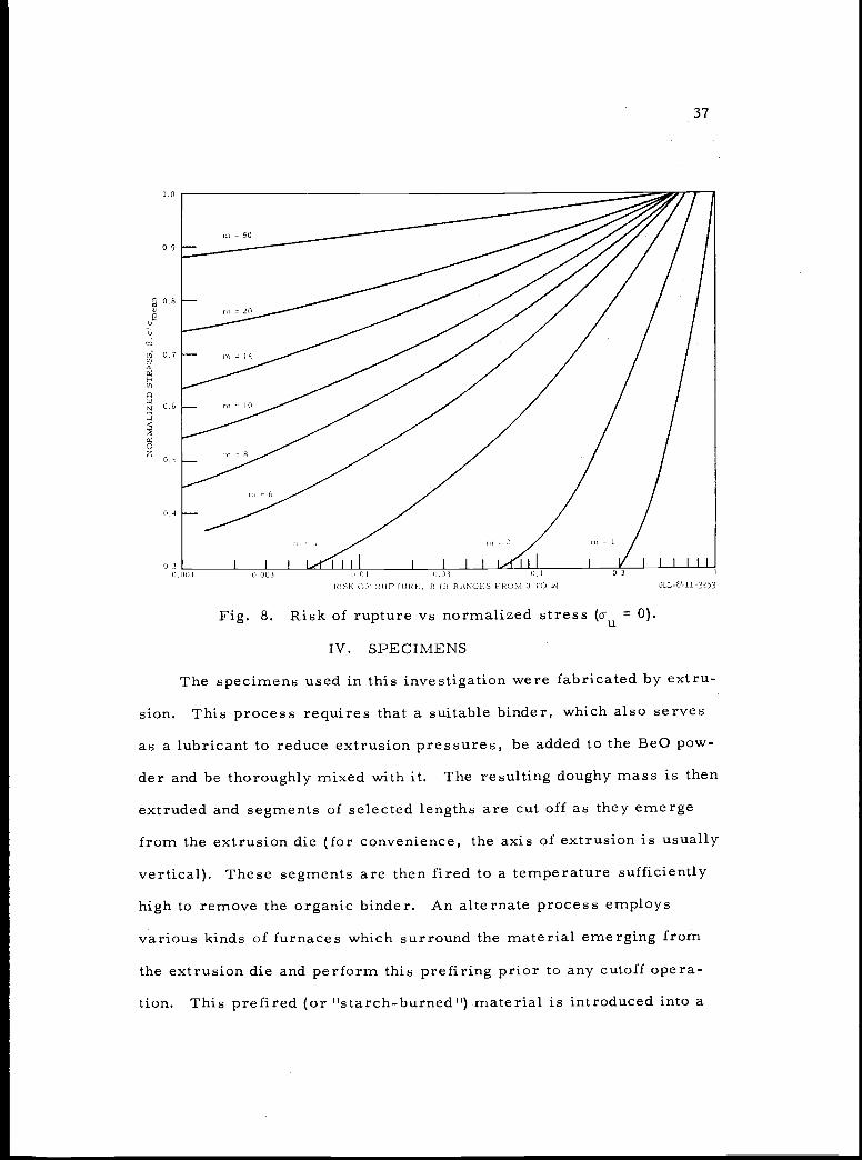
7. If we invoke the relation (see Fig. 8)
R [pI'(l + 1/m)]m (42)
where 3 = 1 at the mean value, and solve equation (40'I and (41) for the
desired strength relation, the following is obtained:
r(i + m ) (r02 BCBo_p_ Up \ p
°B (i+ m) (rl/mp
As an example, assume mB = m = 10; B' e.,
= 0.74;
and take CF and CB from the graphs of Figs. 7 and 8. TheP B
expected strength ratio would be (see Fig. 9):
(43)
We find, therefore, quite a significant difference to be expected
between the burst and bending strengths.
To summarize, then, the m-value is found for each series of
tests by normalizing the data and plotting on Fig. 1. The extreme
value graph is used to check the prediction of the extreme value; and
to compare absolute magnitudes of the bending and burst strength,
equation (43) is used with, if possible, the assumption that=P B

LI
0.8
0.6
0.4
1.0
08
0.6
0.4
0
0
m =ao 4 0 a
36
Fig. 7. Risk-of-rupture coefficient for round tubes under three-point symmetric bending.
= RISK
COEFFICIF001OF
8 1ng1h
RUPTURE K=()m
F
r21
I I
C _____
iiiniiuiP*_1jiIj!iiiIII
pressure.Fig. 6. Risk-of-rupture coefficient for round tubes under internal
r0 OUTER RADIUS R RISK OF RUPTURE
= LENGTH r
C = COEFFICIENT i r0
(
I I
r0Z! CB
CO GLL-6(0J.i 325
b-a
CB GLL-611 -3252
37
R[SK 0 U RU P 1URF, R (U RANGES F ROM 0 TO GLL-6511-3253
Fig. 8. Risk of rupture vs normalized stress °u = 0).
IV. SPECIMENS
The specimens used in this investigation were fabricated by extru-
sion. This process requires that a suitable binder, which also serves
as a lubricant to reduce extrusion pressures, be added to the BeO pow-
der and be thoroughly mixed with it. The resulting doughy mass is then
extruded and segments of selected lengths are cut off as they emerge
from the extrusion die (for convenience, the axis of extrusion is usually
vertical). These segments are then fired to a temperature sufficiently
high to remove the organic hinder. An alternate process employs
various kinds of furnaces which surround the material emerging from
the extrusion die and perform this prefiring prior to any cutoff opera-
tion. This prefired (or "starch-burned") material is introduced into a
38
high temperature kiln where it is fired for several hours at temperatures
approaching 1700°C. This is the sintering process and the parts emerge
in a hard, densified condition. Let it be noted that this kind of manu-
facturing technique is still very much an art and apparently minor
manipulations at various steps may produce profound changes. This is
particularly true at the mixing stage.
In order to produce the tubular shape a mandrel is used which is
supported "upstream" of the die by a "spider." The spiders used had
either three or six legs. The flow gradients around these legs and the
specific shape of the die inlet will influence the final fired geometry.
The tubular specimens had an inside diameter of about 0.230 in. and
outside diameter of 0.308 in. A number of test specimens were mea-
sured very precisely for concentricity and roundness on an Indi-Ron
machine to examine wall thickness variations and ellipticity. The
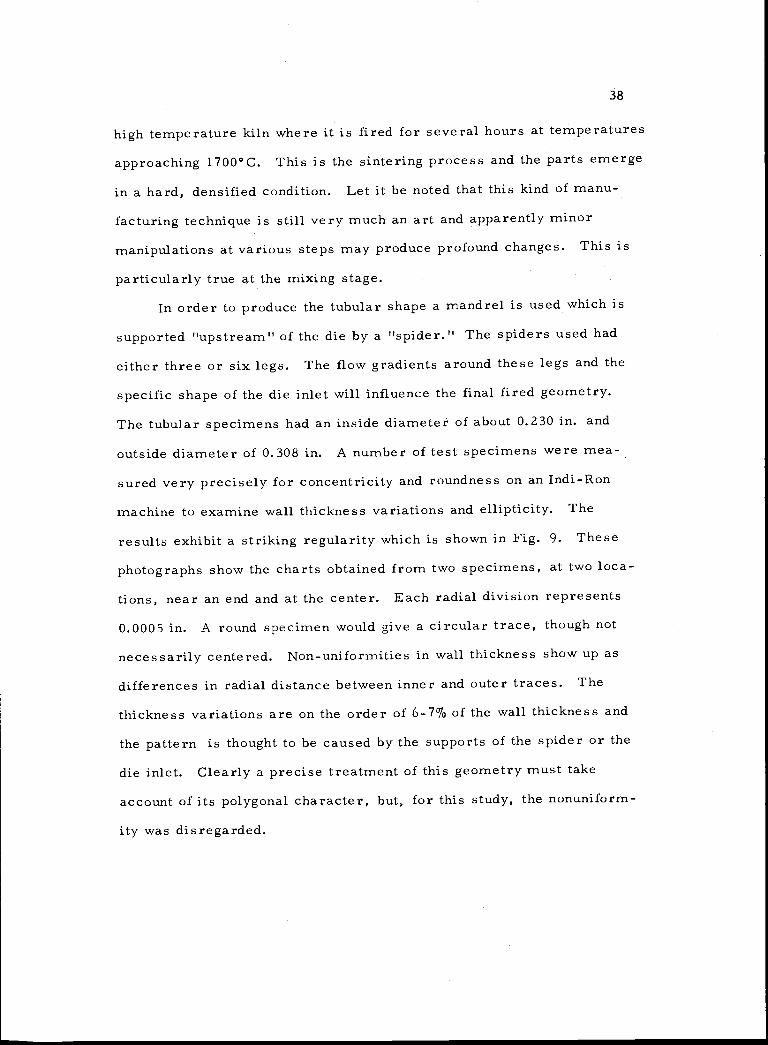
results exhibit a striking regularity which is shown in Fig. 9. These
photographs show the charts obtained from two specimens, at two loca-
tions, near an end and at the center. Each radial division represents
0.0005 in. A round specimen would give a circular trace, though not
necessarily centered. Non-uniformities in wall thickness show up as
differences in radial distance between inner and outer traces. The
thickness variations are on the order of 6-7% of the wall thickness and
the pattern is thought to be caused by the supports of the spider or the
die inlet. Clearly a precise treatment of this geometry must take
account of its polygonal character, but, for this study, the nonuniform-
ity was disregarded.
I NDI-RON
()
7 INDI-RONhOt)<1OIVISlON
Fig. 9. Roundness charts of test specimens.
-65 _1171
39

40
Another important factor in contributing variability is the grain
size distribution which varied in a regular way from the interior to ex-
terior surfaces as shown in Fig. 10. It would be unreasonable to assign
a single value to grain size and yet grain size is a well-known influence
in the strength of materials (15). This introduces still another element
of uncertainty into the present study.
The mechanical aspect of proof testing which is described in
section II (Theory) was examined briefly because of the disparity ob-
served between the strengths of fragments from the bending tests (data
table 5, section VI) and specimens which were previously untested (data
tables 1, 2, 3). The method used was to grind a flat about 1/8 in. wide,
axially on a specimen and then to polish and etch it (using hydrofluosili-
cic acid at 90°C). After taking photographs of this "unperturbed"
surface (Fig. 10 a, b) the specimen was loaded in bending to various
increasing stress levels and re-examined after each stress cycle until
evidence of damage was observed, as shown in Fig. 11. These photo-
micrographs show one of the specimens after loading to a nominal stress
of about 35 ksi, at the polished surface. Cracked and broken grains are
visible. This early breakup may indicate the advent of structural
damage at stresses below the ultimate and that a proof test as a means
of raising or creating a lower threshold must be approached with wari-
ness. Figure lOc, at Z000X, shows what seems to be a microcrack
about 0.0005 in. long. At the present it is not certain that these features
were definitely caused by the stress cycle.
The observed strength anisotropy between bending and bursting
(which exceeded the predicted difference) may be the manifestation of

IB-b4ll-7G2U
z000x
Fig. 10. Grain size variation in test specimen.
a) b) 41
500X 500XNEAR INSIDE BORE NEAR OUTER SURFACE
(c)

l000x
42
100 ox
Fig. 11. Microstructural damage due to proof stress. Direction ofstress is along axis.
AXIS
AXIS
EDGE OF- FLAT

43
an observed microstructural anisotropy. The BeO powder used in
this fabrication was of the UOX grade supplied commercially by the
Brush Beryllium Corporation. This particular material is derived
from beryllium sulfate and characteristically contaLns many needle-
shaped particles (laths) which, during the extrusion process, are
oriented parallel to the axis of extrusion. Subsequently, during the
sintering cycle grain growth occurs about these laths producing a pre-
ferred orientation in the final grain structure.
Prior to testing all specimens were inspected by fluorescent
penetrant in order to eliminate any which contained visible cracks.
V. APPARATUS AND PROCEDURE
Two kinds of tests were run on the BeO tubes: a standard three-
point bending (center loading) test, and a unique burst test for which
a special apparatus was devised. The major requirement of the
burst test apparatus was to provide means of pressurizing the
interior of a tubular specimen and measuring the pressure atfailure. This must be accomplished in a reproducible fashion so
that the only significant source of variability will be the strength of the
specimen.
The overall apparatus consists of a source of pressurized fluid,
gages, valves and controls, furnace or heater for elevated temperature
work, and the specimen holder. All but the specimen holder are fairly
straightforward components. The specimen holder required some
development.

44
There are, of course, a number of ways to pressurize the inte-
rior of a tube, and the judgment for selecting a particular method re-
quired the following criteria to be met:
The performance of each run must not be fraught with com-
plexity nor demand a meticulous and precise test procedure
to give reproducible results.
The time to perform an individual run must be relatively
short: on the order of a few minutes for room temperature
testing and perhaps four or five times this for high tempera-
ture tests.
The apparatus must be adaptable to testing at various tem-
perature levels.
The apparatus should be of inherently flexible design, allow-
ing the use of various size specimens, and it should be suit-
able for standardized parts.
The specimen holder and apparatus which finally evolved for
this investigation passed through a number of distinct phases. There
were four basic designs tried, which are illustrated in Fig. 12. The
first (Fig. 12a) employed a surgical rubber tube within the test speci-
men and sealed at the ends with special barbs. This method required
a long setup time and was frequently hampered by leaks at the collar
or the actual extrusion of the rubber tube around the collar. The
second design (Fig. lZb) used a Stat-O-Seal, a commercial sealing
device, at the end faces of the tubular specimen. Sealing was accom-
plished by imposing a sufficiently large axial force and, on occasion,
these forces became undesirably large. The third design (Fig. lZc)

a)
SEALING BLOCKSARE BOLTED TOGETHER
SEALING ANTI-EXTRUSIONBLOCK, COLLAR
// * SPECIMEN
RUBBER
'SM4NOBLO K
ENDBLOCK
b)
CONSTRUCTION OFSTAT-O-SEAL" STAT-O-SEAL
SPECIMEN
RUBBER0-RING SEAL
SPECIMEN
RUBBER 0-RING
d) .- - -n MOVEABLE PROBE
STATIONARY SLEEVE
45
NOTE: It was diffi-cult to prevent ex-trusions around thecollar, and in addi-tion, the collar causedleaks. Long set-uptime -
NOTE: High end-loads were requiredto achieve a seal.
METAL WASHERMOLDED-INRUBBER SEAL
Fig. IZ. Sealing techniques tried in the burst test.
NOTE: The tolerancein the specimen borecaused a variation inthe sealing load.
NOTE: Most repro-ducible sealing load.
GLL -6312 -3216A
46
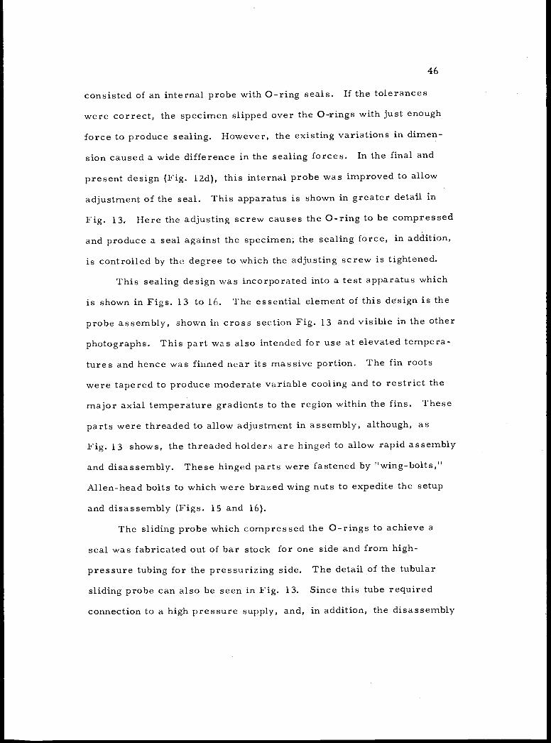
consisted of an internal probe with 0-ring seals. If the tolerances
were correct, the specimen slipped over the 0-rings with just enough
force to produce sealing. However, the existing variations in dimen-
sion caused a wide difference in the sealing forces. In the final and
present design (Fig. lZd), this internal probe was improved to allow
adjustment of the seal. This apparatus is shown in greater detail in
Fig. 13. Here the adjusting screw causes the 0-ring to be compressed
and produce a seal against the specimen; the sealing force, in addition,
is controlled by the degree to which the adjusting screw is tightened.
This sealing design was incorporated into a test apparatus which
is shown in Figs. 13 to 16. The essential element of this design is the
probe assembly, shown in cross section Fig. 13 and visible in the other
photographs. This part was also intended for use at elevated tempera-
tures and hence was finned near its massive portion. The fin roots
were tapered to produce moderate variable cooling and to restrict the
major axial temperature gradients to the region within the fins. These
parts were threaded to allow adjustment in assembly, although, as
Fig. 13 shows, the threaded holders are hinged to allow rapid assembly
and disassembly. These hinged parts were fastened by "wingbolts,"
Allen-head bolts to which were brazed wing nuts to expedite the setup
and disassembly (Figs. 15 and 16).
The sliding probe which compressed the 0-rings to achieve a
seal was fabricated out of bar stock for one side and from high-
pres sure tubing for the pressurizing side. The detail of the tubular
sliding probe can also be seen in Fig. 13. Since this tube required
connection to a high pressure supply, and, in addition, the disassembly

9
I1
I
COOLINGFINS
0 RING SEAL
KEY
TRUARC RETAINING RINGADJUSTABLECOLLAR
THREADS
SLIDING PROBE MADE OF TUBING
MINIATURE COUPLING
'0" RING SEAL
CROSS SECTION THROUGH COUPLINGGLL -6312 -3217A
Fig. 13. Cross section of pressurizing probe.
Fig. 14. The probes and 0-rings.
47

Fig. 15. Burst apparatus - assembly nearly complete.
Fig. 16. Burst apparatus showing induction coils and susceptor.
48

49
requirements imposed a size restriction, a miniature high-pressure
coupling was devised and successfully used for this connection. This
coupling, a simple sliding 0-ring assembly, was pinned by a key
which, when the coupling was pressurized, became locked and pre-
vented accidental disassembly (see Fig. 13).
In order to perform high temperature tests, a suitable sealing
material was needed. The requisite properties were corrosion
resistance and softness. Although such tests are not within
the scope of the present study it is worthwhile to mention some en-
couraging results. It was found that gold 0-rings worked very well in
the temperature region 1300 to 1900°F and nickel 0-rings from 2200 to
2450°F. The procedure was to raise the temperatures above 1200°F
and gradually tighten the adjustment, to cause the metal to flow and
seal the annular gap between the specimen and the probe. Approxi-
mately 30 minutes was required from start to complete disassembly at
the highest temperature. This time interval is satisfactory. The high
temperatures were achieved by the induction heating of a susceptor
which surrounded the test specimen. Various steels and superalloys
were tried but the best results were obtained with a very thick-walled
silicon carbide susceptor, with which temperatures of 3000°F could be
reached in less than 30 minutes. The susceptor also served as a
blast shield during specimen failure. Again, in order to expedite the
test procedures, the induction coil was wound in two transverse sec-
tions and a hinge was devised which allowed one side to be raised
(see Fig. 16). This coil, though adequate to about 1850°F, was too

50
inefficient to achieve the higher temperatures in reasonable times, so
another full spiral coil with varying pitch was used for tempera-
ture in excess of this limit. The apparatus as it appears ready for an
elevated temperature run is shown in Fig. 17.
This final design is shown partially disassembled and assembled
in Figs. 14, 15, and 16. Figure 15 shows the position of the specimen.
with the 0-ring probes inserted, as it would be set up for a room tem-
perature test. The blast shield, which is seen surrounding the speci-
men in Fig. 16, restricts the violent scattering of fragments and, for
elevated temperature testing, serves as a susceptor for the induction
coils. The blast shield is centered by ceramic end caps. The assem-
bled view (Fig. 16) shows the blast shield and caps in place but the
upper coil not lowered for an elevated temperature run. Close-ups of
the specimen holding the seal probes in Fig. 14 show the distension
of the 0-ring (B) when the sliding member (A) is tightened against the
fixed tube (C).
Because of the toxicity of BeO the test apparatus was enclosed in
a ventilated glove box. Figure 18 shows this box in an overall view of
the test apparatus. A1 and A2 are the high pressure supplies of argon
gas and hydraulic fluid respectively. The gas bottle A1, is a Lawrence
Radiation Laboratory (LRL) unit, made and filled at LRL. A2 is a
commercial pneumatically operated high pressure pump capable of
delivering 20,000 psi. The control valves are at B and the gages at C.
The apparatus is inside the ventilated box, D. The induction power
supply, E, is controlled by a Leeds and Northrup Controller, F, and
the three specimen thermocouples are recorded by two pens at G and
one at F.

Fig. 17. Burst apparatus ready for elevated temperature test.
Fig. 18. Overall view of test area and equipment.
51

The instrumentation used in room temperature tests consisted
only of pressure gages. Two Heise pressure gages were used to rnea-
sure pressure in two ranges (15,000 psi full scale and 50,000 psi full
scale). The gages were calibrated every two weeks to 1/4%and ex-
hibited no significant changes during the period of the test work. In
order to measure the pressure difference between the gages and the
specimens, a transducer was connected in place of a specimen and the
maximum pressure difference found to be about 50 psi at 5000 psi.
For the elevated temperature runs to 2400 °F three Chromel-
Alumel thermocouples were placed in contact with the specimen, at
either end and the center as seen in Fig. 17. Any one of the thermo-
couples could be used as the reference by the L & N controller which
controlled the induction power supply. The outputs of all three were
recorded continuously, one on the L & N controller and the other two on
a Honeywell Electronik- 17 two-pen recorder. Temperature gradients
rarely exceeded 2%. Figure 20 gives a schematic of the fluid pres-
surizing and controlling circuit.
FLUIDIN
FLUID OUT
TO APPARATUS
50,000 psi GAGE,
Fig. 19. Schematic of fluid pressurizing and controlling circuit.
52

VI. RESULTS
The experimental results are summarized in Table A and given
in full in the Data Tables 1 to 5. The data is presented in the order
observed and is also ranked in size order, to facilitate normalization
and computation of probabilities. Data Tables 1 and 2 represent two
groups of specimens, which were tested in burst, several months
apart. A third group was tested still later and all three were pooled
to give Data Table 3. Data Table 4 gives the results of modulus-of-
rupture (M-R) tests in symmetric three-point bending. Some of the
fragments from these tests were subsequently burst tested and the
results are shown in Data Table 5. With each of the tables is a work-
ing graph similar to Fig. 1 and a plot of the data and approximate
theoretical distribution.
It is possible that an unusually high failure probability at the
mean value is a manifestation of a relatively near upper bound. The
portion of the distribution which is of prime importance in design,
however, is the region below the mean, where for the burst-test-
results the approximations are quite satisfactory. The M-R data
contain structure and imply a complex probability density, for which
the single Weibull distribution is only a rough approximation. The
formula of equation (44) was still used to compare the theoretically
expected difference in mean strength with the observed value, as shown
in the last entry of the results table (Table A).
53

TA
BL
E A
.E
ssen
tial r
esul
ts o
f st
reng
th te
sts
on B
eO a
t roo
m te
mpe
ratu
re.
Dat
aN
o. o
fM
ean
Obs
erve
dta
ble
spec
imen
sst
reng
th,
extr
eme
rn-v
alue
f3'
no.
ksi
130
21.0
815
.64
9.5
0.73
237
21.8
114
.28
9.5
0.7
310
620
.112
.27
0.55
438
42.1
32.4
9.5
0.7
529
15.8
1.7
30.
32
Pred
icte
d ex
trem
e
The
rat
io o
f bu
rst t
o be
nd s
tren
gth
is p
redi
cted
to b
e 0.
64, o
bser
ved
to b
e0.
48.
Stre
s s
,T
ype
ofks
ite
stR
emar
ks
15.4
Bur
st,
If th
e m
ean
and
4.5-
in,
rn-v
alue
of
Tab
lele
ngth
1 ar
e us
ed to
15.3
Bur
st,
pred
ict f
or T
able
3, th
e ex
trem
e4.
5-in
.va
lue
is 1
3.3k
sile
ngth
11.1
Bur
st,
Pool
ed d
ata
4.5-
in.
leng
th29
.5B
end,
Rou
gh f
it3-
in.
span
5.1
Bur
stR
ough
fit,
no
of M
-R m
ode.
frag
-m
ents

55
The difference is sufficiently large that causes for real strength
anisotropy should be looked for, and indeed they appear to lie in the
nonisotropic grain orientation.
It should, in principle, be possible to pool the normalized results
of the bend and burst tests, but, because of the rough fit to the bending
data, this was not done. The three separate groups of burst data were
pooled in Data Table 3 and seem to be well approximated by the Weibull
distribution, although a slightly lower m results.
Insofar as proof testing is concerned, the microstructural damage
which was apparently induced by stresses below the ultimate (see Fig.
lOc and 11), implies that the benefits of proof testing are likely to be
mixed or even nonexistent.
The extreme value predicted from the Weibull modulus is, in
every case, in satisfactory agreement with the observed extreme
value. This prediction would be used when projecting to large popu-
lations and it is therefore a notable success that predictions for
the 106 specimens of Data Table 3, based on the results of Data
Table 1, are in reasonable agreement.
This method of extreme value prediction was also applied to other
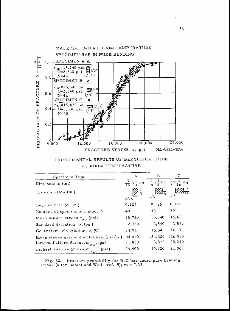
published data, Fig. 20, taken from Daniel and Weil (5). They give
m = 7.25 for 140 BeO specimens tested in four-point bending. The
least value observed was 8870 psi. The value predicted by the graph of
Fig. 3 leads to a value of 8400 psi.
1z
HC-)
0.40
H
o
1.0
0.8
0.2
8,000 12,000 16,000 20 000 24 000
MATERIAL BeO AT ROOM TEMPERATURESPECIMEN BAR IN PURE BENDING
FRACTURE STRESS, a-, psi GLL-64-11-325
EXPERIMENTAL RESULTS OF BERYLLIUM OXIDEAT ROOM TEMPERATURE
56
Fig. 20. Fracture probability for BeO bar under pure bendingstress (after Daniel and Weil, ref. 5); m = 7.25
- - L.a
04a-m'5740 P
0=2,320 psiN48
SPECIMEN B
fl11L/J
/
3/16'o
aa-m'5'54° psi
0=2,540 psiN=42
SPECIMEN C
/' /i/4H
TmiS,6SO pSi0=2,530N=50
3/16'i/' ALAyAtA v
ft.£
:
I0000
A
Specimen Type A B C
Dimensions (in.) >< X4 !)4X4r _XThX4
Cross section (in.)3/16 1/4 1/3
Gage volume (cu in.) 0.125 0.125 0.125
Number of specimens tested, N 48 42 50
Mean failure stress,a- , (psi) 15,740 15,540 15,650
Standard deviation, a, (psi) 2,320 2,540 2,530
Coefficient of variation, v, (%) 14.74 16.34 16.17
Mean stress gradient at failure, (psi/in.) 94,440 124,320 166,930Lowest Failure Stress, a- , (psilow
11,830 8,870 10,210
Highest Failure Stresscrhigh (psi) 19,900 19,320 21,000

Me anburst Mean
pressure strength6200 21.08
57
DATA TABLE 1. Burst tesi of one group of round tubes, i. d. = 0.230in, , o. d. = 0.310 in., = 0.74, o/P = 3.4, stressed length = 4.5 in.
Runno.
Burstpressure,
psi
Burstpressure,
psi
Max.stress,
ksi
Norm.stress
Cumulativefailure
probability probability
Cumulativesurvival
1 6200 4600 15.64 0.743 0.0 32 0.9682 5600 5000 17.0 0.808 0.064 0.9363 6000 5200 17.68 0.840 0.0 97 0.90 34 6500 5300 18.04 0.857 0.129 0.8715 5200 5500 18.7 0.888 0.161 0.8 39
6 5600 5600 19.04 0.9047 6900 5600 19.04 0.9048 6600 5600 19.04 0.904 0.2 50 0.7429 6500 5700 19.38 0.92 1 0.290 0.710
10 5500 5900 20.06 0.953 0.322 0.678
11 6400 6000 20.4 0.969 0.355 0.64512 5300 6100 20.74 0.985 0.387 0.61313 6500 6200 21.08 1.00 0.4 19 0.58 114 7000 6300 21.42 1.02 0.452 0.54815 6900 6400 21.76 1.03
16 6800 6400 2 1.7 b 1 .0 - 0.516 0.48417 6900 6500 22.10 1.0518 6700 6500 22.10 1.0519 5000 6500 22.10 1.0520 4600 6500 22.10 1,05 0.645 0.355
21 5600 6600 22.44 1.0722 5900 6600 22.44 1.07 0.709 0.29123 6300 6700 22.78 1.08 0.742 0.25824 5100 6800 23,12 1.10 0.7 74 0.22625 6100 6900 23.46 1.11
26 6900 6900 23.46 1.1127 6500 6900 23.46 Lii28 7400 6900 23.46 1.11 0.90 3 0.09729 6400 7000 23.80 1.13 0.935 0.0 6530 6600 7400 25.16 1.19 0.968 0.0 32
Observed data Ordered data

01
0
U)
010.
2
0 6
U
3 0,6
0.65
5 0. 750.9
0.8
05
0.4
03
1.0
6
7 8 9 10 20
WEIBULL MODULUS, n30 40 60 100
GLL-6J)11.3255
0
H 0.2I
S.
0.1
0.0
z0
0.3U)
010.
1.1
01
0.40
1..
7.5
7.6
0 0.2 0.4 0.6 0.8 1.0 1.2 1.4
= /MEAN GLL-611-3256Working graph and failure probability plot corresponding to Data
Table 1.
58
004
-4
0.6
0,4
0
-4
0.400.4
- 0.6
-4
0.8
1.0
SS
mU 95
H 0.8-4

59
DATA TABLE 2. Burst test of a second group of round tubes, i. d.= 0.230 in. , o. d. = 0.310 in., = 0.74, a-/P 3.4, stressed length= 4.5 in.
Observed data Ordered dataRunno.
Burstpressure,
psi
Burstpressure,
psi
Max.stress,ksi
Norm. Cumulative Cumulativestress failure - survival
probability probability1 6000 4200 14.28 0.655 0.026 0.9742 6000 5100 17.34 0.795 0.053 0.9473 6500 5200 17.68 0.811 0.079 0.9214 6600 5400 18.36 0.842 0.105 0.8955 6600 5600 19.04 0.873 0.132 0.8686 6700 5700 19.38 0.889 0.158 0.8427 5400 6000 20.40 0.9358 6500 6000 20.40 0.9359 6400 6000 20.40 0.935 0.236 0.764
10 7200 6200 21.08 0.96711 6400 6200 21.08 0.967 0.289 0.71112 6300 6300 21.42 0.98213 6300 6300 21.42 0.98214 6600 6300 21.42 0.98215 6200 6300 21.42 0.982 0.395 0.60516 7100 6400 21.76 0.99817 6300 6400 21.76 0.998 0.447 0.55318 5100 6500 22.10 1.01319 6600 6500 22.10 1.013 0.500 0.520 6000 6600 22.44 1.02921 7000 6600 22.44 1.02922 5200. 6600 22.44 1.02923 7000 6600 22.44 1.02924 4200 6600 22.44 1.029 0.631 0.46925 6300 6700 22.78 1.04426 6700 6700 22.78 1.04427 6200 6700 22.78 1.044 0.710 0.29028 7300 6800 23.12 1.060 0.737 0.26329 7400 6900 23.46 1.076 0.763 0.23330 6700 7000 23.80 1.09131 6800 7000 23.80 1.091 0.816 0.18432 5700 7100 24.14 1.107 0.842 0.15833 6600 7200 24.48 1.122 0.868 0.13234 7400 7300 24.82 1.138 0.895 0.10535 7600 7400 25.16 1.15436 5600 7400 25.16 1.154 0.947 0.05337 6900 7600 25.84 1.185 0.973 0.027
Av pressure 6416 psiAv strength = 21.81 ksi

5 0.65
0 0,7
O 0.75
O 0,8
1.0
0,9
0,
0.6
0.5
1.0
H 0.8
c.0
0.4
10
I II
05
3 4 5 6 7 8 9 10
WEII3ULL MODULUS,
1 MEAN)
I I I I I I I 0720 30 40 60 100
GLL-6.11 3251
S
SIS
IS
II
S
rn = 9.5
0 0.2 0.4 0.6 0.8 1.0 1.2 1.4
= /MEAN GIL-611-3258
Working graph and failure probability plot corresponding to DataTable 2.
60
0. I
0.2
0.6

61
DATA TABLE 3. Combined burst test data from a third group ofround tubes together with the data from Data Tables 1 p.nd 2, i. d.= 0.230 in., o. d. 0.310 in.,
.= 0.74, a-/P = 3.4. Combined data of
106 specimens.
Av maximum stress = 20.1 ksi
Burstpress.
Norm.value
BurstSurv. Norm. Surv.pres.prob. ps1 value prob.Burst Norm. Surv.press. value prob.
3600 5700 65003600 0.608 0.981 5700 65004000 0.675 0.971 5700 0.962 0.616 65004200 5800 0.979 0.607 65004200 5900 6500
4200 5900 6500 1.098 0.2714200 5900 66004200 0.709 0.925 5900 0.996 0.570 66004400 0.743 0.915 6000 66004600 6000 66004600 6000 66004600 0.776 0.887 6000 66004700 0.793 0.878 6000 1.013 0.523 6600 1.112 0.2064800 6100 67004800 0.810 0.859 6100 1.030 0.505 6700
4900 6200 67004900 0.827 0.841 6200 6700 1.130 0.1685000 6200 68005000 6200 6800 1.145 0.1505000 0.844 0.813 6200 69005100 0.861 0.803 6200 69005200 6200 69005200 6200 1.047 0.430 69005200 0.878 0.775 6300 6900 1.163 0.1035300 6300 70005300 0.895 0.757 6300 70005400 6300 7000 1.180 0.0755400 0.912 0.734 6300 71005500 6300 1.063 0.374 72005500 0.928 0.719 6400 73005600 6400 74005600 6400 74005600 6400 7400 1.249 0.025600 6400 1.080 0.328 7600 1.283 0.0095600560056005600 0.945 0.644
Av burst pressure 5924 psi

1.0
0.9
0.8
0F. 0,70
0.4
0.3
B = 0.9
(0
0
1.05
0.2 0.4 0.6 0.8P = /MEAN
""..1F S1(MEAN)
1.01
1.0 1.2 14GLL -6ku -3260
0.5
0.6
I I I I I I I I 0,720 30 40 60 10
GLL-6611.3259
Working graph and failure probability plot corresponding to DataTable 3.
1.0
0.8
6 7 8 9 10
WEIDULL MODULUS, rr
0
H 0.2-I
0. 0.40 0
on0.4 0.6
0.2 0.8
01.0
I I
.S
S
I
7
= 9.5/
62
0
0.1
0.2
B = 0.6
0 0.65
O = 0.7
0 0.75
0 0.8
S = 0.85

63
DATA TABLE 4. Modulus of rupture results for BeO tubes, three-point loading, 3-in. span, ,j 0.74, a-/F 00. Room temperature.Runno.
Maxlgd
Maxstressksi
Ordered stress Normalizeddata stress
Survivalprobability
1 98.4 492 32.4 0.769 0.9732 64.9 32.4 33.2 0.788 0.9473 90.4 45.2 33.5 0.796 0.9224 79.0 39.5 33.7 0.800 0.8965 70.2 35.1 34.2 0.812 0.870
6 89.7 44.9 35,1 0.834 0.8457 91.9 48.0 35.5 0.843 0.8198 84.0 47.0 36.5 0.867 0.7949 95.7 47.8 37.8 0.898 0.768
10 85.1 42.6 39.5 0.938 0.742
11 67.0 33.5 40.7 0.967 0.71712 82.1 41.1 41.1 0.97 6 0.69113 91.4 45.7 41.2 0.978 0.66514 101.3 50.7 4.5 0.986 0.61415 87.6 43.8 41.6 0.988 0.58916 87.0 43.5 42.0 0.997 0.56317 87.5 43.7 42.6 1.012 0.53818 96.7 48.3 42.9 1.019 0.51219 92.2 46.1 43.0 1.021 0.48620 92.5 46.2 43.0 1.021 0.48621 91.4 45.7 43,4 1.031 0.46122 86.8 43.4 43.5 1.033 0.43523 82.4 41.2 43.7 1.038 0.41024 66.4 33.2 43.8 1.040 0.38425 86.0 43.0 44.7 1.062 0.35826 95.2 47.6 44.9 1.06627 73.0 36.5 45.228 75.6 37.0 45.729 83.3 41.6 45.730 89.4 44.7 46.0 1.09 0.205
31 81.5 40.7 46.132 83.0 41.5 46.233 86.0 43.0 47.234 98.5 47.2 47.635 85.8 42.9 47.8 1.135 0.10236 67.5 33.7 48.337 68.4 34.2 49.2 1.16938 71.0 35.5 50.7 1.204 0.098
Av load Av max stress84.2 lb 42.1 ksi

1.0
0.9
0.8
0.4
0.3 I liii I 111110.7
64
1.0
.3 3 4 5 6 7 8 9 10
WEIISULL MODULUS, m30 30 40 60 100
GLL-6411- 261
H-4 02 S
--4
0.60 0
0.4 n-i = 9.5
04 04(COMPLEX)
0.4 0.6
-4 S
02 0.8 .S
Cl) S
1.0
0.2 0.4 0.6 0.8 1.0 1.2 1.4
= /MEAN GLL-611-3262
Working graph and failure probability plot corresponding to DataTable 4.

65
DATA TABLE 5. Results of burst tests of fragments from modulus-of-rupture tests,
.= 0.74, cr/P = 3.4. Room temperature.
Mean pressure 4630 psiMean strength 15.7 ksi
Observed data Ordered dataN Burst
O pressure,psi
Burstpressure
psi
Normalizedvalue
Survivalprobability
1 5500 5002 3900 500 0.108 0.9323 3600 2200 0.473 0.9004 3600 2400 0.516 0.8675 3300 2750 0.591 0.8336 2750 3300 0.709 0.8007 6000 36008 500 3600 0.774 0.7339 6200 3900 0.838 0.700
10 6000 4200 0.903 0.66711 4200 4400 0.946 0.63212 5800 4600 0.989 0.60013 6200 500014 6200 5000 1.075 0.53315 5000 5200 1.118 0.50016 5200 5400 1.16 0.46617 500 550018 6200 5500 1.182 0.40019 6000 580020 5800 5800 1.247 0.33321 6200 600022 5000 600023 5500 6000 1.291 0.23324 2200 620025 2400 620026 5400 620027 4400 620028 4600 620029 6200 6200 1.333 0.034

1.0
L 7 8 9 10
WEJI9ULL MODULUS m
MAY CONTAIN A THRESHOLD
x./
/0.
NO MODE
I I I
02 0.4 0.6 0.8 1.0 1.2
= /MEANWorking graph and failure probability plot corresponding to Data
Table 5.
66
60 105GLL-601].- 263
1.4 1.6
GLL _61i1 -3261+
c. 0.40 0
0.4 - 0.6m
0.2 0.8
01.0
I
H 0.8 H

VII. DISCUSSION
The present study was concerned with certain analytical modifi-
cations and experimental checks on the statistical strength distribution
of brittle materials. Unfortunately, the literature dealing with
strength studies of such materials frequently fails to give a table of all
results, and the published graphs are difficult to interpret with any
precision. Very often, also, an adequate characterization of the speci-
mens, the material, and fabrication is lacking, and in some cases
conclusions are drawn on the basis of extremely meager data (22, p.
298-300). Since there are many parameters that may contribute to the
variability of strength - grain size, density, fabrication, and test
technique, to mention a few - it seems appropriate here to specify the
type of information that should accompany strength tests on brittle
material. Identification of the variability due to each of these factors
will contribute to more efficient engineering applications of ceramics
and other brittle materials. It is therefore recommended that strength
studies on brittle materials (or ductile material below the transition
temperature) contain the following information:
A. Starting mate rial description
1. Ceramics
Source of powder
Extraction and preparation of powder
Relevant properties of the powder
Quantitative analysis of constituents
2. Non-ceramics
a. Source
67

68
Initial preparation and fabrication history
Quantitative analysis of constituents
B. Fabrication
Ceramics
Powder preparation
Binder addition
Pressing or extrusion conditions
Firing sequence
Final test specimen fabrication and geometry
Grain size as well as size and spatial distribution
and the method of measurement
Density
2. Non-ceramics
Final fabrication procedures
Heat treatment (anneals, etc.)
Final test specimen machining and position in
stock billet
Grain size as well as size and spatial distribution
and measurement method
C. Testing
Loading method in detail
Load measurement in detail
Specimen selection
Detailed procedure
D. Results

69
All the raw data in the order observed, or at least the
following: the mean, the number of specimens, and
the extremes.
The data ordered monotonically in magnitude of the
variable
The appropriate statistical parameters describing the
data, and the method of analysis
Although many of these requirements are obvious, there is prob-
ably not a single paper (including this one) which contains all of the
above. The preoccupation with the starting material and fabrication
may serve to elucidate the variability which is frequently observed be-
tween specimens of different batches or lots of the "same" material.
The importance of grain size and density can be appreciated from their
effect on elastic properties and strength (14, p.. 452-453; 15, p. 376-
387). The problem is therefore further complicated by the general
lack of meaningful grain size measurement techniques particularly as
regards grain size distribution. The problem of porosity, that is
density, measurement must ultimately contend with pore size and
shape. The investigation of these "fine structure" effects, however,
must await the elimination of gross causes of variability such as the
geometric nonuniformity of the BeO tubes in this study, and the proper
treatment of the starting material and experimental procedure.
The strength distribution suggested by Weibull seems to fit the
data observed by many investigators (25, 26, 27) and the normalized
form described here provides a quick and useful test for the reduced
Weibul distribution (a- = 0). This simplified form is directly useful in

70
consideration of extreme value statistics and the formula for the mode
of extreme values. The results of burst testing of BeO specimens seem
to be satisfactorily approximated by this theory.
Theoretically some improvement in the mean and extreme value
can be achieved by a threshold, e.g. , as shown in Figs.4 and 23. The
necessary truncation is, however, relatively high and experience seems
to show that proof testing may cause a decrease in strength, which is
evidently due to microscopic damage induced in the proof test (section
Iv, p. 41). The choice of proof testing to create a threshold must
follow careful evaluation.
The section on design reliability gives a link between the
"classical" safety factor and a new and physically more significant
quantity, the "extreme" safety factor (equations (37) and (39)). This,
with the formulas for the mode of extreme values, equations (27),
should prove very usable for design estimates with brittle materials
when a suitable value of the Weibull modulus m is selected. Applica-
tion of the extreme-value formula to the experimental data (Table of
Results) as well as to published data in the literature confirmed its
usefulness. This extreme (least) value has uncertainty attached to it.
Its distribution is, however, known from equation (25). Since the
distributions are known, it is a straightforward matter to compute
standard deviations; however, it is felt that a better measure of dis-
persion is given by the least value. Nevertheless, the standard devia-
tion of the unbiased, untruncated Weibull distribution and its least
values are given in Appendix D. Computations of risk of rupture at
various stress distribution may be facilitated by the formulas in Appen-
dix E.

71
Before the experimental data are discussed the difficulties
associated with testing brittle material (Appendix B) need to be empha-
sized. The problems of the standard tensile test are of course well
known and extensive attempts to eliminate eccentricity in the specimen
and load train have not met with much success. Various other schemes
in the literature (2, 7) have suffered from the complexity of specimens,
and finally, the work of Sedlacek and Halden (22, p. 298-300) on the
burst testing of thin-wall rings seemed to promise a new era of
precision in brittle material testing (coefficients of variation 2%).
Unfortunately, this precision rests on very few specimens (four in one
group and eight in a second, of alumina), and attempts to repeat the
tests at IITRI and at LRL have produced the usual range of about ±10%
of the mean. This is easy to understand when the implications of
slight amounts of ellipticity and nonuniformity (Appendix B) are
considered. The same criticisms, that is of inherent variability be-
cause of geometric irregularities, apply as well to the burst test
performed here on the relatively thick-walled long tubes.
The experimental results of this study generally confirm the
application of Weibull statistics. The extreme value forecast is very
satisfactory, giving agreement which is frequently within a few per-
cent of the observed value. The data of burst testing for two groups of
specimens (drawn from the same lot but tested several months apart)
yielded similar rn-values but differed from that observed for a combi-
nation of these two test series with a third group of similar size; how-
ever the extreme value was predictable with satisfactory accuracy.

72
The distribution of bend strength data is complex an4 the rn-value
chosen is only a fair approximation. It may be that the bend data have
a lower bound, but in any case the bend strength is greater than the
theoretical prediction by an apparently significant margin. This theo-
retical prediction is obtained with equation (44), and the assumption
which it contains may not apply. This "true" anisotropy may be due
in part to grain orientation caused by the lathlike particles in the pow-
der which oriented during extrusion, but there may be other mecha-
nisms as well causing the irregular bend-strength distribution. The
fragments of the M-R tests which were burst-tested gave very erratic
results and a separate, short investigation indicated that prestres sing
may cause microscopic damage. This prestres sing study was based on
a similar one done on alumina at IITRI (19). Such a result is of major
significance if proof testing, as a method of improving strength be-
havior, is contemplated. A careful study of this point should precede
the adoption of proof stress.
The burst-test apparatus and method developed embody a number
of notable features. The specimen is subjected to a tensile stress
over a large majority of the volume (although the condition is one of
biaxial stress and nonuniform tension), and the specimen is of a simple
geometry. In addition the apparatus is capable of burst test at elevated
temperatures, and incorporates several features to minimize the testtime. It provides a new method for "tensile" testing of brittle mate-
rials, in which deviation from the nominal stress distribution is due
almost entirely to specimen geometry and can therefore be controlled
to some extent by careful fabrication and selection. This test is easy

73
to perform and requires little skill. It should be useful, in conjunction
with standard bend testing, for the study of and design with brittle
materials.
CONCLUSIONS
The experimental investigation of the strength of BeO tubes
confirmed several aspects of the Weibull distribution.
The observed strength distribution was well approximated by a
theoretical distribution containing no bias or truncation. The Weibull
modulus for BeO was found to range between about 7 and 10, the lower
value corresponding to other published results (5). The strength dis-
tribution of BeO using the lower value is given by
S e625P7.Essentially the same value of m was obtained for several samples
tested over a time interval of several months, and it is concluded that
there are no significant time-dependent effects on m occurring at
room temperature. The effects of stress distribution and volume under
tensile stress were qualitatively confirmed by the bending data. The
bending strength, however, was higher than predicted, and its distribu-
tion was not as well approximated by the theoretical curve. This was
attributed to grain orientation which resulted from extrusion and mate-
rial effects. The normalized plot (Fig. 1) for data analysis and
approximation was found to be very convenient. The normalized form
of the distribution function is very useful since the mean value and in
explicitly define the distribution function.

74
The observed extreme values were predicted with satisfactory
precision by the theoretical expression
1/mc fm - 1
mn ) F(1+l/rn)and its graph in Fig. 3. This gives further assurance to the application
of the Weibull theory and is of most interest in problems of design
where information on least-value behavior is mandatory.
It is felt that the burst test technique should be of interest in the
study of brittle strength behavior. The test at room temperature was
found to be simple and quick, and although elevated temperature tests
are more difficult they are possible using suitable seals (metal 0-
rings). But whatever strength measurement is used, care must be
taken to consider the quantitative effects of eccentricity as discussed
for example in Appendix B, and, in cases where proof testing is con-
templated, the problems of low-stress damage.
Respecting design with brittle materials, a number of reasonable
design rules may be proposed:
Experiment and material must be carefully characterized.
Data should be approximated by the unbiased, untruncated
function if at all possible. The approximation to least values
is more important than to values near the mean since, as
shown in Appendix D, the least values are statistically more
reliable.
The extreme value and its range should be defined by a
formula of the form of equation (27a).

75
4. The degree of conservatism used in design can be expressed
by the "extreme safety factor" defined by equations (37) and
(39).
5. Attempts to influence the distribution by screening or bias can
be estimated by the analysis of truncation (Appendix C) or the
idealized bias as in equation (24).
6. Several rough estimates can be made using approximations to
various equations as "rules of thumb"; for example:
The value of m can be guessed at using the least observed
value and Fig. 3.
The failure probability at a stress 3 in a sample of n is
guessed at byrnFn3
The extreme safety factor is given approximately by
kx F1/m.
If a sample contains bias, the rn-value can be estimated
from the survival probability at the mean value.
7. As a design principle, it is sometimes desirable to give up
information on stress distribution and magnitude in order to
obtain the benefits of redundant supports as discussed in
Section II -F.
8. Although data is only approximated by the Weibull distribution,
the theory can lead to statistically rigorous design formulation
and is therefore vastly superior to design based on mean
strength and a large factor of ignorance.

76
A number of extensions of this study suggest themselves. The
problems of proof testing, particularly when proof stress and opera-
tional stress have different distributions, should be studied. The
effects of time and temperature on m are of interest, and finally, the
application of this distribution to other phenomena such as stress
rupture and fatigue (as Weibull has done) may prove of practical value.

BIBLIOGRAPHY
Anthony, F. M. and A. L. Minstretta. Leading edge design with
brittle materials. Aerospace Engineering 20:20-1, 44-52.
Nov. 1961.
Barnett, R. L. Review of structural design techniques for
brittle components under static loads. Chicago, 1963. 123 p.
(Illinois Institute of Technology. Armour Research Foundation
vol. 2, AD-4l0262, ARF report no. 8259, Final Report Feb. -
May 1963)
Bodine, E. G. Design with rate-sensitive ceramics. Aerospace
Engineering 22:100-107. Jan. 1963.
Bortz, S. A. and N. A. Weil. Studies on the predictive value of
statistical theories for the fracture of brittle materials. Chicago,
1962. 33 p. (Illinois Institute of Technology. Armour Research
Foundation ASD-TR- 61- 628, Air Force Contract AF33(6 16)-
7465)
Daniel, I. M. and N. A. Weil. Influence of stress gradient
upon fracture of brittle materials. ASME Paper 63-WA-228;
presented at Winter Annual Meeting, American Society of
Mechanical Engineers, Philadelphia, Nov. 17-22, 1963.
Duckworth, W. H. and Alfred Rudnick. The strength of ceramic
materials. Battelle Technical Review 10:3-8. April 1961.
Durelli, A. J., S. Morse and V. J. Parks. The theta specimen
for determining tensile strength of brittle materials. Materials
Research and Standards 2:114-117. 1962.
77

78
Epstein, B. Statistical aspects of fracture problems. Journal
of Applied Physics 19:140. 1948.
Fisher, J. C. and J. H. Hollomon. Statistical theory of frac-
ture. Metals Technology 14:1-16. Aug. 1947. (American
Institute of Mining and Metallurgical Engineers. Technical
Publication no. 2218)
Frankel, J. P. Relative strengths of Portland cement mortar in
bending under various loading conditions. Journal of the
American Concrete Institute 20:21-32. 1948.
11, Goode, H. P. and J. H. K. Kao. Sampling procedures and
tables for life and reliability testing based on the Weibull distri-
bution (mean life criteria). Ithaca, Sept. 30, 1961. 58 p.
(Cornell University. Sibley School of Mechanical Engineering.
Quality Control and Reliability Technical Report TR-3, Office of
Assistant Secretary of Defense, Installations and Logistics)
Griffith, A. A. The phenomena of rupture and flow in solids.
Philosophical Transactions of the Royal Society of London, ser. A,
221:163-198. 1920.
Gumbel, E. J. Statistical theory of extreme values and some
practical applications. Washington, 1943. 51 p. (U. S. Depart-
ment of Commerce, National Bureau of Standards, Applied
Mathematics Series 33)
Hasselman, D. P. H. On the porosity dependence of the elastic
moduli of polycrystalline refractory materials. Journal of the
American Ceramic Society 45:452-453. 1962.

79
i3 Knudsen, F. P. Dependence of mechanical strength of brittle
polycrystalline specimens on porosity and grain size. Journal
of the American Ceramic Society 42:376-387. 1959.
Manson, S. S. and R. W. Smith. Theory of thermal shock
resistance of brittle materials based on WeibuiP s statistical
theory of strength. Journal of the American Ceramic Society
38:18-27. 1955.
McDonough, N. T. Structural reliability of components using
brittle materials. Dallas, Oct. 1961. 41 p. (Chance Vought
Aircraft, Dallas, Texas. Strength analysis report AST/EIR-
13431)
Midgley, E. and F. T. Peirce. Tensile tests for cotton yarns,
theorems on strength of long and composite specimens. Journal
of the Textile Institute 17:T305-T 368. 1926.
Parikh, N. M. Studies of the brittle behavior of ceramic mate-
rials. June 1964. (Wright-Patterson Air Force Base, Air
Force Systems Command, report no. ASD-TR-61-628 Part III.
Office of Technical Services, U. S. Department of Commerce)
Pears, C. D. and S. Oglesby. Evaluation of tensile data for
brittle materials obtained with gas bearing concentricity. May
1963. (Wright-Patterson Air Force Base, Air Force Systems
Command, report no. ASD-TDR-63-245. Office of Technical
Services, U. S. Department of Commerce)
Roark, R. J. Formulas for stress and strain. 2d ed. New York,
McGraw-Hill, 1954. 381 p.
80
Sedlacek, H. and F. A. Halden. Method for tensile testing of
brittle materials. Review of Scientific Instruments 33:298-300.
1962.
Stokes, R. J. and C. H. Li. Dislocations and the strength of
polycrystalline ceramics. 1962. 42 p. (U. S. Government
Research Reports 37:54. HR-62-262 or AD 275-273)
Tippett, L. H. C. On the extreme individuals and the range of
samples taken from a normal population. Biornetrika 17:364-
387. 1925.
Weibull, Waloddi. A statistical theory of the strength of mate-
rials (in English). Ingeniors Vetenskaps Akadamien-Handlingar,
Stockholm, no. 151. p. 1-45. 1939.
. The phenomen of rupture in solids.
Ingeniors Vetenskaps Akadamien-Handlingar, Stockholm, no.
153. p. 1-55. 1939.
. A statistical distribution function of wide
applicability. Journal of Applied Mechanics 18:293-297. 1951.

APPENDIX A
THE RISK OF RUPTURE FOR THE BENDING AND
BURSTING OF TUBES
I. The Three-point Bending of Round Tubes
The risk of rupture will be found from the superposition of two
solutions for the round rod.
Consider the cross section:
R0 =
Using .L = sin 0r0
2 2 2x +y r0 withaxisz
dV=
The stress in terms of the maximum outer fiber stress is
V Z-Br I
where I is the half-span. The risk of rupture for this rod is
/o \m r0 m /R = (-fl \
S0 S0 () Jr - dydz.o)
Integrating the z term,
/ '2 2(B\m 41 /\0) m + I S r) yr0 - y dy.
R 41ii/2 . m - sin29ldO.
0 o) m + r0 5 sin 0(1
81

We have from integral tables
çir/z
0
and
m+2sin OdO=
Cir/2
sin ed r(+i)Putting in, we get, finally:
The difference of the two gives
(mm( iRB \m+] m+2tube \0/ \ /
m+1sin cos 9 m + I mm+2 +m+2 jsin OdO
(1T/2m + Im + 2
VR is the volume of a solid rod of radius0
re-expressed in the form
RB o / 0 Btube \0/
sin edO
rn\ 4Q 2/ m+Im+IrO
r(mJ_VR [Ir(i+i)J
Figure 7 gives GB as a function of ., the radius ratio
82
r (m + F\v/ (A-I)
To find the risk of rupture for the tube the calculation is repeated for
the case of a rod having a radius r.., the inner radius of the tube, and
for which the maximum fiber stress is B = where is thei 0
maximum outer fiber stress given in equation (A_i):m rn (m+I
B'\ (r.\ 4 2( m+]\\ 20) jm+Iim+2)2r+ (A-2)
m+21
(A-3)
(A -4)
r0. Equation (A- 3) may be
rr/2
0

pressure is2r.
10 = p -a-r
II. The Round Tube with Internal Pressure
The tangential stress distribution in thick-wall tubes with internal
( 2r0 + r)
r.1Using--a and!,r0 i r0
(I +0 = p
j2- (i
The maximum stress, at ., is
I +0 max
1
which gives for the variable stress, in terms of a max
/(i '\ (i+max
The differential volume in the annulus is
dV = 2ir dr
where I is the total span under pressure.
The risk of rupture is
Leta =0-.max p
/0- (R= +
cii 0-
R =\ maxp 0O
m7 i 7i+2\I 2r02Id.
I]
m
s' (+!)
83
(A-5)

The integral in equation (A-5) must be integrated by numerical
methods. An IBM 650 computer code was written to perform this
computation. The results were used to expreSs the risk of rupture in
the form
Rp
The constant Cp
in Fig. 6.
r 2 c0 p
in equation (.A-6 ) is plotted against thickness ratio,
84
(A-6)
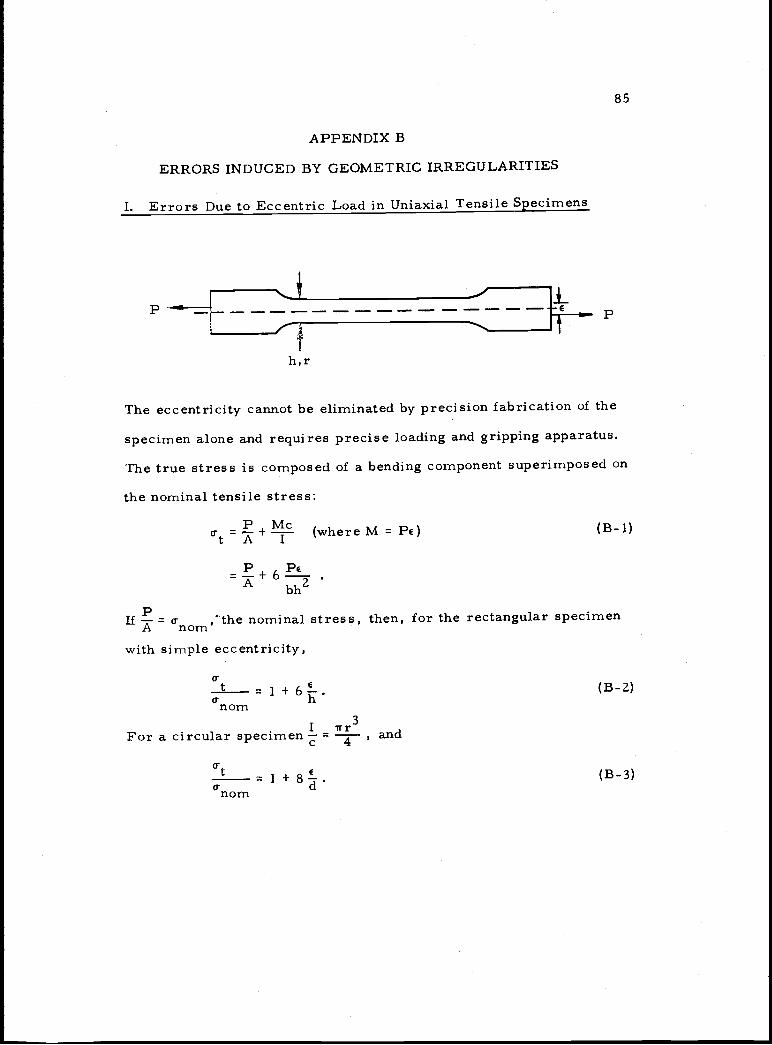
Jh,r
The eccentricity cannot be eliminated by precision fabrication of the
specimen alone and requires precise loading and gripping apparatus.
The true stress is composed of a bending component superimposed on
the nominal tensile stress:
P Mc= + -r (where M = PE) (B-I)
-+ 6-A bh2
If = o ,the nominal stress, then, for the rectangular specimenA nom
with simple eccentricity,
:t =i+6.nom
3I iTrFor a circular specimen = and
:t =I+8.nom
APPENDIX B
ERRORS INDUCED BY GEOMETRIC IRREGULARITIES
I. Errors Due to Eccentric Load in Uniaxial Tensile Specimens
85
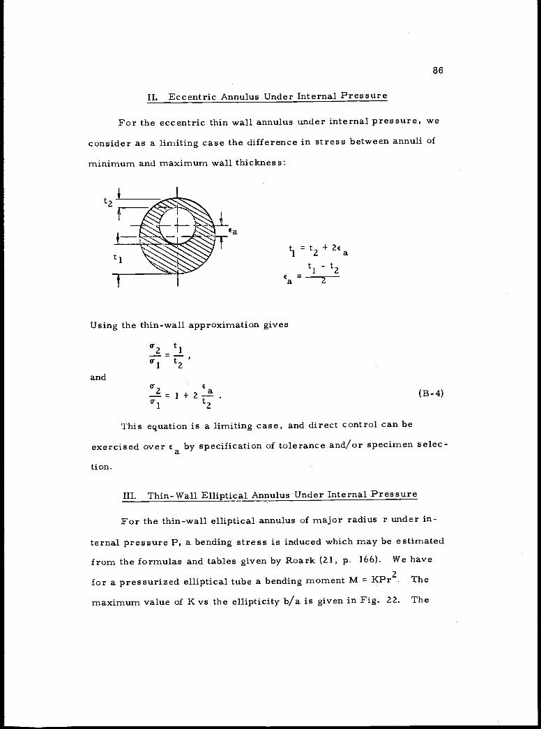
II. Eccentric Annulus Under Internal Pressure
For the eccentric thin wall annulus under internal pressure, we
consider as a limiting case the difference in stress between annuli of
minimum and maximum wall thickness:
t1 = t2
E
-
a 2
86
Using the thin-wall approximation gives
tiO1 t2'
and
= + a taB -4)
This equation is a limiting case, and direct control can be
exercised over Ea by specification of tolerance and/or specimen selec-
tion.
lU. Thin- Wall Elliptical Annulus Under Internal Pressure
For the thin-wall elliptical annulus of major radius r under in-
ternal pressure P, a bending stress is induced which may be estimated
from the formulas and tables given by Roark (21, p. 166). We have
for a pressurized elliptical tube a bending moment M = KPr2. The
maximum value of K vs the ellipticity b/a is given in Fig. 22. The

K
0.3
0.2
0.1
Fig. 21 . Maximum bending coefficient for elliptical tube under in-ternal pressure (after Roark, ref. 21).
0'.4
be
00
M = Kpa2K COEFFICIENTp = INTERNAL PRESSUREa SEMIMAJOR AXIS
b SEMIMINOR AXIS
10.0
J 1.0
0
H=1
z0
U0.1
0.01
0.1 0.2 0.3 0.4 0.5 0.6 0.7ELLIPTICITY, b/a
0.8 0.9 1.0
GLL-611-3265
= FRACTIONAL aerror 6K fERROR = anom
-
Fig. 22. Error in maximum hoop stress in elliptical tube underinternal pressure.
87
6 8 10 12 14 16 18 20
nt (THIN-WALL TUBES)GLL-611 -3266

perturbing stress (for unit width) will be given by
MKPr2t
/
p
If the nominal stress is given by the thin-wall approximation and
equation (B-5) is considered as a perturbation then the ratio of the two
will be an estimate of error:
)pert 6K)/cr' r
'nom
Error = 6K (B-6)
This equation gives the fractional error in stress due to the
presence of bending. This error is plotted in Fig. 23. These equa-
tions are applicable to the thin-wall tubes on1y and represent a maxi-
mum error due to ellipticity.
88
(B -5)

APPENDIX C
EXTREME VALUE AND MEAN VALUE OF THE TRUNCATED,
UNBIASED WEIBULL DISTRIBUTION
The survival probability of a truncated Weibull distribution with
zero bias (a- = 0) is given as the ratio of the initial survival probability
to the survival probability at the truncation point,
S(13)
S( -Ii)
where ui is the normalized proof stress (truncation point) and 13> 4.
If reasoning similar to that of section F-i is followed, the ex-
treme value is found to be identical to that of the nontruncated distri-
bution since the quantity i/s(4) is equivalent to multiplication by a
constant.
The result, then, for the most probable least value of the trun-
cated distribution is
I \1/m(rn-limnJ F(l+l/m)provided that
4< 13".
If 4 does not meet this condition then 4 is the most likely extreme
value.
The reason for this form of the extreme value is that the fre-
quency distribution retains the same mode regardless of truncation
value, until truncation value, 4, exceeds the mode, in which case 4
defines the mode of the truncated distribution. Several ways of detect-
ing the truncation are suggested. The presence and location of an
89

90
inflection point indicate existence and approximate magnitude of a mode.
If the cumulative distribution exhibits no inflection, the slope at the
abscissa leads to an estimate of 4.
Unlike the extreme value, the mean value of the truncated distri-
bution is always a function of 4i. Referring to a sketch of the failure
frequency,
A is the mean after screening (truncating) at .1. The mean value theo-
rem gives
= e (1+1/m)] ce-Pmr1+1/Imdp.JLJ
ANote that
1is relative to the mean value of the initial distribution.
The experimental confirmation of this equation was not within the
scope of the present study. It is clearly easier to predict the conse-
quences of a screening test than to deduce the parameter or the mean
value of the initial distribution. A possibly fruitful approach is to test
several samples of increasing size and plot the predicted and observed
extreme values as a function of the sample size, as in the sketch below:

The asymptotic extreme value observed will estimateAValues of 3 were computed using Tables of the Exponential
Integral* by transforming to
-(1-1/rn)m[1 me +1/m)] ç
m[F(11/)]mm
Ju du
which in standard notation is
A Iix (x).=+- e E(ll/m)m
A graph of the strength improvement due to truncation is shown in
Fig. 23.
g OBSERVED
PREDICTED FOR NON-TRUNCATED CASE
n
91
Pagurova, V. I. Tables of the exponential integral. New York,Pergamon Press, 1961.

2.4
2.2
<ce.
2.00
1
H
HtJ) 1.8-1
uIH
1.6
H
0z 1.4
1.2
1.0
TRUNCATION LEVEL, 4'
92
0.4 0.8 1.2 1.6 2.0 2.4
GIL -61i.11 -326T
Fig. 23. Strength improvement due to truncation of the Weibulldistribution.

APPENDIX D
VARIANCE OF THE UNBIASED, UNTRUNCATED WEIBULL
DISTRIBUTION AND ITS LEAST VALUES
Before computing the variances, it will be found useful to obtain
the integral of the following function:
H(p,n) =
mm= F n,
e'mdp.Here F = F( 1 + 1/rn) and the result will be in terms of the
parameters p and n. Parameter p will depend on the order of the
moment of the distribution which is being computed, and n is the
number of specimens in the sample for which the statistics of the least
values are desired. Note that the behavior of the mean value is ob-
tained when n = 1, that of the extreme value when n the sample size.
In this sense the number of specimens n corresponds to relative
volume, since the least value in n specimens should represent the
strength of the n-sized specimen. If we let
1/rn1
v Fn1 1/rn-i dc,1/rnrnn F1 p/m
Fpn'm
Putting back,
(QC p/rn - 1 1/rn-iH(p,n)pnp/m
e 1/rn d.m Fn
93
(D-1)

Combining,
1 (p+l)/rn.3
eH(p,n)= (p+/mp+1 ornn
The integral is r( +, givingrn /
m (D.-2)H(p,n) (p+l)/m [r(l + 1/rn)]mn
Now the variance of the unbiased, untruncated Weibull Distribu-
tion is given by
a2 = - mean I d3
aswhere the probability density I is given by
Usingrnm-n IS=e
which is the distribution of least values in a sample of size n, gives
for f,
f as mmm rn-i -3 F nnFm e
94
The mean of this density function is at ni/rn and, putting in
(D-3),
CO 2 m ma2 = mnFm
(- - 1/rn) pm-i
eF
We can expand this into three integrals each of which may be
immediately solved by the formula (D-2):
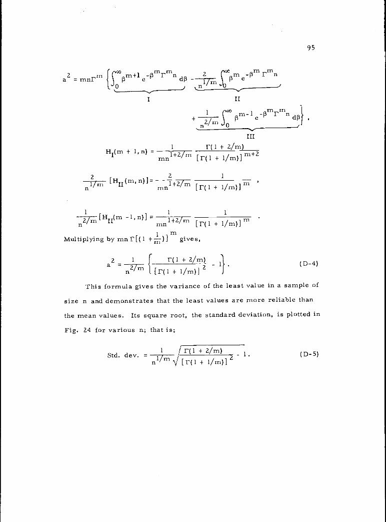
oo rn rn rn rn2 rn rn+1 -3 r n 2 m-f3 F na =rnnF e d3
I II
(bOO rn-i m rn+ 2/mi e
'
H1(m + 1,n) =
21/rn [H11(rn,n)]-
Ti
[H (m -1,n)]= 1+2/rn2/rn II
Ti rnn
Multiplying by rnnF[(1 +)] gives,
2 1 r ['(1+2/rn)a = -i:. (D-4)Z,rn I 2[r(1 + 1/rn)]
This forrnula gives the variance of the least value in a sample of
size n and demonstrates that the least values are more reliable than
the mean values. Its square root, the standard deviation, is plotted in
Fig. 24 for various n; that is:
[r(1 + 1/m)]m
1 F(1+2/rn) -1.+ 1/rn)]
2Std. dev.= i/rn
rn
95
(D- 5)
2 1
rnn1+2/rn [r(1 + 1/rn)]
III1 F( 1 + 2/rn)1 + 2/rn [r(1 + 1/rn)] rn+ 2

1.0
Hz
H
0z0
0. 1U4:
z0H
H
00
z4:H(I)
0.01
96
2 3 4 5 678910 2 3 4 5678910WEIBULL MODULUS, M
Fig. Z4. Standard deviation of various sample sizes as a function ofthe Weibul] modulus.

x S- n na or.n h 1-i
All the other symbols should be self-explanatory. m is Weibull's
modulus, ois stress.
The results may be useful in approximating certain real stress
distributions and providing estimates.
The risk of rupture as computed here is based on the simplified
definition:
R= (-a-) dv.v
APPENDIX E
RISK OF RUPTURE FOR SEVERAL SIMPLE STRESS DISTRIBUTIONS
The risk of rupture is given for several stress distributions. In
the case of the bending stress, an additional condition, static equilib-
rium, has been imposed to provide a comparison between various
distributions which must satisfy this requirement.
A dimensionless length parameter is used by dividing the x-
dimensions by h, the width of the beam. In all cases V is the total
beam volume, i. e., .hb where I is length and b is thickness. The stress
is assumed to be identical over the span I.
97

GLL-6611-3268
STRESS DISTRIBUTION MISC. RISK OF RUPTURE
_x0_x1__-x-r_ X
h
(0rnfII0
GLL-6931 .3269
98
STRESS DISTRIBUTION RISK OF RUPTURE RISK OF RUPTURE K /RR(BENDING) REGION A RA REGION B, RB FOR STA'IC EQUIL.
()m
T()
Tr()
V()I
v(ff)[.1
I1
v()mtl
..II-))m]
(5)m.ISYMMETRIC
(l)1

99
STRESS DISTRIBUTION RISK OF RUPTURE
= KX2
11111"
.
zr;'+Im-F1
v)
aZ 1nm+l(1(_n+lm+1)