Additional Case Study Simulations ofDry Well Drainage in the Tucson Basin

Authors Bandeen, R. F.

Download date 24/05/2018 03:23:02

Link to Item http://hdl.handle.net/10150/306945

ADDITIONAL CASE STUDY SIMULATIONS OF DRY WELL DRAINAGE IN

THE TUCSON BASIN

PREPARED BY:

R. F. BANDEEN

WATER RESOURCES RESEARCH CENTER

UNIVERSITY OF ARIZONA

FINAL REPORT TO

PIMA COUNTY DEPARTMENT OF TRANSPORTATION AND FLOOD CONTROL

DISTRICT

JUNE 1987

..J^1'^ '.

11; ; tARCH Gt;,Nrag

n t;t,IMf

ADDITIONAL CASE STUDY SIMULATIONS OF DRY WELL DRAINAGE IN

THE TUCSON BASIN

PREPARED BY:

R. F. BANDEEN

WATER RESOURCES RESEARCH CENTER

UNIVERSITY OF ARIZONA

FINAL REPORT TO

PIMA COUNTY DEPARTMENT OF TRANSPORTATION AND FLOOD CONTROL

DISTRICT

JUNE 1987

ADDITIONAL CASE STUDY SIMULATIONS OF DRY WELL DRAINAGE IN

THE TUCSON BASIN

TABLE OF CONTENTS

Page

EXECUTIVE SUMMARY 1

INTRODUCTION 2

STUDY OVERVIEW 4

HYDROGEOLOGIC SETTING 5

UNSATURATED FLOW MODELLING OF DRY WELL RECHARGE 7

Storm Water Injection into the Vadose Zone 7

Principles of Flow in the Vadose Zone 8

Unsaturated Hydraulic Conductivity 8

Soil Moisture Retention 9

Specific Moisture Capacity 10

Infiltration 10

Program UNSAT 2 11

Computational Considerations 12

Derivation of Model Input Parameters 13

Relative Hydraulic Conductivity Curves 14

Moisture Retention Curves 14

Specific Moisture Capacity Curves 15

Saturated Hydraulic Conductivity 16

CASE STUDY SIMULATIONS 17

Storm Water Runoff Input to a Dry Well 17

Case 1 Simulation 17

Case 2 Simulation 18

Case 3 Simulation 19

Interpretation of Results 19

Specific Soil Surface 20

DISCUSSION OF RESULTS 22

Case 1 Simulation 22

Storm 1 22

Plume Distribution 23

24 -Hour Drainage Period 24

Storm 2 24

Post -Storm 2 Drainage 25Case 2 Simulation 26

Storm 1 26

Infiltration of Storm Water 26

Distribution of Drainage Plume 2724 -Hour Drainage Period 28

TABLE OF CONTENTS (continued)

Page

Storm 2 29Post -Storm 2 Drainage 30

Case 3 Simulation 31

CONCLUSIONS 33

RECOMMENDATIONS 35

REFERENCES 36

TABLES

Table

1 REPRESENTATIVE VALUES OF SOIL BULK DENSITY ANDSPECIFIC SURFACE

2 ESTIMATED SPECIFIC SURFACE OF SOIL EXPOSEDTO DRY WELL DRAINAGE WATER

ILLUSTRATIONS

Figure

1 RELATIVE HYDRAULIC CONDUCTIVITY CURVE : MATERIAL 1

2 SOIL MOISTURE RETENTION CURVE : MATERIAL 1

3 SPECIFIC MOISTURE CAPACITY CURVE : MATERIAL 1

4 DISTRIBUTION OF WATER CONTENT WITH DEPTHDURING VERTICAL INFILTRATION

5 FINITE ELEMENT GRID

6 RELATIVE HYDRAULIC CONDUCTIVITY CURVE : MATERIAL 2

7 SOIL MOISTURE RETENTION CURVE : MATERIAL 2

8 SPECIFIC MOISTURE CAPACITY CURVE : MATERIAL 2

ACKNOWLEDGEMENTS

The patience of Dave Smutzer, Manager of the Long Range Planning Section, inthe preparation of this report is gratefully acknowledged. Special thanksare extended to Dr. L. G. Wilson of the University of Arizona WaterResources Research Center, Principle Investigator of this Project, for hispatience, technical guidance and assistance through the preparation of thisreport. Special thanks are also extended to Mr. Michael Osborn of the WRRC,Project Manager of this project, for his patience and assistance in thepreparation of this report. Special thanks are extended to Dr. S. P. Neumanand Dr. J. Yeh, Professors of Hydrology at the University of Arizona, fortheir valuable technical consultation on the computer simulations. Theassistance of graduate students Amado G. Guzman, Mariano Hernandez andTimothy P. Leo of the Department of Hydrology and Water Resources,University of Arizona, in performing the computer simulations, is gratefullyacknowledged.

ADDITIONAL CASE STUDY SIMULATIONS OF DRY WELL DRAINAGE

IN THE TUCSON BASIN

EXECUTIVE SUMMARY

Three case study simulations of dry well drainage were performed using

the saturated - unsaturated groundwater flow model UNSAT 2. Each case

simulated injection of storm water runoff water into a dry well from two

five -year, one -hour storm events, separated by a 24 -hour lag period. The

first case assumed subsurface conditions of a uniform gravelly sand material

from land surface to the water table at 100 feet below land surface. The

second case assumed the same gravelly sand, underlain by a uniform

sandy -clay loam material beginning at 30 feet below land surface and

extending to the water table. The third case assumed the same conditions as

in Case 2, except for a sandy loam soil replacing the sandy -clay loam

material. Simulated subsurface flow of injection water for the first case

was primarily vertical. The cross- sectional radius of the 95% saturated

portion of the drainage plume reached a maximum of about nine feet during

stormwater injection. In the second and third cases, horizontal flow took

place at the layer boundary between the gravelly sand and underlying fine

material. As a result, the cross -sectional radius of the 95% saturated

portion of the drainage plume reached a maximum of about 27 feet for Case 2,

and about 21.5 feet for Case 3. Arrival times of injection water at the

water table varied from between 0.25 and 0.75 hours (Case 1) , and between

130 and 150 hours (Case 2). Attenuation of water -borne pollutants in the

vadose zone is related to the degree of exposure of drainage water to soil

particle surfaces. The specific surface area of soil particles to which

drainage water was exposed was used as an indicator of the relative degree

of attenuation that may take place among the three cases. The ratio of

specific surface area of soil matrix exposed to the portion of the sub-

surface reaching a state of 80% saturation was approximately i : 16.2 : 5.6

(Case 1 : Case 2 : Case 3).

1

INTRODUCTION

Concern over dry wells as a source of groundwater pollution in Arizona

has led to state legislation requiring registration of existing and new dry

wells and licensing of dry well drillers (Arizona House of Representatives,

Bill 2229). Pima County and the City of Tucson have both recognized the

need for hydrogeologic studies to be performed on dry wells to aid in the

prediction of groundwater contamination associated with their use. In 1983

Pima County authorized funding for a field tracer study using an experi-

mental dry well at the field station of the University of Arizona Water

Resources Research Center (WRRC), Tucson, Arizona. Results were reported by

Wilson (1983). Subsequently, Bandeen (1984) used the variably saturated

flow model UNSAT 2 to simulate the subsurface flow system generated during

operation of the dry well using a worst -case scenario which assumed that the

well terminated above a completely impermeable geologic stratum. This study

simulated the condition of maximum lateral movement of drainage water. The

work described in this report focuses on the modeling of dry well drainage

of storm water runoff for three additional subsurface conditions:

1. percolation of storm water from a dry well into a highly permeable

zone above a water table;

2. percolation into a zone of highly permeable material underlain by a

sandy clay loam material extending from a depth of 30 feet to the water

table at 100 feet;

3. percolation into a zone of highly permeable material underlain by a

sandy loam material extending from a depth of 30 feet to the water table at

100 feet.

These three case studies illustrate how dry well drainage water

distributes itself through the course of a runoff event for uniform and

layered subsurface conditions representative of the Tucson Basin. Results

of the Wilson (1983) study suggested that subsurface attenuation of

2

pollutants may increase with lateral spreading of drainage water in the

vadose zone. This lateral spreading increases for layered subsurface

conditions in which vertical flow of drainage water is impeded by layers of

low permeability. Where vertical flow is retarded at a transition to a

layer of lower permeability, drainage water mounds up and spreads laterally

along the layer transition. This phenomenon may increase vadose zone

attenuation of pollutants by increasing both the degree and the duration of

exposure of drainage water to vadose zone soil particles. The results of

this study provide an illustrative example of how drainage plume distri-

bution, rate of movement, and, indirectly, degree of attenuation, vary

between uniform and layered soil conditions representative of the Tucson

Basin.

3

STUDY OVERVIEW

Computer simulations of subsurface flow were performed for the three

case studies assuming general hydrogeologic conditions observed at the WRRC

field station. Previous studies by Dumeyer (1966) and Osborne (1969)

indicate that a transition from a zone of relatively high sand and gravel

content to a zone of relatively high silt and clay content exists in the

vicinity of the WRRC experimental dry well at depth of approximately 30 feet

below land surface. The constitution of the more permeable material above

the layer transition at the site was determined from drill cuttings obtained

during construction of the dry well. This highly permeable material is

representative of sediments associated with high energy depositional

environments, such as river channels, in the Tucson Basin. The Case 1

simulation addresses the situation of a dry well draining into a highly

permeable material extending from land surface to the water table at a depth

of 100 feet in order to illustrate rapid and direct infiltration of drainage

water. This transition from a zone of relatively high permeability to a

zone of relatively low permeability at a depth of 30 feet has been observed

to cause the perching of drainage water introduced through the dry well and

the subsequent lateral migration of this drainage water along the layer

transition (Wilson, 1983). Inspection of City of Tucson well logs shows

that abrupt transitions of geologic materials from zones of high hydraulic

conductivity to zones of low hydraulic conductivity is a common occurrence

in the Tucson Basin. As such, the associated phenomenon of perching and

lateral migration of infiltration water, in areas where dry wells drain into

such sediments, is also likely to be common. This hydrogeologic feature was

included in the Case 2 and Case 3 simulations in order to model the phenome-

non of perching and lateral migration of infiltration water. The constitu-

tion of the less permeable hydrogeologic material below the layer transition

for Cases 2 and 3 is representative of subsurface conditions at the WRRC

field site and of common Tucson Basin sediments. These simulations address

the situation of a dry well draining into a highly permeable zone near the

surface which is underlain by a hydrogeologic material of lesser per-

meability, inducing perching and lateral migration of the drainage water.

4

HYDROGEOLOGIC SETTING

Drainage and tracer tests were conducted on an experimental artificial

recharge well at the field laboratory of the WRRC. Dumeyer (1966) charac-

terized the vadose zone sediments at the WRRC field site as a series of

alternating beds of varying sand, silt, clay and gravel composition.

Dumeyer described the vadose zone deposits as consisting of three major

units: Quaternary alluvium on the surface, underlain by Quaternary Basin

Fill, which is in turn underlain by Tertiary sediments. Sieve analysis

performed by Osborne (1969) and neutron logs taken from two -inch diameter

access holes near the dry well indicate that the transition between the

Quaternary Basin Fill and Quaternary alluvium occurs on the average at a

depth of about 30 feet in the vicinity of the field site. Drilling time

logs for access holes in the vicinity of the dry well show peak values in

the zone of 20 to 30 feet below land surface. Longer drilling time

generally corresponds to coarse subsurface materials such as sands, gravels,

and cobbles. The drilling logs also show loss of drilling fluid at these

depths, which is indicative of a zone of highly permeable material. Grain

size distribution analyses performed by Osborne exhibit the following

trends: 1) generally high sand and gravel content from land surface to

30 feet, with maximum gravel content from 20 to 30 feet; and 2) increased

silt and clay content beginning at approximately 25 to 30 feet. Neutron

logs obtained from the access holes during recharge experiments illustrate

an accumulation of water in the zone of 25 to 35 feet and subsequent lateral

movement of the accumulating water (Wilson, 1983). All of these observa-

tions support the conclusion of a stratigraphic transition from a highly

permeable sand and gravel unit to a less permeable loam material at approxi-

mately 30 feet below land surface. This observed field condition serves as

the basis for the layered subsurface conditions assumed in the Case 2 and

Case 3 simulations.

The depth to water at the WRRC field site is approximately 110 feet. A

depth of 100 feet was assumed in the simulations to help optimize the size

5

of the model grid. A depth of approximately 100 feet to groundwater is

representative of many parts of the Tucson Basin.

6

UNSATURATED FLOW AND MODELING OF DRY WELL INJECTION

STORMWATER INJECTION INTO THE VADOSE ZONE

Dry wells are usually designed to inject runoff water into highly

permeable soil materials. The sediments that extend from land surface to

the water table constitute the "vadose zone." Prior to storm water

injection, the vadose zone surrounding a dry well is in a state of residual

saturation. The interstices between the soil grains are partly filled with

water remaining from previous recharge events. The remaining pore space is

filled with air. Sediments in this state are described as "unsaturated."

The water in the interstices of unsaturated soil is subjected to capillary

forces that create a negative pressure or suction within the soil matrix.

When storm water is introduced via a dry well, the air in the soil

interstices is expelled and the sediments around the dry well become

saturated. As the water injected. via the dry well is under the pressure

caused by the weight of water in the dry well shaft, a hydraulic gradient is

generated which causes the water to move into the surrounding unsaturated

sediments. This flow takes place in both the lateral and vertical direc-

tions under the combined effects of the pressure differential and gravity.

In uniform soils, gravity eventually becomes the dominant driving force and

the vertical flow component becomes more pronounced than the horizontal. In

layered soils the downward movement of water may be impeded by beds of

relatively low permeability and the water may spread laterally over consid-

erable distances before resuming downward movement.

As storm water injection continues during and after a precipitation

event, the saturated region below and surrounding the dry well continues to

expand. If the volume of runoff water is sufficient, this saturated region

may eventually extend to the water table. If the volume of runoff water is

relatively small, the front of saturation may remain and possibly stabilize

above the water table.

7

PRINCIPLES OF FLOW IN THE VADOSE ZONE

The rate at which water can be injected into the vadose zone from a dry

well, as well as the manner and rate at which the injected water propagates

through the vadose zone to the aquifer, are determined by the level of water

in the dry well shaft, the initial water content of the surrounding and

underlying soils, and the hydraulic properties of these soils. The rate of

flow through both the saturated and unsaturated regions is controlled by an

equation for flow in porous media known as Darcy's Law. According to

Darcy's Law, the volume of water crossing a unit area of soil in a unit of

time, known as "specific flux," is directly proportional to the rate at

which hydraulic head decreases in the direction of flow per unit distance,

know as "hydraulic gradient." The constant of proportionality, usually

designated by the letter K, is known as "hydraulic conductivity," and has

the same dimensions as velocity. Values of hydraulic conductivity are

typically measured in units of centimeters per second, feet per day and

other related units. Values of hydraulic conductivity for various soil

types vary by several orders of magnitude. Values for hydraulic

conductivity for a clean sand and gravel typically range from 100 feet per

day to 1,000 feet per day. Values for fine sand typically range from 1 foot

per day to 100 feet per day. Values for silt and mixtures of sand, silt and

clay typically vary from 0.001 feet per day to 1 foot per day. Dense clays

generally have hydraulic conductivity of less than 0.001 feet per day (U.S.

Dept. of the Interior, 1977).

Unsaturated Hydraulic Conductivity

Hydraulic conductivity, except for very minor changes resulting from

variations in temperature and fluid density, is a constant property of the

soil and the fluid that penetrates it. In the saturated zone below the

water table, water maintains a relatively uniform temperature so that K

depends solely on the permeability of the soil. In the vadose zone, the

soil pores are filled with both water and air, and K depends on the relative

8

amounts of these two fluids. The higher the water content, expressed as

volume of water per bulk volume of soil, the larger the value of unsaturated

K. Each soil has a functional relationship between unsaturated K and water

content. Just as K varies with water content, so does specific flux. The

process of injection and flow propagation from a dry well depends on the

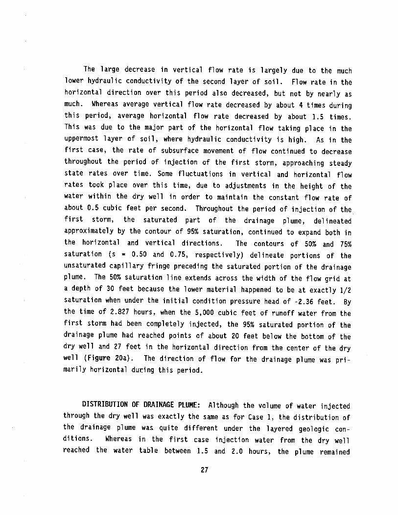
degree of saturation of the soil material. "Relative" hydraulic conductivity

is the ratio between the hydraulic conductivities of a soil under unsatu-

rated and saturated conditions. A graph of relative hydraulic conductivity

versus water content is shown in Figure 1.

When permeability varies from location to location in a given layer of

soil, the soil material is said to be "heterogeneous." When permeability

varies depending on direction at a given location, the soil material is said

to be "anisotropic." Conversely, when soil permeability is constant with

respect to location and direction in a given layer of soil, that soil

material is described as "homogeneous" and "isotropic." The use of layered

subsurface conditions in the Case 2 and Case 3 simulations introduces

heterogeneity and anisotropy between layers. Within the layers themselves,

however, homogeneity and isotropy are assumed.

Soil Moisture Retention

For a soil in a variably saturated state, i.e. undergoing wetting or

drying, there exists a unique relationship between water content and soil

pore pressure. This functional relationship, the graph of which is called

the soil moisture "retention curve," is another property characteristic of a

given soil which controls unsaturated flow in the vadose zone. Generally,

as the water content increases, the negative, or capillary, pressure becomes

less negative. Negative pressure head is also known as "suction head,"

which is plotted as a positive quantity, as in the soil moisture retention

curve shown in Figure 2. Soil retention curves are generally determined

either in the laboratory using a pressure chamber, or in the field using

instrumentation sensitive to soil pore pressure and moisture content.

9

Specific Moisture Capacity

By taking the reciprocal of the slope of the soil moisture retention

curve, a third characteristic unsaturated flow property, the "specific

moisture capacity" of the soil as a function of water content, is obtained.

Specific moisture capacity may be viewed as the volume of water the soil

absorbs per unit decrease in suction. An example of a specific moisture

capacity curve is shown in Figure 3. The specific moisture capacity as a

function of water content is used in calculating mass balance in flow

through unsaturated soil. Mass balance and Darcy's Law are the two physical

principles that underlie most models of groundwater flow through the

subsurface under both saturated and unsaturated conditions. The same

principles form the basis for the variably saturated flow model UNSAT 2 used

in these simulations.

Infiltration

Infiltration is the process by which water from a surficial source

advances underground. It is important to note that infiltrating water does

not penetrate the subsurface in a "plug flow" process where the infiltration

front is marked by an abrupt transition from completely dry to completely

saturated soil. Instead, infiltration is characterized by a condition of

soil saturation just below the water source, which tapers off gradually to

some volumetric water content close to the saturated water content, 0, at

some depth, y, below the surface (Figure 4). Below point y, moisture

content tapers off gradually to the value of "background," or residual

moisture content, On, prevailing in the soil. This zone, where moisture

content decreases from close to saturation to residual moisture content, is

known as the "capillary fringe" of the drainage plume. This advancing

capillary fringe of the drainage plume marks the "infiltration front," which

steadily progresses with time, as shown in Figure 4. Between land surface

and point y, moisture content is at a high degree of saturation but still

below 100% saturation. In the contour plots of saturation illustrating the

10

results of the model simulation, point y is approximated by the level of 95%

saturation, and marks the point of advance of the infiltration front in the

soil below and surrounding the dry well.

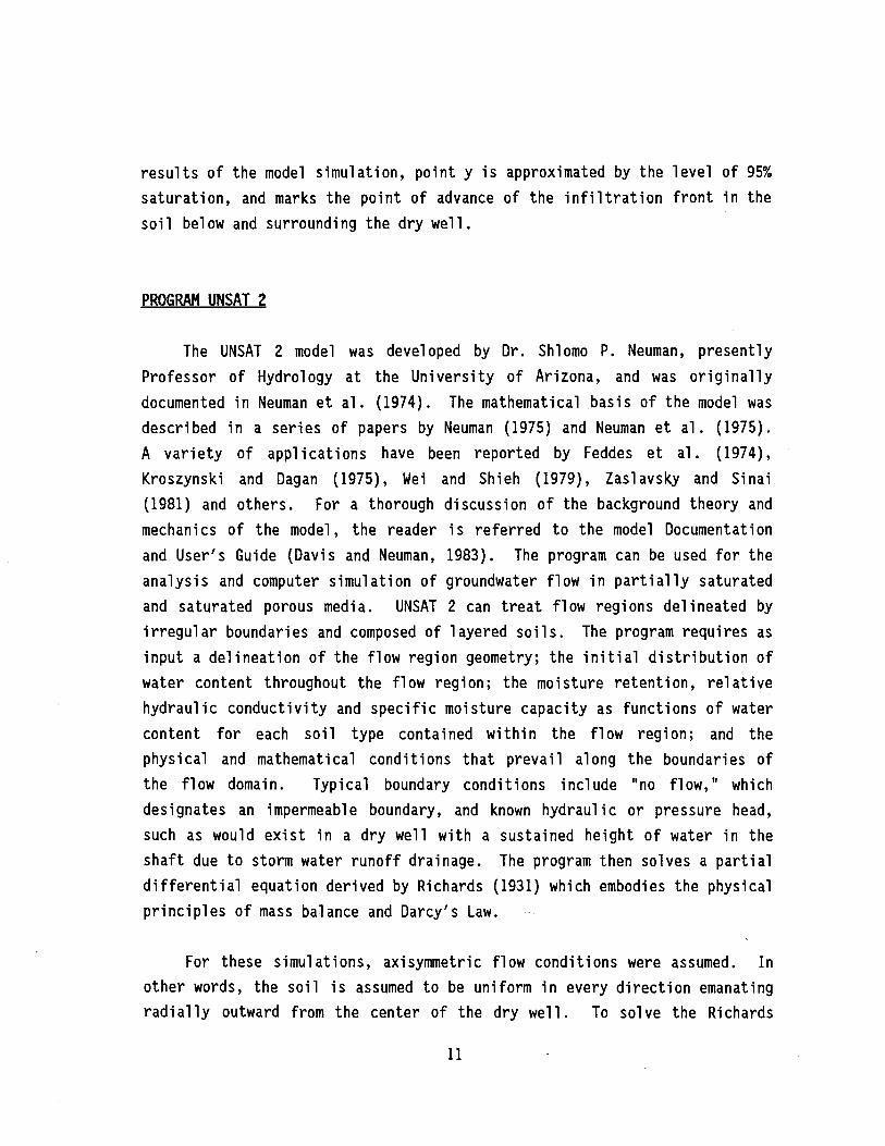
PROGRAM UNSAT 2

The UNSAT 2 model was developed by Dr. Shlomo P. Neuman, presently

Professor of Hydrology at the University of Arizona, and was originally

documented in Neuman et al. (1974). The mathematical basis of the model was

described in a series of papers by Neuman (1975) and Neuman et al. (1975).

A variety of applications have been reported by Feddes et al. (1974),

Kroszynski and Dagan (1975), Wei and Shieh (1979), Zaslaysky and Sinai

(1981) and others. For a thorough discussion of the background theory and

mechanics of the model, the reader is referred to the model Documentation

and User's Guide (Davis and Neuman, 1983). The program can be used for the

analysis and computer simulation of groundwater flow in partially saturated

and saturated porous media. UNSAT 2 can treat flow regions delineated by

irregular boundaries and composed of layered soils. The program requires as

input a delineation of the flow region geometry; the initial distribution of

water content throughout the flow region; the moisture retention, relative

hydraulic conductivity and specific moisture capacity as functions of water

content for each soil type contained within the flow region; and the

physical and mathematical conditions that prevail along the boundaries of

the flow domain. Typical boundary conditions include "no flow," which

designates an impermeable boundary, and known hydraulic or pressure head,

such as would exist in a dry well with a sustained height of water in the

shaft due to storm water runoff drainage. The program then solves a partial

differential equation derived by Richards (1931) which embodies the physical

principles of mass balance and Darcy's Law.

For these simulations, axisymmetric flow conditions were assumed. In

other words, the soil is assumed to be uniform in every direction emanating

radially outward from the center of the dry well. To solve the Richards

11

equation over the flow region, consisting of the soil surrounding and below

the dry well to the water table in the case of this simulation, UNSAT 2 uses

a computational scheme known as the Galerkin finite element method. This

finite element method requires that a radial cross section representing the

flow region be subdivided into a number of triangular or quadrilateral

subregions called elements. The result is a mesh of elements denoted as a

finite element grid (Figure 5). The corners of these triangles and

quadrilaterals are called nodes. The grid represents an area measuring

100 feet horizontally from the center of the dry well, and 110 feet in the

vertical direction. The term "axisymmetric" implies that the actual flow

region simulated is derived by rotating the entire grid 360 degrees about

its left -most border. Using an algebraic approximation to the Richards

equation, the program computes hydraulic heads, pressure heads and water

contents at all the nodes of the finite element grid at progressive points

in time. In these simulations, the initial time is at the onset of

injection into a dry well accompanying a storm event. The solution

progresses forward in time through the first storm event, then through a

24 -hour drainage period, followed by a second storm and subsequent drainage

period. UNSAT 2 also computes the rate of water flow at each boundary node.

From these data one can monitor the total rate of injection for the dry

well.

Computational Considerations

To solve the Richards equation by the finite element method, the

unsaturated soil properties in each element must be known at the beginning

and end of each time increment. In reality, these properties are known only

at the beginning of the time increment. As time progresses, the pressure at

each node changes and this in turn causes a change in the soil parameters of

hydraulic conductivity, water content and specific moisture capacity. These

changes cannot be predicted without knowing the pressures at all the nodes

at the end of the time increment, yet the pressures cannot be computed

without knowing how the soil parameters will change with time.

12

Mathematically, this amounts to having as many unknowns as there are

variables in the equation. To solve for the unknowns in this type of

equation, at the end of each time increment, the soil parameters are updated

to reflect the most recent pressure calculations at all the nodes, and the

solution for the time increment is repeated with these updated values. This

process is repeated for each time increment until the previous and updated

pressure values differ by not more than a user -specified tolerance. The

iterative process therefore provides an approximate solution. A smaller

tolerance implies a more accurate solution, but also implies more computing

time and its associated expense.

As the solution progresses through time, the pressure distribution in the

flow region and its associated moisture content distribution are saved on

separate files for use in creating contour plots. These contour plots give

a graphic representation of the distribution of flow from a dry well at

various stages of storm water recharge events and intermittent drainage.

UNSAT 2 was originally developed for use on an IBM mainframe computer

and was later adapted to CDC and Cyber computers. The program is written in

the ANSI standard Fortran 77 language and is therefore easy to modify for

use on other computers. For these simulations, the Cyber 175 computer at

the University of Arizona was employed.

DERIVATION OF MODEL INPUT PARAMETERS

Three different soil materials were used in these simulations. The

first material constitutes the entire flow region in the Case 1 simulation,

and the zone from land surface to a depth of about 30 feet in the Case 2 and

Case 3 simulations. This material comprises primarily gravelly sand and

sandy gravel, and is called Material 1 for the purposes of this study.

Material 1 is patterned after soil removed from borehole cuttings during

construction of the dry well at the WRRC field site, and is representative

of the soil zone into which the dry well injects water. The second

13

material, Material 2, is patterned after a clay /silt loam type soil

documented in a previous soil study of Tucson Basin soils performed by a

University of Arizona graduate student (Coelho, 1974). The third material,

Material 3, is patterned after a sandy loam type soil documented in a

separate earlier study of Tucson Basin soils by another University of

Arizona graduate student (Guma'a, 1978). All three of these materials are

common in the Tucson Basin and are representative of soils of high (Material

1), low (Material 2), and moderate (Material 3) permeability.

Relative Hydraulic Conductivity Curves

Field and laboratory measurement of relative hydraulic conductivity, as

a function of water content, is a very time -consuming and expensive process.

A computer model developed by van Genuchten (1978) allows for the derivation

of the relative hydraulic conductivity, as a function of water content

curve, from the soil moisture retention curve. The model employs a closed -

form analytical method to relate the shape of the moisture retention curve

to the inferred shape of the relative hydraulic conductivity curve. This

model was employed for all three of the soil materials used in the simula-

tion to produce the relative hydraulic conductivity curves shown in

Figures 1, 6, and 9.

Moisture Retention Curves

The moisture retention curve, which specifies the relationship of

negative pressure head, or suction head, to water content in the soil, was

obtained using laboratory methods for Material 1, and using in situ and

laboratory methods for Materials 2 and 3 (Coelho, 1974, and Guma'a, 1978).

A special adjustment which accounts for the presence of gravel and cobbles

was made to the Material 1 curve using the method of Bouwer (1984). A

spline function curve -fitting program was used to smooth and fit the curves

14

to laboratory and field data. The moisture retention curves for Materials 1

through 3 are shown in Figures 2, 7, and 10.

The moisture retention curves for a given soil vary in accordance with

whether the soil is being wetted or is draining. This phenomena is known as

hysteresis. Generally, for a given suction head, water content in the soil

will be greater during drying than during wetting. The moisture retention

curves used in this study represent the main drying soil moisture retention

curve for each of the three soil materials. Insofar as the computer model

used in the simulations does not address the phenomenon of hysteresis, its

effects were not considered in this study.

As a result, some discrepancy between the moisture content predicted by

the model, and that actually occurring for a given soil material in the

field, is likely to occur during the wetting (storm water recharge) phase of

the simulations. In using a drying moisture retention curve to simulate a

wetting condition, soil water content for a given suction head will be

slightly overestimated during the wetting phase of the simulation. As such,

relative hydraulic conductivity will also be slightly overestimated (for the

wetting phase), resulting in a higher rate of movement of recharged water

during the wetting phase. Consequently, the predicted rates of vertical and

horizontal movement of recharge water during a recharge event will err

slightly to the high side.

Additional laboratory work, to define the main wetting loop of the soil

moisture retention curve using an improved model for each material, and

additional model simulations would have to be conducted to incorporate the

hysteretic effects of the soil.

Specific Moisture Capacity Curves

The relationship of specific moisture capacity to water content for the

three soils was obtained using a computational routine in the UNSAT 2

15

program which calculates the inverse of the slope of the moisture retention

curve at various values of water content. The spline algorithm routine was

employed to smooth the curves. The specific moisture capacity curves are

shown in Figures 3, 8, and 11.

Saturated Hydraulic Conductivity

UNSAT 2 was used to simulate conditions observed in the dry well tracer

tests performed by Wilson (1983) to calibrate a value for saturated

hydraulic conductivity, known as Ks. This was accomplished by using known

dry well inflow rates from the field tests and measurements of the height of

water in the dry well shaft. The field- measured height of water in the dry

well shaft for a given recharge test was specified as a boundary condition

in the model. The assumed value for Ks was then varied through a series of

experimental computer runs until the inflow rate into the dry well, as

computed by the model, matched the inflow rate observed in the field. The

resulting calibrated Ks for Material 1 was 6.7 feet per hour, or about

161 feet per day. The Ks values for Materials 2 and 3 were calculated using

field and laboratory methods. The values of Ks for Materials 2 and 3, as

reported by Coelho and Guma'a, were 0.29 feet per hour and 1.0 feet per

hour, respectively.

16

CASE STUDY SIMULATIONS

STORM WATER RUNOFF INPUT TO A DRY WELL

Runoff for a five -year, one -hour storm, calculated specifically for the

Tucson Basin from a Soil Conservation Service standard hydrograph, was used

as input for the dry well in all three simulations. The influx of storm

water from this precipitation event was input to the model twice, separated

by a 24 -hour lag period. This simulates the effect of multiple storms, such

as those that may occur almost daily in the Tucson area during the monsoon

season. The volume of runoff from this storm was calculated as

approximately 5,000 cubic feet. The manufacturer of the experimental dry

well at the WRRC field station indicated that over the long term, most dry

wells are designed to accommodate a flow of approximately 0.5 cubic feet per

second (cfs). Though this intake rate varies with the size, age and quality

of runoff water for specific dry wells, the rate of 0.5 cfs was specified by

the manufacturer as the expected long -term intake rate for a Maxwell Type

III dry well servicing one paved acre (De Tommasso, 1984). With this in

mind, the rate of dry well recharge was controlled during each simulation to

average about 0.5 cfs for the duration of each of the storm recharge events.

Using this criterion, the 5,000 cubic feet of run -off for each of the 5-

year, 1 -hour storms was recharged for about 10,000 seconds, or 2.77 hours.

CASE 1 SIMULATION

The first case study was a hypothetical simulation that assumed a flow

region made up entirely of Material 1 soil. Actual field data show that

soil similar to Material 1 in texture and hydraulic properties exists only

to a depth of about 30 feet. However, in areas of the Tucson Basin where

river channel deposits prevail, it is common for these materials to exist in

depth intervals of 100 feet or more. The Case 1 simulation was designed to

address the situation where the entire vadose zone is composed of a highly

17

permeable material. This simulation of dry well drainage was expected to

show, relative to the other two, a maximum rate of vertical infiltration, a

minimum time of arrival of drainage water at the water table, and a minimum

cross -sectional area of the drainage plume, allowing for a minimal amount of

attenuation of contaminants potentially contained in the runoff water.

Attenuation of water -borne contaminants in the vadose zone constitutes a

"filtration" of water by the soil, and includes such processes as

adsorption, ion- exchange, complexation and precipitation. By limiting the

surface area of soil particles to which the water is exposed, and the time

of that exposure due to rapid infiltration, these processes will be at a

minimum in the Case i simulation. Essentially, the Case 1 simulation

depicts the worst case of the three with regard to the likelihood of

groundwater contamination via the dry well.

CASE 2 SIMULATION

The second case study incorporates the concept of a layered flow

region, as observed at the WRRC field station site. In this case, the zone

extending from land surface to a depth of 30 feet consists of Material 1,

and the remainder of the flow region from 30 feet below land surface to the

water table consists of Material 2. Lithologic data at the field site

indicate that the zone below 30 feet is actually composed of loam material

with varying degrees of sand, silt and clay. The Case 2 simulation assumes

the uniform existence of the Material 2 sandy clay loam below 30 feet. The

existence of a soil material transition from a material of relatively high

permeability (Material 1) to a material of relatively low permeability

(Material 2) at 30 feet causes a retardation of downward movement of

drainage water and, as more water builds up at this transition, lateral flow

along the material transition. This case study provides a contrast to the

Case 1 study in that the plume of drainage water emanating from the dry well

is forced to percolate through a material of much lower permeability and

therefore moves much more slowly. Furthermore, by spreading out laterally

along the material transition, the plume of drainage water is distributed

18

over a much larger area, exposing it to a much larger proportion of soil

material. As a result, water -borne constituents in the dry well influent

undergo a much greater proportion of the attenuation processes associated

with the soil material. The greater cross -sectional area of the plume of

drainage water implies a greater opportunity for dilution of drainage water

with the groundwater when the drainage water percolates to the water table.

In this case, relative to the other two, rate of downward infiltration will

be at a minimum, time of arrival of drainage water at the water table will

be at a maximum, and the degree of available soil surface area for attenua-

tion will be at a maximum. The Case 2 simulation depicts the scenario where

dry well- associated groundwater contamination is least likely to occur.

CASE 3 SIMULATION

The third case study was designed to present an intermediate case in

comparison to the other two. As in Case 2, a layered condition is assumed,

but the soil material below a depth of 30 feet to the water table comprises

Material 3, a sandy loam. Also, as in Case 2, the soil extending from land

surface to a depth of 30 feet comprises Material 1. The results were

expected to be similar to those of Case 2, except that the degree of lateral

spreading at the material transition is not as great, and the rate of

infiltration to the water table is somewhat greater. The Case 3 simulation

is necessary to provide a moderate contrast to the other two, more extreme

cases; it is also representative of soil conditions at the WRRC field site

and in the Tucson Basin in general.

INTERPRETATION OF RESULTS

At specified times throughout the simulations, information concerning

the location and pressure head of all points in the grid was recorded for

use in a contour mapping routine at a later time. At each specified point

in time, contour maps of the degree of saturation and hydraulic head

19

distributions throughout the flow field were plotted. The "degree of

saturation" of a portion of soil is simply the ratio of its given volumetric

water content to its volumetric water content at saturation. Contours of

the degree of saturation for the soil surrounding the dry well provide a

visual representation of the distribution of subsurface water introduced via

the dry well. The "hydraulic head" is a measure of the total potential and

kinetic energy of a particle of fluid at a given point in time. For

infiltration of water in soils, where fluid velocities are relatively small,

the majority of this energy is potential. The hydraulic head consists of

the sum of the pressure head and the elevation of a given fluid particle

above a pre- determined datum. The distribution of hydraulic head in the

flow region determines the flow paths of the drainage water. Each of the

contour plots represents a two -dimensional distribution of saturation or

hydraulic head throughout the finite element grid, which represents an

axisymmetric slice of the area surrounding the dry well. The true

representation of saturation or hydraulic head is obtained by rotating the

plot 360 degrees about its left -most axis, representing the center of the

dry well. The horizontal dimensions of the contour plots vary from 50 to

100 feet.

Specific Soil Surface

The size of the saturated portion of the drainage plume is an indica-

tion of the total surface area of soil particles to which the drainage water

is exposed. The geochemical processes that cause soil to act as a "filter"

for some water -borne contaminants such as ion exchange and adsorption, are

directly related to the degree of exposure of water to soil particle

surfaces (Hillel, 1971). As the radius of the drainage plume increases, so

does the degree of exposure of the water to soil particles and their

associated attenuation and filtration mechanisms.

For comparing the relative degree of exposure of drainage water to

vadose zone soil particles, the maximum soil surface area contained within

20

the region of 80% saturation was estimated for each of the three cases.

These estimates provide a measure of the relative degree of attenuation that

may be expected to take place between the three cases. First the total bulk

volume of soil within the zone of 80% saturation is calculated, assuming an

approximate geometric shape of the drainage plume (i.e. some combination of

circular cylinders, cones and spheroids).

21

DISCUSSION OF RESULTS

CASE 1 SIMULATION

Storm 1

From the beginning of injection to a time of 0.25 hours, the zone of

95% saturation had moved from the bottom of the dry well at a depth of

23.5 feet to a depth of about 36 feet below land surface (Figure 12a). The

rate of infiltration was initially high due to the dry condition of the

soil, which caused a large pressure head gradient between the dry well

injection water, under a positive pressure, and the surrounding soil, under

a negative pressure. As time progressed, the soil zone below a depth of

36 feet remained "unsaturated," but reached ever higher degrees of satura-

tion. The downward progress of infiltration water is illustrated by the

s = 0.95 contour, where soil is very close to saturation. From 0.5 hours to

1.0 hours, the average downward velocity of the soil zone equal to or

greater than 95% saturation was about 21.75 feet per hour. From 1.0 to

1.5 hours, this velocity decreased to an average of about 17 feet per hour.

Generally, the average vertical velocity of infiltrating water will continue

to decrease until rate of advance reaches a stable deep percolation rate.

The deep percolation rate is calculated as the hydraulic conductivity

divided by the water -filled porosity of the soil (Kirkham and Powers, 1.984).

In this case, the zone of 95% saturation reached the water table at 100 feet

below land surface between 1.5 and 2.0 hours after the beginning of injec-

tion (Figure 13a).

The water table is defined as the line of zero pressure head at a depth

of 100 feet, marking the saturated surface of the regional aquifer. From a

time of 2.0 hours to 2.722 hours, the contours of degree of saturation

remained approximately the same. At a time of 2.722 hours of infiltration

22

at the design flow rate of 0.5 cfs, the entire volume of runoff from the

first storm event had been injected through the dry well.

The total hydraulic head distribution for the flow region at the end of

injection of storm water from the first storm is shown in Figure 17a. The

dashed lines represent the approximate flow path of the injected water

moving out from the dry well into the vadose zone. These flow paths

consistently follow lines perpendicular to line of equal head. Due to a

pressure gradient induced by the weight of the column of water in the dry

well, some horizontal flow of water takes place near the dry well. Below a

depth of about 30 feet, the flow direction is predominantly vertical. As

mounding occurs at the water table directly beneath the dry well, the weight

of mounding water induces a pressure gradient in the saturated zone below

the water table, again inducing horizontal flow.

PLUME DISTRIBUTION: Throughout the period of injection of storm water

from the first storm, the radius of the saturated portion of the drainage

plume emanating from the center of the dry well reached a maximum of about

7.75 feet from the center of the dry well. This maximum occurred at a depth

of about 30 feet below land surface. As the drainage plume approached the

water table, this radius became smaller. The radius of the 95% saturated

portion of the drainage plume was at a minimum of about 5.5 feet above the

water table. This narrowing of the cross -sectional area of the drainage

plume with depth was a function of the relatively high velocity of vertical

movement of drainage water.

Taking the 80% saturated portion of the drainage plume to be approxi-

mately the shape of a right circular cylinder of average radius 10.5 feet

and height 83.5 feet (the distance from the top of the column of water in

the dry well to the water table), the total volume of soil bulk contained

within the region of 80% saturation was approximately 29,000 cubic feet.

Following the method of White (1979), this corresponds to a total soil

surface area of about 2.777514 x 10 square meters for soil Material 1.

23

24 -Hour Drainage Period

Following the termination of inflow of storm water after 2.72 hours,

water injected into the soil via the dry well during the first storm drained

downward toward the water table. Flow during this phase of the simulation

was entirely unsaturated by a time of 2.0 hours after cessation of injection

from the first storm (Figure 13c). The position of the saturation = 0.80

contour illustrates this downward movement of residual drainage water over

time. From a time of 2.0 to 9.0 hours of post -storm 1 drainage, the s = 0.80

contour moves from a level of about 70 feet above the water table to about

29 feet above the water table. By the time of 15 hours of drainage, the soil

moisture in the zone of 80% saturation has drained to about 10 feet above

the water table (Figure 14c). From 15.0 to 24.0 hours of post -storm 1

drainage, the saturation distribution in the flow region changes very little

(Figures 14c and 15a). As the residual moisture in the soil at this point

is under a higher soil suction, movement through the soil takes place much

more slowly.

Storm 2

The 24 -hour drainage period was immediately followed by injection of

storm water from a second five -year, one -hour storm. The saturation plot

for the time of 15 minutes of injection of water from the second storm

indicates that the zone of 95% saturation advanced to a level of about 51

feet below land surface, about 15 feet further than for the same period

during storm 1 (Figure 15b). This resulted in a higher downward flow

velocity than that of the first 15 minutes of injection for the first storm.

This higher rate of deep percolation is due to the higher level of moisture

in the soil. The background soil water content in the soil during injection

of the first storm runoff was about 13 %, corresponding to a level of

saturation of 43 %. The background moisture of the soil at the beginning of

injection of runoff from the second storm ranged from about 18% to 23 %,

corresponding to a level of saturation of about 60% to 75 %. The higher

24

background water content was due to moisture retained in the soil from

infiltration of runoff water from the first storm. The higher background

moisture content gave rise to a higher hydraulic conductivity for the soil

below the dry well. By a time of 0.75 hours of injection of storm water

from the second storm, the flow region had a saturation distribution similar

to that at a time of about 2.0 hours during the first storm. From a time of

0.75 hours to 2.66 hours of storm water injection, the distribution of

saturation remained essentially the same (Figures 15c and 16a). The total

time of injection of runoff from the second storm was less than that for the

first storm, again because of the higher initial rates of infiltration.

The distribution of hydraulic head in the flow region at the end of

injection of water from the second storm is similar to that at the end of

the first storm (Figure 17b). Note that higher values of hydraulic head

existed in the saturated zone below the water table at the end of injection

from the second storm. At that point, 10,000 cubic feet of water had been

injected, and additional mounding at the water table had caused a greater

pressure buildup due to the added weight of the mounded drainage water.

This added pressure again induced horizontal flow below the water table, as

shown by the flow lines in Figure 17b.

Post -Storm 2 Drainage

During the period of drainage following the second storm, flow in the

system was predominantly unsaturated flow. At a time of 0.5 hours following

the influx of the 5,000 cubic feet of runoff from the second storm, the zone

of 95% saturation had already dissipated into the regional ground water

system (Figure 16b). The majority of the flow region at that time was in a

state of between 75% and 95% saturation. Though no saturated areas remained

in the vadose zone, a considerable amount of moisture remained bound in the

soil pores. Throughout the first six hours of drainage, the portion of the

flow region characterized by water under a saturation of 80% moved downward

at a rate of approximately five to six feet per hour. At a time of 12 hours

25

of post -storm 2 drainage, this portion of the flow region had advanced to

approximately 10 feet above the water table (Figure 18a). At a time of 24

hours of post -storm 2 drainage, this portion of the flow region was com-

pletely assimilated by the regional ground water system. Typically, given

sufficient time, the soil will reach a characteristic minimum moisture

content, having undergone the maximum possible degree of drainage by

gravity. This minimum level of soil moisture is known as "field capacity."

CASE 2 SIMULATION

The main difference in the Case 2 simulation was the existence of a

second, less permeable soil material beginning at a depth of 30 feet below

land surface. It was expected that, to some degree, this layer would cause

an obstruction to downward flow of drainage water, which would build up at

this layer transition and spread out laterally.

Storm 1

INFILTRATION OF STORM WATER: Figure 19 illustrates the distribution of

saturation in the flow region for the first two hours of injection of the

first storm. By the time of 0.5 hours of injection, water had already

reached the layer transition at 30 feet and begun infiltrating into the

second, less permeable layer. As the vertical flow was retarded by the

abrupt decrease in permeability, horizontal flow took place along the

material boundary. Over the time period of 0.25 to 0.5 hours of injection,

the average rate of vertical flow was approximately 7.7 feet per hour. As

in Case 1, the high initial rates of flow were due to the high pressure

gradients that result when water under pressure is introduced into a

relatively dry porous medium. By a time of 0.5 hours, flow rate in the

vertical direction had decreased substantially.

26

The large decrease in vertical flow rate is largely due to the much

lower hydraulic conductivity of the second layer of soil. Flow rate in the

horizontal direction over this period also decreased, but not by nearly as

much. Whereas average vertical flow rate decreased by about 4 times during

this period, average horizontal flow rate decreased by about 1.5 times.

This was due to the major part of the horizontal flow taking place in the

uppermost layer of soil, where hydraulic conductivity is high. As in the

first case, the rate of subsurface movement of flow continued to decrease

throughout the period of injection of the first storm, approaching steady

state rates over time. Some fluctuations in vertical and horizontal flow

rates took place over this time, due to adjustments in the height of the

water within the dry well in order to maintain the constant flow rate of

about 0.5 cubic feet per second. Throughout the period of injection of the

first storm, the saturated part of the drainage plume, delineated

approximately by the contour of 95% saturation, continued to expand both in

the horizontal and vertical directions. The contours of 50% and 75%

saturation (s = 0.50 and 0.75, respectively) delineate portions of the

unsaturated capillary fringe preceding the saturated portion of the drainage

plume. The 50% saturation line extends across the width of the flow grid at

a depth of 30 feet because the lower material happened to be at exactly 1/2

saturation when under the initial condition pressure head of -2.36 feet. By

the time of 2.827 hours, when the 5,000 cubic feet of runoff water from the

first storm had been completely injected, the 95% saturated portion of the

drainage plume had reached points of about 20 feet below the bottom of the

dry well and 27 feet in the horizontal direction from the center of the dry

well (Figure 20a). The direction of flow for the drainage plume was pri-

marily horizontal during this period.

DISTRIBUTION OF DRAINAGE PLUME: Although the volume of water injected

through the dry well was exactly the same as for Case 1, the distribution of

the drainage plume was quite different under the layered geologic con-

ditions. Whereas in the first case injection water from the dry well

reached the water table between 1.5 and 2.0 hours, the plume remained

27

56.25 feet above the water table at the end of the first storm in Case 2.

In addition, the diameter of the plume was much larger, exposing the injec-

tion water to a much greater area of soil.

By performing a volume and soil particle surface area calculation below

the dry well similar to that in Case 1, the specific soil surface contained

within the maximum area of 80%o saturation was calculated. The total

specific surface of the soil particles to which drainage water was exposed

in Case 2 was estimated to be 4.503878 x 10" square meters, about 16.2 times

that for Case 1. Two main factors contributed to the greatly increased

specific surface of vadose zone soil particles for Case 2: 1) the larger

radius of the drainage plume, and 2) the larger specific surface of the

finer soil particles constituting the second material. Furthermore, because

the soil material below 30 feet was much less permeable than Material 1, the

slower rate of infiltration allowed more time for adsorption to take place.

24 -Hour Drainage Period

Figures 20b through 22a illustrate the distribution of flow parameters

for the 24 -hour drainage period separating the two storms. These figures

show the downward percolation and gradual dissipation of the saturated

portion of the drainage plume left over from the first storm. During the

first hour of drainage, the vertical flow rate of the saturated plume con-

tinued to diminish. Over the time periods extending from the end of the

first storm to 0.25, 0.50 and 1.0 hours of drainage, the vertical flow rate

was 3.78 feet per hour, 2.09 feet per hour and 1.766 feet per hour,

respectively, judging from the progression of the zone under 95% saturation.

From the time of 1.5 to 2.0 hours of drainage, the average vertical flow

rate was 1.0 feet per hour. Figures 21b and 22a show little change in the

plume configuration from 5.5 hours of drainage to 24 hours of drainage,

indicating a very low rate of flow through the low- conductivity sandy clay

loam material.

28

Storm 2

The vertical and horizontal movements of the drainage plume through the

period of injection of the second storm were very similar to those of the

first storm. Both horizontal and vertical flow rates were higher during

this period due to the higher soil moisture in the area surrounding the dry

well, a result of injection of water from the first storm. As a result,

soils in the area around and below the dry well took on a higher hydraulic

conductivity. As in the first storm, both horizontal and vertical rates of

advance for the drainage plume decreased with time throughout the period of

injection, though they remained consistently higher than in the first storm

due to the higher background moisture. Between 1.25 hours and 1.75 hours of

injection, average vertical flow rate was 7.7 feet per hour and average

horizontal velocity was 4.7 feet per hour. By the time of 1.75 hours of

injection, the contour of 95% saturation, moving progressively further down

with the advance of the infiltration front, had nearly assimilated the small

region of 95% saturation remaining in the soil below the dry well from the

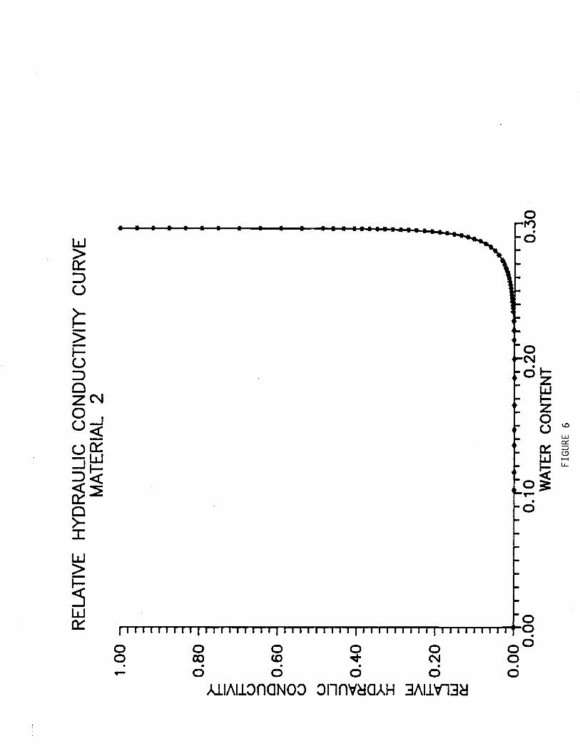
first storm (Figure 23b). By the time of 2.629 hours of injection, the time

required to inject 5,000 cubic feet of water from the second storm, the

saturated portion of the drainage plume had reached a point 45.8 feet above

the water table, approximately 10.5 feet further down than it was at the end

of injection from the first storm (Figure 24a). At this time the plume

reached a distance horizontally from the center of the dry well along the

layer transition of about 33.5 feet, only about a foot farther than it was

after injection from the first storm. Thus, it appears that during the

second storm, the proportion of vertical to horizontal flow of drainage

water was greater than during the first storm. This may be attributed to

the higher moisture content of the soil prior to injection, allowing for

more vertical gravity drainage and resulting in less perched water at the

layer transition and subsequent lateral flow.

29

Post -Storm 2 Drainage

Up until about two hours following the end of injection from the second

storm, portions of this region remained saturated. Downward flow rate of

the saturated portion of the plume averaged about two feet per hour during

this time. Beyond approximately two hours following the second storm, the

entire flow region was unsaturated, though a large portion of it remained in

a state of 90 -95% saturation up to a time of 130 hours following the second

storm.

From a time of 9.0 hours to 286.0 hours following Storm 2, the slow,

downward percolation of drainage water can be monitored through the movement

of the saturation contours (Figures 25 through 27). From 3.0 hours

following Storm 2 on, the zone of 90% saturation advanced at rates of less

than one foot per hour. Between 84 and 130 hours following the second

storm, the rate slowed to less than 0.1 foot per hour. By a time of

262 hours after the second storm, the contour of 80% saturation reached the

water table (Figure 27). At a time of 286 hours following the storm, the

distribution of saturation in the flow region had changed only slightly.

Generally speaking, gravity drainage will continue at this slow rate until

all of the water under 80% saturation has been assimilated into the aquifer.

Given time, the water under 70% saturation will also be assimilated.

Gravity drainage will continue until the soil reaches field capacity,

whereupon negative pressure (suction) forces in the soil bind the water, and

percolation rates become very small. Figure 28a illustrates the distri-

bution of hydraulic head for the first storm of Case 2. The flow lines

illustrate the effect of a horizontal component of flow developing at the

layer transition at 30 feet over time. Flow moves laterally along the layer

transition until it resumes a primarily vertical path of infiltration toward

the water table, upon penetrating the clay loam layer. The flow paths shown

at a time of 1.66 hours of injection from the first storm are essentially

the same as those at the end of the injection period (Figures 28b and 29a).

The flow paths observed at the end of the second storm show essentially the

30

same configuration as those at the end of the injection period for the first

storm (Figure 29b).

CASE 3 SIMULATION

The distribution of soil saturation throughout the period of injection

of a five -year, one -hour storm and subsequent drainage period in the third

case is similar to both Cases 1 and 2, but represents an intermediate stage

of moisture distribution in comparison to Cases 1 and 2. The saturated

hydraulic conductivity of the soil material underlying the layer transition

in this case was 1.0 foot per hour, less than that of the same zone for Case

1, and greater than that of the same zone for Case 2. As one would expect,

some lateral migration of drainage water occurred at the layer transition,

but not to the same degree as in the second case (Figures 30a through 3Oc).

The rate of downward movement of drainage water to the water table following

injection of storm water was higher than that for Case 2, due to the higher

hydraulic conductivity of the soil material. The zone of 90% saturation

contacted the water table some time between 3 and 5 hours, compared to over

130 hours in Case 2 (Figures 31c and 32a).

A volume and surface area calculation similar to that used in the other

two cases was performed. The total surface area of soil particles to which

drainage water is exposed in this case was estimated at 1.570927 x 10"

square meters (Table 2), roughly 25 times that for Case 1, and slightly more

than a third of that for Case 2.

The distribution of hydraulic head for the flow region during storm

water injection for Case 3 illustrates the development of a horizontal

component of flow with time, as in Case 2 (Figure 33). The flow paths do

not extend outward radially as far as in Case 2, however, due to the higher

hydraulic conductivity of the sandy loam below the layer transition.

31

The third simulation was terminated at the end of the 24 -hour drainage

period following injection of storm water from the first storm due to the

development of a numerical problem with the computer program in the

beginning stages of injection of water from the second storm. At this

point, the computer program began to predict excessively high levels of

water at the water table, inconsistent with the amounts of water that had

been injected during the first storm. It is believed the problem was caused

by some numerical instability associated with the unusually dry soil

condition used as an initial condition for the model. Judging from the

previous two cases, simulation of injection of storm water from only one

storm is adequate for the assessment of flow rates, flow paths and exposure

to soil particle surfaces in the vadose zone.

32

CONCLUSIONS

The direction of flow in Case 1 was primarily vertical. Vertical flow

velocities were highest at the beginning of an injection event, and

decreased steadily up until the time of contact with the regional aquifer.

Contact of injection water with the regional aquifer was made between 1.5

and 2.0 hours of injection. The specific surface for the soil particles

contained about 2.777514 x 1010 square meters. Vertical flow velocities

were higher during injection from the second storm event than during

injection from the first storm event, due to a higher initial degree of

saturation and relative hydraulic conductivity. Contact of injection water

with the regional aquifer was made between 15 minutes and 45 minutes of

injection from the second event. The dimensions of the drainage plume

remained essentially unchanged during the second storm injection event.

In Case 2, perching of injection water along the layer transition at

30 feet induced lateral components of flow along the layer transition. The

95% saturated portion of the drainage plume reached a maximum horizontal

distance of about 27 feet from the center of the dry well during the first

injection event. This distance increased to about 32 feet during the second

injection event. The time required for the 90% saturated portion of the

drainage plume from both injection events to reach the regional water table

was between 130 and 150 hours. The specific surface of soil particles

included in the largest area of 80% saturation during the simulation was

about 4.503878 x 10" square meters.

Horizontal flow occurred along the layer transition during injection

events for Case 3 also, but to a lesser extent than in Case 2. The maximum

extent of horizontal movement of the 95% saturated portion of the drainage

plume during the first injection event was about 21.5 feet from the center

of the dry well. Vertical flow velocities of injection water were lower

than in Case 1 and higher than in Case 2. Injection water from the first

event contacted the regional aquifer between 5.5 hours and 6.25 hours after

the start of injection. Specific surface area of soil particles included

33

within the maximum extent of the zone of 80% saturation was about 1.570927 x

10" square meters.

34

RECOMMENDATIONS

1. Dry wells should not be placed in areas where subsurface conditions

are characterized by uniform, highly permeable soil materials between the

dry well and the water table. Drainage via dry wells into this type of

subsurface environment allows for a minimum of attenuation of water -borne

pollutants in the vadose zone.

2. Dry wells should be placed in areas where subsurface conditions are

characterized by multi -layered soil materials, some of which are predomi-

nantly clay in composition. Drainage via dry wells into this type of

subsurface environment allows for a maximum of attenuation of water -borne

pollutants in the vadose zone.

3. Strict regulation of the location of dry wells and of all materials

entering dry wells should be applied. The distance of about 75 feet between

the bottom of the dry well and the water table assumed in this study is

sufficient for some attenuation of pollutants in the drainage water to take

place. However, even under the most favorable subsurface conditions,

attenuation of contaminants in the vadose zone may be incomplete.

35

REFERENCES

Bandeen, R. F., 1984. Case Study Simulations of Dry Well Recharge in theTucson Basin. Completion Report to Pima County Department of Trans-portation and Flood Control District.

Bouwer, H., and R. C. Rice, 1984. "Hydraulic Properties of Stony VadoseZones," Ground Water, Vol. 22, No. 6.

Buckman, H. O., and N. C. Brady, 1969. The Nature and Properties of Soils.Macmillan, New York, 1969.

Coelho, M. A., 1974. Spatial Variability of Water Related Soil PhysicalProperties. Ph.D. Dissertation, University of Arizona, Tucson,

Arizona.

Davis, L. A., and S. P. Neuman, 1983. Documentation and User's Guide:UNSAT 2 - Variably Saturated Flow Model. Water, Waste and Land, Inc.Prepared for the U.S. Nuclear Regulatory Commission, NUREG /CR -3990,

WWL /TM- 1791 -1.

De Tommasso, S.C., McGuckin Drilling, Inc., Phoenix, Arizona, June 1984.Personal Communication.

Dumeyer, J. M.ResearchArizona,

Feddes, R. A.,NumericalResearch,

, 1966. Stratigraphy and Hydrogeology of the Water ResourcesCenter Recharge Area. Unpublished Report, University ofDepartment of Hydrology, Tucson, Arizona.

E. Bresler, and S. P. Neuman, 1974. Field Test of a ModifiedModel for Water Uptake by Root. Systems. Water Resources10(6): pp. 1199 -1206.

Guma'a, G. S., 1978. Spatial Variability of In -Situ Available Water.Unpublished Ph.D. Dissertation, University of Arizona, Tucson, Arizona.

Hillel, Daniel, 1971. Soil and Water, Physical Principles and Processes.Academic Press, New York, San Francisco, London.

Kirkham, D., and W. Powers, 1984. Advanced Soil Physics. R. E. KriegerCompany, Malabar, Florida, 1984.

Kroszynski, U. I., and G. Dagan, 1975. Pumping in Unconfined Aquifers: the

Influence of the Unsaturated Zone. Water Resources Research, 11(3):

pp. 479 -490.

Neuman, S. P., R. A. Feddes, and E. Bresler, 1974. Finite Element Simula-tion of Flow in Saturated -Unsaturated Soils Considering Water Uptake byPlants. Development of Methods, Tools and Solutions for UnsaturatedFlow. Third Annual Report. Technion, Haifa, Israel.

36

Neuman, S. P., 1975. Galerkin Approach to Saturated -Unsaturated Flow inPorous Media. Chapter 10 in Finite Elements in Fluids. Vol. I:

Viscous Flow and Hydrodynamics. Edited by R. H. Gallagher, J. T. Oden,and O. C. Zienkiewicz. John Wiley and Sons, London. pp. 201 -217.

Osborne, P. S., 1969. Analysis of Well Losses Pertaining to ArtificialRecharge. Master's thesis, University of Arizona, Tucson, Arizona.

Richards, L. A., 1931. Capillary Conduction of Liquids in Porous Mediums.Physics, 1, pp. 318 -333.

U.S. Department of Agriculture, Soil Conversation Service and ForestService, 1979. Soil Survey of Santa Cruz and Parts of Cochise and PimaCounties, Arizona.

U.S. Department of Interior, 1977. Groundwater Manual. Water ResourcesTechnical Publication. U.S. Government Printing Office.

Van Genuchten, R., 1978. Calculating Unsaturated Hydraulic Conductivitywith a Closed -form Analytical Model. U. S. Salinity Laboratory, U. S.Department of Agriculture, Riverside, California.

Wei, C. Y., and W. Y. Shieh, 1979. Transient Seepage Analysis of Guri Dam.Jour. Tech. Council ASCE 105(TCI), pp. 135 -147.

White, R. E., 1979. Introduction to Principles and Practice of SoilScience. Wiley and Sons, New York.

Wilson, L. G., 1983. A Case Study of Dry Well Recharge. Water ResourcesResearch Center, University of Arizona, Tucson, Arizona.

Wilson, L. G., 1986. Effects of Channel Stabilization in Tucson StreamReaches on Infiltration and Ground Water Recharge. Draft final reportto Pima County Department of Transportation and Flood Control District.

Zaslayski, D. and G. Sinai, 1981. Surface Hydrology: In- surface TransientFlow. Jour. Hydr. Div. ASCE 107 (HYI), pp. 65 -93.

37

TABLE 1

REPRESENTATIVE VALUES OF SOIL BULK DENSITY ANDSPECIFIC SURFACE

Soil Type Bulk Den ityl Specific Surface2(Material) (a/4L j_m? /q)

Coarse Sand 1.5 0.01(Material 1)

Sandy Clay Loam 1.0 1.0(Material 2)

Sandy Loam 1.25 0.1(Material 3)

1 After Buckman and Brady, 1969.

2 After White, 1979.

TABLE 2

ESTIMATED SPECIFIC SURFACE OF SOIL EXPOSED TODRY WELL DRAINAGE WATER

Case Estimated Specific Surface (m21

1 12,284,300

2 5,954,513,338

3 328,875,897

Specific Surface Ratio:

Case 1: Case 2: Case 3 = 1:485:27

w -o> --MXD O0

> . !--Ú zD cvo -°óZ --

-o0

C) ---1 - Wvu

UC _ d g,JQ < -o-r-o -o>-_

MO

--

Lv>F=

-oLv

iiiiiiiiiiitiiiiiiiiitiiiriiiiJiiiiiiiiii>>iiiiia OX o 0 0 0 0 00

q co cc d- N o. . . . .o 0 0 0 0A1.U1l10flaN0a 011M/NflAH 3A11Y13N

IMP

o..

8.00

:

6.00

-

.-.

-L

^w Li

.-

..-

o-

64.

00 -

I_

z o-

I=-

U-

D-

U)2

.00-

AM

MN

OW

MN

MN

SO

IL M

OIS

TU

RE

RE

TE

NT

ION

CU

RV

EM

AT

ER

IAL

1

0.00

IiIi

iIiii

Iiiii

iiiiii

itmil,

lifi

l0.

000.

100.

200.

30W

AT

ER

CO

NT

EN

TFI

GU

RE

2

8.00

Old

. fi.00

_

SP

EC

IFIC

MO

IST

UR

E C

AP

AC

ITY

CU

RV

EM

AT

ER

IAL

1

0.00

-1

11

11

11

11

11

11

11

11

11

11

11

11

11

11

11

1 1'

0.00

0.10

0.20

0.30

0.40

WA

TE

R C

ON

TE

NT

FIG

UR

E 3

en

O

40

MOISTURE CONTENT

O (cm3 /cm3) 00

y=50 cm

75

103

126

153

174

FIGURE 4.

DISTRIBUTION OF WATER CONTENT WITH

DEPTH DURING VERTICAL INFILTRATION

(after Kirkham and Powers, 1984)

FIGURE 5

FINITE ELEMENT GRID

RE

LAT

IVE

HY

DR

AU

LIC

CO

ND

UC

TIV

ITY

CU

RV

EM

AT

ER

IAL

2

0.80

U- -

z 0.

60 7

1o

-U U J <

0.40

>- w

=>

-0.

20w

_

0.00

=1

I1

1I

11

r l+

+ +

+0.

000.

100.

20W

AT

ER

CO

NT

EN

TFI

GU

RE

6

0.30

rtrtrrrrrrrrrrrrt'1rrtrtrrrrrrrrrrrlrtrrrttttrrtrrrrrrr

o o o oo ó. . o oO 00 c0C4

(1333) Od3H NOIlOf1S

- o

- tnoO

oo

IMO

IIM

OM

MI

Mt

' oII t t i t t t t tI t i t t t t t t t I i t i t t t t i t I i t i t t I t i t oo o o cn o °(v - o od ó d ó 0

CLAM A.1.10bdb'O 3dt11SI0W 01.A103dS

10 -

100.10

11711E111E1 11111r1111Tir111r1+1)0.15 0.20 0.25 0.30 0.35

Volumatsic *atar Coatant

RELATIVE HYDRAULIC CONDUCTIVITY CURVE

MATERIAL 3

FIGURE 9 (after Wilson and Neuman, et. al., 1986)

40.00 -

30.00 -

a 20.00 --

10.00

0.00 1 TV r 70.15 0.20 0.25 0.30 0.35

Volumetric 'Water Content

MOISTURE RETENTION CURVE

MATERIAL 3

FIGURE10 (after Wilson and Neuman, et. al., 1986)

1.00 -

120 -

0.00-.-r1 i c I t 1 T c¡ t t t t t ì ii TI T I0.15 0.20 0.25 0.30 0.35

Volumftrto Valor Contint

SPECIFIC MOISTURE CAPACITY CURVE

MATERIAL 3

FIGURE 11 (after Wilson and Neuman, et. al., 1986)

50 75

o.so

100 r-0.76

110

030

Distance (feet)

DEGREE OF SATURATION

0.250 HOURS OF INJECTION

CASE 1; STORM

1

Fig. 12a

23.5

30

50

75

é

o.so

100

asm

110

o

Distance (feet)

DEGREE OF SATURATION

0.500 HOURS OF INJECTION

CASE 1: STORM 1

Fig. 12b

PIGIJRE 12'

50

23.5

30

-

75

-

0.51

1100

o. es7s

110

o

Distance (feet)

DEGREE OF SATURATION

1.000 HOURS OF INJECTION

CASE 1; STORM

1

Fig. 12c

o

23.5 30 75

p nom,

óói

100

110

0

0.60

-0.

750.

66

50

Distance (feet)

DEGREE OF SATURATION

1.500 HOURS OF INJECTION

CASE 1; STORM 1

Fig. 13a

23.5 30

50 75

-

100

-

110

050

o

23.5 30

W50

L Q1

75

100

110

- - 0

Distance (feet)

Distance (feet)

DEGREE OF SATURATION

2.72 HOURS OF INJECTION - 5000 CU. FT.

CASE 1; STORM 1

50

DEGREE OF SATURATION

2.0 HOURS POST -STORM

1 DRAINAGE

CASE 1: 11.722 HOURS TOTAL TIME

Fig. 13b

Fig. 13c

FIGURE 13

23.5

30

75

100

110

Oft

I* .q 00

n.o<s

050

23.5

30

50

75

-

100

-

110

0

Distance (feet)

Distance (feet)

DEGREE OF SATURATION

5.0 HOURS POST -STORM 1 DRAINAGE

CASE 1: 7.722 HOURS TOTAL TIME

Fig. 14a

50

DEGREE OF SATURATION

9.0 HOURS POST -STORM

1DRAINAGE

CASE 1:

11.722 HOURS TOTAL TIME

23.5

30

50

75

100

110

W Ó

0.00 0.

ID

S

o

Distance (feet)

50

DEGREE OF SATURATION

15.0 HOURS POST -STORM

1DRAINAGE

CASE 1:

17.722 HOURS TOTAL TIME

Fig. 14b

Fig. 14c

FIGURE 14

23.5 30 75

-

100

-

110

0

0.93

Distance (feet)

50

DEGREE OF SATURATION

24.0 HOURS POST -STORM

1DRAINAGE

CASE 1: 26.722 HOURS TOTAL TIME

Fig. 15a

23.5

30

75

100

110

0

e a oo

0.75 0.

05

50

23.5

k30

-

50-

ti75

-

ei

100

-C.

110

o to ó

......

......

.-...

.-1.

,

050

Distance (feet)

Distance (feet)

DEGREE OF SATURATION

0.250 HOURS OF INJECTION: STORM 2

CASE 1: 26.972 HOURS TOTAL TIME

DEGREE OF SATURATION

0.750 HOURS OF INJECTION: STORM 2

CASE 1: 27.472 HOURS TOTAL TIME

Fig. 15b

Fig. 15c

FIGURE 15

0

23.5

-\

30

-

50

-

75

-

100

110

o

Distance (feet)

50

DEGREE OF SATURATION

2.663 HOURS OF INJECTION: STORM 2

CASE 1: 29.385 HOURS TOTAL TIME

Fig. 16a

23.5 30

-

75

-

100

-

110

050

23.5 30

50

75

-

100

-

110

o

Distance (feet)

Distance (feet)

DEGREE OF SATURATION

0.50 HOURS POST -STORM 2 DRAINAGE

CASE 1: 29.885 HOURS TOTAL TIME

Fig. 16b

FIGURE 16

50

DEGREE OF SATURATION

6.00 HOURS POST -STORM 2 DRAINAGE

CASE 1: 35.385 HOURS TOTAL TIME

Fig. 16c

100.0

9s.o

90,0

23.5

-85.0-

30

100

110

30.0

1,

20.0

(i

15.0

12.$

110

10.0

p50

100.

0

96.0

90.0

100

-

110

0

19.0

s

Distance (feet)

Distance (feet)

HYDRAULIC HEAD DISTRIBUTION (FEET)

2.72 HOURS OF INJECTION - 5000 CU. FT.

CASE 1; STORM 1

50

HYDRAULIC HERD DISTRIBUTION (FEET)

2.663 HOURS OF INJECTION s

STORM 2

CASE 1: 29.385 HOURS TOTAL TIME

Fig. 17a

Fig. 17b

FIGURE 17

o

23.5 30 75

J

nsn

100

-

110

0

0.9

50

23.5 30 75

IIan

100

110

o

Distance (feet)

Distance (feet)

DEGREE OF SATURATION

12.00 HOURS POST -STORM 2 DRAINAGE

CASE 1: 41.385 HOURS TOTAL TIME

50

DEGREE OF SATURATION

24.00 HOURS POST -STORM 2 DRAINAGE

CASE 1: 53.385 HOURS TOTAL TIME

Fig. 18a

Fig. 18b

FIGURE 18

o

75-

o.so

too

110

o

0.70

0.05

Distance (feet)

DEGREE OF SATURATION

0.50 HOURS OF INJECTION

CASE 2; STORM 1

Fig. 19a

50

o

23.5 _

\30 _

4,o:0

50 _

75 100

i

110

o

0.75

0.05

Distance (feet)

DEGREE OF SATURATION

1.00 HOURS OF INJECTION

CASE 2; STORM 1

Fig. 19b

FIGURE 19

o

23.5 30

v50

v w

75_

100

_

110

ito,g°

0.71

0.05

500

Distance (feet)

DEGREE OF SATURATION

2.00 HOURS OF INJECTION

CASE 2s STORM 1

Fig. 19c

o 50 -

7 i-

100 r

110

0.75

0.96

o60

Distance (feet)

DEGREE OF SATURATION

2.827 HOURS OF INJECTION -

S000 CU. FT

CASE 2; STORM 1

Fig. 20a

0

23.5

30

-

4 of

i

v50

yd

75

-

100

-

110

0.7s

0.95

060

o

75

-

100

-

110

0.75

0.95

0

Distance (feet)

Distance (feet)

DEGREE OF SATURATION

0.25 HOURS OF POST -STORM

1 DRAINAGE

CASE 2: 3.077 HOURS TOTAL TIME

60

DEGREE OF SATURATION

1.00 HOURS OF POST -STORM 1 DRAINAGE

CASE 2: 3.827 HOURS TOTAL TIME

Fig. 20b

Fig. 20c

FIGURE 20

0

23.5 -

30 50

75

100

110

0

0.70

0.10

Distance (feet)

60

DEGREE OF SATURATION

4.00 HOURS OF POST -STORM

1DRAINAGE

CASE 2: 6.827 HOURS TOTAL TIME

0

23.5

-0.

so

75

-

100

-

110

0

0.70

0.10

Distance (feet)

65

DEGREE OF SATURATION

5.50 HOURS OF POST -STORM 1 DRAINAGE

CASE 2: 8.327 HOURS TOTAL TIME

Fig. 21a

Fig. 21b

FIGURE 21

0

30 -

75

050

100

110

0

0.70

0.00

Distance (feet)

65

DEGREE OF SATURATION

21.00 HOURS OF POST -STORM 1 DRAINAGE

CASE 2: 26.827 HOURS TOTAL TIME

Fig. 22a

FIGURE 22

23.5 30

75

100 11

0

0.50

0.75

0.55

065

Distance (feet)

DEGREE OF SATURATION

0.50 HOURS OF INJECTION - STORM 2

CASE 2: 27.327 HOURS TOTAL TIME

Fig. 22b

0

23.5 30 75 100

110

0.75

0.11

p65

23.5 30 50 75

100

110

$ o

0.75

0. 1

5

Distance (feet)

Distance (feet)

DEGREE OF SATURATION

1.25 HOURS OF INJECTION - STORM 2

CASE 2: 28.077 HOURS TOTAL TIME

DEGREE OF SATURATION

1.75 HOURS OF INJECTION - STORM 2

CASE 2: 28.577 HOURS TOTAL TIME

Fig. 23a

Fig. 23b

FIGURE 23

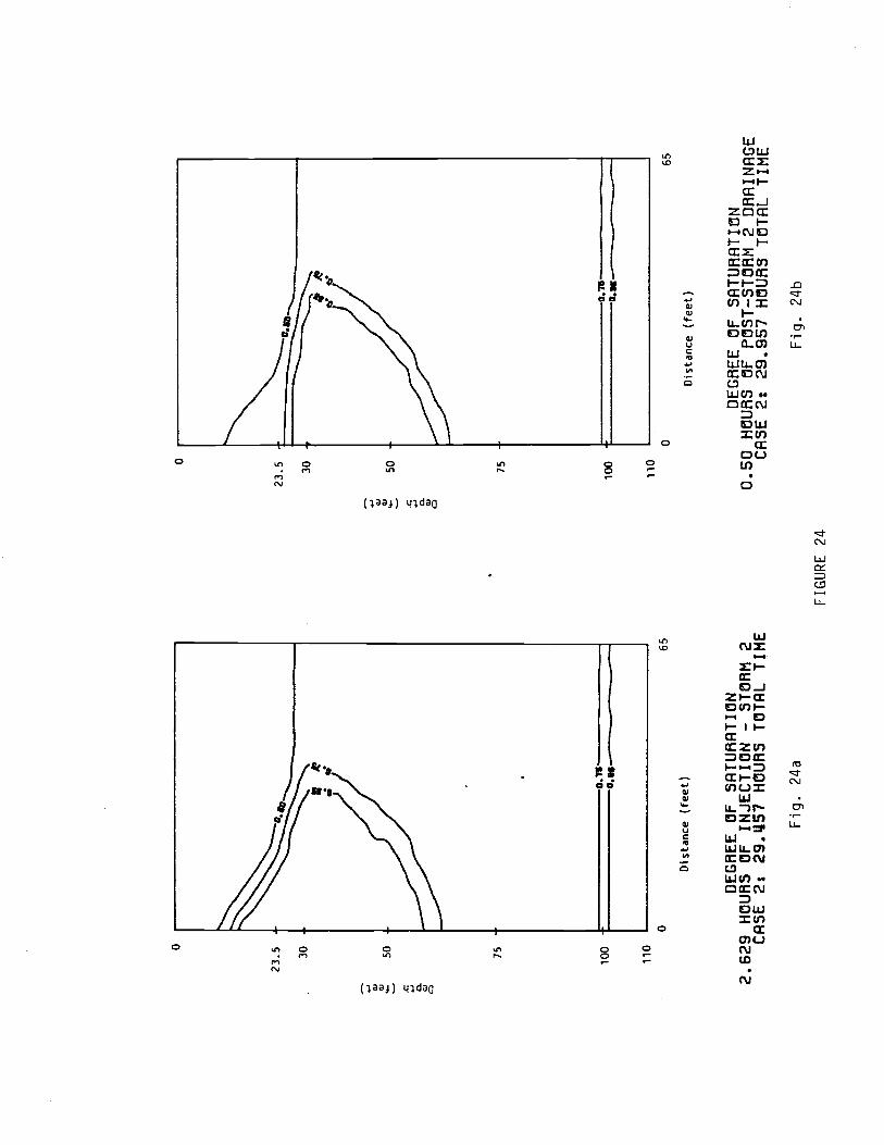
0

23.5

30 50

75

100

110

o..7

s

0

w

23.5 30

50

., Q.

CL

) 0

75

100

110

065

065

Distance (feet)

DEGREE OF SATURATION

2.629 HOURS OF INJECTION - STORM 2

CASE 2: 29.457 HOURS TOTAL TIME

Distance (feet)

DEGREE OF SATURATION

0.50 HOURS OF POST -STORM 2 DRAINAGE

CASE 2: 29.957 HOURS TOTAL TIME

Fig. 24a

Fig. 24b

FIGURE 24

0

23.5

1D

an

100

-

110

o

0.70

0.00

Distance (feet)

65

DEGREE OF SATURATION

9.00 HOURS OF POST -STORM 2 DRAINAGE

CASE 2: 38.4157 HOURS TOTAL TIME

Fig. 25a

FIGURE 25

0

100

110

0.70

0.00

o50

Distance (feet)

DEGREE OF SATURATION

20.00 HOURS OF POST -STORM 2 DRAINAGE

CASE 2: 149.457 HOURS TOTAL TIME

Fig. 25b

100

Q1

o

--'

O. S

O+

r-0

.70

r g a

-0.

700.

00

23.5

-23.5

30

50 75

100

110

050

Distance (feet)

DEGREE OF SATURATION

130.00 HOURS OF POST -STORM 2 DRAINAGE

CASE 2s 159.457 HOURS TOTAL TIME

Fig. 26a

100

30

Ql

50

Q CI

FIGURE 26

75

100

7

110

o50

Distance (feet)

DEGREE OF SATURATION

262.00 HOURS OF POST -STORM 2 DRAINAGE

CASE 2: 291.457 HOURS TOTAL TIME

Fig. 26b

100

0

23.5

30

50 75

100

110

0.60

0.70

o50

100

Distance (feet)

DEGREE OF SATURATION

286.00 HOURS OF POST -STORM 2 DRAINAGE

CASE 2: 315.157 HOURS TOTAL TIME

FIG

UR

E 2

7

0

23.5 30

a,

50

75

100.

0

21.0

00.0

\

1

05.0 00.0

l'71

3.a

00.0

00.0

00.0

310.

11

20.0

10.0

0

23.5

-t"

30

4,

YoO

d50

w á

75

-

100

100

-

110

o

Distance (feet)

50

HYDRAULIC HERD DISTRIBUTION (FEET)

0.50 HOURS OF INJECTION

CASE 2; STORM 1

110

10.0

50.0

20.0

20.0

11.0

10.0

050

Distance (feet)

HYDRAULIC HEAD DISTRIBUTION (FEET)

1.66 HOURS OF INJECTION

CASE 2; STORM 1

Fig. 28a

Fig: 28b

FIGURE 28

75 -

100

-

110

00.0

110.

0

OA

15.0

10.0

o50

23.5 30 50 75

SB

A

100

s-

110

00.0

110.

0

110.

0

15.0

10.0

o

Distance (feet)

Dis

tanc

e (f

eet)

HYDRAULIC HEAD DISTRIBUTION (FEET)

2.827 HOURS OF INJECTION - 5000 CU. FT.

CASE 2; STORM

1

50

HYDRAULIC HEAD DISTRIBUTION (FEET)

2.629 HOURS OF INJECTION: STORM 2

29.457 HOURS TOTAL TIME

Fig. 29a

Fig. 29b

FIGURE 29

0

75

-

100

-

110

0

0.7s

0.95

Distance (feet)

50

DEGREE OF SATURATION

0.50 HOURS OF INJECTION

CASE 3; STORM 1

Fig. 30a

0

23.5 30 -

0.50

75

100

-

110

0

0.75

0.96

Distance (feet)

50

DEGREE OF SATURATION

1.166 HOURS OF INJECTION

CASE 3; STORM 1

0

23.5

30

50

0.50

75

-

100

-

110

0

0.71

0.96

Distance (feet)

DEGREE OF SATURATION

2.00 HOURS OF INJECTION

CASE 3; STORM 1

Fig. 30b

Fig. 30c

FIGURE 30

0

23.5

-

30

-

50 -

75

-

110

0.60

0.78

o50

50

75

bO

61 q

DO

0.80

100

0.95

110

o

Distance (feet)

Distance (feet)

DEGREE OF SATURATION

2.75 HOURS OF INJECTION -

5000 CU. FT.

CASE 3: STORM 1

Fig. 31a

'60

DEGREE OF SATURATION

0.50 HOURS OF POST -STORM 1 DRAINAGE

CASE 3: 3.25 HOURS TOTAL TIME

Fig. 31b

FIGURE 31

23.5

30

100

110

rw

o

Distance (feet)

60

DEGREE OF SATURATION

2.75 HOURS OF POST -STORM 1 DRAINAGE

CASE 3: 5.50 HOURS TOTAL TIME

Fig. 31c

0

23.5 30

-

100

-

110

0

Distance (feet)

60

DEGREE OF SATURATION

6.25 HOURS OF POST -STORM 1 DRAINAGE

CASE 3: 9.00 HOURS TOTAL TIME

Fig. 32a

0

23.5

30

75

100

110

0.60

-.-...

4) 0.

800.

96

060

0

23.5

30

50

a t N a ó

75

100

-

110

0

0.80

0.9s

Distance (feet)

Distance (feet)

60

DEGREE OF SATURATION

DEGREE OF SATURATION

14.25 HOURS OF POST -STORM

1 DRAINAGE

24.00 HOURS OF POST -STORM 1 DRAINAGE

CASE 3:

17.00 HOURS TOTAL TIME

CASE 3: 26.75 HOURS TOTAL TIME

Fig. 32b

Fig. 32c

FIGURE 32

o

23.5 30 50 75

IMO

111.

0

-,ë.

01-

.....-

70.0

( l

0.0

i 44

116.

0

w'.Q

w.o

IMO

1110

.0

I0.0

MO

10.0

0

75

-

100

-100

-

110

o

Distance (feet)

50

HYDRAULIC HEAD DISTRIBUTION (FEET)

2.75 HOURS OF INJECTION - 5000 CU. FT.

CASE 3; STORM 1

110

00.0

10.0

10.0

p0.0

1.11

.0

050

Distance (feet)

HYDRAULIC HEAD DISTRIBUTION (FEET)

0.500 HOURS OF INJECTION

CASE 3; STORM 1

Fig. 33a

Fig. 33b

FIGURE 33