Jump Starting GARCH:

Pricing Options with Jumps in Returns and Volatilities

J. Duan ∗ P. Ritchken † Z. Sun ‡

November 30, 2007

∗Risk Management Institute and Department of Finance, National University of Singapore and Rotman School

of Management, University of Toronto. Email: bizdjc@nus.edu.sg.†Weatherhead School of Management, Case Western Reserve University, Cleveland, Ohio, 44106. Email:

peter.ritchken@case.edu.‡Fifth Third Asset Management,Cleveland, Ohio, 44114. Email: zhiqiang.sun@53.com.

Jump Starting GARCH:

Pricing and Hedging Options with Jumps in Returns and Volatilities

ABSTRACT

This paper considers the pricing of options when there are jumps in the pricing kernel andcorrelated jumps in asset returns and volatilities. Our model nests Duan’s GARCH optionmodels where conditional returns are constrained to being normal, as well as extends Merton’sjump-diffusion model by allowing return volatility to exhibit GARCH-like behavior. Empiricalanalysis on the S&P 500 index returns reveals that the incorporation of jumps in returns andvolatilities improves significantly the performance of the GARCH model in capturing the ob-served time series of the S&P 500 index returns. Moreover, the corresponding GARCH optionpricing model with the jump component delivers a better performance on pricing the S&P 500index options.

(GARCH, options, stochastic volatility, jumps)

In this paper we introduce a new family of GARCH models driven by compound Poissoninnovations and derive the corresponding option pricing theory. Because the compound Poissoninnovations are analogous to the increments in a continuous-time compound Poisson process, werefer to this new class as the GARCH-Jump model. These discrete-time processes are of interestsince the conditional returns of the underlying asset allow levels of skewness and kurtosis tobe matched to the data and option prices can readily be priced in a way to reflect changingvolatility and jumps in both returns and volatilities. This GARCH-Jump option pricing modelis a natural generalization of the typical GARCH option pricing models with normal innovations,a pricing approach originated in Duan (1995). We empirically test the model, and show thatit fits the return data better than the traditional GARCH model with normal innovations andoutperforms the inverse Gaussian GARCH model recently proposed by Christoffersen, Hestonand Jacobs (2006) (CHJ). Moreover, our model is better in removing more of the biases in optionprices.

Just as the binomial model serves as a discrete-time approximation for many underlyingdiffusion processes, the class of GARCH-Jump models can serve as discrete-time approxima-tions for an array of continuous-time jump diffusion models. As shown in Duan, Ritchkenand Sun (2006), a variety of continuous-time limiting models can in fact be derived using ourGARCH-Jump processes; for example, (1) when the GARCH feature is disabled but jumps al-lowed, the limiting model nests the jump-diffusion model of Merton (1976), (2) when jumps aresuppressed, the limiting model can be made to converge to continuous-time stochastic volatil-ity models, including Heston (1993), Hull and White (1987) and Scott (1987), among others,and (3) when jumps are permitted, the limiting models contain jumps and diffusive elements inboth returns and volatilities, along the lines of Eraker, Johannes and Polson (2003) and Duffie,Singleton and Pan (1999).

Furthermore, just as the appropriately defined binomial model provides a useful mechanismfor pricing American style options under the geometric Brownian motion assumption, our appro-priately defined risk neutralized discrete-time GARCH models provide a mechanism for pricingoptions when returns and/or volatilities experience random jumps. The option theoretical re-sults developed in this paper has in fact been utilized by Duan, Ritchken and Sun (2006) toderive the limiting option pricing models.

This paper contributes to the literature in three aspects. First, we propose a new class ofGARCH models based on compound Poisson innovations and establish the discrete-time optionpricing theory which allows us to price derivatives when the underlying asset’s innovations maybe far from normal and when volatility is stochastic. This is important because our approachoffers a unique GARCH option model with non-normal innovations that can be naturally linkedto stochastic volatility model with jumps.1 Second, we conduct an empirical analysis to demon-

1We know of three alternative ways of introducing non-normal innovations into the GARCH option pricing

1

strate the importance of incorporating jumps in returns and volatilities so as to better capturekurtosis and skewness in the time series return dynamics. Third, we employ a more compre-hensive approach to estimating parameters and comparing the performance of different optionmodels, that incorporates both the time series of asset returns as well as the cross section ofoption prices.

Why is it important to incorporate jumps in volatility? Empirical research has shown thatmodels which describe returns by a jump-diffusion process with volatility being characterized bya correlated diffusive stochastic process are incapable of capturing empirical features of equityindex returns or option prices. For example, both Bates (2000) and Pan (2002) argue forvolatility-jump models because implied volatilities move too abruptly for a diffusion.2 Whilejumps in the return process can explain large daily shocks, these return shocks are highlytransient and have no lasting effect on future returns. At the same time, with volatility beingdiffusive, changes occur gradually and with high persistence. These models are unlikely togenerate clustering of large returns associated with temporarily high levels of volatility, a featurethat is displayed by the data. Both of the above authors recommended considering models withjumps in volatility. Eraker, Johannes and Polson (2003) examined the jump in volatility modelsproposed by Duffie, Singleton and Pan (1999), and showed that the addition of jumps in volatilityprovide a significant improvement to explaining the returns data on the S&P 500 and Nasdaq 100index returns. In contrast, Eraker (2004) estimated parameters using the time series of returnstogether with the panel of option data, using methodology similar to Chernov and Ghysels (2000)and Pan (2002). He confirmed that the time series of returns was better described with a jumpin volatility. Surprisingly, however, the model did not provide significantly better fits to optionprices beyond the basic stochastic volatility model.

The GARCH model has been extensively used in studying return time series. In recent years,there has been an increasing use of the GARCH option pricing model to empirically examine itspricing performance. Heynen, Kemna and Vorst (1994), Duan (1996), Hardle and Hafner (2000),Heston and Nandi (2000), Duan and Zhang (2001), Lehar, Scheicher and Schittenkopf (2002),Lehnert (2003), Stentoft (2005) and Hsieh and Ritchken (2005), are some examples. Christof-fersen and Jacobs (2004) examined a set of GARCH option models using the more general

model. Duan (1999,2002) developed two versions of the GARCH option model allowing for conditional skewness

and kurtosis via a normal transformation technique and the entropy principle, respectively. Christoffersen, Heston,

and Jacobs (2006) developed a GARCH option pricing model using inverse Gaussian innovations.2Stochastic volatility option models have been considered by Hull and White (1987), Heston (1993),

Nandi (1998), Scott (1987), among others. Bakshi, Cao and Chen (1997) provided empirical tests of alterna-

tive option models, none of which contain jumps in volatility. Naik (1993) considered a regime switching model

where volatility can jump. For additional regime switching models, see Duan, Popova and Ritchken (2002). More

recently Bakshi and Cao (2003) provided empirical support for some stochastic volatility models with jumps in

returns and volatility. For alternative models see Alexander (2004), Brigo and Mercurio (2002), Brigo, Mercurio

and Rapisarda (2004), Carr and Wu (2003), and Madan, Carr and Chang (1998).

2

GARCH specification given in Ding, Granger and Engle (1993) and Hentschel (1995). Theyconcluded that while analysis of the return time series alone is in favor of more complex models,the option data suggest that the more parsimonious models with simple volatility clustering andleverage effects tend to have better performance. The GARCH option pricing models consideredin Christoffersen and Jacobs (2004) all have conditionally normal innovations. Our study us-ing the GARCH-Jump option pricing model thus adds to the empirical GARCH option pricingliterature.

Our empirical analysis focuses on a nested set of models that contain interesting special cases.At one extreme, we consider models where in the limit volatility does not jump, but returnscan jump. A Merton-like model is considered, where jump risk is not priced, and a generalizedversion of that model is also considered where jump risk is priced. At the other extreme weconsider models that contain no jumps but allows volatility to be time varying. Finally, weconsider models where jump and diffusive risks are priced and whose continuous-time limitscontain jumps in both returns and volatilities.

The paper proceeds as follows. In section 1 we provide the basic setup for the pricingkernel and the dynamics of the underlying asset. We also identify the risk neutral measure, andestablish our nested models which represent interesting special cases. In section 2 we discusstime series estimation and option pricing issues in the discrete-time GARCH-Jump framework.In section 3 we examine our nested GARCH-Jump models and present empirical evidence fromtime series of the S&P 500 index. In section 4 we employ an estimation method that combinestime series data with cross sectional data on option prices. We investigate the in-sample fitsof our nested models and compare them with the inverse Gaussian GARCH option model byChristoffersen, Heston and Jacobs (2006) that also employs non-normal innovations. Finally, weinvestigate how the option pricing models perform when the analysis is conducted using datain the out-of-sample period of up to 5 years after the model parameters have been estimated.Section 5 concludes.

1 The Basic Setup

We consider a discrete-time economy for a period of [0, T ] where uncertainty is defined ona complete filtered probability space (Ω,F , P) with filtration (Ft; t ∈ 0, 1, · · · , T) where F0

contains all P-null sets in F .

Let mt be the marginal utility of consumption at date t. For pricing to proceed, the jointdynamics of the asset price, and the pricing kernel, mt

mt−1, needs to be specified. We have

St−1 = EP[St

mt

mt−1

∣∣∣∣Ft−1

](1)

3

where St is the total payout, consisting of price and dividends. The expectation is taken underthe data generating measure, P, conditional on the information up to date t− 1.

We assume that the dynamics of this pricing kernel, mt/mt−1, is given by:

mt

mt−1= eat+bJt (2)

where at is the conditional mean growth rate of the pricing kernel and b is a scaling parameterto adjust the volatility of the pricing kernel; and Jt is a standard normal random variable plusa Poisson random sum of normally distributed variables. That is,

Jt = X(0)t +

Nt∑

j=1

X(j)t (3)

where

X(0)t ∼ N(0, 1)

X(j)t ∼ N(µ, γ2) for j = 1, 2, · · · ,

and Nt is distributed as a Poisson random variable with parameter λt, which may be stochasticbut is known at time t− 1 (i.e., Ft−1-measurable).3 The random variables X

(j)t are independent

for j = 0, 1, 2, · · · and t = 1, 2, · · · , T . Hence:

EP [Jt|Ft−1] = λtµ

V arP [Jt|Ft−1] = 1 + λt(µ2 + γ2).

Let rt denote the single period (from t− 1 to t) continuously compounded risk-free interestrate. Equilibrium implies that

EP[

mt

mt−1

∣∣∣∣Ft−1

]= e−rt (4)

Substituting for the dynamics of the pricing kernel, we obtain the following expectation:

EP[

mt

mt−1|Ft−1

]= eat+b2/2+λt(κ−1), (5)

whereκ = eµ+b2γ2/2.

Combining equations (12) and (5), we have:

rt = −(at + b2/2 + λt(κ− 1)

). (6)

3Maheu and McCurdy (2004), building on a model by Bates and Craine (1999), offered one interesting speci-

fication for time-varying λt.

4

Notice that the pricing kernel has local variance,

V arP[ln

(mt

mt−1

)|Ft−1

]= b2

[1 + λt(µ2 + γ2)

], (7)

and is time-varying as long as the jump intensity is time-varying. For the special case whenκ = 1, or equivalently when µ = −bγ2/2, the effects of the jump in the pricing kernel playno role on the interest rate. For all other values, the jump process explicitly affects both theinterest rate and asset price.

The asset price, St, is assumed to follow the process:

St

St−1= eαt+

√htJt (8)

where Jt is a standard normal random variable plus a Poisson random sum of normal randomvariables; αt is part of the conditional mean return to be determined later in Proposition 1; andht is a local scaling variable with its precise definition given later. In particular:

Jt = X(0)t +

Nt∑

j=1

X(j)t (9)

where

X(0)t ∼ N(0, 1)

X(j)t ∼ N(µ, γ2) for j = 1, 2, · · ·

Furthermore, for t = 1, 2, · · · , T :

CorrP(X(i)t , X(j)

τ ) =

ρ if i = j and t = τ

0 otherwise,

and Nt is the same Poisson random variable as in the pricing kernel.

The Poisson random variable provides shocks in period t. Given that the number of shocksin a particular period is some nonnegative integer k, say, the logarithm of the pricing kernel forthat period consists of a draw from the sum of k +1 normal distributions, while the logarithmicreturn of the asset also consists of a draw from the sum of k + 1 correlated normal randomvariables. In either case, the first normal random variable is standardized to have mean 0 andvariance 1 because its location and scale have already been reflected in the model specification.

Since:

EP [Jt|Ft−1

]= λtµ

V arP [Jt|Ft−1

]= 1 + λt(µ2 + γ2),

5

the local variance of the logarithmic returns for date t, viewed from date t− 1 is

V arP[ln

(St

St−1

)|Ft−1

]= ht(1 + λtγ

2), (10)

whereγ2 = µ2 + γ2.

We shall refer to ht as the local scaling factor because it differs from local variance by a factor.In general, the local scaling factor ht can be any predictable process. For example, it coulddepend on all previous scaling factors and shocks. That is:

ht = F (ht−i, Jt−i; i = 1, 2, · · ·) (11)

Equilibrium implies that

EP[

mt

mt−1|Ft−1

]= e−rt (12)

EP[

mt

mt−1

St

St−1|Ft−1

]= 1 (13)

These conditions impose a specific form on αt. The dynamics of the asset price can be rewrittenas in the following proposition.

Proposition 1

Under measure P, the dynamics of the asset price can be expressed as:

St

St−1= eαt+

√htJt (14)

where

αt = rt − ht

2−

√htbρ + λtκ (1−Kt) (15)

ht = F (ht−i, Jt−i; i = 1, 2, · · ·) (16)

Kt = exp(√

ht(µ + bργγ) +12htγ

2)

. (17)

Proof: See Appendix

1.1 Pricing Derivatives

It is both customary and arguably more desirable to price derivative claims using a risk neutralframework. Towards that goal we assume date T to be the terminal date that we are consideringand define measure Q by

dQ = exp

(T∑

t=1

rt

)mT

m0dP. (18)

6

Lemma 1

(i) Q is a probability measure.

(ii) For any Ft measurable contingent claim Zt, its time-(t-1) price is

Zt−1 = EP(

Ztmt

mt−1|Ft−1

)= e−rtEQ (Zt|Ft−1) .

Proof: See Appendix.

Given a specification for the dynamics of the pricing kernel and the state variable, all theinformation that is necessary for pricing contingent claims is provided. While pricing of all claimscan proceed, the advantage of the Q measure is that pricing can proceed as if risk neutralityholds.

Proposition 2

Under measure Q, the dynamics of the asset price is distributionally equivalent to:

St

St−1= eαt+

√htJt (19)

where

αt = rt − ht

2+ λt (1−Kt) (20)

ht = F (ht−i, Jt−i + bρ; i = 1, 2, · · ·) (21)

Jt = X(0)t +

Nt∑

j=1

X(j)t (22)

X(0)t ∼ N(0, 1) for t = 1, 2, · · · , T

X(j)t ∼ N(µ + bργγ, γ2) for t = 1, 2, · · · , T and j = 1, 2, · · ·

X(j)t are independent for t = 1, 2, · · · , T and j = 0, 1, 2, · · ·

Nt has a Poisson distribution with parameter λt ≡ λtκ and Kt has been defined in Proposition

1.

Proof: See Appendix

Under measure Q, the overall dynamics of the asset price is similar in form to the dynamicsunder the data generating measure, P. In particular, the logarithmic return is still a randomPoisson sum of normal random variables. However, under measure Q, the mean of each of thenormal random variables is shifted. Similarly, the random variable, Nt, distributed as a Poissonrandom variable under measure P, is still Poisson under measure Q but with a shifted parameter.

Notice that each normal random variable has the same variance under both measures. How-ever, the local variance of the innovation under measure Q is not equal to the local variance

7

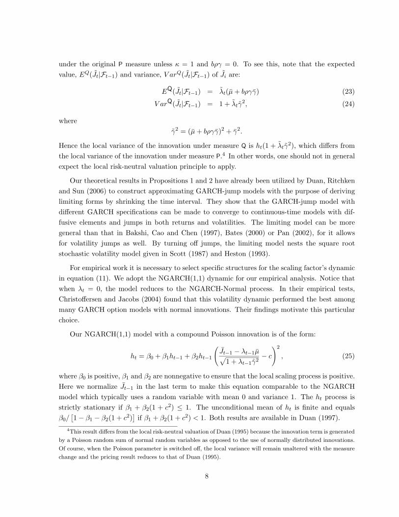
under the original P measure unless κ = 1 and bργ = 0. To see this, note that the expectedvalue, EQ(Jt|Ft−1) and variance, V arQ(Jt|Ft−1) of Ji are:

EQ(Jt|Ft−1) = λt(µ + bργγ) (23)

V arQ(Jt|Ft−1) = 1 + λtγ2, (24)

whereγ2 = (µ + bργγ)2 + γ2.

Hence the local variance of the innovation under measure Q is ht(1 + λtγ2), which differs from

the local variance of the innovation under measure P.4 In other words, one should not in generalexpect the local risk-neutral valuation principle to apply.

Our theoretical results in Propositions 1 and 2 have already been utilized by Duan, Ritchkenand Sun (2006) to construct approximating GARCH-jump models with the purpose of derivinglimiting forms by shrinking the time interval. They show that the GARCH-jump model withdifferent GARCH specifications can be made to converge to continuous-time models with dif-fusive elements and jumps in both returns and volatilities. The limiting model can be moregeneral than that in Bakshi, Cao and Chen (1997), Bates (2000) or Pan (2002), for it allowsfor volatility jumps as well. By turning off jumps, the limiting model nests the square rootstochastic volatility model given in Scott (1987) and Heston (1993).

For empirical work it is necessary to select specific structures for the scaling factor’s dynamicin equation (11). We adopt the NGARCH(1,1) dynamic for our empirical analysis. Notice thatwhen λt = 0, the model reduces to the NGARCH-Normal process. In their empirical tests,Christoffersen and Jacobs (2004) found that this volatility dynamic performed the best amongmany GARCH option models with normal innovations. Their findings motivate this particularchoice.

Our NGARCH(1,1) model with a compound Poisson innovation is of the form:

ht = β0 + β1ht−1 + β2ht−1

(Jt−1 − λt−1µ√

1 + λt−1γ2− c

)2

, (25)

where β0 is positive, β1 and β2 are nonnegative to ensure that the local scaling process is positive.Here we normalize Jt−1 in the last term to make this equation comparable to the NGARCHmodel which typically uses a random variable with mean 0 and variance 1. The ht process isstrictly stationary if β1 + β2(1 + c2) ≤ 1. The unconditional mean of ht is finite and equalsβ0/

[1− β1 − β2(1 + c2)

]if β1 + β2(1 + c2) < 1. Both results are available in Duan (1997).

4This result differs from the local risk-neutral valuation of Duan (1995) because the innovation term is generated

by a Poisson random sum of normal random variables as opposed to the use of normally distributed innovations.

Of course, when the Poisson parameter is switched off, the local variance will remain unaltered with the measure

change and the pricing result reduces to that of Duan (1995).

8

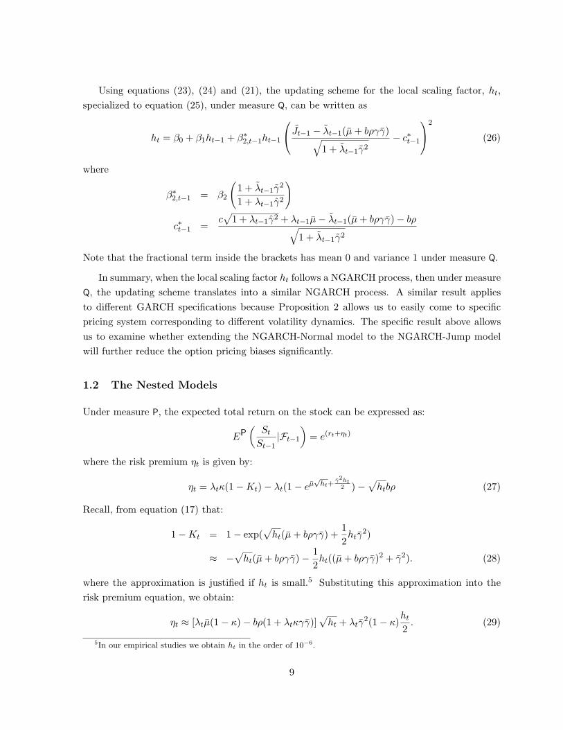
Using equations (23), (24) and (21), the updating scheme for the local scaling factor, ht,specialized to equation (25), under measure Q, can be written as

ht = β0 + β1ht−1 + β∗2,t−1ht−1

Jt−1 − λt−1(µ + bργγ)√

1 + λt−1γ2− c∗t−1

2

(26)

where

β∗2,t−1 = β2

(1 + λt−1γ

2

1 + λt−1γ2

)

c∗t−1 =c√

1 + λt−1γ2 + λt−1µ− λt−1(µ + bργγ)− bρ√1 + λt−1γ2

Note that the fractional term inside the brackets has mean 0 and variance 1 under measure Q.

In summary, when the local scaling factor ht follows a NGARCH process, then under measureQ, the updating scheme translates into a similar NGARCH process. A similar result appliesto different GARCH specifications because Proposition 2 allows us to easily come to specificpricing system corresponding to different volatility dynamics. The specific result above allowsus to examine whether extending the NGARCH-Normal model to the NGARCH-Jump modelwill further reduce the option pricing biases significantly.

1.2 The Nested Models

Under measure P, the expected total return on the stock can be expressed as:

EP(

St

St−1|Ft−1

)= e(rt+ηt)

where the risk premium ηt is given by:

ηt = λtκ(1−Kt)− λt(1− eµ√

ht+γ2ht

2 )−√

htbρ (27)

Recall, from equation (17) that:

1−Kt = 1− exp(√

ht(µ + bργγ) +12htγ

2)

≈ −√

ht(µ + bργγ)− 12ht((µ + bργγ)2 + γ2). (28)

where the approximation is justified if ht is small.5 Substituting this approximation into therisk premium equation, we obtain:

ηt ≈ [λtµ(1− κ)− bρ(1 + λtκγγ)]√

ht + λtγ2(1− κ)

ht

2. (29)

5In our empirical studies we obtain ht in the order of 10−6.

9

This form of the risk premia allows us to gain some insight into the pricing model.

(i) The Merton Model

First consider the case when κ = 1 and γ = 0. In this case, µ = 0 and there are no jumps inthe pricing kernel. The risk premium, ηt reduces to −bρ

√ht. That is, the risk premium does

not depend on jumps. With β1 = β2 = 0 in equation (25) the scaling factor remains constant.Since jump risk is diversifiable, the local scaling factor is constant, and innovations, conditionalon the number of jumps are normal, we refer to this model as the discrete-time Merton (1976)model, or Merton, for short.

(ii) The Generalized Merton Model

Second, consider the same model, but release κ and γ from 1 and 0. Naik and Lee (1990)extended Merton’s model to the case where jump risk is not diversifiable. In our model thisis accomplished by releasing κ from 1 and/or γ from 0. With κ 6= 1 and γ = 0 in the pricingkernel, the sensitivity of the risk premium to γ is very small. That is, the randomness aboutthe jump size adds minimally to the risk premium.

With κ = 1 and γ > 0, the risk premium is

ηt ≈ −bρ√

ht − bρλtγγ√

ht.

Here, the uncertainty of the jump size, as measured by γ, adds to the risk premium as does theintensity. This implies that jump risk is priced. With β1 = β2 = 0 in equation (25) the scalingfactor remains constant. We call this model the generalized Merton model.

(iii) The NGARCH-Normal Model

The third model we consider has no jumps, i.e., λt = 0, but with our scaling factor beingstochastic. In this case, innovations are normal random variables, and the risk premium is givenby ηt = −bρ

√ht. The system is referred to as the NGARCH-Normal model, or the NGARCH

model for short.

(iv) The Restricted NGARCH-Jump Model

The fourth model keeps κ = 1 and γ = 0 again, but the scaling factor is permitted to be stochasticand jumps in prices are allowed. In this model, jump risk is diversifiable, volatility is stochasticand innovations are non-normal. The model is referred to as the Restricted NGARCH-Jumpmodel, or restricted JGARCH for short.

(v) The NGARCH-Jump Model

The final model is the most general model where jump risk is priced, scaling factor is stochastic,jumps are present and innovations are not normal. The model is referred to as the NGARCH-Jump model, or JGARCH for short.

10

We will explore in the next section which of the models nested in our family can explain boththe time series of the S&P 500 index values and the cross sectional variation of option pricesover a broad array of strikes and maturities.

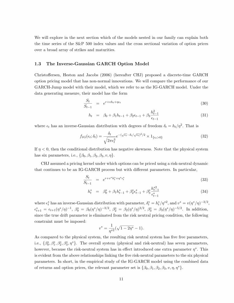
1.3 The Inverse-Gaussian GARCH Option Model

Christoffersen, Heston and Jacobs (2006) (hereafter CHJ) proposed a discrete-time GARCHoption pricing model that has non-normal innovations. We will compare the performance of ourGARCH-Jump model with their model, which we refer to as the IG-GARCH model. Under thedata generating measure, their model has the form

St

St−1= er+vht+ηεt (30)

ht = β0 + β1ht−1 + β2εt−1 + β3h2

t−1

εt−1(31)

where εt has an inverse-Gaussian distribution with degrees of freedom δt = ht/η2. That is

fIG(εt; δt) =δt√2πε3t

e−(√

εt−δt/√

εt)2/2 × 1εt>0 (32)

If η < 0, then the conditional distribution has negative skewness. Note that the physical systemhas six parameters, i.e., β0, β1, β2, β3, v, η.

CHJ assumed a pricing kernel under which options can be priced using a risk-neutral dynamicthat continues to be an IG-GARCH process but with different parameters. In particular,

St

St−1= er+v∗h∗t +η∗ε∗t (33)

h∗t = β∗0 + β1h∗t−1 + β∗2ε∗t−1 + β∗3

h∗2t−1

ε∗t−1

(34)

where ε∗t has an inverse-Gaussian distribution with parameter, δ∗t = h∗t /η∗2, and v∗ = v(η∗/η)−3/2,ε∗t+1 = εt+1(η∗/η)−1, β∗0 = β0(η∗/η)−3/2, β∗2 = β2(η∗/η)3/2, β∗3 = β3(η∗/η)−5/2. In addition,since the true drift parameter is eliminated from the risk neutral pricing condition, the followingconstraint must be imposed:

v∗ =1

η∗2(√

1− 2η∗ − 1).

As compared to the physical system, the resulting risk neutral system has five free parameters,i.e., β∗0 , β∗1 , β∗2 , β∗3 , η∗. The overall system (physical and risk-neutral) has seven parameters,however, because the risk-neutral system has in effect introduced one extra parameter η∗. Thisis evident from the above relationships linking the five risk-neutral parameters to the six physicalparameters. In short, in the empirical study of the IG-GARCH model using the combined dataof returns and option prices, the relevant parameter set is β0, β1, β2, β3, v, η, η∗.

11

2 Data

We examine the performance of the above models using time series data on the S&P 500 indexand dividends, as well as option price information on the S&P 500 index.

The S&P 500 index options are European options that exist with maturities in the nextsix calendar months, and also for the time periods corresponding to the expiration dates of thefutures. Our price data on the options, spans the time period from January 1996 to June 2005.The data comes from Ivy OptionMetrics database which is a comprehensive database coveringUS index and equity options markets. From this database we extract daily highest closing bidand lowest closing ask prices across all exchanges for each option contract on the S&P 500index. In addition we record the time to expiration, the strike price, and the closing price ofthe S&P 500 index. We only consider option contracts that have a time to expiration greaterthan 10 days and less than 120 days. We also exclude those option contracts that are so faraway from the money that there are liquidity concerns. In particular we exclude an option whenthe midpoint of the bid-ask price is below intrinsic value, when the vega of the option is below0.5, and when the implied volatility calculation fails to converge. We also record the interestrate information on each day, and the dividend yield that OptionMetrics uses to compute theBlack-Scholes implied volatilities.

The interest rates that are available from OptionMetrics correspond to the continuouslycompounded zero-rates derived from LIBOR rates and settlement prices of CME Eurodollarfutures. For any given option, the appropriate interest rate corresponds to the zero rate thathas maturity equal to the option’s expiration, and is obtained by interpolating between the twoclosest zero rates on the zero curve.

In order to price the options we need to adjust the index level according to the dividends paidout over the time to expiration. Harvey and Whaley (1992), and Bakshi, Cao and Chen (1997),used the actual cash dividend payments made during the life of the option to proxy for theexpected dividend payments. The present value of all the dividends was then subtracted fromthe reported index levels to obtain the contemporaneous adjusted index levels. This procedureassumes that the reported index level is not stale and reflects the actual price of the basket ofstocks representing the index when the option quotes were obtained. There are other methodsfor establishing the dividend adjusted index level. The first is to use the stock index futures priceto back out the implied dividend adjusted index level. This leads to one stock index adjustedvalue that is used for all option contracts with the same maturity. The second is to compute themid points of call and put options with the same strikes and then to use put-call parity to implyout the value of the underlying index. OptionMetrics uses a regression approach that exploitsput-call parity conditions repeatedly over a number of contracts and over a ten-day period toextract an implied dividend yield that they apply to all option contracts. We use their extracted

12

dividend yield in all our computations. For a discussion of different approaches see Jackwerthand Rubinstein (1996).

We extract option prices on a weekly basis, each Wednesday, over the 9.5-year period (Jan-uary 1996 to June 2005). For the underlying S&P 500 index we obtain the time series of dailyreturns going back to January 1970. We have 43, 377 option contracts that pass all the filters,with the number of contracts each year ranging from a low of 2,306 for the six month period in2005 to a high of 5,069 contracts in 2002.

We split up our data set into two, an “in-sample” period extending over the first 5 years,and an “out-of-sample” period covering the remaining 5 years.

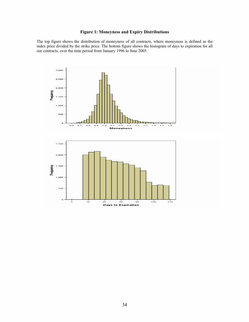
We define moneyness as the index price relative to the strike price. We construct histogramsof moneyness and days to expiration. The top graph of Figure 1 shows the distribution ofmoneyness over the in-sample period, and the bottom figure shows the distribution of expirationdates. The mode of the distribution is at the short maturities. Over 90% of maturities are within90 days. We construct buckets of maturities, defining bin 1 as those contracts that expire within30 days; bin 2, those that expire in the 31-60 day range; bin 3, those that expire in the 61-90day range and bin 4 are those contracts that have longer expiration dates.

Figure 1 Here

Table 1 shows the number of option contracts by moneyness and by maturity and the averageimplied volatilities for each of the moneyness-maturity bins. We see from the table that thelargest variation in volatilities across strike prices occurs for the shorter-term option contracts.

Table 1 Here

The top graph in Figure 2 plots the average monthly volatility smile by moneyness over theten-year time period for all contracts less than 30 days. The exact shape of the volatility smilefluctuates over time. From this figure we see that deep in-the-money calls generally have thelargest volatilities. The bottom graph in Figure 2 shows the time series behavior of at-the-moneyimplied volatilities over the ten-year period. As can be seen volatilities have fluctuated from10% to over 30%.

Figure 2 Here

13

3 Estimation of Models Using Time Series of Returns and/or

Option Prices

Our first set of experiments are concerned with using the time series return data on the S&P500 index alone to compare the performance of some of the models nested in the GARCH-Jumpfamily, and to contrast these models with the IG-GARCH model.

We apply the maximum-likelihood method on the time series of index returns to estimatethe model parameters. Our model parameter set is θ = β0, β1, β2, c, bρ, κ, γ, µ, γ, λ. DefineRt ≡ ln(St/St−1). The conditional probability density function for Rt is:

l (Rt|ht) =∞∑

i=0

λi

i!e−λf

(Rt − αt; µi(t), σ2

i (t))

(35)

where αt is given in Proposition 1; the NGARCH(1,1) local scaling factor, ht, is by equation(25); and f

(·; µi(t), σ2i (t)

)is the normal density function with mean µi(t) = iµ

√ht and variance

σ2i (t) = ht(1 + iγ2).6 The initial value of the local scaling factor is set according to

h1 = V/(1 + λγ2) (36)

where V is the sample variance of the asset return and as defined earlier, γ2 = µ2 + γ2.7

The log-likelihood function for the sample of asset prices is:

L(θ; S1, S2, · · · , ST ) =T∑

t=2

ln [l (Rt|ht)] . (37)

The maximum likelihood estimator for θ is the solution of maximizing the above log-likelihoodfunction. Given the asset price time series, St1≤t≤T , we can compute the log-likelihood func-tion recursively, and solve this optimization problem numerically.

In principle, the entire set of parameters can be identified by only using a return timeseries. In practice, however, two of them are hard to pin down empirically. To understand thisassertion, notice that conditional on αt the log-likelihood function is fully determined by µ, γ2,λ, and the parameters driving the variance updates – β0, β1, β2, and c. To fully characterizethe log-likelihood function, we of course need to know αt, which in turn requires knowledgeof three extra parameters, namely µ, γ and bρ. Recall from equation (28) that: 1 − Kt ≈−√ht(µ + bργγ)− 1

2ht((µ + bργγ)2 + γ2). Substituting this expression into equation (15) leads

6Conditioning on Nt = i, the variance of Jt is 1 + iγ2. Without conditioning, however, the variance becomes

1 + λγ2.7Note that V arP(Jt) = (1+λγ2). Thus, we have in essence removed the extra volatility arising from the jump

component in setting the initial value of the scaling factor process.

14

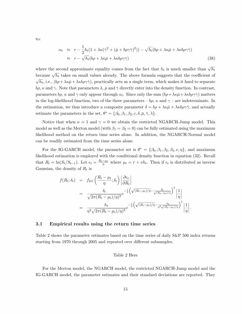
to:

αt ≈ r − 12ht(1 + λκ(γ2 + (µ + bργγ)2))−

√ht(bρ + λκµ + λκbργγ)

≈ r −√

ht(bρ + λκµ + λκbργγ) (38)

where the second approximate equality comes from the fact that ht is much smaller than√

ht

because√

ht takes on small values already. The above formula suggests that the coefficient of√ht, i.e., (bρ+λκµ+λκbργγ), practically acts as a single term, which makes it hard to separate

bρ, κ and γ. Note that parameters λ, µ and γ directly enter into the density function. In contrast,parameters bρ, κ and γ only appear through αt. Since only the sum (bρ+λκµ+λκbργγ) mattersin the log-likelihood function, two of the three parameters – bρ, κ and γ – are indeterminate. Inthe estimation, we thus introduce a composite parameter δ = bρ + λκµ + λκbργγ, and actuallyestimate the parameters in the set, θ∗ = β0, β1, β2, c, δ, µ, γ, λ.

Notice that when κ = 1 and γ = 0 we obtain the restricted NGARCH-Jump model. Thismodel as well as the Merton model (with β1 = β2 = 0) can be fully estimated using the maximumlikelihood method on the return time series alone. In addition, the NGARCH-Normal modelcan be readily estimated from the time series alone.

For the IG-GARCH model, the parameter set is θ∗ = β0, β1, β2, β3, v, η, and maximumlikelihood estimation is employed with the conditional density function in equation (32). Recallthat Rt = ln(St/St−1). Let εt = Rt−µt

η where µt = r + vht. Then if εt is distributed as inverseGaussian, the density of Rt is

f(Rt; δt) = fIG

(Rt − µt

η; δt

) ∣∣∣∣∂εt

∂Rt

∣∣∣∣

=δt√

2π(Rt − µt)/η)3e− 1

2

(√(Rt−µt)/η− δt√

(Rt−µt)/η

)2 ∣∣∣∣1η

∣∣∣∣

=ht

η2√

2π(Rt − µt)/η)3e− 1

2

(√(Rt−µt)/η− ht

η2√

(Rt−µt)/η

)2 ∣∣∣∣1η

∣∣∣∣ .

3.1 Empirical results using the return time series

Table 2 shows the parameter estimates based on the time series of daily S&P 500 index returnsstarting from 1970 through 2005 and repeated over different subsamples.

Table 2 Here

For the Merton model, the NGARCH model, the restricted NGARCH-Jump model and theIG-GARCH model, the parameter estimates and their standard deviations are reported. They

15

are followed by the maximum log-likelihood value and the Akaike Information Criterion (AIC)which measures model performance by accounting for goodness of fit and parsimony. A smallerAIC indicates a better performance.

For the two models (Merton and NGARCH-Normal) nested in the restricted NGARCH-Jump model, one can use the likelihood ratio test to evaluate whether there is any incrementalvalue in adding complexity to the Merton model. Under the null hypothesis that the morecomplex model does not add significantly, two times the difference in the log-likelihood valuesshould distribute as a chi-square distribution with the degrees of freedom equal to the differencein the numbers of parameters of the two models.

The likelihood ratio test based on Table 2 indicates that, at the 1% level, the restrictedNGARCH-Jump model is a significant improvement over the Merton model. This suggests thatreturn data exhibits the GARCH feature. Further, the likelihood ratio test reveals that the effectof adding jumps to the NGARCH model leads to significant improvements. Specifically, Table2 reveals that λ is significantly different from 0, indicating that the incorporation of jumps issignificant and the conditional distribution exhibits skewed and heavy-tailed behavior. For therestricted NGARCH-Jump model, the non-linear term c, capturing the so called leverage effect,continues to be significant after adding jumps to the NGARCH model. In addition, the resultsare similar for the two sub-samples. The results based on the AIC criterion also lead to thesame conclusion. Taken together, the restricted NGARCH-Jump model is clearly the dominantmodel in this nested class.

Eraker, Johannes and Polson (2003) find that jumps are infrequent events, occurring onaverage about twice every three years, tend to be negative, and are very large relative to normalday to day movements. In contrast, our average “jump” frequency is over two a day. In ourmodel the jumps add conditional skewness and kurtosis to the daily innovations, rather thanproviding large shocks. Indeed, the mean and standard deviation of our jump size variable is notparticularly large compared to the standard normal innovation. By mixing a random number ofnormal distributions, the conditional distribution displays higher kurtosis. In our case Jt consistsof one standard normal random variable together with a Poisson random sum of independentnormal random variables with mean µ and variance γ2.

The results in Table 2 reveals that the performance of the IG-GARCH model according to theAIC criterion is markedly worse than either the NGARCH-Normal or restricted NGARCH-Jumpmodel in the whole sample as well as in two sub-samples. The fact that it is even worse than theNGARCH-Normal model is particularly worth noting. Although the IG-GARCH model allowsfor non-normal conditional innovations, it relies on a GARCH specification that is less compatiblewith the data than is the NGARCH model. As a result, the NGARCH model restricted to normalconditional innovations can still outperform the IG-GARCH model in terms of the log-likelihoodvalue even before accounting for the compensation factor due to fewer model parameters.

16

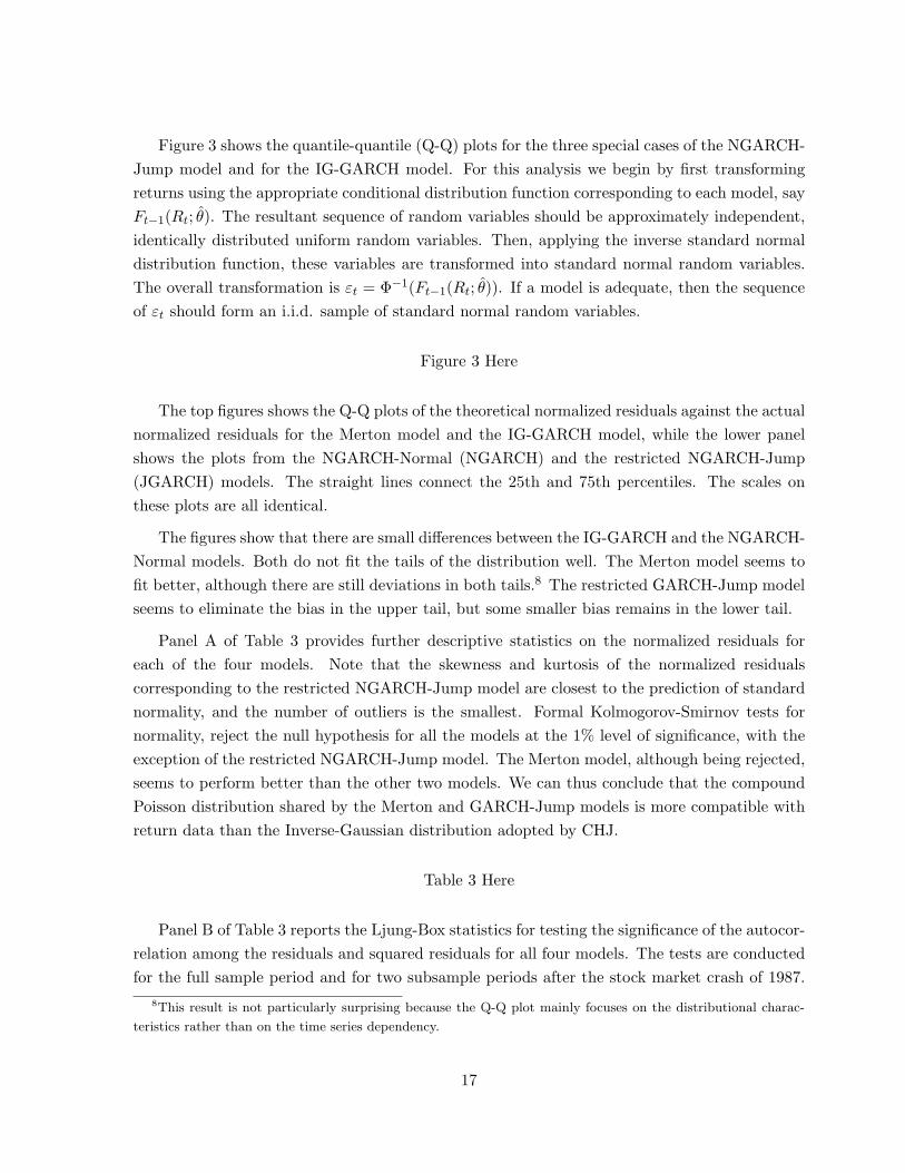
Figure 3 shows the quantile-quantile (Q-Q) plots for the three special cases of the NGARCH-Jump model and for the IG-GARCH model. For this analysis we begin by first transformingreturns using the appropriate conditional distribution function corresponding to each model, sayFt−1(Rt; θ). The resultant sequence of random variables should be approximately independent,identically distributed uniform random variables. Then, applying the inverse standard normaldistribution function, these variables are transformed into standard normal random variables.The overall transformation is εt = Φ−1(Ft−1(Rt; θ)). If a model is adequate, then the sequenceof εt should form an i.i.d. sample of standard normal random variables.

Figure 3 Here

The top figures shows the Q-Q plots of the theoretical normalized residuals against the actualnormalized residuals for the Merton model and the IG-GARCH model, while the lower panelshows the plots from the NGARCH-Normal (NGARCH) and the restricted NGARCH-Jump(JGARCH) models. The straight lines connect the 25th and 75th percentiles. The scales onthese plots are all identical.

The figures show that there are small differences between the IG-GARCH and the NGARCH-Normal models. Both do not fit the tails of the distribution well. The Merton model seems tofit better, although there are still deviations in both tails.8 The restricted GARCH-Jump modelseems to eliminate the bias in the upper tail, but some smaller bias remains in the lower tail.

Panel A of Table 3 provides further descriptive statistics on the normalized residuals foreach of the four models. Note that the skewness and kurtosis of the normalized residualscorresponding to the restricted NGARCH-Jump model are closest to the prediction of standardnormality, and the number of outliers is the smallest. Formal Kolmogorov-Smirnov tests fornormality, reject the null hypothesis for all the models at the 1% level of significance, with theexception of the restricted NGARCH-Jump model. The Merton model, although being rejected,seems to perform better than the other two models. We can thus conclude that the compoundPoisson distribution shared by the Merton and GARCH-Jump models is more compatible withreturn data than the Inverse-Gaussian distribution adopted by CHJ.

Table 3 Here

Panel B of Table 3 reports the Ljung-Box statistics for testing the significance of the autocor-relation among the residuals and squared residuals for all four models. The tests are conductedfor the full sample period and for two subsample periods after the stock market crash of 1987.

8This result is not particularly surprising because the Q-Q plot mainly focuses on the distributional charac-

teristics rather than on the time series dependency.

17

The autocorrelation of residuals produced by all models is significant at the 5% level. Thissignificance can be traced back to the very high autocorrelation in the raw returns that existedin the early data period from 1970 to 1987, likely due to non-synchronous trading among theS&P 500 component stocks in this earlier period. In the two subperiods after 1987, all modelsproduced residuals that were not significantly autocorrelated.

As can be seen from the table, the autocorrelation among the squared residuals produced bythe Merton model is significant for the entire sample as well as for each of the two subsamples.The two NGARCH models were effective in removing autocorrelation in the squared residuals.In contrast, the IG-GARCH model still yields significantly autocorrelated squared residuals forthe whole sample, indicating that the IG-GARCH volatility specification is less compatible withthe data.

3.2 Empirical results using time series of returns and option prices

There are several ways in which option pricing models can be evaluated.9 First, one can estimateall model parameters with the underlying asset price series. The estimated parameters can thenbe used in the option pricing system (under measure Q) to price all options. This implementationcan be likened to estimating historical volatilities from the return data and then evaluating theBlack-Scholes formula based on these estimates. This approach is obviously quite demanding onan option pricing model because option data have not been used in the parameter estimation.For the NGARCH-Jump model, as discussed earlier, there is also an econometric complexityassociated with only using the return data. Specifically, for this model, some parameters (i.e.,bρ, κ and γ) are difficult to identify from the return time series alone. This approach is thus notpractically advisable.

The second way of implementation uses option data in estimation. The underlying returnseries is used to update the local volatility but it does not directly enter into the likelihoodfunction in parameter estimation. This approach is in a way like running a nonlinear regressionby treating the underlying asset price as an exogenous variable. In the Black-Scholes framework,this is analogous to obtaining just one implied volatility by pooling the information from manyoptions together. For the GARCH option pricing model, one can obtain the time series ofvolatilities, corresponding to a set of parameters and conditional on stock price moves, andthen periodically price some panels of option contracts. The optimization criterion typicallyfocuses on minimizing sums of squared option pricing errors. This approach clearly overlooksthe information embedded in the underlying return time series because such series also providesuseful information concerning the basic premise of an option pricing model; that is, the assumeddynamic for the underlying asset price. The implementation of the GARCH option pricing model

9For an excellent review of empirical option pricing see Bates (2003).

18

adopted by Heston and Nandi (2000), Christoffersen and Jacobs (2004), Hsieh and Ritchken(2005) all fall in this category.

The third and better way of implementing an option pricing model is to combine the optionand underlying asset prices over the sample period to conduct a joint estimation of the model.Thus, both option and underlying asset prices directly enter into the joint likelihood functiondescribing the overall system. For ease of exposition, we will refer to this method as the panelestimation approach which has been adopted in our empirical analysis.

The panel estimation approach can be implemented in many different ways. The part con-cerning the underlying return time series is rather straightforward because it follows directlyfrom our GARCH-Jump specification. For option prices, one does have a choice, namely usingthe prices directly, or transforming them to the Black-Scholes implied volatilities. In essence,the choice amounts to opting for a particular specification for the cross-sectional error struc-ture. Since option prices naturally vary according to their strike prices and maturities, impliedvolatilities offer a cross-sectional data standardization that is intuitively appealing and conve-niently tied-to common industry practice of quoting implied volatilities in referring to optioncontracts. In short, our specific panel estimation approach take a vector of observations at atime point whose first entry is always the underlying asset price and remaining entries are theimplied volatilities of options included in our sample. Note that the dimension of this datavector depends on the availability of options at a particular time point, as well as our decisionas to which options to include. We derive the joint likelihood function for such kind of datavectors over the sample period and use the joint likelihood function to conduct the maximumlikelihood parameter estimation.

Denote the data vector at time by Dt(mt); that is, Dt(mt) = (St, IVt,1, · · · , IVt,mt)′ wheremt is the number of options at time t being included and IVt,j is the Black-Scholes impliedvolatility of the j-th option at time t. The joint log-likelihood function thus becomes

L(θ, ω; D1(m1), · · · , DT (mT ))

=T∑

t=2

ln [l (Rt|ht)]−(

ln(2π)2

+ ln(ω)) T∑

t=1

mt − 12ω2

T∑

t=1

mt∑

j=1

(IVt,j − ˆIV t,j(θ)

)2

where the expression for l (Rt|ht) is available in equation (35); and ˆIV t,j(θ) is the Black-Scholesimplied volatility computed from the GARCH option price of the j-th option at time t evaluatedat parameter θ. The first term on the right-hand side is the log-likelihood associated with theunderlying stock price time series. The summation begins from t = 2 because the first stock priceis only used to anchor the conditional distribution for the second stock price. The second andthird terms on the right-hand side is the log-likelihood function of the option data conditionalon the underlying stock price series. We have assumed that the errors in terms of impliedvolatilities share the same magnitude and are independent across options and over time. The

19

error distribution is assumed to be normal with a standard deviation of ω. Needless to say, thisrestriction can be relaxed, such as allowing for time and/or cross-sectional dependency, at theexpense of introducing more parameters.

For the NGARCH-Jump model, the combined data of asset and option prices can be usedto identify the full parameter set governing this option pricing model. In this case, θ =β0, β1, β2, c, bρ, κ, γ, µ, γ, λ. The whole set of parameters to be estimated is thus composedof θ and ω. In the case of the IG-GARCH model, the full parameter set governing this optionpricing model is θ = β0, β1, β2, β3, v, η, η∗. Again the whole set of parameter to be estimatedconsists of θ and ω.

We use the time series of daily returns up to the first Wednesday in January 1996 to updateour local scaling factor. Then, given the dividend adjusted index at that date, and using theterm structure of riskless rates at that date, we numerically compute the theoretical optionprices of selected call and put contracts for a given model. Since there are no simple analyticalexpressions for the NGARCH option pricing models, their prices are generated by Monte Carlosimulation. For a fair comparison, we also use the same stream of random numbers to generatethe prices for the IG-GARCH model. We use 5,000 sample paths to generate Monte Carlo optionprices. To improve the quality of Monte-Carlo prices, we apply the analytical pricing formulaon the last day of the contract because the analytical solution does exist for one-day optioncontracts. We then compute the implied volatilities using the Black Scholes model, and theresulting values are used in the log-likelihood function. We then use the daily returns to updatethe local volatility to the next time point on which the next set of option prices is available.The process is repeated and the individual log-likelihood is added to the overall log-likelihoodfunction. We continue this process for all days in the estimation period.

We split our option data into two – the “in-sample” period starting in 1996 and extendingthrough 2000 and the “out-of-sample” period with the remaining data. Our initial parameterestimates are taken from the return time series analysis that uses all information up to 1996.The likelihood function then consists of the time series component together with informationfrom options taken every fourth week up to the end of 2000. As a result we have used 60 panelsof cross sectional option vectors, together with the 5 years of daily return time series informationin the parameter estimation. The option contracts used in the optimization include all contractswith maturities between 10 and 90 days and moneyness within 5% of the index value.

Once the optimized parameter values are obtained, we use them and the daily time series ofthe S&P 500 index to compute the full time series of the local scaling factor over both the in- andout-of-sample periods. Then, for each Wednesday, given the index level and the updated scalingfactor, together with interest rate and dividend information, we can compute the theoreticalimplied volatilities and compare to their actual counterparts. We do this for each week in thein-sample period and for each week in the 5 years corresponding to the “out-of-sample” period.

20

Further, we compute prices for the longer maturity contracts (maturities that exceed 90 days)and moneyness factors that were never used in the optimization. The residuals obtained fromdifferent models then form the basis for our comparisons of the models. An option model isviewed positively if the in-sample fits are more precise and less biased, and if, conditional onfuture up-to-date index values, the “out-of-sample” price predictions are also more precise andless biased.

Before presenting the results, it should be noted that our objective is not to fit the volatilitysmile precisely at any one date. Were this curve fitting exercise the goal, we would merely chooseparameter sets each week that minimize the sum of squared errors (in implied volatilities) fordifferent models. By using 5 years of data to choose one set of parameters, our fits of impliedvolatilities at any week in the in-sample period will naturally be less precise than models obtainedby more frequent recalibrations. Further, in our “out-of-sample” period, we would expect theperformance of all models to deteriorate over time, especially when parameter estimates are notupdated, say after 5 years. However, our goal here is only to compare the relative performanceof these models under identical conditions. Any model that is successful in these tests can thenbe further scrutinized by evaluating its performance with more frequent parameter updates.

Table 4 reports the parameter estimates for the generalized Merton, the NGARCH-Normal,the IG-GARCH, and the NGARCH-Jump models, together with their log-likelihood values inthe in-sample setting. Note that in the case of the generalized Merton model, jump risk is allowedto be priced. In terms of NGARCH-Jump model, we no longer need to apply the restricted formbecause all parameters can be identified with the added information from option prices.

Table 4 Here

The likelihood ratio tests reveal that at the 1% level of significance, the NGARCH-Jumpmodel improves significantly over the NGARCH-Normal model, and is also superior to thegeneralized Merton model. These results echo the earlier findings based on the return timeseries only. In short, both the GARCH effect and jumps play critical roles in capturing datafeatures.

For comparing the non-nested models, we again resort to the AIC. The results in Table 4 showa clear dominance of the NGARCH-Jump model over the IG-GARCH model. The NGARCH-Normal also dominates the IG-GARCH model. Strikingly perhaps, the NGARCH-Normal modelcan dominate the IG-GARCH model based on the log-likelihood values even before factoring inits smaller set of parameters (6 vs. 8). The results from the combined data of returns and optionprices indicate that the restricted form of the volatility dynamic essential to the IG-GARCHmodel is at odds with the data. In summary, simply incorporating skewed and/or heavy-tailedinnovations into a GARCH model need not work well on return and/or option data. A suitable

21

volatility specification may be more important than the form of the conditional distribution forreturn innovations.

The two parameters, κ and γ, can be identified under the NGARCH-Jump model with thecombined data. Their individual parameter estimates, κ = 1.186 and γ = 0.41392, differ fromthe theoretical values of 1 and 0 predicted when the jump risk is not priced, but not statisticallysignificant. For the IG-GARCH model, the coefficient multiplying the inverse Gaussian innova-tion hardly changes from the physical measure to the risk-neutral measure (from η = 5.99×10−4

to η∗ = 5.92× 10−4).

Once the parameters are estimated, theoretical prices for all option contracts, includingthose with strike prices more than 5% away from the money, and with maturities exceeding 90days are computed on each Wednesday, and their Black-Scholes implied volatilities established.The residuals are then established as the difference between theoretical and observed impliedvolatilities. Figure 4 shows a box and whiskers plot of these residuals by moneyness for each ofthe four models. Thirteen moneyness buckets were established with mean moneyness in eachbucket ranging from 0.85 to 1.07, with the at-the-money contracts being in group 9. The figureclearly reveals that the generalized Merton model is incapable of removing significant biasesalong the moneyness dimension. At-the-money contracts are priced with little bias, but deepout-the-money contracts are overpriced and deep in-the-money contracts are underpriced.

Figure 4 Here

The plots of the NGARCH-Normal and IG-GARCH models are fairly similar to that of thegeneralized Merton model, in that the patterns of skewness are the same although of a muchsmaller magnitude. The NGARCH-Jump model has the least bias of all the models and clearlyproduces small biases for deep in-the-money contracts.

Figure 5 shows the box and whiskers plots of the residuals by maturity buckets for each ofthe four models also using all contracts in the in-sample period. For each maturity bucket, thereare four box and whiskers plots representing from left to right the generalized Merton model, theNGARCH-Normal model, the IG-GARCH model and the NGARCH-Jump model, respectively.

Figure 5 Here

This figure shows large biases and large interquartile ranges for the generalized Mertonmodel. For short-maturity contracts the NGARCH-Jump model displays some bias. For theother maturities the bias is slight and the interquartile ranges are smaller than the other models.Except for the generalized Merton model, the models seem to work roughly the same viewedfrom the maturity dimension.

22

Table 5 shows the proportion of times the NGARCH-Jump model produces a smaller abso-lute error than the other models. These comparisons are conducted over both moneyness andmaturity buckets. For ease of displaying the results the moneyness categories are reduced to 5,with group 3 being at-the-money. Nonparametric tests of the null hypothesis that the proportionof wins is 50% against the alternative that the proportion is larger than 50% are conducted.The bold-faced numbers indicate those moneyness-maturity combinations where the reportedproportion is significantly different, at the 1% level, from 50%. We also report the results ofpairwise comparisons between the NGARCH-Normal and IG-GARCH models and between thesemodels and the generalized Merton model. The left column reports the results for the in-sampleperiod and the right side reports the results for the out-of-sample period.

Table 5 Here

The results show how poorly the Merton model performs against all other models. It alsoshows that the overall performance the NGARCH-Normal model is comparable to that of theIG-GARCH model in the in-sample test but it dominates in the out-of-sample analysis. Overallthe NGARCH-Jump model outperforms all others in both “in-sample” and “out-of-sample”tests.

Our last set of analyses in this section deals with “out-of-sample” performance using the lastfive years of data. Figure 6 compares the time series of at-the-money volatilities averaged overa month with their theoretical counterparts for each of the four models. For the first 60 monthsthese are “in-sample”’ values. After that, the implied volatilities are “out-of-sample”. TheMerton model has a constant volatility, so the implied volatilities do not fluctuate. The figureshows the realization of volatilities for the three GARCH models. It is evident from these plotsthat the NGARCH-Jump model has the best performance whereas the Merton model performsthe worst.

Figure 6

Our “in-sample” estimation was conducted using 60 cross-sections of option prices monthlyover a period of 5 years. It is unlikely that, without more frequent recalibration, a model willprovide reasonable fits to all options over the entire 5 years. In Figure 7 we investigate the biasproduced by each model over each year in pricing at-the-money options. For each of the first5 years, the box plots of the residuals for each model are “in-sample” residuals. For the yearsafter 2000, the residuals are “out-of-sample”. A model is viewed positively if the box plots fora given model over each of the first five years are unbiased and if the deterioration of the fit inthe “out-of-sample” period is slow.

Figure 7 Here

23

The box plots in each year are ordered with NGARCH-Jump followed by NGARCH-Normal,IG-GARCH, and Merton. As can be seen there is considerable time variation over the yearswhich the models do not capture. Of all the plots, the NGARCH-Jump model produces boxplots with the least bias. However, all the models reveal that error terms are highly persistent.In the first three years of the “out-of -sample” period the fit of the NGARCH-Jump model isespecially good compared to the other models. In the last two years the performance of allmodels deteriorates, with significant overpricing of all contracts.

To investigate whether the NGARCH-Jump model performs relatively better in the out-of-sample period for each month we compute the mean squared errors (MSE). We then computethe ratio of the MSE of each model relative to the MSE of the NGARCH-Jump model. InFigure 8 we present the time series of these ratios for the NGARCH-Normal model and forthe IG-GARCH model. Notice that for both of these time series the ratios are for the mostpart significantly above 1. These results indicate that the NGARCH-Jump model performs wellout-of-sample relative to the NGARCH-Normal and IG-GARCH models.

Figure 8

The lower panel of Figure 8 shows the time series of the monthly ratio of the MSE for theIG-GARCH model relative to the MSE for the NGARCH-Normal model. The graph revealsthat in most months the ratio is above 1 indicating the superiority of the NGARCH-Normalmodel.

The final analysis investigates the out-of-sample bias across moneyness. For each of our 13moneyness categories, we compute the MSE of residuals for each model for each month. Theratio of the MSEs of the NGARCH-Normal and IG-GARCH models relative to the NGARCH-Jump model are computed and box plots of these ratios are presented in Figure 9. The medianratios are above 1 for all moneyness contracts for the IG-GARCH model. The NGARCH-Normalmodel is more competitive with the NGARCH-Jump model, but only for contracts close to bin9 which represents the at-the-money category.

Figure 9

The errors reported in this study are somewhat similar to the errors reported in one-week“out-of-sample” tests conducted by Bakshi and Cao (2003) for their stochastic volatility modelwith correlated return and volatility jumps. For out-(at-)the-money calls their average absolutepercentage errors ranged from 14% to 27% (5% to 12%) depending on maturity. Comparisonsof our residuals with theirs are somewhat difficult to make for several reasons. First, in ourstudy we used time series of the underlying index in conjunction with panel data on optionsto estimate one set of parameters, while they refit their parameters based on out-the-money

24

contracts. Further, we do not reestimate our model dynamically. Indeed, at the extreme, weobtain option prices 5 years after parameters have been estimated. Bakshi and Cao’s analysis isprimarily geared towards examining volatility skews for stock options rather than index options.Bakshi, Kapadia and Madan (2003), relate individual security skewness to the skew of themarket, and identify conditions where the skewness of the market is greater. This skewnessdirectly relates to the volatility smile. In spite of differing objectives, our error terms appear tobe of similar magnitudes to their reported values.

4 Conclusion

In this paper we extend Duan’s (1995) GARCH option pricing model that relies on normalinnovations to allow for a particular type of non-normal innovations that can be related tojumps. This class of GARCH-Jump models extends the literature in a very important way.Specifically, they contain, as special limiting cases, models of the underlying that contain jumpsin returns and/or in volatilities. This is in sharp contrast to the typical GARCH models basedon normal innovations. Since these latter models in their limiting forms only exhibit a diffusivestochastic volatility behavior, it is not surprising that they are incapable of removing somewell-known option pricing biases. We provide in this paper a theory of GARCH option pricingthat permits contracts to be priced in the presence of skewed and leptokurtic innovations, anddemonstrate that this generalization is empirically significant.

Specifically, using data on the S&P 500 index and the set of European options written onthis index, we have provided empirical tests of the ability of GARCH-Jump models to priceoptions. We show that introducing jumps that allow for heavy tails and higher kurtosis addssignificantly to explaining the time series behavior of the S&P 500 index and its options.

For pricing of options our simplest nested model, the Merton model, performed the worst.Either allowing for time-varying volatility or including priced jump risk leads to better per-formance. However, all models based on normal innovations were dominated by models thatallowed non-normal innovations. Unlike the findings of Christoffersen and Jacobs (2004), wedemonstrate that complex models of the underlying that go beyond capturing simple volatil-ity clustering and leverage effects, can add significantly to explaining the volatility smile overtime. Further, we show that the GARCH-Jump model is capable of pricing options well withoutrequiring frequent model recalibration. Indeed, our models were capable of good pricing evenafter one or two years had passed after the parameters have been estimated.

In general, distinguishing between stochastic volatility and jumps is difficult. Our empiricalresults show that jumps were frequent, with more than one “jump” a day. This implies thatto capture heavy-tailed return distributions random mixing of normal innovations as in the

25

GARCH-Jump model can be a productive approach. Although our empirical results are basedon a local volatility updating equation of the NGARCH form, the theory holds for other GARCHspecifications. We have, for example, examined a threshold GARCH model with jumps as analternative to the NGARCH model with jumps. While not reported here, our preliminary resultsindicate that the difference between the two volatility structures is not particular important forEuropean option pricing. What is more important is that both models should allow for jumpsso that local returns conditionally are not constrained to be normally distributed.

26

References

Alexander, C. (2004) Normal Mixture Diffusion with uncertain volatility: Modeling short andlong-term smile effects, Journal of Banking and Finance, 28, 2957-2980.

Bakshi, G., and C. Cao (2003) Risk Neutral Kurtosis, Jumps, and Option Pricing: Evidencefrom 100 Most Actively Traded Firms on the CBOE, working paper, University of Maryland.

Bakshi, G., C. Cao and Z. Chen (1997) Empirical Performance of Alternative Option PricingModels, Journal of Finance, 53, 499-547.

Bakshi, G., N. Kapadia and D. Madan (2003) Stock Return Characteristics, Skew Laws, andthe Differential Pricing of Individual Equity Options, Review of Financial Studies, 101-143.

Bates, D. (2000) Post-’87 Crash Fears in S&P 500 Futures Options, Journal of Econometrics,94, 181-238.

Bates, D. (2003) Empirical Option Pricing: A Retrospection, Journal of Econometrics, 116,387-404.

Bates, D. and R. Craine (1999) Valuing the Futures market Clearinghouse’s Default Exposureduring the 1987 Crash, Journal of Money, Credit, and Banking, 31, 248-272.

Brigo, Damiano., Fabio Mercurio, and F. Rapisarda (2004) Smile at Uncertainty, Risk, 17,97-101.

Brigo, D., and F. Mercurio (2002) Lognormal-Mixture Dynamics and Calibration to MarketVolatility Smiles, International Journal of Theoretical and Applied Finance, 5, 427-446.

Carr, P., and L. Wu (2003) The Finite Moment Log Stable Process and Option Pricing, Journalof Finance, 58, 753-777.

Chernov, M. and E. Ghysels (2000) Towards a Unified Approach to the Joint Estimation ofObjective and Risk Neutral Measures for the Purpose of Option Valuation, Journal of FinancialEconomics, 56, 407-458

Christoffersen, P., S. Heston and K. Jacobs (2006) Option Valuation with Conditional Skewness,Journal of Econometrics, 131, 253-284.

Christoffersen, P. and K. Jacobs (2004) Which GARCH Model for Option Valuation? Man-agement Science, 50, 1204-1221.

Ding, Z., C. Granger, R. Engle (1993) A Long Memory Property of Stock Market Returns anda New Model, Journal of Empirical Finance, 1, 83-106.

Duan, J. (1995) The GARCH Option Pricing Model, Mathematical Finance, 5, 13–32.

Duan, J. (1996) Cracking the Smile, Risk, 9, 55-59.

27

Duan, J. (1997) Augmented GARCH(p,q) Process and its Diffusion Limit, Journal of Econo-metrics 79, 97-127.

Duan, J. (1999) Conditionally Fat Tailed Distributions and the Volatility Smile in Options,working paper, University of Toronto.

Duan, J. (2002) Nonparametric Option Pricing by Transformation, working paper, Universityof Toronto.

Duan, J., I. Popova and P. Ritchken (2002) Option Pricing Under Regime Switching, Quantita-tive Finance, 2, 116-132.

Duan, J., P. Ritchken and Z. Sun (2006) Approximating GARCH-Jump Models, Jump-DiffusionProcesses, and Option Pricing, Mathematical Finance, 16, 21-52.

Duan, J. and H. Zhang (2001) Pricing Hang Seng Index Options – A GARCH Approach, Journalof Banking and Finance, 25, 1989-2014.

Duffie, D., K. Singleton and J. Pan (1999) Transform Analysis and Asset pricing for Affine JumpDiffusions, Econometrica, 68, 1343-1376.

Eraker, B. (2004) Do Equity Prices and Volatility Jump? Reconciling Evidence from Spot andOption Prices, Journal of Finance, 59, p. 1367-1403

Eraker B., M. Johannes and N. Polson (2003) The Impact of Jumps in Volatility and Returns,Journal of Finance, 3, 1269-1300.

Hardle W., and C. Hafner (2000) Discrete Time Option Pricing with Flexible Volatility Estima-tion, Finance and Stochastics, 4, 189-207.

Harvey, C. and R. Whaley (1992) Dividends and S&P 100 Index Option Valuation, Journal ofFutures Markets, 12, 123-137.

Hentschel, L. (1995) All in the Family: Nesting Symmetric and Asymmetric GARCH Models,Journal of Financial Economics, 39, 71-104.

Heynen, R., A. Kemna and T. Vorst (1994) Analysis of the Term Structure of Implied Volatilities,Journal of Financial and Quantitative Analysis, 29, 31-56.

Heston, S. (1993) A Closed-Form Solution for Options with Stochastic Volatility, Review ofFinancial Studies, 6, 327-344.

Heston, S. and S. Nandi (2000) A Closed Form GARCH Option Pricing Model, Review ofFinancial Studies, 13, 585-625.

Hsieh K. and P. Ritchken (2005) An Empirical Comparison of GARCH Models, Review ofDerivatives Research, 8, 129-150.

28

Hull, J. and A. White (1987) The Pricing of Options on Assets with Stochastic Volatility, Journalof Finance, 42, 281-300.

Jackwerth, J. and M. Rubinstein (1996) Recovering Probability Distributions from OptionPrices, Journal of Finance, 51, 1611-1631.

Lehar, A., M. Scheicher and C. Schittenkopf (2002) GARCH vs. Stochastic Volatility OptionPricing and Risk Management, Journal of Banking and Finance, 26, 323-345.

Lehnert, T. (2003) Explaining Smiles: GARCH Option Pricing with Conditional Leptokurtosisand Skewness, Journal of Derivatives, 27-39.

Madan, D., P. Carr, and E. Chang (1998) The Variance Gamma Process and Option Pricing,European Finance Review, 2, 79-105.

Maheu, J. and T. McCurdy (2004) News Arrivals, Jump Dynamics and Volatility Componentsfor Individual Stock Returns, Journal of Finance, 59, 755-793.

McCulloch, H. (2003) The Risk-Neutral Measure and Option Pricing under Log-Stable Uncer-tainty, working paper, Ohio State University.

Merton, R. (1976) Option Pricing when the Underlying Stock Returns are Discontinuous, Jour-nal of Financial Economics 3, 125-144.

Naik, V. (1993) Option Valuation and Hedging Strategies with Jumps in the Volatility of AssetReturns, Journal of Finance, 48, 1969-1984.

Naik, V. and M. Lee (1990) General Equilibrium Pricing of Options on the Market Portfoliowith Discontinuous Returns, Review of Financial Studies, 3, 493-521.

Nandi, S. (1998) How Important is the Correlation Between Returns and Volatility in a Sto-chastic Volatility Model? Empirical Evidence from Pricing and Hedging in the S&P 500 IndexOption Market, Journal of Banking and Finance, 22, 589-610.

Pan, J. (2002) The Jump-risk Premia Implicit in Options: Evidence from an Integrated Time-series Study, Journal of Financial Economics, 63, 3-50.

Scott, L. (1987) Option Pricing When the Variance Changes Randomly: Theory, Estimationand An Application, Journal of Financial and Quantitative Analysis, 22, 419-438.

Stentoft, L. (2005) Pricing American Options when the Underlying Asset Follows GARCHProcesses, Journal of Empirical Finance, 12, 576-611.

29

Appendix

Proof of Proposition 1

Substituting for the dynamics of the pricing kernel, we compute the following expectation:

EP[

mt

mt−1|Ft−1

]= exp

[a + b2/2 + λt(κ− 1)

].

Since this value is the price of a one period discount bond with face value $1, we have:

rt = −(a + b2/2 + λt(κ− 1)

).

This equation uniquely identifies a in terms of the other variables.

Now consider the pricing equation for the asset. We have, from equation (13),

EP[

mt

mt−1

St

St−1|Ft−1

]= 1.

Substituting for the dynamics of the pricing kernel and the asset price, the equation can bereexpressed as

EP[eαt+a+X

(0)t +

∑Ntj=1

X(j)t

]= 1

where

X(0)t ∼ N(0, σ2

0t)

X(j)t ∼ N(bµ +

√htµ, σ2

t )

with

σ20t = ht + b2 + 2

√htbρ

σ2t = htγ

2 + b2γ2 + 2√

htbργγ

Computing this expectation, the equation leads to:

αt + a + σ20t/2− λt + λte

bµ+√

htµ+σ2t /2 = 0

Finally, substituting the expression for a into the above equation leads to:

αt = rt − ht

2−

√htbρ + λtκ

[1− exp

(√ht (µ + bργγ) +

htγ2

2

)],

and the result follows.

Proof of Lemma 1

The proof follows along the line of Duan (1995).

30

(i) Q is a probability measure since:∫

1dQ =∫

e∑T

t=1rt

mT

m0dP

= EP[e∑T

t=1rt

mT

m0

∣∣∣∣F0

]

= EP[e∑T

t=1rt

mT−1

m0EP

(mT

mT−1

∣∣∣∣FT−1

)∣∣∣∣F0

]

= EP[e∑T−1

t=1rt

mT−1

m0

∣∣∣∣F0

]

where the last equality follows from the fact that:

EP[

mT

mT−1

∣∣∣∣FT−1

]= e−rT .

Continuing this process we obtain ∫1dQ = 1.

(ii) Now, for any t < T , we have:

EQ[Zt|Ft−1] = EP[Zte

∑T

s=trs

mT

mt−1

∣∣∣∣Ft−1

]

= EP[Zte

∑T

s=trs

mT−1

mt−1EP

(mT

mT−1

∣∣∣∣FT−1

)∣∣∣∣Ft−1

]

= EP[Zte

∑T−1

s=trs

mT−1

mt−1

∣∣∣∣Ft−1

]

Continuing this process, we obtain:

EQ[Zt|Ft−1] = ertEP[Zt

mt

mt−1

∣∣∣∣Ft−1

]= ertZt−1.

So, Q is a local risk neutral probability measure.

Proof of Proposition 2

The proof follows along the line of Duan (1995). Let Wt represent the logarithmic returnover period [t− 1, t]. Then,

Wt = αt +√

htJt.

We now consider the moment generating function of Wt under Q:

EQ[ecWt |Ft−1] = EP[ecWt+rt

mt

mt−1

∣∣∣∣Ft−1

]

= EP[ecαt+c

√htJt+rt+a+bJt

∣∣∣Ft−1

]

= ecαt+rt+aEP[ec√

htXt(0)

+bX(0)t +

∑Ntj=1

(c√

htXt(j)

+bX(j)t )

∣∣∣∣Ft−1

]

31

We know that

EP(c√

htX(0)t + bX

(0)t ) = 0

EP(c√

htX(j)t + bX

(j)t ) = bµ + c

√htµ, for j = 1, 2, ...

V arP(c√

htX(0)t + bX

(0)t ) = c2ht + b2 + 2c

√htbρ

V arP(c√

htX(j)t + bX

(j)t ) = c2htγ

2 + b2γ2 + 2c√

htbργγ, for j = 1, 2, ...

Using these results, we obtain

EQ[ecWt |Ft−1] = exp(

cαt + rt + a +12(c2ht + b2 + 2c

√htbρ)− λt(1− κKt(c))

)(39)

where Kt(c) has been defined in Proposition 1.

Now, let c = 0. Then,

1 = exp

(rt + a +

b2

2− λt(1− κ)

)

or, equivalently,

rt + a +b2

2= λt(1− κ)

Substituting this expression into equation (39), we obtain

EQ[ecWt |Ft−1] = exp(

cαt +12(c2ht + 2c

√htbρ)− λtκ(1−Kt(c))

)(40)

Now let c = 1. Then EQ[eWt |Ft−1] = ert . Hence:

rt = αt +12ht +

√htbρ− λtκ(1−Kt(1)),

from which:αt +

√htbρ = rt − 1

2ht + λtκ(1−Kt(1)).

Hence:

EQ[ecWt |Ft−1] = exp[c

(rt − 1

2ht + λtκ(1−Kt(1))

)+

12c2ht − λtκ(1−Kt(c))

]

Let

αt = rt − 12ht + λt (1−Kt(1))

λt = λtκ

We can write:EQ[ecWt |Ft−1] = exp

[cαt +

12c2ht − λt (1−Kt(c))

](41)

32

Now consider the following system:

Wt = αt +√

htJt

where

Jt = X(0)t +

Nt∑

j=1

X(j)t

Nt ∼ Poisson(λt

)

X(0)t ∼ N(0, 1)

X(j)t ∼ N(µ + bργγ, γ2)

It is straightforward to verify that the moment generating function of Wt is the same as that inequation (41). Thus, under measure Q, Wt is distributionally equivalent to Wt.

The volatility dynamic can be expressed in terms of Jt using Jt = Jt + bρ, which canbe obtained via the return definition. Thus, ht = F (ht−i, Jt−i + bρ; i = 1, 2, · · ·). The newinnovation Jt has mean λt(µ + bργγ) and variance (1 + λtγ

2), and thus requires the appropriatestandardization in the expression.

33

34

Figure 1: Moneyness and Expiry Distributions The top figure shows the distribution of moneyness of all contracts, where moneyness is defined as the index price divided by the strike price. The bottom figure shows the histogram of days to expiration for all our contracts, over the time period from January 1996 to June 2005.

35

Figure 2: Implied Volatility

The top figure shows the time series of the volatility smile. In particular, the average actual implied volatility over the moneyness groups is computed for each month in the data set, and these values are plotted over time. The bottom graph plots the average implied volatility for each moneyness group over the entire data period. The final graph plots the time series of the implied volatilities of the at-the-money contracts for each month over the time period from January 1996 (month 1) to June 2005.

05

1015

20

0

50

100

1505

10

15

20

25

30

35

40

moneyness

Time Series of Volatilities

month number

vola

tility

10

20

30

40

0 20 40 60 80 100 120

Month Number

Impl

ied

Vol

atili

ty

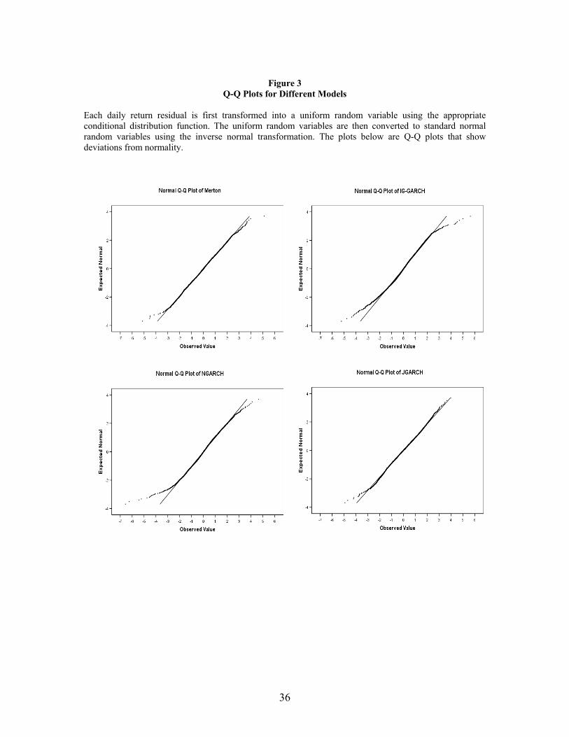
36

Figure 3

Q-Q Plots for Different Models

Each daily return residual is first transformed into a uniform random variable using the appropriate conditional distribution function. The uniform random variables are then converted to standard normal random variables using the inverse normal transformation. The plots below are Q-Q plots that show deviations from normality.

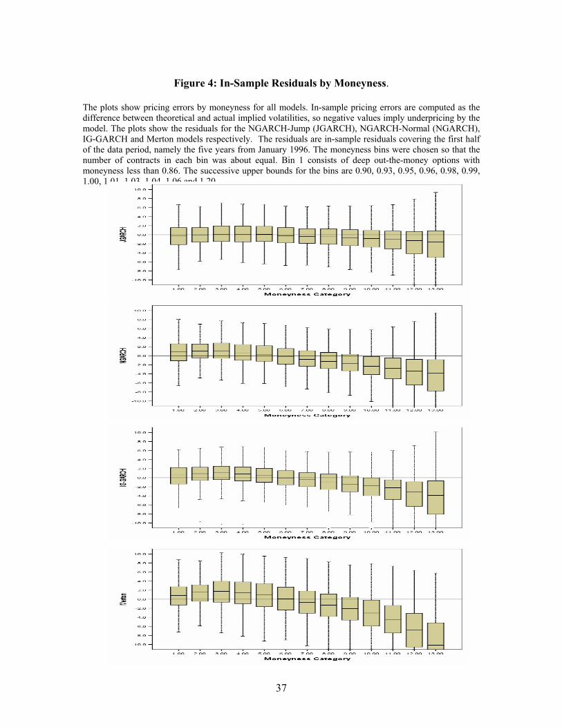
37

Figure 4: In-Sample Residuals by Moneyness.

The plots show pricing errors by moneyness for all models. In-sample pricing errors are computed as the difference between theoretical and actual implied volatilities, so negative values imply underpricing by the model. The plots show the residuals for the NGARCH-Jump (JGARCH), NGARCH-Normal (NGARCH), IG-GARCH and Merton models respectively. The residuals are in-sample residuals covering the first half of the data period, namely the five years from January 1996. The moneyness bins were chosen so that the number of contracts in each bin was about equal. Bin 1 consists of deep out-the-money options with moneyness less than 0.86. The successive upper bounds for the bins are 0.90, 0.93, 0.95, 0.96, 0.98, 0.99, 1.00, 1.01, 1.03, 1.04, 1.06 and 1.20.

38

Figure 5: Maturity Bias by Four Models

The figure shows box-whisker plots of the pricing errors produced by maturity for four models. In-sample errors are computed as the difference between theoretical and actual implied volatilities, so negative values imply underpricing by the model. For each maturity bucket there are four box plots ordered from left to right by the Merton model, the IG-GARCH model, the NGARCH-Normal model and the NGARCH-Jump model. The residuals are in-sample residuals covering the first half of the data period, namely the five years from January 1996. The contracts with maturities exceeding 90 days were not used in estimation, and thus can be viewed as out-of-sample residuals.

39

Figure 6: Time Series of Implied Volatilities for Each Model For each month we obtain the theoretical prices for all contracts within one half percent of the index value. We update the volatility process daily based on the realized index price. Given the theoretical option prices we compute the Black-Scholes implied volatility for each contract. For each model we compute the average Black-Scholes implied volatility for the month. The time series of these averages are compared with the actual average Black-Scholes volatilities for the month. The first figure is the Merton model, where the volatility is constant; the second figure is for the NGARCH-Normal model; the next figure is the IG-GARCH model and the bottom figure is the NGARCH-Jump model.

0

0.1

0.2

0.3

0.4

0 20 40 60 80 100 120

0

0.1

0.2

0.3

0.4

0 20 40 60 80 100 120

0

0.1

0.2

0.3

0.4

0 20 40 60 80 100 120

0

0.1

0.2

0.3

0.4

0 20 40 60 80 100 120

40

Figure 7: Residuals by Year and by Model

The figure shows the box plots of the residuals for at-the-money contracts for each model and for each year in the in-sample period for the first 5 years through year 2000, and in the out-of-sample period for the next 5 years. The box plots in each year are from left to right are the NGARCH-Jump, NGARCH-Normal, IG-GARCH, and Merton models, respectively. The parameters are estimated using option contracts with expiry dates less than 90 days over the period 1996 through 2000. The residuals used to compute the box plots are based off all contracts within one half percent of the strike price. The out-of-sample prices obtained after 2000 are based on parameters estimated using the data up through 2000.

41

Figure 8: Relative Out-of-Sample Performance of Models over Time The top figure shows the time series of monthly ratios of MSEs of the NGARCH-Normal (dashed line) and IG-GARCH (solid line) relative to the MSE of the NGARCH-Jump model. Panel B shows the time series of the monthly ratios of the MSEs of the IG-GARCH model relative to the MSEs of the NGARCH-Normal model. Ratios bigger than 1 indicate the superiority of the numeraire model. Month number starts from the first out-of-sample month in January 2001.

0

1

2

3

4

0 10 20 30 40 50 60

Out of Sample Month Number

MS

E(m

odel

)/MS

E(J

GA

RCH

)

0

1

2

3

4

5

0 10 20 30 40 50 60

Out of Sample Month Number

MSE

(IG)/M

SE(N

GAR

CH)

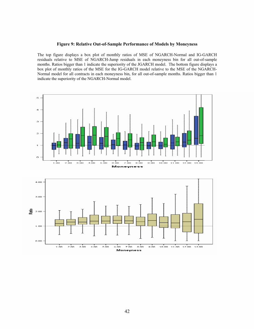
42

Figure 9: Relative Out-of-Sample Performance of Models by Moneyness The top figure displays a box plot of monthly ratios of MSE of NGARCH-Normal and IG-GARCH residuals relative to MSE of NGARCH-Jump residuals in each moneyness bin for all out-of-sample months. Ratios bigger than 1 indicate the superiority of the JGARCH model. The bottom figure displays a box plot of monthly ratios of the MSE for the IG-GARCH model relative to the MSE of the NGARCH-Normal model for all contracts in each moneyness bin, for all out-of-sample months. Ratios bigger than 1 indicate the superiority of the NGARCH-Normal model.

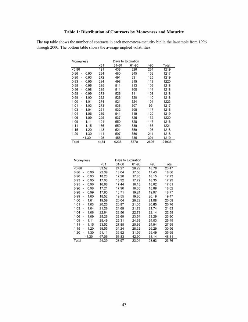
43

Table 1: Distribution of Contracts by Moneyness and Maturity The top table shows the number of contracts in each moneyness-maturity bin in the in-sample from 1996 through 2000. The bottom table shows the average implied volatilities.

Moneyness <31 31-60 61-90 >90 Total

<0.86 191 438 326 264 12190.86 - 0.90 234 480 345 158 12170.90 - 0.93 272 491 331 125 12190.93 - 0.95 294 498 315 113 12200.95 - 0.96 285 511 313 109 12180.96 - 0.98 285 511 308 114 12180.98 - 0.99 273 526 311 108 12180.99 - 1.00 262 526 320 110 12181.00 - 1.01 274 521 324 104 12231.01 - 1.03 273 538 307 99 12171.03 - 1.04 261 532 308 117 12181.04 - 1.06 239 541 319 120 12191.06 - 1.09 225 537 326 132 12201.09 - 1.11 191 550 328 147 12161.11 - 1.15 166 550 339 166 12211.15 - 1.20 143 521 359 195 12181.20 - 1.30 141 507 356 214 1218 >1.30 125 458 335 301 1219Total 4134 9236 5870 2696 21936

Days to Expiration

Moneyness <31 31-60 61-90 >90 Total

<0.86 33.52 24.27 20.29 18.78 23.470.86 - 0.90 22.39 18.04 17.56 17.43 18.660.90 - 0.93 18.23 17.28 17.85 18.15 17.730.93 - 0.95 17.03 16.92 17.72 18.35 17.290.95 - 0.96 16.88 17.44 18.18 18.62 17.610.96 - 0.98 17.21 17.90 18.65 18.89 18.020.98 - 0.99 17.85 18.71 19.24 19.97 18.770.99 - 1.00 18.52 19.55 19.86 20.19 19.471.00 - 1.01 19.59 20.04 20.29 21.08 20.091.01 - 1.03 20.25 20.87 21.05 20.65 20.761.03 - 1.04 21.29 21.69 21.79 21.74 21.631.04 - 1.06 22.64 22.56 22.73 22.14 22.581.06 - 1.09 25.26 23.69 23.54 23.29 23.901.09 - 1.11 28.49 25.31 24.69 24.03 25.491.11 - 1.15 33.52 27.85 25.93 24.94 27.691.15 - 1.20 39.55 31.24 28.32 26.29 30.561.20 - 1.30 51.11 36.92 31.56 29.49 35.69 >1.30 67.06 53.83 42.90 38.14 48.31Total 24.39 23.97 23.04 23.63 23.76

Days to Expiration

44

Table 2: Parameter Estimates from the Time Series of Daily Returns The tables report the parameter estimates for the models based on time series over the time period starting in 1970 and over two sub-samples. The Merton and NGARCH-Jump models are their restricted versions.

Estimate Std. Dev. Estimate Std. Dev. Estimate Std. Dev. Estimate Std. Dev.β0 2.73E-05 6.06E-07 1.13E-06 7.81E-08 1.71E-07 1.99E-08 -1.44E-06 1.661E-08β1 9.08E-01 2.11E-03 0.91946 0.0033 -19.13300 5.819E-13β2 5.62E-02 1.21E-03 0.04843 0.0012 4.08E-06 1.277E-10β3 2.47E+07 2.305E-19c 6.60E-01 1.20E-02 0.67556 0.0124

bρ -0.08347 6.71E-03 -0.03960 0.00327λ 0.61160 1.60E-02 2.26560 0.0047γ 1.9728 1.02E-02 1.35490 0.0073µ -0.12294 7.86E-03 -0.0733 0.0107

δ -2.56E-01 0.0141

η -6.20E-04 1.070E-07

ν 1614.5 4.410E-14

ML Value 29745.3 30297.4 30457.6 30238.3AIC Test -59480.6 -60584.8 -60899.2 -60464.6

Estimate Std. Dev. Estimate Std. Dev. Estimate Std. Dev. Estimate Std. Dev.β0 3.48E-05 2.99E-07 1.62E-06 2.58E-08 1.34E-07 3.42E-09 3.32E-08 2.232E-09β1 8.89E-01 7.59E-04 0.90912 0.0011 -19.20300 1.630E-13β2 6.39E-02 7.77E-04 0.05407 0.0009 4.10E-06 3.438E-11β3 2.47E+07 1.311E-19c 7.22E-01 6.42E-03 0.71245 0.0039

bρ -0.06888 2.28E-03 -0.04088 0.00139λ 0.50025 7.56E-03 2.27930 0.0037γ 1.9412 5.07E-03 1.7435 0.0024µ -0.091127 4.74E-03 -0.35940 0.0026

δ -1.07E-01 0.0021

η -6.14E-04 2.581E-08

ν 1632.4 5.645E-15

ML Value 21258.9 21595.2 21755.3 21560.8AIC Test -42507.8 -43180.4 -43494.6 -43109.6

Estimate Std. Dev. Estimate Std. Dev. Estimate Std. Dev. Estimate Std. Dev.β0 2.74E-05 2.12E-07 1.15E-06 1.26E-08 1.82E-07 2.47E-09 1.66E-08 2.155E-09β1 8.86E-01 5.07E-04 0.88888 0.0007 -19.17000 9.200E-14β2 5.64E-02 4.19E-04 0.05509 0.0004 4.07E-06 3.498E-11β3 2.47E+07 7.312E-20c 9.41E-01 6.63E-03 0.92969 0.0017

bρ -0.05992 3.05E-03 -0.03169 0.00129λ 0.70446 6.77E-03 2.39300 0.0030γ 1.9441 2.56E-03 1.3460 0.0008µ -0.10091 5.30E-03 -0.13336 0.0032

δ -3.94E-01 0.0008

η -6.08E-04 2.258E-08

ν 1647.4 6.145E-15

ML Value 13060.4 13407.6 13464.7 13369.9AIC Test -26110.8 -26805.2 -26913.4 -26727.8

1. Sample: 1/2/1970 - 12/30/2005

2. Sample: 1/2/1980 - 12/30/2005

3. Sample: 1/2/1990 - 12/30/2005

JGARCH IG-GARCHParameter

Merton NGARCH

NGARCH IG-GARCHJGARCHParameter Merton

JGARCH IG-GARCHParameter

Merton NGARCH

45

Table 3: Descriptive Statistics on Residuals for Time Series Models The top table reports descriptive statistics on the normalized residuals for the four different time series models. If the models are appropriately specified, the residuals should be standard normal random variables. The bottom table presents the Ljung-Box tests on the residuals and squared residuals for lags of up to 5 business days. The tests of hypothesis on no autocorrelation were conducted at the 5% level, and the significant values are indicated with stars. In addition to the full sample, tests are done in the two sub-periods after the stock market crash in October 1987.

Descriptive Statistics of Normalized Residuals

Ljung-Box tests for autocorrelation on residuals and squared residuals

Residual Merton NGARCH JGARCH IG-GARCHmean 0.003 0.000 0.001 -0.009std 1.048 0.991 1.067 0.980max 5.106 4.652 3.972 5.623min -5.135 -6.570 -4.927 -5.222skew 0.019 -0.152 -0.005 -0.172excess kurtosis 0.248 1.247 -0.111 1.198

Test of Normality Kolmogorov-Smirnov Statistic 0.012 0.025 0.010 0.033p value 0.005 0.000 0.027 0.000

1970-2005

Lag Auto- Box-Ljung Auto- Box-Ljung Auto- Box-Ljung Auto- Box-Ljung Correlation Statistic Correlation Statistic Correlation Statistic Correlation Statistic

1 0.099 89.91* 0.093 78.66* 0.099 89.44* 0.072 47.34*2 -0.002 89.94* -0.004 78.81* -0.001 89.46* -0.025 53.04*

Residuals 3 -0.011 91.01* -0.011 79.86* -0.011 90.52* -0.021 57.07*4 -0.012 92.30* -0.011 80.95* -0.012 91.84* -0.016 59.26*5 -0.010 93.16* -0.008 81.51* -0.010 92.70* -0.003 59.37*

1 0.019 3.294 0.051 23.23* 0.014 1.775 0.110 109.93*2 0.004 3.414 0.040 37.54* 0.000 1.776 0.160 343.32*3 0.002 3.439 0.029 45.03* -0.001 1.779 0.096 426.66*4 -0.003 3.514 0.010 45.91* -0.004 1.914 0.034 437.31*5 0.005 3.709 0.044 63.28* 0.003 2.000 0.158 663.32*

1988-1995

Lag Auto- Box-Ljung Auto- Box-Ljung Auto- Box-Ljung Auto- Box-Ljung Correlation Statistic Correlation Statistic Correlation Statistic Correlation Statistic

1 0.036 2.612 0.029 1.721 0.036 2.569 0.022 0.9532 -0.001 2.613 -0.002 1.728 -0.002 2.574 -0.014 1.340

Residuals 3 -0.039 5.760 -0.041 5.196 -0.039 5.638 -0.047 5.8814 -0.029 7.520 -0.021 6.132 -0.031 7.584 -0.009 6.0315 -0.017 8.106 -0.016 6.637 -0.018 8.235 -0.015 6.497

1 0.004 0.027 0.014 0.403 0.019 0.716 0.068 9.40*2 -0.009 0.186 -0.008 0.526 -0.002 0.727 0.028 10.96*3 -0.014 0.558 -0.010 0.713 -0.008 0.858 0.029 12.67*4 -0.004 0.592 -0.001 0.714 0.005 0.913 0.032 14.80*5 -0.007 0.690 0.008 0.833 -0.005 0.964 0.068 24.19*

1996-2005

Lag Auto- Box-Ljung Auto- Box-Ljung Auto- Box-Ljung Auto- Box-Ljung Correlation Statistic Correlation Statistic Correlation Statistic Correlation Statistic

1 0.011 0.320 0.008 0.171 0.012 0.344 -0.014 0.4602 -0.012 0.663 -0.013 0.568 -0.011 0.663 -0.027 2.359

Residuals 3 -0.026 2.425 -0.026 2.213 -0.026 2.387 -0.028 4.3084 -0.014 2.952 -0.007 2.355 -0.014 2.871 0.006 4.3855 -0.034 5.872 -0.035 5.370 -0.034 5.753 -0.041 8.643

1 -0.025 1.546 0.004 0.043 -0.027 1.889 0.186 86.89*2 0.026 3.217 0.044 4.867 0.024 3.382 0.187 175.50*3 -0.007 3.352 0.008 5.032 -0.009 3.571 0.176 253.38*4 0.009 3.567 0.012 5.421 0.009 3.784 0.120 289.99*5 0.015 4.170 0.040 9.451 0.015 4.378 0.181 372.58*

Squared Residuals

Merton

Squared Residuals

JGARCH IG-GARCH NGARCH Merton

Squared Residuals

JGARCH IG-GARCH NGARCH

JGARCH IG-GARCH NGARCH Merton

46

Table 4: Estimates Using Time Series and Options The parameter estimates based on the time series analysis were used as initial starting points for the panel estimation optimization problem, where option prices were incorporated into the analysis. The options used were restricted to contracts within 5% of the strike and maturities less than 90 days. Option prices were taken monthly, and incorporated with daily return data as discussed in the text. The data used spanned the period from January 1996 through to December 2000. For each model we report the point estimates, the standard deviations, the log-likelihood function (ML-value) and the Akaike Information Criterion (AIC)

Estimate Std. Dev. Estimate Std. Dev. Estimate Std. Dev. Estimate Std. Dev.β0 1.38E-04 2.28E-06 2.34E-06 1.06E-08 1.59E-07 1.81E-08 9.33E-09 1.592E-06β1 0.92994 6.23E-04 0.95110 0.0004 -19.47 6.118E-01β2 0.03600 3.35E-04 0.03004 0.0051 3.89E-06 4.717E-08β3 2.68E+07 1.739E+06c 0.73599 0.085 -0.07674 0.0958

bρ -0.07033 3.57E-01 -0.06254 0.08321 -0.40798 0.1808λ 0.91867 1.12E+00 0.38638 0.0722γ 5.28E-07 4.91E-05 4.32200 0.2603µ 0.3295 3.59E-02 -2.0920 0.9460

δη -5.99E-04 1.068E-05η∗ -5.92E-04 1.095E-05

ν 1649.4 2.937E+01

γ 9.3426E-07 2.69E-11 0.41392 0.6866Κ0 0.89314 1.09E+00 1.18600 0.2239ω 0.041002 6.07E-07 0.02920 0.000054338 0.02469 5.063E-05 0.02819 9.155E-05

ML Value 3821.10 4533.90 4852.10 4465.05AIC Test -7634.20 -9063.80 -9690.20 -8922.10

1/1996-12/2000

JGARCH IG-GARCHParameter Merton NGARCH

47

Table 5: Pairwise Comparisons of Models We compute the residuals for each contract using different models. For each pair of models, we record which model produces the smaller absolute residual. We report the proportion of times the model indicated first, produces smaller absolute errors than the model indicated second. For example, for deep in the money contracts with maturities exceeding 90 days, the NGARCH-Jump (JGARCH) model beat the NGARCH-Normal (NGARCH) model in the in-sample period 59% of the time. Values significantly different from 50% are bold-faced.

Expiry deep out out at in deep in Total Expiry deep out out at in deep in Total

<30 0.47 0.57 0.53 0.64 0.73 0.58 <30 0.47 0.66 0.51 0.44 0.60 0.5330-60 0.55 0.53 0.59 0.68 0.75 0.64 30-60 0.54 0.69 0.54 0.44 0.60 0.5761-90 0.59 0.54 0.59 0.62 0.65 0.61 61-90 0.58 0.63 0.53 0.48 0.60 0.58>90 0.61 0.48 0.47 0.50 0.62 0.59 >90 0.64 0.59 0.51 0.44 0.57 0.60Total 0.55 0.54 0.57 0.64 0.70 0.61 Total 0.56 0.67 0.53 0.44 0.59 0.57

<30 0.46 0.49 0.53 0.66 0.74 0.58 <30 0.58 0.71 0.63 0.49 0.66 0.6230-60 0.51 0.52 0.61 0.69 0.75 0.64 30-60 0.61 0.76 0.70 0.57 0.67 0.6561-90 0.58 0.56 0.59 0.63 0.71 0.63 61-90 0.63 0.72 0.70 0.63 0.66 0.66>90 0.61 0.61 0.54 0.68 0.75 0.67 >90 0.71 0.80 0.74 0.71 0.64 0.69Total 0.53 0.53 0.58 0.67 0.74 0.63 Total 0.63 0.74 0.69 0.57 0.66 0.65

<30 0.54 0.61 0.65 0.68 0.86 0.67 <30 0.67 0.87 0.82 0.81 0.85 0.7830-60 0.60 0.67 0.70 0.72 0.89 0.75 30-60 0.71 0.86 0.82 0.82 0.87 0.8061-90 0.62 0.67 0.70 0.74 0.89 0.76 61-90 0.75 0.81 0.81 0.83 0.88 0.81>90 0.66 0.79 0.74 0.68 0.92 0.80 >90 0.73 0.83 0.81 0.70 0.84 0.78Total 0.60 0.67 0.69 0.71 0.89 0.74 Total 0.72 0.85 0.82 0.81 0.87 0.80

<30 0.45 0.45 0.47 0.55 0.49 0.47 <30 0.61 0.63 0.66 0.57 0.46 0.5730-60 0.49 0.49 0.43 0.44 0.48 0.47 30-60 0.63 0.78 0.71 0.65 0.54 0.6361-90 0.53 0.53 0.47 0.45 0.50 0.50 61-90 0.65 0.75 0.72 0.66 0.54 0.63>90 0.55 0.58 0.51 0.54 0.54 0.55 >90 0.65 0.80 0.76 0.78 0.58 0.65Total 0.50 0.50 0.46 0.48 0.49 0.49 Total 0.64 0.74 0.70 0.64 0.53 0.62

<30 0.56 0.65 0.65 0.57 0.64 0.61 <30 0.70 0.86 0.83 0.80 0.67 0.7430-60 0.61 0.66 0.62 0.62 0.73 0.66 30-60 0.70 0.85 0.83 0.81 0.75 0.7661-90 0.61 0.65 0.63 0.67 0.80 0.70 61-90 0.73 0.81 0.81 0.82 0.81 0.78>90 0.63 0.80 0.81 0.69 0.85 0.77 >90 0.65 0.85 0.84 0.76 0.83 0.74Total 0.60 0.67 0.65 0.63 0.75 0.68 Total 0.70 0.84 0.82 0.80 0.76 0.76

<30 0.59 0.72 0.71 0.70 0.64 0.65 <30 0.65 0.89 0.85 0.82 0.72 0.7530-60 0.64 0.74 0.68 0.64 0.72 0.69 30-60 0.67 0.85 0.85 0.80 0.77 0.7561-90 0.65 0.71 0.69 0.69 0.80 0.72 61-90 0.74 0.79 0.75 0.76 0.80 0.76>90 0.63 0.71 0.67 0.65 0.82 0.73 >90 0.65 0.78 0.71 0.56 0.75 0.69Total 0.63 0.72 0.69 0.67 0.75 0.70 Total 0.68 0.84 0.82 0.78 0.77 0.75

In-Sample Comparisons Out-Sample Comparisons

NGARCH vs Merton

IG-GARCH vs Merton

JGARCH vs NGARCH

JGARCH vs IG-GARCH

JGARCH vs Merton

NGARCH vs IG-GARCH

NGARCH vs Merton

IG-GARCH vs Merton

JGARCH vs NGARCH

JGARCH vs IG-GARCH

JGARCH vs Merton

NGARCH vs IG-GARCH