j. d. freels a. j. baker investigation of 1d compressible

J. D. Freels1 · A. J. Baker2

Investigation of 1D Compressible Navier-Stokes Equations usingCOMSOL Multiphysics Equation-Based Modeling

Abstract A fundamentally important area of the COMSOL Mul-tiphysics platform is that of equation-based modeling. This rootcapability is unique in commercially available codes and offersunlimited application. One specific area that requires more de-tail, even in the CFD Module of COMSOL, is that of 1D Com-pressible Navier Stokes (NS) equations. The stabilization meth-ods developed and demonstrated in 1D, can then be utilized inboth 2D and 3D in a confident manner. Over 28 years ago, theseequations were investigated, and also extended to 2D[1]. Themethods developed therein have been significantly improved, aswill be published in an upcoming monograph[2]. The advance-ments discussed are primarily concerned with the method of sta-bilization. Equations as input into the COMSOL general formPDE in non-dimensional weak form are discussed and presented.Both the Taylor Weak Statement (TWS)[1] and Filtered analyt-ically Navier-Stokes (FaNS)[2] are implemented for 1D com-pressible NS equations. Results for Viscous Burger’s Equationand Riemann Shock Tube benchmarks are compared directlybetween the TWS and FaNS methods. A 2D approximation isimplemented for the shock tube problem using the COMSOLCFD module high Mach number, laminar flow physics settings.Dimensional-form and non-dimensional-form models are devel-oped as separate components, allowing for the COMSOL consis-tent (CC) stabilization method and compared to TWS and FaNS.An ultimate goal of this work is to incorporate the TWS andFaNS stabilization methods as options for the COMSOL CFDmodule.

1 Introduction

It is well known within the field of numerically solving Navier-Stokes (NS) equations that the process is inherently unstable.Even an experienced users of popular commercial codes maynot realize this when stated to them. I had this happen to meonce while presenting this fact to a group of researchers whoshared the same project together. It was argued to me “the codeI use does not have any artificial dissipation !”

1 (retired) Oak Ridge National Laboratory (ORNL)Adjunct Faculty, The University of Tennessee, USAcell: (865)919-0320E-mail: [email protected]

2 Professor EmeritusThe University of Tennessee, USAcell: (865)207-1537E-mail: [email protected]

A very important feature of COMSOL Multiphysics in solv-ing NS equations is to distinguish between “consistent” and “in-consistent” stabilization methods provided. If the user reviewsthe “inconsistent” methods, he should be aware that his resultsare probably not valid for a real-world application, but may offera way to achieve an ultimately “consistent” solution; i.e., a stepalong the way.

The “inconsistent” method is described in the COMSOL doc-umentation as using established methods in the industry.[3] Fur-ther, using this “inconsistent method adds a certain amount ofdiffusion independently of how close the numerical solution isto the exact solution.” The “inconsistent” methods are well doc-umented in the COMSOL manuals and consistent with that pub-lished in the literature. The COMSOL input provides full con-trol, through direct input in the graphical user interface (GUI) orby modifying the equations available to the user.

The “consistent” methods are described in the COMSOLmanuals as being based on methods referenced, but no additionaldescription given, nor any way to examine or change it (i.e., notshown in equation view) other than to turn it off and on; withthe default being on. These methods are split into streamline andcrosswind diffusion with recommendations on how to use them.This is understandable given the proprietary nature of the COM-SOL commercial product and the high quality of the results.

The external stabilization methods described and results pre-sented herein turn “off” both the “inconsistent” and “consistent”COMSOL methods, except where explicitly turning “on” the“consistent” COMSOL method (CC) where it is needed to com-pare to the external stabilization methods presented.

2 Compressible Navier-Stokes - Specific Conservative Form

A conservative, non-dimensional form of the compressible NSequations is derived in detail.[1] The resulting full 3D conservation-law equations of mass, momentum, and energy are concisely

shown below in index notation.

L (ρ) =∂ρ

∂ t+

∂mi

∂xi= 0,

L (mi) =∂mi

∂ t+

∂ (u jmi)

∂x j+Eu

∂ p∂xi

+∂

∂x j

[µe

Re

(∂ui

∂x j+

∂u j

∂xi

)− 2

3µe

Re∂uk

∂xkδi j

]= 0,

L (g) =∂g∂ t

+∂ (uig)

∂xi+2EcEu

∂ p∂ρ

∂mi

∂xi− ∂

∂xi

(ke

PrRe∂T∂xi

)+

2EcRe

∂

∂xi

[u jµe

(∂ui

∂x j+

∂u j

∂xi− 2

3∂uk

∂xkδi j

)]= 0.

The non-dimensional scaling constants are defined as

– Euler number (Eu) = poρoa2

o

– Reynolds number (Re)= ρoaoLoµo

– Eckert number (Ec) = ρoa2o

2go

– Prandtl number (Pr) = µoCpoko

The independent variables are customary time (t) and space (xi).The dependent variables are listed and described here:

– momentum, mi = ρui,– total volume-specific enthalpy, g= ρH = ρ(e+∑i u2

i /2)+ p,– variables ρ,ui, p,T are density, velocity, pressure, and tem-

perature respectively,– internal energy, e =CpT ,– fluid properties, Cp,µ,k are specific heat at constant pres-

sure, dynamic viscosity, and thermal conductivity respectively,and

– the fluid turbulence is ignored in this investigation, allowingthe system of equations to be closed with µe = µ , and ke = k.

The reference variables, denoted by (o), are chosen consistentlyat a specific location in the geometry and the corresponding fluidequation of state is related back to the physical problem in di-mensional form.

The present COMSOL modeling is initially limited to 1D.We use the “General Form PDE” physics component, with unityalong the diagonal of the mass coefficient (time derivative). Allother entries are zero except for the conservative flux; the inputsare repeated below:

Γ1 =m1Γ2 =um1+Eu*p-4/3/Re*mu*d(u,x)Γ3 =ug+2*Ec*Eu*T*m1-2*Ec/Re*u*4/3*mu*d(u,x)-1/Re/Pr*k*d(T,x)

The variables um1 and ug are defined with other variables in thevariables section of the COMSOL model tree. The state vari-ables are those operated on by the time derivative, i.e., [ρ,m1,g],hence, additional closure is required for COMSOL to find a so-lution. This is accomplished by adding the “Domain ODEs andDAEs” physics component and inserting the following entries inthe source-terms section:

(g-Ec*m1*m1/rho)/Cp-pif(real_gas==0,1-Cp,mat1.def.Cp(T*T_o)/Cp_o-Cp)if(real_gas==0,T_ideal-T,T_real-T)

solving for p,Cp, and T , respectively. Note the simplicity of se-lecting ideal or real gas fluid properties based on the real_gasparameter setting, where T_ideal=p/rho, andT_real=p/(zv*(mat1.def.rho(p*p_o,T*T_o)/rho_o)) arealso defined in the variables section.

3 Stabilization Methods

As mentioned earlier, the stabilization provided internal to COM-SOL are the “consistent” and “inconsistent” methods. We havenot enabled the “inconsistent” method anywhere in this inves-tigation. Where desired to compare to the COMSOL “consis-tent” method, both streamline and crosswind diffusion is enabledwithin the high-speed Mach number laminar flow physics of theCFD module (hereafter referred to as the CFD module). Other-wise, when the TWS or FaNS stabilization method is used, theCC method is disabled, and the external stabilization (TWS orFaNS) is enabled through the use of weak-form PDE if equation-based physics, or weak contribution if CFD module physics.

One major new finding that came out of this investigationwith COMSOL is it appears that only the conservative formis required (a separate non-conservative form is not necessary)to generate the external stabilization methods (TWS or FaNS)when coupling to the non-conservative form of the governingequations as provided by the CFD module. This is because thetest function will generate a new unknown automatically by COM-SOL, and as long as the breakdown to non-conservative variablesis provided to COMSOL through the variables section, then thesystem is closed. This is a major simplification that allows for theidentical form of the external stabilization methods to be usedwith most any form of the NS equations provided in the CFDmodule.

3.1 Legacy Taylor Weak Statement (TWS)

A complete derivation of the TWS stabilization method for thisequation set is provided in Chapter 4 of Freels[1]. Table 1 ofChapter 4 of Baker[2] summarizes how this powerful methodrecovers many other widely used methods including those inCOMSOL. In this study, we focus on the β term and ignore allother terms in the full TWS. The net result is an equation of theform

TWSq =hβq

2uu

∂ 2q∂x2 ,

where

q = {ρ,m1,g},u is a unit vector and indicates the sign of u,h is the element measure which in 1D is the element length,

The implementation of TWS into COMSOL is accomplished us-ing the weak contribution settings

-test(rhox)*rhox*b_rho*ubar2-test(m1x)*m1x*b_m1*4*ubar2-test(gx)*gx*b_g*ubar2

where ubar2=max(u_min,abs(u))*dx/order*beta, andu_min=a minimum velocity to prevent instabilities near zero ve-locity regions, dx=element length (h), order=element basis or-der if the user desires higher order Lagrange basis function (2,

J. D. Freels and A. J. Baker of 7 COMSOL Conference 2020 North America, October 7-8

3, 4, etc.). beta=1/sqrt(15) (“optimal”). Note that the b_rho,b_m1, and b_g parameters are utilized to create per-state vari-able (βq) tweaking and are usually unity or less. In this study,we found a good set to be {6,7,12}/24.

3.2 Error Free CFD - the Filtered analytically Navier-Stokes(FaNS)

A generalized, multi-dimensional form for the FaNS stabiliza-tion method is provided by Baker[2]. A 1D reduction yields thefollowing equation

fdqdx− µ

Red2qdx2 −

Reh2

12µf

ddx

[f

dqdx

]= 0+O(h4)

Note the required presence of a physical viscous term for FaNS.Further, the added term for error annihilation also includes aReynolds number in the numerator! Because there is no viscousterm present in the continuity equation, there is no added FaNSterm generated therein. We recommend consideration be givento add the TWS βρ term for stability if needed for the continu-ity equation [L (ρ)]. However, based on experience from thisstudy, only the FaNS terms for momentum [L (m1)] and energy[L (g)] equations are required. In 1D, the FaNS terms used herereduce to

FaNS1D(m1) =Reh2

12µu2 d2m1

dx2

FaNS1D(g) =Re Prh2

12ku2 d2g

dx2

The extension to 2D (results not presented in this study) yieldthe following

FaNS2D(m1) =Reh2

12µ(u+ v)

[u

∂ 2m1∂x2 + v

∂ 2m1∂y2

]FaNS2D(m2) =

Reh2

12µ(u+ v)

[u

∂ 2m2∂x2 + v

∂ 2m2∂y2

]FaNS2D(g) =

Re Prh2

12k

[u2 ∂ 2g

∂x2 + v2 ∂ 2g∂y2

]The corresponding COMSOL inputs to the weak contributionsettings for 1D

-h^2/12*Re/mu*test(m1x)*u^2*m1x-h^2/12*Re*Pr/k_iso*test(gx)*u^2*gx

The companion 2D settings are also provided here-h^2/12*Re/mu*(u+v)*(test(m1x)*u*m1x+test(m1y)*v*m1y)-h^2/12*Re/mu*(u+v)*(test(m2x)*u*m2x+test(m2y)*v*m2y)-h^2/12*Re*Pr/k_iso*(test(gx)*u^2*gx+test(gy)*v^2*gy)

As discussed earlier, the above weak contributions for FaNS arewritten identically for the conservative form written in COM-SOL equation-based physics, or in non-conservative form in theCOMSOL CFD module for High Mach Number flow.

4 Validation

Three test cases are presented herein to start on a validation effortfor the new equation system {ρ,m,g} and stabilization methods(TWS or FaNS) for COMSOL.

a Viscous Burger’s Equation A viscous extension to the classi-cal Burger’s equation; perhaps the simplest, yet challenging,equations to solve in 1D.

b Riemann Shock Tube A more extensive simulation utilizingall three of the conservation laws (mass, momentum, and en-ergy), in a time-dependent mode of 1D; also a very com-mon, yet challenging problem to solve. A variation of thisproblem is included in the COMSOL v5.4 application library(shock tube.mph) which was used to begin our investigationinto equation-based modeling with COMSOL. However, thestabilization method used in this model file is obviously notthe CC method and of low quality. Further, instead of solv-ing a transient, this model file solves the time dependence asa 2nd spatial dimension; quite interesting, but not of interestin this investigation.

c The 1D Riemann Shock Tube problem is approximated asa 2D dimensionless model within the High Mach NumberFlow physics of the COMSOL CFD module. Both the TWSand FaNS stabilization methods are incorporated into thismodel as weak constraints. The COMSOL consistent stabi-lization method is then directly compared to TWS and FaNS.

The reader is encouraged to utilize a “zoom” feature of the brows-ing device in order to see the details of these validation results.

4.1 Viscous Burger’s Equation

A simplification of the more general 3D equation initially pre-sented, we assume 1D, steady-state, incompressible, isothermal,and isobaric, and hence, constant properties, which leaves thefollowing two terms in the momentum equation to solve

ududx− 1

Red2udx2 = 0

The domain is a horizontal line of unit length (0 ≤ x ≤ 1). Theboundary conditions are a pair of Dirichlet conditions on eachend point u(x = 0) = 1 and u(x = 1) =−1. The initial conditionsare set to u(0≤ x < 0.5) = 1, u(0.5 < x≤ 1.0) =−1, and u(x =0) = 0. The challenge is to stabilize the solution so that the finalcondition will be as near as possible the initial condition; sincethis is the exact solution for this problem as Reynolds numberapproaches infinity. We only investigate the FaNS stabilizationfor this particular test case.

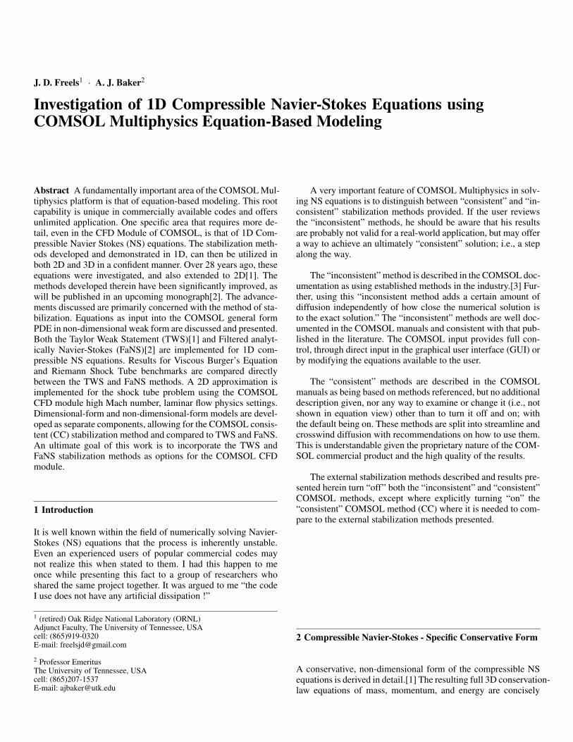
We initially solve using a uniform mesh, with fixed Reynoldsnumber, and utilize a parametric sweep on the number of ele-ments as shown in Figure 1 at Reynolds number 104. Figure 1(a)shows the entire solution field, while Figure 1(b) shows a mag-nified view of the top corner. Clearly the solution is convergingto the expected value, with no sign of instability, as the numberof elements is increased. The magnified view shows absolutelyno indication of overshoot and the solution is clearly approach-ing a “square wave” appearance. We next utilize a non-uniformmesh manually created about the center point with fixed numberof elements, and fixed Reynolds number as shown in Figure 2. Aparametric sweep on the element ratio is utilized with Reynoldsnumber 103, and the total number of elements equal 21. Fig-ure 2(a) shows the complete solution, while Figure 2(b) showsa magnified view of the top corner region. The result is clearlystable, and consistent with expected results. We have also clearlydemonstrated that a fixed element size is not required for FaNSto obtain a high-quality solution. Our final investigation shown


(a) overall view (b) magnified at discontinuity top

Fig. 1 Viscous Burger’s Equation Solution using FaNS Stabilization atRe = 104 for Varying Uniform Mesh Resolution.

(a) overall view (b) magnified at discontinuity top

Fig. 2 Viscous Burger’s Equation Solution using FaNS Stabilization atRe = 103 for Varying Non-Uniform Mesh Element Ratio at MaximumNumber of Elements = 21.

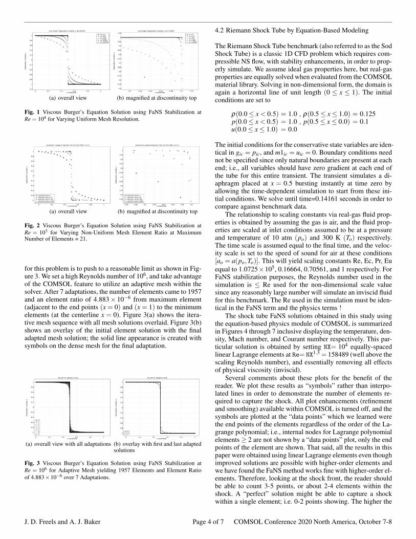
for this problem is to push to a reasonable limit as shown in Fig-ure 3. We set a high Reynolds number of 106, and take advantageof the COMSOL feature to utilize an adaptive mesh within thesolver. After 7 adaptations, the number of elements came to 1957and an element ratio of 4.883× 10−6 from maximum element(adjacent to the end points (x = 0) and (x = 1) to the minimumelements (at the centerline x = 0). Figure 3(a) shows the itera-tive mesh sequence with all mesh solutions overlaid. Figure 3(b)shows an overlay of the initial element solution with the finaladapted mesh solution; the solid line appearance is created withsymbols on the dense mesh for the final adaptation.

(a) overall view with all adaptations (b) overlay with first and last adaptedsolutions

Fig. 3 Viscous Burger’s Equation Solution using FaNS Stabilization atRe = 106 for Adaptive Mesh yielding 1957 Elements and Element Ratioof 4.883×10−6 over 7 Adaptations.

4.2 Riemann Shock Tube by Equation-Based Modeling

The Riemann Shock Tube benchmark (also referred to as the SodShock Tube) is a classic 1D CFD problem which requires com-pressible NS flow, with stability enhancements, in order to prop-erly simulate. We assume ideal gas properties here, but real-gasproperties are equally solved when evaluated from the COMSOLmaterial library. Solving in non-dimensional form, the domain isagain a horizontal line of unit length (0 ≤ x ≤ 1). The initialconditions are set to

ρ(0.0≤ x < 0.5) = 1.0 , ρ(0.5≤ x≤ 1.0) = 0.125p(0.0≤ x < 0.5) = 1.0 , p(0.5≤ x≤ 0.0) = 0.1u(0.0≤ x≤ 1.0) = 0.0

The initial conditions for the conservative state variables are iden-tical in gic = pic, and m1ic = uic = 0. Boundary conditions neednot be specified since only natural boundaries are present at eachend; i.e., all variables should have zero gradient at each end ofthe tube for this entire transient. The transient simulates a di-aphragm placed at x = 0.5 bursting instantly at time zero byallowing the time-dependent simulation to start from these ini-tial conditions. We solve until time=0.14161 seconds in order tocompare against benchmark data.

The relationship to scaling constants via real-gas fluid prop-erties is obtained by assuming the gas is air, and the fluid prop-erties are scaled at inlet conditions assumed to be at a pressureand temperature of 10 atm (po) and 300 K (To) respectively.The time scale is assumed equal to the final time, and the veloc-ity scale is set to the speed of sound for air at these conditions[ao = a(po,To)]. This will yield scaling constants Re, Ec, Pr, Euequal to 1.0725×105, 0.16664, 0.70561, and 1 respectively. ForFaNS stabilization purposes, the Reynolds number used in thesimulation is ≤ Re used for the non-dimensional scale valuesince any reasonably large number will simulate an inviscid fluidfor this benchmark. The Re used in the simulation must be iden-tical in the FaNS term and the physics terms !

The shock tube FaNS solutions obtained in this study usingthe equation-based physics module of COMSOL is summarizedin Figures 4 through 7 inclusive displaying the temperature, den-sity, Mach number, and Courant number respectively. This par-ticular solution is obtained by setting NX= 104 equally-spacedlinear Lagrange elements at Re= NX1.3 = 158489 (well above thescaling Reynolds number), and essentially removing all effectsof physical viscosity (inviscid).

Several comments about these plots for the benefit of thereader. We plot these results as “symbols” rather than interpo-lated lines in order to demonstrate the number of elements re-quired to capture the shock. All plot enhancements (refinementand smoothing) available within COMSOL is turned off, and thesymbols are plotted at the “data points” which we learned werethe end points of the elements regardless of the order of the La-grange polynomial; i.e., internal nodes for Lagrange polynomialelements≥ 2 are not shown by a “data points” plot, only the endpoints of the element are shown. That said, all the results in thispaper were obtained using linear Lagrange elements even thoughimproved solutions are possible with higher-order elements andwe have found the FaNS method works fine with higher-order el-ements. Therefore, looking at the shock front, the reader shouldbe able to count 3-5 points, or about 2-4 elements within theshock. A “perfect” solution might be able to capture a shockwithin a single element; i.e. 0-2 points showing. The higher the


Reynolds number used in the FaNS simulation, the nearer toperfect the algorithm will get. There is no customary “tuning”to perform to sharpen the solution, but the mesh requirementsdo go up along with Reynolds number. Hence, we refer to thisas the computational error being “annihilated”, or “CFD errorfree.” All the variables appear as expected for accuracy and con-sistency compared to known results. Note the maximum Courantnumber, shown as identical to the shape of the velocity in Figure7, is over 19 in this plot. This is impressive for such a demand-ing transient simulation using the normal BDF time-dependentsolver within COMSOL.

Fig. 4 Riemann Shock Tube Dimensionless Solution using COMSOL PDEInterface Physics, Re = 158489 and 104 Elements; temperature at final timeof 0.14161s.

Fig. 5 Riemann Shock Tube Dimensionless Solution using COMSOL PDEInterface Physics, Re = 158489 and 104 elements; density at final time of0.14161s.

Fig. 6 Riemann Shock Tube Dimensionless Solution using COMSOL PDEInterface Physics, Re = 158489 and 104 elements; Mach number at finaltime of 0.14161s.

Fig. 7 Riemann Shock Tube Dimensionless Solution using COMSOL PDEInterface Physics, Re = 158489 and 104 Elements; Courant number at thefinal time of 0.14161s.

4.3 Riemann Shock Tube by CFD Module

An eventual goal of this work is to incorporate alternative sta-bilization methods into the CFD module. One way to supportthis effort is to directly compare the existing CC method to boththe TWS and FaNS methods. We originally tried to perform thistask by converting the dimensionless form of the TWS or FaNSmethods into the default dimensional (SI) form of the High MachNumber (HMN) flow physics within the CFD module. This ini-tial attempt proved difficult, and we hope to get back to that ef-fort, since it should certainly be possible to do this. We thenfound better success by changing the default settings for CC SIunits to dimensionless form (select None for the units setting)which is a normal setting change available within COMSOL.Additional changes were also necessary to fully create the cor-rect dimensionless form: (1) change the ideal gas constant tounity, (2) input all variable definitions and initial conditions todimensionless values (divide by scaling factors), (3) divide dy-


namic viscosity by Re in it’s definition, and (4) divide thermalconductivity by Re*Pr in it’s definition.

Once the HMN is set up in dimensionless form, a few addi-tional steps are needed to be able to compare to the TWS andFaNS methods. Because the HMN does not have a 1D capability(only 2D and 3D are available), a 1D geometry is approximatedby defining the geometry to be a unit width in the 2nd Cartesiandirection (y) and only a single element high. Symmetry bound-ary conditions are set in the y direction for both (twin) horizontalboundaries (0→ 1). The transverse velocity, v, is also set to zeroeverywhere as a (probably unnecessary) Dirichlet constraint; ef-fectively taking the transverse velocity variable (v) out of theproblem (now 1D).

In performing a CC simulation with this model, we enablethe consistent stabilization check boxes on the GUI, and disableboth the TWS and FaNS weak contributions from operating. Toperform a TWS simulation with the same model, we disable theCC stabilization by unchecking the boxes on the GUI, and enablethe TWS weak contributions, and leave the FaNS weak contribu-tion disabled. And similarly, a FaNS simulation with this samemodel is performed by disabling both CC and TWS, and enablethe FaNS weak contributions.

It is important to emphasize that both TWS and FaNS havebeen coupled directly to the HMN through weak contributions.By definition, the CC stabilization method is only available withinthe activated CFD module, and not available through the equation-based modeling physics. Therefore, all three different stabiliza-tion methods are using exactly the same physics model (HMN ofthe CFD module) in every aspect except the change in choice ofstabilization method. We are not using the equation-based mod-eling in the remaining figures, except to generate the weak con-tribution setting entries for the TWS and/or FaNS stabilizationmethods. Further. all three methods are solving non-conservativestate variables {p,u,T}. During the TWS and FaNS stabiliza-tion simulations, because the weak contribution test functionsare written on the conservative variables {ρ,m1,g}, additionalalgebraic variables to define conservative variables as a functionof the non-conservative state variables are required to be definedin the variables section of the model tree. It is very impressivethat COMSOL provides this much flexibility to the user with thiscapability.

Results for the identical Riemann Shock Tube problem us-ing the HMN physics in the CFD module are shown in Figures 8through 10 for pressure, velocity, and Mach number respectively.Both the TWS and CC methods are forced to an inviscid condi-tion by setting the viscosity to near zero. The FaNS method issetup with Re= 1.0725× 105 which is a reasonable upper limitfor Re based on scaling factor. All simulations are using 10725fixed elements. All of these figures are shown as symbols withno connecting lines (CC black triangles, FaNS red circles, andTWS blue squares), without any additional smoothing, and di-rectly on the data points (end points or nodes of each element).Figures 8(a) and 9(a) show the overall view which, visually indi-cates an identical solution for all 3 stabilization methods. How-ever, when the magnified view is examined in Figures8(b), 9(b),and 10, a difference between the methods is detected. One dif-ference is that the 3 methods land on 3 different x-coordinatelocations. This is best explained by realizing that a large num-ber of time steps are required (105 → 106), and there is a vari-ation in time steps along the way as defined by the BDF time-stepping solver. Hence, it is certainly plausible that the cumula-tive time integration error could cause a slightly different end-

ing position for the shock front between the 3 different methods[0.005/(0.75− 0.33) ≈ 1.2%] This difference can only be at-tributed to the time-stepping algorithm and is not a direct func-tion of the stabilization method.

However, this small difference in landing position along the xaxis does provide the benefit of allowing for a clearer magnifiedview of this region. Looking at the shape of the magnified resultsin Figures 8(b) and 9(b), the TWS method appears to be morediffusive, and yet still undershoots the downstream side of theshock slightly. One could argue that additional diffusivity canbe removed by appropriate reduction in β factor, but this wouldalso tend to additionally undershoot at the price of less diffusiontoward overshoot in the upstream side. The CC method does agood job overall but produces the most severe undershoot on thedownstream side and a slight diffusion on the upstream side, TheCC method does show the least number of data points within theshock indicating good shock capture. The FaNS method is theonly method to show no undershoot in the downstream side, andshows the least level of diffusion in the upstream side. The FaNScould probably capture the shock with fewer elements if higherRe were used, or additional element refinement were providedabout the shock as was done in the Burger’s Equation study.

Perhaps the most enlightening result is that of Figure 10 show-ing the velocity overlay of the 3 methods in a magnified view ofthe shock plateau. Of particular interest is the “hump” in the ve-locity almost exactly midway across the plateau, which involvesabout [.008/0.25 ≈ 3.2%] of the plateau span. This “hump” oc-curs as a result of the contact discontinuity created by the instan-taneous transition of the simulated event at time zero. The FaNSsimulation shows a smooth transition of the velocity across thisregion while maintaining consistent (equal) value of the veloc-ity (flat profile) on each side of the hump. The CC method hasdifficulty capturing this hump, indeed, shows a chaotic oscilla-tory pattern all across the velocity profile in this plateau region.The TWS method shows a smooth transition, but also causes thevelocity to be slightly different between either side of the hump.We studied this phenomena further by decreasing the conver-gence residual level and discovered that the lowest level that CCcould go was about 1.0×10−4 while both TWS and FaNS couldgo at least down to 1.0×10−6. In an effort to create a fair com-parison, the convergence criteria of all three methods was set to1.0×10−4 and the setting used in the results shown in Figure 10.Further, we magnified the plateau region of all 3 methods evenfurther and realized that all 3 methods had some level of oscilla-tion, but CC showed the greatest level by a large extent as can beseen in Figure10. We also went back to the shock tube solutionsobtained using the conservative equations with equation-basedphysics, and discovered that these oscillations did not exist at allthere. Therefore, we attributed the issue (chaotic oscillatory na-ture of the plateau region) to the non-conservative form of theequations, the choice of state variables, and the iterative mannerin which density is solved via the equation of state rather than thecontinuity equation. While both TWS and FaNS reduced this os-cillation, it is omnipresent in all the stabilization methods used inthis HMN study, and is likely to be the cause of the CC methodnot being able to have a residual smaller than 1.0×10−4.

5 Conclusions and Suggested Further Research

We have developed a better understanding of how to build equation-based models in COMSOL. The steps required to create dimen-


(a) full view (b) magnified view at shock front

Fig. 8 Riemann Shock Tube Dimensionless Solution using COMSOL HighMach Number Flow CFD Module, Re = 1.0725×105 and 10725 Elements;pressure comparison between CC (black triangle), TWS (blue square), andFaNS (red circle) at final Time of 0.14161s.

(a) full view (b) magnified view at shock front

Fig. 9 Riemann Shock Tube Dimensionless Solution using COMSOL HighMach Number Flow CFD Module, Re = 1.0725×105 and 10725 Elements;velocity comparison between CC (black triangle), TWS (blue square), andFaNS (red circle) at final time of 0.14161s.

sionless conservative-form compressible NS equations in 1D havebeen completed {ρ,m1,g}. Conversion of dimensional non- con-servative CFD module physics-based models to dimensionlessform has been established {p,u,T}. Coupling of two externalstabilization methods, legacy TWS and recent FaNS, to dimen-sionless form, both conservative and non-conservative equationsets, has been completed and demonstrated to be consistent withknown results and extremely accurate. The coupling of the sta-bilization methods has been performed in such as way as to beeasily enabled and disabled independently of each other. Com-parison between the three stabilization methods (CC, TWS, andFaNS) has been demonstrated with advantages and disadvan-tages of each method highlighted.

We intend to transform the working models in this paper toan application, created from the COMSOL application builder,and donate through the COMSOL exchange feature. This willaccomplish a goal to learn and use the application builder, andserve a purpose to allow interested readers to investigate inde-pendently with the methods described herein.

While not shown in this paper, some additional COMSOLmodel development of compressible NS equations in dimension-less conservative form has been completed in 2D with limiteddemonstration. We intend to complete the 2D development, in-cluding turbulence modeling and extend the application. An ex-tension to 3D will then be possible in a straight forward mannergiven the flexibility and capability of the COMSOL equation-based framework. Assuming the success of a 3D implementa-tion, and the computing constraints required thereof, a natural

Fig. 10 Riemann Shock Tube Dimensionless Solution using COMSOLHigh Mach Number Flow CFD Module, Re = 1.0725× 105 and 10725Elements; velocity comparison between CC (black triangle), TWS (bluesquare), and FaNS (red circle) at final time of 0.14161s [magnified view atshock plateau].

extension will be to develop a parabolized NS capability as wasoriginally discussed in Freels[1], and developed[4],[5] and archived[6] many years ago. These new developments could then be com-bined with the external stabilization methods shown in this paperto enhance the COMSOL CFD capability.

Acknowledgements We would like to acknowledge the developers, andtechnical support personnel at COMSOL for providing a superb tool forbuilding, simulating, and investigating finite-element based CFD models,and multiphysics models in general.

References

1. Freels, J. D., “A Taylor Weak-Statement Finite Element Algorithm forReal-Gas Computational Fluid Dynamics,” A Dissertation Presentedfor the Doctor of Philosophy Degree, The University of Tennessee,Knoxville, May, 1992.

2. Baker, A. J., CFD Error Annihilation: Discretization, Difference Alge-bra, Physics-based Modeling, Numerical Linear Algebra, with OptimalFE Constructions, Elsevier Inc., Suite 800, 230 Park Avenue, New York,NY, in press 2020.

3. COMSOL, Inc., 100 District Avenue, Burlington, MA 01803 USA,COMSOL-5.5, a product of COMSOL, Inc., [email protected].

4. Baker, A. J. and Freels, J. D., “A Comprehensive PNS Upgrade forThree-Dimensional Reentry Flow Prediction,” Tech. Rep. COMCO TR88-4.0, Computational Mechanics Corporation, June 1988, Final Report,AF/BMO SBIR Phase I Contract F04704-87-C-0100.

5. Baker, A. J., Freels, J. D., Iannelli, G. S., and Manhardt, P. D., “A FiniteElement Code for Real Gas Aerodynamics Simulation (PRaNS),” Tech.Rep. BMO:TR-91-39, Computational Mechanics Corporation, 1994,Vol. I Algorithm and Theory.

6. Baker, A. J., Optimal Modified Continuous Garlerkin CFD, John Wi-ley & Sons Ltd., The Atrium, Southern Gate, Chichester, West Sussex,PO19 8SQ, United Kingdom, 2014.


j. d. freels a. j. baker investigation of 1d compressible

Documents