it's not easy being green: the evolution of galaxy...

Colour evolution in EAGLE 1

It’s not easy being green: The evolution of galaxy colour inthe EAGLE simulation

James W. Trayford1?, Tom Theuns1, Richard G. Bower1, Robert A. Crain2,Claudia del P. Lagos3,4, Matthieu Schaller1, Joop Schaye51Institute for Computational Cosmology, Durham University, South Road, Durham, DH1 3LE.2Astrophysics Research Institute, Liverpool John Moores University, 146 Brownlow Hill, Liverpool, L3 5RF.3International Centre for Radio Astronomy Research, 7 Fairway, Crawley, 6009, Perth, WA, Australia.4Australian Research Council Centre of Excellence for All-sky Astrophysics (CAASTRO), 44 Rosehill Street Redfern,

NSW 2016, Australia.5Leiden Observatory, Leiden University, P.O. Box 9513, 2300 RA Leiden, the Netherlands.

23 May 2016

ABSTRACTWe examine the evolution of intrinsic u-r colours of galaxies in the eagle cosmological hydrodynam-ical simulations, which has been shown to reproduce the observed redshift z = 0.1 colour-magnitudedistribution well, with a focus on z < 2. The median u-r of star-forming (‘blue cloud’) galaxiesreddens by 1 magnitude from z = 2 to 0 at fixed stellar mass, as their specific star formation ratesdecrease with time. A red sequence starts to build-up around z = 1, due to the quenching of low-mass satellite galaxies at the faint end, and due to the quenching of more massive central galaxiesby their active galactic nuclei (AGN) at the bright end. This leaves a dearth of intermediate-massred sequence galaxies at z = 1, which is mostly filled in by z = 0. We quantify the time-scales ofcolour transition finding that most galaxies spend less than 2 Gyr in the ‘green valley’. We find thetimescale of transition to be independent of quenching mechanism, i.e. whether a galaxy is a satel-lite or hosting an AGN. On examining the trajectories of galaxies in a colour-stellar mass diagram,we identify three characteristic tracks that galaxies follow (quiescently star-forming, quenching andrejuvenating galaxies) and quantify the fraction of galaxies that follow each track.

Key words: galaxies: colours, galaxies: evolution, galaxies: formation.

1 INTRODUCTION

A scatter plot of observed galaxies in optical colourversus broad-band magnitude (or stellar mass) revealstwo relatively well-defined distinct populations, a ‘red se-quence’ and a ‘blue cloud’, in a volume-limited sam-ple. While a narrow red sequence was evident in earlydatasets (e.g. Sandage & Visvanathan 1978; Larson et al.1980; Bower et al. 1991), this striking colour ‘bi-modality’was perhaps first revealed most clearly by Strateva et al.(2001), who exploited the step-change in sample size of-fered by the Sloan Digital Sky Survey (sdss, York et al.2000), the statistics and general properties of these twosequences were subsequently characterised quantitativelyby e.g. Baldry et al. (2004). The u-r colour of a galaxycorrelates strongly with its morphology (Hubble type);the galaxy zoo1 citizen science project and the Meg-aMORPH survey have put this correlation on a firm statis-tical footing (Willett et al. 2013; Haußler et al. 2013). Blue

? E-mail: [email protected] (JWT)1 http://www.galaxyzoo.org/

colours are typically due to light from massive hot, youngstars. Broadly speaking, the more massive blue galaxiesare star-forming discs and the fainter ones are irregulars.The red galaxies, in contrast, are elliptical or lenticulartypes, with the red colour reflecting an old stellar popula-tion. These galaxies are often referred to as ‘red-and-dead’to stress that their star formation has mostly ceased (e.g.Brammer et al. 2009).

At higher redshifts, z ≥ 1, the blue cloud is clearlydominant and its colour becomes increasingly blue with in-creasing z. Selection effects bias against the detection of redgalaxies at higher z, but it is clear that the bright end ofthe red sequence is already in place by z ∼ 1, albeit with asmall shift in colour (e.g. Wolf et al. 2003; Bell et al. 2004)

It is difficult to establish how these sequences arise, orhow individual galaxies evolve in colour space, using ob-servations alone. This is because both star formation andgalaxy destruction by mergers change the number densityof galaxies of given mass across time. Faber et al. (2007)noted that the number density of blue galaxies remains ap-proximately constant below redshift z ∼ 1 whereas that ofred galaxies increases markedly. This led them to propose

MNRAS Advance Access published May 23, 2016 at L

iverpool John Moores U

niversity on June 23, 2016http://m

nras.oxfordjournals.org/D

ownloaded from

http://mnras.oxfordjournals.org/

2 J.W. Trayford, et al.

a model in which one or more mechanisms operate that de-crease the star formation rate of blue galaxies, with such‘quenching’ making galaxies redder until they join the redsequence. Bell et al. (2012) showed that there is significantscatter in the properties of quenched galaxies. One correla-tion that stood out in their sample, is that quenched galaxiesusually exhibit a prominent bulge, by association suggestinga supermassive black hole.

A model in which an accreting supermassive blackhole quenches star formation in its host galaxy appearsvery attractive. This is because black hole mass increasesrapidly as a function of bulge mass (e.g. Haring & Rix 2004;McConnell & Ma 2013), hence such a model might explainwhy most massive galaxies are red - as observed. Unfortu-nately the evidence that star formation in galaxies hostingX-ray bright AGN is indeed suppressed appears inconclu-sive. Several studies have found no correlation between starformation rate and X-ray luminosity for an X-ray selectedsample of AGN (e.g. Rosario et al. 2012; Harrison et al.2012; Stanley et al. 2015). However a close to linear correla-tion has been observed for galaxies selected in the infrared(e.g. Delvecchio et al. 2015). The fact that the luminosity ofan AGN likely varies on a range of time-scales (from hoursto Myrs) might explain the apparent disparity (Hickox et al.2014; Volonteri et al. 2015). Powerful radio galaxies associ-ated with the centres of groups and clusters do appear todisrupt the inflow of cold gas (McNamara & Nulsen 2012).

Another well-documented process that quenches starformation in a galaxy is restriction of its supply of gas by ei-ther ram-pressure stripping of disc gas (Gunn & Gott 1972,e.g.) or removal of halo gas (e.g. strangulation Larson et al.1980), as the galaxy traverses a region of higher gas pres-sure associated with a group or cluster. The quenching ofstar-formation turns these satellites red (e.g. Knobel et al.2013). Originally suggested by Gunn & Gott (1972), theefficiency of these mechanisms have been investigated us-ing simulations by many groups (e.g. Quilis et al. 2000;Roediger & Bruggen 2007), with more recently Bahe et al.(2013) pointing out that galaxies may be stripped beforethey become satellites, by the gas in the outskirts of mas-sive systems. McCarthy et al. (2008) presented a theoreti-cal framework that improves upon the simple analysis byGunn & Gott (1972), and describes their simulation resultswell.

Observational confirmation that environmental quench-ing indeed operates is evidenced by the fact that red galaxiespreferentially reside in regions of high galaxy number den-sity (Dressler 1980), or equivalently that red galaxies aremore strongly clustered than blue galaxies, even at fixedmass (e.g. Zehavi et al. 2005), and that the clustering am-plitude of red galaxies depends little on mass (in contrastto that of blue galaxies, e.g. Coil et al. 2008). This is com-patible with a model where red galaxies reside close to, oreven inside, more massive and hence strongly clustered halosthat cause the quenching. Trends between the environmentand gas content of galaxies provide further evidence, withgalaxies residing in clusters seen to be deficient in both HIand H2 gas relative to the field (e.g. Cortese et al. 2011;Boselli et al. 2014). Particularly convincing is the similarityof the trails of HI gas seen to be emanating from gas richgalaxies in clusters (e.g. Chung et al. 2007; Fumagalli et al.2014) and of the ram-pressure stripped gas behind simulated

galaxies that fall onto a cluster (e.g. Roediger & Bruggen2008).

Even though observations suggest two empirical mod-els of quenching (i.e. AGN and environmental), mod-els of galaxy formation have struggled to reproduce si-multaneously the detailed distribution of galaxies in thecolour-magnitude diagram and the different clustering prop-erties of red and blue galaxies. This is true of semi-analytical models, which use phenomenological prescrip-tions to describe the physical processes that lead to quench-ing (e.g. Font et al. 2008; Lacey et al. 2015); for example,Henriques et al. (2015) compare the Munich semi-analyticalL-galaxies model to sdss data. Although in many aspectsthis model reproduces the observations better than its prede-cessors, limitations remain. For example, L-galaxies’ u− rcolours are considerably more bimodal than observed.

Hydrodynamical simulations can, in principle, modelmany physical processes self-consistently, but lack of nu-merical resolution and other limitations of the hydrodynam-ical integration may limit their realism. Fortunately, rel-atively small changes to the basic hydrodynamics scheme(e.g. Price 2008; Hopkins 2013) seem to resolve most numer-ical issues, such that the dominant uncertainties in hydro-dynamical simulations become associated to the implemen-tation of unresolved ‘subgrid’ processes rather than the de-tails of the hydrodynamics scheme (Scannapieco et al. 2012;Schaller et al. 2015b).

The huge dynamic range required to simulate a cos-mologically representative volume with the required resolu-tion to follow the hierarchical build-up of galaxies, presentsa major challenge to numerical simulations. Until recently,such simulations did not reproduce the galaxy stellar massfunction well, let alone the detailed colours/clustering ofgalaxies. A red/blue bimodality appears in the zoomed-simulations of Cen (2014) even though these do not includeAGN. However, the r−band luminosity function of thesesimulation contains many more massive galaxies than ob-served. Gabor & Dave (2012) include the effects of AGNusing a heuristic prescription of heating gas, where coolingis simply switched off in halos deemed massive enough tohost AGN. They illustrate how this process builds-up a redsequence below redshift z ∼ 2; initially lower-mass satellitesand more massive quenched centrals appear in heated ha-los, with a characteristic dip in the abundance of red galax-ies of stellar mass M? ∼ 1010 M� that is more prominentat higher z. While this simulation may provide valuable in-sight into the build up of the red sequence, the heuristicnature of the halo heating limits their practical applicabil-ity. For lower mass galaxies, Sales et al. (2015) show thatthe illustris simulation (Vogelsberger et al. 2014) broadlyreproduces the colours of satellites, which they attribute tothe relatively large gas fractions of satellites at infall.

The eagle reference model was calibrated to the z =0.1 stellar mass function, black hole masses and sizes ofgalaxies and is currently the only hydrodynamical simu-lation that reproduces these observations. Eagle also re-produces many independent galaxy observations, such asthe content and ionisation state of gas (Bahe et al. 2016;Lagos et al. 2015b), mass profiles (Schaller et al. 2015a)and evolution in stellar mass, star formation rate and size(Furlong et al. 2015b,a). The clustering of galaxies as a func-tion of colour is investigated in a companion paper (Artale et

at Liverpool John M

oores University on June 23, 2016


Dow

nloaded from



al., in prep.). Trayford et al. (2015) showed that eagle re-produces the g-r −Mr colour magnitude (and the g-r −M?)relation from the gama spectroscopic survey (Driver et al.2011) very well. Including a model for dust-reddening com-puted using the skirt radiative transfer scheme (Baes et al.2005; Camps & Baes 2015) improves the quantitative agree-ment further (Trayford et al. in prep.). With low-redshift(z ∼ 0.1) galaxy colours in eagle appearing to be realistic,studying how they have arisen given the physical feedbackmodel of the simulation may provide new insight. The evo-lution of eagle galaxy colours is also afforded credibility bythe reasonable evolution of the eagle galaxy population interms of the stellar mass function (Furlong et al. 2015b).

In section 2 we describe the eagle simulations usedin this study, particularly the aspects of star formation,metal enrichment and feedback that are most relevant forsetting intrinsic galaxy colours. We investigate in section 3the evolution of the galaxy population across the colour-mass diagram and correlate colour changes with galaxiesbecoming satellites or hosting an AGN. In section 4 we ex-pound these processes by analysing the behaviour of individ-ual galaxies, using galaxy merger trees. Typical time-scalesassociated with colour transition are presented in section 4.2.We show that the colour evolution of most galaxies can bedescribed well in terms of three generic tracks and quan-tify the fraction of galaxies that follow each path. Finally,our findings are summarised in section 5. Throughout thiswork we refer to dust-free, rest-frame colours as ‘intrinsic’colours, and we take Z� = 0.0127 for the metallicity ofthe Sun (Allende Prieto et al. 2001). Note that while theZ� value affects the normalisation of metallicities in so-lar units, colours are unaffected by the assumed Z� (seeTrayford et al. 2015).

2 THE EAGLE SIMULATIONS

The eagle suite (Schaye et al. 2015; Crain et al. 2015) in-cludes simulations performed in a range of periodic volumesand at various numerical resolutions to enable convergencetesting. The simulations were performed with the gadget-3 tree-SPH code (Springel 2005), but with changes to theSPH and time-stepping algorithm collectively referred toas anarchy (see appendix of Schaye et al. (2015) for de-tails and Schaller et al. (2015b) for the relatively minor im-pact of these changes on the properties of simulated galax-ies). We use the ΛCDM cosmological parameters advocatedby Planck Collaboration et al. (2014), and initial conditionsgenerated at z = 127 (Jenkins 2013) using second orderLagrangian perturbation theory. We concentrate here onanalysing the largest reference model (Ref-100). This is a cu-bic cosmological volume of 100 comoving Mpc (cMpc) on aside, with an initial gas particle mass of mg = 1.81×106 M�.The simulation has a Plummer equivalent gravitational soft-ening of εprop = 0.7 proper kpc (pkpc) at redshift z = 0.

2.1 Subgrid model and galaxy identification

The eagle reference model implements subgrid modules forphysical processes that occur below the resolution limit, cor-responding approximately to the Jeans length of the warm

ISM. The free parameters that enter the modules for feed-back were calibrated using the redshift z = 0.1 galaxy stel-lar mass function, the z = 0.1 stellar mass-size relation,and the z = 0 stellar mass - black hole mass relation, seeCrain et al. (2015) for motivation and details. We brieflysummarise these subgrid modules here, paying particularattention to those aspects most crucial for this paper.

• Radiative cooling and photo-heating of gas bythe evolving optically-thin UV/X-ray background ofHaardt & Madau (2001) is implemented element-by-element following Wiersma et al. (2009a).

• Star formation is implemented as a pressure-law(Schaye & Dalla Vecchia 2008) so that simulated galaxiesreproduce the observed z = 0 relation between gas and starformation surface density of Kennicutt (1998). Each gas par-ticle is assigned a star formation rate, m?, and gas particlesare converted to star particles stochastically. The star forma-tion rate is zero for particles below the metallicity-dependentthreshold of Schaye (2004). We resample young stars usinga probability proportional to the estimates of m? to reducesampling noise when estimating the galaxy luminosities, asdescribed in Trayford et al. (2015).

• Feedback from star formation is implemented by heat-ing gas particles neighbouring newly-formed star particles asdescribed by Dalla Vecchia & Schaye (2012). In this purelythermal implementation, a temperature boost ∆TSF is de-fined and the heating of neighbouring gas particles is sam-pled stochastically given the energy available for feedback. Avalue of ∆TSF = 107.5K is chosen to be high enough to mit-igate rapid cooling due to numerical effects, but low enoughto avoid poor sampling of heating events around individualstar particles (Dalla Vecchia & Schaye 2012).

• Seeding, merging, accretion and feedback from su-permassive black holes is implemented as described inSchaye et al. (2015). Briefly, dark matter halos with virialmass > 1010 h−1M� are seeded with a black hole of mass105 h−1M�. These can grow through Eddington-limited ac-cretion of gas while accounting for the gas angular momen-tum as by Rosas-Guevara et al. (2015), and through merg-ers with other black holes, following Springel et al. (2005)and Booth & Schaye (2009). Feedback from accreting blackholes is also modelled by heating surrounding gas usingan implementation similar to that of stellar feedback. Thetemperature boost for AGN heating events is chosen to beTAGN = 108.5K for all the simulations considered here.

Each star particle represents a ‘simple stellar popula-tion’ (SSP), characterised by an assumed stellar initial massfunction (IMF, eagle adapts the Chabrier (2003) IMF overthe mass range [0.1,100] M�), and assuming that stars havea metallicity inherited from the converted gas particle, witha single age corresponding to the time that the gas parti-cle was converted to a star particle. We then use publishedstellar life-times, evolutionary tracks, and yields to computethe rate at which these stars evolve and lose mass, as wellas the rate of core collapse and Type Ia supernova events asdescribed in Wiersma et al. (2009b). The simulation tracks11 elements (H, He, C, Ni, O, Ne, Mg, Si, S, Ca, Fe) aswell as a ‘total metallicity’ (metal mass fraction) variablefor each gas and star particle. The mass, age, and metal-licity of the SSP are input parameters for the populationsynthesis model described below.

at Liverpool John M



Dow

nloaded from



• Dark matter halos are identified using the ‘friends-of-friends’ algorithm (fof), linking dark matter particleswithin 0.2 times the mean inter-particle separation into asingle fof halo. Other particles are assigned to the samehalo (if any) as the nearest dark matter particle. We charac-terise the mass of the halo by its M200,crit value. This is themass enclosed within a sphere of radius R200,crit centred onthe location of the particle with minimum gravitational po-tential in the halo. This radius is chosen such that the meandensity within this sphere is 200 times the critical density,given the assumed cosmology.

• Galaxies are identified with the subfind algorithm(Springel et al. 2001; Dolag et al. 2009). subfind identifiesself-bound substructures within halos which we associatewith galaxies. The ‘central’ galaxy is the galaxy closest tothe centre of the parent fof halo; this is nearly always alsothe most massive galaxy in that halo. The other galax-ies in the same halo are its satellites. Particles in a halonot associated with a bound substructure (i.e. satellites)are assigned to the central galaxy. Central massive galaxies(M? ≥ 1011 M�, say) then have an extended halo of starsaround them, usually referred to as intra-group or intra-cluster light. Determining the mass or indeed luminosity ofsuch a large galaxy is ambiguous, both in simulations and inobservations. For this reason we impose an aperture on thedefinition of a galaxy: we follow Schaye et al. (2015) and cal-culate masses and luminosities for every subhalo, excludingmaterial that is outside a 30 pkpc spherical aperture centredon the subhalo potential minima as well as material that isnot bound to that subhalo. The 30 pkpc aperture has beenshown to mimic an observational Petrosian aperture, and re-duces intra-cluster light in massive centrals while lower massgalaxies are unaffected (Schaye et al. 2015).

2.2 Galaxy colours

The stellar population properties (age, metallicity & as-sumed IMF) of an eagle galaxy are combined with theBruzual & Charlot (2003) population synthesis model toconstruct an SED for each star particle. Summing spectraover all stars within the aperture described in section 2.1 andconvolving with a filter response function yields broad-bandcolours, which we compute using the ugrizYJHK photomet-ric system for optical and near infrared photometry (takenfrom Doi et al. 2010; Hewett et al. 2006). We express theseabsolute magnitudes in the AB-system, see Trayford et al.(2015) for more details.

It is well known that dust can alter the optical colourof a galaxy significantly, particularly for gas-rich discs seenedge-on. We describe a simple model for dust reddening ina previous study (Trayford et al. 2015), as well as a modelthat uses ray-tracing to account for the patchy nature ofdust clouds enshrouding star-forming regions described ina forthcoming study (Trayford et al., in prep.). However,here we use the ‘intrinsic’ (i.e. rest-frame and dust-free)colours of galaxies to examine the changes arising purelyfrom the evolution of their stellar content. To simplify theinterpretation we always quote rest-frame colours: there istherefore no ‘k’-correction needed to compare galaxies inthe same band at different redshifts. We concentrate hereon u?-r? colours (with the ? referring to intrinsic colours)rather than g?-r?, because the u band is more sensitive

to recent star formation, leading to more clearly separatedblue/red colour sequences. Indeed, the u?-r? index traversesthe 4000A break, often used as a proxy for star formation ac-tivity (e.g. Kauffmann et al. 2003). The photometry is pre-sented here without dust effects, comparison is possible withvarious observational data where dust corrections have beenestimated (e.g. Schawinski et al. 2014).

3 COLOUR EVOLUTION OF THE ENSEMBLEGALAXY POPULATION

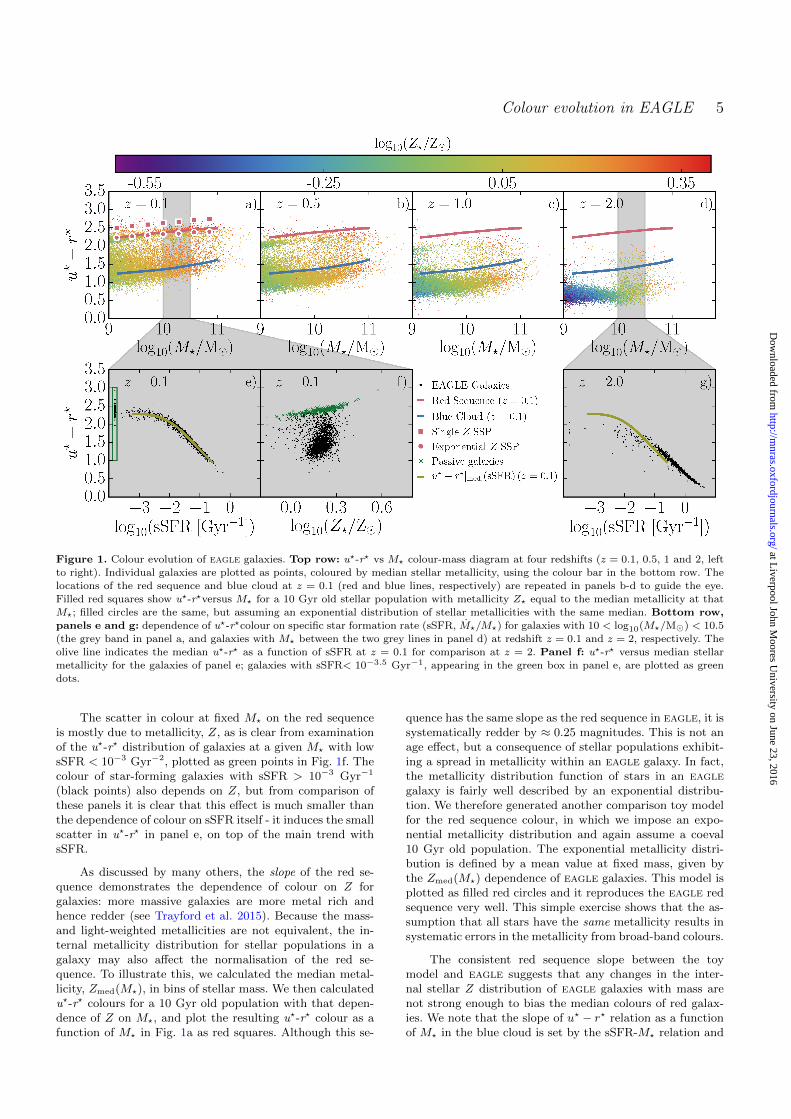
Figure 1a shows that a scatter plot of eagle galaxies in acolour-stellar mass diagram, (u?-r?) vs M?, exhibits strongbimodality in colour at redshift z ≈ 0. The well defined redsequence resides at u?-r?& 2.2 with colours becoming redderwith increasing M?. The blue cloud is at u? − r? ≈ 1.3,with a slope similar to that of the red sequence. These twosequences are indicated by red and blue lines to guide theeye, respectively, obtained by a spline fit to the maxima inthe probability distribution of u?-r? in bins of M?. We keepthe location of these lines fixed in Fig. 1b-d to facilitatecomparison at higher z. We clearly see that:

(i) The red sequence becomes bluer and less populatedwith increasing z. It is in place at z ≈ 1 but has mostlydisappeared by z ≈ 2. A gap in the red sequence is notice-able at z ≈ 1 for M? ∼ 109.7 M�.(ii) The blue sequence becomes bluer with increasing z, andexhibits decreasing scatter.

The main features of the galaxy population thatdrive these trends are illustrated in the bottom panelsof the figure. Figs. 1e & g show that for a narrow stel-lar mass range around M? = 1010.25 M� that u?-r? isstrongly anti-correlated with the specific star formationrate, sSFR ≡ M?/M?, provided the galaxy is star-forming(log10(sSFR/Gyr) & −2). This is not surprising since thelight in the u? filter is dominated by emission from mas-sive and hence young stars, while r? is dominated by theolder population. Galaxies in this plot follow a very tightrelation at a given z, sliding along a narrow locus in colourthat becomes bluer at higher z. At z = 2, the galaxies fol-low almost the same relation in u?-r? versus sSFR as atz = 0, with just a small but noticeable offset towards red-der colours (≈ 0.1 mag) for log10(sSFR/Gyr) & −1.25. Thisis a result of the redder population being younger on av-erage and hence brighter for a z = 2 star-forming galaxy,compared to a star-forming galaxy at z = 0. For lower starformation rates (log10(sSFR/Gyr) . −1.25) the old popu-lation has more influence on u?-r?, and the younger averagestellar age of z = 2 galaxies causes an offset to blue colours.

With u?-r? colour so strongly correlated with sSFR, thecolour vs M? diagram of Fig. 1 is one view of the ‘fun-damental plane of star-forming galaxies’, discussed recentlyby Lagos et al. (2015a). These authors showed that eaglegalaxies from different redshifts fall onto a single 2D surfacewhen plotted in the 3D space of M?−M? and gas fraction (ormetallicity), which they attributed to self-regulation of starformation. Lagos et al. (2015a) also showed that observedgalaxies follow very similar trends. The increasingly bluercolours of the blue cloud towards higher z is a consequenceof the increased star formation activity at fixed M?.

at Liverpool John M



Dow

nloaded from



Figure 1. Colour evolution of eagle galaxies. Top row: u?-r? vs M? colour-mass diagram at four redshifts (z = 0.1, 0.5, 1 and 2, leftto right). Individual galaxies are plotted as points, coloured by median stellar metallicity, using the colour bar in the bottom row. The

locations of the red sequence and blue cloud at z = 0.1 (red and blue lines, respectively) are repeated in panels b-d to guide the eye.

Filled red squares show u?-r?versus M? for a 10 Gyr old stellar population with metallicity Z? equal to the median metallicity at thatM?; filled circles are the same, but assuming an exponential distribution of stellar metallicities with the same median. Bottom row,

panels e and g: dependence of u?-r?colour on specific star formation rate (sSFR, M?/M?) for galaxies with 10 < log10(M?/M�) < 10.5

(the grey band in panel a, and galaxies with M? between the two grey lines in panel d) at redshift z = 0.1 and z = 2, respectively. Theolive line indicates the median u?-r? as a function of sSFR at z = 0.1 for comparison at z = 2. Panel f: u?-r? versus median stellar

metallicity for the galaxies of panel e; galaxies with sSFR< 10−3.5 Gyr−1, appearing in the green box in panel e, are plotted as greendots.

The scatter in colour at fixed M? on the red sequenceis mostly due to metallicity, Z, as is clear from examinationof the u?-r? distribution of galaxies at a given M? with lowsSFR < 10−3 Gyr−2, plotted as green points in Fig. 1f. Thecolour of star-forming galaxies with sSFR > 10−3 Gyr−1

(black points) also depends on Z, but from comparison ofthese panels it is clear that this effect is much smaller thanthe dependence of colour on sSFR itself - it induces the smallscatter in u?-r? in panel e, on top of the main trend withsSFR.

As discussed by many others, the slope of the red se-quence demonstrates the dependence of colour on Z forgalaxies: more massive galaxies are more metal rich andhence redder (see Trayford et al. 2015). Because the mass-and light-weighted metallicities are not equivalent, the in-ternal metallicity distribution for stellar populations in agalaxy may also affect the normalisation of the red se-quence. To illustrate this, we calculated the median metal-licity, Zmed(M?), in bins of stellar mass. We then calculatedu?-r? colours for a 10 Gyr old population with that depen-dence of Z on M?, and plot the resulting u?-r? colour as afunction of M? in Fig. 1a as red squares. Although this se-

quence has the same slope as the red sequence in eagle, it issystematically redder by ≈ 0.25 magnitudes. This is not anage effect, but a consequence of stellar populations exhibit-ing a spread in metallicity within an eagle galaxy. In fact,the metallicity distribution function of stars in an eaglegalaxy is fairly well described by an exponential distribu-tion. We therefore generated another comparison toy modelfor the red sequence colour, in which we impose an expo-nential metallicity distribution and again assume a coeval10 Gyr old population. The exponential metallicity distri-bution is defined by a mean value at fixed mass, given bythe Zmed(M?) dependence of eagle galaxies. This model isplotted as filled red circles and it reproduces the eagle redsequence very well. This simple exercise shows that the as-sumption that all stars have the same metallicity results insystematic errors in the metallicity from broad-band colours.

The consistent red sequence slope between the toymodel and eagle suggests that any changes in the inter-nal stellar Z distribution of eagle galaxies with mass arenot strong enough to bias the median colours of red galax-ies. We note that the slope of u? − r? relation as a functionof M? in the blue cloud is set by the sSFR-M? relation and

at Liverpool John M



Dow

nloaded from



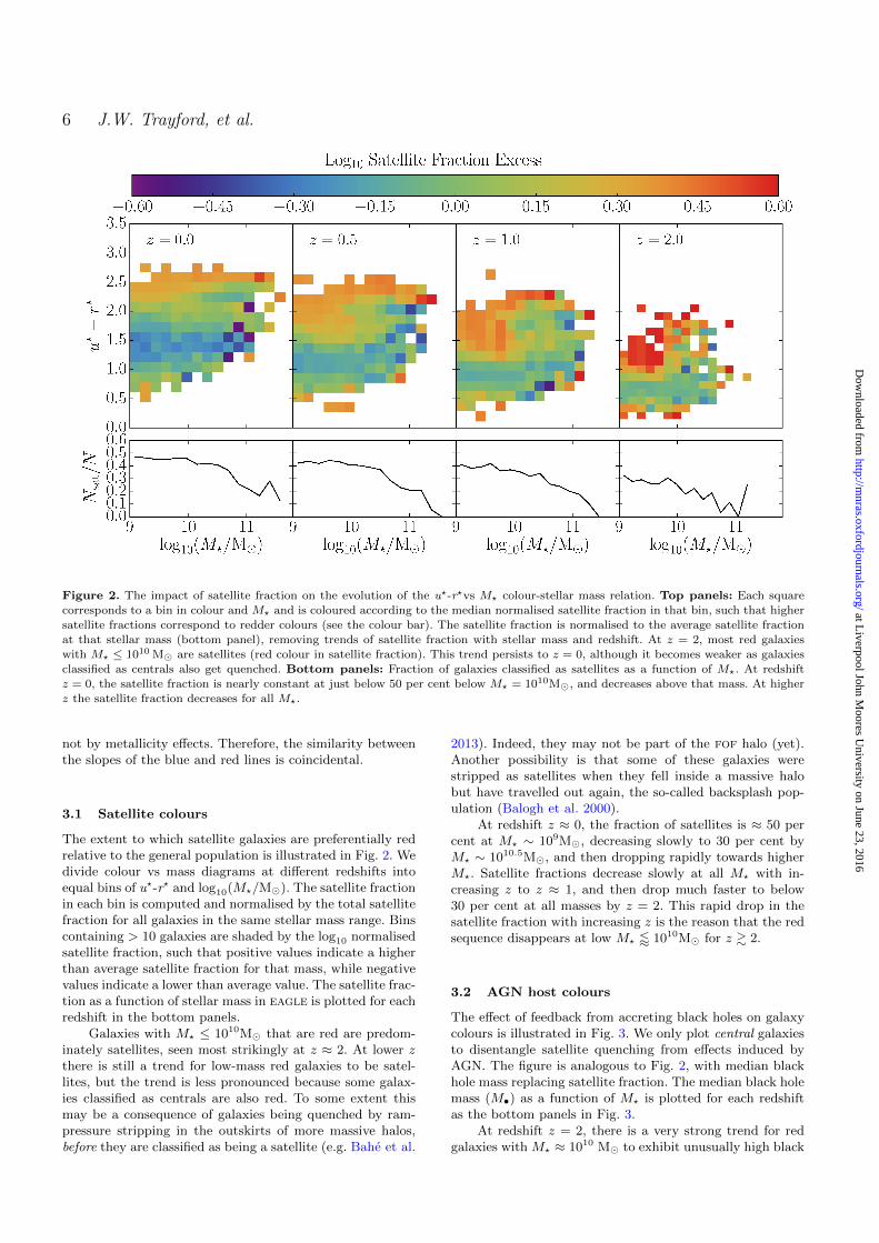
Figure 2. The impact of satellite fraction on the evolution of the u?-r?vs M? colour-stellar mass relation. Top panels: Each squarecorresponds to a bin in colour and M? and is coloured according to the median normalised satellite fraction in that bin, such that higher

satellite fractions correspond to redder colours (see the colour bar). The satellite fraction is normalised to the average satellite fraction

at that stellar mass (bottom panel), removing trends of satellite fraction with stellar mass and redshift. At z = 2, most red galaxieswith M? ≤ 1010 M� are satellites (red colour in satellite fraction). This trend persists to z = 0, although it becomes weaker as galaxies

classified as centrals also get quenched. Bottom panels: Fraction of galaxies classified as satellites as a function of M?. At redshift

z = 0, the satellite fraction is nearly constant at just below 50 per cent below M? = 1010M�, and decreases above that mass. At higherz the satellite fraction decreases for all M?.

not by metallicity effects. Therefore, the similarity betweenthe slopes of the blue and red lines is coincidental.

3.1 Satellite colours

The extent to which satellite galaxies are preferentially redrelative to the general population is illustrated in Fig. 2. Wedivide colour vs mass diagrams at different redshifts intoequal bins of u?-r? and log10(M?/M�). The satellite fractionin each bin is computed and normalised by the total satellitefraction for all galaxies in the same stellar mass range. Binscontaining > 10 galaxies are shaded by the log10 normalisedsatellite fraction, such that positive values indicate a higherthan average satellite fraction for that mass, while negativevalues indicate a lower than average value. The satellite frac-tion as a function of stellar mass in eagle is plotted for eachredshift in the bottom panels.

Galaxies with M? ≤ 1010M� that are red are predom-inately satellites, seen most strikingly at z ≈ 2. At lower zthere is still a trend for low-mass red galaxies to be satel-lites, but the trend is less pronounced because some galax-ies classified as centrals are also red. To some extent thismay be a consequence of galaxies being quenched by ram-pressure stripping in the outskirts of more massive halos,before they are classified as being a satellite (e.g. Bahe et al.

2013). Indeed, they may not be part of the fof halo (yet).Another possibility is that some of these galaxies werestripped as satellites when they fell inside a massive halobut have travelled out again, the so-called backsplash pop-ulation (Balogh et al. 2000).

At redshift z ≈ 0, the fraction of satellites is ≈ 50 percent at M? ∼ 109M�, decreasing slowly to 30 per cent byM? ∼ 1010.5M�, and then dropping rapidly towards higherM?. Satellite fractions decrease slowly at all M? with in-creasing z to z ≈ 1, and then drop much faster to below30 per cent at all masses by z = 2. This rapid drop in thesatellite fraction with increasing z is the reason that the redsequence disappears at low M? / 1010M� for z & 2.

3.2 AGN host colours

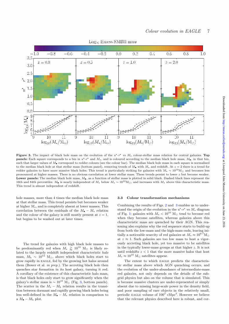
The effect of feedback from accreting black holes on galaxycolours is illustrated in Fig. 3. We only plot central galaxiesto disentangle satellite quenching from effects induced byAGN. The figure is analogous to Fig. 2, with median blackhole mass replacing satellite fraction. The median black holemass (M•) as a function of M? is plotted for each redshiftas the bottom panels in Fig. 3.

At redshift z = 2, there is a very strong trend for redgalaxies with M? ≈ 1010 M� to exhibit unusually high black

at Liverpool John M



Dow

nloaded from



Figure 3. The impact of black hole mass on the evolution of the u?-r? vs M? colour-stellar mass relation for central galaxies. Toppanels: Each square corresponds to a bin in u?-r? and M?, and is coloured according to the median black hole mass, M•, in that bin,

such that larger values of M• correspond to redder colours (see the colour bar). The median black hole mass in each square is normalised

to the median black hole at that stellar mass (bottom panel), removing trends of M• with M? and redshift. At z = 2 there is a trend forredder galaxies to have more massive black holes. This trend is particularly striking for galaxies with M? ∼ 1010M� and becomes less

pronounced at higher masses. There is no obvious correlation at lower stellar mass. These trends persist to lower z but become weaker.

Lower panels: The median black hole mass, M•, as a function of stellar mass is plotted in solid black. Dashed black lines represent the16th and 84th percentiles. M• is nearly independent of M? below M? ∼ 1010M�, and increases with M? above this characteristic mass.

This trend is almost independent of redshift.

hole masses, more than 4 times the median black hole massat that stellar mass. This trend persists but becomes weakerat higher M?, and is completely absent at lower masses. Thiscorrelation between the residuals of the M• −M? relationand the colour of the galaxy is still mostly present at z = 1,but begins to be washed out at later times.

The trend for galaxies with high black hole masses tobe predominantly red when M? ' 1010 M� is likely re-lated to the largely redshift independent characteristic halomass, Mh ∼ 1012 M�, above which black holes start togrow rapidly in eagle, fed by the growing hot halos aroundthem (Bower et al. in prep.). The accreting black hole thenquenches star formation in its host galaxy, turning it red.A corollary of the existence of this characteristic halo mass,is that black holes only start to grow significantly when thegalaxy’s stellar mass is ∼ 1010 M� (Fig. 3, bottom panels).The scatter in the M? −Mh relation results in the transi-tion between dormant and rapidly growing black holes beingless well-defined in the M• −M? relation in comparison toa M• −Mh plot.

3.3 Colour transformation mechanisms

Combining the results of Figs. 2 and 3 enables us to under-stand the origin of the evolution in the u?-r? vs M? diagramof Fig. 1: galaxies with M? < 1010 M� tend to become redwhen they become satellites, whereas galaxies above thischaracteristic mass are quenched by their AGN. This rea-soning also explains why the red sequence starts to build-upfrom both the low-mass and the high-mass ends, leaving ini-tially a noticeable scarcity of red galaxies at M? ≈ 109.7M�at z ≈ 1. Such galaxies are too low mass to host a vigor-ously accreting black hole, yet too massive to be satellitesin the typically lower-mass groups at that higher z. It is notuntil redshifts z < 1 that the more massive halos that hostM? ≈ 1010 M� satellites appear.

The extent to which eagle predicts the characteris-tic stellar mass above which AGN quenching occurs, andthe evolution of the under-abundance of intermediate-massred galaxies, not only depends on the details of the sub-grid physics but also on the volume that is simulated. Thisis because massive clusters are under-represented or simplyabsent due to missing large-scale power in the density field,and poor sampling of rare objects in the relatively small,periodic eagle volume of 1003 cMpc3. However we believethat the relevant physics described here is robust, and cor-

at Liverpool John M



Dow

nloaded from



roborates the similar conclusions of Gabor & Dave (2012)who used an ad-hoc model for quenching in massive galax-ies, as opposed to our physically motivated subgrid schemefor the eagle simulations that are implemented on smaller(sub-kpc) scales.

A corollary of satellite quenching for lower-mass galax-ies, and AGN quenching for more massive galaxies, is thatthese low- and high-mass red galaxies tend to inhabit thesame dark matter halos. The more massive red galaxy isthe central galaxy of this halo and is quenched by its AGN.Conversely, the lower-mass red galaxies are the satellites ofa massive central red galaxy. As a consequence, the low-and high-mass red galaxies have similar clustering strengths,with both clustering more strongly than blue galaxies. ea-gle reproduces the observed clustering as a function ofcolour and luminosity well, as will be discussed by Artaleet al. (in prep.). We next investigate how, and at what rate,individual galaxies move through the u?-r? vs M? diagram.

4 COLOUR EVOLUTION OF INDIVIDUALGALAXIES

4.1 The flow of galaxies in the colour-M? plane

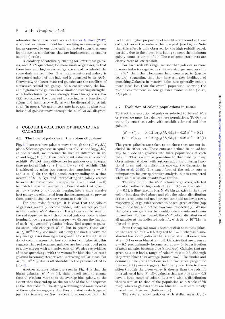
Fig. 4 illustrates how galaxies move through the (u?-r?, M?)plane. Selecting galaxies in equal bins of u?-r? and log10(M?)at one redshift, we measure the median difference in u?-r? and log10(M?) for their descendant galaxies at a secondredshift. We plot these differences for galaxies over an equaltime period at high (z ≈ 1) and low (z ≈ 0) redshift. Thisis achieved by using two consecutive snapshots (z = 1.3and z = 1) for the right panel, corresponding to a timeinterval of ≈ 0.9 Gyr, and interpolating the galaxy vectorsbetween the lowest redshift snapshots (z = 0.1 and z = 0)to match the same time period. Descendants that grow inM? by a factor > 4 through merging into a more massivehost galaxy are eliminated from the measurement, to preventthem contributing extreme vectors to their bin.

For both redshift ranges, it is clear that the coloursof galaxies generally become redder, with vectors pointingin the positive u?-r? direction. Exceptions can be seen onthe red sequence, in which some red galaxies become star-forming following a gas-rich merger - we discuss the fractionof such ‘rejuvenated’ galaxies below. Red sequence galax-ies show little change in u?-r?, but in general those withM? . 1010.75M� lose mass, with only the most massive redsequence galaxies showing mass growth. Considering that wedo not count mergers into hosts of factor > 4 higher M?, thissuggests that red sequence galaxies are being stripped priorto a dry merger with a massive central. We also see evidenceof ‘mass quenching’, with the vectors for blue-cloud selectedgalaxies becoming steeper with increasing stellar mass. ForM? > 1010M� this is attributable to the presence of AGN(Fig. 3).

Another notable behaviour seen in Fig. 4 is that thebluest galaxies (u?-r? ≈ 0.5, right panel) tend to changetheir u?-r?colour more than the average blue galaxy, to theextent that they end-up on the red side of the blue sequenceat the later redshift. The strong reddening and mass increaseof these galaxies suggests that they are starbursts triggeredjust prior to a merger. Such a scenario is consistent with the

fact that a higher proportion of satellites are found at thesecolours than at the centre of the blue peak (see Fig. 2). Notethat this effect is only observed for the high redshift panel,partially due to the bluest bins failing to meet the minimumgalaxy count criterion of 10. These extreme starbursts areclearly rarer at low redshift.

For each redshift range, we see that galaxies in moremassive halos (orange vectors) have a stronger median shiftin u?-r? than their low-mass halo counterparts (purplevectors), suggesting that they have a higher likelihood ofquenching.Galaxies in massive halos also generally exhibitmore mass loss than the overall population, showing therole of environment in how galaxies evolve in the (u?-r?,M?) plane.

4.2 Evolution of colour populations in eagle

To track the evolution of galaxies selected to be red, blueor green, we must first define these populations. To do thiswe apply cuts that evolve with redshift z for red and bluegalaxies.

(u? − r?)red > 0.2 log10(M?/M�) − 0.25 z0.6 + 0.24

(u? − r?)blue < 0.2 log10(M?/M�) − 0.25 z0.6 − 0.3(1)

The green galaxies are taken to be those that are not in-cluded in either set. These cuts are defined in an ad-hocway to divide the galaxies into three populations at eachredshift. This is a similar procedure to that used by manyobservational studies, with authors adopting differing func-tional forms and normalisations (see e.g. the discussion inTaylor et al. 2015). The exact form of the colour cuts isunimportant for our qualitative analysis, but is consideredwhen we discuss our quantitative results.

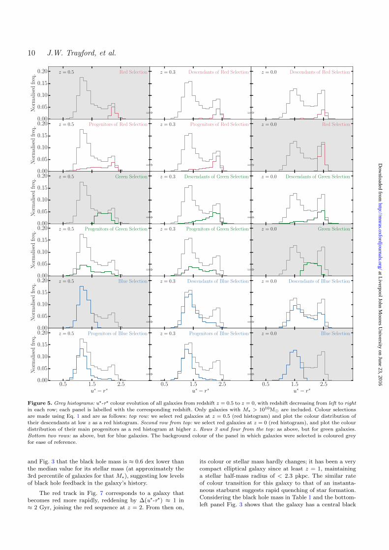
The evolution of the u?-r? colours of galaxies, selectedby colour either at high redshift (z = 0.5) or low redshift(z = 0.1), is illustrated in Fig. 5. We bin galaxies in the threecolour bins described above and plot the colour distributionof the descendants and main progenitors (odd and even rows,respectively) of galaxies selected to be red, green or blue (toptwo, middle two, and bottom two rows, respectively). We usethe galaxy merger trees to identify descendants and mainprogenitors. For each panel, the u?-r? colour distribution ofall galaxies at the indicated redshift, with M? > 1010M�, isplotted in grey.

From the top two rows it becomes clear that most galax-ies that are red at z = 0.5 stay red to z = 0, whereas a sub-stantial fraction of galaxies that are red at z = 0 were greenat z = 0.1 or even blue at z = 0.5. Galaxies that are green atz = 0.5 predominantly become red at z = 0, but a fractionof green galaxies becomes blue (third row). Galaxies that aregreen at z = 0 had a range of colours at z = 0.5, althoughthey were bluer than average (fourth row). The similar anddominant blue (red) fractions in the two green progenitor(descendant) panels suggests that the typical time to tran-sition through the green valley is shorter than the redshiftintervals used here. Finally, galaxies that are blue at z = 0.5have a large range of colours at z = 0 with a distributionthat is similar to that of the population as a whole (fifthrow), whereas galaxies that are blue at z = 0 were mostlyblue at z = 0.5 as well (bottom row).

The rate at which galaxies with stellar mass M? >

at Liverpool John M



Dow

nloaded from



9.5 10.0 10.5 11.0log10(M?/M�)

z = 1.0

9.5 10.0 10.5 11.0log10(M?/M�)

0.0

0.5

1.0

1.5

2.0

2.5

3.0

u?−r?

z = 0.0

All

M200, crit < 1013 M�M200, crit > 1013 M�

Figure 4. The flow of galaxies in (u?-r?, M?) space between two redshifts, z1 to z2. Right panel shows the galaxy flow between z1 = 1.3and z2 = 1 snapshots, a period of ≈ 0.9 Gyr. The left panel shows the galaxy flow interpolated between the z = 0.1 and z = 0 snapshots

to yield the same time period, with z1 = 0.07 and z2 = 0. Black circles represent the mean location of galaxies at z1, selected in a bin of

u?-r?- M?; the size of the circle is proportional to the logarithm of the total stellar mass in galaxies in that bin. Black vectors representthe mean motion of the galaxies in that bin between z1 and z2. Orange vectors (purple vectors) are for those galaxies that at redshift

z2 belong to halos with virial mass M200, crit > 1013M� (M200, crit < 1013M�). Centre coordinates and vectors sampling fewer than 10

galaxies are not plotted. The overall distribution at the later redshift is plotted as grey contours for comparison. We do not take intoaccount galaxies merging into hosts that are more than four times their mass, illustrating such mergers in more detail in Fig. 8.

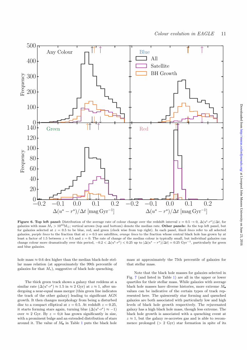
1010M� at z = 0.5 change u?-r? colour over the redshiftrange z = 0.5 to z = 0 (elapsed time ∆t ≈ 5 Gyr) is quan-tified in Fig. 6. We identify the z = 0 descendant for allgalaxies with M? > 1010M� at z = 0.5, compute the changein colour, ∆(u?-r?), and plot a histogram of rates, ∆(u?-r?)/∆t. We also identify if a galaxy is a satellite at z = 0.5,or if the mass of its central black hole increases by a factor≥ 1.5. This threshold is chosen to represent an above av-erage black hole growth, while still providing a significantsample of galaxies.

The rate of change of the median colour of galaxiesis small, ∆(u?-r?)/∆t ≈ 0.08 mag Gyr−1 to the red, butis larger for galaxies whose black hole grows more thanaverage (∆(u?-r?)/∆t ≈ 0.09 mag Gyr−1) or those thatare satellites (∆(u?-r?)/∆t ≈ 0.12 mag Gyr−1). Galaxiesthat are red at z = 0.5 typically change little in colour toz = 0, (∆(u?-r?)/∆t ≈ 0.03 mag Gyr−1), except for theoccasional outlier that becomes blue. The rate of change ofthe median colour is larger for galaxies that are green orblue at z = 0.5, with individual galaxies changing colourmore rapidly, both to the red and to the blue. Galaxiesthat are satellites can undergo rapid changes to the red,∆(u?-r?)/∆t & 0.2 mag Gyr−1, whether blue or green atz = 0.5. Note that this rate is averaged over a considerableperiod (≈ 5 Gyr), and instantaneous rates of colour changefor galaxies can be much higher, as explored below.

4.3 Colour-mass tracks of individual galaxies

We have examined a large number of tracks of individ-ual galaxies in (u?-r?, M?) space and have identified three

Table 1. Properties of the galaxies plotted as main tracks in

Figs. 7-8. The Symbol/Figure is given to identify the galax-ies on the figures. For each galaxy we quote the unique galaxy

identifier (GalaxyID) taken from the eagle public database

(McAlpine et al. 2015), the z = 0 black hole mass (M•), andindicate whether a galaxy was ever classified as a satellite (y) or

not (n).

Sym./Fig. GalaxyID M•/M� Satellite

Circle/7 18169630 7.09× 106 nSquare/7 15829793 1.03× 108 n

Triangle/7 14096270 6.00× 107 n

Circle/8 15197399 1.84× 108 y

generic tracks of central galaxies that we illustrate in Fig. 7.In Fig. 8 we also show the track of a central galaxy that isvery massive at z = 0 (M? ∼ 1011M�), to illustrate indi-vidual tracks of satellites that merge with it. More detailsof the four galaxies tracked in these panels are given in Ta-ble 1. The time-scale over which galaxies transition to thered sequence is compared to that of a passively evolvingpopulation, by plotting (single) star-burst tracks initiatedat different times (grey curves in middle panels).

The blue track in Fig. 7 is for a galaxy that remainsin the blue cloud down to z = 0, forming stars in a bluedisc that grows in time. As its sSFR decreases with time,and the contribution of an older population of stars becomesmore important, it slowly reddens, with ∆(u?-r?) ≈ 0.2 fromz = 1 to z = 0 (elapsed time ≈ 8 Gyr). We see from Table 1

at Liverpool John M



Dow

nloaded from



0.00

0.05

0.10

0.15

0.20

Nor

mal

ised

freq. Red Selectionz = 0.5 Descendants of Red Selectionz = 0.3

=⇒

Descendants of Red Selectionz = 0.0

=⇒

0.5 1.5 2.5u∗ − r∗

0.00

0.05

0.10

0.15

0.20

Nor

mal

ised

freq. Progenitors of Red Selectionz = 0.5

0.5 1.5 2.5u∗ − r∗

Progenitors of Red Selectionz = 0.3

=⇒

0.5 1.5 2.5u∗ − r∗

Red Selectionz = 0.0

=⇒

0.00

0.05

0.10

0.15

0.20

Nor

mal

ised

freq. Green Selectionz = 0.5 Descendants of Green Selectionz = 0.3

=⇒

Descendants of Green Selectionz = 0.0

=⇒

0.5 1.5 2.5u∗ − r∗

0.00

0.05

0.10

0.15

0.20

Nor

mal

ised

freq. Progenitors of Green Selectionz = 0.5

0.5 1.5 2.5u∗ − r∗

Progenitors of Green Selectionz = 0.3

=⇒

0.5 1.5 2.5u∗ − r∗

Green Selectionz = 0.0

=⇒

0.00

0.05

0.10

0.15

0.20

Nor

mal

ised

freq. Blue Selectionz = 0.5 Descendants of Blue Selectionz = 0.3

=⇒

Descendants of Blue Selectionz = 0.0

=⇒

0.5 1.5 2.5u∗ − r∗

0.00

0.05

0.10

0.15

0.20

Nor

mal

ised

freq. Progenitors of Blue Selectionz = 0.5

0.5 1.5 2.5u∗ − r∗

Progenitors of Blue Selectionz = 0.3

=⇒

0.5 1.5 2.5u∗ − r∗

Blue Selectionz = 0.0

=⇒

Figure 5. Grey histograms: u?-r? colour evolution of all galaxies from redshift z = 0.5 to z = 0, with redshift decreasing from left to right

in each row; each panel is labelled with the corresponding redshift. Only galaxies with M? > 1010M� are included. Colour selectionsare made using Eq. 1 and are as follows: top row: we select red galaxies at z = 0.5 (red histogram) and plot the colour distribution oftheir descendants at low z as a red histogram. Second row from top: we select red galaxies at z = 0 (red histogram), and plot the colour

distribution of their main progenitors as a red histogram at higher z. Rows 3 and four from the top: as above, but for green galaxies.Bottom two rows: as above, but for blue galaxies. The background colour of the panel in which galaxies were selected is coloured grey

for ease of reference.

and Fig. 3 that the black hole mass is ≈ 0.6 dex lower thanthe median value for its stellar mass (at approximately the3rd percentile of galaxies for that M?), suggesting low levelsof black hole feedback in the galaxy’s history.

The red track in Fig. 7 corresponds to a galaxy thatbecomes red more rapidly, reddening by ∆(u?-r?) ≈ 1 in≈ 2 Gyr, joining the red sequence at z = 2. From then on,

its colour or stellar mass hardly changes; it has been a verycompact elliptical galaxy since at least z = 1, maintaininga stellar half-mass radius of < 2.3 pkpc. The similar rateof colour transition for this galaxy to that of an instanta-neous starburst suggests rapid quenching of star formation.Considering the black hole mass in Table 1 and the bottom-left panel Fig. 3 shows that the galaxy has a central black

at Liverpool John M



Dow

nloaded from



0

100

200

300

400

500

Fre

qu

ency

Any Colour BlueAll

Satellite

BH Growth

−0.2 −0.1 0.0 0.1 0.2∆(u? − r?)/∆t [mag Gyr−1]

0

20

40

60

80

100

120

140

Fre

qu

ency

Green

−0.2 −0.1 0.0 0.1 0.2∆(u? − r?)/∆t [mag Gyr−1]

Red

Figure 6. Top left panel: Distribution of the average rate of colour change over the redshift interval z = 0.5 → 0, ∆(u?-r?)/∆t, for

galaxies with mass M? > 1010M�; vertical arrows (top and bottom) denote the median rate. Other panels: As the top left panel, butfor galaxies selected at z = 0.5 to be blue, red, and green (clock wise from top right). In each panel, black lines refer to all selected

galaxies, purple lines to the fraction that at z = 0.5 are satellites, orange lines to the fraction whose central black hole has grown by at

least a factor of 1.5 between z = 0.5 and z = 0. The rate of change of the median colour is typically small, but individual galaxies canchange colour more dramatically over this period, −0.2 < ∆(u?-r?) < 0.25 up to |∆(u? − r?)/∆t| = 0.25 Gyr−1, particularly for green

and blue galaxies.

hole mass ≈ 0.6 dex higher than the median black-hole stel-lar mass relation (at approximately the 99th percentile ofgalaxies for that M?), suggestive of black hole quenching.

The thick green track shows a galaxy that reddens at asimilar rate (∆(u?-r?) ≈ 1.5 in ≈ 2 Gyr) at z ≈ 1, after un-dergoing a near-equal mass merger (thin green line indicatesthe track of the other galaxy) leading to significant AGNgrowth. It then changes morphology from being a disturbeddisc to a compact elliptical at z = 0.5. At redshift z = 0.25,it starts forming stars again, turning blue (∆(u?-r?) ≈ −1)over ≈ 2 Gyr. By z = 0,it has grown significantly in size,with a prominent bulge and an extended distribution of starsaround it. The value of M• in Table 1 puts the black hole

mass at approximately the 75th percentile of galaxies forthat stellar mass.

Note that the black hole masses for galaxies selected inFig. 7 (and listed in Table 1) are all in the upper or lowerquartiles for their stellar mass. While galaxies with averageblack hole masses have diverse histories, more extreme M•values can be indicative of the certain types of track rep-resented here. The quiescently star forming and quenchedgalaxies are both associated with particularly low and highlevels of black hole growth respectively. The rejuvenatedgalaxy has a high black hole mass, though less extreme. Theblack hole growth is associated with a quenching event atz ≈ 1, but the galaxy re-accretes gas and is able to recom-mence prolonged (> 2 Gyr) star formation in spite of its

at Liverpool John M



Dow

nloaded from



9.0 9.5 10.0 10.5 11.0log10(M?/M�)

0.0

0.5

1.0

1.5

2.0

2.5

3.0

u∗ −

r∗

2 4 6 8 10 12 14t [Gyr]

4.0 2.0 1.0 0.5 0.25 0.1 0.0z

z = 1.0 z = 0.5 z = 0.0

z = 1.0 z = 0.5 z = 0.0

z = 1.0 z = 0.5 z = 0.0

4.0 2.0 1.0 0.5 0.25 0.1 0.0z

4.0 2.0 1.0 0.5 0.25 0.1 0.0z

Figure 7. Tracks illustrating the change in mass, colour and morphology, of a quiescently star-forming galaxy (thick blue curve & filled

circles), a rapidly quenched galaxy (thick red curve & filled triangles), and a rejuvenated galaxy (thick green curve & filled squares). Thintracks show merging satellites (see caption of Fig. 8). Left and middle panels: tracks in the (u?-r?, M?) plane (left panel) and colour as

function of time and redshift (middle panel), from redshift z = 4 to z = 0. Symbol colour corresponds to cosmic time as per the colour

bar. Background contours in the left panel correspond to the z = 0 colour-M? distribution. Grey tracks in the middle panel depict thecolour evolution of a passively-evolving coeval starburst (indicated with an arrow). Each burst is assumed to be composed of stars with

an exponential distribution of metallicities with given mean. The width of the grey region corresponds to varying this mean metallicity

over the range of [1/3,3] times solar (Z� = 0.0127). Right panel: edge-on gri-composite image of side length 40 pkpc, calculated usingray-tracing to account for dust (Trayford et al. 2015, in prep.), for the z = 0 galaxy and its z = 0.5 and z = 1 main progenitor. The

corresponding symbol for each track is indicated on galaxy images.

9.0 9.5 10.0 10.5 11.0log10(M?/M�)

0.0

0.5

1.0

1.5

2.0

2.5

3.0

u∗ −

r∗

2 4 6 8 10 12 14t [Gyr]

Central

Satellite

4.0 2.0 1.0 0.5 0.25 0.1 0.0z

z = 1.5 z = 1.0 z = 0.7

z = 0.5 z = 0.4 z = 0.3

z = 0.2 z = 0.1 z = 0.0

Figure 8. Same as Fig. 7, but for a massive galaxy (green track & filled circles) and galaxies that merge with it (thin tracks). Tracksfor merging galaxies (merging with M? > 109 M�) are coloured purple when they are centrals, and orange when they are satellites as

indicated in the legend; a star identifies the last snapshot before the satellite merges with the massive galaxy, and the track is linked to

that of the massive galaxy at the following snapshot by a dashed line. The right panel shows edge-on gri-composite images of the centralgalaxy of side length 40 pkpc, at various redshifts labelled in each separate panel.

high black hole mass. We saw in Fig. 3 that for z = 0 and atthese masses the overall correlation between galaxy colourand the residuals of the M•-M? relation is rather weak.

The massive z = 0 galaxy in Fig. 8 is a blue star-forming disc until just below z = 1, after which it becomesred and evolves into an elongated elliptical. Thin lines show

the tracks of five galaxies that merge with it, with the linecolour changing from purple to orange while these galaxiesbecome satellites. Examination of these tracks reveals thatwhile some galaxies become red when they are still centrals,most galaxies quench after being identified as satellites. Thissuggests that satellite identification is a good predictor of

at Liverpool John M



Dow

nloaded from



0.0 0.5 1.0 1.5 2.0 2.5 3.0 3.5

u −r0

50

100

150

200

250

300

Fre

quen

cy

AllQuiescently SFRapidly Reddened

Figure 9. u?-r? colour distribution for M? > 1010M� galaxies at

z = 0. Galaxies identified as ‘quiescently star-forming ’are plotted

in purple, while those that underwent a rapid colour transitionto the red are plotted in orange. The combined distribution is

plotted in black. We see that the quiescently star-forming galax-

ies predominately inhabit the present-day blue cloud, but witha tail to red colours. Galaxies that underwent a rapid reddening

(∆(u?-r?) > 0.8 in 2 Gyr) are predominately red at z = 0, but the

distribution has a blue tail resulting from recent star formation.

colour change in eagle, particularly for galaxies falling intoa more massive halo. The satellite tracks exhibit a character-istic shape of rapid quenching followed by stellar mass loss,as the galaxy is stripped and eventually merges. We alsosee that the central galaxy exhibits quite a stochastic colourevolution compared to those in Fig. 7. This is perhaps dueto the higher frequency of satellite interactions and mergersfor the higher mass halo represented in Fig. 8, with onlythe rejuvenated track of Fig. 7 showing (two) mergers withsatellites of M? > 109M�.

The heterogeneous colour evolution of galaxies il-lustrated in Fig. 7 and 8 are consistent with observa-tions that the green valley population is diverse (e.g.Cortese & Hughes 2009; Schawinski et al. 2014). In particu-lar, Cortese & Hughes (2009) also find examples of galaxiesmoving off the red sequence through re-accretion of gas rem-iniscent of the green track in Fig. 7.

To quantify the fraction of galaxies that undergo a rapidcolour transformation, we trace the main progenitors of allgalaxies with mass M? > 1010M� at z = 0 back in time(a sample of ≈ 3000 galaxies). We find that the fraction ofgalaxies with at least one ∆(u?-r?) > 0.8 change over any2 Gyr period in their history is ≈ 40 per cent. We will refer tosuch galaxies as rapidly reddening galaxies; they tend to fol-low a track similar to the red track in Fig.7. Of the galaxiesthat redden quickly, ≈ 1.6 per cent undergo a colour changeto the blue of ∆(u?-r?) < −0.8 over a 2 Gyr period. We willrefer to this small fraction of galaxies as ‘rejuvenated’; they

0 2 4 6 8 10 12 14t [Gyr]

0

10

20

30

40

50

60

70

80

90

Fre

quen

cy

1010 < M∗(z = 0)/M� < 1010.5

All

Satellites

BH growth

0 2 4 6 8 10 12 14t [Gyr]

0

10

20

30

40

50

Fre

quen

cy

1010.5 < M∗(z = 0)/M� < 1011

All

Satellites

BH growth

Figure 10. Histograms of the time interval galaxies spent cross-

ing the green valley from being blue to becoming red, ∆tgreen(see text). The black histogram is for all galaxies in the current

mass selection, purple histogram for galaxies that are satellites

at z = 0, orange histogram for galaxies whose black holes grewby more than a factor of 1.5 while crossing the green valley. Me-

dian values for the selections are plotted as dashed lines with the

corresponding colour. Top panel shows galaxies selected in thez = 0 mass range 1010 < M?/M� < 1010.5, with the bottom

panel corresponding to 1010.5 < M?/M� < 1011. Satellite galax-

ies dominate in both mass ranges. The transition time-scale for ablue galaxy to turn red is typically . 2 Gyr, which corresponds

to the time a blue population of stars reddens passively, as seen

in Fig.7.

at Liverpool John M



Dow

nloaded from



follow a track similar to the green track in Fig. 72. Galax-ies that do not ever undergo such a rapid reddening eventmake-up 60 per cent of the sample. We will refer to these as‘quiescently star-forming’ galaxies; they follow a track sim-ilar to the blue track in Fig.7.

Fig. 9 shows the distribution of z = 0 colours for 1010 <M?/M� < 1010.5 galaxies classified as having undergone arapid transformation to redder colour (orange histogram),and those that never underwent such a rapid reddening (qui-escently star-forming galaxies, purple histogram). A smallfraction of galaxies become red without ever experiencinga rapid reddening event: this is the tail of the purple his-togram towards red u?-r? colour. Similarly, there is a tailto blue u?-r? colour in the orange histogram, representinggalaxies that underwent a rapid colour transition to the red,followed by more recent star formation turning them blueonce more. The fraction of these galaxies is much higherthan the 1.6 per cent of galaxies we classified as ‘rejuve-nated’: the majority of galaxies that are blue now but werered in the past (≈ 10% of total), became blue more gradu-ally than the ∆(u?-r?) = −0.8 over 2 Gyr that we used todefine ‘rejuvenated galaxies’.

Galaxies must become blue rapidly or traverse the entiregreen valley to meet these criteria. However, it is also inter-esting to note the probability that a galaxy identified in thegreen valley is on a bluer trajectory in the colour-M? plane.We identify this for green valley galaxies at z < 2, enforc-ing that a galaxy must undergo a monotonic colour changeof ∆(u?-r?) < −0.05 to be deemed significant (above thelevel of photometric error, e.g. Padmanabhan et al. 2008).We find that the eagle green valley galaxies have a 17%chance of being on a significantly blue trajectory. Conversely,we find the probability of a green galaxy being on a signifi-cantly red trajectory to be 75%, taking ∆(u?-r?) > 0.05 asthe criteria for being significant.

The tracks of individual galaxies enable us to charac-terise the colour transition time-scale of a galaxy by the timeinterval, ∆tgreen, it spent in the green valley on its way fromthe blue cloud to the red sequence. We calculate ∆tgreenas follows: using Eq. (1) we select red galaxies at z = 0 andtrace their main progenitors back in time to identify the lasttime (t1) they became red and the last time (t2) they wereblue. Histograms of colour transition times, ∆tgreen ≡ t1−t2,for galaxies that at z = 0 have 1010 < M?/M� < 1010.5 and1010.5 < M?/M� < 1011 are plotted in Fig. 10 (top andbottom panels, respectively).

The mode of the colour transition time distribution is≈ 1.5 Gyr, with a median of ≈ 2 Gyr, mostly independentof whether quenching is likely due to becoming a satellite orAGN activity (purple and orange histograms, respectively).This is the time-scale for a passively evolving blue popula-tion of stars to turn red, as can be seen from Fig.7. Strik-ingly, there is a very long tail to high values in the dis-tribution of ∆tgreen as inefficient quenching allows a smallfraction of galaxies to spend a long time in the green val-

2 Galaxies may also undergo slower colour transitions due to sec-

ular evolution, and the number density of galaxies does not re-main constant because of mergers. These quoted fractions there-fore inevitably depend on how galaxies are selected. i.e. the colourchoice we made in Eq. 1.

ley before eventually turning red, whether due to becominga satellite or hosting an AGN. Though quenched galaxiesare more prevalent in high-mass halos, the colour transitiontime-scales show little dependence on halo mass. Despitethis, the longest time-scales we measure are for halo masses< 1013 M�.

The time-scales for colour transition and the quenchingof star formation are clearly linked, however colour transi-tion times are longer due to the passive evolution of stellarpopulations. This is illustrated by the grey curves in Fig. 7and 8, showing that the colour transition time for an SSPis ≈ 2 Gyr. The quenching time-scales of observed satel-lites presented by e.g. Muzzin et al. (2014) and Wetzel et al.(2013) are significantly shorter, typically . 0.5 Gyr and. 0.8 Gyr respectively. Although the u?-r? colour indexalone is not sensitive enough to resolve these quenchingtimes, the typical colour transition times of eagle galax-ies are consistent with such rapid quenching.

However, there are cluster studies in the 0 < z < 0.5redshift range that infer longer timescales (' 1 Gyr, e.g.von der Linden et al. 2010; Vulcani et al. 2010; Haines et al.2013). Fig. 10 does show a tail to longer quenching times forboth AGN and satellites, though they are not typical at lowredshift. Ultimately, the different observational tracers andmodelling used to infer quenching times are still subject tosignificant systematics that may explain the different mea-surements (McGee et al. 2014). In particular, colour transi-tion and quenching timescales are not equivalent, and galax-ies may move between the red and blue populations whenobserved in optical and UV colour (Cortese 2012, e.g.). Ananalysis of the physical quenching timescale and its evolu-tion is left to a future study.

5 CONCLUSIONS

We have investigated the evolution and origin of the coloursof galaxies in the eagle cosmological hydrodynamical simu-lation (Schaye et al. 2015; Crain et al. 2015). We apply thesingle population synthesis models from Bruzual & Charlot(2003) to model galaxy colours in the absence of dust,as described by Trayford et al. (2015). We also use galaxymerger trees to trace descendants as well as main progeni-tors through time.

The u?-r? vs M? diagram is bimodal at redshift z = 0,with a clearly defined red sequence of quenched galaxies, anda blue cloud of star-forming galaxies. The scatter and slopeof the red sequence are both determined mainly by stellarmetallicity, while the normalisation additionally depends onstellar age (Fig. 1). The scatter in the blue cloud, in contrast,is mostly due to scatter in the specific star formation rate atfixed stellar mass (sSFR = M?/M?). The slope of blue cloudcolours versus M? is similar to that of the red sequence, butas their origins are different, this is coincidental. At higherz, both colour sequences become bluer, and the red sequencebecomes less populated until it has mostly disappeared byz = 2.

From studying the evolution of eagle galaxies in u?-r?

and M?, we note that in general:

• Galaxies in eagle turn red either because they becomesatellites (mainly at lower masses, see Fig. 2) or because offeedback from their central supermassive black hole (mainly

at Liverpool John M



Dow

nloaded from



for more massive galaxies, see Fig. 3). As a consequence, thered sequence builds-up from both the low-mass and high-mass sides simultaneously, with the low-mass red galaxiesbeing satellites of the massive red centrals that are quenchedby their AGN. This results in a dearth of red galaxies at in-termediate mass, M? ∼ 1010 M�, at z ≈ 1 - such galaxiesare too low mass to host a massive black hole, but too mas-sive for a large fraction of them to be satellites in the ea-gle volume. While we believe the existence of such a deficitis unlikely to change with increased simulation volume, itshould be noted that the limited volume and lack of largescale power in the eagle 1003 Mpc3 simulation may affectthe depth of the deficit.

• The colour evolution in the blue cloud is driven by thedecrease in the sSFR rates of star-forming galaxies with cos-mic time.

• The characteristic time scale for galaxies to cross thegreen valley, from the blue cloud to the red sequence (Fig.10), is ∆tgreen ≈ 2 Gyr, mostly independent of galaxy massand cause of the quenching. It is determined by the rateof evolution of a passive population of blue stars to thered. This timescale is consistent with rapid or instantaneousquenching of star formation, as inferred from observationsof satellite galaxies by Muzzin et al. (2014). The distribu-tion of ∆tgreen has an extended tail to ∼ 10 Gyr: a smallfraction of galaxies remain green for a long time. However,most galaxies spend only a short time, ∆tgreen . 2 Gyr, inthe green valley - it is not easy being green.

We identified three characteristic tracks that galaxiesfollow in the u?-r?vs M? diagram (Figs. 7 and 8). Quies-cently star-forming galaxies remain in the blue cloud at alltimes, without sudden reddening episodes of ∆(u?-r?) > 0.8in any 2 Gyr interval. Nearly 60 per cent of galaxies withstellar mass at z = 0 greater than M? = 1010 M� fall intothis category (see Fig. 9). The remaining 40 per cent ofgalaxies do undergo such sudden episodes of star formationsuppression. The majority of these rapidly reddened galaxiesmove onto the red sequence permanently as per the evo-lutionary picture of Faber et al. (2007), however we findthat 1.6 per cent undergo an episode in which star forma-tion causes the galaxy to change colour to the blue again,having ∆(u?-r?) < −0.8 over a 2 Gyr period (e.g. Fig 7).The fraction of such rejuvenated galaxies is thus very small.Nevertheless, a much larger fraction of the galaxies that atz = 0 are blue were red in the past: the rate of colourtransition of galaxies to the blue is generally significantlyslower than the quenching timescale. We also find that thefraction of green valley galaxies on blue trajectories (where∆(u?-r?) < −0.05) at a given instance from z < 2 is largerstill at 17%, implying that only a subset transition com-pletely from red to blue and remain there.

ACKNOWLEDGEMENTS

The authors would like to thank Adam Muzzin for insight-ful discussion of this work and Michelle Furlong for provid-ing valuable comments on an early draft of the manuscript.We would also like to thank the anonymous referee, whosuggested revisions from which the manuscript greatly ben-efited. This work was supported by the Science and Tech-nology Facilities Council [grant number ST/F001166/1], by

the Interuniversity Attraction Poles Programme initiated bythe Belgian Science Policy Office ([AP P7/08 CHARM])by ERC grant agreement 278594 - GasAroundGalaxies,and used the DiRAC Data Centric system at DurhamUniversity, operated by the Institute for ComputationalCosmology on behalf of the STFC DiRAC HPC Facility(www.dirac.ac.uk). This equipment was funded by BIS Na-tional E-Infrastructure capital grant ST/K00042X/1, STFCcapital grant ST/H008519/1, and STFC DiRAC is part ofthe National E-Infrastructure. RAC is a Royal Society Uni-versity Research Fellow. The data used in the work is avail-able through collaboration with the authors. CL is funded bya Discovery Early Career Researcher Award (DE150100618).We acknowledge the Virgo Consortium for making theirsimulation data available. The eagle simulations were per-formed using the DiRAC-2 facility at Durham, managed bythe ICC, and the PRACE facility Curie based in France atTGCC, CEA, Bruyeres-le-Chatel.

REFERENCES

Allende Prieto C., Lambert D. L., Asplund M., 2001, ApJ, 556,L63

Baes M., Dejonghe H., Davies J. I., 2005, in The Spectral Energy

Distributions of Gas-Rich Galaxies: Confronting Models withData.

Bahe Y. M., McCarthy I. G., Balogh M. L., Font A. S., 2013,

MNRAS, 430, 3017

Bahe Y. M., et al., 2016, MNRAS, 456, 1115

Baldry I. K., Glazebrook K., Brinkmann J., Ivezic Z., LuptonR. H., Nichol R. C., Szalay A. S., 2004, ApJ, 600, 681

Balogh M. L., Navarro J. F., Morris S. L., 2000, ApJ, 540, 113

Bell E. F., et al., 2004, ApJ, 608, 752

Bell E. F., et al., 2012, ApJ, 753, 167

Booth C. M., Schaye J., 2009, MNRAS, 398, 53

Boselli A., Cortese L., Boquien M., Boissier S., Catinella B.,Gavazzi G., Lagos C., Saintonge A., 2014, A&A, 564, A67

Bower R., Lucey J. R., Ellis R. S., 1991, in Colless M. M., BabulA., Edge A. C., Johnstone R. M. a., eds, Clusters and Super-clusters of Galaxies.

Brammer G. B., et al., 2009, ApJ, 706, L173

Bruzual G., Charlot S., 2003, Monthly Notices of the Royal As-

tronomical Society, 344, 1000

Camps P., Baes M., 2015, Astronomy and Computing, 9, 20

Cen R., 2014, ApJ, 781, 38

Chabrier G., 2003, PASP, 115, 763

Chung A., van Gorkom J. H., Kenney J. D. P., Vollmer B., 2007,ApJ, 659, L115

Coil A. L., et al., 2008, ApJ, 672, 153

Cortese L., 2012, A&A, 543, A132

Cortese L., Hughes T. M., 2009, MNRAS, 400, 1225

Cortese L., Catinella B., Boissier S., Boselli A., Heinis S., 2011,MNRAS, 415, 1797

Crain R. A., et al., 2015, MNRAS, 450, 1937

Dalla Vecchia C., Schaye J., 2012, MNRAS, 426, 140

Delvecchio I., et al., 2015, MNRAS, 449, 373

Doi M., et al., 2010, AJ, 139, 1628

Dolag K., Borgani S., Murante G., Springel V., 2009, MNRAS,399, 497

Dressler A., 1980, ApJ, 236, 351

Driver S. P., et al., 2011, MNRAS, 413, 971

Faber S. M., et al., 2007, ApJ, 665, 265

Font A. S., et al., 2008, MNRAS, 389, 1619

Fumagalli M., Fossati M., Hau G. K. T., Gavazzi G., Bower R.,Sun M., Boselli A., 2014, MNRAS, 445, 4335

at Liverpool John M



Dow

nloaded from



Furlong M., et al., 2015a, preprint (arXiv:1510.05645)

Furlong M., et al., 2015b, MNRAS, 450, 4486

Gabor J. M., Dave R., 2012, MNRAS, 427, 1816

Gunn J. E., Gott III J. R., 1972, ApJ, 176, 1

Haardt F., Madau P., 2001, in Clusters of Galaxies and the HighRedshift Universe Observed in X-rays.

Haines C. P., et al., 2013, ApJ, 775, 126

Haring N., Rix H.-W., 2004, ApJ, 604, L89

Harrison C. M., et al., 2012, ApJ, 760, L15

Haußler B., et al., 2013, MNRAS, 430, 330

Henriques B. M. B., White S. D. M., Thomas P. A., Angulo R.,

Guo Q., Lemson G., Springel V., Overzier R., 2015, MNRAS,451, 2663

Hewett P. C., Warren S. J., Leggett S. K., Hodgkin S. T., 2006,

MNRAS, 367, 454

Hickox R. C., Mullaney J. R., Alexander D. M., Chen C.-T. J.,

Civano F. M., Goulding A. D., Hainline K. N., 2014, ApJ,

782, 9

Hopkins P. F., 2013, MNRAS, 428, 2840

Jenkins A., 2013, MNRAS, 434, 2094

Kauffmann G., et al., 2003, MNRAS, 341, 33

Kennicutt Jr. R. C., 1998, ARA&A, 36, 189

Knobel C., et al., 2013, ApJ, 769, 24

Lacey C. G., et al., 2015, preprint (arXiv:1509.08473)

Lagos C. d. P., et al., 2015a, preprint (arXiv:1510.08067)

Lagos C. d. P., et al., 2015b, MNRAS, 452, 3815

Larson R. B., Tinsley B. M., Caldwell C. N., 1980, ApJ, 237, 692

McAlpine S., et al., 2015, preprint (arXiv:1510.01320)

McCarthy I. G., Frenk C. S., Font A. S., Lacey C. G., Bower R. G.,

Mitchell N. L., Balogh M. L., Theuns T., 2008, MNRAS, 383,593

McConnell N. J., Ma C.-P., 2013, ApJ, 764, 184

McGee S. L., Bower R. G., Balogh M. L., 2014, MNRAS, 442,L105

McNamara B. R., Nulsen P. E. J., 2012, New Journal of Physics,14, 055023

Muzzin A., et al., 2014, ApJ, 796, 65

Padmanabhan N., et al., 2008, ApJ, 674, 1217

Planck Collaboration et al., 2014, A&A, 571, A16

Price D. J., 2008, Journal of Computational Physics, 227, 10040

Quilis V., Moore B., Bower R., 2000, Science, 288, 1617

Roediger E., Bruggen M., 2007, MNRAS, 380, 1399

Roediger E., Bruggen M., 2008, MNRAS, 388, 465

Rosario D. J., et al., 2012, A&A, 545, A45

Rosas-Guevara Y. M., et al., 2015, MNRAS, 454, 1038

Sales L. V., et al., 2015, MNRAS, 447, L6

Sandage A., Visvanathan N., 1978, ApJ, 225, 742

Scannapieco C., et al., 2012, MNRAS, 423, 1726

Schaller M., et al., 2015a, MNRAS, 451, 1247

Schaller M., Dalla Vecchia C., Schaye J., Bower R. G., TheunsT., Crain R. A., Furlong M., McCarthy I. G., 2015b, MNRAS,454, 2277

Schawinski K., et al., 2014, MNRAS, 440, 889

Schaye J., 2004, ApJ, 609, 667

Schaye J., Dalla Vecchia C., 2008, MNRAS, 383, 1210

Schaye J., et al., 2015, MNRAS, 446, 521

Springel V., 2005, MNRAS, 364, 1105

Springel V., White S. D. M., Tormen G., Kauffmann G., 2001,

MNRAS, 328, 726

Springel V., Di Matteo T., Hernquist L., 2005, MNRAS, 361, 776

Stanley F., Harrison C. M., Alexander D. M., Swinbank A. M.,

Aird J. A., Del Moro A., Hickox R. C., Mullaney J. R., 2015,

MNRAS, 453, 591

Strateva I., et al., 2001, AJ, 122, 1861

Taylor E. N., et al., 2015, MNRAS, 446, 2144

Trayford J. W., et al., 2015, MNRAS, 452, 2879

Vogelsberger M., et al., 2014, MNRAS, 444, 1518

Volonteri M., Capelo P. R., Netzer H., Bellovary J., Dotti M.,

Governato F., 2015, MNRAS, 452, L6Vulcani B., Poggianti B. M., Finn R. A., Rudnick G., Desai V.,

Bamford S., 2010, ApJ, 710, L1

Wetzel A. R., Tinker J. L., Conroy C., van den Bosch F. C., 2013,MNRAS, 432, 336

Wiersma R. P. C., Schaye J., Theuns T., Dalla Vecchia C., Tor-

natore L., 2009b, MNRASWiersma R. P. C., Schaye J., Smith B. D., 2009a, MNRAS

Willett K. W., et al., 2013, MNRAS, 435, 2835

Wolf C., Meisenheimer K., Rix H.-W., Borch A., Dye S., Klein-heinrich M., 2003, A&A, 401, 73

York D. G., et al., 2000, AJ, 120, 1579

Zehavi I., et al., 2005, ApJ, 630, 1von der Linden A., Wild V., Kauffmann G., White S. D. M.,

Weinmann S., 2010, MNRAS, 404, 1231

at Liverpool John M



Dow

nloaded from


it's not easy being green: the evolution of galaxy...

Documents