arX

iv:1

406.

1929

v2 [

quan

t-ph

] 14

Jun

201

4 Iterants, Fermions and the Dirac Equation

Louis H. KauffmanDepartment of Mathematics, Statistics and Computer Science

University of Illinois at Chicago851 South Morgan StreetChicago, IL, 60607-7045

1 Introduction

The simplest discrete system corresponds directly to the square root of minus one, when thesquare root of minus one is seen as an oscillation between plus and minus one. This way thinkingabout the square root of minus one as aniterant is explained below. More generally, by startingwith a discrete time series of positions, one has immediately a non-commutativity of observationssince the measurement of velocity involves the tick of the clock and the measurment of positiondoes not demand the tick of the clock. Commutators that arisefrom discrete observation generatea non-commutative calculus, and this calculus leads to a generalization of standard advancedcalculus in terms of a non-commutative world. In a non-commutative world, all derivatives arerepresented by commutators.

In this view, distinction and process arising from distinction is at the base of the world. Dis-tinctions are elemental bits of awareness. The world is composed not of things but processes andobservations. We will discuss how basic Clifford algebra comes from very elementary processeslike an alternation of+−+−+−· · · and the fact that one can think of

√−1 itself as a temporal

iterant, a product of anǫ and anη where theǫ is the+ − + − + − · · · and theη is a time shiftoperator. Clifford algebra is at the base of the world! And the fermions are composed of thesethings.

Secion 2 is an introduction to the process algebra of iterants and how the square root ofminus one arises from an alternating process. Section 3 shows how iterants give an alternativeway to do2 × 2 matrix algebra. The section ends with the construction of the split quaternions.Section 4 considers iterants of arbitrary period (not just two) and shows, with the example ofthe cyclic group, how the ring of alln × n matrices can be seen as a faithful representation ofan iterant algebra based on the cyclic group of ordern. We then generalize this constructionto arbitrary non-commutative finite groupsG. Such a group has a multiplication table (n × nwheren is the order of the groupG.). We show that by rearranging the multiplication table sothe identity element appears on the diagonal, we get a set of permutation matrices that represent

the group faithfully asn × n matrices. This gives a faithful representation of the iterant algebraassociated with the groupG onto the ring ofn × n matrices. As a result we see that iterantalgebra is fundamental to all matrix algebra. Section 4 endswith a number of classical examplesincluding iterant represtations for quaternion algebra. Section 5 goes back ton× n matrices andshows how the2 × 2 iterant interpretation generalizes to ann× n matrix construction using thesymmetric groupSn. In Section 4 we have shown that there is a natural iterant algebra forSn thatis associated with matrices of sizen!× n!. In Section 5 we show there is another iterant algebrafor Sn associated withn × n matrices. We study this algebra and state some problems aboutits representation theory. Section 6 is a self-contained miniature version of the whole story inthis paper, starting with the square root of minus one seen asa discrete oscillation, a clock. Weproceed from there and analyze the position of the square root of minus one in relation to discretesystems and quantum mechanics. We end this section by fittingtogether these observations intothe structure of the Heisenberg commutator

[p, q] = i~.

Sections 6 and 7 show how iterants feature in discrete physics. Section 8 discusses how Cliffordalgebras are fundamental to the structure of Fermions. We show how the simple algebra ofthe split quaternions, the very first iterant algebra that appears in relation to the square root ofminus one, is in back of the structure of the operator algebraof the electron. The underlyingClifford structure describes a pair of Majorana Fermions, particles that are their own antiparticles.These Majorana Fermions can be symbolized by Clifford algebra generatorsa andb such thata2 = b2 = 1 and ab = −ba. One can takea as the iterant corresponding to a period twooscillation, andb as the time shifting operator. Then their productab is a square root of minusone in a non-commutative context. These are the Majorana Fermions that underlie an electron.The electron can be symbolized byφ = a+ ib and the anti-electron byφ† = a− ib. These formthe operator algebra for an electron. Note that

φ2 = (a+ ib)(a + ib) = a2 − b2 + i(ab+ ba) = 0 + i0 = 0.

This nilpotent structure of the electron arises from its underlying Clifford structure in the formof a pair of Majorana Fermions. Section 8 then shows how braiding is related to the MajoranaFemions. Section 9 discusses the fusion algebra for a Majorana Fermion in terms of the formalstructure of the calculus of indications of G. Spencer-Brown [1]. In this formalism we have alogical particleP that is its own anti-particle. ThusP interacts with itself to either produce itselfor to cancel itself. Exactly such a formalism was devised by Spencer-Brown as a foundationfor mathematics based on the concept of distinction. This section gives a short exposition ofthe calculus of indications and shows how, by way of iterants, the Fermion operators arise fromrecursive distinctions in the form of the re-entering mark.With this, we return to the squareroot of minus one in yet another way. Section 10 discusses thestructure of the Dirac equationand how the nilpotent and the Majorana operators arise naturally in this context. This sectionprovides a link between our work and the work on nilpotent structures and the Dirac equationof Peter Rowlands [26]. We end this section with an expression in split quaternions for the the

2

Majorana Dirac equation in one dimension of time and three dimensions of space. The MajoranaDirac equation can be written as follows:

(∂/∂t + ηη∂/∂x + ǫ∂/∂y + ǫη∂/∂z − ǫηηm)ψ = 0

whereη andǫ are the simplest generators of iterant algebra withη2 = ǫ2 = 1 andηǫ + ǫη = 0,and ǫ, η form a copy of this algebra that commutes with it. This combination of the simplestClifford algebra with itself is the underlying structure ofMajorana Fermions, forming indeed theunderlying structure of all Fermions. The ending of the present paper forms the beginning of astudy of the Majorana equation using iterants that will commence in sequels to this paper.

This paper is a stopping-place along the way in a larger storyof processes, mathematics andphysics that we are in the process of telling and exploring. To begin the story, we conclude thisintroduction with a fable about dice, time and the Schrodinger equation.

1.1 God Does Not Play Dice!

Here is a little story about the square root of minus one and quantum mechanics.God said - I would really like to be able to base the universe onthe Diffusion Equation

∂ψ/∂t = κ∂2ψ/∂x2.

But I need to have some possibility for interference and waveforms. And it should be simple. SoI will just put a “plus or minus” ambiguity into this equation, like so:

±∂ψ/∂t = κ∂2ψ/∂x2.

This is good, but it is not quite right. I do not play dice. The± coefficient will have to belawful, not random. Nothing is random. What to do? Aha! I shall take± to mean the alternatingsequence

± = · · ·+−+−+−+− · · ·and time will become discrete. Then the equation will becomea difference equation in space andtime

ψt+1 − ψt = (−1)tκ(ψt(x− dx)− 2ψt(x) + ψt(x+ dx))

where∂2xψt = ψt(x− dx)− 2ψt(x) + ψt(x+ dx).

This will do it, but I have to consider the continuum limit. But there is no meaning to

(−1)t

in the realm of continuous time. What do do? Ah! In the discrete world my wave function (not abad name for it!) divides intoψe andψo where the time is either even or odd. So I can write

∂tψe = κ∂2xψo

∂tψo = −κ∂2xψe.

I will take the continuum limit ofψe andψo separately!

3

Finally, a use for that so called imaginary number that Merlin has been bothering me with(You might wonder how Merlin could do this when I have not created him yet, but after all I amthat am.). Thisi has the property thati2 = −1 so that

i(A + iB) = iA− BwhenA andB are ordinary numbers,

i = −1/i,and so you see that ifi = 1 theni = −1, and if i = −1 theni = 1. So i just spends its timeoscillating between+1 and−1, but it does it lawfully and so I can regard it as a definition that

i = ±1.In fact, I can see now what Merlin what getting at. When I multiply ii = (±1)(±1), I get−1because thei takes a little time to oscillate and so by the time this secondterm multiplies the firstterm, they are just out of phase and so we get either(+1)(−1) = −1 or (−1)(+1) = −1. Eitherway, ii = −1 and we have the perfect ambiguity. Heh. People will say that Iam playing dice,but it is just not so. Now±1 behaves quite lawfully and I can write

ψ = ψe + iψo

so thati∂tψ = i∂t(ψe + iψo) = i∂tψe − ∂tψo

= iκ∂2xψo + κ∂2xψe = κ∂2x(ψe + iψo)

= κ∂2xψ.

Thusi∂ψ/∂t = κ∂2ψ/∂x2.

I shall call this the Schroedinger equation. Now I can rest onthis seventh day before the realcreation. This is the imaginary creation. Instead of the simple diffusion equation, I have a mutualdependency where the temporal variation ofψe is mediated by the spatial variation ofψo andvice-versa. This is the price I pay for not playing dice.

ψ = ψe + iψo

∂tψe = κ∂2xψo

∂tψo = −κ∂2xψe.

i∂ψ/∂t = κ∂2ψ/∂x2.

Remark. The discrete recursion at the beginning of this tale, can actually be implemented toapproximate solutions to the Schroedinger equation. This will be studied in a separate paper.The reader may wish to point out that the playing of dice in quantum mechanics has nothing todo with the deterministic evolution of the Schroedinger equation, and everything to do with themeasurment postulate that interpretsψψ† as a probability density. The author (not God) agreeswith the reader, but points out that God himself does not seemto have said anything about themeasurement postulate. This postulate was born (or should we say Born?) after the Schoedingerequation was conceived. So we submit that it is not God who plays dice.

4

Probability and generalizations of classical probabilityare necessary for doing science. Oneshould keep in mind that the quantum mechanics is based on a model that takes the solution ofthe Schroedinger equation to be a superposition of all possible observations of a given observer.The solution has norm equal to one in an appropriate vector space. That norm is the integral ofthe absolute square of the wave function over all of space. The absolute square of the wavefunc-tion is seen as the associated probability density. This extraordinary and concise recipe for theprobability of observed events is at the core of this subject. It is natural to ask, in relation toour fable, what is the relationship of probability for the diffusion process and the probability inquantum theory. This will have to be the subject of another paper and perhaps another fable.

Acknowledgement. It gives the author transfinite pleasure to thank G. Spencer-Brown, JamesFlagg, Alex Comfort, David Finkelstein, Pierre Noyes, Peter Rowlands, Sam Lomonaco andBernd Schmeikal, for conversations related to the considerations in this paper. Nothing here istheir fault, yet Nothing would have happened without them. It gives the author further pleasureto thank the Mathematisches ForschungsInstitute Oberwolfach for its extraordinary hospitalityduring the final stages in writing this paper.

2 Iterants, Discrete Processes and Matrix Algebra

The primitive idea behind an iterant is a periodic time series or “waveform”

· · · abababababab · · · .The elements of the waveform can be any mathematically or empirically well-defined objects.We can regard the ordered pairs[a, b] and [b, a] as abbreviations for the waveform or as twopoints of view about the waveform (a first or b first). Call [a, b] an iterant. One has the collectionof transformations of the formT [a, b] = [ka, k−1b] leaving the productab invariant. This tinymodel contains the seeds of special relativity, and the iterants contain the seeds of general matrixalgebra! For related discussion see [2, 3, 4, 5, 12, 10, 13, 1].

Define products and sums of iterants as follows

[a, b][c, d] = [ac, bd]

and[a, b] + [c, d] = [a+ c, b+ d].

The operation of juxtapostion of waveforms is multiplication while+ denotes ordinary additionof ordered pairs. These operations are natural with respectto the structural juxtaposition ofiterants:

...abababababab...

...cdcdcdcdcdcd...

Structures combine at the points where they correspond. Waveforms combine at the times wherethey correspond. Iterants combine in juxtaposition.

5

If • denotes any form of binary compositon for the ingredients (a,b,...) of iterants, then wecan extend• to the iterants themselves by the definition[a, b] • [c, d] = [a • c, b • d].

The appearance of a square root of minus one unfolds naturally from iterant considerations.Define the “shift” operatorη on iterants by the equation

η[a, b] = [b, a]η

with η2 = 1. Sometimes it is convenient to think ofη as a delay opeator, since it shifts thewaveform...ababab... by one internal time step. Now define

i = [−1, 1]η

We see at once that

ii = [−1, 1]η[−1, 1]η = [−1, 1][1,−1]η2 = [−1, 1][1,−1] = [−1,−1] = −1.

Thusii = −1.

Here we have describedi in a newway as the superposition of the waveformǫ = [−1, 1] and thetemporal shift operatorη. By writing i = ǫη we recognize an active version of the waveform thatshifts temporally when it is observed. This theme of including the result of time in observationsof a discrete system occurs at the foundation of our construction.

In the next section we show how all of matrix algebra can be formulated in terms of iterants.

3 MATRIX ALGEBRA VIA ITERANTS

Matrix algebra has some strange wisdom built into its very bones. Consider a two dimensionalperiodic pattern or “waveform.”

......................

...abababababababab...

...cdcdcdcdcdcdcdcd...

...abababababababab...

...cdcdcdcdcdcdcdcd...

...abababababababab...

......................

(

a bc d

)

,

(

b ad c

)

,

(

c da b

)

,

(

d cb a

)

6

Above are some of the matrices apparent in this array. Compare the matrix with the “two dimen-sional waveform” shown above. A given matrix freezes out a way to view the infinite waveform.In order to keep track of this patterning, lets write

[a, b] + [c, d]η =

(

a cd b

)

.

where

[x, y] =

(

x 00 y

)

.

and

η =

(

0 11 0

)

.

Recall the definition of matrix multiplication.(

a cd b

)(

e gh f

)

=

(

ae+ ch ag + cfde+ bh dg + bf

)

.

Compare this with the iterant multiplication.

([a, b] + [c, d]η)([e, f ] + [g, h]η) =

[a, b][e, f ] + [c, d]η[g, h]η + [a, b][g, h]η + [c, d]η[e, f ] =

[ae, bf ] + [c, d][h, g] + ([ag, bh] + [c, d][f, e])η =

[ae, bf ] + [ch, dg] + ([ag, bh] + [cf, de])η =

[ae + ch, dg + bf ] + [ag + cf, de+ bh]η.

Thus matrix multiplication is identical with iterant multiplication. The concept of the iterant canbe used to motivate matrix multiplication.

The four matrices that can be framed in the two-dimensional wave form are all obtained from thetwo iterants[a, d] and[b, c] via the shift operationη[x, y] = [y, x]η which we shall denote by anoverbar as shown below

[x, y] = [y, x].

LettingA = [a, d] andB = [b, c], we see that the four matrices seen in the grid are

A+Bη,B + Aη,B + Aη,A+Bη.

The operatorη has the effect of rotating an iterant by ninety degrees in theformal plane. Ordinarymatrix multiplication can be written in a concise form usingthe following rules:

ηη = 1

ηQ = Qη

7

where Q is any two element iterant. Note the correspondence

(

a bc d

)

=

(

a 00 d

)(

1 00 1

)

+

(

b 00 c

)(

0 11 0

)

= [a, d]1 + [b, c]η.

This means that[a, d] corresponds to a diagonal matrix.

[a, d] =

(

a 00 d

)

,

η corresponds to the anti-diagonal permutation matrix.

η =

(

0 11 0

)

,

and[b, c]η corresponds to the product of a diagonal matrix and the permutation matrix.

[b, c]η =

(

b 00 c

)(

0 11 0

)

=

(

0 bc 0

)

.

Note also that

η[c, b] =

(

0 11 0

)(

c 00 b

)

=

(

0 bc 0

)

.

This is the matrix interpretation of the equation

[b, c]η = η[c, b].

The fact that the iterant expression[a, d]1 + [b, c]η captures the whole of2× 2 matrix algebracorresponds to the fact that a two by two matrix is combinatorially the union of the identity pattern(the diagonal) and the interchange pattern (the antidiagonal) that correspond to the operators1andη.

(

∗ @@ ∗

)

In the formal diagram for a matrix shown above, we indicate the diagonal by∗ and the anti-diagonal by@.

In the case of complex numbers we represent

(

a −bb a

)

= [a, a] + [−b, b]η = a1 + b[−1, 1]η = a+ bi.

In this way, we see that all of2×2 matrix algebra is a hypercomplex number system based on thesymmetric groupS2. In the next section we generalize this point of view to arbirary finite groups.

8

We have reconstructed the square root of minus one in the formof the matrix

i = ǫη = [−1, 1]η =

(

0 −11 0

)

.

In this way, we arrive at this well-known representation of the complex numbers in terms ofmatrices. Note that if we identify the ordered pair(a, b) with a + ib, then this means taking theidentification

(a, b) =

(

a −bb a

)

.

Thus the geometric interpretation of multiplication byi as a ninety degree rotation in the Carte-sian plane,

i(a, b) = (−b, a),takes the place of the matrix equation

i(a, b) =

(

0 −11 0

)(

a −bb a

)

=

(

−b −aa −b

)

= b+ ia = (−b, a).

In iterant terms we have

i[a, b] = ǫη[a, b] = [−1, 1][b, a]η = [−b, a]η,

and this corresponds to the matrix equation

i[a, b] =

(

0 −11 0

)(

a 00 b

)

=

(

0 −ba 0

)

= [−b, a]η.

All of this points out how the complex numbers, as we have previously examined them, live nat-urally in the context of the non-commutative algebras of iterants and matrices. The factorizationof i into a productǫη of non-commuting iterant operators is closer both to the temporal nature ofi and to its algebraic roots.

More generally, we see that

(A +Bη)(C +Dη) = (AC +BD) + (AD +BC)η

writing the2× 2 matrix algebra as a system of hypercomplex numbers. Note that

(A +Bη)(A−Bη) = AA−BB

The formula on the right equals the determinant of the matrix. Thus we define theconjugateofZ = A+Bη by the formula

Z = A +Bη = A− Bη,and we have the formula

D(Z) = ZZ

9

for the determinantD(Z) where

Z = A+Bη =

(

a cd b

)

whereA = [a, b] andB = [c, d]. Note that

AA = [ab, ba] = ab1 = ab,

so thatD(Z) = ab− cd.

Note also that we assume thata, b, c, d are in a commutative base ring.

Note also that forZ as above,

Z = A− Bη =

(

b −c−d a

)

.

This is the classical adjoint of the matrixZ.

We leave it to the reader to check that for matrix iterantsZ andW,

ZZ = ZZ

and thatZW = WZ

andZ +W = Z +W.

Note also thatη = −η,

whenceBη = −Bη = −ηB = ηB.

We can prove thatD(ZW ) = D(Z)D(W )

as followsD(ZW ) = ZWZW = ZWW Z = ZZWW = D(Z)D(W ).

Here the fact thatWW is in the base ring which is commutative allows us to remove itfrom inbetween the appearance ofZ andZ. Thus we see that iterants as2 × 2 matrices form a directnon-commutative generalization of the complex numbers.

10

It is worth pointing out the first precursor to the quaternions ( the so-calledsplit quaternions):This precursor is the system

±1,±ǫ,±η,±i.Hereǫǫ = 1 = ηη while i = ǫη so thatii = −1. The basic operations in this algebra are those ofepsilon and eta. Eta is the delay shift operator that reverses the components of the iterant. Epsilonnegates one of the components, and leaves the order unchanged. The quaternions arise directlyfrom these two operations once we construct an extra square root of minus one that commuteswith them. Call this extra root of minus one

√−1. Then the quaternions are generated by

I =√−1ǫ, J = ǫη,K =

√−1η

withI2 = J2 = K2 = IJK = −1.

The “right” way to generate the quaternions is to start at thebottom iterant level with booleanvalues of0 and1 and the operation EXOR (exclusive or). Build iterants on this, and matrixalgebra from these iterants. This gives the square root of negation. Now take pairs of values fromthis new algebra and build2×2 matrices again. The coefficients include square roots of negationthat commute with constructions at the next level and so quaternions appear in the third levelof this hierarchy. We will return to the quaternions after discussing other examples that involvematrices of all sizes.

4 Iterants of Arbirtarily High Period

As a next example, consider a waveform of period three.

· · · abcabcabcabcabcabc · · ·

Here we see three natural iterant views (depending upon whether one starts ata, b or c).

[a, b, c], [b, c, a], [c, a, b].

The appropriate shift operator is given by the formula

[x, y, z]S = S[z, x, y].

Thus, withT = S2,[x, y, z]T = T [y, z, x]

andS3 = 1.With this we obtain a closed algebra of iterants whose general element is of the form

[a, b, c] + [d, e, f ]S + [g, h, k]S2

wherea, b, c, d, e, f, g, h, k are real or complex numbers. Call this algebraVect3(R) when thescalars are in a commutative ring with unitF. LetM3(F) denote the3× 3 matrix algebra overF.We have the

11

Lemma. The iterant algebraVect3(F) is isomorphic to the full3× 3 matrix algebraM3((F).

Proof. Map1 to the matrix

1 0 00 1 00 0 1

.

MapS to the matrix

0 1 00 0 11 0 0

,

and mapS2 to the matrix

0 0 11 0 00 1 0

,

Map [x, y, z] to the diagonal matrix

x 0 00 y 00 0 z

.

Then it follows that

[a, b, c] + [d, e, f ]S + [g, h, k]S2

maps to the matrix

a d gh b ef k c

,

preserving the algebra structure. Since any3 × 3 matrix can be written uniquely in this form, itfollows thatVect3(F) is isomorphic to the full3× 3 matrix algebraM3(F). //

We can summarize the pattern behind this expression of3 × 3 matrices by the followingsymbolic matrix.

1 S TT 1 SS T 1

Here the letterT occupies the positions in the matrix that correspond to the permutation matrixthat represents it, and the letterT = S2 occupies the positions corresponding to its permutationmatrix. The1’s occupy the diagonal for the corresponding identity matrix. The iterant represen-tation corresponds to writing the3 × 3 matrix as a disjoint sum of these permutation matricessuch that the matrices themselves are closed under multiplication. In this case the matrices forma permutation representation of the cyclic group of order3, C3 = 1, S, S2.

12

Remark. Note that a permutation matrix is a matrix of zeroes and ones such that some permu-tation of the rows of the matrix transforms it to the identitymatrix. Given ann × n permutationmatrixP, we associate to it a permuation

σ(P ) : 1, 2, · · · , n −→ 1, 2, · · · , n

via the following formulaiσ(P ) = j

wherej denotes the column inP where thei-th row has a1. Note that an element of the domainof a permutation is indicated to the left of the symbol for thepermutation. It is then easy to checkthat for permutation matricesP andQ,

σ(P )σ(Q) = σ(PQ)

given that we compose the permutations from left to right according to this convention.

It should be clear to the reader that this construction generalizes directly for iterants of anyperiod and hence for a set of operators forming a cyclic groupof any order. In fact we shallgeneralize further to any finite groupG. We now defineVectn(G,F) for any finite groupG.

Definition. LetG be a finite group, written multiplicatively. LetF denote a given commutativering with unit. Assume thatG acts as a group of permutations on the set1, 2, 3, · · · , n so thatgiven an elementg ∈ G we have (by abuse of notation)

g : 1, 2, 3, · · · , n −→ 1, 2, 3, · · · , n.

We shall writeig

for the image ofi ∈ 1, 2, 3, · · · , n under the permutation represented byg. Note that thisdenotes functionality from the left and so we ask that(ig)h = i(gh) for all elementsg, h ∈ Gand i1 = i for all i, in order to have a representation ofG as permutations. We shall call ann-tuple of elements ofF avector and denote it bya = (a1, a2, · · · , an).We then define an actionof G on vectors overF by the formula

ag = (a1g, a2g, · · · , ang),

and note that(ag)h = agh for all g, h ∈ G. We now define an algebraVectn(G,F), the iterantalgebra forG, to be the set of finite sums of formal products of vectors and group elements inthe formag with multiplication rule

(ag)(bh) = abg(gh),

and the understanding that(a + b)g = ag + bg and for all vectorsa, b and group elementsg. It is understood that vectors are added coordinatewise and multiplied coordinatewise. Thus(a+ b)i = ai + bi and(ab)i = aibi.

13

Theorem. Let G be a finite group of ordern. Let ρ : G −→ Sn denote the right regular represen-tation ofG as permutations ofn things where we list the elements ofG asG = g1, · · · , gn andletG act on its own underlying set via the definitiongiρ(g) = gig. Here we describeρ(g) actingon the set of elementsgk ofG. If we wish to regardρ(g) as a mapping of the set1, 2, · · ·n thenwe replacegk by k andiρ(g) = k wheregig = gk.

ThenVectn(G,F) is isomorphic to the matrix algebraMn((F). In particular, we have thatVectn!(Sn,F) is isomorphic with the matrices of sizen!× n!,Mn!((F).

Proof. Consider then×nmatrix consisting in the multiplication table forGwith the columns androws listed in the order[g1, · · · , gn]. Permute the rows of this table so that the diagonal consistsin all 1’s. Let the resulting table be called theG-Table. TheG-Tableis labeled by elements of thegroup. For a vectora, letD(a) denote then×n diagonal matrix whose entries in order down thediagonal are the entries ofa in the order specified bya. For each group elementg, letPg denotethe permutation matrix with1 in every spot on theG-Tablethat is labeled byg and0 in all otherspots. It is now a direct verification that the mapping

F (Σni=1aigi) = Σn

i=1D(ai)Pgi

defines an isomorphism fromVectn(G,F) to the matrix algebraMn((F). The main point to checkis thatσ(Pg) = ρ(g). We now prove this fact.

In theG-Tablethe rows correspond to

g−11 , g−1

2 , · · · g−1n

and the columns correspond tog1, g2, · · · gn

so that thei-i entry of the table isg−1i gi = 1. With this we have that in the table, a group element

g occurs in thei-th row at columnj where

g−1i gj = g.

This is equivalent to the equationgig = gj

which, in turn is equivalent to the statement

iρ(g) = j.

This is exactly our functional interpretation of the actionof the permutation corresponding to thematrixPg. Thus

ρ(g) = σ(Pg).

The remaining detalls of the proof are straightforward and left to the reader.//

14

Examples.

1. We have already implicitly given examples of this processof translation. Consider thecyclic group of order three.

C3 = 1, S, S2with S3 = 1. The multiplication table is

1 S S2

S S2 1S2 1 S

.

Interchanging the second and third rows, we obtain

1 S S2

S2 1 SS S2 1

,

and this is theG-Tablethat we used forVect3(C3,F) prior to proving the Main Theorem.

The same pattern works for abitrary cyclic groups. for example, consider the cyclic groupof order6. C6 = 1, S, S2, S3, S4, S5 with S6 = 1. The multiplication table is

1 S S2 S3 S4 S5

S S2 S3 S4 S5 1S2 S3 S4 S5 1 SS3 S4 S5 1 S S2

S4 S5 1 S S2 S3

S5 1 S S2 S3 S4

.

Rearranging to form theG-Table, we have

1 S S2 S3 S4 S5

S5 1 S S2 S3 S4

S4 S5 1 S S2 S3

S3 S4 S5 1 S S2

S2 S3 S4 S5 1 SS S2 S3 S4 S5 1

.

The permutation matrices corresponding to the positions ofSk in theG-Table give thematrix representation that gives the isomorphsm ofVect6(C6,F) with the full algebra ofsix by six matrices.

2. Now consider the symmetric group on six letters,

S6 = 1, R, R2, F, RF,R2F

15

whereR3 = 1, F 2 = 1, FR = RF 2. Then the multiplication table is

1 R R2 F RF R2FR R2 1 RF R2F FR2 1 R R2F F RFF R2F RF 1 R2 RRF F R2F R 1 R2

R2F RF F R2 R 1

.

The corresponndingG-Tableis

1 R R2 F RF R2FR2 1 R R2F F RFR R2 1 RF R2F FF R2F RF 1 R2 RRF F R2F R 1 R2

R2F RF F R2 R 1

.

Here is a rewritten version of theG-Tablewith

R = ∆, R2 = Θ, F = Ψ, RF = Ω, R2F = Σ.

1 ∆ Θ Ψ Ω ΣΘ 1 ∆ Σ Ψ Ω∆ Θ 1 Ω Σ ΨΨ Σ Ω 1 Θ ∆Ω Ψ Σ ∆ 1 ΘΣ Ω Ψ Θ ∆ 1

.

ThisG-Tableis the keystone for the isomorphism ofVect6(S3,F) with the full algebra ofsix by six matrices. At this point it may occur to the reader towonder aboutVect3(S3,F)sinceS3 does act on vectors of length three. We will discussVectn(Sn,F) in the nextsection. We see from this example how it will come about thatVectn!(Sn,F) is isomorphicwith the full algebra ofn! × n! matrices. In particular, here are the permutation matricesthat form the non-identity elements of this representationof the symmetric group on threeletters.

R = ∆ =

0 1 0 0 0 00 0 1 0 0 01 0 0 0 0 00 0 0 0 0 10 0 0 1 0 00 0 0 0 1 0

16

R2 = Θ =

0 0 1 0 0 01 0 0 0 0 00 1 0 0 0 00 0 0 0 1 00 0 0 0 0 10 0 0 1 0 0

F = Ψ =

0 0 0 1 0 00 0 0 0 1 00 0 0 0 0 11 0 0 0 0 00 1 0 0 0 00 0 1 0 0 0

FR = Ω =

0 0 0 0 1 00 0 0 0 0 10 0 0 1 0 00 0 1 0 0 01 0 0 0 0 00 1 0 0 0 0

FR2 = Σ =

0 0 0 0 0 10 0 0 1 0 00 0 0 0 1 00 1 0 0 0 00 0 1 0 0 01 0 0 0 0 0

3. In this example we consider the groupG = C2 × C2, often called the “Klein4-Group.”We takeG = 1, A, B, C whereA2 = B2 = C2 = 1, AB = BA = C. ThusG has themultiplication table, which is also itsG-Tablefor Vect4(G,F).

1 A B CA 1 C BB C 1 AC B A 1

.

Thus we have the following permutation matrices that I shallcallE,A,B, C :

E =

1 0 0 00 1 0 00 0 1 00 0 0 1

,

17

A =

0 1 0 01 0 0 00 0 0 10 0 1 0

,

B =

0 0 1 00 0 0 11 0 0 00 1 0 0

,

C =

0 0 0 10 0 1 00 1 0 01 0 0 0

.

The reader will have no difficulty verifying thatA2 = B2 = C2 = 1, AB = BA = C.Recall that[x, y, z, w] is iterant notation for the diagonal matrix

[x, y, z, w] =

x 0 0 10 y 1 00 1 z 01 0 0 w

.

Letα = [1,−1,−1, 1], β = [1, 1,−1,−1], γ = [1,−1, 1,−1].

And letI = αA, J = βB,K = γC.

Then the reader will have no trouble verifying that

I2 = J2 = K2 = IJK = −1, IJ = K, JI = −K.

Thus we have constructed the quaternions as iterants in relation to the Klein Four Group.in Figure 1 we illustrate these quaternion generators with string diagrams for the permuta-tions. The reader can check that the permuations correspondto the permutation matricesconstructed for the Klein Four Group. For example, the permutation for I is (12)(34) incycle notation, the permutation forJ is (13)(24) and the permutation forK is (14)(23). Inthe Figure we attach signs to each string of the permutation.These “signed permutations”act exactly as the products of vectors and permutations thatwe use for the iterants. Onecan see that the quaternions arise naturally from the Klein Four Group by attaching signsto the generating permutations as we have done in this Figure.

4. One can use the quaternions as a linear basis for4× 4 matrices just as our theorem woulduse the permutation matrices1, A, B, C. If we restrict to real scalarsa, b, c, d such thata2+ b2+ c2+ c2 = 1, then the set of matrices of the forma1+ bI + cJ +dK is isomorphic

18

+ + + + + +- - - - - -+ + + +

1 I J K

+ +- -

I

+ + - -

J

+ +- -

+ +- -

K= =

IJ = K

II = JJ = KK = IJK = -1

Figure 1:Quaternions From Klein Four Group

to the groupSU(2). To see this, note thatSU(2) is the set of matrices with complex entriesz andw with determinant1 so thatzz + ww = 1.

M =

(

z w−w z

)

.

Lettingz = a+ bi and w =c+ di, we have

M =

(

a + bi c+ di−c+ di a− bi

)

= a

(

1 00 1

)

+b

(

i 0o −i

)

+c

(

0 1−1 0

)

+d

(

0 ii 0

)

.

If we regardi =√−1 as a commuting scalar, then we can write the generating matrices in

terms of size two iterants and obtain

I =√−1ǫ, J = ǫη,K =

√−1η

as described in the previous section. IF we regard these matrices with complex entries asshorthand for4×4 matrices withi interpreted as a2×2 matrix as we have done above, thenthese4× 4 matrices representing the quaternions are exactly the oneswe have constructedin relation to the Klein Four Group.

Since complex numbers commute with one another, we could consider iterants whose val-ues are in the complex numbers. This is just like consideringmatrices whose entries arecomplex numbers. For this purpose we shall allow given a version of i that commutes withthe iterant shift operatorη. Let this commutingi be denoted byι. Then we are assumingthat

19

ι2 = −1

ηι = ιη

η2 = +1.

We then consider iterant views of the form[a + bι, c + dι] and[a + bι, c + dι]η = η[c +dι, a + bι]. In particular, we haveǫ = [1,−1], andi = ǫη is quite distinct fromι. Note, asbefore, thatǫη = −ηǫ and thatǫ2 = 1. Now let

I = ιǫ

J = ǫη

K = ιη.

We have used the commuting version of the square root of minusone in these definitions,and indeed we find the quaternions once more.

I2 = ιǫιǫ = ιιǫǫ = (−1)(+1) = −1,

J2 = ǫηǫη = ǫ(−ǫ)ηη = −1,

K2 = ιηιη = ιιηη = −1,

IJK = ιǫǫηιη = ι1ιηη = ιι = −1.

ThusI2 = J2 = K2 = IJK = −1.

This construction shows how the structure of the quaternions comes directly from the non-commutative structure of period two iterants. In other, words, quaternions can be repre-sented by2 × 2 matrices. This is the way it has been presented in standard language. ThegroupSU(2) of 2× 2 unitary matrices of determinant one is isomorphic to the quaternionsof length one.

5. Similarly,

H = [a, b] + [c + dι, c− dι]η =

(

a c+ dιc− dι b

)

.

represents a Hermitian2× 2 matrix and hence an observable for quantum processes medi-ated bySU(2). Hermitian matrices have real eigenvalues.

20

If in the above Hermitian matrix form we takea = T +X, b = T −X, c = Y, d = Z, thenwe obtain an iterant and/or matrix representation for a point in Minkowski spacetime.

H = [T +X, T −X ] + [Y + Zι, Y − Zι]η =

(

T +X Y + ZιY − Zι T −X

)

.

Note that we have the formula

Det(H) = T 2 −X2 − Y 2 − Z2.

It is not hard to see that the eigenvalues ofH areT ±√X2 + Y 2 + Z2. Thus, viewed as

an observable,H can observe the time and the invariant spatial distance fromthe origin ofthe event(T,X, Y, Z). At least at this very elementary juncture, quantum mechanics andspecial relativity are reconciled.

6. Hamilton’s Quaternions are generated by iterants, as discussed above, and we can expressthem purely algebraicially by writing the corresponding permutations as shown below.

I = [+1,−1,−1,+1]s

J = [+1,+1,−1,−1]lK = [+1,−1,+1,−1]t

where

s = (12)(34)

l = (13)(24)

t = (14)(23).

Here we represent the permutations as products of transpositions (ij). The transposition(ij) interchangesi andj, leaving all other elements of1, 2, ..., n fixed.

One can verify that

I2 = J2 = K2 = IJK = −1.For example,

I2 = [+1,−1,−1,+1]s[+1,−1,−1,+1]s

= [+1,−1,−1,+1][−1,+1,+1,−1]ss= [−1,−1,−1,−1]

= −1.

21

and

IJ = [+1,−1,−1,+1]s[+1,+1,−1,−1]l= [+1,−1,−1,+1][+1,+1,−1,−1]sl= [+1,−1,+1,−1](12)(34)(13)(24)

= [+1,−1,+1,−1](14)(23)= [+1,−1,+1,−1]t.

Nevertheless, we must note that making an iterant interpretation of an entity likeI =[+1,−1,−1,+1]s is a conceptual departure from our original period two iterant (or cyclicperiodn) notion. Now we are considering iterants such as[+1,−1,−1,+1] where thepermutation group acts to produce other orderings of a givensequence. The iterant itselfis not necessarily an oscillation. It can represent an implicate form that can be seen in anyof its possible orders. These orders are subject to permutations that produce the possibleviews of the iterant. Algebraic structures such as the quaternions appear in the explicationof such implicate forms.

The reader will also note that we have moved into a different conceptual domain froman original emphasis in this paper on eigenform in relation to to recursion. That is, wetake aneigenformto mean a fixed point for a transformation. Thusi is an eigenform forR(x) = −1/x. Indeed, each generating quaternion is an eigenform for the transformationR(x) = −1/x. The richness of the quaternions arises from the closed algebra that ariseswith its infinity of eigenforms that satisfy the equationU2 = −1 :

U = aI + bJ + cK

wherea2 + b2 + c2 = 1. This kind of significant extra structure in the eigenforms comesfrom paying attention to specific aspects of implicate and explicate structure, relationshipswith geometry and ideas and inputs from the perceptual, conceptual and physical worlds.Just as with our other examples of phenomena arising in the course of the recursion, wesee the same phenomena here in the evolution of matheamatical and theoretical physicalstructures in the course of the recursion that constitutes scientific conversation.

7. In all these examples, we have the opportunity to interpret the iterants as short hand formatrix algebra based on permutation matrices, or as indicators of discrete processes. Thediscrete processes become more complex in proportion to thecomplexity of the groupsused in the construction. We began with processes of order two, then considered cyclicgroups of arbitrary order, then the symmetric groupS3 in relation to6×6 matrices, and theKlein Four Group in relation to the quaternions. In the case of the quaternions, we knowthat this structure is intimately related to rotations of three and four dimensional space andmany other geometric themes. It is worth reflecting on the possible significance of theunderlying discrete dynamics for this geometry, topology and related physics.

22

5 The Iterant Algebra AnIn this section, we will formulate relations with matrix algebra as follows. LetM be ann × nmatrix over a ringF. Let M = (mij) denote the matrix entries. Letπ be an element of thesymmetric groupSn so thatπ1, π2, · · · , πn is a permuation of1, 2, · · · , n. Let v = [v1, v2, · · · , vn]denote a vector with these components. Let∆(v) denote the diagonal matrix whosei − thdiagonal entry isvi. Let vπ = [vπ1

, · · · , vπn]. Let ∆π(v) = ∆(vπ). Let ∆ denote any diagonal

matrix and∆π denote the corresponding permuted diagonal matrix as just described. LetP [π]denote the permutation matrix obtained by taking thei − th row of P [π] to be theπi − th rowof the identity matrix. Note thatP [π]∆ = ∆πP [π]. For each elementπ of Sn define the vectorv(M,π) = [m1π1

, · · · , mnπn] and the diagonal matrix∆[M ]π = ∆(v(M,π)).

Given ann× n permutation matrixP [σ] and a diagonal matrixD, the matrixDP [σ] has theentries ofD in those places where there were1’s in P [σ]. Let a(D) = [D11, D22, · · · , Dnn] bethe iterant associated withD.

Considern-tuplesa = [a1, · · · , an] whereai ∈ F, and let the symmetric groupSn act onthesen-tuples by permutation of the coordinates. Letei denote such ana whereai = 1 andall the other coordinates are zero. Letaσ = [aσ(1), · · · , aσ(n)] be the vector obtained by lettingσ ∈ Sn act ona. Note that

a =k=n∑

k=1

akek.

Define theiterant algebraAn to be the module overF with basisB = eiγ|i = 1, · · ·n; γ ∈ Snwhere the algebra structure is given by

(aσ)(bτ) = abτ (στ).

We see thatdim(An) = n× n! = n2 × (n− 1)!.

LetMatrn denote the set ofn × n matrices over the ringF. Note that since the permutationrepresentation used forSn is the same as the right regular representation only forn = 2, we havethatA2 ≃ Matr2 ≃ Vect2(S2,F), as defined in the previous section. For other values ofn wewill analyze the relationships of these rings.

Letp : An −→Matrn

viap(aσ) = ∆(a)P [σ]

where∆(a) is the diagonal matrix associated with the iteranta andP [σ] is the permutationmatrix associated with the permuationσ. Thenρ is a matrix representation of the iterant algebraAn. This is not a faithful representation. Note that ifσ(i) = τ(i) for permuationsσ and τ,

23

thenρ(eiσ) = ρ(eiτ). It remains to be seen how to form the full representation theory for thealgebraAn. This will be a generalization of the representation theory for the group algebra of thesymmetric group, which isA1.

A reason for discussing these formulations of matrix algebra in the present context is that onesees that matrix algebra is generated by the simple operations of juxtaposed addition and multi-plication, and by the use of permutations as operators. These are unavoidable discrete elements,and so the operations of matrix algebra can be motivated on the basis of discrete physical ideasand non-commutativity. The richness of continuum formulations, infinite matrix algebra, andsymmetry grows naturally out of finite matrix algebra and hence out of the discrete.

Theorem. Let M denote ann × n matrix with entries in a ring (associative not necessarilycommutative) with unit. Then

M =1

(n− 1)!Σπ∈Sn

∆[M ]πP [π].

This means thatMn can be embedded inAn, for we have the mapi :Mn −→ An defined by

i(M) =1

(n− 1)!Σπ∈Sn

v(M,π)π

andp i = 1Matrn .

This implies thatAn ≃ Kn ⊕Matrn

whereKn is the kernel ofp.

Proof. Let δij denote the Kronecker delta, equal to1 wheni = j and equal to0 otherwise. Thematrix product∆[M ]π [π] is given as follows.

1. (∆[M ]π[π])ij = Aiπi= Aijδjπi

if j = πi.

2. (∆[M ]π[π])ij = 0 if j 6= πi.

This follows from the fact that

∆[M ]π =

A1π10 · · · 0

0 A2π2· · · 0· · ·

0 · · · 0 Anπn

.

We abbreviate∆[M ]π = ∆π.

24

Hence,(∑

π∈Sn

∆π[π]))ij =∑

π∈Sn

(∆π[π])ij

=∑

π∈Sn

Aijδjπi= Aij

∑

π∈Sn

δjπi.

∑

π∈Snδjπi

= ( the number of permutations of123 · · ·n with πi = j) = (n−1)!. This completesthe proof of the Theorem. //

Note that the theorem expresses any square matrix as a sum of products of diagonal matricesand permutation matrices. Diagonal matrices add and multiply by adding and multiplying theircorresponding entries. They are acted upon by permutationsas described above. This is a fullgeneralization of the casen = 2 described in the last section.

For example, we have the following expansion of a3× 3 matrix:

a b cd e fg h k

=1

2![

a 0 00 e 00 0 k

+

0 b 00 0 fg 0 0

+

0 0 cd 0 00 h 0

+

0 0 c0 e 0g 0 0

+

0 b 0d 0 00 0 k

+

a 0 00 0 f0 h 0

].

Here, each term factors as a diagonal matrix multiplied by a permutation matrix as in

a 0 00 0 f0 h 0

=

a 0 00 f 00 0 h

1 0 00 0 10 1 0

.

It is amusing to note that this theorem tells us that up to the factor of1/(n− 1)! a unitary matrixthat has unit complex numbers as its entries is a sum of simpler unitary transformations factoredinto diagonal and permutation matrices. In quantum computing parlance, such a unitary matrix isa sum of products of phase gates and products of swap gates (since each permutation is a productof transpositions).

Abbreviating a diagonal matrix by the “iterant“∆[a, b, c], we write

a 0 00 b 00 0 c

= ∆[a, b, c].

Then we can write the entire decomposition of the3× 3 matrix in the form shown below.

(2!)

a b cd e fg h k

= ∆[a, e, k]

1 0 00 1 00 0 1

+∆[b, f, g]

0 1 00 0 11 0 0

+∆[c, d, h]

0 0 11 0 00 1 0

+

25

∆[a, f, h]

1 0 00 0 10 1 0

+∆[c, e, g]

0 0 10 1 01 0 0

+∆[b, d, k]

0 1 01 0 00 0 1

.

Thus

(2!)

a b cd e fg h k

= ∆[a, e, k]+∆[b, f, g]ρ+∆[c, d, h]ρ2+∆[a, f, h]τ+∆[c, e, g]ρτ+∆[b, d, k]ρ2τ

= ∆[a, e, k] + ∆[b, f, g]ρ+∆[c, d, h]ρ2 +∆[a, f, h]τ1 +∆[c, e, g]τ2 +∆[b, d, k]τ3.

Here ρ = (123) and τ = τ1 = (23), τ2 = (13), τ3 = (12) in the standard cycle notationfor permutations.We write abstract permutations and the corresponding permutation matricesinterchangeably.The reader can easily spot the matrix definitions of these generators ofS3 bycomparing the last equation to previous equation.

Note that in terms of the mappingp : A3 −→Matr3, we have that

p([a, e, k] + [b, f, g]ρ+ [c, d, h]ρ2 + [a, f, h]τ1 + [c, e, g]τ2 + [b, d, k]τ3) = (2!)

a b cd e fg h k

.

In this form, matrix multiplication disappears and we can calculate sums and products en-tirely with iterants and the action of the permutations on these iterants. The reader will noteimmediately that the full algebraA3 for iterants of size[a, b, c] is larger and more general than3 × 3 matrix algebra. We let the entries in the iterants belong to afield F. The most generalelement in this algebra is given by the formula

I = [a, b, c] + [d, e, f ]ρ+ [g, h, i]ρ2 + [j, k, i]τ1 + [m,n, o]τ2 + [p, q, r]τ3.

wherea, b, · · · r are elements ofF. We do not assume that the group elements are represented bymatrices, but we do have them act on the iterants[x, y, z] by permuting the coordinates. Lettinge1 = [1, 0, 0], e2 = [0, 1, 0], e3 = [0, 0, 1], we have thateig|i = 1, 2, 3; g ∈ S3 is a basis forA3

over the fieldF. Thus the dimension of this algebra is3× 3! = 18.

We have the exact sequence

0 −→ Kn −→ An −→Matrn −→ 0,

with p : An −→ Matrn andi : Matrn −→ An. Here are some examples of elements of thekernelKn of p. Let x = [1, 0, 0] − [1, 0, 0](23) ∈ A3. Then it is easy to see thatp(x) = 0. xitself is a non-trivial element ofA3, Note thatx2 = 2x, sox is not nilpotent. We know fromthe fundamental classification theorem for associative algebras [25] thatAn/N (where N is thesubalgebra of properly nilpotent elements ofAn) is isomorphic to a full matrix algebra. Thuswe see that the decomposition that we have given forAn is distinct from the one obtained byremoving the nilpotent elements. It remains to classify thenilpotent subalgebra ofAn. We shallreturn to this question in a sequel to this paper.

26

Here is a final example of an element in the kernel ofp. Consider the matrix

M =

a b cc a bb c a

.

We can write this matrix quite simply as a sum of scalars timesthree permutation matrices gen-erating the cyclic group of order three.

M = a

1 0 00 1 00 0 1

+ b

0 1 00 0 11 0 0

+ c

0 0 11 0 00 1 0

.

However, our mappingi : Matr3 −→ A3 includes terms for all the permutation matrices andadds, essentially, three more terms to this formula.

2× i(M) = a1 + b(123) + c(132) + [c, a, b](13) + [b, c, a](12) + [a, b, c](23).

Consequently,

y = a1 + b(123) + c(132)− [c, a, b](13)− [b, c, a](12)− [a, b, c](23)

belongs to the kernel of the mappingp.

Lemma. The kernelK3 of the mappingp : A3 −→ Matr3 consists in the elements

[x, y, z] + [−x, w, t]τ1 + [r,−y, s]τ2 + [p, q,−z]τ3 + [−p,−w,−s]ρ+ [−r,−q,−t]ρ2.Proof. We leave this proof to the reader.//

Proposition. The kernelKn of the mappingp : An −→Matrn consists in the elements

α = Σσ∈Snaσσ

such that for alli, j with 1 ≤ i, j ≤ n,

Σσ:σ(i)=j(aσ)i = 0.

Thus we have thatAn/Kn is isomorphic to the full matrix algebraMatrn.

Proof. The proposition follows from the fact thatp(α) = A where

Ai,j = Σσ:σ(i)=j(aσ)i.

//

In a subsequent paper we shall turn to the apparently more difficult problem of fully under-standing the structure of the algebrasAn for n ≥ 3.Here we have seen that the fact that the kernelof the mappingp is non-trivial means that there is often a choice in making aniterant represen-tation for a given matrix or for an algebra of matrices. In many applications, certain underlyingpermutation matrices stand out and so suggest themselves asa basis for an iterant representation.This is the case for the quaternions, as we have seen. It is also the case for the Dirac matricesand other matrices that occur in physical applications. We shall discuss some of these examplesbelow.

27

6 The Square Root of Minus One is a Clock

The purpose of this section is to placei, the square root of minus one, and its algebra in acontext of discrete recursive systems. We begin by startingwith a simple periodic process that isassociated directly with the classical attempt to solve fori as a solution to a quadratic equation.We take the point of view that solvingx2 = ax+ b is the same (whenx 6= 0) as solving

x = a + b/x,

and hence is a matter of finding a fixed point. In the case ofi we have

x2 = −1

and so desire a fixed pointx = −1/x.

There are no real numbers that are fixed points for this operator and so we consider the oscillatoryprocess generated by

R(x) = −1/x.The fixed point would satisfy

i = −1/iand multiplying, we get that

ii = −1.On the other hand the iteration of R yields

1, R(1) = −1, R(R(1)) = +1, R(R(R(1))) = −1,+1,−1,+1,−1, · · · .

The square root of minus one is a perfect example of an eigenform that occurs in a new and widerdomain than the original context in which its recursive process arose. The process has no fixedpoint in the original domain.

Looking at the oscillation between+1 and−1, we see that there are naturally two phase-shifted viewpoints. We denote these two views of the oscillation by [+1,−1] and[−1,+1]. Theseviewpoints correspond to whether one regards the oscillation at time zero as starting with+1 orwith −1. See Figure 1.

We shall letI+1,−1 stand for an undisclosed alternation or ambiguity between+1 and−1 and callI+1,−1 an iterant. There are two iterant views:[+1,−1] and[−1,+1].

Given an iterant[a, b], we can think of[b, a] as the same process with a shift of one time step.These two iterant views, seen as points of view of an alternating process, will become the squareroots of negative unity,i and−i.

We introduce a temporal shift operatorη such that

[a, b]η = η[b, a]

28

... +1, -1, +1, -1, +1, -1, +1, -1, ...

[-1,+1] [+1,-1]

Figure 2:A Basic Oscillation

andηη = 1

for any iterant[a, b], so that concatenated observations can include a time step ofone-half periodof the process

· · ·abababab · · · .We combine iterant views term-by-term as in

[a, b][c, d] = [ac, bd].

We now define i by the equationi = [−1, 1]η.

This makesi both a value and an operator that takes into account a step in time.

We calculate

ii = [−1, 1]η[−1, 1]η = [−1, 1][1,−1]ηη = [−1,−1] = −1.

Thus we have constructed the square root of minus one by usingan iterant viewpoint. In thisview i represents a discrete oscillating temporal process and it is an eigenform forR(x) = −1/x,participating in the algebraic structure of the complex numbers. In fact the corresponding algebrastructure of linear combinations[a, b]+[c, d]η is isomorphic with2×2 matrix algebra and iterantscan be used to constructn× n matrix algebra, as we have already discussed in this paper.

The Temporal Nexus.We take as a matter of principle that the usual real variablet for time isbetter represented asit so that time is seen to be a process, an observation and a magnitude all atonce. This principle of “imaginary time” is justified by the eigenform approach to the structureof time and the structure of the square root of minus one.

As an example of the use of the Temporal Nexus, consider the expressionx2 + y2 + z2 + t2,the square of the Euclidean distance of a point(x, y, z, t) from the origin in Euclidean four-dimensional space. Now replacet by it, and find

x2 + y2 + z2 + (it)2 = x2 + y2 + z2 − t2,

the squared distance in hyperbolic metric for special relativity. By replacing t by its processoperator valueit we make the transition to the physical mathematics of special relativity.

29

In this section we shall first apply this idea to Lorentz transformations, and then generalize itto other contexts.

So, to work: We have

[t− x, t+ x] = [t, t] + [−x, x] = t[1, 1] + x[−1, 1].

Since[1, 1][a, b] = [1a, 1b] = [a, b] and[0, 0][a, b] = [0, 0], we shall write

1 = [1, 1]

and0 = [0, 0].

Letσ = [−1, 1].

σ is a significant iterant that we shall refer to as apolarity. Note that

σσ = 1.

Note also that[t− x, t + x] = t + xσ.

Thus the points of spacetime form an algebra analogous to thecomplex numbers whose elementsare of the formt+ xσ with σσ = 1 so that

(t+ xσ)(t′ + x′σ) = tt′ + xx′ + (tx′ + xt′)σ.

In the case of the Lorentz transformation it is easy to see theelements of the form[k, k−1] translateinto elements of the form

T (v) = [(1 + v)/√

(1− v2), (1− v)/√

(1− v2)] = [k, k−1].

Further analysis shows thatv is the relative velocity of the two reference frames in the physicalcontext. Multiplication now yields the usual form of the Lorentz transform

Tk(t+ xσ) = T (v)(t+ xσ)

= (1/√

(1− v2)− vσ/√

(1− v2))(t+ xσ)

= (t− xv)/√

(1− v2) + (x− vt)σ/√

(1− v2)= t′ + x′σ.

The algebra that underlies this iterant presentation of special relativity is a relative of thecomplex numbers with a special elementσ of square one rather than minus one (i2 = −1 in thecomplex numbers).

30

7 The Wave Function in Quantum Mechanics and The SquareRoot of Minus One

One can regard a wave function such asψ(x, t) = exp(i(kx − wt)) as containing a micro-oscillatory system with the special synchronizations of the iterant viewi = [+1,−1]η . It is thesesynchronizations that make the big eigenform of the exponential work correctly with respect todifferentiation, allowing it to create the appearance of rotational behaviour, wave behaviour andthe semblance of the continuum. In other words, we are suggesting that one can take a temporalview of the well-known equation of Euler:

eiθ = cos(θ) + isin(θ)

by regarding thei in this equation as an iterant, as a discrete oscillation between−1 and+1. Onecan blend the classical geometrical view of the complex numbers with the iterant view by thinkingof a point that orbits the origin of the complex plane, intersecting the real axis periodically andproducing, in the real axis, a periodic oscillation in relation to its orbital movement in the twodimensional space. The special synchronization is the algebra of the time shift embodied in

ηη = 1

and[a, b]η = η[b, a]

that makes the algebra ofi = [1,−1]η imply that i2 = −1. This interpretation does not changethe formalism of these complex-valued functions, but it does change one’s point of view and wenow show how the properties ofi as a discrete dynamical systerm are found in any such system.

7.1 Time Series and Discrete Physics

We have just reformulated the complex numbers and expanded the context of matrix algebra to aninterpretation ofi as an oscillatory process and matrix elements as combined spatial and temporaloscillatory processes (in the sense that[a, b] is not affected in its order by a time step, while[a, b]ηincludes the time dynamic in its interactive capability, and 2 × 2 matrix algebra is the algebra ofiterant views[a, b] + [c, d]η).

We now consider elementary discrete physics in one dimension. Consider a time series ofpositions

x(t) : t = 0,∆t, 2∆t, 3∆t, · · · .We can define the velocityv(t) by the formula

v(t) = (x(t +∆t)− x(t))/∆t = Dx(t)

whereD denotes this discrete derivative. In order to obtainv(t) we need at least one tick∆t ofthe discrete clock. Just as in the iterant algebra, we need a time-shift operator to handle the factthat once we have observedv(t), the time has moved up by one tick.

31

We adjust the discrete derivative.We shall add an operator J that in this context accomplishesthe time shift:

x(t)J = Jx(t +∆t).

We then redefine the derivative to include this shift:

Dx(t) = J(x(t +∆t)− x(t))/∆t.

This readjustment of the derivative rewrites it so that the temporal properties of successive obser-vations are handled automatically.

Discrete observations do not commute.LetA andB denote quantities that we wish to observein the discrete system. LetAB denote the result of first observingB and then observingA. Theresult of this definition is that a successive observation ofthe formx(Dx) is distinct from anobservation of the form(Dx)x. In the first case, we first observe the velocity at timet, and thenx is measured att +∆t. In the second case, we measurex at t and then measure the velocity.

We measure the difference between these two results by taking a commutator

[A,B] = AB − BA

and we get the following computations where we write∆x = x(t+∆t)− x(t).

x(Dx) = x(t)J(x(t +∆t)− x(t)) = Jx(t+∆t)(x(t +∆t)− x(t)).

(Dx)x = J(x(t +∆t)− x(t))x(t).

[x,Dx] = x(Dx)− (Dx)x = (J/∆t)(x(t +∆t)− x(t))2 = J(∆x)2/∆t

This final result is worth recording:

[x,Dx] = J(∆x)2/∆t.

From this result we see that the commutator ofx andDx will be constant if(∆x)2/∆t = K is aconstant. For a given time-step, this means that

(∆x)2 = K∆t

so that∆x = ±

√

(K∆t)

This is a Brownian process with diffusion constant equal toK.

Thus we arrive at the result that any discrete process viewedin this framework of discreteobservation has the basic commutator

[x,Dx] = J(∆x)2/∆t,

32

generalizing a Brownian process and containing the factor(∆x)2/∆t that corresponds to theclassical diffusion constant. It is worth noting that the adjusment that we have made to thediscrete derivative makes it into a commutator as follows:

Dx(t) = J(x(t +∆t)− x(t))/∆t = (x(t)J − Jx(t))∆t = [x(t), J ]/∆t.

By replacing discrete derivatives by commutators we can express discrete physics in many vari-ables in a context of non-commutative algebra. See [14, 15, 16, 17, 18, 19, 20, 22, 21] for moreon this point of view.

We now use the temporal nexus (the square root of minus one as aclock) and rewrite thesecommutators to match quantum mechanics.

7.2 Simplicity and the Heisenberg Commutator

Finally, we arrive at the simplest place. Time and the squareroot of minus one are inseparablein the temporal nexus. The square root of minus one is a symboland algebraic operator for thesimplest oscillatory process. As a symbolic form, i is an eigenform satisfying the equation

i = −1/i.

One does not have an increment of time all alone as in classical t. One hasit, a combination ofan interval and the elemental dynamic that is time. With thisunderstanding, we can return to thecommutator for a discrete process and useit for the temporal increment.

We found that discrete observation led to the commutator equation

[x,Dx] = J(∆x)2/∆t

which we will simplify to[q, p/m] = (∆x)2/∆t.

takingq for the positionx andp/m for velocity, the time derivative of position and ignoring thetime shifting operator on the right hand side of the equation.

Understanding that∆t should be replaced byi∆t, and that, by comparison with the physicsof a process at the Planck scale one can take

(∆x)2/∆t = ~/m,

we have[q, p/m] = (∆x)2/i∆t = −i~/m,

whence[p, q] = i~,

and we have arrived at Heisenberg’s fundamental relatiionship between position and momentum.This mode of arrival is predicated on the recognition that only it represents a true interval of

33

time. In the notion of time there is an inherent clock or an inherent shift of phase that is makinga synchrony in our ability to observe, a precise dynamic beneath the apparent dynamic of theobserved process. Once this substitution is made, once the correct imaginary value is placed inthe temporal circuit, the patterns of quantum mechanics appear. In this way, quantum mechanicscan be seen to emerge from the discrete.

The problem that we have examined in this section is the problem to understand the natureof quantum mechanics. In fact, we hope that the problem is seen to disappear the more we enterinto the present viewpoint. A viewpoint is only on the periphery. The iterant from which theviewpoint emerges is in a superposition of indistinguishables, and can only be approached byvarying the viewpoint until one is released from the particularities that a point of view contains.

8 Clifford Algebra, Majorana Fermions and Braiding

Recall fermion algebra. One has fermion annihiliation operatorsψ and their conjugate creationoperatorsψ†. One hasψ2 = 0 = (ψ†)2. There is a fundamental commutation relation

ψψ† + ψ†ψ = 1.

If you have more than one of them sayψ andφ, then they anti-commute:

ψφ = −φψ.

The Majorana fermionsc that satisfyc† = c so that they are their own anti-particles. There is a lotof interest in these as quasi-particles and they are relatedto braiding and to topological quantumcomputing. A group of researchers [9] claims, at this writing, to have found quasiparticle Majo-rana fermions in edge effects in nano-wires. (A line of fermions could have a Majorana fermionhappen non-locally from one end of the line to the other.) TheFibonacci model that we discuss isalso based on Majorana particles, possibly related to collecctive electronic excitations. IfP is aMajorana fermion particle, thenP can interact with itself to either produce itself or to annihilateitself. This is the simple “fusion algebra” for this particle. One can writeP 2 = P + 1 to denotethe two possible self-interactions the particleP. The patterns of interaction and braiding of sucha particleP give rise to the Fibonacci model.

Majoranas are related to standard fermions as follows: The algebra for Majoranas isc = c†

andcc′ = −c′c if c andc′ are distinct Majorana fermions withc2 = 1 andc′2 = 1. One can makea standard fermion from two Majoranas via

ψ = (c+ ic′)/2,

ψ† = (c− ic′)/2.Similarly one can mathematically make two Majoranas from any single fermion. Now if you takea set of Majoranas

c1, c2, c3, · · · , cn

34

then there are natural braiding operators that act on the vector space with theseck as the basis.The operators are mediated by algebra elements

τk = (1 + ck+1ck)/√2,

τ−1k = (1− ck+1ck)/

√2.

Then the braiding operators are

Tk : Spanc1, c2, · · · , , cn −→ Spanc1, c2, · · · , , cn

viaTk(x) = τkxτ

−1k .

The braiding is simply:Tk(ck) = ck+1,

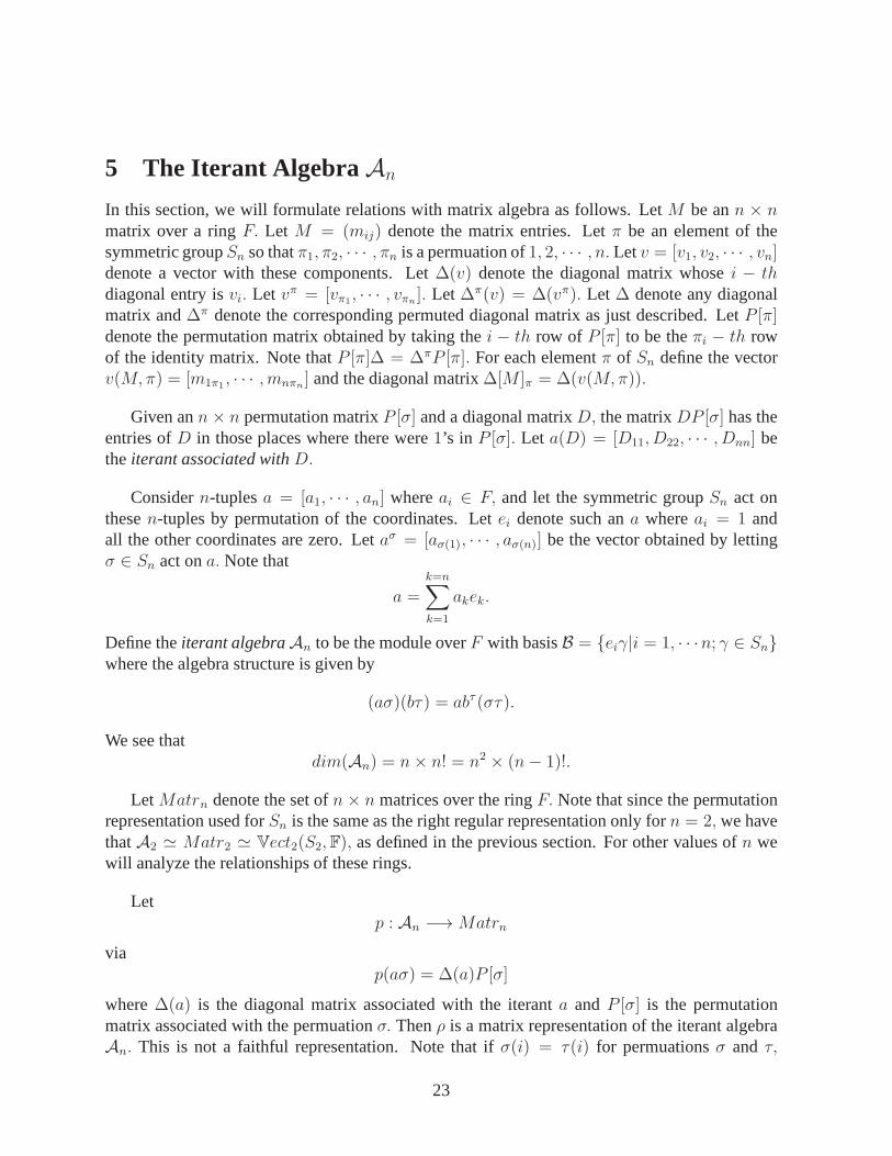
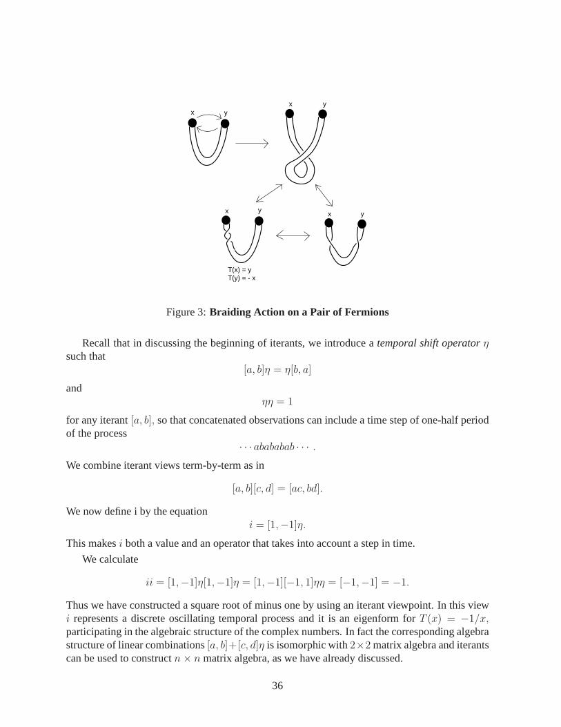
Tk(ck+1) = −ck,andTk is the identity otherwise. This gives a very nice unitary representaton of the Artin braidgroup and it deserves better understanding. See Figure 3 foran illustration of this braiding ofFermions in relation to the topology of a belt that connects them. The relationship with the belt istied up with the fact that in quantum mechanics we must represent rotations of three dimensionalspace as unitary transformations. See [11] for more about this topological view of the physicsof Fermions. In the Figure, we see that the belt does not know which of the two Fermions toannoint with the phase change, but the clever algebra above makes this decision. There is moreto be done in this domain.

It is worth noting that a triple of Majorana fermions saya, b, c gives rise to a representationof the quaternion group. This is a generalization of the well-known association of Pauli matricesand quaternions. We havea2 = b2 = c2 = 1 and they anticommute. LetI = ba, J = cb,K = ac.Then

I2 = J2 = K2 = IJK = −1,giving the quaternions. The operators

A = (1/√2)(1 + I)

B = (1/√2)(1 + J)

C = (1/√2)(1 +K)

braid one another:ABA = BAB,BCB = CBC,ACA = CAC.

This is a special case of the braid group representation described above for an arbitrary list ofMajorana fermions. These braiding operators are entangling and so can be used for universalquantum computation, but they give only partial topological quantum computation due to theinteraction with single qubit operators not generated by them.

35

T(x) = yT(y) = - x

xx

x x

y

y

y

y

Figure 3:Braiding Action on a Pair of Fermions

Recall that in discussing the beginning of iterants, we introduce atemporal shift operatorηsuch that

[a, b]η = η[b, a]

andηη = 1

for any iterant[a, b], so that concatenated observations can include a time step ofone-half periodof the process

· · ·abababab · · · .We combine iterant views term-by-term as in

[a, b][c, d] = [ac, bd].

We now define i by the equationi = [1,−1]η.

This makesi both a value and an operator that takes into account a step in time.

We calculate

ii = [1,−1]η[1,−1]η = [1,−1][−1, 1]ηη = [−1,−1] = −1.

Thus we have constructed a square root of minus one by using aniterant viewpoint. In this viewi represents a discrete oscillating temporal process and it is an eigenform forT (x) = −1/x,participating in the algebraic structure of the complex numbers. In fact the corresponding algebrastructure of linear combinations[a, b]+[c, d]η is isomorphic with2×2 matrix algebra and iterantscan be used to constructn× n matrix algebra, as we have already discussed.

36

Now we can make contact with the algebra of the Majorana fermions. Lete = [1,−1]. Thenwe havee2 = [1, 1] = 1 andeη = [1,−1]η = [−1, 1]η = −eη. Thus we have

e2 = 1,

η2 = 1,

andeη = −ηe.

We can regarde andη as a fundamental pair of Majorana fermions.

Note how the development of the algebra works at this point. We have that

(eη)2 = −1

and so regard this as a natural construction of the square root of minus one in terms of the phasesynchronization of the clock that is the iteration of the reentering mark. Once we have the squareroot of minus one it is natural to introduce another one and call this onei, letting it commute withthe other operators. Then we have the(ieη)2 = +1 and so we have a triple of Majorana fermions:

a = e, b = η, c = ieη

and we can construct the quaternions

I = ba = ηe, J = cb = ie,K = ac = iη.

With the quaternions in place, we have the braiding operators

A =1√2(1 + I), B =

1√2(1 + J), C =

1√2(1 +K),

and can continue as we did above.

9 Laws of Form

This section is a version of a corresponding section in our paper [23]. Here we discuss a for-malism due the G. Spencer-Brown [1] that is often called the “calculus of indications”. Thiscalculus is a study of mathematical foundations with a topological notation based on one symbol,the mark:

.

This single symbol represents a distinction between its owninside and outside. As is evidentfrom Fgure 4, the mark is regarded as a shorthand for a rectangle drawn in the plane and dividingthe plane into the regions inside and outside the rectangle.

37

Figure 4:Inside and Outside

The reason we introduce this notation is that in the calculusof indications the mark caninteract with itself in two possible ways. The resulting formalism becomes a version of Booleanarithmetic, but fundamentally simpler than the usual Boolean arithmetic of0 and1 with its twobinary operations and one unary operation (negation). In the calculus of indications one takesa step in the direction of simplicity, and also a step in the direction of physics. The patterns ofthis mark and its self-interaction match those of aMajorana fermionas discussed in the previoussection. A Majorana fermion is a particle that is its own anti-particle. [7]. We will later see, inthis paper, that by adding braiding to the calculus of indications we arrive at the Fibonacci model,that can in principle support quantum computing.

In the previous section we described Majorana fermions in terms of their algebra of creationand annihilation operators. Here we describe the particle directly in terms of its interactions.This is part of a general scheme called “fusion rules” [8] that can be applied to discrete particleinteracations. A fusion rule represents all of the different particle interactions in the form ofa set of equations. The bare bones of the Majorana fermion consist in a particleP such thatP can interact with itself to produce a neutral particle∗ or produce itselfP. Thus the possibleinteractions are

PP −→ ∗and

PP −→ P.

This is the bare minimum that we shall need. The fusion rule is

P 2 = 1 + P.

This represents the fact thatP can interact with itself to produce the neutral particle (representedas1 in the fusion rule) or itself (represented byP in the fusion rule). .

Is there alinguisticparticle that is its own anti-particle? Certainly we have

∼∼ Q = Q

38

Figure 5:Boxes and Marks

for any propositionQ (in Boolean logic). And so we might write

∼∼−→ ∗

where∗ is a neutral linguistic particle, an identity operator so that

∗Q = Q

for any propositionQ. But in the normal use of negation there is no way that the negation signcombines with itself to produce itself. This appears to ruinthe analogy between negation andthe Majorana fermion. Remarkably, the calculus of indications provides a context in which wecan say exactly that a certain logical particle, the mark, can act as negationandcan interact withitself to produce itself.

In the calculus of indications patterns of non-intersecting marks (i.e. non-intersecting rectan-gles) are calledexpressions.For example in Figure 5 we see how patterns of boxes correspond topatterns of marks.

In Figure 5, we have illustrated both the rectangle and the marked version of the expression.In an expression you can say definitively of any two marks whether one is or is not inside theother. The relationship between two marks is either that oneis inside the other, or that neither isinside the other. These two conditions correspond to the twoelementary expressions shown inFigure 6.

The mathematics in Laws of Form begins with two laws of transformation about these twobasic expressions. Symbolically, these laws are:

1. Calling :=

2. Crossing:= .

39

Figure 6:Translation between Boxes and Marks

The equals sign denotes a replacement step that can be performed on instances of these patterns(two empty marks that are adjacent or one mark surrounding anempty mark). In the first ofthese equations two adjacent marks condense to a single mark, or a single mark expands to formtwo adjacent marks. In the second equation two marks, one inside the other, disappear to formthe unmarked state indicated by nothing at all. That is, two nested marks can be replaced byan empty word in this formal system. Alternatively, the unmarked state can be replaced by twonested marks. These equations give rise to a natural calculus, and the mathematics can begin.For example,any expression can be reduced uniquely to either the marked or the unmarked state.The he following example illustrates the method:

= =

= = .

The general method for reduction is to locate marks that are at the deepest places in the expression(depth is defined by counting the number of inward crossings of boundaries needed to reach thegiven mark). Such a deepest mark must be empty and it is eithersurrounded by another mark, orit is adjacent to an empty mark. In either case a reduction canbe performed by either calling orcrossing.

Laws of Form begins with the following statement. “We take asgiven the idea of a distinctionand the idea of an indication, and that it is not possible to make an indication without drawing adistinction. We take therefore the form of distinction for the form.” Then the author makes thefollowing two statements (laws):

1. The value of a call made again is the value of the call.

2. The value of a crossing made again is not the value of the crossing.

The two symbolic equations above correspond to these statements. First examine the law ofcalling. It says that the value of a repeated name is the valueof the name. In the equation

=

40

one can view either mark as the name of the state indicated by the outside of the other mark. Inthe other equation

= .

the state indicated by the outside of a mark is the state obtained by crossing from the state in-dicated on the inside of the mark. Since the marked state is indicated on the inside, the outsidemust indicate the unmarked state. The Law of Crossing indicates how opposite forms can fit intoone another and vanish into nothing, or how nothing can produce opposite and distinct forms thatfit one another, hand in glove. The same interpretation yields the equation

=

where the left-hand side is seen as an instruction to cross from the unmarked state, and the righthand side is seen as an indicator of the marked state. The markhas a double carry of meaning. Itcan be seen as an operator, transforming the state on its inside to a different state on its outside,and it can be seen as the name of the marked state. That combination of meanings is compatiblein this interpretation.

From the calculus of indications, one moves to algebra. Thus

A

stands for the two possibilities

= ←→ A =

= ←→ A =

In all cases we haveA = A.

By the time we articulate the algebra, the mark can take the role of a unary operator

A −→ A .

But it retains its role as an element in the algebra. Thus begins algebra with respect to this non-numerical arithmetic of forms. The primary algebra that emerges is a subtle precursor to Booleanalgebra. One can translate back and forth between elementary logic and primary algebra:

1. ←→ T

2. ←→ F

3. A ←→∼ A

4. AB ←→ A ∨ B

41

5. A B ←→ A ∧B

6. A B ←→ A⇒ B

The calculus of indications and the primary algebra form an efficient system for working withbasic symbolic logic.

By reformulating basic symbolic logic in terms of the calculus of indications, we have aground in which negation is represented by the markand the mark is also interpreted as a value(a truth value for logic) and these two intepretations are compatible with one another in the for-malism. The key to this compatibility is the choice to represent the value “false” by a literallyunmarked state in the notational plane. With this the empty mark (a mark with nothing on its in-side) can be interpreted as the negation of “false” and hencerepresents “true”. The mark interactswith itself to produce itself (calling) and the mark interacts with itself to produce nothing (cross-ing). We have expanded the conceptual domain of negation so that it satisfies the mathematicalpattern of an abstract Majorana fermion.

Another way to indicate these two interactions symbolically is to use a box,for the markedstate and a blank space for the unmarked state. Then one has two modes of interaction of a boxwith itself:

1. Adjacency:

and

2. Nesting: .

With this convention we take the adjacency interaction to yield a single box, and the nestinginteraction to produce nothing:

=

=

We take the notational opportunity to denote nothing by an asterisk (*). The syntatical rules foroperating the asterisk are Thus the asterisk is a stand-in for no mark at all and it can be erased orplaced wherever it is convenient to do so. Thus

= ∗.

At this point the reader can appreciate what has been done if he returns to the usual form ofsymbolic logic. In that form we that

∼∼ X = X

for all logical objects (propositions or elements of the logical algebra)X. We can summarize thisby writing

∼∼ =

42

as a symbolic statement that is outside the logical formalism. Furthermore, one is committed tothe interpretation of negation as an operator and not as an operand. The calculus of indicationsprovides a formalism where the mark (the analog of negation in that domain) is both a value andan object, and so can act on itself in more than one way.

The Majorana particle is its own anti-particle. It is exactly at this point that physics meets log-ical epistemology. Negation as logical entity is its own anti-particle. Wittgenstein says (Tractatus[27] 4.0621) “ · · · the sign ‘∼’ corresponds to nothing in reality.” And he goes on to say (Tracta-tus5.511) “ How can all-embracing logic which mirrors the world use such special catches andmanipulations? Only because all these are connected into aninfinitely fine network, the greatmirror.” For Wittgenstein in the Tractatus, the negation sign is part of the mirror making it pos-sible for thought to reflect reality through combinations ofsigns. These remarks of Wittgensteinare part of his early picture theory of the relationship of formalism and the world. In our view,the world and the formalism we use to represent the world are not separate. The observer and themark are (formally) identical. A path is opened between logic and physics.

The visual iconics that create via the boxes of half-boxes ofthe calculus of indications amodel for a logical Majorana fermion can also be seen in termsof cobordisms of surfaces. ViewFigure 7. There the boxes have become circles and the interactions of the circles have beendisplayed as evolutions in an extra dimension, tracing out surfaces in three dimensions. Thecondensation of two circles to one is a simple cobordism betweem two circles and a single circle.The cancellation of two circles that are concentric can be seen as the right-hand lower cobordismin this figure with a level having a continuum of critical points where the two circles cancel. Asimpler cobordism is illustrated above on the right where the two circles are not concentric, butnevertheless are cobordant to the empty circle. Another wayof putting this is that two topologicalclosed strings can interact by cobordism to produce a singlestring or to cancel one another. Thusa simple circle can be a topological model for a Majorana fermion.

In [23, 24] we detail how the Fibonacci model for anyonic quantum computing can be con-structed by using a version of the two-stranded bracket polynomial and a generalization of Pen-rose spin networks. This is a fragment of the Temperly-Lieb recoupling theory [12].

9.1 The Square Root of Minus One Revisited

So far we have seen that the mark can represent the fusion rules for a Majorana fermion sinceit can interact with itself to produce either itself or nothing. But we have not yet seen the anti-commuting fermion algebra emerge from this context of making a distinction. Remarkably, thisalgebra does emerge when one looks at the mark recursively.

Consider the transformationF (X) = X .

43

Figure 7:Calling, Crossing and Cobordism

If we iterate it and take the limit we find

G = F (F (F (F (· · · )))) = ...

an infinite nest of marks satisfying the equation

G = G .

With G = F (G), I say thatG is aneigenformfor the transformationF. See Figure 8 for anillustration of this nesting with boxes and an arrow that points inside the reentering mark toindicate its appearance inside itself. If one thinks of the mark itself as a Boolean logical value,then extending the language to include the reentering markG goes beyond the boolean. We willnot detail here how this extension can be related to non-standard logics, but refer the reader to[12]. Taken at face value the reentering mark cannot be just marked or just unmarked, for by itsvery definition, if it is marked then it is unmarked and if it isunmarked then it is marked. Inthis sense the reentering mark has the form of a self-contradicting paradox. There is no paradoxsince we do not have to permanently assign it to either value.The simplest interpretation of thereentering mark is that it is temporal and that it representsan oscillation between markednessand unmarkedness. In numerical terms it is a discrete dynamical system oscillating between+1(marked) and−1 (not marked).

With the reentering mark in mind consider now the transformation on real numbers given by

T (x) = −1/x.

This has the fixed pointsi and−i, the complex numbers whose squares are negative unity. Butlets take a point of view more directly associated with the analogy of the recursive mark. Begin

44

... =

Figure 8:

by starting with a simple periodic process that is associated directly with the classical attempt tosolve fori as a solution to a quadratic equation. We take the point of view that solvingx2 = ax+bis the same (whenx 6= 0) as solving

x = a + b/x,

and hence is a matter of finding a fixed point. In the case ofi we have

x2 = −1and so desire a fixed point

x = −1/x.There are no real numbers that are fixed points for this operator and so we consider the oscillatoryprocess generated by

T (x) = −1/x.The fixed point would satisfy

i = −1/iand multiplying, we get that

ii = −1.On the other hand the iteration ofT yields

1, T (1) = −1, T (T (1)) = +1, T (T (T (1))) = −1,+1,−1,+1,−1, · · · .The square root of minus one is a perfect example of an eigenform that occurs in a new andwider domain than the original context in which its recursive process arose. The process has nofixed point in the original domain. At this point we enter onceagain the domain of iterants andparticularly the discussion of Section 6 where we see the square root of minus one as a clock.

There is one more comment that is appropriate for this section. Recall that a pair of Majoranafermions can be assembled to form a single standard fermion.In our case we have the spatialand temporal iterant componentse = [1,−1] andη with eη = −ηe. We can regarde andη as afundamental pair of Majorana fermions. This is a formal correspondence, but it is striking howthis Marjorana fermion algebra emerges from an analysis of the recursive nature of the reenteringmark, while the fusion algebra for the Majorana fermion emerges from the distinctive propertiesof the mark itself. We see how the seeds of the fermion algebralive in this extended logicalcontext.

45

The corresponding standard fermion annihilation and creation operators are then given by theformulas below.

ψ = (e + iη)/2

andψ† = (e− iη)/2.

Sincee represents a spatial view of the basic discrete oscillationandη is the time-shift operatorfor this oscillation it is of interest to note that the standard fermion built by these two can beregarded as a quantum of spacetime, retrieved from the way that we decomposed the processinto space and time. Since all this is initially built in relation to extending the Boolean logicof the mark to a non-boolean recursive context, there is further analysis needed of the relationof the physics and the logic. We have only begun the analysis here. The crux of the matter isthat two dimensional physics depends upon a plane space in which a simple closed curve makesa distinction between inside and outside in order for the braiding and phases to be significant.This same property of distinction in the plane is what gives aplane space the linguistic power torepresent language and logic. This correspondence in not anaccident and deserves further study!

10 The Dirac Equation and Majorana Fermions

We now construct the Dirac equation. This may sound circular, in that the fermions arise fromsolving the Dirac equation, but in fact the algebra underlying this equation has the same propertiesas the creation and annihilation algebra for fermions, so itis by way of this algebra that we willcome to the Dirac equation. If the speed of light is equal to1 (by convention), then energyE,momentump and massm are related by the (Einstein) equation

E2 = p2 +m2.

Dirac constructed his equation by looking for an algebraic square root ofp2+m2 so that he couldhave a linear operator forE that would take the same role as the Hamiltonian in the Schroedingerequation. We will get to this operator by first taking the casewherep is a scalar (we use onedimension of space and one dimension of time.). LetE = αp+ βm whereα andβ are elementsof a a possibly non-commutative, associative algebra. Then

E2 = α2p2 + β2m2 + pm(αβ + βα).

Hence we will satisfiyE2 = p2 + m2 if α2 = β2 = 1 andαβ + βα = 0. This is our familiarClifford algebra pattern and we can use the iterant algebra generated bye andη if we wish. Then,because the quantum operator for momentum is−i∂/∂x and the operator for energy isi∂/∂t, wehave the Dirac equation

i∂ψ/∂t = −iα∂ψ/∂x + βmψ.

LetO = i∂/∂t + iα∂/∂x − βm

46

so that the Dirac equation takes the form

Oψ(x, t) = 0.

Now note that

Oei(px−Et) = (E − αp− βm)ei(px−Et).

We let

∆ = (E − αp− βm)

and let

U = ∆βα = (E − αp− βm)βα = βαE + βp− αm,

then

U2 = −E2 + p2 +m2 = 0.

This nilpotent element leads to a (plane wave) solution to the Dirac equation as follows: We haveshown that

Oψ = ∆ψ

for ψ = ei(px−Et). It then follows that

O(βα∆βαψ) = ∆βα∆βαψ = U2ψ = 0,

from which it follows that

ψ = βαUei(px−Et)

is a (plane wave) solution to the Dirac equation.

In fact, this calculation suggests that we should multiply the operatorO by βα on the right,obtaining the operator

D = Oβα = iβα∂/∂t + iβ∂/∂x − αm,

and the equivalent Dirac equation

Dψ = 0.

In fact for the specificψ above we will now haveD(Uei(px−Et)) = U2ei(px−Et) = 0. This ideaof reconfiguring the Dirac equation in relation to nilpotentalgebra elementsU is due to PeterRowlands [26]. Rowlands does this in the context of quaternion algebra. Note that the solutionto the Dirac equation that we have found is expressed in Clifford algebra or iterant algebra form.It can be articulated into specific vector solutions by usingan iterant or matrix representation ofthe algebra.

47

We see thatU = βαE + βp − αm with U2 = 0 is really the essence of this plane wavesolution to the Dirac equation. This means that a natural non-commutative algebra arises directlyand can be regarded as the essential information in a Fermion. It is natural to compare this algebrastructure with algebra of creation and annihilation operators that occur in quantum field theory.to this end, let

U † = αβE + αp− βm.Here we regardU † as a formal counterpart to complex conjugation, since in thesplit quaternionalgebra we have not yet constructed commuting square roots of negative one. We then find thatwith

A = U + U † = (α+ β)(p−m)

andB = U − U † = 2βαE + (β − α)(p−m)

that

[A√

2(p−m)]2 = 1

and

[iB√

2(p +m)]2 = 1,

with i a commuting square root of negative one, giving the underlying Majorana Fermion opera-tors for our Dirac Fermion. The operatorsU andU † satisfy the usual commutation relations forthe annihilation and creation operators for a Fermion.

It is worth noting how the Pythgorean relationshipE2 = p2 + m2 interacts here with theClifford algebra ofα andβ. We have

U † = pα +mβ + αβE

U = pβ +mα + βαE

with(U †)2 = U2 = 0,

U + U † = (p+m)(α + β),

U − U † = (p−m)(α− β) + 2Eαβ.

This implies that(U + U †)2 = 2(p+m)2

(U − U †)2 = 2(p−m)2 − 4E2 = 2[p2 +m2 − 2pm− 2p2 − 2m2] = −2(p+m)2.

From this we easily deduce that

UU † + U †U = 2(p+m)2,

and this can be normalized to equal1.

48

10.1 Another version ofU andU †

We start withψ = ei(px−Et) and the operators

E = i∂/∂t

andp = −i∂/∂x

so thatEψ = Eψ

andpψ = pψ.

The Dirac operator isO = E − αp− βm

and the modified Dirac operator is

D = Oβα = βαE + βp− αm,

so thatDψ = (βαE + βp− αm)ψ = Uψ.

If we letψ = ei(px+Et)

(reversing time), then we have

Dψ = (−βαE + βp− αm)ψ = U †ψ,

giving a definition ofU † corresponding to the anti-particle forUψ.

We haveU = βαE + βp− αm

andU † = −βαE + βp− αm

Note that here we have

(U + U †)2 = (2βp+ αm)2 = 4(p2 +m2) = 4E2,

and(U − U †)2 = −(2βαE)2 = −4E2.

We have thatU2 = (U †)2 = 0

49

andUU † + U †U = 4E2.

Thus we have a direct appearance of the Fermion algebra corresponding to the Fermion planewave solutions to the Dirac equation. Furthermore, the decomposition ofUandU † into the cor-responding Majorana Fermion operators corresponds toE2 = p2 +m2. Normalizing by dividingby 2E we have

A = (βp+ αm)/E

andB = iβα.

so thatA2 = B2 = 1

andAB +BA = 0.

thenU = (A+Bi)E

andU † = (A−Bi)E,

showing how the Fermion operators are expressed in terms of the simpler Clifford algebra ofMajorana operators (split quaternions once again).

10.2 Writing in the Full Dirac Algebra

We have written the Dirac equation so far in one dimension of space and one dimension oftime. We give here a way to boost the formalism directly to three dimensions of space. Wetake an independent Clifford algebra generated byσ1, σ2, σ3 with σ2

i = 1 for i = 1, 2, 3 andσiσj = −σjσi for i 6= j. Now assume thatα and β as we have used them above generatean independent Clifford algebra that commutes with the algebra of theσi. Replace the scalarmomentump by a3-vector momentump = (p1, p2, p3) and letp • σ = p1σ1 + p2σ2 + p3σ3. Wereplace∂/∂x with ∇ = (∂/∂x1, ∂/∂x2, ∂/∂x2) and∂p/∂x with∇ • p.

We then have the following form of the Dirac equation.

i∂ψ/∂t = −iα∇ • σψ + βmψ.

LetO = i∂/∂t + iα∇ • σ − βm

so that the Dirac equation takes the form

Oψ(x, t) = 0.

50

In analogy to our previous discussion we let

ψ(x, t) = ei(p•x−Et)

and construct solutions by first applying the Dirac operatorto thisψ. The two Clifford algebrasinteract to generalize directly the nilpotent solutions and Fermion algebra that we have detailedfor one spatial dimension to this three dimensional case. Tothis purpose the modified Diracoperator is

D = iβα∂/∂t + β∇ • σ − αm.And we have that

Dψ = Uψ

whereU = βαE + βp • σ − αm.

We have thatU2 = 0 andUψ is a solution to the modified Dirac Equation, just as before. And justas before, we can articulate the structure of the Fermion operators and locate the correspondingMajorana Fermion operators. We leave these details to the reader.

10.3 Majorana Fermions at Last

There is more to do. We will end with a brief discussion makingDirac algebra distinct from theone generated byα, β, σ1, σ2, σ3 to obtain an equation that can have real solutions. This was thestrategy that Majorana [7] followed to construct his Majorana Fermions. A real equation can havesolutions that are invariant under complex conjugation andso can correspond to particles that aretheir own anti-particles. We will describe this Majorana algebra in terms of the split quaternionsǫ andη. For convenience we use the matrix representation given below. The reader of this papercan substitute the corresponding iterants.

ǫ =

(

−1 00 1

)

, η =

(

0 11 0

)

.

Let ǫ andη generate another, independent algebra of split quaternions, commuting with the firstalgebra generated byǫ and η. Then a totally real Majorana Dirac equation can be written asfollows:

(∂/∂t + ηη∂/∂x+ ǫ∂/∂y + ǫη∂/∂z − ǫηηm)ψ = 0.

To see that this is a correct Dirac equation, note that

E = αxpx + αypy + αzpz + βm

(Here the “hats” denote the quantum differential operatorscorresponding to the energy and mo-mentum.) will satisfy

E2 = px2 + py

2 + pz2 +m2

51

if the algebra generated byαx, αy, αz, β has each generator of square one and each distinct pairof generators anti-commuting. From there we obtain the general Dirac equation by replacingEby i∂/∂t, andpx with −i∂/∂x (and same fory, z).

(i∂/∂t + iαx∂/∂x + iαy∂/∂y + iαz∂/∂y − βm)ψ = 0.

This is equivalent to

(∂/∂t + αx∂/∂x + αy∂/∂y + αz∂/∂y + iβm)ψ = 0.

Thus, here we takeαx = ηη, αy = ǫ, αz = ǫη, β = iǫηη,

and observe that these elements satisfy the requirements for the Dirac algebra. Note how we havea significant interaction between the commuting square rootof minus one (i) and the elementǫηof square minus one in the split quaternions. This brings us back to our original considerationsabout the source of the square root of minus one. Both viewpoints combine in the elementβ = iǫηη that makes this Majorana algebra work. Since the algebra appearing in the MajoranaDirac operator is constructed entirely from two commuting copies of the split quaternions, thereis no appearance of the complex numbers, and when written outin 2 × 2 matrices we obtaincoupled real differential equations to be solved. Clearly this ending is actually a beginning of anew study of Majorana Fermions. That will begin in a sequel tothe present paper.

References

[1] G. Spencer–Brown, “Laws of Form,” George Allen and UnwinLtd. London (1969).

[2] Kauffman, L. [1985], Sign and Space, In Religious Experience and Scientific Paradigms.Proceedings of the 1982 IASWR Conference, Stony Brook, New York: Institute of Ad-vanced Study of World Religions, (1985), 118-164.

[3] Kauffman, L. [1987], Self-reference and recursive forms, Journal of Social and BiologicalStructures (1987), 53-72.

[4] Kauffman, L. [1987], Special relativity and a calculus of distinctions. Proceedings of the9th Annual Intl. Meeting of ANPA, Cambridge, England (1987). Pub. by ANPA West, pp.290-311.

[5] Kauffman, L. [1987], Imaginary values in mathematical logic. Proceedings of the Seven-teenth International Conference on Multiple Valued Logic,May 26-28 (1987), Boston MA,IEEE Computer Society Press, 282-289.

[6] Kauffman, L. H., Knot Logic, InKnots and Applicationsed. by L. Kauffman, World Scien-tific Pub. Co., (1994), pp. 1-110.

52

[7] E. Majorana, A symmetric theory of electrons and positrons, I Nuovo Cimento,14 (1937),pp. 171-184.

[8] G. Moore and N. Read, Noabelions in the fractional quantum Hall effect,Nuclear PhysicsB360(1991), 362 - 396.

[9] V. Mourik,K. Zuo, S. M. Frolov, S. R. Plissard, E.P.A.M. Bakkers, L.P. Kouwenhuven,Signatures of Majorana fermions in hybred superconductor-semiconductor devices, arXiv:1204.2792.

[10] Kauffman, Louis H. [2002], Biologic.AMS Contemporary Mathematics Series, Vol. 304,(2002), pp. 313 - 340.

[11] Kauffman,Louis H.[1991,1994,2001,2012],Knots and Physics,World Scientific Pub.

[12] L.H. Kauffman, Temperley-Lieb Recoupling Theory and Invariants of Three-Manifolds,Princeton University Press, Annals Studies114(1994).

[13] Kauffman, Louis H. [2002], Time imaginary value, paradox sign and space, inComputingAnticipatory Systems, CASYS - Fifth International Conference, Liege, Belgium (2001) ed.by Daniel Dubois, AIP Conference Proceedings Volume 627 (2002).

[14] Kauffman,Louis H. and Noyes,H. Pierre [1996], Discrete Physics and the Derivation ofElectromagnetism from the formalism of Quantum Mechanics,Proc. of the Royal Soc.Lond. A, 452, pp. 81-95.

[15] Kauffman,Louis H. and Noyes,H. Pierre [1996], Discrete Physics and the Dirac Equation,Physics Letters A, 218 ,pp. 139-146.

[16] Kauffman, Louis H. [1998], Noncommutativity and discrete physics,Physica D 120(1998), 125-138.

[17] Kauffman, Louis H. [1998], Space and time in discrete physics,Intl. J. Gen. Syst.Vol. 27,Nos. 1-3, 241-273.

[18] Kauffman, Louis H. [1999], A non-commutative approachto discrete physics, inAspects II- Proceedings of ANPA 20, 215-238.

[19] Kauffman, Louis H. [2003], Non-commutative calculus and discrete physics, inBoundaries- Scientific Aspects of ANPA 24, 73-128.

[20] Kauffman, Louis H. [2004], Non-commutative worlds,New Journal of Physics 6, 2-46.

[21] Kauffman, Louis H., Non-commutative worlds and classical constraints. in “Scientific Es-says in Honor of Pierre Noyes on the Occasion of His 90-th Birthday”, edited by JohnAmson and Louis H. Kaufman, World Scientific Pub. Co. (2013),pp. 169-210.

53

[22] Louis H. Kauffman, Differential geometry in non-commutative worlds, in “Quantum Grav-ity - Mathematical Models and Experimental Bounds”, editedby B. Fauser, J. Tolksdorfand E. Zeidler, Birkhauser (2007), pp. 61 - 75.

[23] Kauffman, Louis H. [2012], Knot Logic and Topological Quantum Computing with Majo-rana Fermions, (to appear).

[24] Kauffman, Louis H.; Lomonaco, Samuel J., Jr.q-deformed spin networks, knot polynomialsand anyonic topological quantum computation. J. Knot Theory Ramifications 16 (2007), no.3, 267–332.

[25] D. E. Littlewood, “The Skeleton Key of Mathematics”, Harper Torchbook Edition (1960).

[26] Peter Rowlands, “Zero to Infinity - The Foundations of Physics”, Series on Knots and Ev-erything - Volume 41, World Scientific Publishing Co., 2007.

[27] L. Wittgenstein, “Tractatus Logico - Philosophicus”,New York: Harcourt, Brace and Com-pany, Inc., London: Kegan Paul, Trench, Trubner and Co. Ltd.(1922).

54