it is easy to determine whether a given integer is prime

BULLETIN (New Series) OF THEAMERICAN MATHEMATICAL SOCIETYVolume 42, Number 1, Pages 3–38S 0273-0979(04)01037-7Article electronically published on September 30, 2004

IT IS EASY TO DETERMINE WHETHER A GIVEN INTEGERIS PRIME

ANDREW GRANVILLE

Dedicated to the memory of W. ‘Red’ Alford, friend and colleague

Abstract. “The problem of distinguishing prime numbers from compositenumbers, and of resolving the latter into their prime factors is known to beone of the most important and useful in arithmetic. It has engaged the industryand wisdom of ancient and modern geometers to such an extent that it wouldbe superfluous to discuss the problem at length. Nevertheless we must confessthat all methods that have been proposed thus far are either restricted to veryspecial cases or are so laborious and difficult that even for numbers that donot exceed the limits of tables constructed by estimable men, they try thepatience of even the practiced calculator. And these methods do not apply atall to larger numbers ... It frequently happens that the trained calculator willbe sufficiently rewarded by reducing large numbers to their factors so that itwill compensate for the time spent. Further, the dignity of the science itselfseems to require that every possible means be explored for the solution of aproblem so elegant and so celebrated ... It is in the nature of the problemthat any method will become more complicated as the numbers get larger.Nevertheless, in the following methods the difficulties increase rather slowly... The techniques that were previously known would require intolerable laboreven for the most indefatigable calculator.”

—from article 329 of Disquisitiones Arithmeticae (1801) by C. F. Gauss

There are few better known or more easily understood problems in pure mathe-matics than the question of rapidly determining whether a given integer is prime.As we read above, the young Gauss in his first book Disquisitiones Arithmeticaeregarded this as a problem that needs to be explored for “the dignity” of our sub-ject. However it was not until the modern era, when questions about primalitytesting and factoring became a central part of applied mathematics,1 that therewas a large group of researchers endeavoring to solve these questions. As we shallsee, most of the key ideas in recent work can be traced back to Gauss, Fermat andother mathematicians from times long gone by, and yet there is also a modern spin:With the growth of computer science and a need to understand the true difficultyof a computation, Gauss’s vague assessment “intolerable labor” was only recently

Received by the editors January 27, 2004, and, in revised form, August 19, 2004.2000 Mathematics Subject Classification. Primary 11A51, 11Y11; Secondary 11A07, 11A41,

11B50, 11N25, 11T06.L’auteur est partiellement soutenu par une bourse du Conseil de recherches en sciences na-

turelles et en genie du Canada.1Because of their use in the data encryption employed by public key cryptographic schemes;

see section 3a.

c©2004 American Mathematical SocietyReverts to public domain 28 years from publication

3

4 ANDREW GRANVILLE

clarified by “running time estimates”, and of course our desktop computers aretoday’s “indefatigable calculators”.

Fast factoring remains a difficult problem. Although we can now factor an arbi-trary large integer far faster than in Gauss’s day, still a 400 digit integer which isthe product of two 200 digit primes is typically beyond practical reach.2 This is justas well since the safety of electronic business transactions, such as when you useyour ATM card or purchase something with your credit card over the Web dependson the intractability of such problems!

On the other hand we have been able to rapidly determine whether quite largenumbers are prime for some time now. For instance recent algorithms can test anarbitrary integer with several thousand digits for primality within a month on aPentium IV,3 which allows us to easily create the cryptographic schemes referred toabove. However the modern interpretation of Gauss’s dream was not realized untilAugust 2002, when three Indian computer scientists—Manindra Agrawal, NeerajKayal and Nitin Saxena—constructed a “polynomial time deterministic primalitytest”, a much sought-after but elusive goal of researchers in the algorithmic numbertheory world. Most shocking was the simplicity and originality of their test ...whereas the “experts” had made complicated modifications on existing tests togain improvements (often involving great ingenuity), these authors rethought thedirection in which to push the usual ideas with stunning success.4 Their algorithmis based on the following elegant characterization of prime numbers.

Agrawal, Kayal and Saxena. For given integer n ≥ 2, let r be a positive integer< n, for which n has order > (log n)2 modulo r. Then n is prime if and only if

• n is not a perfect power,• n does not have any prime factor ≤ r,• (x + a)n ≡ xn + a mod (n, xr − 1) for each integer a, 1 ≤ a ≤

√r log n.

We will discuss the meaning of technical notions like “order” and “≡” a littlelater. For the reader who has encountered the terminology before, one word ofwarning: The given congruences here are between polynomials in x, and not betweenthe two sides evaluated at each integer x.

At first sight this might seem to be a rather complicated characterization of theprime numbers. However we shall see that this fits naturally into the historicalprogression of ideas in this subject, is not so complicated (compared to some otherideas in use), and has the great advantage that it is straightforward to develop intoa fast algorithm for proving the primality of large primes.

Perhaps now is the moment to clarify our goals:

2My definition will stretch the usual use of the word “practical” by erring on the cautiousside: I mean a calculation that can be done using all computers that have or will be built for thenext century, assuming that improvements in technology do not happen much faster than we haveseen in the last couple of decades (during which time computer technology has, by any standards,developed spectacularly rapidly).

3This is not to be confused with algorithms that test the primality of integers of a specialshape. For example, the GIMPS project (the Great Internet Mersenne Prime Search) routinelytests Mersenne numbers, numbers of the form 2p − 1, for primality which have millions of digits.However these algorithms have very limited applicability.

4Though some experts had actually developed many of the same ideas; see section 6.5 forexample.

IT IS EASY TO DETERMINE WHETHER A GIVEN INTEGER IS PRIME 5

1.1. Our objective is to find a “quick” foolproof algorithm to determine whethera given integer is prime. Everyone knows trial division, in which we try to dividen by every integer m in the range 2 ≤ m ≤ √

n. The number of steps in thisalgorithm will be at least the number of integers m we consider, which is somethinglike

√n in the worst case (when n is prime). Note that

√n is roughly 2d/2 where d

is the number of digits of n when written in binary (and d is roughly log n where,here and throughout, we will take logarithms in base 2).

The objective in this area has been to come up with an algorithm which worksin no more than cdA steps in the worst case, where c and A are some fixed pos-itive constants, that is, an algorithm which works in Polynomial Time (which isoften abbreviated as P). With such an algorithm one expects that one can rapidlydetermine whether any “reasonably sized” integer is prime. This is the moderninterpretation of Gauss’s dream.

Before the work of Agrawal, Kayal and Saxena the fastest that we could proveany primality testing algorithm worked was something like dc log log d steps,5 forsome constant c > 0. At first sight this might seem far away from a polynomialtime algorithm, since log log d goes to infinity as d → ∞. However log log d goes toinfinity “with great dignity” (as Dan Shanks put it), and in fact never gets largerthan 7 in practice!6 By January 2004 such algorithms were able7 to prove theprimality of 10,000 digit primes (in base 10), an extraordinary achievement.

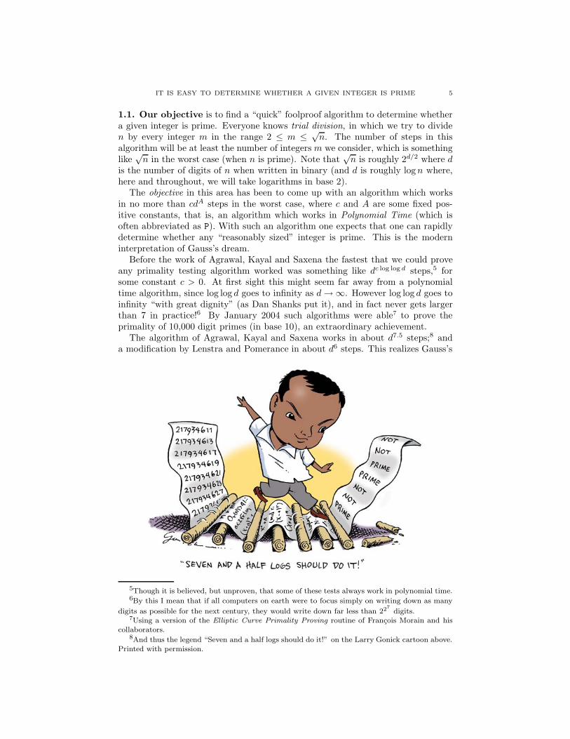
The algorithm of Agrawal, Kayal and Saxena works in about d7.5 steps;8 anda modification by Lenstra and Pomerance in about d6 steps. This realizes Gauss’s

5Though it is believed, but unproven, that some of these tests always work in polynomial time.6By this I mean that if all computers on earth were to focus simply on writing down as many

digits as possible for the next century, they would write down far less than 227digits.

7Using a version of the Elliptic Curve Primality Proving routine of Francois Morain and hiscollaborators.

8And thus the legend “Seven and a half logs should do it!” on the Larry Gonick cartoon above.Printed with permission.

6 ANDREW GRANVILLE

dream, or, in modern language, implies that “Primes are in P”. No one has yetwritten a computer program implementing these algorithms which comes close toproving primality of primes as large as those 10,000 digit primes discussed above.

Building on a clever idea of Berrizbeitia, Bernstein (and, independently, Mi-hailescu and Avanzi) gave a modification that will “almost certainly” run in aroundd4 bit operations. There is hope that this can be used to write a computer programwhich will prove the primality of 10,000 digit primes rapidly. This is a challengefor the near future.

1.2. This article is an elaboration of a lecture given at the “Current Events” spe-cial session during the 2004 annual meeting of the American Mathematical Society.The purpose is to explain the AKS9 primality test, with complete proofs, and toput the result and ideas in appropriate historical context.

To start with I would like to discuss simpler ideas from the subject of primal-ity testing, focusing on some that are closely related to the AKS algorithm. Inthe process we will discuss the notions of complexity classes from theoretical com-puter science10 and in particular introduce the “P �=NP” problem, one of the greatchallenges of mathematics for the new millennium.

We will see that most of the key ideas used to prove the theorem above werealready in broad circulation, and so it is surprising that such an approach was notsuccessfully completed earlier. I believe that there were two reasons for this —first, the way in which these classical ideas were combined was clever and originalin several aspects. Second the authors are not number theorists and came at itfrom a little bit of a different angle; in particular not being so aware of what wassupposedly too difficult, they trod where number theorists fear to tread.

In the third section we will discuss “running time” of algorithms in some detailand how they are determined, and so analyze the AKS algorithm.

In the fourth, and perhaps most interesting, section, we give the proof of themain results. In fact Agrawal et al. have produced two manuscripts, the secondgiving an even easier proof than the first, and we shall discuss both these proofsand relevant background information.

To prove the best running times for the algorithm it is necessary to employ toolsof analytic number theory. In section 5 we introduce the reader to some beautifultheorems about the distribution of primes that should be better known and usethem to prove the claimed running times.

In section 6, we discuss the modified AKS algorithm of Berrizbeitia and Bern-stein, as well as Lenstra’s finite field primality test,11 and then, in section 7, theAKS-inspired algorithm of Lenstra and Pomerance.

Since the first announcement of this result in August 2002 there have been morethan a dozen preprints circulating containing interesting ideas concerning the AKSalgorithm, though none have yet appeared in print. I have thus succumbed to thetemptation to include several of these ideas in the final section, in part becausethey are quite accessible, and in part because they are too elegant to leave out.

9An abbreviation for Agrawal, Kayal and Saxena.10The cost of conveying the essence, rather than the details, of these notions is that our

definitions will be a little awry, but not in a way that effects the key considerations in our context.11Since this twenty-year-old test has much in common with the AKS test and has a running

time that is not far from polynomial.


Bernstein reckons that these and other ideas for improving the AKS algorithmresult in a speed up by a factor of about two million, although, he cautions, “twomillion times faster is not necessarily fast.”

1.3. Undergraduate research experiences. Manindra Agrawal is a facultymember in the Computer Science Department at the Indian Institute of Technol-ogy in Kanpur, India. The fundamental approach taken here to primality testingwas developed by Agrawal in conjunction with two bachelor’s theses which we willdiscuss in section 8.5, the first completed by Pashant Pandey and Rajat Bhat-tacharjee in 2001, the second completed by Neeraj Kayal and Nitin Saxena in 2002.Later that summer they developed what they had done into a first version of thecharacterization of primes given above. There can have been few undergraduateresearch experiences with such a successful outcome!

2. Primality testing and the Child’s Binomial Theorem

2.1. Recognizing primes. To find a primality test that works faster than trialdivision we look for other simple characterizations of prime numbers which mightbe used in a more efficient algorithm. If you have studied a little number theory,then a simple characterization of the primes that comes to mind is:

Wilson’s Theorem (1770). Integer n ≥ 2 is prime if and only if n divides(n − 1)! + 1.

In trying to convert this elegant characterization into a fast algorithm we run intothe problem that there is no obvious way to compute (n − 1)! rapidly (or even(n − 1)! (mod n)).

Another idea is to use Matijasevic’s unbelievable polynomial (1970) which wasessential in resolving Hilbert’s Tenth Problem. He showed how to construct apolynomial with integer coefficients (in several variables) such that whenever onesubstitutes in integers for the variables and gets a positive value, then that value is aprime number; moreover, every prime number will be such a value of the polynomial.(In fact one can construct such a polynomial of degree 10 in 26 variables.) Howeverit is far from evident how to quickly determine whether a given integer is a valuetaken by this polynomial (at least no one to date has found a nice way to do so),and so this seems to be a hopeless approach.

Primes come up in many different places in the mathematical literature, andsome of these suggest ways to distinguish primes from composites. Those of us whoare interested in primality testing always look at anything new with one eye opento this application, and yet finding a fast primality testing algorithm has remainedremarkably elusive. The advent of the AKS algorithm makes me wonder whetherwe have missed some such algorithm, something that one could perform in a fewminutes, by hand, on any enormous number.

Such speculation brings me to a passage from Oliver Sacks’ The man who mistookhis wife for a hat, in which he tells us of a pair of severely autistic twins with aphenomenal memory for numbers and a surprising aesthetic. Sacks discovered thetwins holding a purely numerical conversation, in which one would mention a six-digit number, the other would listen, think for a moment and then beam a smile ofcontented pleasure before responding with another six-digit number for his brother.After listening for a while, Sacks wrote the numbers down and, following a hunch,determined that all of the numbers exchanged were primes. The next day, armed

8 ANDREW GRANVILLE

with a table of primes, Sacks butted into their conversation, venturing an eight-digit prime and eliciting, after a short pause, enthusiastic smiles from the twins.Now the twins kept on going, increasing the number of digits at each turn, untilthey were trading (as far as Sacks could tell) twenty-digit prime numbers. So howdid the twins do it? Perhaps we will never know, since the twins were eventuallyseparated, became “socialized” and forgot their amazing algorithm!

Since we do not know of any such shortcuts, I wish to move on to a propertyof prime numbers that has fascinated mathematicians since antiquity and has beendeveloped into several key approaches to primality testing.

2.2. The Child’s Binomial Theorem. The binomial theorem gives a formulafor expanding (x + y)n as a sum of multiples of terms xiyn−i, namely

(2.1) (x + y)n =n∑

i=0

(n

i

)xiyn−i

where(ni

)= n!

i!(n−i)! and m! = m(m − 1)(m − 2) . . . 3.2.1. This is one of the firstsignificant formulas that students learn in high school, though, perhaps due toits complicated structure, all too often we find university undergraduates who areunable to recall this formula and indeed who write down the (generally) incorrect

(2.2) (x + y)n = xn + yn.

This is called, by some, the Child’s Binomial Theorem. Despite (2.2) being wrongin general, we shall be interested in those (unlikely) circumstances in which thisformula is actually correct!

One of the most amazing properties of prime numbers, discovered12 by Fermataround 1637, is that if n is prime, then n divides an−a for all integers a. This maybe rewritten13 as

(2.3) an ≡ a mod n

for all integers a and primes n; and thus

(2.4) (x + y)n ≡ x + y ≡ xn + yn (mod n)

for all integers x, y and primes n.The integers form equivalence classes mod n, and this set of equivalence classes

forms the ring denoted Z/n (or Z/nZ). If n is prime, then Z/n is a field, and sothe last equation may be rewritten as (2.2) in Z/n.

Actually (2.4) holds also for variables x and y when n is prime, as we shall seelater in section 2.8, a true Child’s Binomial Theorem. It is easy to deduce Fermat’sLittle Theorem from the Child’s Binomial Theorem by induction: Evidently (2.3)holds for a = 1, and if (2.3) holds for all a < A, then taking x = A − 1, y = 1in (2.4) gives An ≡ (A − 1)n + 1n ≡ (A − 1) + 1 = A (mod n) by the inductionhypothesis.

2.3. Composite numbers may sometimes be recognized when they do nothave a particular property that primes have. For example, as we noted above

12There is evidence that this was known for a = 2 far earlier.13For the uninitiated, we say that a ≡ b (mod m) if and only if m divides b − a; the main

advantage of this notation is that we can do most regular arithmetic operations (mod m).


Fermat’s Little Theorem (1637). If n is prime, then n divides an − a for allintegers a.

Therefore conversely, if integer n does not divide an − a for some integer a, then nis composite. For example, taking a = 2 we calculate that

21001 ≡ 123 (mod 1001),

so we know that 1001 is composite.We might ask whether this always works. In other words,

Is it true that if n is composite, then n does not divide 2n − 2?For, if so, we have a very nice way to distinguish primes from composites. Unfor-tunately the answer is “no” since, for example,

2341 ≡ 2 (mod 341),

but 341 = 11 × 31. Note though that by taking a = 3 above we get

3341 ≡ 168 (mod 341),

so we can still use these ideas to prove that 341 is composite.But then we might ask whether this always works, whether there is always some

value of a that helps us prove a composite n is indeed composite.In other words,

Is it true that if n is composite, then thereis some integer a for which n does not divide an − a?

Again the answer is “no” since 561 divides a561 − a for all integers a, yet 561 =3 × 11 × 17. Composite integers n which divide an − a for all integers a arecalled Carmichael numbers, 561, 1105 and 1729 being the smallest three exam-ples. Carmichael numbers are a nuisance, masquerading as primes like this, thoughcomputationally they only appear rarely. Unfortunately it was recently proved thatthere are infinitely many of them and that when we go out far enough they are notso rare as it first appears.

2.4. Square roots of 1. In a field, a non-zero polynomial of degree d has at mostd roots. For the particular example x2 − 1 this implies that 1 has just two squareroots mod p, a prime > 2, namely 1 and −1.

What about mod composite n? For the smallest odd composite n with morethan one prime factor, that is n = 15, we find 12 ≡ 42 ≡ 112 ≡ 142 (mod 15); thatis, there are four square roots of 1 (mod 15). And this is true in general: There areat least four distinct square roots of 1 (mod n) for any odd n which is divisible bytwo distinct primes. Thus we might try to prove n is composite by finding a squareroot of 1 (mod n) which is neither 1 nor −1, though the question becomes, how dowe efficiently search for a square root of 1?

Our trick is to again use Fermat’s Little Theorem, since if p is prime > 2, thenp − 1 is even, and so ap−1 is a square. Hence (a

p−12 )2 = ap−1 ≡ 1 (mod p), so

ap−12 (mod p) is a square root of 1 mod p and must be 1 or −1. Therefore if

an−1

2 (mod n) is neither 1 nor −1, then n is composite. Let’s try an example: Wehave 64948 ≡ 1 (mod 949), and the square root 64474 ≡ 1 (mod 949). Hmmmm,we failed to prove 949 is composite like this, but, wait a moment, since 474 iseven, we can take the square root again, and a calculation reveals that 64237 ≡ 220(mod 949), so 949 is composite. More generally, using this trick of repeatedly taking

10 ANDREW GRANVILLE

square roots (as often as 2 divides n − 1), we call integer a a witness to n beingcomposite if the finite sequence

an−1 (mod n), a(n−1)/2 (mod n), . . . , a(n−1)/2u

(mod n)

(where n − 1 = 2uv with v odd) is not equal to either 1, 1, . . . , 1 or 1, 1, . . . , 1,−1,∗, . . . , ∗ (which are the only two possibilities were n a prime). One can computehigh powers mod n very rapidly using “fast exponentiation”, a technique we willdiscuss in section 3b.

It is easy to show that at least one-half of the integers a, 1 ≤ a ≤ n, arewitnesses for n, for each odd composite n. So can we find a witness “quickly” if nis composite?

• The most obvious idea is to try a = 2, 3, 4, . . . consecutively until we find awitness. It is believed that there is a witness ≤ 2(log n)2, but we cannot prove this(though we can deduce this from a famous conjecture, the Generalized RiemannHypothesis).14

• Pick integers a1, a2, . . . , ak, . . . from {1, 2, 3, . . . , n−1} at random until we finda witness. By what we wrote above, if n is composite, then the probability thatnone of a1, a2, . . . , ak are witnesses for n is ≤ 1/2k. Thus with a hundred or so suchtests we get a probability that is so small that it is inconceivable that it could occurin practice, so we believe that any integer n for which none of a hundred randomlychosen a’s is a witness is prime. We call such n industrial strength primes.

In practice the witness test allows us to accomplish Gauss’s dream of quicklydistinguishing between primes and composites, for either we will quickly get awitness to n being composite or, if not, we can be almost certain that our industrialstrength prime is indeed prime. Although this solves the problem in practice, wecannot be absolutely certain that we have distinguished correctly when we claimthat n is prime since we have no proof, and mathematicians like proof. Indeed if youclaim that industrial strength primes are prime without proof, then a cynic mightnot believe that your randomly chosen a are so random or that you are unlucky or... No, what we need is a proof that a number is prime when we think that it is.

2.5. Proofs and the complexity class NP. At the 1903 meeting of the Amer-ican Mathematical Society, F.N. Cole came to the blackboard and, without sayinga word, wrote down

267 − 1 = 147573952589676412927 = 193707721× 761838257287,

long-multiplying the numbers out on the right side of the equation to prove that hewas indeed correct. Afterwards he said that figuring this out had taken him “threeyears of Sundays.” The moral of this tale is that although it took Cole a great dealof work and perseverance to find these factors, it did not take him long to justifyhis result to a room full of mathematicians (and, indeed, to give a proof that hewas correct). Thus we see that one can provide a short proof, even if finding thatproof takes a long time.

In general one can exhibit factors of a given integer n to give a short proof that nis composite (such proofs are called certificates). By “short” we mean that the proof

14We will not discuss the Riemann Hypothesis, or its generalizations, here. Suffice to saythat this is one of the most famous and difficult open problems of mathematics, so much sothat the Clay Mathematics Insitute has now offered one million dollars for its resolution (seehttp://www.claymath.org/millennium/).


can be verified in polynomial time, and we say that such problems are in class NP(non-deterministic polynomial time).15 We are not suggesting that the proof can befound in polynomial time, only that the proof can be checked in polynomial time;indeed we have no idea whether it is possible to factor numbers in polynomial time,and this is now the outstanding problem of this area.

What about primality testing? If someone gives you an integer and asserts thatit is prime, can you check that this is so in polynomial time? Can they give youbetter evidence than their say-so that it is a prime number? Can they provide somesort of “certificate” that gives you all the information you need to verify that thenumber is indeed a prime? It is not, as far as I can see, obvious how to do so,certainly not so obvious as with the factoring problem. It turns out that some oldremarks of Lucas from the 1870’s can be modified for this purpose:

First note that n is prime if there are precisely n − 1 integers a in the range1 ≤ a ≤ n − 1 which are coprime to n. Therefore if we can show the existenceof n − 1 distinct values mod n which are coprime to n, then we have a proof thatn is prime. In fact if n is prime, then these values form a cyclic group undermultiplication and so have a generator g; that is, there exists an integer g for which1, g, g2, . . . , gn−2 are all coprime to n and distinct mod n, so these are the n − 1distinct values mod n that we are looking for (note that gn−1 ≡ 1 (mod n) byFermat’s little theorem). Thus to show that n is prime we need simply exhibit gand prove that g has order16 n − 1 (mod n). It can be shown that any such ordermust divide n−1, and so one can show that if g is not a generator, then g(n−1)/q ≡ 1(mod n) for some prime q dividing n − 1. Thus a “certificate” to show that n isprime would consist of g and {q prime : q divides n − 1}, and the checker wouldneed to verify that gn−1 ≡ 1 (mod n) whereas g(n−1)/q �≡ 1 (mod n) for all primesq dividing n−1, something that can be accomplished in polynomial time using fastexponentiation.

There is a problem though: One needs certification that each such q is prime.The solution is to iterate the above algorithm, and one can show that no morethan log n odd primes need to be certified prime in the process of proving that nis prime. Thus we have a polynomial time certificate (short proof) that n is prime,and so primality testing is in the class NP.

But isn’t this the algorithm we seek? Doesn’t this give a polynomial time al-gorithm for determining whether a given integer n is prime? The answer is “no”,because along the way we would have had to factor n−1 quickly, something no oneknows how to do in general.

2.6. Is P �=NP? The set of problems that are in the complexity class P are thosefor which one can find the solution, with proof, in polynomial time, while the setof problems that are in the complexity class NP are those for which one can checkthe proof of the solution in polynomial time. By definition P⊆NP, and of coursewe believe that there are problems, for example the factoring problem, which arein NP but not in P; however this has not been proved, and it is now perhaps theoutstanding unresolved question of theoretical computer science. This is anotherof the Clay Mathematics Institute’s million dollar problems and perhaps the most

15Note that NP is not “non-polynomial time”, a common source of confusion. In fact it is“non-deterministic”, because the method for discovering the proof is not necessarily determined.

16 The order of h (mod n) is the least positive integer k for which hk ≡ 1 (mod n).

12 ANDREW GRANVILLE

likely to be resolved by someone with less formal training, since the experts seemto have few plausible ideas for attacking this question.

It had better be the case that P �=NP, else there is little chance that one can havesafe public key cryptography (see section 3a) or that one could build a highly un-predictable (pseudo-)random number generator17 or that we could have any one ofseveral other necessary software tools for computers. Notice that one implication ofthe “P �=NP” question remaining unresolved is that no fast public key cryptographicprotocol is, as yet, provably safe!

2.7. Random polynomial time algorithms. In section 2.4 we saw that if n iscomposite, then there is a probability of at least 1/2 that a random integer a is awitness for the compositeness of n, and if so, then it provides a short certificateverifying that n is composite. Such a test is called a random polynomial time testfor compositeness (denoted RP). As noted, if n is composite, then the randomizedwitness test is almost certain to provide a short proof of that fact in 100 runs of thetest. If 100 runs of the test do not produce a witness, then we can be almost certainthat n is prime, but we cannot be absolutely certain since no proof is provided.

Short of finding a polynomial time test for primality, we might try to find arandom polynomial time test for primality (in addition to the one we already havefor compositeness). This was achieved by Adleman and Huang in 1992 using amethod of counting points on elliptic and hyperelliptic curves over finite fields(based on ideas of Goldwasser and Kilian). Although beautiful in structure, theirtest is very complicated and almost certainly impractical, as well as being ratherdifficult to justify theoretically in all its details. It does however provide a shortcertificate verifying that a given prime is prime and proves that primality testingis also in complexity class RP.

If this last test were practical, then you could program your computer to runthe witness test by day and the Adleman-Huang test by night and expect that youwould not only quickly distinguish whether given integer n is prime or composite,but also rapidly obtain a proof of that fact. However you could not be certain thatthis would work—you might after all be very unlucky—so mathematicians wouldstill wish to find a polynomial time test that would always work no matter howunlucky you are!

2.8. The new work of Agrawal, Kayal and Saxena starts from an old beginning,the Child’s Binomial Theorem, in fact from the following result, which is a goodexercise for an elementary number theory course.

Theorem 1. Integer n is prime if and only if (x + 1)n ≡ xn + 1 (mod n) in Z[x].

Proof. Since (x+1)n − (xn +1) =∑

1≤j≤n−1

(nj

)xj , we have that xn +1 ≡ (x+1)n

(mod n) if and only if n divides(nj

)for all j in the range 1 ≤ j ≤ n − 1.

If n = p is prime, then p appears in the numerator of(pj

)but is larger than,

and so does not divide, any term in the denominator, and hence p divides(pj

)for

1 ≤ j ≤ p − 1.

17So-called “random number generators” written in computer software are not random since

they need to work on a computer where everything is designed to be determined! Thus what arecalled “random numbers” are typically a sequence of numbers, determined in a totally predictablemanner but which appear to be random when subjected to “randomness tests” in which the testerdoes not know how the sequence was generated.


If n is composite let p be a prime dividing n. In the expansion(n

p

)=

n(n − 1)(n − 2) . . . (n − (p − 1))p(p − 1) . . . 1

we see that the only terms p divides are the n in the numerator and the p in thedenominator; and so if pk is the largest power of p dividing n, then pk−1 is thelargest power of p dividing

(np

), and therefore n does not divide

(np

). �

This simple theorem is the basis of the new primality test. In fact, why don’twe simply compute (x + 1)n − (xn + 1) (mod n) and determine whether or notn divides each coefficient? This is a valid primality test, but computing (x + 1)n

(mod n) is obviously slow since it will involve storing n coefficients!Since the difficulty here is that the answer involves so many coefficients (as the

degree is so high), one idea is to compute mod some small degree polynomial aswell as mod n so that neither the coefficients nor the degree get large. The simplestpolynomial of degree r is perhaps xr − 1. So why not verify whether18

(2.5) (x + 1)n ≡ xn + 1 mod (n, xr − 1)?

This can be computed rapidly (as we will discuss in section 3b.2), and it is true forany prime n (as a consequence of the theorem above), but it is unclear whether thisfails to hold for all composite n and thus provides a true primality test. However,the main theorem of Agrawal, Kayal and Saxena provides a modification of thiscongruence, which can be shown to succeed for primes and fail for composites, thusproviding a polynomial time primality test. In section 4 we shall show that this isso, but first we discuss various computational issues.

3a. Computational issues: Factoring and primality testing as applied

to cryptography

In cryptography we seek to transmit a secret message m from Alice to Bob insuch a way that Oscar, who intercepts the transmission, cannot read the message.The idea is to come up with an encryption key Φ, an easily described mathematicalfunction, which transforms m into r := Φ(m) for transmission. The number rshould be a seemingly meaningless jumble of symbols that Oscar cannot interpretand yet Bob can decipher by computing Ψ(r), where Ψ = Φ−1. Up until recently,knowledge of the encryption key Φ would allow the astute Oscar to determine thedecryption key Ψ, and thus it was extremely important to keep the encryption keyΦ secret, often a difficult task.

It seems obvious that if Oscar is given an encryption key, then it should be easyfor him to determine the decryption key by simply reversing what was done toencrypt. However, in 1976 Diffie and Hellman postulated the seemingly impossibleidea of creating a public key Φ, which Oscar can see yet which gives no hint in andof itself as to how to determine Ψ = Φ−1. If feasible this would rid Alice of thedifficulty of keeping her key secret.

In modern public key cryptosystems the difficulty of determining Ψ from Φ tendsto be based on an unsolved deep mathematical problem, preference being givento problems that have withstood the onslaught of the finest minds from Gauss

18The ring of polynomials with integer coefficients is denoted Z[x]. Then f(x) ≡ g(x)mod (n, h(x)) for f(x), g(x), h(x) ∈ Z[x] if and only if there exist polynomials u(x), v(x) ∈ Z[x]for which f(x) − g(x) = nu(x) + h(x)v(x).

14 ANDREW GRANVILLE

onwards, like the factoring problem. We now discuss the most famous of thesepublic key cryptosystems.

3a.1. The RSA cryptosystem. In 1982, Ron Rivest, Adi Shamir and Len Adle-man proposed a public key cryptosystem which is at the heart of much computersecurity today and yet is simple enough to teach to high school students. The ideais that Bob takes two large primes p < q, and their product n = pq, and deter-mines two integers d and e for which de ≡ 1 (mod (p − 1)(q − 1)) (which is easy).The public key, which Alice uses, will consist of the numbers n and the encryptionkey e, whereas Bob keeps the decryption key d secret (as well as p and q). Wewill suppose that the message m is an integer19 in [1, n − 1]. To encrypt m, Alicecomputes r := Φ(m) ≡ me (mod n), with Φ(m) ∈ [1, n − 1], which can be donerapidly (see section 3b.2). To decrypt Bob computes Ψ(r) := rd (mod n), withΨ(r) ∈ [1, n−1]. Using Fermat’s Little Theorem (for p and q) the reader can easilyverify that mde ≡ m (mod n), and thus Ψ = Φ−1.

Oscar knows n, and if he could factor n, then he could easily determine Ψ; thusthe RSA cryptosystem’s security depends on the difficulty of factoring n. As notedabove, this is far beyond what is feasible today if we take p and q to be primes thatcontain more than 200 digits. Finding such large primes, however, is easy using themethods discussed in this article!

Thus the ability to factor n gives Oscar the ability to break the RSA cryptosys-tem, though it is unclear whether the RSA cryptosystem might be broken muchmore easily. It makes sense then to try to come up with a public key cryptosys-tem whose security is essentially as strong as the difficulty of the factoring problem.

3a.2. The ability to take square roots (mod n) is not as benign as itsounds. In section 2.4 we saw that if we could find a square root b of 1 mod nwhich is neither 1 nor −1, then this proves that n is composite. In fact b yields apartial factorization of odd n, for

(3.1) gcd(b − 1, n) gcd(b + 1, n) = gcd(b2 − 1, n) = n,

(as b2 ≡ 1 (mod n)) whereas gcd(b − 1, n), gcd(b + 1, n) < n (since b �≡ 1 or −1(mod n)), which together imply that 1 <gcd(b− 1, n), gcd(b + 1, n) < n, and hence(3.1) provides a non-trivial factorization of n.

More generally let us suppose that for a given odd, composite integer n withat least two distinct prime factors, Oscar has a function fn such that if a is asquare mod n, then fn(a)2 ≡ a (mod n). Using fn, Oscar can easily factor n (inrandom polynomial time), for if he picks integers b in [1, n − 1] at random, thengcd(fn(b2) − b, n) is a non-trivial factor of n provided that b �≡ fn(b2) or −fn(b2)(mod n); since there are at least four square roots of b2 (mod n), the probabilitythat this provides a partial factorization of n is ≥ 1/2.

Using this idea, Rabin constructed a public key cryptosystem which is essentiallyas hard to break as it is difficult to factor n.

19Any alphabetic message m can be transformed into numbers by replacing “A” by “01”, “B”by “02”, etc., and then into several such integers by cutting the digits (in binary representation)into blocks of length < log n.


3a.3. On the difficulty of finding non-squares (mod p). For a given oddprime p it is easy to find a square mod p: take 1 or 4 or 9, or indeed anya2 (mod p). Exactly (p − 1)/2 of the non-zero values mod p are squares modp, and so exactly (p − 1)/2 are not squares mod p. One might guess that theywould also be easy to find, but we do not know a surefire way to quickly find sucha value for each prime p (though we do know a quick way to identify a non-squareonce we have one).

Much as in the search for witnesses discussed in section 2.4, the most obviousidea is to try a = 2, 3, 4, . . . consecutively until we find a non-square. It is believedthat there is a non-square ≤ 2(log p)2, but we cannot prove this (though we canalso deduce this from the Generalized Riemann Hypothesis).

Another way to proceed is to pick integers a1, a2, . . . , ak, . . . from {1, 2, 3, . . . ,n−1} at random until we find a non-square. The probability that none of a1, a2, . . . ,ak are non-squares mod p is ≤ 1/2k, so with a hundred or so such choices it isinconceivable that we could fail!

3b. Computational issues: Running times of calculations

3b.1. Arithmetic on a computer. Suppose a and b are two positive integers,each with no more than � digits when written in binary. We are interested inthe number of bit operations a computer takes to perform various calculations.Both addition and subtraction can obviously be performed in O(�) bit operations.20

The most efficient method for multiplication (using Fast Fourier Transforms) takestime21 O(� log � log log �). The precise “log” and “log log” powers in these estimatesare more or less irrelevant to our analysis, so to simplify the writing we define O(y)to be O(y(log y)O(1)). Then division of a by b and reducing a (mod b) also taketime O(�).

Now suppose a and b are two polynomials, with integer coefficients, of degree lessthan r whose coefficients have no more than � binary digits. Adding or subtractingwill take O(�r) operations. To multiply a(x) and b(x) we use the method of “singlepoint evaluation” which is so well exploited in MAPLE. The idea comes from theobservation that there is a natural bijection{

a(x) =r−1∑i=0

aixi ∈ Z[x] : −A < ai ≤ A for all i

}Ψ−→ Z/(2A)r,

where Ψ(a) = a(2A). To recover a0, a1, . . . ar−1 successively from this value, notethat a0 ≡ a(2A) mod 2A and −A < a0 ≤ A so a0 is uniquely determined. Thena1 ≡ (a(2A) − a0)/(2A) mod 2A and −A < a1 ≤ A, so a1 is uniquely determined,and we continue like this. In an algorithm to determine c(x) := a(x)b(x), we firstnote that the absolute values of the coefficients of a(x)b(x) are all < A := r22�.Then we evaluate a(2A) and b(2A) and multiply these integers together to geta(2A)b(2A), and then recover c(2A) (by a single point evaluation). Unsurprisinglythe most expensive task is the multiplication (of two integers which are each <

(2A)r) and so this algorithm takes time O(r(� + log r)).In our application we also need to reduce polynomials a(x) mod (n, xr−1), where

the coefficients of a have O(� + log r) digits and a has degree < 2r. Replacing each

20The notation “O(∗)” can be read as “bounded by a fixed multiple of ∗”.21In this context, read “time” as a synonym for “bit operations”.

16 ANDREW GRANVILLE

xr+j by xj and then reducing the coefficients of the resulting polynomial mod n willtake time O(r(� + log r)) by the running times for integer arithmetic given above.

3b.2. Fast exponentiation. An astute reader might ask how we can raise some-thing to the nth power “quickly”, a problem which was beautifully solved by com-puter scientists long ago:22

We wish to compute (x+a)n mod (n, xr−1) quickly. Define f0(x) = (x+a) andthen fj+1(x) ≡ fj(x)2 mod (n, xr − 1) for j ≥ 0 (at each step we determine fj(x)2

and then reduce mod xr − 1 so the degree of the resulting polynomial is < r, andthen reduce mod n to obtain fj+1). Note that fj(x) ≡ (x + a)2

j

mod (n, xr − 1).Writing n in binary, say as n = 2a1 + 2a2 + · · · + 2a� with a1 > a2 > · · · >

a� ≥ 0, let g1(x) = fa1(x) and then gj(x) ≡ gj−1(x)faj (x) mod (n, xr − 1) forj = 1, 2, . . . , �. Therefore

g�(x) ≡ (x + a)2a1+2a2+···+2a� = (x + a)n mod (n, xr − 1).

Thus we have computed (x + a)n mod (n, xr − 1) in a1 + � ≤ 2 log n such steps,where a step involves multiplying two polynomials of degree < r with coefficients in{0, 1, . . . , n−1} and reducing mod (n, xr−1), so has running time O(r�(�+log r)).

3b.3. The AKS algorithm runs in O(r3/2(log n)3) bit operations, as wewill now show. To transform the theorem of Agrawal, Kayal and Saxena into analgorithm we proceed as follows:

• Determine whether n is a perfect power.We leave this challenge to our inventive reader, while noting that this can be donein no more than O((log n)3) bit operations.

If n is not a perfect power, then we• Find an integer r for which the order of n (mod r) is > (log n)2.

The obvious way to do this is to compute nj (mod q) for j = 1, . . . , [(log n)2] andeach integer q > [(log n)2] until we find the first value of q for which none of theseresidues is equal to 1 (mod q). Then we can take r = q. This stage of the algorithmtakes O(r(log n)2) bit operations.23

• Determine whether gcd(a, n) > 1 for some a ≤ r, which will take O(r(log n)2)bit operations using the Euclidean algorithm, provided r < n.

Finally we verify whether the Child’s Binomial Theorem holds:• Determine whether (x+a)n ≡ xn+a mod (n, xr−1) for a = 1, 2, . . . , [

√r log n];

each such congruence takes O(r(log n)2) bit operations to verify by the previoussection, and so a total running time of O(r3/2(log n)3).

Adding these times up shows that the running time of the whole algorithm is asclaimed.

3b.4. The size of r. Since r is greater than the order of n (mod r) which is> (log n)2, therefore r > (log n)2. This implies that the AKS algorithm cannotrun in fewer than O((log n)6) bit operations. On the other hand we expect to beable to find many such r which are < 2(log n)2 (in which case r will be prime and

22Legendre computed high powers mod p by similar methods in 1785!23A subtlety that arises here and elsewhere is that (log n)2 could be so close to an integer J

that it would take too many bit operations to determine whether [(log n)2] equals J − 1 or J .However, if we allow j to run up to J here, and in the AKS theorem if we allow a to run upto the smallest integer that is “obviously” >

√r log n, then we avoid this difficulty and do not

significantly increase the running time.


the powers of n will generate all of the r − 1 non-zero residues mod r), and thisis borne out in computation though we cannot prove that this will always be true.Evidently, if there are such r then the AKS algorithm will run in O((log n)6) bitoperations which, as we have explained, is as good as we can hope for.

We can show unconditionally that there are integers r for which the order of n(mod r) is > (log n)2 and with r not too big. In section 4.3 we will use elementaryestimates about prime numbers to show that such r exist around (log n)5, whichleads to a running time of O((log n)10

12 ) (since 10 1

2 = 32 × 5 + 3).

In section 6 we will use basic tools of analytic number theory to show that suchr exist which are a little less than (log n)50/11 (using an old argument of Goldfeld),which leads to a running time of O((log n)9

911 ).

It is important to note that the two upper bounds on the running time givenabove can both be made absolutely explicit from the proofs; in other words all theconstants and functions implicit in the notation can be given precisely, and thesebounds on the running time work for all n.

Using much deeper tools, a result of Fouvry24 implies that such r exist around(log n)3, which leads to a running time of O((log n)7

12 ). This can be improved

using a recent result of Baker and Harman to O((log n)7.49). However the constantsimplicit in the “O(.)” notation here cannot be given explicitly by the very natureof the proof, as we will explain in section 5.4.

4. Proof of the theorem of Agrawal, Kayal and Saxena

We will assume that we are given an odd integer n > 1 which we know is not aperfect power, which has no prime factor ≤ r, which has order d > (log n)2 modulor, and such that

(4.1) (x + a)n ≡ xn + a mod (n, xr − 1)

for each integer a, 1 ≤ a ≤ A where we take A =√

r log n. By Theorem 1 we knowthat these hypotheses hold if n is prime, so we must show that they cannot hold ifn is composite.

Let p be a prime dividing n so that

(4.2) (x + a)n ≡ xn + a mod (p, xr − 1)

for each integer a, 1 ≤ a ≤ A. We can factor xr − 1 into irreducibles in Z[x],as∏

d|r Φd(x), where Φd(x) is the dth cyclotomic polynomial, whose roots are theprimitive dth roots of unity. Each Φr(x) is irreducible in Z[x], but may not beirreducible in (Z/pZ)[x], so let h(x) be an irreducible factor of Φr(x) (mod p).Then (4.2) implies that

(4.3) (x + a)n ≡ xn + a mod (p, h(x))

for each integer a, 1 ≤ a ≤ A, since (p, h(x)) divides (p, xr − 1).The congruence classes mod (p, h(x)) can be viewed as the elements of the ring

F :≡ Z[x]/(p, h(x)), which is isomorphic to the field of pm elements (where m is thedegree of h). In particular the non-zero elements of F form a cyclic group of orderpm − 1; moreover, F contains x, an element of order r, thus r divides pm − 1. SinceF is isomorphic to a field, the congruences (4.3) are much easier to work with than(4.1), where the congruences do not correspond to a field.

24Fouvry’s 1984 result was at the time applied to prove a result about Fermat’s Last Theorem.

18 ANDREW GRANVILLE

Let H be the elements mod (p, xr − 1) generated multiplicatively by x, x + 1,x+2, . . . , x+[A]. Let G be the (cyclic) subgroup of F generated multiplicatively byx, x+1, x+2, . . . , x+[A]; in other words G is the reduction of H mod (p, h(x)). Allof the elements of G are non-zero, for if x + a = 0 in F, then xn + a = (x + a)n = 0in F by (4.3), so that xn = −a = x in F, which would imply that n ≡ 1 (mod r)and so d = 1, contradicting the hypothesis.

Note that if g(x) =∏

0≤a≤A(x + a)ea ∈ H , then

g(x)n =∏a

((x + a)n)ea ≡∏a

(xn + a)ea = g(xn) mod (p, xr − 1)

by (4.2). Define S to be the set of positive integers k for which g(xk) ≡ g(x)k

mod (p, xr − 1) for all g ∈ H . Then g(xk) ≡ g(x)k in F for each k ∈ S, so thatthe Child’s Binomial Theorem holds for elements of G in this field for the set ofexponents S! Note that p, n ∈ S.

Our plan is to give upper and lower bounds on the size of G to establish acontradiction.

4.1. Upper bounds on |G|.

Lemma 4.1. If a, b ∈ S, then ab ∈ S.

Proof. If g(x) ∈ H , then g(xb) ≡ g(x)b mod (p, xr − 1); and so, replacing x by xa,we get g((xa)b) ≡ g(xa)b mod (p, (xa)r − 1), and therefore mod (p, xr − 1) sincexr − 1 divides xar − 1. Therefore

g(x)ab = (g(x)a)b ≡ g(xa)b ≡ g((xa)b) = g(xab) mod (p, xr − 1)

as desired. �Lemma 4.2. If a, b ∈ S and a ≡ b mod r, then a ≡ b mod |G|.

Proof. For any g(x) ∈ Z[x] we have that u− v divides g(u)− g(v). Therefore xr −1divides xa−b − 1, which divides xa − xb, which divides g(xa) − g(xb); and so wededuce that if g(x) ∈ H , then g(x)a ≡ g(xa) ≡ g(xb) ≡ g(x)b mod (p, xr − 1).Thus if g(x) ∈ G, then g(x)a−b ≡ 1 in F; but G is a cyclic group, so taking g to bea generator of G we deduce that |G| divides a − b. �

Let R be the subgroup of (Z/rZ)∗ generated by n and p. Since n is not a powerof p, the integers nipj with i, j ≥ 0 are distinct. There are > |R| such integers with0 ≤ i, j ≤

√|R| and so two must be congruent (mod r), say

nipj ≡ nIpJ (mod r).

By Lemma 4.1 these integers are both in S. By Lemma 4.2 their difference isdivisible by |G|, and therefore

|G| ≤ |nipj − nIpJ | ≤ (np)√

|R| − 1 < n2√

|R| − 1.

(Note that nipj − nIpJ is non-zero since n is neither a prime nor a perfect power.)We will improve this by showing that n/p ∈ S and then replacing n by n/p in theargument above to get

(4.4) |G| ≤ n√

|R| − 1.

Since n has order d mod r, nd ≡ 1 (mod r) and so xnd ≡ x (mod xr − 1).Suppose that a ∈ S and b ≡ a (mod nd − 1). Then xr − 1 divides xnd − x, which


divides xb − xa, which divides g(xb)− g(xa) for any g(x) ∈ Z[x]. If g(x) ∈ H , theng(x)nd ≡ g(xnd

) mod (p, xr − 1) by Lemma 4.1 since n ∈ S, and g(xnd

) ≡ g(x)mod (p, xr − 1) (as xr − 1 divides xnd − x) so that g(x)nd ≡ g(x) mod (p, xr − 1).But then g(x)b ≡ g(x)a mod (p, xr − 1) since nd − 1 divides b − a. Therefore

g(xb) ≡ g(xa) ≡ g(x)a ≡ g(x)b mod (p, xr − 1)

since a ∈ S, which implies that b ∈ S. Now let b = n/p and a = npφ(nd−1)−1, sothat a ∈ S by Lemma 4.1 since p, n ∈ S. Also b ≡ a (mod nd − 1) so b = n/p ∈ Sby the above.

4.2. Lower bounds on |G|. We wish to show that there are many distinctelements of G. If f(x), g(x) ∈ Z[x] with f(x) ≡ g(x) mod (p, h(x)), then we canwrite f(x) − g(x) ≡ h(x)k(x) mod p for some polynomial k(x) ∈ Z[x]. Thus if fand g both have smaller degree than h, then k(x) ≡ 0 (mod p) and so f(x) ≡ g(x)(mod p). Hence all polynomials of the form

∏1≤a≤A(x + a)ea of degree < m (the

degree of h(x)) are distinct elements of G. Therefore if m, the order of p (mod r),is large, then we can get good lower bounds on |G|.

This was what Agrawal, Kayal and Saxena did in their first preprint, and toprove such r exist they needed to use non-trivial tools of analytic number theory.In their second preprint, inspired by remarks of Hendrik Lenstra, they were able toreplace m by |R| in this result, which allows them to give an entirely elementaryproof of their theorem and to get a stronger result when they do invoke the deeperestimates.

Lemma 4.3. Suppose that f(x), g(x) ∈ Z[x] with f(x) ≡ g(x) mod (p, h(x)) andthat the reductions of f and g in F both belong to G. If f and g both have degree< |R|, then f(x) ≡ g(x) (mod p).

Proof. Consider ∆(y) := f(y) − g(y) ∈ Z[y] as reduced in F. If k ∈ S, then

∆(xk) = f(xk) − g(xk) ≡ f(x)k − g(x)k ≡ 0 mod (p, h(x)).

It can be shown that x has order r in F so that {xk : k ∈ R} are all distinct rootsof ∆(y) mod (p, h(x)). Now, ∆(y) has degree < |R|, but ≥ |R| distinct roots mod(p, h(x)), and so ∆(y) ≡ 0 mod (p, h(x)), which implies that ∆(y) ≡ 0 (mod p)since its coefficients are independent of x. �

By definition R contains all the elements generated by n (mod r), and so R isat least as large as d, the order of n (mod r), which is > (log n)2 by assumption.Therefore A, |R| > B, where B := [

√|R| log n]. Lemma 4.3 implies that the

products∏

a∈T (x + a) give distinct elements of G for every proper subset T of{0, 1, 2, . . . , B}, and so

|G| ≥ 2B+1 − 1 > n√

|R| − 1,

which contradicts (4.3). This completes the proof of the theorem of Agrawal, Kayaland Saxena.

4.3. Large orders mod r. The prime number theorem can be paraphrased25 as:The product of the primes up to x is roughly ex. A weak explicit version states thatthe product of the primes between N and 2N is ≥ 2N for all N ≥ 1.

25See section 5.1 for a more precise version, or the book [20].

20 ANDREW GRANVILLE

Lemma 4.4. If n ≥ 6, then there is a prime r ∈ [(log n)5, 2(log n)5] for which theorder of n mod r is > (log n)2.

Proof. If not, then the order of n mod r is ≤ I := (log n)2 for every prime r ∈[N, 2N ] with N := (log n)5, so that their product divides

∏i≤I(n

i − 1). But then

2N ≤∏

N≤r≤2Nr prime

r ≤∏i≤I

(ni − 1) < n∑

i≤I i < 2(log n)5 ,

for n ≥ 6, giving a contradiction. �

The bound on r here holds for all n ≥ 6, and thus using this bound our runningtime analysis of AKS is effective; that is, one can explicitly bound the running timeof the algorithm for all n ≥ 6. In some of the better bounds on r discussed insection 3.4, the proofs are not effective in that they do not imply how large n mustbe for the given upper bound for r to hold.

4.4. Large prime factors of the order of n (mod r). The other estimatesmentioned in section 3b.4 all follow from using deeper results of analytic numbertheory which show that there are many primes r for which r − 1 has a large primefactor q = qr > (log n)2. By showing that this large prime q divides the order ofn (mod r) for all but a small set of exceptional r, we deduce that the order of n(mod r) is ≥ q > (log n)2. (In the first version of the AKS paper they needed m, theorder of p (mod r), to be > (log n)2 and obtained this through the same argument,since the order of n (mod r) divides the product of the orders of p (mod r), wherethe product is taken over the prime divisors p of n, and thus q must divide theorder of p (mod r) for some prime p dividing n.) We now describe our argument alittle more explicitly in terms of a well-believed

Conjecture. For any given θ in the range 0 < θ < 1/2 there exists c = c(θ) > 0such that there are at least 2cR/ logR primes r in [R, 2R] for which r − 1 has aprime factor q > r1/2+θ, provided R is sufficiently large.

Lemma 4.5. Assume the conjecture for some θ, 0 < θ < 1/2. Suppose n is asufficiently large integer and that c(θ)R2θ ≥ log n. There are at least c(θ)R/ log Rprimes r in [R, 2R] for which the order of n (mod r) is > r1/2+θ.

Proof. We will show that the number N of primes r given in the conjecture for whichq does not divide the order of n (mod r) is < c(θ)R/ log R. Now, if r is such a prime,then the order of n (mod r) divides (r−1)/q, and so is < r/q ≤ r1/2−θ ≤ (2R)1/2−θ.Therefore the product of such r divides

∏m≤(2R)1/2−θ

(nm − 1), which implies that

RN �∏

m≤(2R)1/2−θ

nm < nR1−2θ

and thus N < R1−2θ(log n)/(log R) ≤ c(θ)R/ log R as desired. �

One easily deduces

Corollary 4.6. Assume the conjecture for some θ, 0 < θ < 1/2, and define ρ(θ) :=max{1/(2θ), 4/(1+2θ)}. There exists a constant c′(θ) such that if n is a sufficientlylarge integer, then there exists a prime r < c′(θ)(log n)ρ(θ) for which the order of nmod r is > (log n)2.


In section 5.3 we will prove the conjecture for some value of θ > .11 using basictools of analytic number theory, so that Corollary 4.6 shows us that we can taker < (log n)50/11. Fouvry proved a version of the conjecture for some θ > 1/6, andso a modification of Corollary 4.6 shows us that we can take r < (log n)3. Theseestimates were used in section 3b.4.

5. Results about counting primes that everyone should know

5.1. Primes and sums over primes. The prime number theorem tells us thatπ(x), the number of primes up to x, is26 ∼ x/ ln x as x → ∞. This can be shownto be equivalent to the statement

(5.1)∑p≤x

p prime

ln p ∼ x

mentioned in section 4.3. (Here and throughout section 5 we will use p to denoteonly prime numbers, and so if we rewrite the above sum as

∑p≤x ln p, then the

reader should assume it is a sum over primes p in this range.) There is no easyproof of the prime number theorem, though there are several that avoid any deepmachinery.

In the proofs below we will deduce several estimates from (5.1).There will also be estimates of less depth. For example we encounter several

sums, over primes of positive summands, which converge when extended to a sumover all integers ≥ 2, so that the original sum converges.

We now give a well-known elementary estimate. First observe that since theprimes in (m, 2m] always divide

(2mm

), which is ≤ 22m, thus

∑m<p≤2m log p ≤ 2m;

and summing over m = [x/2i] + 1 for i = 1, 2, . . . we deduce that∑

p≤x log p ≤2(x + log x), a weak but explicit version of (5.1). Now

∑n≤x

ln n =∑n≤x

∑

pa|nln p

=

∑pa≤x

ln p∑n≤xpa|n

1 =∑

pa≤x

[x

pa

]ln p

=∑

pa≤x

{x

pa+ O(1)

}ln p = x

∑p≤x

ln p

p − 1+ O(x),

since ∑p≤x<pa

(ln p)/pa ≤ (2/x)∑p≤x

ln p = O(1)

and ∑pa≤x

ln p =∑a≥1

∑p≤x1/a

ln p = O(x),

using our weak form of (5.1). One can use elementary calculus to show that∑n≤x ln n = x ln x + O(x) and thus deduce from the above that

(5.2)∑p≤x

ln p

p − 1= lnx + O(1).

26We write u(x) ∼ v(x) if u(x)/v(x) → 1 as x → ∞.

22 ANDREW GRANVILLE

5.2. Primes in arithmetic progressions. We are interested in estimatingπ(x; q, a), the number of primes up to x that are ≡ a (mod q). We know that

π(x; q, a) ∼ π(x)/φ(q) as x → ∞ if (a, q) = 1,

where φ(q) = #{a (mod q) : (a, q) = 1}. We wish to know whether something likethis27 holds for “small” x. Unconditionally we can only prove this when x > exp(qδ)for any fixed δ > 0 once q is sufficiently large, but “x > exp(qδ)” is far too big touse in this (and many other) applications. On the other hand we believe that thisis so for x > q1+δ for any fixed δ > 0 once q is sufficiently large and can prove itwhen x > q2+δ assuming the Generalized Riemann Hypothesis.

However there is an unconditional result that this holds for “almost all” q in thisrange, where “almost all” is given in the following form:

The Bombieri-Vinogradov Theorem. For every A > 0 there exists B =B(A) > 0 such that if x is sufficiently large and Q =

√x/(lnx)B , then∑

q≤Q

max(a,q)=1

∣∣∣∣π(x; q, a) − π(x)φ(q)

∣∣∣∣ ≤ x

(ln x)A.

This is believed28 to be true when Q = x1−δ for any δ > 0.We also know good bounds on the number of primes in a segment of an arithmetic

progression.

Selberg’s version29 of the Brun-Titchmarsh Theorem. For all positive Xand x > q, with a and q coprime integers, we have

π(X + x; q, a) − π(X ; q, a) ≤ 2x

φ(q) ln(x/q).

5.3. Proof of the conjecture (of section 4.4) for θ ≤ .11. (This proof isessentially due to Goldfeld.) First note the identity∑

qa≤2Rq prime, a≥1

ln q {π(2R; qa, 1) − π(R; qa, 1)} =∑

qa≤2Rq prime, a≥1

ln q∑

R<p≤2Rp≡1 mod qa

1

=∑

R<p≤2R

∑qa|p−1

ln q

=∑

R<p≤2R

ln(p − 1) ∼ R,(5.3)

in which the last estimate may easily be deduced from (5.1). The contribution ofthe prime powers qa, with a ≥ 2 and qa ≤

√R, to the first sum in (5.3) is

≤ 4∑

qa≤√

Ra≥2

ln q

qa−1(q − 1)· R

ln R= O

(R

ln R

),

by the Brun-Titchmarsh Theorem for qa ≤√

R, and then by extending the sum toall integers q ≥ 2 and noting that this new sum is bounded. For prime powers qa,

27That is, whether 1 − ε < π(x; q, a)/(π(x)/φ(q)) < 1 + ε for given small ε > 0.28And if so we could prove the conjecture of section 4.4 for any θ < 1/2 and then deduce that

the AKS algorithm runs in O((log n)6+o(1)) bit operations by Corollary 4.6.29Though this first appeared in a paper of Montgomery and Vaughan.


with a ≥ 2 and qa ≥√

R, in the first sum in (5.3) we bound the number of primesby the number of terms in the arithmetic progression, namely ≤ 2R/qa. Now forgiven q the number of such a ≥ 2 is ≤ (ln R)/(ln q), and so their contribution tothe sum is ≤ 2

√R(ln R), which totals to O(R/ ln R) when summing over all q ≤

(2R)1/3. For the remaining q we only have the a = 2 term which thus contributes≤ 2R

∑q>(2R)1/3 ln q/q2 = O(R/ lnR). Thus the total contribution of all these

“qa, a ≥ 2” terms in (5.3) is O(R/ ln R).Next we apply the Bombieri-Vinogradov Theorem with A = 2, Q =√

R/(ln R)B(2) and x = R and 2R to obtain

∑q≤Q

q prime

ln q(π(2R; q, 1) − π(R; q, 1)) ∼ R

ln R

∑q≤Q

q prime

ln q

q − 1+ O(1)

∼ R

2

by (5.2). Finally we apply the Brun-Titchmarsh Theorem to note that∑Q<q≤(2R)1/2+θ

q prime

ln q {π(2R; q, 1) − π(R; q, 1)} ≤∑

Q<q≤(2R)1/2+θ

ln q

(q − 1)· 2R

ln(R/q).

To estimate this last sum we break the sum over q into intervals (QLi, QLi+1] fori = 0, 1, 2, . . . , I−1. Here L is chosen so that QLI = (2R)1/2+θ, and we shall requirethat L → ∞ as R does, but with L = Ro(1). In such an interval we find that eachln(R/q) ∼ ln(R1/2/Li), and so the sum over the interval is ∼ 2R ln L/ ln(R1/2/Li)by (5.2). Thus the quantity above is ∼ 2R

∑I−1i=0

(12

ln Rln L − i

)−1. Approximating

this sum by an integral and then taking u = t ln L/ lnR we get

2R

∫ I−1

t=0

(12

ln R

ln L− t

)−1

dt ∼ 2R

∫ θ

0

(1/2 − u)−1du = 2R ln(1/(1 − 2θ)).

Combining the above estimates for the various q and using the fact that log q ≤log 2R give

(5.4)∑

(2R)1/2+θ<qq prime

{π(2R; q, 1) − π(R; q, 1)} ≥ {2c(θ) + o(1)} R

ln R,

where c(θ) := 1/4−ln(1/(1−2θ)), which is > 0 provided θ < 1−e−1/4

2 � .1105996084.Note that (5.4) implies the conjecture since r ≤ 2R.

5.4. How can it be so hard to make some results explicit? In section 5.2 westated that one can unconditionally prove π(x; q, a) ∼ π(x)/φ(q) when (a, q) = 1where φ(q) = #{a (mod q) : (a, q) = 1} when x > exp(qδ) for any fixed δ > 0 onceq is sufficiently large, but there is a catch. If δ ≤ 1/2, we do not know how largewe mean when we write “q is sufficiently large” (though we do for δ > 1/2). Thereader might suppose that this fault exposes a lack of calculation ability on the partof analytic number theorists,30 but this is not the case. It is in the very nature ofthe proof itself that, at least for now, an explicit version is impossible, for the proofcomes in two parts. The first, under the supposition that the Generalized Riemann

30I know I did when I first encountered this statement.

24 ANDREW GRANVILLE

Hypothesis is true, gives an explicit version of the result. The second, under thesupposition that the Generalized Riemann Hypothesis is false, gives an explicitversion of the result in terms of the first counterexample. We strongly believe thatthe Generalized Riemann Hypothesis is true, but it remains an unproved conjecture,indeed one of the great open problems of mathematics. So, as long as it remainsunproved, we seem to be stuck with this situation, for how can we put numbers intothe second case in the proof when we believe that there are no counterexamples?

This result of Siegel underpins many of the key results of analytic number theory;hence many of the results inherit this property of being inexplicit. Make Siegel’sresult explicit and you change the face of analytic number theory, but for now thereis no sign that this will happen and so we are lumbered with this considerable bur-den, particularly when trying to apply analytic number theory results to determinecomplexity of algorithms.

6. A randomized algorithm with running time O((log n)4+o(1))

Next we describe an algorithm that distinguishes primes from composites andprovides a proof within O((log n)4+o(1)) steps. The only drawback is that this isnot guaranteed to work. Each time one runs the algorithm the probability that itreports back is ≥ 1/2, but each run is independent, so after 100 runs the probabilitythat one has not yet distinguished whether the given integer is prime or compositeis < 1/2100, which is negligible. This is arguably our best solution to at least part ofthe problem that Gauss described as “so elegant and celebrated.” As we discussedin section 1.1, this does not yet work in practice on quite such large numbers ascertain tests which are not yet proven but believed to run in polynomial time, butI believe that it is only a matter of time before this situation is rectified.

The algorithm is a modification of AKS given by Bernstein, following up onideas of Berrizbeitia, as developed by Qi Cheng (and a similar modification wasalso given by Mihailescu and Avanzi). This is an RP algorithm for primality test-ing which is faster, easier and more elegant than that of Adleman and Huang. Inpractice this makes the original AKS algorithm irrelevant, for if we run the “wit-ness” test, which is an RP algorithm for compositeness, half of the time and runthe AKS-Berrizbeitia-Cheng-Bernstein-Mihailescu-Avanzi RP algorithm for primal-ity the other half, then a number n is, in practice, certain to yield its secrets faster(in around O((log n)4+o(1)) steps) than by the original AKS algorithm!

6.1. Yet another characterization of the primes. For a given monic polyno-mial f(x) with integer coefficients of degree d ≥ 1 and positive integer n, we saythat Z[x]/(n, f(x)) is an almostfield with parameters (e, v(x)) if

(a) Positive integer e divides nd − 1,(b) v(x)nd−1 ≡ 1 mod (n, f(x)), and(c) v(x)(n

d−1)/q − 1 is a unit in Z[x]/(n, f(x)) for all primes q dividing e.If n is prime and f(x) (mod n) is irreducible, then Z[x]/(n, f(x)) is a field;

moreover any generator v(x) of the multiplicative group of elements of this fieldsatisfies (b) and (c) for any e satisfying (a).

Bernstein. For given integer n ≥ 2, suppose that Z[x]/(n, f(x)) is an almostfieldwith parameters (e, v(x)) where e > (2d log n)2. Then n is prime if and only if

• n is not a perfect power,


• (t−1)nd ≡ tnd −1 mod (n, f(x), te−v(x)) in Z[x, t] (that is, we work with

polynomials with integer coefficients in independent variables t and x).

Proof. Write N = nd and v = v(x). If n is a perfect power, then n is composite. If nis prime, then the second condition holds by the Child’s Binomial Theorem. So wemay henceforth assume that n is not a perfect power and is not prime, and we wishto show that (t−1)nd �≡ tn

d −1 mod (n, f(x), te −v(x)). Let p be a prime dividingn and h(x) an irreducible factor of f(x) (mod p), so that F = Z[x]/(p, h(x)) isisomorphic to a finite field. Let P = |F| = pdeg h, and note that since p < n anddeg h ≤ deg f , hence P < N .

Let ζ ≡ v(N−1)/e mod (p, h(x)) so that ζ is an element of order e in F: To seethis, note that ζe ≡ vN−1 ≡ 1 mod (p, h(x)) by (b); whereas if ζ had order m, aproper divisor of e, then let q be a prime divisor of e/m so that 1 ≡ ζe/q ≡ v(N−1)/q

mod (p, h(x)), contradicting (c).The polynomials of the form

∏e−1i=0 (ζit− 1)ai in F[t] are distinct, and so those of

degree ≤ e − 1 are distinct in F[t]/(te − v).Now tN = tN−1t ≡ v(N−1)/et (mod te−v), so that tN ≡ ζt mod (p, h(x), te −v).

Thus our second criterion implies that (t − 1)N ≡ ζt − 1 mod (p, h(x), te − v).Moreover replacing t by ζit gives (ζit − 1)N ≡ ζi+1t − 1 mod (p, h(x), te − v)for any integer i ≥ 0 (since (ζit)e − v = te − v), and thus (t − 1)Ni ≡ ζit − 1mod (p, h(x), te−v) by a suitable induction argument. Note that (t−1)Ne ≡ (t−1)mod (p, h(x), te − v).

Therefore for proper subsets I of {0, 1, . . . , e − 1} the powers (t − 1)∑

i∈I Ni ≡∏i∈I(ζ

it − 1) mod (p, h(x), te − v) all have degree ≤ e − 1 and so are distinctpolynomials, and thus there are at least 2e − 1 distinct powers of (t − 1) mod(p, h(x), te − v).

Now e is the order of an element of F∗, which is a cyclic group of order P − 1,and so P − 1 is a multiple of e. Therefore v(P−1)/e is an eth root of 1 in F, somust be a power of ζ, say ζ�. Arguing as in two paragraphs above, but now with N

and ζ replaced by P and ζ�, we see that (t− 1)P j ≡ ζj�t− 1 mod (p, h(x), te − v).Combining these results we obtain that (t−1)NiP j ≡ ζi+j�t−1 mod (p, h(x), te−v)for all integers i, j.

There are more than e pairs of integers (i, j) with 0 ≤ i, j ≤ [√

e], and so thereexist two numbers of the form i+ j� (with i and j in this range) that are congruent(mod e), say i + j� ≡ I + J� (mod e). Therefore if u := N iP j and U := N IP J ,then (t − 1)u ≡ ζi+j�t − 1 = ζI+J�t − 1 ≡ (t − 1)U mod (p, h(x), te − v). We willshow that t − 1 is a unit mod (p, h(x), te − v) so that we can deduce that thereare no more than |U − u| < (NP )

√e − 1 < N2

√e − 1 distinct powers of (t− 1) mod

(p, h(x), te − v), and thus 2e < N2√

e, contradicting the hypothesis.Now v(x) �= 1 in F by (c), so that t − 1 is not a factor of te − v(x) in F[t]; in

other words t− 1 is a unit in the ring F[t]/(te − v(x), that is mod (p, h(x), te − v).�

6.2. Running this primality test in practice. We will show that if n is prime,then an almostfield may be found rapidly in random polynomial time. The primalitytest given by the statement of the theorem may evidently be implemented by similarmethods to those we discussed previously.

26 ANDREW GRANVILLE

Assume that n is prime. By the inclusion-exclusion formula one can prove thatthere are31 (1/d)

∑�|d µ(d/�)n� irreducible polynomials mod n of degree d. The

biggest term here is the one with � = d; that is, roughly 1/d of the polynomials ofdegree d are irreducible. Thus selecting degree d polynomials at random we shouldexpect to find an irreducible one in O(d) selections. Verifying f is irreducible canbe done by checking, via the Euclidean algorithm, that xnd − x ≡ 0 mod (n, f(x))and xnd/q − x is a unit in Z[x]/(n, f(x)) for all primes q dividing d. Once we havefound f we know that Z[x]/(n, f(x)) is a field. The elements of Z[x]/(n, f(x)) canbe represented by the polynomials v(x) mod n of degree < d. The proportionof these that satisfy (b) and (c) is

∏p|e(1 − 1/p) > 1/2 ln ln e, and so selecting

such v(x) at random we should expect to find v(x) satisfying (b) and (c) in O(d)selections.

The main part of the running time comes in verifying that (t − 1)nd ≡ tnd − 1

mod (n, f(x), te − v(x)), which will take d log n steps, each of which will costO(de(log n)1+o(1)) bit operations, giving a total time of O(d2e(log n)2+o(1)) bit op-erations. The conditions d ≥ 1, e > (2 logn)2 imply that the running time cannotbe better than O((log n)4+o(1)), and we will indicate in the next section how to findd and e so that we obtain this running time.

6.3. More analytic number theory. To find an almostfield when n is prime weneed to find d and e for which e divides nd − 1 and with d and e satisfying certainconditions. Constructions typically give e as a product of primes p which do notdivide n and for which p−1 divides d, since then p divides nd−1 by Fermat’s LittleTheorem, and thus e divides nd − 1.

However, to ensure that e is large, for instance e > (2d log n)2 as required inthe hypothesis of Bernstein’s result, we need to use the ideas of analytic numbertheory. Our general construction looks as follows: For given z < y, with z ≥ εy forfixed ε > 0, let d be the least common multiple of the integers up to z and e be theproduct of all primes p ≤ y such that all prime power divisors qa of p − 1 are ≤ z.Note that d = exp(z+o(z)) by the prime number theorem and e =

∏p≤y p

/∏p∈P p,

where P is the set of primes p ≤ y for which p − 1 has a prime power divisor qa

which is > z.If p ∈ P write p− 1 = kqa with qa > z, so that k < y/z ≤ 1/ε. Now the number

of qa ∈ (z, y) with a ≥ 2 is O(√

y), and so there are O(√

y/ε) values of p ∈ P forwhich p − 1 has a prime power divisor qa with a ≥ 2.

In our first construction we take y = 4z, so that if a = 1, then we have a primepair of the form q, kq + 1 with k < 4, and so k = 2. For this we use a well-knownbound on the number of prime pairs of the form q, 2q + 1:

Lemma 6.1. There exists a constant c > 0 such that there are ≤ 2cx/(logx)2

primes q ≤ x for which 2q + 1 is also prime, for all x ≥ 2.

Therefore |P | = O(y/(log y)2) and so e = exp(y + o(y)) by the prime numbertheorem. If we take y = (4+ε) log log n, then we get e > (2d log n)2 as required, andthe values of d and e can, in practice, be found quickly. However, by the remarksof the previous section the running time will be O((log n)8+O(ε)), so we need tochoose d and e slightly differently.

31Here µ(m), the Mobius function, is defined to be (−1)k if m is squarefree and has k distinctprime factors, and 0 otherwise.


This time we take z = εy with y = (2 + 3ε) log log n. We need the generalizationof Lemma 6.1 to prime pairs of the form q, kq + 1:

Lemma 6.2. There exists an absolute constant c > 0 such that there are ≤c(k/φ(k))(x/(log x)2) primes q ≤ x for which kq + 1 is also prime, for all evenintegers k and all x ≥ 2.

In this case, corresponding to each prime p ∈ P with a = 1, we have a primepair q, kq + 1 with k ≤ 1/ε and q ≤ y/k. For given k ≤ 1/ε there are ≤cy/(log(εy))2 such prime pairs, by Lemma 6.2 with x = y/k, since φ(k) ≥ 1. There-fore |P| = O(y/(ε(log y)2) +

√y/ε) = o(y/ log y), so the product of the primes in P

is ≤ y|P| = exp(o(y)). Thus e = exp(y + o(y)) by the prime number theorem, andso e > (2d log n)2 as required; but now the running time will be O((log n)4+O(ε)),and letting ε → 0 we get the desired result.

6.4. Bernstein’s construction was originally analyzed using a beautiful resultof Prachar. If p − 1 divides d for every prime p dividing e, as above, then howlarge can e be in terms of d? An obvious upper bound for e is

∏m|d(m + 1) in the

case that one more than each divisor of d is a prime. So if τ(d) is the number ofdivisors of d, then e < dτ(d). Can we obtain e which is anywhere near this big?Prachar’s idea is to look for primes of the form mk + 1 for some small integer k,as m runs through the divisors of d. Under the assumption of the GeneralizedRiemann Hypothesis, for each fixed m|d, there are > d2/2 log d primes of the formmk + 1 with d2 < k < 3d2, so their product is > exp(d2). Therefore there existssome value of k < 3d2 such that the product e of the primes of the form km + 1with m|d is > exp(τ(d)/2) (and we replace d above by D := kd < 3d3). If we tookthe original d to be the product of the primes ≤ z, then, by the prime numbertheorem, d = exp(z + o(z)) and log e > 2π(z)−1 so that D < (log e)c log log log e, forsome constant c > 0. This argument can be justified without assumption, since aswe discussed in section 5.2, we “almost always” get the expected number of primesin an arithmetic progression in the relevant ranges (see [2] for the technical details).

6.5. Lenstra’s 1985 finite field primality test uses many of the same ideas asthe AKS test and these variants. It is surprising how close researchers were twentyyears ago to obtaining a polynomial time primality test.

Lenstra. For a given almostfield Z[x]/(n, f(x)) with parameters (e, v(x)), if

(d) g(T ) :=∏d−1

i=0 (T − v(x)ni

) ∈ (Z[x]/(n, f(x)))[T ],then p ≡ nj (mod e) for some j, 0 ≤ j ≤ d − 1, for each prime p dividing n.

Proof. Let h(x) be an irreducible factor of f in (Z/pZ)[x], and define F :=Z[x]/(p, h(x)). Now g(v(x)) = 0 by (d), so that g(v(x)p) = g(v(x))p = 0 in F,by the Child’s Binomial Theorem. Therefore v(x)p = v(x)ni

in F for some i. Thisimplies that p ≡ ni mod the order of v(x) in F. The result follows since the orderof v(x) in F is divisible by e, by (b) and by (c). �

We use this as a primality test by selecting d and e as in section 6.4 so that n2 >e > n and D < (log n)O(log log log n) and then finding an almostfield as described insection 6.2. If (d) does not hold, then n is composite (since our choice of f(x) isirreducible if n is prime). If d does hold, then the “candidates” to be prime factors

28 ANDREW GRANVILLE

of n by Lenstra’s theorem are the least residues of n, n2, n3, . . . , nd−1 (mod e), andthese are easily checked by trial division. The running time of this random testfor the primality of n is thus O((log n)O(log log log n)), just a smidgin slower thanpolynomial time. (This is a simplification of Lenstra’s test, which was actuallya little more involved but compensated by being faster in terms of the constantimplicit in the “O” in the exponent.)

7. Stop the press: (log n)6 achieved

7.1. Lenstra and Pomerance obtain the desired running time. Lenstraand Pomerance significantly modified the AKS algorithm so that it will, in theory,work as fast as can be hoped for, namely in O((log n)6) bit operations. Moreover itis possible to give explicit constants in this statement, in other words a computableupper bound on the running time that holds for all n.

Their key idea is to replace the polynomial Φr(x) in AKS by a polynomial f(x)with certain properties: For a given monic polynomial f(x) with integer coefficientsof degree d, and positive integer n, we say that Z[x]/(n, f(x)) is a pseudofield if

(a) f(xn) ≡ 0 mod (n, f(x)),(b) xnd − x ≡ 0 mod (n, f(x)), and(c) xnd/q − x is a unit in Z[x]/(n, f(x)) for all primes q dividing d.

When n is prime and f(x) is irreducible mod n, then these criteria are all true andZ[x]/(n, f(x)) is a field.

Lenstra and Pomerance. For given integer n ≥ 2 let d be an integer in((log n)2, n) for which there exists a monic polynomial f(x) of degree d with in-teger coefficients such that Z[x]/(n, f(x)) is a pseudofield. Then n is prime if andonly if

• n is not a perfect power,• n does not have any prime factor ≤ d,• (x + a)n ≡ xn + a mod (n, f(x)) for each integer a, 1 ≤ a ≤ A :=

√d log n.

One can easily see that this theorem has its genesis in the work of Agrawal, Kayaland Saxena, yet is more general. This generality is what allows them to prove thatit can be achieved in far fewer steps.

Evidently for a given f one can quickly determine whether one gets a pseudo-field, and if so check the criteria of the theorem. Thus if we can quickly findan f which gives a pseudofield, this approach will lend itself to a quick primalitytest. Lenstra and Pomerance’s construction of f comes back full circle to Gauss’sDisquisitiones and his construction of regular n-gons, in particular what are nowknown as “Gaussian periods”.

In the next subsection we will give Agrawal’s proof of Lenstra and Pomerance’stheorem. In section 7.3 we will introduce Gaussian periods and discuss how toconstruct f with the required properties. In sections 7.4 and 7.5 we sketch theproof that this can be done in the required number of steps.

7.2. Proof that this is a characterization of the primes. Suppose that nis composite and satisfies the three hypotheses. Let p be a prime dividing n andlet h(x) be an irreducible factor of f(x) (mod p), so that F ≡ Z[x]/(p, h(x)) isisomorphic to a finite field.


As in section 4, let H be the elements mod (p, f(x)) generated multiplicativelyby x, x + 1, x + 2, . . . , x + [A]; let G be the (cyclic) subgroup of F generated multi-plicatively by x, x + 1, x + 2, . . . , x + [A]; and let S be the set of positive integers ofthe form pinj with i, j ≥ 0. Define r to be the order of x mod (p, f(x)) so that dis the order of n mod r by the definitions (b) and (c) of a pseudofield, and furtherxn0

, xn1, . . . , xnd−1

are distinct mod (p, f(x)) and even mod (p, h(x)). There-fore the polynomial g(T ) :=

∏d−1i=0 (T − xni

) ∈ F[T ] has distinct roots; moreoverg(xp) = g(x)p = 0 in F and therefore xp must equal xnj

in F for some j. Thisimplies that p ≡ nj (mod r), and so if R is the subgroup of (Z/rZ)∗ generated byn and p, then R is in fact generated by n alone and so has d elements.

The same proof works for Lemma 4.1 except for the observation that xr − 1divides xkr − 1 for any k ∈ S. We replace this by the observation that f(xk) ≡ 0(mod (p, f(x))) for all k ∈ S, which holds since f(xn) ≡ 0 (mod (p, f(x))) by(a), and f(xp) ≡ f(x)p (mod p) ≡ 0 (mod (p, f(x))) by the Child’s RemainderTheorem (mod p).

Lemma 4.2 follows with much the same proof (with (p, xr − 1) replaced by(p, f(x))) since (p, f(x)) divides (p, xr − 1). The remarks after (4.4) follow sim-ply by replacing the first sentence there by (b) and otherwise replacing (p, xr − 1)by (p, f(x)). Therefore (4.4) holds and Lemma 4.3 holds, so just as in section 4.2,we note that |G| ≥ 2B+1−1 where B := [A], so that |G| > n

√|R|−1, contradicting

(4.4).

7.3. The construction of f . Let ζr = e2iπ/r for prime r. If q divides r − 1,we define the Gaussian period to be η =

∑j∈J ζj

r where J = Jr,q := {j (mod r) :j(r−1)/q ≡ 1 (mod r)} is the set of residue classes (mod r) which are coprime tor and which are qth powers 32 (mod r). Now J is a subgroup of the cyclic group(Z/rZ)∗, and so J = {gqi : 0 ≤ i < (r − 1)/q} for a generator g of (Z/rZ)∗.Moreover J has q cosets in (Z/rZ)∗, namely giJ for 0 ≤ i ≤ q−1. Thus η = η0 hasconjugates33 ηi : =

∑j∈J ζgij

r for i = 0, 1, 2, . . . , q − 1. The minimum polynomialfor η over Q is f(x) =

∏q−1i=0 (x − ηi) which has degree q, is monic, and has integer

coefficients.Let p be prime, different from r. In the field Q(ζr), primes over Q (like p)

might factor further34 into prime ideals, so suppose P is a prime ideal factor ofp in Q(ζr). Also f(x) might factor (mod p), so let g(x) be that factor of f(x)(mod p) for which g(η) ≡ 0 (mod P). Now, the Child’s Binomial Theorem tells usthat g(xp) ≡ g(x)p (mod p), and hence mod P , and therefore g(ηp) ≡ g(η)p ≡ 0(mod P). Thus ηp ≡ ηk (mod p) where ηk ∈ gkJ is a root of g(x) mod P , and bysimilar arguments we find that ηik mod q are also, for i = 0, 1, . . . , q − 1. These areall distinct exactly when the order of p(r−1)/q (mod r) is q. From this it is possibleto deduce that f(x) is irreducible (mod p) if and only if the order of p(r−1)/q

(mod r) is q.In this way we can construct an irreducible polynomial of degree q over Fp, the

minimum polynomial of the Gaussian period η. Furthermore, if we have several

32That is, there exists i (mod r) for which iq ≡ j (mod r).33The automorphisms of the field Q(ζr) are each induced by a map ζr → ζk

r for some k, 1 ≤k ≤ r − 1.

34For example, 5 = (1 + 2ζ4)(1 − 2ζ4) in Q(ζ4).

30 ANDREW GRANVILLE

primes r1, r2, . . . , rk and pairwise coprime positive integers q1, q2, . . . , qk for whichqi divides ri − 1 for each i, then f(x), the minimum polynomial of η1η2 · · · ηk overQ, has degree q1q2 . . . qk and is irreducible (mod p) if and only if the order ofp(ri−1)/qi (mod r) is qi for each i. This leads to our construction of f : For given nwe look for qi and ri as above, though with p replaced by n. Note that if n is prime,then Z[x]/(n, f(x)) is a pseudofield. If n is composite, then either Z[x]/(n, f(x))fails to be a pseudofield, in which case we have a proof that n is composite, or it isa pseudofield, in which case we can apply the theorem of Lenstra and Pomerance,provided q1q2 . . . qk > (log n)2, to test whether n is prime. In fact they prove thatsuch f exist with q1q2 . . . qk just a little bigger than (log n)2:

Proposition 7.1. There exists a computable constant n0 such that if n ≥ n0, thenthere exist primes r1, r2, . . . , rk < (log n)2 and pairwise coprime positive integersq1, q2, . . . , qk with qi dividing ri − 1 and for which the order of n(ri−1)/qi (mod r)is qi for each i, such that (log n)2 < q1q2 . . . qk < 4(log n)2.

To determine whether the order of n(ri−1)/qi (mod r) is qi we need only checkthat nri−1 ≡ 1 (mod ri) whereas n(ri−1)/qi �≡ 1 (mod ri). Using Proposition 7.1naively we can determine suitable values for ri and qi in O((log n)3) steps. Moreoverall of the results used in analyzing the steps of this algorithm can be written downwith the constants explicitly given. In other words the running time of the Lenstraand Pomerance algorithm can be given totally explicitly.

7.4. The continuous postage stamp problem. Post offices issue stamps ofdifferent value to allow the sender to affix a suitable amount for postage. If S isthe finite set of positive integers which gives the values of the different stamps (incents), then to be able to make up any price (in cents) using an assortment ofstamps, it is necessary that gcd{s ∈ S} = 1. On the other hand if gcd{s ∈ S} = 1,then we know that every sufficiently large integer can be represented as a non-negative integral linear combination of elements of S, but not necessarily everypositive integer. The Frobenius postage problem is to determine the largest integerthat cannot be so represented. If |S| = 2, then this is easy, but there is no knownformula for arbitrary S; in fact this problem is NP-hard.35

Perhaps the most surprising part of Lenstra and Pomerance’s proof of Propo-sition 7.1 is that, ultimately, their analytic argument depends on a continuousanalogy to the Frobenius postage problem: Let S be an open subset of the positivereals that is closed under addition. One might expect that if S is sufficiently dense,then that forces every sufficiently large real number to be in S; here “sufficientlydense” is in terms of

∫0≤t≤x, t∈S

dtt . They conjectured the following criterion, which

was proved by Daniel Bleichenbacher:

Lemma 7.2. If S is an open subset of the positive reals that is closed under additionfor which

∫0≤t≤u, t∈S

dtt > u for some u ∈ (0, 1], then 1 ∈ S.

7.5. The analytic part of the argument, the proof of Proposition 7.1, has severalcomplicated details, so we will just sketch the main ideas. Let x = (log n)1+3η

where η = 1/ log log log n.One can prove that for most primes r, much of the size of r − 1 is made up of

“large” primes, that is, that∏

q|r−1, q>xη2 q > x1−η for all but O(x/(log x)3) of the

35That is, it is at least as difficult as any other NP problem.


primes r ≤ x. If we have such an r, then it is very likely that n(r−1)/q (mod r) hasorder q for some such q dividing r − 1, for if not, then n has order < xη (mod r),but there are few such r as can be shown by an argument like that in the proof ofLemma 4.5.

Let Q be the set of primes q ∈ (xη2, x1/2] such that there exists a prime r ≤ x

which is ≡ 1 (mod q) and for which q is the order of n(r−1)/q (mod r). Usingthe above observations, together with a sharpened form of the Brun-Titchmarshtheorem, one can show that

∑q∈Q 1/q > 3/11− o(1).

Let ε = η2/2 log log n. For each q ∈ Q let τq := log q/2 log log n and defineS0 = ∪q∈Q(τq − ε, τq) and then S to be the closure of S0 under addition. By theprime number theorem,

∑xα<q<xβ , q prime 1/q ∼ ln(β/α) =

∫ β

αdtt , from which we

easily deduce that∫0≤t≤1/4+η, t∈S

dtt > {1 + o(1)}

∑q∈Q 1/q > 3/11 − o(1) by the

above. Therefore 1 ∈ S by Lemma 7.2 so that there exists V ⊂ S0 such that∑v∈V v = 1. Let U be the set of q ∈ Q for which v ∈ (τq − ε, τq) as we run through

v ∈ V (this simple argument may be modified to show that different v give rise todifferent q). Thus 0 <

∑q∈U log q − 2 log log n < 2 as required for Proposition 7.1.

8. Minor improvements and tempting ideas

In this section we begin with four areas in which there are elegant ideas for im-proving the proof of section 4, selected for the beauty of the mathematics involved.Next we discuss Agrawal and his students’ quest for a polynomial time primalitytest, and then develop their ideas to rewrite the AKS test without polynomials.

8.1. Varying the elements of G. In section 4 we took G to be the subgroup ofF generated by V := {x+1, . . . , x+[A]} and verified that n ∈ S = SG (by checking(4.1) for a = 1, 2, . . . , A). If we can deduce from this knowledge that (4.1) holdsfor other values of a, then we can expand the size of V without changing the proofexcept for showing that G is larger than before. So for any a, 1 ≤ a ≤ A verifythat an ≡ a (mod n) (else n is composite), and then select integer b so that ba ≡ 1(mod n). Now, (4.1) can be rewritten as (x+a)n − (xn +a) = nu(x)+ (xr −1)v(x)for certain u(x), v(x) ∈ Z[x], and one can show that deg u < n, deg v < n− r usingthe Euclidean algorithm in Z[x]. Replacing x by 1/x and multiplying throughby (bx)n we obtain (b + abx)n − (bn + (abn)xn) = nU(x) − (xr − 1)V (x) whereU(x) := bnxnu(1/x), V (x) := bnxn−rv(1/x) ∈ Z[x]. Now (x + b)n ≡ (abx + b)n

(mod n) and xn ≡ (abn)xn (mod n), so we have proved that (4.1) also holds whenwe replace a by b. Thus we may replace V by V ∪ {a−1 (mod n) : 1 ≤ a ≤ A}, aset that will be almost twice as large (and thus our lower bound on the size of Gwill be squared).

Just as we replaced x by x−1 in (4.1) to find another case of the Child’s BinomialTheorem, so we may also replace x by xk for any integer k since xr − 1 dividesxkr − 1, and thus we may generate G using all polynomials of the form

{xk + a : k ∈ N, 1 ≤ a ≤ A} ∪ {xk + b : k ∈ N, 1 ≤ a ≤ A, b ≡ a−1 (mod n)}.From Lemma 4.3 we deduced, in section 4.2, that each polynomial generated as

a product of the polynomials {x, x+1, . . . , x+[A]} which has degree < |R| belongsto a different element of G, and thus we obtained a lower bound on the size ofG by counting the number of such polynomials without repeated roots. Volochsuggested a cleverer counting argument. Suppose that G contains k distinct linear

32 ANDREW GRANVILLE

polynomials x+ a1, . . . , x+ ak. We wish to find the largest possible subset U of Zk

with the property that if u,v ∈ U , then

(8.1)∑

1≤i≤k

max{ui − vi, 0} and∑

1≤j≤k

max{vj − uj , 0} ≤ �,

for � = |R| − 1. Letting mi = minu∈U ui, the polynomials

{gu =∏

1≤i≤k

(x + ai)ui−mi : u ∈ U}

are all distinct elements of G, for if gu = gv in F, then∏i

(x + ai)max{ui−vi,0} =∏j

(x + aj)max{vj−uj ,0}

which are both of degree < |R|, and this contradicts Lemma 4.3. Thus |G| ≥ |U |.Determining u(k, �), the size of the largest such set U , is an elegant and open36

combinatorial problem about which we know the following:Define Us,t := {u ∈ Zk :

∑1≤i≤k max{ui, 0} ≤ s and

∑1≤i≤k max{−ui, 0} ≤

t}. Evidently U�,0 = {u ∈ Zk : Each ui ≥ 0 and∑

1≤i≤k ui ≤ �} satisfies (8.1).Voloch noted that Us,�−s satisfies (8.1) for any 0 ≤ s ≤ �, for if u,v ∈ Us,�−s, then∑

1≤i≤k max{ui − vi, 0} ≤∑

1≤i≤k(max{ui, 0} + max{−vi, 0}) ≤ s + (� − s) = �.On the other hand if we fix v ∈ U , then U ⊂ v+U�,� by (8.1). Thus we deduce that|U�,�| ≥ u(k, �) ≥ max0≤s≤� |Us,�−s|. We can determine the number of elements ofUs,t by counting those n ∈ Us,t with exactly j values of i for which ui ≥ 0 to obtain

|Us,t| =k∑

j=0

(k

j

)(s + j

j

)(t

k − j

).

8.2. Upper bounds on |G|, revisited. In section 4.1 the “pigeonhole principle”was used to find two elements of R which are congruent mod r. Poonen and Lenstrareplaced this by

Minkowski’s convex body theorem. Let Λ be a lattice which is a sublattice ofZ2. Let U be a convex 37 body in R2 which is symmetric about the origin. If the areaof U is at least 4 times the determinant 38 of Λ, then U contains a lattice point ofΛ other than the origin.

We also note the following lemma which is left as an elementary exercise for thereader:

Lemma 8.1. For positive a, b, c define T = {(x, y) ∈ R2 : x, y ≥ 0, and ax+by ≤ c}and U = {t − t′ : t, t′ ∈ T }. Then U = T ∪ −T ∪ V ∪ −V , where V = {(x,−y) ∈R2 : 0 ≤ ax, by ≤ c}, so U is a symmetric convex body in R2, whose area is 6 timesthe area of T .

Take T ={

(x, y) ∈ R2≥0 : px(n/p)y ≤ n

√|R|/3

}in Lemma 8.1 with a = log p, b =

log(n/p) and c =√|R|/3 log n. Then Area(U) = 6Area(T ) = 3c2/ab ≥ 4|R|, since

log p log(n/p) ≤ 14 log2 n. The lattice Λ =

{(i, j) ∈ Z2 : pi(n/p)j ≡ 1 (mod r)

}has

determinant |R|, so by Minkowski’s convex body theorem, T contains two distinct

36As far as I know.37That is, U contains the line segment connecting any two points in U .38That is, the area of the smallest parallelogram of Λ.


points, call them (i, j) and (I, J), which are congruent mod r. As in section 4.1, |G|divides pi(n/p)j − pI(n/p)J , so that |G| ≤ n

√|R|/3 − 1, an improvement on (4.3).

8.3. Using polynomials of higher degree in G. Above we obtained lowerbounds on the size of G by determining a large set of polynomials in G of degree< |R|, since Lemma 4.3 guarantees that they will be distinct. Voloch showed thatfew pairs of polynomials in G of slightly larger degree can be equal, and so improvedthe lower bounds on |G|. His method revolves around one of the most remarkableresults in the arithmetic of function fields:

abc-theorem for polynomials. If a, b, c ∈ C[t] and not all in C, with a + b = c,where a and b have no common factors, then the degrees of a, b and c are each lessthan the total number of distinct roots of abc.

For a proof, see [13]. By the example in Theorem 1, tp +1 = (t +1)p, this resultdoes not carry over to fields of characteristic p, for in this example the maximumdegree is p and yet there are just 2 distinct roots. However it is not difficult tomodify the proof in [13] to show that if a + b = c where a, b, c are genuine coprimepolynomials in a field of characteristic p, then either a = Ap, b = Bp and c = Cp

where A + B = C or the above conclusion holds. From this we deduce

Lemma 8.2. Let K be a field of characteristic p. Suppose a, b, c ∈ K[t] and haveno common factor, and that no two of u, v, w ∈ K[t] have a common factor, whereau+ bv = cw and g = (au, bv, cw). Then g = (a, b)(a, c)(b, c) and either au, bv andcw each equal g times the pth power of a polynomial in K, or

2 max{deg u, deg v, deg w} > max(deg a, deg b, deg c)−#{distinct roots of abc/g2

}.

Proof. Note that (a, b) divides au + bv = cw and has no common factor withc, so divides w. Similarly (b, c) divides u, and (a, c) divides v. Therefore g =(a, b)(a, c)(b, c) and g divides uvw.

Applying the above abc-theorem for polynomials in a field of characteristic pwe find that either au/g, bv/g and cw/g are each a pth power or the degrees ofau/g, bv/g and cw/g are all less than the number of distinct roots of(au/g)(bv/g)(cw/g), which is ≤ deg(uvw/g) + #

{of distinct roots of abc/g2

}, and

the result follows. �

Corollary 8.3. Let K be a field of characteristic p. If a, b, c ∈ K[t] and have nocommon factor, and m ∈ K[t] with a ≡ b ≡ c mod m, where a and m have nocommon factor, then

max{deg a, deg b, deg c}

≥ min{

12

(deg m + p), 2 deg m − #{distinct roots of abc/g2}}

where g = (a, b)(a, c)(b, c).

Proof. Let U = (b − c)/m, V = (c − a)/m and W = (b − a)/m. Let h = (U, V, W )and U = hu, V = hv, W = hw, so that au + bv = cw. Let G = (au, bv, cw). Notethat (a, b, c) = (u, v, w) = 1 by definition. Also (u, v, c) divides (b − c, c − a, c) =(b, a, c) = 1, so (u, v, c) = 1 and similarly (u, w, b) = (v, w, a) = 1. Therefore thehypothesis of Lemma 8.2 holds with g = G. Note that, by definition,

(8.2) max{deg u, deg v, deg w} ≤ max{deg a, deg b, deg c} − deg(hm).

34 ANDREW GRANVILLE

If au/g, bv/g and cw/g are not all pth powers (or all belong to K), then by sub-stituting (8.2) into Lemma 8.2, we get the second lower bound here. If au/g, bv/gand cw/g are all pth powers but are not all in K, then

p ≤ max{deg au, deg bv, deg cw} ≤ 2 max{deg a, deg b, deg c} − deg(m)

by (8.2). �

Suppose that p is prime and h(x) is irreducible mod p where deg h(x) ≤ p/3.Suppose that V is a set of linear polynomials. Consider the set 〈V 〉 of polynomialsof degree < 2 deg h − |V |, which are products of elements of V . By Corollary 8.3(with K = Fp, m = h and a, b, c ∈ 〈V 〉) we deduce that there are at least 1

2 |〈V 〉|distinct polynomials in 〈V 〉 mod h(x). This allows us to improve the lower boundon G that we achieved in section 4 and may be combined with the ideas in section8.1.

8.4. Fermat’s Last Theorem, again. Fouvry’s result, mentioned in section3b.4, was inspired by its application to the first case of Fermat’s Last Theorem,that is, integer solutions x, y, z to xp + yp = zp where p does not divide xyz. In1910 Wieferich proved that if this has a solution, then 2p−1 ≡ 1 (mod p2), whichseems to be true very rarely. It turns out that knowledge about such congruencescan be used to reduce the value of r above.

Lemma 8.4. Let � be a given prime and let L = � if � is odd, L = 4 if � = 2. Let kbe the order of n mod L. Suppose that �e is the highest power of � dividing nk − 1.Then k�j is the order of n mod �e+j.

Proof. If nK − 1 = �Es where � does not divide integer s, and �E > 2, then, by thebinomial theorem, nK� = (1 + �Es)� ≡ 1 + �E+1s (mod �E+2). The result followsfrom a suitable induction hypothesis. �

Thus if n ≡ ±3 (mod 8), then n has order 2i−2 mod 2i, for all i ≥ 3, so n hasorder > log2 n for some r < 8 log2 n, taking r to be an appropriate power of two.More generally if n �≡ ±1 (mod 2s) for any s ≥ 2, then n mod r has order > log2 n

for some r < 2s log2 n. This argument may be extended to odd primes �:

Corollary 8.5. If n�−1 �≡ 1 (mod �2) for odd prime �, then there exists r ≤�2 log2 n for which n mod r has order > log2 n.

Proof. We may assume � is odd and so, in Lemma 8.4, we have e = 1. Selectj as small as possible so that k�j > log2 n, and thus �j ≤ k�j ≤ � log2 n. Thenr := �j+1 ≤ �2 log2 n. �

8.5. Undergraduate theses. Manindra Agrawal had worked for several yearswith students trying to find a criteria for primality of this sort. In April 2001,Pashant Pandey and Rajat Bhattacharjee’s bachelor’s thesis “Primality Testing”studied what would happen if

(8.3) (x − 1)n ≡ xn − 1 mod (n, xr − 1)

holds for odd composite n and odd prime r. Their hope was that if this happens,then n ≡ −1, 0 or 1 (mod r). However such a neat conclusion seems unlikely,even for r = 5: To prove that there are infinitely many Carmichael numbers, oneconstructs integers n with prime factors that have certain extraordinary divisibilityproperties. In a similar vein Lenstra and Pomerance conjecture that there are


infinitely many squarefree integers n with 4k + 1 prime factors (with k ≥ 1) suchthat every prime p which divides n is ≡ 3 mod 80 and has p − 1 divides n − 1,and p + 1 divides n + 1. Given such an n, note that p2 ≡ 1 or −1 mod 5, andso (x − 1)p2 ≡ xp2 − 1 ≡ x − 1 or −x−1(x − 1) mod (p, x5 − 1), respectively;either way (x − 1)10(p

2−1) ≡ 1 mod (p, x5 − 1). But n ≡ p mod 10(p2 − 1) and so(x − 1)n ≡ (x − 1)p ≡ xp − 1 ≡ xn − 1 mod (p, x5 − 1), and thus (8.3) holds withr = 5 by the Chinese Remainder Theorem.

The following summer, Kayal and Saxena noted that (8.3) implies some of themore classical criteria:

Proposition 8.6. Assume that (x − 1)n ≡ xn − 1 mod (m, xr − 1) where m, n, rare positive integers with n odd and (r, n) = 1. Then rn ≡ r (mod m).

Proof. Let ζ = e2iπ/r so that ζr = 1 but ζ �= 1. Now∏r−1

j=1(t−ζj) = (tr −1)/(t−1)= 1 + t + t2 + · · · + tr−1, so taking t = 1 gives

∏r−1j=1(1 − ζj) = r. Taking x = ζj

in the hypothesis implies that (1 − ζj)n = 1 − ζjn (mod m). Multiplying theseequations together for j = 1, 2, . . . , r − 1 we obtain the result by noting that{jn (mod r) : 1 ≤ j ≤ r − 1} = {j (mod r) : 1 ≤ j ≤ r − 1} since (n, r) = 1. �

They also show that if (r, m) = 1, then r(n−1)/2 must be −1 or 1 (mod m), thatis a square root39 of 1 mod m. For r = 5 they determine the value of F(n−1)/2

(mod n) where Fk is the kth Fibonacci number. Moreover that if (8.3) holds foreach r ≤ 2(lnn)2, then n is squarefree. There may yet be much more of interest todeduce from (8.3).

Taking x = 1 in (4.1) we obtain that (a+1)n ≡ a+1 mod n. By taking x = ζj in(4.1) as in the proof of Proposition 8.6, we deduce (ζj+a)n ≡ ζjn+a (mod n). Nowif d divides r, then Φd(x) =

∏(x − ζj) where the product is over those j (mod r)

for which (j, r) = r/d; so multiplying the above congruence over such j we obtainΦd(−a)n ≡ Φd(−a) (mod n) assuming that n is odd and (n, r) = 1. Thus we getmany congruences of the form (2.3) and even an improvement of Proposition 8.6,since we get pn ≡ p (mod n) for each prime p dividing r, as Φp(−1) = p.

8.6. An equivalent formulation: Recurrence sequences. It seems strangethat a primality test should be formulated in terms of polynomials! Inspired bythe results mentioned in section 8.5, we now show how to reformulate the AKS testentirely in terms of integers.

Lemma 8.7. Suppose that (n, r) = 1. We have (x+ a)n ≡ xn + a mod (n, xr − 1)if and only if (ζ + a)n ≡ ζn + a mod n for all ζ satisfying ζr = 1.

Proof. If (x+ a)n ≡ xn + a mod (n, xr − 1), then we get (ζ + a)n ≡ ζn + a mod nfor each ζ satisfying ζr = 1 simply by substituting x = ζ. If (ζ + a)n ≡ ζn + amod n, then we may write (x + a)n ≡ xn + a mod (n, x− ζ). The ideals (n, x− ζ)are coprime (for the gcd of any two contains (n, ζ − ζ′) which divides (n, r) = 1).The result follows by the Chinese Remainder Theorem in Z[ζ, x]. �

Thus the criteria is reformulated in terms of algebraic integers in a number field,but we desire criteria in terms of rational integers. To do this we introduce linear

39In fact, they determine which square root of 1 in terms of the Legendre-Jacobi symbol, oneof many relevant things that we have decided not to discuss in this article.

36 ANDREW GRANVILLE

recurrence sequences (the best known example being the Fibonacci numbers); wegive, without proof, the properties we need in the following paragraph.

Suppose that∏�

j=1(x − αj) = x� −∑�−1

i=0 uixi ∈ Z[x] has no repeated roots.

Let c(t) ∈ Q(t). Define fk =∑�

i=1 ciαki for each k ≥ 0, where cj = c(αj). An

alternate way to define fk is by the values for k = 0, 1, 2, . . . , �−1 and thereafter byfm+� =

∑�−1i=0 uifm+i for all m ≥ 0. The Fibonacci numbers make up the example

where our polynomial is x2 − x − 1 and c(t) = t/(t2 + 1), with F0 = 0, F1 = 1.We claim that if we know α1, α2, · · · , α� and f0, . . . , f�−1, then we can recover

c1, · · · , c�. For this information gives us the � linear equations∑�

i=1 αji ci = fj

for j = 0, 1, · · · , � − 1 in the � unknowns ci, and the matrix of coefficients is theVandermonde {αj

i}1≤i≤�, 0≤j≤�−1, which has determinant ±∏

1≤i<j≤�(αj − αi),and this is non-zero since the αi are distinct. In fact this argument works mod nprovided the determinant is coprime to n.

Take � = r and αi = ζi + a for each i where ζ = e2iπ/r is a primitive rth rootof unity. The Vandermonde determinant above is then a power of r (by the proofof Proposition 8.6) and so coprime to n. Choose c(t) so that (c(αi), n) = 1 forall i, and define C(t) = c(t)((t + a)n − (tn + a)). If (ζi + a)n ≡ ζin + a mod nfor all i, then Fj ≡ 0 mod n for all j, evidently. Moreover if Fj ≡ 0 mod nfor 0 ≤ j ≤ r − 1, then we can deduce, as above, that C(ζi) ≡ 0 mod n for alli, and therefore (ζi + a)n ≡ ζin + a mod n. Now Fj = fn+j − afj − gj wheregj :=

∑ri=1 ciζ

in(ζi + a)j . We have enormous freedom in choosing c(t); we selectc(t) = (t − a)/r. Given that (1/r)

∑0≤i≤r−1 ζij = 0 unless r divides j, in which

case it equals 1, we deduce that fj = 0 for 0 ≤ j ≤ r − 2 and fr−1 = 1; whereasgj =

(jk

)aj−k where k is the least non-negative residue of −(n + 1) mod r, and we

define(

jk

)= 0 if j < k. Thus we have proved the following:

Proposition 8.8. Suppose that (n, r) = 1. Define the sequence {fm}m≥0 of inte-gers by f0 = f1 = · · · = fr−2 = 0, fr−1 = 1 and

fm+r =r−1∑j=1

(r

j

)(−1)jar−jfm+j + (ar + 1)fm for all m ≥ 0.

Then (x + a)n ≡ xn + a mod (n, xr − 1) if and only if

fn+j ≡(

j

k

)aj−k + afj mod n for 0 ≤ j ≤ r − 1.

In the special case a = −1 we can work with a linear recurrence of order � =(r − 1)/2, because (1 − ζi)n ≡ 1 − ζin mod n is trivial for i = 0 and since itgives (1 − ζ−i)n ≡ 1 − ζ−in mod n by multiplying through by −ζ−in. So takeαi = (1− ζ2i)(1− ζ−2i) for 1 ≤ i ≤ �, with c(αi) = ζi + ζ−i (which can be attainedby an appropriate polynomial c(t)). We define C(t) so that C(αi) = c(αi)γ(αi)where

γ(αi) = α(n+1)/2i + (−1)(n−1)/2(ζi − ζ−i)(ζin − ζ−in)

= (−1)(n−1)/2ζ−ni(ζi − ζ−i)((1 − ζ2i)n − 1 + ζ2in).

Working through a similar argument to that above we then obtain the following.Define

gr(x) :=∏

1≤i≤(r−1)/2

(x − (1 − ζ2i)(1 − ζ−2i)) = x(r−1)/2 −∑

0≤i≤(r−3)/2

gr,ixi.


Note that gr(2 − y2 − y−2) = (−1)(r−1)/2(yr − y−r)/(y − y−1).

Proposition 8.9. Suppose that (n, r) = 1 with r an odd prime, and let k be theleast residue, in absolute value, of n/2 mod r. Define the sequence {fm}m≥0 ofintegers by f0 = 1, f1 = · · · = f(r−3)/2 = 0 and

fm+(r−1)/2 =(r−3)/2∑

j=0

gr,jfm+j for all m ≥ 0.

Then (x − 1)n ≡ xn − 1 mod (n, xr − 1) if and only if

f(n+1)/2+j ≡ (−1)n−1

2 +k rk

j + 1

(2j + 2

j + k + 1

)mod n for 0 ≤ j ≤ (r − 3)/2.

With different choices of c(t) we will obtain different recurrence sequences withthe same basic property.

Acknowledgements: I would like to thank Matt Baker, Dan Bernstein, Michael Guy,Eric Pine, Francois Dorais, Felipe Voloch, the referee and particularly ManindraAgrawal and Carl Pomerance for reading a draft version of this article and pro-viding numerous suggestions. I am also indebted to Dan Bernstein’s fine websitehttp://cr.yp.to/primetests.html, which contains a wealth of information andideas.

References

1. Leonard M. Adleman and Ming-Deh A. Huang, Primality testing and abelian varieties overfinite fields, Lecture Notes in Mathematics, vol. 1512, Springer-Verlag, Berlin. MR1176511(93g:11128)

2. Leonard M. Adleman, Carl Pomerance and Robert S. Rumely, On distinguishing prime num-bers from composite numbers, Annals of Mathematics 117 (1983), 173–206. MR0683806(84e:10008)

3. Manindra Agrawal, Neeraj Kayal and Nitin Saxena, PRIMES is in P (to appear).4. W. R. Alford, Andrew Granville and Carl Pomerance, There are infinitely many Carmichael

numbers, Annals of Mathematics 139 (1994), 703–722. MR1283874 (95k:11114)5. Roger C. Baker and Glynn Harman, The Brun-Titchmarsh Theorem on average, Progr. Math.

138 (1996), 39-103. MR1399332 (97h:11096)6. D. J. Bernstein, Proving primality in essentially quartic random time (to appear).7. Pedro Berrizbeitia, Sharpening “PRIMES is in P” for a large family of numbers (to appear).8. Dan Boneh, Twenty years of attacks on the RSA Cryptosystem, Notices Amer. Math. Soc.

46 (1999), 203-213. MR16737609. Richard Crandall and Carl Pomerance, Prime numbers. A computational perspective,

Springer-Verlag, New York, 2001. MR1821158 (2002a:11007)10. Whitfield Diffie and Martin E. Hellman, New directions in cryptography, IEEE Transactions

on Information Theory 22 (1976), 644–654. MR0437208 (55:10141)11. Etienne Fouvry, Theoreme de Brun-Titchmarsh; application au theoreme de Fermat, Invent.

Math 79 (1985), 383–407. MR0778134 (86g:11052)12. Dorian M. Goldfeld, On the number of primes p for which p + a has a large prime factor,

Mathematika 16 (1969), 23-27. MR0244176 (39:5493)13. Andrew Granville and Thomas Tucker, It’s as easy as abc, Notices Amer. Math. Soc. 49

(2002), 1224-1231. MR1930670 (2003f:11044)14. Shafi Goldwasser and Joe Kilian, Almost all primes can be quickly certified, Proceedings of the

18th annual ACM symposium on theory of computing, Association for Computing Machinery,New York, 1986.

15. Donald E. Knuth, The art of computer programming, volume 2: Seminumerical algorithms,Addison-Wesley, Reading, 1969. MR0286318 (44:3531)

http://www.ams.org/mathscinet-getitem?mr=1176511





















38 ANDREW GRANVILLE

16. H.W. Lenstra, Jr., Galois theory and primality testing, Lecture Notes in Mathematics 1142(1985), 169-189. MR0812498 (87g:11171)

17. H.W. Lenstra, Jr., and Carl Pomerance, Primality testing with Gaussian periods (to appear).18. Yu. V. Matijasevich, Hilbert’s Tenth Problem, MIT Press, Cambridge, MA, 1993. MR1244324

(94m:03002b)19. Preda Mihailescu and Roberto Avanzi, Efficient ‘quasi - deterministic’ primality test improv-

ing AKS (to appear).20. Gerald Tenenbaum and Michel Mendes France, The Prime Numbers and Their Distribution,

Student Mathematical Library 6 (2000), Amer. Math. Soc. MR1756233 (2001j:11086)21. Paulo Ribenboim, The new book of prime number records, Springer-Verlag, New York, 1995.

MR1377060 (96k:11112)22. Jose Felipe Voloch, On some subgroups of the multiplicative group of finite rings (to appear).

Departement de Mathematiques et Statistique, Universite de Montreal, CP 6128

succ. Centre-Ville, Montreal, QC H3C 3J7, Canada

E-mail address: [email protected]









it is easy to determine whether a given integer is prime

Documents