issues encountered with students using process … · session 2003-2484 issues encountered w ith...

Session 2003-2484

Issues Encountered with Students using Process Simulators

Mariano J Savelski and Robert P. Hesketh

Department of Chemical Engineering Rowan University

201 Mullica Hill Road Glassboro, New Jersey 08028-1701

Abstract Process Simulators has become an indispensable tool for design and retrofit of refineries and petrochemical plants. Originally created for the commodity industry, the advantages provided by these tools have made them also an attractive option for other industrial application such as pharmaceutical and specialty chemicals. Software companies are constantly increasing the capability of simulators to include novel technology and expand their applications market. In the last twenty years simulators have also become much more user friendly and have been expanded to incorporate equipment design and costing tools. As a result, Chemical Engineering programs throughout the nation started using them for a variety of reasons. Some professors see process simulators as a must-do-must-teach so students are familiarized with their use by the time they graduate. In this case process simulators are generally introduced during the senior design sequence or simply in plant design courses. Others have found in process simulators a valuable teaching aid as well. At Rowan we introduce process simulators starting at freshmen year and use them as a pedagogical tool in several courses throughout the curriculum. This process has allowed us to develop valuable examples and case studies to show students of the importance of reality checks and the immediate consequences of “blindly” trusting the process simulators results. Examples applied to system thermodynamics, distillation and reactor design will be shown. Introduction Process simulators are becoming a basic tool in chemical engineering programs. Senior level design projects typically involve the use of either a commercial simulator or an academic simulator such as ASPENPLUS, ChemCAD, ChemShare, FLOWTRAN, HYSYS, and PROII w/PROVISION. Many design textbooks are now including exercises specifically prepared for a particular simulator. For example the text by Seider, Seader and Lewin (1999)1 has examples written for use with ASPEN Plus, HYSYS, GAMS2 and DYNAPLUS3. Professor Lewin has prepared a new CD-ROM version of this courseware giving interactive selfpaced tutorials on the use of HYSYS and ASPEN PLUS throughout the curriculum.45

In the past, most chemical engineering programs have seen process simulation as a tool to be taught and used solely in senior design courses. Lately, the chemical engineering community has seen a strong movement towards the vertical integration of design throughout the

Proceedings of the 2002 American Society for Engineering Education Annual Conference & Exposition Copyright 2002, American Society for Engineering Education

Page 8.794.1

curriculum.6,7,8,9 Some of these initiatives are driven by the new ABET criteria.10 This integration could be highly enhanced by an early introduction to process simulation.

Process simulation can also be used in lower level courses as a pedagogical aid. The thermodynamics and separations areas have a lot to gain from simulation packages. One of the advantages of process simulation software is that it enables the instructor to present information in an inductive manner. For example, in a course on equilibrium staged operations one of the concepts a student must learn is the optimum feed location. Standard texts such as Wankat (1988)11 present these concepts in a deductive manner.

Some courses in chemical engineering, such as process dynamics and control and process optimization, are computer intensive and can benefit from dynamic process simulators and other software packages. Henson and Zhang (2000)12 present an example problem in which HYSYS.Plant, a commercial dynamic simulator, is used in the process control course. The process features the production of ethylene glycol in a CSTR and the purification of the product through distillation. The authors use this simple process to illustrate concepts such as feedback control and open-loop dynamics. Clough (2000)13 presents a good overview of the usage of dynamic simulation in teaching plantwide control strategies.

A potential pedagogical drawback to simulation packages such as HYSYS and ASPEN is that it might be possible for students to successfully construct and use models without really understanding the physical phenomena within each unit operation. Clough12 emphasizes the difference between “students using vs. student creating simulations”. Care must be taken to insure that simulation enhances student understanding, rather than providing a crutch to allow them to solve problems with only a surface understanding of the processes they are modeling. This concern about process simulators motivated the development of the phenomenological modeling package ModelLA.14 This package allows the user to declare whatever physical and chemical phenomena are operative in a process or part of a process. Examples include choosing a specific model for the finite rate of interphase transport or the species behavior of multi-phase equilibrium situations. One uses engineering science in a user-selected hierarchical sequence of modeling decisions.

At Rowan University we have several examples in which students have encountered problems using simulators. We believe that the following examples are illustrative of problems that students should be shown in using simulators. Examples from the reaction engineering course and the plant design course will be given.

Chemical Reaction Engineering

In the current chemical reaction engineering course most students are familiar with ODE solvers found in POLYMATH or MatLab. The philosophy given by Fogler15 is to have the students use the mole, momentum and energy balances appropriate for a given reactor type. In this manner a fairly detailed model of industrial reactors can be developed for design projects16. Using POLYMATH or MatLab a student can easily see the equations used to model the reactor. In modern process simulators there are several reactors that can be used. For example in HYSYS 2.2 there are the two ideal reactor models of a CSTR and a PFR. The CSTR model is a standard algebraic model that has been in simulation packages for a number of years. The ODE’s of the PFR are a recent addition to simulation packages and are solved by dividing the volume into small segments and finding a sequential solution for each volume element. In these more recent models, these reactors not only include energy balances, but pressure drop


Page 8.794.2

calculations are a standard feature for packed bed reactors. Table 8 summarizes the most significant modeling equations and approaches for different types of reactors.

With the above set of reactions, chemical reaction engineering courses can easily use the process simulator. Simulation can be integrated throughout the course and used in parallel with the textbook, or it can be introduced in the latter stages of the course, after the students have developed proficiency in modeling these processes by hand. As mentioned in the discussion section, the primary dilemma that the professor will face is how to insure that the simulator is used to help teach the material, rather than giving students a way to complete the assignment without learning the material. Taking care that assignments require synthesis, analysis and evaluation as well as simple reporting of numerical results will help in this regard. Requiring students to do chosen calculations by hand will insure that they understand what the simulator is actually doing. One can always select chemical compounds that are not present in the simulator database for some examples to insure that these are done by hand.

The objectives of using simulators in chemical reaction engineering are the following: • Introduce engineering design principles • Integrate lecture material into a semester project • Excite students about engineering through actual chemical reactions • Provide a unifying theme for the course • Introduce Process Simulation - Reactors

To introduce simulators into reaction engineering the following tutorials have been prepared using the production of styrene as an example Ethylbenzene ⇔ Styrene + Hydrogen: 22565256 HCHCHHCHCHC +=−⇔− (1)

• Styrene Reactor Simulation - Inductive Method • Conversion Reactor Tutorial - Styrene • Kinetic Reactor Tutorial - Styrene • Pressure Drop with Catalytic Rates – Styrene • Reaction Rates which include the Equilibrium Constant • Multiple Reactions

These tutorials are in adobe pdf format and are located at •http://engineering.rowan.edu/~hesketh/0906-316/indexhomework.html An example of the tutorial on problems encountered with equilibrium constants is given below. Chemical Process Component Design In the first semester of their senior year, students are once again introduced to process simulation in Chemical Process Component Design. This is a four credit hour course that teaches the principles of basic engineering design. The class is structured to have a double period devoted for a hands-on simulation exercise every Monday morning throughout the entire fall semester.. By the time the undergraduates reach their senior fall semester they have had several classes in which process simulators are used for instructional purposes. These computer models are designed to complement the pedagogical objectives set for this course. Students are usually given a short write up containing the problem statement and the required items to report. The students work on the exercise during the lab period assisted by a faculty member and then they submit the requested report at the end of the session. The level of difficulty of these exercises increases as the semester progresses. Each year the lab modules are


Page 8.794.3

modified and updated as needed. In some cases the modifications are linked to a different approach in the topics covered or simply to accommodate for changes in software versions. A list of the modules used in the Fall 2002 follows. The actual writeups are available on line every fall semester at http://sun00.rowan.edu/~savelski/welcome1.htm Lab I: Thermodynamics and Simulation Lab II: Distillation: Shortcut methods Lab III: Absorption/Stripping Lab IV: Distillation: Multicomponent systems. Lab V: Shell and Tube Heat Exchangers Lab VI: Piping, pumping and control valves Lab VIII: Overall Plant Simulation Lab IX: Chemical Plant Optimization In the first lab we discuss the importance of choosing the appropriate thermodynamic package. Several exercise are proposed in which students can compare the results of using the correct or the incorrect property package. When discussing multicomponent distillation we show the students a higher level of complexity in choosing the proper thermodynamic properties, in this case, the values for the binary interaction coefficient for a system containing benzene, cyclohexane, hydrogen and methane. The first part of this lab consists on the simulation of the production of cyclohexane from the reaction between benzene and hydrogen. After the simulation has been set up we request the students to install a distillation column to obtain the cyclohexane, desired product, to a given purity. This exercise could be very frustrating for the student since the default binary coefficient for the pair benzene/cyclohexane are not the correct experimental values but internally estimated values. The column does not usually converge but when it does, it renders a useless design with abnormalities such as reflux ratios in the order of hundred of thousands. The correct regressed experimental values for the binary coefficients are then provided to the students and the distillations are run once again. The students realize that although they have selected the correct thermodynamic package for the given system, some of the default values were incorrect and as a result a faulty design was obtained. This type of exercises helps the design instructor to convey the importance of performing reality checks and critical analysis of the simulation results. The first example is in calculating the equilibrium concentration of Styrene using HYSYS. It should be noted that this problem is not in the new version of HYSYS 3.0.1. Equilibrium Constant in a Reaction rate in a PFR Reactors: HYSYS By Robert P. Hesketh Spring 2002 In this session you will learn how to use equilibrium constants within a reaction rate expression in HYSYS. You will use the following HYSYS reactors

• simple reaction rate expression in a PFR • equilibrium reaction rate in an Equilibrium Reactor • Gibbs reactor. .

Table of Contents Reactors........................................................................................................................................... 5


Page 8.794.4

Reaction Sets (portions from Simulation Basis: Chapter 4 Reactions) .................................................... 5 HYSYS PFR Reactors Tutorial using Styrene with Equilibrium Considerations .......................... 5

Equilibrium - Theory .................................................................................................................. 6 Hand Calculations for Keq.......................................................................................................... 9 Using the Adjust Unit Operation .............................................................................................. 17 Examine Equilibrium Results at Large Reactor Volumes ........................................................ 18

Equilibrium Reactor...................................................................................................................... 21 Minimization of Gibbs Free Energy ......................................................................................... 24

Gibbs Reactor................................................................................................................................ 25 The references for this section are taken from the 2 HYSYS manuals: Simulation Basis: Chapter 4 Reactions Steady-State Modeling: Chapter 9 Reactors Reactors. Taken from: 9.7 Plug Flow Reactor (PFR) Property View The PFR (Plug Flow Reactor, or Tubular Reactor) generally consists of a bank of cylindrical pipes or tubes. The flow field is modeled as plug flow, implying that the stream is radially isotropic (without mass or energy gradients). This also implies that axial mixing is negligible. As the reactants flow the length of the reactor, they are continually consumed, hence, there will be an axial variation in concentration. Since reaction rate is a function of concentration, the reaction rate will also vary axially (except for zero-order reactions). To obtain the solution for the PFR (axial profiles of compositions, temperature, etc.), the reactor is divided into several subvolumes. Within each subvolume, the reaction rate is considered to be spatially uniform. You may add a Reaction Set to the PFR on the Reactions tab. Note that only Kinetic, Heterogeneous Catalytic and Simple Rate reactions are allowed in the PFR. Reaction Sets (portions from Simulation Basis: Chapter 4 Reactions) Reactions within HYSYS are defined inside the Reaction Manager. The Reaction Manager, which is located on the Reactions tab of the Simulation Basis Manager, provides a location from which you can define an unlimited number of Reactions and attach combinations of these Reactions in Reaction Sets. The Reaction Sets are then attached to Unit Operations in the Flowsheet. HYSYS PFR Reactors Tutorial using Styrene with Equilibrium Considerations Styrene is a monomer used in the production of many plastics. It has the fourth highest production rate behind the monomers of ethylene, vinyl chloride and propylene. Styrene is made from the dehydrogenation of ethylbenzene: 22565256 HCHCHHCHCHC +=−⇔− (2)


Page 8.794.5

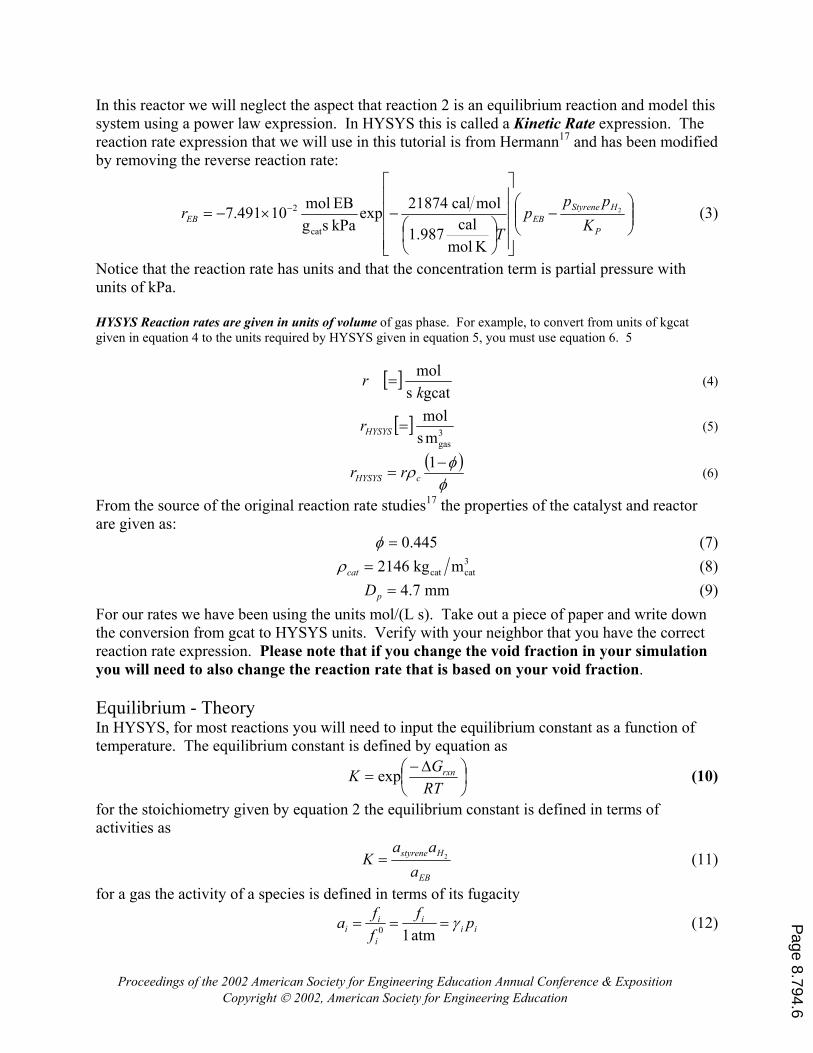
In this reactor we will neglect the aspect that reaction 2 is an equilibrium reaction and model this system using a power law expression. In HYSYS this is called a Kinetic Rate expression. The reaction rate expression that we will use in this tutorial is from Hermann17 and has been modified by removing the reverse reaction rate:

−

−×−= −

P

HStyreneEBEB K

ppp

Tr 2

K molcal1.987

molcal21874expkPa sgEB mol10491.7

cat

2 (3)

Notice that the reaction rate has units and that the concentration term is partial pressure with units of kPa. HYSYS Reaction rates are given in units of volume of gas phase. For example, to convert from units of kgcat given in equation 4 to the units required by HYSYS given in equation 5, you must use equation 6. 5

[ ]gcats

molk

r = (4)

[ ] 3gasms

mol=HYSYSr (5)

( )

φφρ −

=1

cHYSYS rr (6)

From the source of the original reaction rate studies17 the properties of the catalyst and reactor are given as: 445.0=φ (7) 3

catcat mkg2146=catρ (8) mm7.4=pD (9) For our rates we have been using the units mol/(L s). Take out a piece of paper and write down the conversion from gcat to HYSYS units. Verify with your neighbor that you have the correct reaction rate expression. Please note that if you change the void fraction in your simulation you will need to also change the reaction rate that is based on your void fraction. Equilibrium - Theory In HYSYS, for most reactions you will need to input the equilibrium constant as a function of temperature. The equilibrium constant is defined by equation as

∆−

=RTGK rxnexp (10)

for the stoichiometry given by equation 2 the equilibrium constant is defined in terms of activities as

EB

Hstyrene

aaa

K 2= (11)

for a gas the activity of a species is defined in terms of its fugacity

iii

i

ii pf

ffa γ===

atm 10 (12)


Page 8.794.6

where iγ has units of atm-1. Now combining equations 10, 11, and 12 results in the following for our stoichiometry given in equation 2,

atmexp

∆−

=RTGK rxn

P (13)

It is very important to note that the calculated value of Kp will have units and that the units are 1 atm, based on the standard states of gases. To predict as a function of temperature we will use the fully integrated van’t Hoff equation given in by Fogler18 in Appendix C as

rxnG∆

∆+

−

∆−∆=

R

p

R

pRT

oR

TP

TP

TT

RC

TTR

CTH

KK

R

R

lnˆ11

ˆln (14)

Now we can predict TPK as a function of temperature knowing only the heat of reaction at

standard conditions (usually 25°C and 1 atm and not STP!) and the heat capacity as a function of temperature. What is assumed in this equation is that all species are in one phase, either all gas or all vapor. For this Styrene reactor all of the species will be assumed to be in the gas phase and the following modification of equation 14 will be used

∆+

−

∆−∆=

R

vaporp

R

vaporpRT

vaporoR

TP

TP

TT

RC

TTRCTH

KK R

R

lnˆ11ˆ

ln (15)

The heat capacity term is defined as

( )R

T

T

vaporpvapor

p TT

TCC R

−=

∫ dˆ (16)

and for the above stoichiometry (17) vapor

pvaporp

vaporp

vaporp EBHstyrene

CCCC ˆˆˆˆ2

−+=∆

Now for some hand calculations! To determine the equilibrium conversion for this reaction we substitute equation 12 into equation 11 yielding

EB

HstyreneP p

ppK 2= (18)

Defining the conversion based on ethylbenzene (EB) and defining the partial pressure in terms of a molar flowrate gives:

( )

PFFF

PFFp

T

EBEBi

T

ii

χ00

−== (19)

Substituting equation 19 for each species into equation 18 with the feed stream consisting of no products and then simplifying gives

−=

EB

EBEB

TP

FFPK

χχ

1

20 (20)


Page 8.794.7

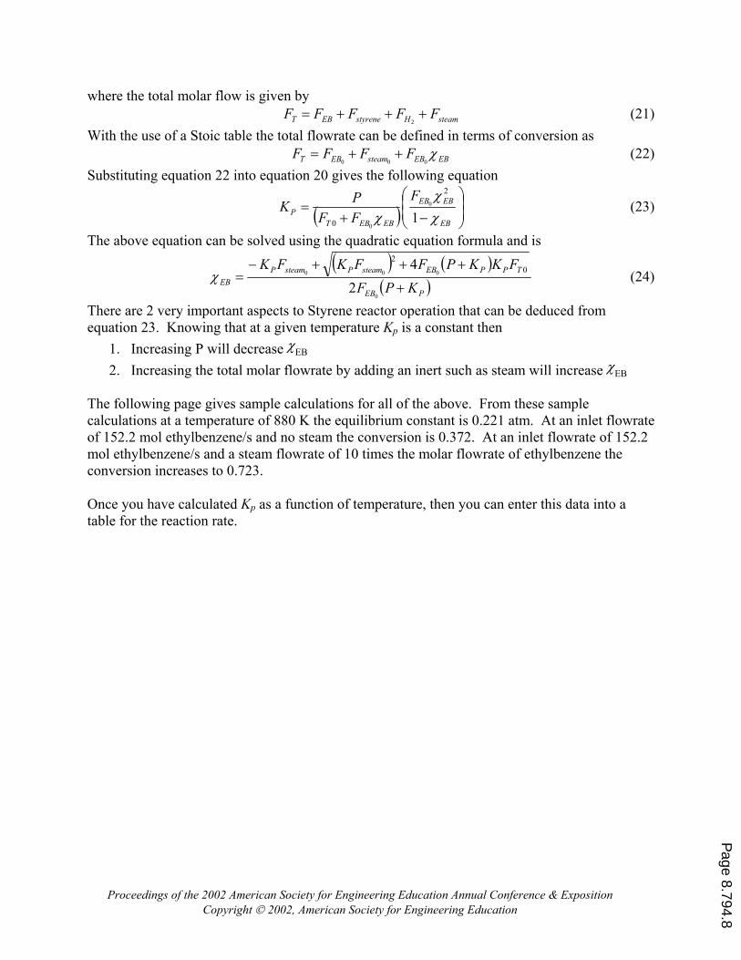
where the total molar flow is given by steamHstyreneEBT FFFFF +++=

2 (21)

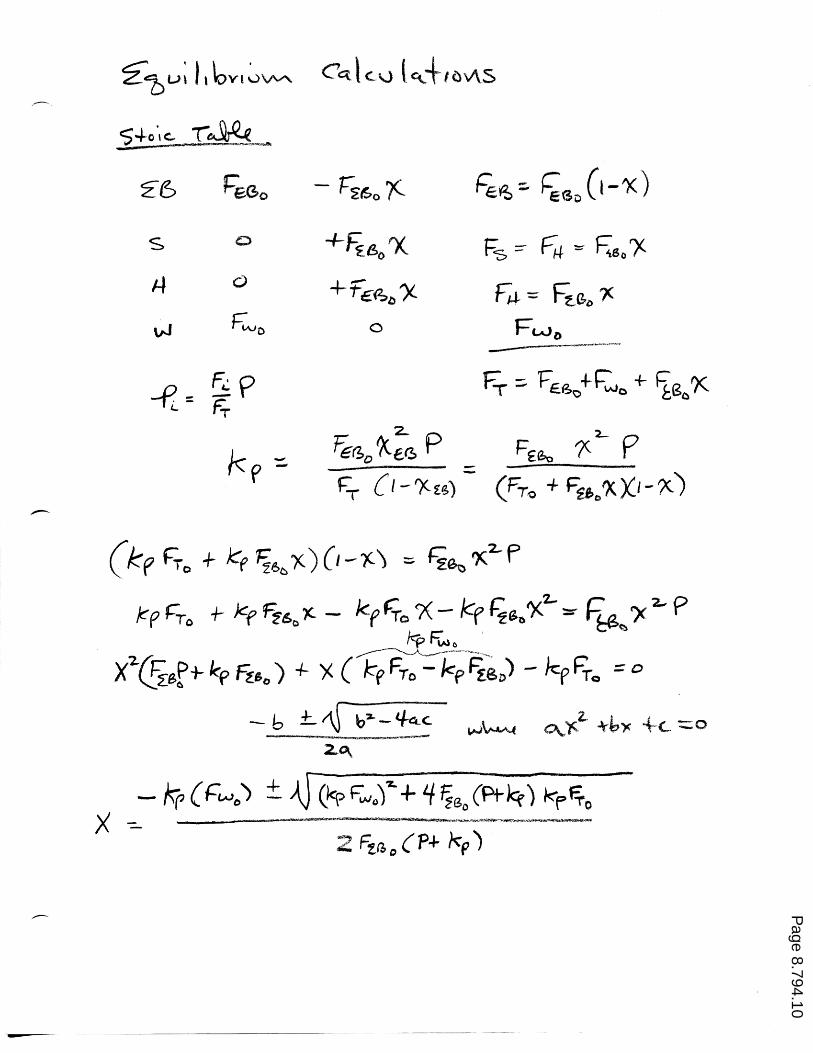
With the use of a Stoic table the total flowrate can be defined in terms of conversion as EBEBsteamEBT FFFF χ

000++= (22)

Substituting equation 22 into equation 20 gives the following equation

( )

−+=

EB

EBEB

EBEBTP

FFFPK

χχ

χ 1

2

0

0

0

(23)

The above equation can be solved using the quadratic equation formula and is

( ) ( )

( )PEB

TPPEBsteamPsteamPEB KPF

FKKPFFKFK+

+++−=

0

000

24 0

2

χ (24)

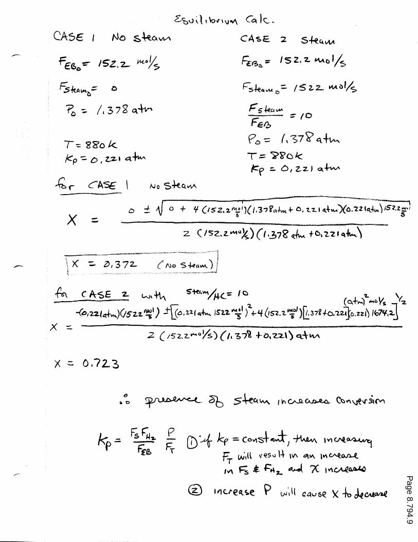
There are 2 very important aspects to Styrene reactor operation that can be deduced from equation 23. Knowing that at a given temperature Kp is a constant then

1. Increasing P will decrease χEB 2. Increasing the total molar flowrate by adding an inert such as steam will increase χEB

The following page gives sample calculations for all of the above. From these sample calculations at a temperature of 880 K the equilibrium constant is 0.221 atm. At an inlet flowrate of 152.2 mol ethylbenzene/s and no steam the conversion is 0.372. At an inlet flowrate of 152.2 mol ethylbenzene/s and a steam flowrate of 10 times the molar flowrate of ethylbenzene the conversion increases to 0.723. Once you have calculated Kp as a function of temperature, then you can enter this data into a table for the reaction rate.


.794.8

794.10

Press here to add components

Press here to start adding rxns

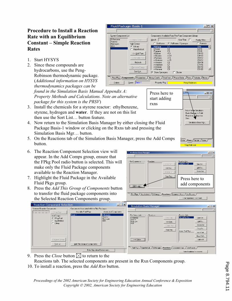
Procedure to Install a Reaction Rate with an Equilibrium Constant – Simple Reaction Rates 1. Start HYSYS 2. Since these compounds are

hydrocarbons, use the Peng-Robinson thermodynamic package. (Additional information on HYSYS thermodynamics packages can be found in the Simulation Basis Manual Appendix A: Property Methods and Calculations. Note an alternative package for this system is the PRSV)

3. Install the chemicals for a styrene reactor: ethylbenzene, styrene, hydrogen and water. If they are not on this list then use the Sort List… button feature.

4. Now return to the Simulation Basis Manager by either closing the Fluid Package Basis-1 window or clicking on the Rxns tab and pressing the Simulation Basis Mgr… button.

5. On the Reactions tab of the Simulation Basis Manager, press the Add Comps button.

6. The Reaction Component Selection view will appear. In the Add Comps group, ensure that the FPkg Pool radio button is selected. This will make only the Fluid Package components available to the Reaction Manager.

7. Highlight the Fluid Package in the Available Fluid Pkgs group.

8. Press the Add This Group of Components button to transfer the fluid package components into

Press the Close button

the Selected Reaction Components group.

9. to return to the Reactions tab. The selected components are present in the Rxn Components group. To install a reaction, press the Ad10. d Rxn button.


Page 8.794.11

ponent as ethylbenzene and

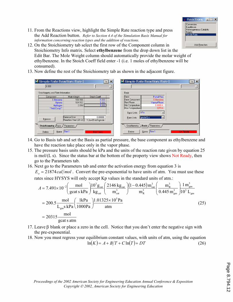
11. From the Reactions view, highlight the Simple Rate reaction type and press

12. nent column in the

ght of

13. Now define the rest of the Stoichiometry tab as shown in the adjacent figure.

15. The pressure basis units should be kPa and the units of the reaction rate given by equation 25

16. b and enter the activation energy from equation 3 is

the Add Reaction button. Refer to Section 4.4 of the Simulation Basis Manual for information concerning reaction types and the addition of reactions. On the Stoichiometry tab select the first row of the CompoStoichiometry Info matrix. Select ethylbenzene from the drop down list inEdit Bar. The Mole Weight column should automatically provide the molar weiethylbenzene. In the Stoich Coeff field enter -1 (i.e. 1 moles of ethylbenzene will be consumed).

14. Go to Basis tab and set the Basis as partial pressure, the base comhave the reaction take place only in the vapor phase.

is mol/(L s). Since the status bar at the bottom of the property view shows Not Ready, then go to the Parameters tab. Next go to the Parameters ta

molcalEa 21874= . Convert the pre-exponential to have units of atm. You muill only accept Kp values in the standard units of atm.:

( ) mm 445.01kg 2146g10mol 333 −−

st use these rates since HYSYS w

atm sgcat mol20315

atmPa1001325.1

Pa1000kPa1

kPa sLmol5.200

L 10m 1

m 0.445mmkgkPa sgcat 10491.7

5

gas

gas3

3gas

3gas

R3R

cat3cat

cat

cat

cat2

=

×

=

×=A

(25)

17. Leave β blank or place a zero in the cell. Notice that you don’t enter the negative sign with

18. your equilibrium constant values, with units of atm, using the equation the pre-exponential. Now you must regress

( ) ( ) DTTCTBAK +++= lnln (26)


Page 8.794.12

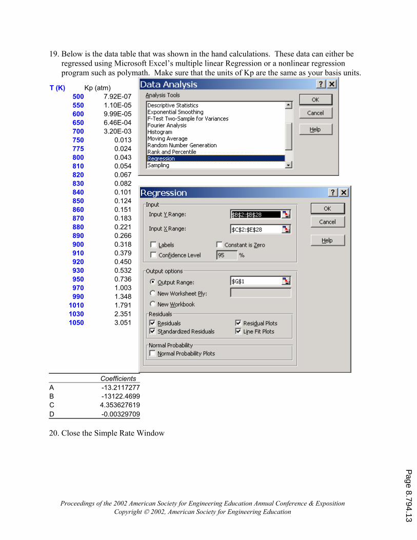
19. Below is the data table that was shown in the hand calculations. These data can either be regressed using Microsoft Excel’s multiple linear Regression or a nonlinear regression program such as polymath. Make sure that the units of Kp are the same as your basis units.

T (K) Kp (atm) 500 7.92E-07550 1.10E-05600 9.99E-05650 6.46E-04700 3.20E-03750 0.013775 0.024800 0.043810 0.054820 0.067830 0.082840 0.101850 0.124860 0.151870 0.183880 0.221890 0.266900 0.318910 0.379920 0.450930 0.532950 0.736970 1.003990 1.348

1010 1.7911030 2.3511050 3.051

Coefficients A -13.2117277B -13122.4699C 4.353627619D -0.00329709 20. Close the Simple Rate Window


Page 8.794.13

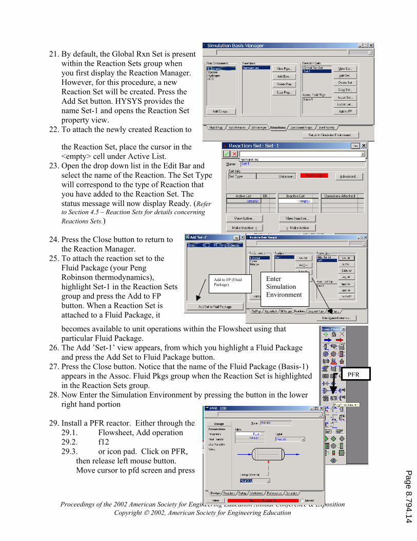
21. By default, the Global Rxn Set is present within the Reaction Sets group when you first display the Reaction Manager. However, for this procedure, a new Reaction Set will be created. Press the Add Set button. HYSYS provides the name Set-1 and opens the Reaction Set property view.

22. To attach the newly created Reaction to

the Reaction Set, place the cursor in the <empty> cell under Active List.

23. Open the drop down list in the Edit Bar and select the name of the Reaction. The Set Type will correspond to the type of Reaction that you have added to the Reaction Set. The status message will now display Ready. (Rto Section 4.5 – Reaction Sets for details concerninReactions Sets.)

efer g

PFR

lowsheet using that

Enter Simulation Environment

Add to FP (Fluid Package)

24. Press the Close button to return to

25. To attach the reaction set to the

ets

26. ighlight a Fluid Package

27.kgs group when the Reaction Set is highlighted

28. lation Environment by pressing the button in the lower right hand portion

29. Install a PFR reactor. Either through the , Add operation

29.3 ,

the Reaction Manager.

Fluid Package (your Peng Robinson thermodynamics), highlight Set-1 in the Reaction Sgroup and press the Add to FP button. When a Reaction Set is attached to a Fluid Package, it

becomes available to unit operations within the Fparticular Fluid Package. The Add ’Set-1’ view appears, from which you hand press the Add Set to Fluid Package button. Press the Close button. Notice that the name of the Fluid Package (Basis-1) appears in the Assoc. Fluid Pin the Reaction Sets group. Now Enter the Simu

29.1. Flowsheet29.2. f12

. or icon pad. Click on PFRthen release left mouse button. Move cursor to pfd screen and press


Page 8.794.14

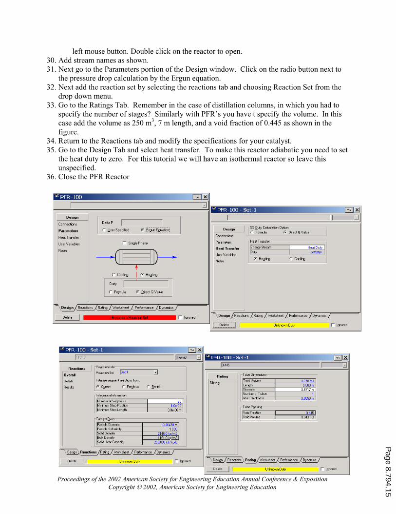
left mouse button. Double click on the reactor to open.

31. w. Click on the radio button next to

32. Next add the reaction set by selecting the reactions tab and choosing Reaction Set from the

33.is

the volume as 250 m3, 7 m length, and a void fraction of 0.445 as shown in the

35. to set o zero. For this tutorial we will have an isothermal reactor so leave this

36. Close the PFR Reactor

30. Add stream names as shown. Next go to the Parameters portion of the Design windothe pressure drop calculation by the Ergun equation.

drop down menu. Go to the Ratings Tab. Remember in the case of distillation columns, in which you had to specify the number of stages? Similarly with PFR’s you have t specify the volume. In thcase add figure.

34. Return to the Reactions tab and modify the specifications for your catalyst. Go to the Design Tab and select heat transfer. To make this reactor adiabatic you needthe heat duty tunspecified.


Page 8.794.15

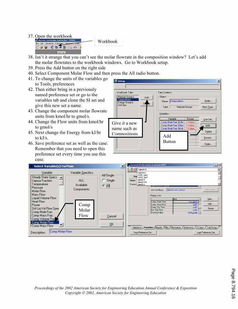
37. Open the workbook

38. Isn’t it strange that you can’t see the molar flowrate in the composition window? Let’s add

the molar flowrates to the workbook windows. Go to Workbook setup. 39. Press the Add button on the right side 40. Select Component Molar Flow and then press the All radio button. 41. To change the units of the variables go

to Tools, preferences 42. Then either bring in a previously

named preference set or go to the variables tab and clone the SI set and give this new set a name.

Button

43. Change the component molar flowrate units from kmol/hr to gmol/s.

44. Change the Flow units from kmol/hr to gmol/s

Give it a new name such as Compositions45. Next change the Energy from kJ/hr

to kJ/s. Add 46. Save preference set as well as the case.

Remember that you need to open this preference set every time you use this case.

Workbook

Comp Molar Flow


Page 8.794.16

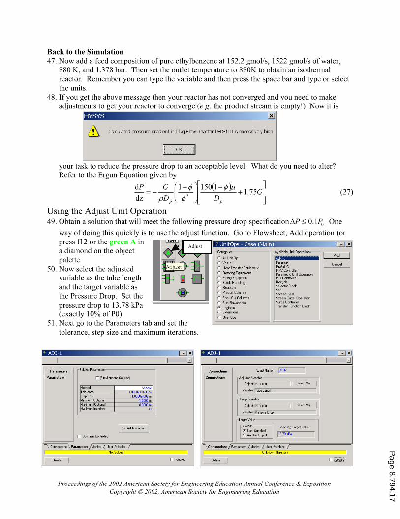
Back to the Simulation 47. Now add a feed composition of pure ethylbenzene at 152.2 gmol/s, 1522 gmol/s of water,

880 K, and 1.378 bar. Then set the outlet temperature to 880K to obtain an isothermal reactor. Remember you can type the variable and then press the space bar and type or select the units.

48. If you get the above message then your reactor has not converged and you need to make

your task to reduce the pressure drop to an acceptable level. What do you need to alter? Refer to the Ergun Equation given by

GP 1d

adjustments to get your reactor to converge (e.g. the product stream is empty!) Now it is

( )

+

−

−−= G

DD pp

75.11150dz 3

µφφ

φρ

Adjust

01.0 PP ≤∆way of doing this quickly is to use the adjust function. Go to Flowsheet, A ion (orpress f12 or the green A in a diamond on the object palette.

(27)

Using the Adjust Unit Operation following pressure drop specification One

dd operat

50. Now select the adjusted h

51.s.

49. Obtain a solution that will meet the

variable as the tube lengtand the target variable as the Pressure Drop. Set thepressure drop to 13.78 kPa (exactly 10% of P0). Next go to the Parameters tab and set the tolerance, step size and maximum iteration


Page 8.794.17

Proceedings of the 2002 American Society for EngiCopyright 2002, American Society

neering Education Annual Conference & Exposition for Engineering Education

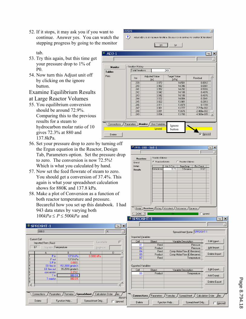
52. If it stops, it may ask you if you want to continue. Answer yes. You can watch the stepping progress by going to the monitor

tab. 53. Try this again, but this time get

your pressure drop to 1% of P0.

54. Now turn this Adjust unit off by clicking on the ignore button.

Examine Equilibrium Results at Large Reactor Volumes 55. You equilibrium conversion

should be around 72.9%. Comparing this to the previous results for a steam to hydrocarbon molar ratio of 10 gives 72.3% at 880 and 137.8kPa.

Ignore button

56. Set your pressure drop to zero by turning off the Ergun equation in the Reactor, Design Tab, Parameters option. Set the pressure drop to zero. The conversion is now 72.5%! Which is what you calculated by hand.

57. Now set the feed flowrate of steam to zero. You should get a conversion of 37.4%. This again is what your spreadsheet calculation shows for 880K and 137.8 kPa.

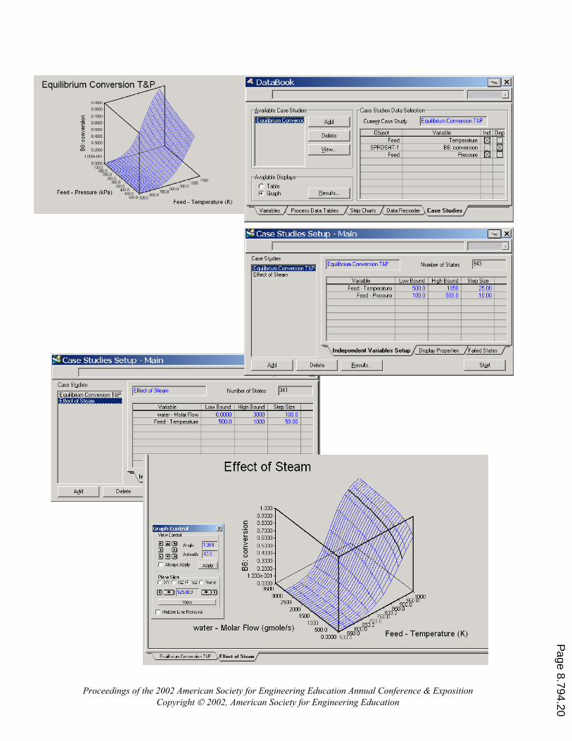
58. Make a plot of Conversion as a function of both reactor temperature and pressure. Becareful how you set up this databook. I had 943 data states by varying both

kPaPkPa 500100 ≤≤ and

Page 8.794.18


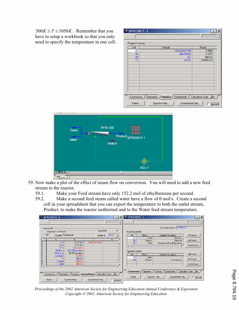
R ber that you have to setup a workbook so that you only

eed stream have only 152.2 mol of ethylbenzene per second. cond

KTK 1050500 ≤≤ .

59. Now ma

emem

need to specify the temperature in one cell.

ke a plot of the effect of steam flow on conversion. You will need to add a new feed stream to the reactor. 59.1. Make your F59.2. Make a second feed steam called water have a flow of 0 mol/s. Create a se

cell in your spreadsheet that you can export the temperature to both the outlet stream, Product, to make the reactor isothermal and to the Water feed stream temperature.

Page 8.794.19


Page 8.794.20

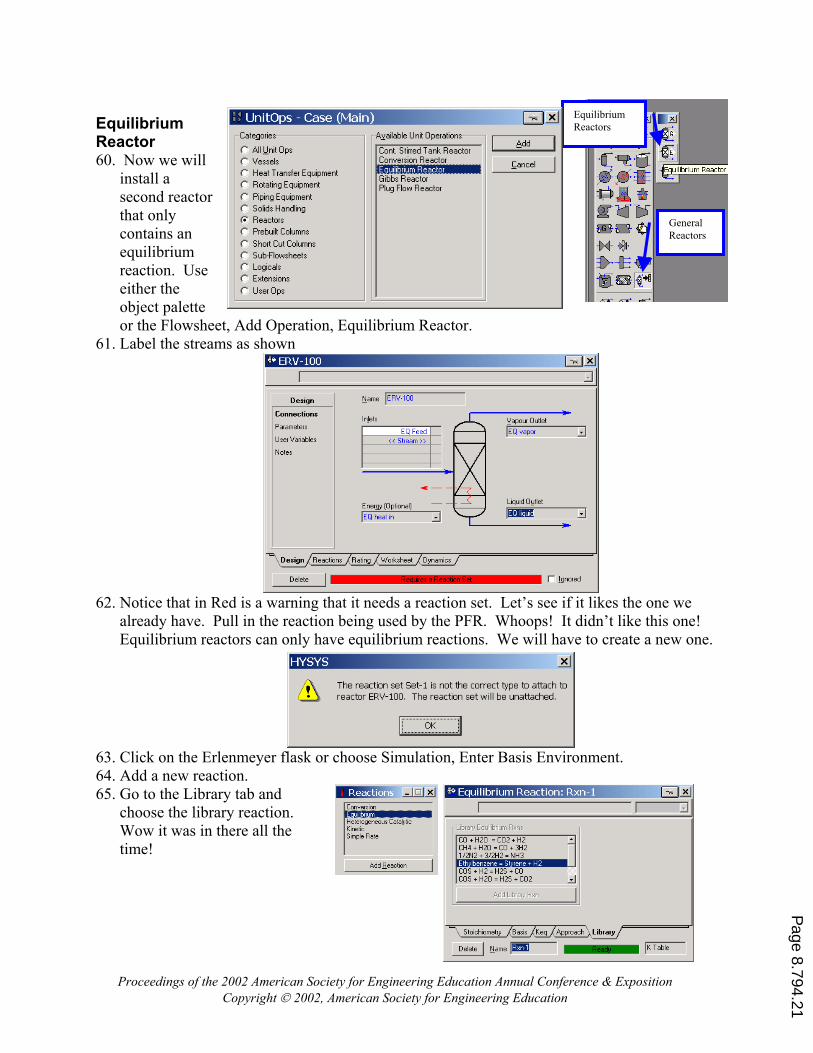
Equilibrium Reactors

neering Education Annual Conference & 2002, American Society for Engineering Education

Exposition Copyright

General Reactors

Equilibrium Reactor 60. Now we will

install a second reactor that only contains an equilibrium reaction. Use either the object palette or the Flowsheet, Add Operation, Equilibrium Reactor.

61. Label the streams as shown

ng that it needs a reaction set. Let’s see if it likes the one we

63. k or 64. Add a new reaction. 65. Go to the Library tab and

choose the library reaction. Wow it was in there all the time!

62. Notice that in Red is a warnialready have. Pull in the reaction being used by the PFR. Whoops! It didn’t like this one!Equilibrium reactors can only have equilibrium reactions. We will have to create a new one.

Click on the Erlenmeyer flas choose Simulation, Enter Basis Environment.

Proceedings of the 2002 American Society for Engi

Page 8.794.21

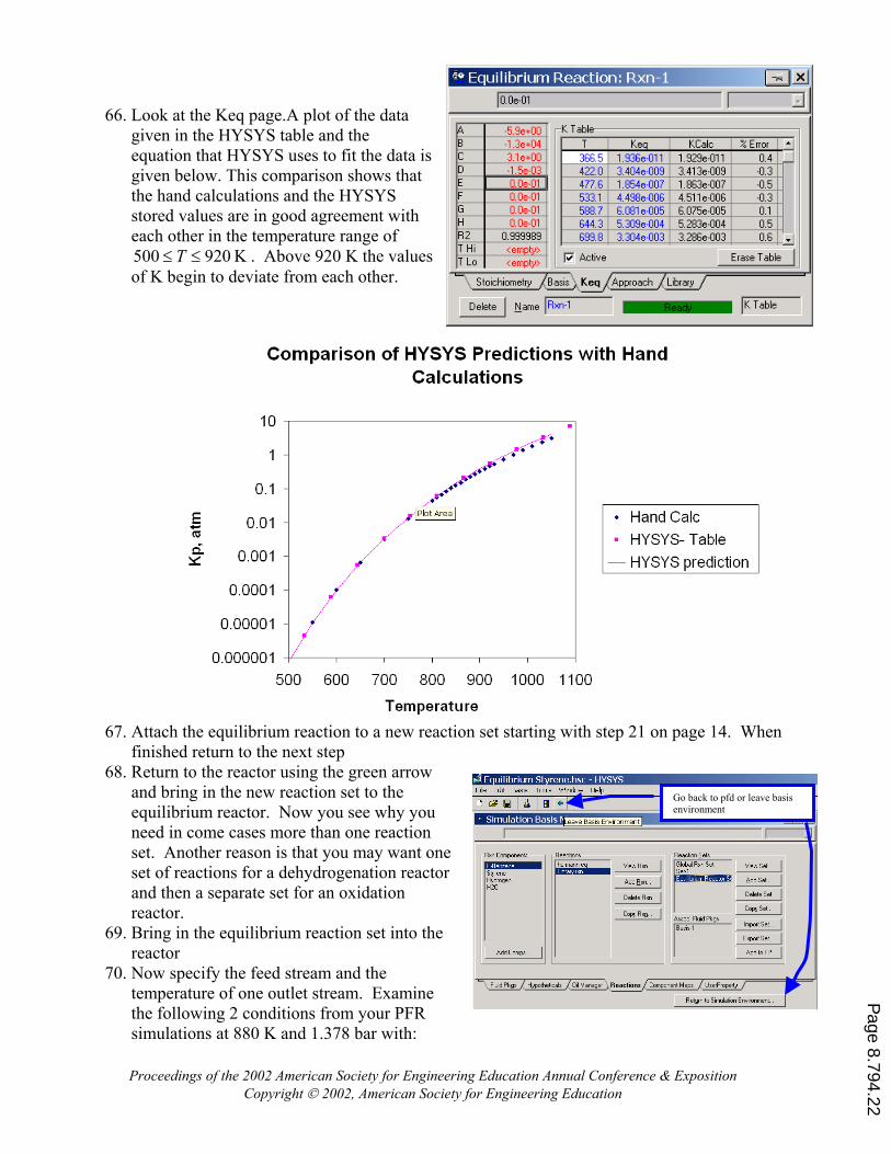
66. Look at the Keq page.A plot of the data given in the HYSYS table and the equation that HYSYS uses to fit the data is given below. This comparison shows that the hand calculations and the HYSYS stored values are in good agreement with each other in the temperature range of

. Above 920 K the vof K begin to deviate from each other.

K 920500 ≤≤ T alues

Go back to pfd or leave basis environment

67. Attach the equilibrium reaction to a new reaction set starting with step 21 on page 14. When

68. Return to the reactor using the green arrow

ou

e

69. Bring in the equilibrium reaction set into the

70. Now specify the feed stream and the mine

finished return to the next step

and bring in the new reaction set to the equilibrium reactor. Now you see why yneed in come cases more than one reaction set. Another reason is that you may want onset of reactions for a dehydrogenation reactor and then a separate set for an oxidation reactor.

reactor

temperature of one outlet stream. Exathe following 2 conditions from your PFR simulations at 880 K and 1.378 bar with:


Page 8.794.22

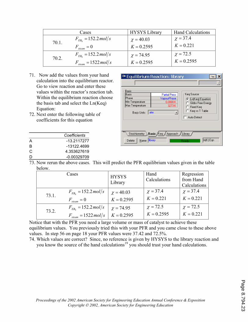
Cases HYSYS Library Hand Calculations

70.1. 0

2.

=steam

E

F

smolF

1520

=B

2595.0=03.40=

Kχ

221.0=K4.37=χ

smolF

smolF

steam

EB

1522

2.1520

=

=

2595.095.74

==

Kχ

2595.05.72

==

Kχ

70.2.

1. Now add the values from your hand

r.

ab.

72. Next enter the following table of

Coefficients

7calculation into the equilibrium reactoGo to view reaction and enter these values within the reactor’s reaction tWithin the equilibrium reaction choose the basis tab and select the Ln(Keq) Equation:

coefficients for this equation

A -13.2117277B -13122.4699C 4.353627619D -0.0032970973. Now rerun the This will predict the PFR equilibrium values given in the table

Cases HYSYS Hand ations

Regression

above cases.below.

Library Calcul from Hand Calculations

0

2.1520

=

=

steam

EB

F

smolF

2595.003.40

==

Kχ

221.04.37

==

Kχ

221.0=K4.37=χ

smolF

smolF

steam

EB

1522

2.1520

=

=

2595.095.74

==

Kχ

2595.05.72

==

Kχ

221.05.72

==

Kχ

73.1.

73.2.

Notice that with the PFR you need a large volume or mass of catalyst to achieve these se above

the library reaction and

equilibrium values. You previously tried this with your PFR and you came close to thevalues. In step 56 on page 18 your PFR values were 37.42 and 72.5%. 74. Which values are correct? Since, no reference is given by HYSYS to

you know the source of the hand calculations19 you should trust your hand calculations.


Page 8.794.23

View Component

Minimization of Gibbs Free Energy 75. Go back to the reaction screen and choose the

Gibbs Free Energy radio button. 76. Wow! Now you get 100% conversion. Please note

that this problem does not exist in HYSYS version 3.0 and later. Why is this and what is going on? If you change the reactor temperature to about 510 K then you obtain 37% conversion for the case with no water. In this calculation, the equilibrium constant is determined from the Ideal Gas Gibbs Free Energy Coefficients in the HYSYS library.

77. Examine these values. 77.1. Enter the basis environment. 77.2. View the property package 77.3. Select styrene and view the

component 77.4. Choose the

temperature dependent tab: Tdep. Notice that the default values for the Ideal Gas Gibbs Free Energy Coefficients in the HYSYS library are not temperature dependent. It is a constant. This is incorrect. The correct values are given in the cloned component created by Aaron Pollock of Hyprotech Technical Support.20 This is a clear eof why you can’ttrust a process simulator to give you the correct values. You neeto investigatewhat it is doing. Please notethis problem does not exist HYSYS version 3.0 and later.

xample

d

that

in


Page 8.794.24

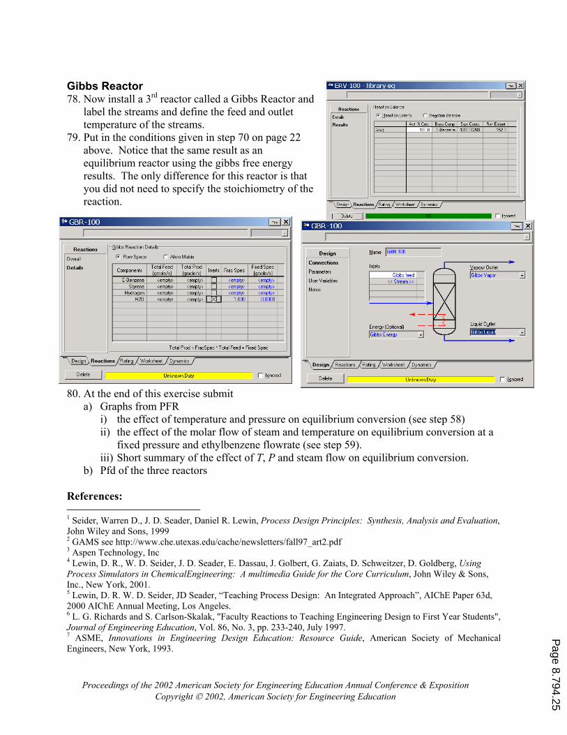
Gibbs Reactor 78. Now install a 3rd reactor called a Gibbs Reactor and

label the streams and define the feed and outlet temperature of the streams.

79. Put in the conditions given in step 70 on page 22 above. Notice that the same result as an equilibrium reactor using the gibbs free energy results. The only difference for this reactor is that you did not need to specify the stoichiometry of the reaction.

80. At the end of this exercise submit a) Graphs from PFR

i) the effect of temperature and pressure on equilibrium conversion (see step 58) ii) the effect of the molar flow of steam and temperature on equilibrium conversion at a

fixed pressure and ethylbenzene flowrate (see step 59). iii) Short summary of the effect of T, P and steam flow on equilibrium conversion.

b) Pfd of the three reactors References: 1 Seider, Warren D., J. D. Seader, Daniel R. Lewin, Process Design Principles: Synthesis, Analysis and Evaluation, John Wiley and Sons, 1999 2 GAMS see http://www.che.utexas.edu/cache/newsletters/fall97_art2.pdf 3 Aspen Technology, Inc 4 Lewin, D. R., W. D. Seider, J. D. Seader, E. Dassau, J. Golbert, G. Zaiats, D. Schweitzer, D. Goldberg, Using Process Simulators in ChemicalEngineering: A multimedia Guide for the Core Curriculum, John Wiley & Sons, Inc., New York, 2001. 5 Lewin, D. R. W. D. Seider, JD Seader, “Teaching Process Design: An Integrated Approach”, AIChE Paper 63d, 2000 AIChE Annual Meeting, Los Angeles. 6 L. G. Richards and S. Carlson-Skalak, "Faculty Reactions to Teaching Engineering Design to First Year Students", Journal of Engineering Education, Vol. 86, No. 3, pp. 233-240, July 1997. 7 ASME, Innovations in Engineering Design Education: Resource Guide, American Society of Mechanical Engineers, New York, 1993.


Page 8.794.25

8 R. H. King, T. E. Parker, T. P. Grover, J. P. Gosink, N. T. Middleton, "A Multidisciplinary Engineering Laboratory Course", Journal of Engineering Education, Vol. 88, No. 3, pp. 311-316, July 1999. 9 S. S. Courter, S. B. Millar and L. Lyons, "From the Student's Point of View: Experiences in a Freshman Engineering Design Course", Journal of Engineering Education, Vol. 87, No. 3, pp. 283-288, July 1998. 10 "Engineering Criteria 2000: Criteria for Accrediting Programs in Engineering in the United States," 3rd Ed., Engineering Accreditation Commission, Accreditation Board for Engineering and Technology, Inc., Baltimore, MD, 1999, http://www.abet.org/eac/eac.htm. 11 Phillip C. Wankat, Equilibrium Staged Separations, Elsevier, 1988. 12 Michael A. Henson and Yougchun Zhang, “Integration pf Commercial Dynamic Simulators into the Undergraduate Process Control Curriculum”. Proceedings of the AIChE Annual Meeting, Los Angeles, CA, Nov. 2000. 13 David E. Clough, “ Using Process Simulators with Dynamics/Control Capabilities to Teach Unit and Plantwide Control Strategies”. Proceedings of the AIChE Annual Meeting, Los Angeles, CA, Nov. 2000. 14 A. S. Foss, K. R. Guerts, P. J. Goodeve, K. D. Dahm, G. Stephanopoulos, J. Bieszczad, A. Koulouris, "A Phenomena-Oriented Environment for Teaching Process Modeling: Novel Modeling Software and Its Use in Problem Solving," Chemical Engineering Education, Fall 1999. 15 Fogler, H. Scott, Elements of Chemical Reaction Engineering, 3rd Ed., Prentice Hall PTR, Upper Saddle River, NJ, 1999. 16 R. P. Hesketh, “Incorporating Reactor Design Projects into the Course,” Paper 149e, 1999 AIChE Annual Meeting, Dallas, TX, 31 October - 5 November 1999. 17 Hermann, Ch.; Quicker, P.; Dittmeyer, R., “Mathematical simulation of catalytic dehydrogenation of ethylbenzene to styrene in a composite palladium membrane reactor.” J. Membr. Sci. (1997), 136(1-2), 161-172. 18 Fogler, H. S. Elements of Chemical Reaction Engineering, 3rd Ed., by, Prentice Hall PTR, Englewood Cliffs, NJ (1999). 19 "Thermodynamics Source Database" by Thermodynamics Research Center, NIST Boulder Laboratories, M. Frenkel director, in NIST Chemistry WebBook, NIST Standard Reference Database Number 69, Eds. P.J. Linstrom and W.G. Mallard, July 2001, National Institute of Standards and Technology, Gaithersburg MD, 20899 (http://webbook.nist.gov). 20 Yaws, C.L. and Chiang, P.Y., "Find Favorable Reactions Faster", Hydrocarbon Processing, November 1988, pg 81-84.

BIOGRAPHICAL INFORMATION

Stephanie Farrell is Associate Professor of Chemical Engineering at Rowan University. She received her B.S. in 1986 from the University of Pennsylvania, her MS in 1992 from Stevens Institute of Technology, and her Ph.D. in 1996 from New Jersey Institute of Technology. Prior to joining Rowan in September 1998, she was a faculty member in Chemical Engineering at Louisiana Tech University. Stephanie’s has research expertise in the field of drug delivery, and integrates pharmaceutical and biomedical topics and experiments into the chemical engineering curriculum. Stephanie won the 2000 Dow Outstanding Young Faculty Award, the 2001 Joseph J. Martin Award, and the 2002 Ray W. Fahien Award.

Robert Hesketh is a highly motivated professor in both undergraduate and graduate education and has received 9 education and 2 research awards, including ASEE’s 1999 Ray W. Fahien Award. He has made major contributions in laboratory methods that demonstrate chemical engineering practice and principles. These highly visual and effective experiments, the most notable using the vehicle of a coffeemaker, are used to introduce engineering design and science to university and pre-college students. He has developed over 20 experiments employed throughout the curriculum at Rowan University. These experiments range from small scale coffee experiments to 25 ft distillation column experiments. His work has been presented at national meetings, workshops and published in journals and proceedings and his experiments are being used in over 15 institutions. He has attracted over 2 million dollars in external funding for research and educational activities.


Page 8.794.26

C. Stewart Slater is Professor and Chair of Chemical Engineering at Rowan University. He received his B.S., M.S. and Ph.D. from Rutgers University. Prior to joining Rowan he was Professor of Chemical Engineering at Manhattan College where he was active in chemical engineering curriculum development and established a laboratory for advanced separation processes with the support of the National Science Foundation and industry. Dr. Slater's research and teaching interests are in separation and purification technology, laboratory development, and investigating novel processes for interdisciplinary fields such as biotechnology and environmental engineering. He has authored over 70 papers and several book chapters. Dr. Slater has been active in ASEE, having served as Program Chair and Director of the Chemical Engineering Division and has held every office in the DELOS Division. Dr. Slater has received numerous national awards including the 1999 and 1998 Joseph J. Martin Award, 1999 Chester Carslon Award, 1996 George Westinghouse Award, 1992 John Fluke Award, 1992 DELOS Best Paper Award and 1989 Dow Outstanding Young Faculty Award.


Page 8.794.27

issues encountered with students using process … · session 2003-2484 issues encountered w ith...

Documents