issn 2380-3525 (print) critical reviewfs.unm.edu/criticalreview-12-2016.pdf5 critical review. volume...
TRANSCRIPT

Critical Review
A Publication of Society for Mathematics of Uncertainty
Editors:
Paul P. Wang
John N. Mordeson
Mark J. Wierman
Volume XII, 2016
Publisher:
Center for Mathematics of Uncertainty
Creighton University
ISSN 2380-3525 (Print)ISSN 2380-3517 (Online)

Critical Review A Publication of Society for Mathematics of Uncertainty
Volume XII, 2016
Editors:
Paul P. Wang
John N. Mordeson
Mark J. Wierman
Publisher:
Center for Mathematics of Uncertainty
Creighton University
We devote part of this issue of Critical Review to Lotfi Zadeh.
The Editors.
Paul P. Wang Department of Electrical and Computer Engineering Pratt School of Engineering Duke University Durham, NC 27708-0271 [email protected]
John N. Mordeson Department of Mathematics Creighton University Omaha, Nebraska 68178 [email protected]
Mark J. Wierman Department of Journalism Media & Computing Creighton University Omaha, Nebraska 68178 [email protected]

Contents
S. Broumi, M. Talea, A. Bakali, F. Smarandache
Interval Valued Neutrosophic Graphs
A. Salama, F. Smarandache
Neutrosophic Crisp Probability Theory & Decision Making Process
S. Broumi, M. Talea, A. Bakali, F. Smarandache
On Strong Interval Valued Neutrosophic Graphs
F. Smarandache, H. E. Khalid, A. K. Essa, M. Ali
The Concept of Neutrosophic Less than or Equal: A New Insight in
Unconstrained Geometric Programming
A. Elhassouny, F. Smarandache
Multi-Criteria Decision Making Method for n-wise Criteria Comparisons and
Inconsistent Problems
5
34
49
72
81


5
Critical Review. Volume X, 2016
Interval Valued Neutrosophic Graphs
Said Broumi1, Mohamed Talea2, Assia Bakali3,
Florentin Smarandache4
1,2 Laboratory of Information Processing, Faculty of Science Ben M’Sik, University Hassan II,
B.P 7955, Sidi Othman, Casablanca, Morocco [email protected], [email protected]
3 Ecole Royale Navale, Boulevard Sour Jdid, B.P 16303 Casablanca, Morocco
4 Department of Mathematics, University of New Mexico, 705 Gurley Avenue,
Gallup, NM 87301, USA
Abstract
The notion of interval valued neutrosophic sets is a generalization of fuzzy sets,
intuitionistic fuzzy sets, interval valued fuzzy sets, interval valued intuitionstic fuzzy
sets and single valued neutrosophic sets. We apply for the first time to graph theory
the concept of interval valued neutrosophic sets, an instance of neutrosophic sets. We
introduce certain types of interval valued neutrosophc graphs (IVNG) and investigate
some of their properties with proofs and examples.
Keyword
Interval valued neutrosophic set, Interval valued neutrosophic graph, Strong interval
valued neutrosophic graph, Constant interval valued neutrosophic graph, Complete
interval valued neutrosophic graph, Degree of interval valued neutrosophic graph.
1 Introduction
Neutrosophic sets (NSs) proposed by Smarandache [13, 14] are powerful
mathematical tools for dealing with incomplete, indeterminate and
inconsistent information in real world. They are a generalization of fuzzy sets
[31], intuitionistic fuzzy sets [28, 30], interval valued fuzzy set [23] and
interval-valued intuitionistic fuzzy sets theories [29].
The neutrosophic sets are characterized by a truth-membership function (t),
an indeterminacy-membership function (i) and a falsity-membership function
(f) independently, which are within the real standard or nonstandard unit
interval ]−0, 1+[. In order to conveniently practice NS in real life applications,
Smarandache [53] and Wang et al. [17] introduced the concept of single-valued
neutrosophic set (SVNS), a subclass of the neutrosophic sets.

6
Said Broumi, Mohamed Talea, Assia Bakali, Florentin Smarandache
Interval Valued Neutrosophic Graphs
Critical Review. Volume XII, 2016
The same authors [16, 18] introduced as well the concept of interval valued
neutrosophic set (IVNS), which is more precise and flexible than the single
valued neutrosophic set. The IVNS is a generalization of the single valued
neutrosophic set, in which three membership functions are independent, and
their values included into the unit interval [0, 1].
More on single valued neutrosophic sets, interval valued neutrosophic sets
and their applications may be found in [3, 4, 5,6, 19, 20, 21, 22, 24, 25, 26, 27,
39, 41, 42, 43, 44, 45, 49].
Graph theory has now become a major branch of applied mathematics and it
is generally regarded as a branch of combinatorics. Graph is a widely used tool
for solving a combinatorial problem in different areas, such as geometry,
algebra, number theory, topology, optimization or computer science. Most
important thing which is to be noted is that, when we have uncertainty
regarding either the set of vertices or edges, or both, the model becomes a
fuzzy graph.
The extension of fuzzy graph [7, 9, 38] theory have been developed by several
researchers, including intuitionistic fuzzy graphs [8, 32, 40], considering the
vertex sets and edge sets as intuitionistic fuzzy sets. In interval valued fuzzy
graphs [33, 34], the vertex sets and edge sets are considered as interval valued
fuzzy sets. In interval valued intuitionstic fuzzy graphs [2, 48], the vertex sets
and edge sets are regarded as interval valued intuitionstic fuzzy sets. In bipolar
fuzzy graphs [35, 36], the vertex sets and edge sets are considered as bipolar
fuzzy sets. In m-polar fuzzy graphs [37], the vertex sets and edge sets are
regarded as m-polar fuzzy sets.
But, when the relations between nodes (or vertices) in problems are
indeterminate, the fuzzy graphs and their extensions fail. In order to overcome
the failure, Smarandache [10, 11, 12, 51] defined four main categories of
neutrosophic graphs: I-edge neutrosophic graph, I-vertex neutrosophic graph
[1, 15, 50, 52], (t, i, f)-edge neutrosophic graph and (t, i, f)-vertex neutrosophic
graph. Later on, Broumi et al. [47] introduced another neutrosophic graph
model. This model allows the attachment of truth-membership (t),
indeterminacy –membership (i) and falsity-membership (f) degrees both to
vertices and edges. A neutrosophic graph model that generalizes the fuzzy
graph and intuitionstic fuzzy graph is called single valued neutrosophic graph
(SVNG). Broumi [46] introduced as well the neighborhood degree of a vertex
and closed neighborhood degree of a vertex in single valued neutrosophic
graph, as generalizations of neighborhood degree of a vertex and closed
neighborhood degree of a vertex in fuzzy graph and intuitionistic fuzzy graph.
In this paper, we focus on the study of interval valued neutrosophic graphs.

7
Critical Review. Volume XII, 2016
Said Broumi, Mohamed Talea, Assia Bakali, Florentin Smarandache .
Interval Valued Neutrosophic Graphs
2 Preliminaries
In this section, we mainly recall some notions related to neutrosophic sets,
single valued neutrosophic sets, interval valued neutrosophic sets, fuzzy graph,
intuitionistic fuzzy graph, single valued neutrosophic graphs, relevant to the
present work. See especially [2, 7, 8, 13, 18, 47] for further details and
background.
Definition 2.1 [13]
Let X be a space of points (objects) with generic elements in X denoted by x;
then the neutrosophic set A (NS A) is an object having the form A = {< x: TA(x),
IA(x), FA(x)>, x ∈ X}, where the functions T, I, F: X→]−0,1+[ define respectively
the a truth-membership function, an indeterminacy-membership function,
and a falsity-membership function of the element x ∈ X to the set A with the
condition:
−0 ≤ TA(x)+ IA(x)+ FA(x)≤ 3+.
The functions TA(x), IA(x) and FA(x) are real standard or nonstandard subsets
of ]−0,1+[.
Since it is difficult to apply NSs to practical problems, Wang et al. [16]
introduced the concept of a SVNS, which is an instance of a NS and can be used
in real scientific and engineering applications.
Definition 2.2 [17]
Let X be a space of points (objects) with generic elements in X denoted by x. A
single valued neutrosophic set A (SVNS A) is characterized by truth-
membership function TA(x) , an indeterminacy-membership function IA(x) ,
and a falsity-membership function FA(x). For each point x in X TA(x), IA(x),
FA(x) ∈ [0, 1]. A SVNS A can be written as
A = {< x: TA(x), IA(x), FA(x)>, x ∈ X}
Definition 2.3 [7]
A fuzzy graph is a pair of functions G = (σ, µ) where σ is a fuzzy subset of a non-
empty set V and μ is a symmetric fuzzy relation on σ. i.e σ : V → [ 0,1] and μ:
VxV→[0,1], such that μ(uv) ≤ σ(u) ⋀ σ(v) for all u, v ∈ V where uv denotes the
edge between u and v and σ(u) ⋀ σ(v) denotes the minimum of σ(u) and σ(v).
σ is called the fuzzy vertex set of V and μ is called the fuzzy edge set of E.

8
Said Broumi, Mohamed Talea, Assia Bakali, Florentin Smarandache
Interval Valued Neutrosophic Graphs
Critical Review. Volume XII, 2016
Figure 1: Fuzzy Graph
Definition 2.4 [7]
The fuzzy subgraph H = (τ, ρ) is called a fuzzy subgraph of G = (σ, µ), if τ(u) ≤
σ(u) for all u ∈ V and ρ(u, v) ≤ μ(u, v) for all u, v ∈ V.
Definition 2.5 [8]
An Intuitionistic fuzzy graph is of the form G =(V, E ), where
i. V={v1, v2,…., vn} such that 𝜇1: V→ [0,1] and 𝛾1: V → [0,1] denote the
degree of membership and nonmembership of the element vi ∈ V,
respectively, and 0 ≤ 𝜇1(vi) + 𝛾1(vi)) ≤ 1 , for every vi ∈ V, (i = 1, 2,
……. n);
ii. E ⊆ V x V where 𝜇2: VxV→[0,1] and 𝛾2: VxV→ [0,1] are such that
𝜇2(vi, vj) ≤ min [𝜇1(vi), 𝜇1(vj)] and 𝛾2(vi, vj) ≥ max [𝛾1(vi), 𝛾1(vj)]
and 0 ≤ 𝜇2(vi, vj) + 𝛾2(vi, vj) ≤ 1 for every (vi, vj) ∈ E, ( i, j = 1,2, ……. n)
Figure 2: Intuitionistic Fuzzy Graph
Definition 2.6 [2]
An interval valued intuitionistic fuzzy graph with underlying set V is defined
to be a pair G= (A, B), where

9
Critical Review. Volume XII, 2016
Said Broumi, Mohamed Talea, Assia Bakali, Florentin Smarandache .
Interval Valued Neutrosophic Graphs
1) The functions 𝑀𝐴 : V→ D [0, 1] and 𝑁𝐴 : V→ D [0, 1] denote the degree of
membership and non-membership of the element x ∈ V, respectively, such that
0≤𝑀𝐴(x)+ 𝑁𝐴(x) ≤ 1 for all x ∈ V.
2) The functions 𝑀𝐵 : E ⊆ 𝑉 × 𝑉 → D [0, 1] and 𝑁𝐵 : : E ⊆ 𝑉 × 𝑉 → D [0, 1] are
defined by:
𝑀𝐵𝐿(𝑥, 𝑦))≤min (𝑀𝐴𝐿(𝑥), 𝑀𝐴𝐿(𝑦)),
𝑁𝐵𝐿(𝑥, 𝑦)) ≥max (𝑁𝐴𝐿(𝑥), 𝑁𝐴𝐿(𝑦)),
𝑀𝐵𝑈(𝑥, 𝑦))≤min (𝑀𝐴𝑈(𝑥), 𝑀𝐴𝑈(𝑦)),
𝑁𝐵𝑈(𝑥, 𝑦)) ≥max (𝑁𝐴𝑈(𝑥), 𝑁𝐴𝑈(𝑦)),
such that
0≤𝑀𝐵𝑈(𝑥, 𝑦))+ 𝑁𝐵𝑈(𝑥, 𝑦)) ≤ 1, for all (𝑥, 𝑦) ∈ E.
Definition 2.7 [47]
Let A = (𝑇𝐴, 𝐼𝐴, 𝐹𝐴) and B = (𝑇𝐵, 𝐼𝐵, 𝐹𝐵) be single valued neutrosophic sets on a
set X. If A = (𝑇𝐴, 𝐼𝐴, 𝐹𝐴) is a single valued neutrosophic relation on a set X, then
A =(𝑇𝐴, 𝐼𝐴, 𝐹𝐴) is called a single valued neutrosophic relation on B = (𝑇𝐵, 𝐼𝐵, 𝐹𝐵),
if
TB(x, y) ≤ min(TA(x), TA(y)),
IB(x, y) ≥ max(IA(x), IA(y)),
FB(x, y) ≥ max(FAx), FA(y)),
for all x, y ∈ X.
A single valued neutrosophic relation A on X is called symmetric if
𝑇𝐴(x, y) = 𝑇𝐴(y, x), 𝐼𝐴(x, y) = 𝐼𝐴(y, x), 𝐹𝐴(x, y) = 𝐹𝐴(y, x)
𝑇𝐵(x, y) = 𝑇𝐵(y, x), 𝐼𝐵(x, y) = 𝐼𝐵(y, x)
𝐹𝐵(x, y) = 𝐹𝐵(y, x),
for all x, y ∈ X.
Definition 2.8 [47]
A single valued neutrosophic graph (SVN-graph) with underlying set V is
defined to be a pair G = (A, B), where
1) The functions TA:V→[0, 1], IA:V→[0, 1] and FA:V→[0, 1] denote the degree
of truth-membership, degree of indeterminacy-membership and falsity-
membership of the element 𝑣𝑖 ∈ V, respectively, and
0≤ TA(vi) + IA(vi) +FA(vi) ≤3,
for all 𝑣𝑖 ∈ V (i=1, 2, …, n).

10
Said Broumi, Mohamed Talea, Assia Bakali, Florentin Smarandache
Interval Valued Neutrosophic Graphs
Critical Review. Volume XII, 2016
2) The functions TB: E ⊆ V x V →[0, 1], IB:E ⊆ V x V →[0, 1] and FB: E ⊆ V x V
→[0, 1] are defined by
TB({vi, vj}) ≤ min [TA(vi), TA(vj)],
IB({vi, vj}) ≥ max [IA(vi), IA(vj)],
FB({vi, vj}) ≥ max [FA(vi), FA(vj)],
denoting the degree of truth-membership, indeterminacy-membership and
falsity-membership of the edge (𝑣𝑖 , 𝑣𝑗) ∈ E respectively, where
0≤ 𝑇𝐵({𝑣𝑖 , 𝑣𝑗}) + 𝐼𝐵({𝑣𝑖 , 𝑣𝑗})+ 𝐹𝐵({𝑣𝑖 , 𝑣𝑗}) ≤3,
for all {𝑣𝑖 , 𝑣𝑗} ∈ E (i, j = 1, 2, …, n).
We call A the single valued neutrosophic vertex set of V, and B the single valued
neutrosophic edge set of E, respectively. Note that B is a symmetric single
valued neutrosophic relation on A. We use the notation (𝑣𝑖 , 𝑣𝑗) for an element
of E. Thus, G = (A, B) is a single valued neutrosophic graph of G∗= (V, E) if
𝑇𝐵(𝑣𝑖 , 𝑣𝑗) ≤ min [𝑇𝐴(𝑣𝑖), 𝑇𝐴(𝑣𝑗)],
𝐼𝐵(𝑣𝑖 , 𝑣𝑗) ≥ max [𝐼𝐴(𝑣𝑖), 𝐼𝐴(𝑣𝑗)],
𝐹𝐵(𝑣𝑖 , 𝑣𝑗) ≥ max [𝐹𝐴(𝑣𝑖), 𝐹𝐴(𝑣𝑗)] ,
for all (𝑣𝑖 , 𝑣𝑗) ∈ E.
Figure 3: Single valued neutrosophic graph
Definition 2.9 [47]
A partial SVN-subgraph of SVN-graph G= (A, B) is a SVN-graph H = ( 𝑽′, 𝑬′)
such that
(i) 𝑽′ ⊆ 𝑽, where 𝑻𝑨′ (𝒗𝒊) ≤ 𝑻𝑨(𝒗𝒊), 𝑰𝑨
′ (𝒗𝒊) ≥ 𝑰𝑨(𝒗𝒊), 𝑭𝑨′ (𝒗𝒊) ≥
𝑭𝑨(𝒗𝒊), for all 𝒗𝒊 ∈ 𝑽.
(ii) 𝑬′ ⊆ 𝑬, where 𝑻𝑩′ (𝒗𝒊, 𝒗𝒋) ≤ 𝑻𝑩(𝒗𝒊, 𝒗𝒋), 𝐈𝑩𝒊𝒋
′ ≥ 𝑰𝑩(𝒗𝒊, 𝒗𝒋), 𝑭𝑩′ (𝒗𝒊, 𝒗𝒋)
≥ 𝑭𝑩(𝒗𝒊, 𝒗𝒋), for all (𝒗𝒊 𝒗𝒋) ∈ 𝑬.

11
Critical Review. Volume XII, 2016
Said Broumi, Mohamed Talea, Assia Bakali, Florentin Smarandache .
Interval Valued Neutrosophic Graphs
Definition 2.10 [47]
A SVN-subgraph of SVN-graph G= (V, E) is a SVN-graph H = ( 𝑽′, 𝑬′) such that
(i) 𝑽′ = 𝑽, where 𝑻𝑨′ (𝒗𝒊) = 𝑻𝑨(𝒗𝒊), 𝑰𝑨
′ (𝒗𝒊) = 𝑰𝑨(𝒗𝒊), 𝑭𝑨′ (𝒗𝒊) =
𝑭𝑨(𝒗𝒊)for all 𝒗𝒊 in the vertex set of 𝑽′.
(ii) 𝑬′ = 𝑬, where 𝑻𝑩′ (𝒗𝒊, 𝒗𝒋) = 𝑻𝑩(𝒗𝒊, 𝒗𝒋), 𝑰𝑩
′ (𝒗𝒊, 𝒗𝒋) = 𝑰𝑩(𝒗𝒊, 𝒗𝒋),
𝑭𝑩′ (𝒗𝒊, 𝒗𝒋) = 𝑭𝑩(𝒗𝒊, 𝒗𝒋) for every (𝒗𝒊 𝒗𝒋) ∈ 𝑬 in the edge set of 𝑬′.
Definition 2.11 [47]
Let G= (A, B) be a single valued neutrosophic graph. Then the degree of any
vertex v is the sum of degree of truth-membership, sum of degree of
indeterminacy-membership and sum of degree of falsity-membership of all
those edges which are incident on vertex v denoted by d(v) = ( 𝑑𝑇(𝑣) ,
𝑑𝐼(𝑣), 𝑑𝐹(𝑣)), where
𝑑𝑇(𝑣)=∑ 𝑇𝐵(𝑢, 𝑣)𝑢≠𝑣 denotes degree of truth-membership vertex,
𝑑𝐼(𝑣)=∑ 𝐼𝐵(𝑢, 𝑣)𝑢≠𝑣 denotes degree of indeterminacy-
membership vertex,
𝑑𝐹(𝑣)=∑ 𝐹𝐵(𝑢, 𝑣)𝑢≠𝑣 denotes degree of falsity-membership vertex.
Definition 2.12 [47]
A single valued neutrosophic graph G=(A, B) of 𝐺∗= (V, E) is called strong
single valued neutrosophic graph, if
𝑇𝐵(𝑣𝑖 , 𝑣𝑗) = min [𝑇𝐴(𝑣𝑖), 𝑇𝐴(𝑣𝑗)],
𝐼𝐵(𝑣𝑖 , 𝑣𝑗) = max [𝐼𝐴(𝑣𝑖), 𝐼𝐴(𝑣𝑗)],
𝐹𝐵(𝑣𝑖 , 𝑣𝑗) = max [𝐹𝐴(𝑣𝑖), 𝐹𝐴(𝑣𝑗)],
for all (𝑣𝑖 , 𝑣𝑗) ∈ E.
Definition 2.13 [47]
A single valued neutrosophic graph G = (A, B) is called complete if
𝑇𝐵(𝑣𝑖 , 𝑣𝑗) = min [𝑇𝐴(𝑣𝑖), 𝑇𝐴(𝑣𝑗)],
𝐼𝐵(𝑣𝑖 , 𝑣𝑗) = max [𝐼𝐴(𝑣𝑖), 𝐼𝐴(𝑣𝑗)],
𝐹𝐵(𝑣𝑖 , 𝑣𝑗) = max [𝐹𝐴(𝑣𝑖), 𝐹𝐴(𝑣𝑗)],
for all 𝑣𝑖 , 𝑣𝑗 ∈ V.

12
Said Broumi, Mohamed Talea, Assia Bakali, Florentin Smarandache
Interval Valued Neutrosophic Graphs
Critical Review. Volume XII, 2016
Definition 2.14 [47]
The complement of a single valued neutrosophic graph G (A, B) on 𝐺∗ is a
single valued neutrosophic graph �� on 𝐺∗, where:
1. �� =A
2. 𝑇𝐴(𝑣𝑖)= 𝑇𝐴(𝑣𝑖), 𝐼��(𝑣𝑖)= 𝐼𝐴(𝑣𝑖), 𝐹𝐴
(𝑣𝑖) = 𝐹𝐴(𝑣𝑖), for all 𝑣𝑗 ∈ V.
3. 𝑇𝐵 (𝑣𝑖 , 𝑣𝑗)= min [𝑇𝐴(𝑣𝑖), 𝑇𝐴(𝑣𝑗)] − 𝑇𝐵(𝑣𝑖 , 𝑣𝑗)
𝐼��(𝑣𝑖 , 𝑣𝑗)= max [𝐼𝐴(𝑣𝑖), 𝐼𝐴(𝑣𝑗)] − 𝐼𝐵(𝑣𝑖 , 𝑣𝑗), and
𝐹𝐵 (𝑣𝑖 , 𝑣𝑗)= max [𝐹𝐴(𝑣𝑖), 𝐹𝐴(𝑣𝑗)] − 𝐹𝐵(𝑣𝑖 , 𝑣𝑗),
for all (𝑣𝑖 , 𝑣𝑗) ∈ E.
Definition 2.15 [18]
Let X be a space of points (objects) with generic elements in X denoted by x.
An interval valued neutrosophic set (for short IVNS A) A in X is characterized
by truth-membership function TA(x) , indeterminacy-membership function
IA(x) and falsity-membership function FA(x). For each point x in X, we have
that TA(x)= [𝑇𝐴𝐿(x), 𝑇𝐴𝑈(x)], IA(x) = [𝐼𝐴𝐿(𝑥), 𝐼𝐴𝑈(𝑥)], FA(x) = [𝐹𝐴𝐿(𝑥), 𝐹𝐴𝑈(𝑥)] ⊆
[0, 1] and 0 ≤ TA(x) + IA(x) + FA(x) ≤ 3.
Definition 2.16 [18]
An IVNS A is contained in the IVNS B, A ⊆ B, if and only if 𝑇𝐴𝐿(x) ≤ 𝑇𝐵𝐿(x),
𝑇𝐴𝑈(x) ≤ 𝑇𝐵𝑈(x), 𝐼𝐴𝐿(x) ≥ 𝐼𝐵𝐿(x), 𝐼𝐴𝑈(x) ≥ 𝐼𝐵𝑈(x), 𝐹𝐴𝐿(x) ≥ 𝐹𝐵𝐿(x) and 𝐹𝐴𝑈(x) ≥
𝐹𝐵𝑈(x) for any x in X.
Definition 2.17 [18]
The union of two interval valued neutrosophic sets A and B is an interval
neutrosophic set C, written as C = A ∪ B, whose truth-membership,
indeterminacy-membership, and false membership are related to A and B by
TCL(x) = max (TAL(x), TBL(x))
TCU(x) = max (TAU(x), TBU(x))
ICL(x) = min (IAL(x), IBL(x))
ICU(x) = min (IAU(x), IBU(x))
FCL(x) = min (FAL(x), FBL(x))
FCU(x) = min (FAU(x), FBU(x))
for all x in X.

13
Critical Review. Volume XII, 2016
Said Broumi, Mohamed Talea, Assia Bakali, Florentin Smarandache .
Interval Valued Neutrosophic Graphs
Definition 2.18 [18]
Let X and Y be two non-empty crisp sets. An interval valued neutrosophic
relation R(X, Y) is a subset of product space X × Y, and is characterized by the
truth membership function TR(x, y), the indeterminacy membership function
IR(x, y), and the falsity membership function FR(x, y), where x ∈ X and y ∈ Y
and TR(x, y), IR(x, y), FR(x, y) ⊆ [0, 1].
3 Interval Valued Neutrosophic Graphs
Throughout this paper, we denote 𝐺∗ = (V, E) a crisp graph, and G = (A, B) an
interval valued neutrosophic graph.
Definition 3.1
By an interval-valued neutrosophic graph of a graph G∗ = (V, E) we mean a pair
G = (A, B), where A =< [TAL,TAU], [IAL, IAU], [FAL, FAU]> is an interval-valued
neutrosophic set on V; and B =< [TBL, TBU], [IBL, IBU], [FBL, FBU]> is an interval-
valued neutrosophic relation on E satisfying the following condition:
1) V = { 𝑣1 , 𝑣2 ,…, 𝑣𝑛 }, such that 𝑇𝐴𝐿 :V → [0, 1], 𝑇𝐴𝑈 :V → [0, 1], 𝐼𝐴𝐿 :V → [0,
1], 𝐼𝐴𝑈:V→[0, 1] and 𝐹𝐴𝐿:V→[0, 1], 𝐹𝐴𝑈:V→[0, 1] denote the degree of truth-
membership, the degree of indeterminacy-membership and falsity-
membership of the element 𝑦 ∈ V, respectively, and
0≤ 𝑇𝐴(𝑣𝑖) + 𝐼𝐴(𝑣𝑖) +𝐹𝐴(𝑣𝑖) ≤3,
for all 𝑣𝑖 ∈ V (i=1, 2, …,n)
2) The functions 𝑇𝐵𝐿:V x V →[0, 1], 𝑇𝐵𝑈:V x V →[0, 1], 𝐼𝐵𝐿:V x V →[0, 1], 𝐼𝐵𝑈:V x V
→[0, 1] and 𝐹𝐵𝐿:V x V →[0,1], 𝐹𝐵𝑈:V x V →[0, 1] are such that
𝑇𝐵𝐿({𝑣𝑖, 𝑣𝑗}) ≤ min [𝑇𝐴𝐿(𝑣𝑖), 𝑇𝐴𝐿(𝑣𝑗)],
𝑇𝐵𝑈({𝑣𝑖, 𝑣𝑗}) ≤ min [𝑇𝐴𝑈(𝑣𝑖), 𝑇𝐴𝑈(𝑣𝑗)],
𝐼𝐵𝐿({𝑣𝑖, 𝑣𝑗}) ≥ max[𝐼𝐵𝐿(𝑣𝑖), 𝐼𝐵𝐿(𝑣𝑗)],
𝐼𝐵𝑈({𝑣𝑖, 𝑣𝑗}) ≥ max[𝐼𝐵𝑈(𝑣𝑖), 𝐼𝐵𝑈(𝑣𝑗)],
𝐹𝐵𝐿({𝑣𝑖 , 𝑣𝑗}) ≥ max[𝐹𝐵𝐿(𝑣𝑖), 𝐹𝐵𝐿(𝑣𝑗)],
𝐹𝐵𝑈({𝑣𝑖 , 𝑣𝑗}) ≥ max[𝐹𝐵𝑈(𝑣𝑖), 𝐹𝐵𝑈(𝑣𝑗)],
denoting the degree of truth-membership, indeterminacy-membership and
falsity-membership of the edge (𝑣𝑖 , 𝑣𝑗) ∈ E respectively, where
0≤ 𝑇𝐵({𝑣𝑖 , 𝑣𝑗}) + 𝐼𝐵({𝑣𝑖 , 𝑣𝑗})+ 𝐹𝐵({𝑣𝑖 , 𝑣𝑗}) ≤3
for all {𝑣𝑖 , 𝑣𝑗} ∈ E (i, j = 1, 2,…, n).

14
Said Broumi, Mohamed Talea, Assia Bakali, Florentin Smarandache
Interval Valued Neutrosophic Graphs
Critical Review. Volume XII, 2016
We call A the interval valued neutrosophic vertex set of V, and B the interval
valued neutrosophic edge set of E, respectively. Note that B is a symmetric
interval valued neutrosophic relation on A. We use the notation (𝑣𝑖 , 𝑣𝑗) for an
element of E. Thus, G = (A, B) is an interval valued neutrosophic graph of G∗=
(V, E) if
𝑇𝐵𝐿(𝑣𝑖 , 𝑣𝑗) ≤ min[𝑇𝐴𝐿(𝑣𝑖), 𝑇𝐴𝐿(𝑣𝑗)],
𝑇𝐵𝑈(𝑣𝑖, 𝑣𝑗) ≤ min[𝑇𝐴𝑈(𝑣𝑖), 𝑇𝐴𝑈(𝑣𝑗)],
𝐼𝐵𝐿(𝑣𝑖 , 𝑣𝑗) ≥ max[𝐼𝐵𝐿(𝑣𝑖), 𝐼𝐵𝐿(𝑣𝑗)],
𝐼𝐵𝑈(𝑣𝑖 , 𝑣𝑗) ≥ max[𝐼𝐵𝑈(𝑣𝑖), 𝐼𝐵𝑈(𝑣𝑗)],
𝐹𝐵𝐿(𝑣𝑖 , 𝑣𝑗) ≥ max[𝐹𝐵𝐿(𝑣𝑖), 𝐹𝐵𝐿(𝑣𝑗)],
𝐹𝐵𝑈(𝑣𝑖 , 𝑣𝑗) ≥ max[𝐹𝐵𝑈(𝑣𝑖), 𝐹𝐵𝑈(𝑣𝑗)] — for all (𝑣𝑖 , 𝑣𝑗) ∈ E.
Example 3.2
Consider a graph 𝐺∗, such that V = {𝑣1, 𝑣2, 𝑣3, 𝑣4}, E = {𝑣1𝑣2, 𝑣2𝑣3, 𝑣3𝑣4, 𝑣4𝑣1}.
Let A be a interval valued neutrosophic subset of V and B a interval valued
neutrosophic subset of E, denoted by
Figure 4: G: Interval valued neutrosophic graph
𝑣1 𝑣2 𝑣3 v1v2 𝑣2𝑣3 𝑣3𝑣1
𝑇𝐴𝐿 0.3 0.2 0.1 𝑇𝐵𝐿 0.1
0.1
0.1
𝑇𝐴𝑈 0.5 0.3 0.3 𝑇𝐵𝑈 0.2 0.3 0.2
𝐼𝐴𝐿 0.2 0.2 0.2 𝐼𝐵𝐿 0.3 0.4 0.3
𝐼𝐴𝑈 0.3 0.3 0.4 𝐼𝐵𝑈 0.4 0.5 0.5
𝐹𝐴𝐿 0.3 0.1 0.3 𝐹𝐵𝐿 0.4 0.4 0.4
𝐹𝐴𝑈 0.4 0.4 0.5 𝐹𝐵𝑈 0.5 0.5 0.6

15
Critical Review. Volume XII, 2016
Said Broumi, Mohamed Talea, Assia Bakali, Florentin Smarandache .
Interval Valued Neutrosophic Graphs
In Figure 4,
(i) (v1 , <[0.3, 0.5],[ 0.2, 0.3],[0.3, 0.4]>) is an interval valued neutrosophic
vertex or IVN-vertex.
(ii) (v1v2, <[0.1, 0.2], [ 0.3, 0.4], [0.4, 0.5]>) is an interval valued neutrosophic
edge or IVN-edge.
(iii) (v1, <[0.3, 0.5], [ 0.2, 0.3], [0.3, 0.4]>) and (v2, <[0.2, 0.3],[ 0.2, 0.3],[0.1,
0.4]>) are interval valued neutrosophic adjacent vertices.
(iv) (v1v2, <[0.1, 0.2], [ 0.3, 0.4], [0.4, 0.5]>) and (v1v3, <[0.1, 0.2],[ 0.3, 0.5],
[0.4, 0.6]>) are an interval valued neutrosophic adjacent edge.
Remarks
(i) When 𝑇𝐵𝐿(𝑣𝑖 , 𝑣𝑗) = 𝑇𝐵𝑈(𝑣𝑖 , 𝑣𝑗) = 𝐼𝐵𝐿(𝑣𝑖 , 𝑣𝑗) = 𝐼𝐵𝑈(𝑣𝑖 , 𝑣𝑗) = 𝐹𝐵𝐿(𝑣𝑖 , 𝑣𝑗) =
𝐹𝐵𝑈(𝑣𝑖 , 𝑣𝑗) for some i and j, then there is no edge between vi and vj . Otherwise
there exists an edge between vi and vj .
(ii) If one of the inequalities is not satisfied in (1) and (2), then G is not an IVNG.
The interval valued neutrosophic graph G depicted in Figure 3 is represented
by the following adjacency matrix 𝑴𝑮 —
𝑴𝑮 =
[
< [𝟎. 𝟑, 𝟎. 𝟓], [ 𝟎. 𝟐, 𝟎. 𝟑], [𝟎. 𝟑, 𝟎. 𝟒] > < [𝟎. 𝟏 , 𝟎. 𝟐], [𝟎. 𝟑 , 𝟎. 𝟒], [𝟎. 𝟒 , 𝟎. 𝟓] > < [𝟎. 𝟏 , 𝟎. 𝟐], [𝟎. 𝟑 , 𝟎. 𝟓], [𝟎. 𝟒 , 𝟎. 𝟔] >
< [𝟎. 𝟏 , 𝟎. 𝟐], [𝟎. 𝟑 , 𝟎. 𝟒], [𝟎. 𝟒 , 𝟎. 𝟓] > < [𝟎. 𝟐 , 𝟎. 𝟑], [𝟎. 𝟐 , 𝟎. 𝟑], [𝟎. 𝟏 , 𝟎. 𝟒] > < [𝟎. 𝟏 , 𝟎. 𝟑], [𝟎. 𝟒 , 𝟎. 𝟓], [𝟎. 𝟒 , 𝟎. 𝟓] >
< [𝟎. 𝟏 , 𝟎. 𝟐], [𝟎. 𝟑 , 𝟎. 𝟓], [𝟎. 𝟒 , 𝟎. 𝟔] > < [𝟎. 𝟏 , 𝟎. 𝟑], [𝟎. 𝟒 , 𝟎. 𝟓], [𝟎. 𝟒 , 𝟎. 𝟓] > < [𝟎. 𝟏 , 𝟎. 𝟑], [𝟎. 𝟐 , 𝟎. 𝟒], [𝟎. 𝟑 , 𝟎. 𝟓] >
]
Definition 3.3
A partial IVN-subgraph of IVN-graph G= (A, B) is an IVN-graph H = ( 𝑽′, 𝑬′) such
that —
(i) 𝑽′ ⊆ 𝑽 , where 𝑻𝑨𝑳′ (𝒗𝒊) ≤ 𝑻𝑨𝑳(𝒗𝒊) , 𝑻𝑨𝑼
′ (𝒗𝒊) ≤ 𝑻𝑨𝑼(𝒗𝒊) , 𝑰𝑨𝑳′ (𝒗𝒊) ≥
𝑰𝑨𝑳(𝒗𝒊), 𝑰𝑨𝑼′ (𝒗𝒊) ≥ 𝑰𝑨𝑼(𝒗𝒊), 𝑭𝑨𝑳
′ (𝒗𝒊) ≥ 𝑭𝑨𝑳(𝒗𝒊), 𝑭𝑨𝑼′ (𝒗𝒊) ≥ 𝑭𝑨𝑼(𝒗𝒊), for all
𝒗𝒊 ∈ 𝑽.
(ii) 𝑬′ ⊆ 𝑬 , where 𝑻𝑩𝑳′ (𝒗𝒊, 𝒗𝒋) ≤ 𝑻𝑩𝑳(𝒗𝒊, 𝒗𝒋) , 𝑻𝑩𝑼
′ (𝒗𝒊, 𝒗𝒋) ≤ 𝑻𝑩𝑼(𝒗𝒊, 𝒗𝒋) ,
𝑰𝑩𝑳′ (𝒗𝒊, 𝒗𝒋) ≥ 𝑰𝑩𝑳(𝒗𝒊, 𝒗𝒋), 𝑰𝑩𝑼
′ (𝒗𝒊, 𝒗𝒋) ≥ 𝑰𝑩𝑼(𝒗𝒊, 𝒗𝒋), 𝑭𝑩𝑳′ (𝒗𝒊, 𝒗𝒋) ≥ 𝑭𝑩𝑳(𝒗𝒊, 𝒗𝒋),
𝐅𝐁𝐔′ (𝒗𝒊, 𝒗𝒋) ≥ 𝑭𝑩𝑼(𝒗𝒊, 𝒗𝒋), for all (𝒗𝒊 𝒗𝒋) ∈ 𝑬.
Definition 3.4
An IVN-subgraph of IVN-graph G= (V, E) is an IVN-graph H = ( 𝑽′, 𝑬′) such that
(i) 𝑻𝑨𝑳′ (𝒗𝒊) = 𝑻𝑨𝑳(𝒗𝒊), 𝑻𝑨𝑼
′ (𝒗𝒊) = 𝑻𝑨𝑼(𝒗𝒊), 𝑰𝑨𝑳′ (𝒗𝒊) = 𝑰𝑨𝑳(𝒗𝒊), 𝑰𝑨𝑼
′ (𝒗𝒊) =
𝑰𝑨𝑼(𝒗𝒊), 𝑭𝑨𝑳′ (𝒗𝒊) = 𝑭𝑨𝑳(𝒗𝒊), 𝑭𝑨𝑼
′ (𝒗𝒊) = 𝑭𝑨𝑼(𝒗𝒊), for all 𝒗𝒊 in the vertex set of
𝑽′.
(ii) 𝑬′ = 𝑬 , where 𝑻𝑩𝑳′ (𝒗𝒊, 𝒗𝒋) = 𝑻𝑩𝑳(𝒗𝒊, 𝒗𝒋) , 𝑻𝑩𝑼
′ (𝒗𝒊, 𝒗𝒋) = 𝑻𝑩𝑼(𝒗𝒊, 𝒗𝒋) ,

16
Said Broumi, Mohamed Talea, Assia Bakali, Florentin Smarandache
Interval Valued Neutrosophic Graphs
Critical Review. Volume XII, 2016
𝑰𝑩𝑳′ (𝒗𝒊, 𝒗𝒋) = 𝑰𝑩𝑳(𝒗𝒊, 𝒗𝒋) , 𝑰𝑩𝑼
′ (𝒗𝒊, 𝒗𝒋) = 𝑰𝑩𝑼(𝒗𝒊, 𝒗𝒋) , 𝑭𝑩𝑳′ (𝒗𝒊, 𝒗𝒋) = 𝑭𝑩𝑳(𝒗𝒊, 𝒗𝒋) ,
𝐅𝐁𝐔′ (𝒗𝒊, 𝒗𝒋) = 𝑭𝑩𝑼(𝒗𝒊, 𝒗𝒋), for every (𝒗𝒊 𝒗𝒋) ∈ 𝑬 in the edge set of 𝑬′.
Example 3.5
𝐆𝟏 in Figure 5 is an IVN-graph, 𝐇𝟏 in Figure 6 is a partial IVN-subgraph and 𝐇𝟐
in Figure 7 is a IVN-subgraph of 𝐆𝟏.
Figure 5: G1, an interval valued neutrosophic graph
Figure 6: H1, a partial IVN-subgraph of G1
Figure 7: H2, an IVN-subgraph of G1
Definition 3.6
The two vertices are said to be adjacent in an interval valued neutrosophic
graph G= (A, B) if —
𝑇𝐵𝐿(𝑣𝑖 , 𝑣𝑗) = min[𝑇𝐴𝐿(𝑣𝑖), 𝑇𝐴𝐿(𝑣𝑗)],
𝑇𝐵𝑈(𝑣𝑖, 𝑣𝑗) = min[𝑇𝐴𝑈(𝑣𝑖), 𝑇𝐴𝑈(𝑣𝑗)],
𝐼𝐵𝐿(𝑣𝑖 , 𝑣𝑗) = max[𝐼𝐴𝐿(𝑣𝑖), 𝐼𝐴𝐿(𝑣𝑗)]
𝐼𝐵𝑈(𝑣𝑖 , 𝑣𝑗) = max[𝐼𝐴𝑈(𝑣𝑖), 𝐼𝐴𝑈(𝑣𝑗)]
𝑣3
<[0.3, 0.5],[ 0.2, 0.3],[0.3, 0.4]> <[0.2, 0.3],[ 0.2, 0.3],[0.1, 0.4]>
<[0.1, 0.3],[ 0.2, 0.4],[0.3, 0.5]>
<[0.1, 0.2],[ 0.3, 0.4],[0.4, 0.5]>
𝑣1 𝑣2
<[0.1, 0.3],[ 0.4, 0.5],[0.4, 0.5]> <[0.1, 0.2],[ 0.3, 0.5],[0.4, 0.6]>
𝑣3
<[0.2, 0.3],[ 0.2, 0.4],[0.3, 0.5]> <[0.2, 0.3],[ 0.3, 0.4],[0.3, 0.6]>
<[0.1, 0.2],[ 0.3, 0.4],[0.4, 0.6]>
<[0.1, 0.2],[ 0.4, 0.5],[0.4, 0.6]>
𝑣1 𝑣2
<[0.1, 0.2],[ 0.5, 0.6],[0.4, 0.7]>

17
Critical Review. Volume XII, 2016
Said Broumi, Mohamed Talea, Assia Bakali, Florentin Smarandache .
Interval Valued Neutrosophic Graphs
𝐹𝐵𝐿(𝑣𝑖 , 𝑣𝑗) = max[𝐹𝐴𝐿(𝑣𝑖), 𝐹𝐴𝐿(𝑣𝑗)]
𝐹𝐵𝑈(𝑣𝑖 , 𝑣𝑗) = max[𝐹𝐴𝑈(𝑣𝑖), 𝐹𝐴𝑈(𝑣𝑗)]
In this case, 𝑣𝑖 and 𝑣𝑗 are said to be neighbours and (𝑣𝑖 , 𝑣𝑗) is incident at 𝑣𝑖 and
𝑣𝑗 also.
Definition 3.7
A path P in an interval valued neutrosophic graph G= (A, B) is a sequence of
distinct vertices 𝑣0, 𝑣1, 𝑣3,… 𝑣𝑛 such that 𝑇𝐵𝐿(𝑣𝑖−1, 𝑣𝑖) > 0, 𝑇𝐵𝑈(𝑣𝑖−1, 𝑣𝑖) > 0,
𝐼𝐵𝐿(𝑣𝑖−1, 𝑣𝑖) > 0, 𝐼𝐵𝑈(𝑣𝑖−1, 𝑣𝑖) > 0 and 𝐹𝐵𝐿(𝑣𝑖−1, 𝑣𝑖) > 0, 𝐹𝐵𝑈(𝑣𝑖−1, 𝑣𝑖) > 0
for 0 ≤i ≤ 1. Here n ≥ 1 is called the length of the path P. A single node or
vertex 𝑣𝑖 may also be considered as a path. In this case, the path is of the length
([0, 0], [0, 0], [0, 0]). The consecutive pairs (𝑣𝑖−1, 𝑣𝑖) are called edges of the
path. We call P a cycle if 𝑣0= 𝑣𝑛 and n≥3.
Definition 3.8
An interval valued neutrosophic graph G= (A, B) is said to be connected if every
pair of vertices has at least one interval valued neutrosophic path between
them, otherwise it is disconnected.
Definition 3.9
A vertex vj ∈ V of interval valued neutrosophic graph G= (A, B) is said to be an
isolated vertex if there is no effective edge incident at vj.
Figure 8. Example of interval valued neutrosophic graph
In Figure 8, the interval valued neutrosophic vertex v4 is an isolated vertex.
Definition 3.10
A vertex in an interval valued neutrosophic G = (A, B) having exactly one
neighbor is called a pendent vertex. Otherwise, it is called non-pendent vertex.
An edge in an interval valued neutrosophic graph incident with a pendent
vertex is called a pendent edge. Otherwise it is called non-pendent edge. A
𝑣3
<[0.3, 0.5],[ 0.2, 0.3],[0.3, 0.4]> <[0.2, 0.3],[ 0.2, 0.3],[0.1, 0.4]>
<[0.1, 0.3],[ 0.2, 0.4],[0.3, 0.5]>
<[0.1, 0.2],[ 0.3, 0.4],[0.4, 0.5]>
𝑣1 𝑣2
<[0.1, 0.3],[ 0.4, 0.5],[0.4, 0.5]> <[0.1, 0.2],[ 0.3, 0.5],[0.4, 0.6]>
𝑣4
<[0.1, 0.4],[ 0.2, 0.3],[0.4, 0.5]>
18
Said Broumi, Mohamed Talea, Assia Bakali, Florentin Smarandache
Interval Valued Neutrosophic Graphs
Critical Review. Volume XII, 2016
vertex in an interval valued neutrosophic graph adjacent to the pendent vertex
is called a support of the pendent edge.
Definition 3.11
An interval valued neutrosophic graph G = (A, B) that has neither self-loops
nor parallel edge is called simple interval valued neutrosophic graph.
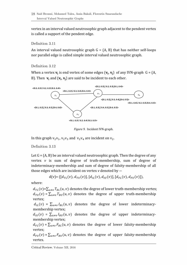
Definition 3.12
When a vertex 𝐯𝐢 is end vertex of some edges (𝐯𝐢, 𝐯𝐣) of any IVN-graph G = (A,
B). Then 𝐯𝐢 and (𝐯𝐢, 𝐯𝐣) are said to be incident to each other.
Figure 9. Incident IVN-graph.
In this graph v2v1, v2v3 and v2v4 are incident on v2.
Definition 3.13
Let G = (A, B) be an interval valued neutrosophic graph. Then the degree of any
vertex v is sum of degree of truth-membership, sum of degree of
indeterminacy-membership and sum of degree of falsity-membership of all
those edges which are incident on vertex v denoted by ―
d(v)= ([𝑑𝑇𝐿(𝑣), 𝑑𝑇𝑈(𝑣)], [𝑑𝐼𝐿(𝑣), 𝑑𝐼𝑈(𝑣)], [𝑑𝐹𝐿(𝑣), 𝑑𝐹𝑈(𝑣)]),
where:
𝑑𝑇𝐿(𝑣)=∑ 𝑇𝐵𝐿(𝑢, 𝑣)𝑢≠𝑣 denotes the degree of lower truth-membership vertex;
𝑑𝑇𝑈(𝑣) = ∑ 𝑇𝐵𝑈(𝑢, 𝑣)𝑢≠𝑣 denotes the degree of upper truth-membership
vertex;
𝑑𝐼𝐿(𝑣) = ∑ 𝐼𝐵𝐿(𝑢, 𝑣)𝑢≠𝑣 denotes the degree of lower indeterminacy-
membership vertex;
𝑑𝐼𝑈(𝑣) = ∑ 𝐼𝐵𝑈(𝑢, 𝑣)𝑢≠𝑣 denotes the degree of upper indeterminacy-
membership vertex;
𝑑𝐹𝐿(𝑣) = ∑ 𝐹𝐵𝐿(𝑢, 𝑣)𝑢≠𝑣 denotes the degree of lower falsity-membership
vertex;
𝑑𝐹𝑈(𝑣) = ∑ 𝐹𝐵𝑈(𝑢, 𝑣)𝑢≠𝑣 denotes the degree of upper falsity-membership
vertex.
𝑣3
<[0.3, 0.5],[ 0.2, 0.3],[0.3, 0.4]> <[0.2, 0.3],[ 0.2, 0.3],[0.1, 0.4]>
<[0.1, 0.3],[ 0.2, 0.4],[0.3, 0.5]>
<[0.1, 0.2],[ 0.3, 0.4],[0.4, 0.5]>
𝑣1 𝑣2
<[0.1, 0.3],[ 0.4, 0.5],[0.4, 0.5]> <[0.1, 0.2],[ 0.3, 0.5],[0.4, 0.6]>
𝑣4
<[0.1, 0.4],[ 0.2, 0.3],[0.4, 0.5]>
<[0.1, 0.2],[ 0.3, 0.4],[0.4, 0.5]>

19
Critical Review. Volume XII, 2016
Said Broumi, Mohamed Talea, Assia Bakali, Florentin Smarandache .
Interval Valued Neutrosophic Graphs
Example 3.14
Let us consider an interval valued neutrosophic graph G = (A, B) of 𝐺∗ = (V, E)
where V = {v1, v2, v3, v4} and E = {v1v2, v2v3, v3v4 , v4v1}.
Figure 10: Degree of vertex of interval valued neutrosophic graph
We have the degree of each vertex as follows:
𝑑(v1)= ([0.3, 0.6], [0.5, 0.9], [0.5, 0.9]), 𝑑(v2)= ([0.4, 0.6], [0.5, 1.0], [0.4, 0.8]),
𝑑(v3)= ([0.4, 0.6], [0.6, 0.9], [0.4, 0.8]), 𝑑(v4)= ([0.3, 0.6], [0.6, 0.8], [0.5, 0.9]).
Definition 3.15
An interval valued neutrosophic graph G= (A, B) is called constant if degree of
each vertex is k =([𝑘1𝐿 , 𝑘1𝑈], [𝑘2𝐿 , 𝑘2𝑈], [𝑘3𝐿 , 𝑘3𝑈]). That is d(𝑣) =([𝑘1𝐿 , 𝑘1𝑈],
[𝑘2𝐿 , 𝑘2𝑈], [𝑘3𝐿 , 𝑘3𝑈]), for all 𝑣 ∈ V.
Example 3.16
Consider an interval valued neutrosophic graph G such that V = {v1, v2, v3, v4}
and E = {v1v2, v2v3, v3v4 , v4v1}.
Figure 11. Constant IVN-graph.
𝑣4
<[0.2, 0.3],[ 0.2, 0.4],[0.1, 0.2]>
<[0.2, 0.3],[ 0.3, 0.4],[0.2, 0.4]>
𝑣3
<[0.3, 0.6],[ 0.2, 0.3],[0.2, 0.3]>
<[0
.1, 0
.3],
[ 0
.3, 0
.4],
[0.3
, 0.5
]>
<[0.4, 0.6],[ 0.1, 0.2],[0.2, 0.3]> <[0.4, 0.5],[ 0.1, 0.3],[0.1, 0.4]>
𝑣1
<[0.2, 0.3],[ 0.2, 0.5],[0.2, 0.4]>
𝑣2
<[0
.2, 0
.3],
[ 0
.3, 0
.5],
[0.2
, 0.4
]>
𝑣4
<[0.2, 0.3],[ 0.2, 0.4],[0.1, 0.2]>
<[0.2, 0.3],[ 0.2, 0.5],[0.2, 0.4]>
𝑣3
<[0.3, 0.6],[ 0.2, 0.3],[0.2, 0.3]>
<[0
.2, 0
.3],
[ 0
.2, 0
.5],
[0.2
, 0.4
]>
<[0.4, 0.6],[ 0.1, 0.2],[0.2, 0.3]> <[0.4, 0.5],[ 0.1, 0.3],[0.1, 0.4]>
𝑣1
<[0.2, 0.3],[ 0.2, 0.5],[0.2, 0.4]>
𝑣2
<[0
.2, 0
.3],
[ 0
.2, 0
.5],
[0.2
, 0.4
]>

20
Said Broumi, Mohamed Talea, Assia Bakali, Florentin Smarandache
Interval Valued Neutrosophic Graphs
Critical Review. Volume XII, 2016
Clearly, G is constant IVN-graph since the degree of 𝒗𝟏, 𝒗𝟐, 𝒗𝟑 and 𝒗𝟒 is ([0.4,
0.6], [0.4, 1], [0.4, 0.8])
Definition 3.17
An interval valued neutrosophic graph G = (A, B) of 𝐺∗= (V, E) is called strong
interval valued neutrosophic graph if
𝑇𝐵𝐿(𝑣𝑖 , 𝑣𝑗) = min[𝑇𝐴𝐿(𝑣𝑖), 𝑇𝐴𝐿(𝑣𝑗)], 𝑇𝐵𝑈(𝑣𝑖 , 𝑣𝑗) = min[𝑇𝐴𝑈(𝑣𝑖),
𝑇𝐴𝑈(𝑣𝑗)]
𝐼𝐵𝐿(𝑣𝑖 , 𝑣𝑗) = max[𝐼𝐴𝐿(𝑣𝑖), 𝐼𝐴𝐿(𝑣𝑗)], 𝐼𝐵𝑈(𝑣𝑖 , 𝑣𝑗) = max[𝐼𝐴𝑈(𝑣𝑖),
𝐼𝐴𝑈(𝑣𝑗)]
𝐹𝐵𝐿(𝑣𝑖 , 𝑣𝑗) = max[𝐹𝐴𝐿(𝑣𝑖), 𝐹𝐴𝐿(𝑣𝑗)], 𝐹𝐵𝑈(𝑣𝑖 , 𝑣𝑗) = max[𝐹𝐴𝑈(𝑣𝑖),
𝐹𝐴𝑈(𝑣𝑗)], for all (𝑣𝑖 , 𝑣𝑗) ∈ E.
Example 3.18
Consider a graph 𝐺∗ such that V = {𝑣1, 𝑣2, 𝑣3, 𝑣4}, E = {𝑣1𝑣2, 𝑣2𝑣3, 𝑣3𝑣4, 𝑣4𝑣1}.
Let A be an interval valued neutrosophic subset of V and let B an interval
valued neutrosophic subset of E denoted by:
𝑣1 𝑣2 𝑣3 𝑣1𝑣2 𝑣2𝑣3 𝑣3𝑣1
𝑇𝐴𝐿 0.3
0.2
0.1
𝑇𝐵𝐿 0.2
0.1
0.1
𝑇𝐴𝑈 0.5 0.3 0.3 𝑇𝐵𝑈 0.3 0.3 0.3
𝐼𝐴𝐿 0.2 0.2 0.2 𝐼𝐵𝐿 0.2 0.2 0.2
𝐼𝐴𝑈 0.3 0.3 0.4 𝐼𝐵𝑈 0.3 0.4 0.4
𝐹𝐴𝐿 0.3 0.1 0.3 𝐹𝐵𝐿 0.3 0.3 0.3
𝐹𝐴𝑈 0.4 0.4 0.5 𝐹𝐵𝑈 0.4 0.4 0.5
Figure 12. Strong IVN-graph.
𝑣3
<[0.3, 0.5],[ 0.2, 0.3],[0.3, 0.4]> <[0.2, 0.3],[ 0.2, 0.3],[0.1, 0.4]>
<[0.1, 0.3],[ 0.2, 0.4],[0.3, 0.5]>
<[0.2, 0.3],[ 0.2, 0.3],[0.3, 0.4]>
𝑣1 𝑣2
<[0.1, 0.3],[ 0.2, 0.4],[0.3, 0.4]> <[0.1, 0.3],[ 0.2, 0.4],[0.3, 0.5]>

21
Critical Review. Volume XII, 2016
Said Broumi, Mohamed Talea, Assia Bakali, Florentin Smarandache .
Interval Valued Neutrosophic Graphs
By routing computations, it is easy to see that G is a strong interval valued
neutrosophic of 𝐺∗.
Proposition 3.19
An interval valued neutrosophic graph is the generalization of interval valued
fuzzy graph
Proof
Suppose G = (V, E) be an interval valued neutrosophic graph. Then by setting
the indeterminacy-membership and falsity-membership values of vertex set
and edge set equals to zero reduces the interval valued neutrosophic graph to
interval valued fuzzy graph.
Proposition 3.20
An interval valued neutrosophic graph is the generalization of interval valued
intuitionistic fuzzy graph
Proof
Suppose G = (V, E) is an interval valued neutrosophic graph. Then by setting
the indeterminacy-membership values of vertex set and edge set equals to
zero reduces the interval valued neutrosophic graph to interval valued
intuitionistic fuzzy graph.
Proposition 3.21
An interval valued neutrosophic graph is the generalization of intuitionistic
fuzzy graph.
Proof
Suppose G = (V, E) is an interval valued neutrosophic graph. Then by setting
the indeterminacy-membership, upper truth-membership and upper falsity-
membership values of vertex set and edge set equals to zero reduces the
interval valued neutrosophic graph to intuitionistic fuzzy graph.
Proposition 3.22
An interval valued neutrosophic graph is the generalization of single valued
neutrosophic graph.
Proof
Suppose G = (V, E) is an interval valued neutrosophic graph. Then by setting
the upper truth-membership equals lower truth-membership, upper

22
Said Broumi, Mohamed Talea, Assia Bakali, Florentin Smarandache
Interval Valued Neutrosophic Graphs
Critical Review. Volume XII, 2016
indeterminacy-membership equals lower indeterminacy-membership and
upper falsity-membership equals lower falsity-membership values of vertex
set and edge set reduces the interval valued neutrosophic graph to single
valued neutrosophic graph.
Definition 3.23
The complement of an interval valued neutrosophic graph G (A, B) on 𝐺∗ is
an interval valued neutrosophic graph �� on 𝐺∗ where:
1. �� =A
2. 𝑇𝐴𝐿 (𝑣𝑖)= 𝑇𝐴𝐿(𝑣𝑖), 𝑇𝐴𝑈
(𝑣𝑖)= 𝑇𝐴𝑈(𝑣𝑖), 𝐼𝐴𝐿 (𝑣𝑖)= 𝐼𝐴𝐿(𝑣𝑖), 𝐼𝐴𝑈
(𝑣𝑖)=
𝐼𝐴𝑈(𝑣𝑖), 𝐹𝐴𝐿 (𝑣𝑖) = 𝐹𝐴𝐿(𝑣𝑖), 𝐹𝐴𝑈
(𝑣𝑖) = 𝐹𝐴𝑈(𝑣𝑖),
for all 𝑣𝑗 ∈ V.
3. 𝑇𝐵𝐿 (𝑣𝑖 , 𝑣𝑗)= min [𝑇𝐴𝐿(𝑣𝑖), 𝑇𝐴𝐿(𝑣𝑗)] − 𝑇𝐵𝐿(𝑣𝑖, 𝑣𝑗),
𝑇𝐵𝑈 (𝑣𝑖 , 𝑣𝑗)= min [𝑇𝐴𝑈(𝑣𝑖), 𝑇𝐴𝑈(𝑣𝑗)] -𝑇𝐵𝑈(𝑣𝑖 , 𝑣𝑗),
𝐼𝐵𝐿 (𝑣𝑖 , 𝑣𝑗)= max [𝐼𝐴𝐿(𝑣𝑖), 𝐼𝐴𝐿(𝑣𝑗)] −
𝐼𝐵𝐿(𝑣𝑖 , 𝑣𝑗), 𝐼𝐵𝑈 (𝑣𝑖 , 𝑣𝑗)= max [𝐼𝐴𝑈(𝑣𝑖), 𝐼𝐴𝑈(𝑣𝑗)] -𝐼𝐵𝑈(𝑣𝑖 , 𝑣𝑗),
and
𝐹𝐵𝐿 (𝑣𝑖 , 𝑣𝑗)= max [𝐹𝐴𝐿(𝑣𝑖), 𝐹𝐴𝐿(𝑣𝑗)] - 𝐹𝐵𝐿(𝑣𝑖 , 𝑣𝑗),
𝐹𝐵𝑈 (𝑣𝑖 , 𝑣𝑗)= max [𝐹𝐴𝑈(𝑣𝑖), 𝐹𝐴𝑈(𝑣𝑗)] - 𝐹𝐵𝑈(𝑣𝑖 , 𝑣𝑗),
for all (𝑣𝑖 , 𝑣𝑗) ∈ E
Remark 3.24
If G = (V, E) is an interval valued neutrosophic graph on 𝐺∗. Then from above
definition, it follow that �� is given by the interval valued neutrosophic graph
G = (V , E ) on G∗ where V =V and ―
TBL (vi, vj)= min [TAL(vi), TA(vj)]-TBL(vi, vj),
TBU (vi, vj)= min [TAU(vi), TA(vj)]-TBU(vi, vj),
IBL (vi, vj)= max [IAL(vi), IAL(vj)]-IBL(vi, vj),
IBU (vi, vj)= max [IAU(vi), IAU(vj)]-IBU(vi, vj),
and
FBL (vi, vj) = max [FAL(vi), FAL(vj)]-FBL(vi, vj), FBU
(vi, vj)
= max [FAU(vi), FAU(vj)]-FBU(vi, vj), For all (vi, vj) ∈ E.
23
Critical Review. Volume XII, 2016
Said Broumi, Mohamed Talea, Assia Bakali, Florentin Smarandache .
Interval Valued Neutrosophic Graphs
Thus 𝑇𝐵𝐿 =𝑇𝐵𝐿 , 𝑇𝐵𝑈
=𝑇𝐵𝑈𝐿 , 𝐼𝐵𝐿 =𝐼𝐵𝐿 , 𝐼𝐵𝑈
=𝐼𝐵𝑈 , and 𝐹𝐵𝐿 =𝐹𝐵𝐿 , 𝐹𝐵𝑈
=𝐹𝐵𝑈 on V,
where E =( [𝑇𝐵𝐿, 𝑇𝐵𝑈], [𝐼𝐵𝐿 , 𝐼𝐵𝑈], [𝐹𝐵𝐿 , 𝐹𝐵𝑈]) is the interval valued neutrosophic
relation on V. For any interval valued neutrosophic graph G, �� is strong
interval valued neutrosophic graph and G ⊆ ��.
Proposition 3.25
G= �� if and only if G is a strong interval valued neutrosophic graph.
Proof
It is obvious.
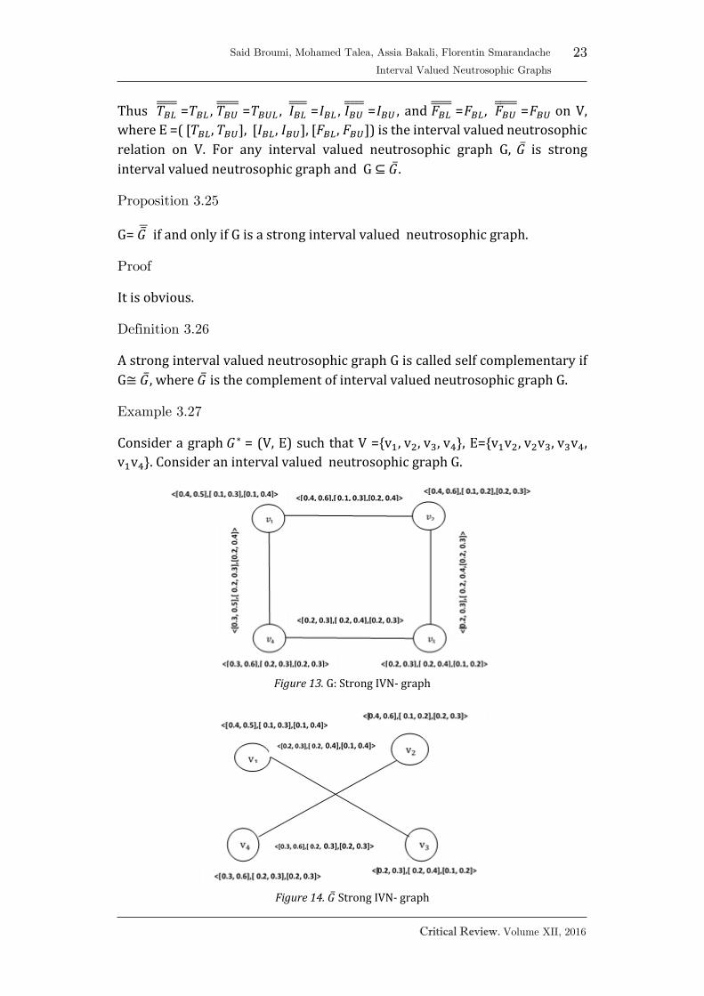
Definition 3.26
A strong interval valued neutrosophic graph G is called self complementary if
G≅ ��, where �� is the complement of interval valued neutrosophic graph G.
Example 3.27
Consider a graph 𝐺∗ = (V, E) such that V ={v1, v2, v3, v4}, E={v1v2, v2v3, v3v4,
v1v4}. Consider an interval valued neutrosophic graph G.
Figure 13. G: Strong IVN- graph
Figure 14. �� Strong IVN- graph

24
Said Broumi, Mohamed Talea, Assia Bakali, Florentin Smarandache
Interval Valued Neutrosophic Graphs
Critical Review. Volume XII, 2016
Figure 15. �� Strong IVN- graph
Clearly, G≅ �� , hence G is self complementary.
Proposition 3.26
Let G=(A, B) be a strong interval valued neutrosophic graph. If ―
𝑇𝐵𝐿(𝑣𝑖 , 𝑣𝑗) = min [𝑇𝐴𝐿(𝑣𝑖), 𝑇𝐴𝐿(𝑣𝑗)]
𝑇𝐵𝑈(𝑣𝑖, 𝑣𝑗) = min [𝑇𝐴𝑈(𝑣𝑖), 𝑇𝐴𝑈(𝑣𝑗)]
𝐼𝐵𝐿(𝑣𝑖 , 𝑣𝑗) = max [𝐼𝐴𝐿(𝑣𝑖), 𝐼𝐴𝐿(𝑣𝑗)]
𝐼𝐵𝑈(𝑣𝑖 , 𝑣𝑗) = max [𝐼𝐴𝑈(𝑣𝑖), 𝐼𝐴𝑈(𝑣𝑗)]
𝐹𝐵𝐿(𝑣𝑖 , 𝑣𝑗) = max [𝐹𝐴𝐿(𝑣𝑖), 𝐹𝐴𝐿(𝑣𝑗)]
𝐹𝐵𝑈(𝑣𝑖 , 𝑣𝑗) = max [𝐹𝐴𝑈(𝑣𝑖), 𝐹𝐴𝑈(𝑣𝑗)]
for all 𝑣𝑖 , 𝑣𝑗 ∈ V, then G is self complementary.
Proof
Let G = (A, B) be a strong interval valued neutrosophic graph such that ―
𝑇𝐵𝐿(𝑣𝑖 , 𝑣𝑗) = min [𝑇𝐴𝐿(𝑣𝑖), 𝑇𝐴𝐿(𝑣𝑗)];
𝑇𝐵𝑈(𝑣𝑖, 𝑣𝑗) = min [𝑇𝐴𝑈(𝑣𝑖), 𝑇𝐴𝑈(𝑣𝑗)];
𝐼𝐵𝐿(𝑣𝑖 , 𝑣𝑗) = max [𝐼𝐴𝐿(𝑣𝑖), 𝐼𝐴𝐿(𝑣𝑗)];
𝐼𝐵𝑈(𝑣𝑖 , 𝑣𝑗) = max [𝐼𝐴𝑈(𝑣𝑖), 𝐼𝐴𝑈(𝑣𝑗)];
𝐹𝐵𝐿(𝑣𝑖 , 𝑣𝑗) = max [𝐹𝐴𝐿(𝑣𝑖), 𝐹𝐴𝐿(𝑣𝑗)];
𝐹𝐵𝑈(𝑣𝑖 , 𝑣𝑗) = max [𝐹𝐴𝑈(𝑣𝑖), 𝐹𝐴𝑈(𝑣𝑗)],
for all 𝑣𝑖 , 𝑣𝑗 ∈ V, then G≈ �� under the identity map I: V →V, hence G is self
complementary.
𝑣4
<[0.2, 0.3],[ 0.2, 0.4],[0.1, 0.2]>
<[0.2, 0.3],[ 0.2, 0.4],[0.2, 0.3]>
𝑣3
<[0.3, 0.6],[ 0.2, 0.3],[0.2, 0.3]>
<[0
.3, 0
.5],
[ 0
.2, 0
.3],
[0.2
, 0.4
]>
<[0.4, 0.6],[ 0.1, 0.2],[0.2, 0.3]> <[0.4, 0.5],[ 0.1, 0.3],[0.1, 0.4]>
𝑣1
<[0.4, 0.6],[ 0.1, 0.3],[0.2, 0.4]>
𝑣2
<[0
.2, 0
.3],
[ 0
.2, 0
.4,[
0.2
, 0.3
]>

25
Critical Review. Volume XII, 2016
Said Broumi, Mohamed Talea, Assia Bakali, Florentin Smarandache .
Interval Valued Neutrosophic Graphs
Proposition 3.27
Let G be a self complementary interval valued neutrosophic graph. Then ―
∑ 𝑇𝐵𝐿(𝑣𝑖 , 𝑣𝑗)𝑣𝑖≠𝑣𝑗 =
1
2 ∑ min [𝑇𝐴𝐿(𝑣𝑖), 𝑇𝐴𝐿(𝑣𝑗)]𝑣𝑖≠𝑣𝑗
∑ 𝑇𝐵𝑈(𝑣𝑖, 𝑣𝑗)𝑣𝑖≠𝑣𝑗 =
1
2 ∑ min [𝑇𝐴𝑈(𝑣𝑖), 𝑇𝐴𝑈(𝑣𝑗)]𝑣𝑖≠𝑣𝑗
∑ 𝐼𝐵𝐿(𝑣𝑖 , 𝑣𝑗)𝑣𝑖≠𝑣𝑗 =
1
2 ∑ max [𝐼𝐴𝐿(𝑣𝑖), 𝐼𝐴𝐿(𝑣𝑗)]𝑣𝑖≠𝑣𝑗
∑ 𝐼𝐵𝑈(𝑣𝑖 , 𝑣𝑗)𝑣𝑖≠𝑣𝑗 =
1
2 ∑ max [𝐼𝐴𝑈(𝑣𝑖), 𝐼𝐴𝑈(𝑣𝑗)]𝑣𝑖≠𝑣𝑗
∑ 𝐹𝐵𝐿(𝑣𝑖 , 𝑣𝑗)𝑣𝑖≠𝑣𝑗 =
1
2∑ max [𝐹𝐴𝐿(𝑣𝑖), 𝐹𝐴𝐿(𝑣𝑗)]𝑣𝑖≠𝑣𝑗
∑ 𝐹𝐵𝑈(𝑣𝑖 , 𝑣𝑗)𝑣𝑖≠𝑣𝑗 =
1
2∑ max [𝐹𝐴𝑈(𝑣𝑖), 𝐹𝐴𝑈(𝑣𝑗)]𝑣𝑖≠𝑣𝑗
.
Proof
If G be a self complementary interval valued neutrosophic graph. Then there
exist an isomorphism f: 𝑉1 → 𝑉1 satisfying
𝑇𝑉1 (𝑓(𝑣𝑖)) = 𝑇𝑉1
(𝑓(𝑣𝑖)) = 𝑇𝑉1(𝑣𝑖)
𝐼𝑉1 (𝑓(𝑣𝑖)) = 𝐼𝑉1
(𝑓(𝑣𝑖)) = 𝐼𝑉1(𝑣𝑖)
𝐹𝑉1 (𝑓(𝑣𝑖)) = 𝐹𝑉1
(𝑓(𝑣𝑖)) = 𝐹𝑉1(𝑣𝑖)
for all 𝑣𝑖 ∈ 𝑉1, and ―
𝑇𝐸1 (𝑓(𝑣𝑖), 𝑓(𝑣𝑗)) =𝑇𝐸1
(𝑓(𝑣𝑖), 𝑓(𝑣𝑗)) =𝑇𝐸1(𝑣𝑖 , 𝑣𝑗)
𝐼𝐸1 (𝑓(𝑣𝑖), 𝑓(𝑣𝑗)) =𝐼𝐸1
(𝑓(𝑣𝑖), 𝑓(𝑣𝑗)) =𝐼𝐸1(𝑣𝑖 , 𝑣𝑗)
𝐹𝐸1 (𝑓(𝑣𝑖), 𝑓(𝑣𝑗)) =𝐹𝐸1
(𝑓(𝑣𝑖), 𝑓(𝑣𝑗)) =𝐹𝐸1(𝑣𝑖 , 𝑣𝑗)
for all (𝑣𝑖 , 𝑣𝑗) ∈ 𝐸1.
We have
𝑇𝐸1 (𝑓(𝑣𝑖), 𝑓(𝑣𝑗)) = min [𝑇𝑉1
(𝑓(𝑣𝑖)), 𝑇𝑉1 (𝑓(𝑣𝑗))] − 𝑇𝐸1
(𝑓(𝑣𝑖), 𝑓(𝑣𝑗))
i.e, 𝑇𝐸1(𝑣𝑖 , 𝑣𝑗) = min [𝑇𝑉1
(𝑣𝑖), 𝑇𝑉1(𝑣𝑗)] − 𝑇𝐸1
(𝑓(𝑣𝑖), 𝑓(𝑣𝑗))
𝑇𝐸1(𝑣𝑖 , 𝑣𝑗) = min [𝑇𝑉1
(𝑣𝑖), 𝑇𝑉1(𝑣𝑗)] − 𝑇𝐸1
(𝑣𝑖 , 𝑣𝑗).
That is ―
∑ 𝑇𝐸1(𝑣𝑖, 𝑣𝑗)𝑣𝑖≠𝑣𝑗
+∑ 𝑇𝐸1(𝑣𝑖, 𝑣𝑗)𝑣𝑖≠𝑣𝑗
= ∑ min [𝑇𝑉1(𝑣𝑖), 𝑇𝑉1
(𝑣𝑗)]𝑣𝑖≠𝑣𝑗
∑ 𝐼𝐸1(𝑣𝑖 , 𝑣𝑗)𝑣𝑖≠𝑣𝑗
+∑ 𝐼𝐸1(𝑣𝑖 , 𝑣𝑗)𝑣𝑖≠𝑣𝑗
= ∑ max [𝐼𝑉1(𝑣𝑖), 𝐼𝑉1
(𝑣𝑗)]𝑣𝑖≠𝑣𝑗
∑ 𝐹𝐸1(𝑣𝑖 , 𝑣𝑗)𝑣𝑖≠𝑣𝑗
+∑ 𝐹𝐸1(𝑣𝑖 , 𝑣𝑗)𝑣𝑖≠𝑣𝑗
= ∑ max [𝐹𝑉1(𝑣𝑖), 𝐹𝑉1
(𝑣𝑗)]𝑣𝑖≠𝑣𝑗

26
Said Broumi, Mohamed Talea, Assia Bakali, Florentin Smarandache
Interval Valued Neutrosophic Graphs
Critical Review. Volume XII, 2016
2 ∑ 𝑇𝐸1(𝑣𝑖, 𝑣𝑗)𝑣𝑖≠𝑣𝑗
= ∑ min [𝑇𝑉1(𝑣𝑖), 𝑇𝑉1
(𝑣𝑗)]𝑣𝑖≠𝑣𝑗
2 ∑ 𝐼𝐸1(𝑣𝑖 , 𝑣𝑗)𝑣𝑖≠𝑣𝑗
= ∑ max [𝐼𝑉1(𝑣𝑖), 𝐼𝑉1
(𝑣𝑗)]𝑣𝑖≠𝑣𝑗
2∑ 𝐹𝐸1(𝑣𝑖 , 𝑣𝑗)𝑣𝑖≠𝑣𝑗
= ∑ max [𝐹𝑉1(𝑣𝑖), 𝐹𝑉1
(𝑣𝑗)]𝑣𝑖≠𝑣𝑗.
From these equations, Proposition 3.27 holds.
Proposition 3.28
Let 𝐺1 and 𝐺2 be strong interval valued neutrosophic graph, 𝐺1 ≈ 𝐺2
(isomorphism).
Proof
Assume that 𝐺1 and 𝐺2 are isomorphic, there exists a bijective map f: 𝑉1 → 𝑉2
satisfying
𝑇𝑉1(𝑣𝑖) =𝑇𝑉2
(𝑓(𝑣𝑖)),
𝐼𝑉1(𝑣𝑖) =𝐼𝑉2
(𝑓(𝑣𝑖)),
𝐹𝑉1(𝑣𝑖) =𝐹𝑉2
(𝑓(𝑣𝑖)),
for all 𝑣𝑖 ∈ 𝑉1, and
𝑇𝐸1(𝑣𝑖 , 𝑣𝑗) =𝑇𝐸2
(𝑓(𝑣𝑖), 𝑓(𝑣𝑗)),
𝐼𝐸1(𝑣𝑖 , 𝑣𝑗) =𝐼𝐸2
(𝑓(𝑣𝑖), 𝑓(𝑣𝑗)),
𝐹𝐸1(𝑣𝑖 , 𝑣𝑗) = 𝐹𝐸2
(𝑓(𝑣𝑖), 𝑓(𝑣𝑗)),
for all (𝑣𝑖 , 𝑣𝑗) ∈ 𝐸1.
By Definition 3.21, we have
𝑇𝐸1 (𝑣𝑖 , 𝑣𝑗)= min [𝑇𝑉1
(𝑣𝑖), 𝑇𝑉1(𝑣𝑗)] −𝑇𝐸1
(𝑣𝑖 , 𝑣𝑗)
= min [𝑇𝑉2(𝑓(𝑣𝑖)), 𝑇𝑉2
(𝑓(𝑣𝑗))] −𝑇𝐸2(𝑓(𝑣𝑖), 𝑓(𝑣𝑗)),
= 𝑇𝐸2 (𝑓(𝑣𝑖), 𝑓(𝑣𝑗)),
𝐼𝐸1 (𝑣𝑖 , 𝑣𝑗)= max [𝐼𝑉1
(𝑣𝑖), 𝐼𝑉1(𝑣𝑗)] −𝐼𝐸1
(𝑣𝑖 , 𝑣𝑗)
= max[𝐼𝑉2(𝑓(𝑣𝑖)), 𝐼𝑉2
(𝑓(𝑣𝑗))] −𝐼𝐸2(𝑓(𝑣𝑖), 𝑓(𝑣𝑗)),
= 𝐼𝐸2 (𝑓(𝑣𝑖), 𝑓(𝑣𝑗)),
𝐹𝐸1 (𝑣𝑖 , 𝑣𝑗)= min [𝐹𝑉1
(𝑣𝑖), 𝐹𝑉1(𝑣𝑗)] −𝐹𝐸1
(𝑣𝑖 , 𝑣𝑗)
= min [𝐹𝑉2(𝑓(𝑣𝑖)), 𝐹𝑉2
(𝑓(𝑣𝑗))] −𝐹𝐸2(𝑓(𝑣𝑖), 𝑓(𝑣𝑗)),
= 𝐹𝐸2 (𝑓(𝑣𝑖), 𝑓(𝑣𝑗)),
for all (𝑣𝑖 , 𝑣𝑗) ∈ 𝐸1, hence 𝐺1 ≈ 𝐺2
. The converse is straightforward.
27
Critical Review. Volume XII, 2016
Said Broumi, Mohamed Talea, Assia Bakali, Florentin Smarandache .
Interval Valued Neutrosophic Graphs
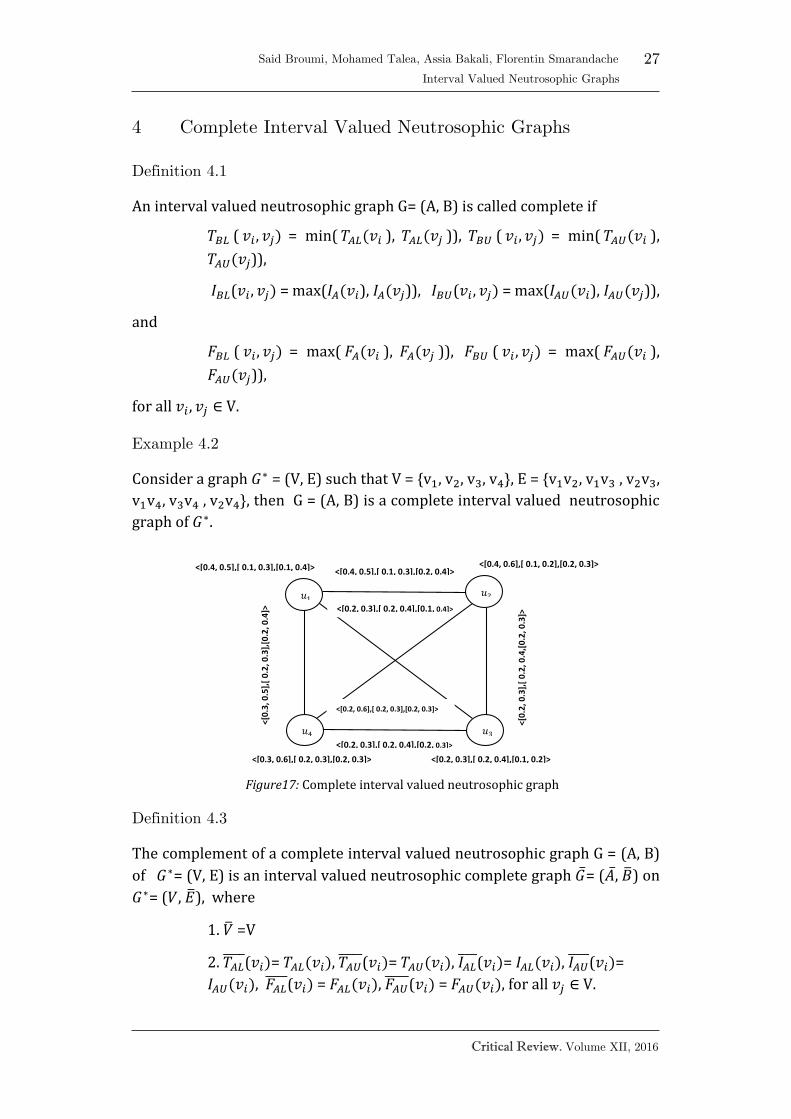
4 Complete Interval Valued Neutrosophic Graphs
Definition 4.1
An interval valued neutrosophic graph G= (A, B) is called complete if
𝑇𝐵𝐿 ( 𝑣𝑖 , 𝑣𝑗) = min( 𝑇𝐴𝐿(𝑣𝑖 ), 𝑇𝐴𝐿(𝑣𝑗 )), 𝑇𝐵𝑈 ( 𝑣𝑖 , 𝑣𝑗) = min( 𝑇𝐴𝑈(𝑣𝑖 ),
𝑇𝐴𝑈(𝑣𝑗)),
𝐼𝐵𝐿(𝑣𝑖 , 𝑣𝑗) = max(𝐼𝐴(𝑣𝑖), 𝐼𝐴(𝑣𝑗)), 𝐼𝐵𝑈(𝑣𝑖 , 𝑣𝑗) = max(𝐼𝐴𝑈(𝑣𝑖), 𝐼𝐴𝑈(𝑣𝑗)),
and
𝐹𝐵𝐿 ( 𝑣𝑖 , 𝑣𝑗) = max( 𝐹𝐴(𝑣𝑖 ), 𝐹𝐴(𝑣𝑗 )), 𝐹𝐵𝑈 ( 𝑣𝑖 , 𝑣𝑗) = max( 𝐹𝐴𝑈(𝑣𝑖 ),
𝐹𝐴𝑈(𝑣𝑗)),
for all 𝑣𝑖 , 𝑣𝑗 ∈ V.
Example 4.2
Consider a graph 𝐺∗ = (V, E) such that V = {v1, v2, v3, v4}, E = {v1v2, v1v3 , v2v3,
v1v4, v3v4 , v2v4}, then G = (A, B) is a complete interval valued neutrosophic
graph of 𝐺∗.
Figure17: Complete interval valued neutrosophic graph
Definition 4.3
The complement of a complete interval valued neutrosophic graph G = (A, B)
of 𝐺∗= (V, E) is an interval valued neutrosophic complete graph ��= (��, ��) on
𝐺∗= (𝑉, ��), where
1. �� =V
2. 𝑇𝐴𝐿 (𝑣𝑖)= 𝑇𝐴𝐿(𝑣𝑖), 𝑇𝐴𝑈
(𝑣𝑖)= 𝑇𝐴𝑈(𝑣𝑖), 𝐼𝐴𝐿 (𝑣𝑖)= 𝐼𝐴𝐿(𝑣𝑖), 𝐼𝐴𝑈
(𝑣𝑖)=
𝐼𝐴𝑈(𝑣𝑖), 𝐹𝐴𝐿 (𝑣𝑖) = 𝐹𝐴𝐿(𝑣𝑖), 𝐹𝐴𝑈
(𝑣𝑖) = 𝐹𝐴𝑈(𝑣𝑖), for all 𝑣𝑗 ∈ V.
<[0.2, 0.3],[ 0.2, 0.4],[0.1, 0.4]>
𝑢4
<[0.2, 0.3],[ 0.2, 0.4],[0.1, 0.2]>
<[0.2, 0.6],[ 0.2, 0.3],[0.2, 0.3]>
𝑢3
<[0.3, 0.6],[ 0.2, 0.3],[0.2, 0.3]>
<[0
.3, 0
.5],
[ 0
.2, 0
.3],
[0.2
, 0.4
]>
<[0.4, 0.6],[ 0.1, 0.2],[0.2, 0.3]> <[0.4, 0.5],[ 0.1, 0.3],[0.1, 0.4]>
𝑢1
<[0.4, 0.5],[ 0.1, 0.3],[0.2, 0.4]>
𝑢2
<[0
.2, 0
.3],
[ 0
.2, 0
.4,[
0.2
, 0.3
]>
<[0.2, 0.3],[ 0.2, 0.4],[0.2, 0.3]>
28
Said Broumi, Mohamed Talea, Assia Bakali, Florentin Smarandache
Interval Valued Neutrosophic Graphs
Critical Review. Volume XII, 2016
3. 𝑇𝐵𝐿 (𝑣𝑖 , 𝑣𝑗)= min [𝑇𝐴𝐿(𝑣𝑖), 𝑇𝐴𝐿(𝑣𝑗)] − 𝑇𝐵𝐿(𝑣𝑖, 𝑣𝑗),
𝑇𝐵𝑈 (𝑣𝑖 , 𝑣𝑗)= min [𝑇𝐴𝑈(𝑣𝑖), 𝑇𝐴𝑈(𝑣𝑗)] − 𝑇𝐵𝑈(𝑣𝑖 , 𝑣𝑗),
𝐼𝐵𝐿 (𝑣𝑖 , 𝑣𝑗)= max [𝐼𝐴𝐿(𝑣𝑖), 𝐼𝐴𝐿(𝑣𝑗)] − 𝐼𝐵𝐿(𝑣𝑖 , 𝑣𝑗),
𝐼𝐵𝑈 (𝑣𝑖 , 𝑣𝑗)= max [𝐼𝐴𝑈(𝑣𝑖), 𝐼𝐴𝑈(𝑣𝑗)] − 𝐼𝐵𝑈(𝑣𝑖, 𝑣𝑗),
and
𝐹𝐵𝐿 (𝑣𝑖 , 𝑣𝑗)= max [𝐹𝐴𝐿(𝑣𝑖), 𝐹𝐴𝐿(𝑣𝑗)] − 𝐹𝐵𝐿(𝑣𝑖 , 𝑣𝑗),
𝐹𝐵𝑈 (𝑣𝑖 , 𝑣𝑗)= max [𝐹𝐴𝑈(𝑣𝑖), 𝐹𝐴𝑈(𝑣𝑗)] − 𝐹𝐵𝑈(𝑣𝑖 , 𝑣𝑗),
for all (𝑣𝑖 , 𝑣𝑗) ∈ E.
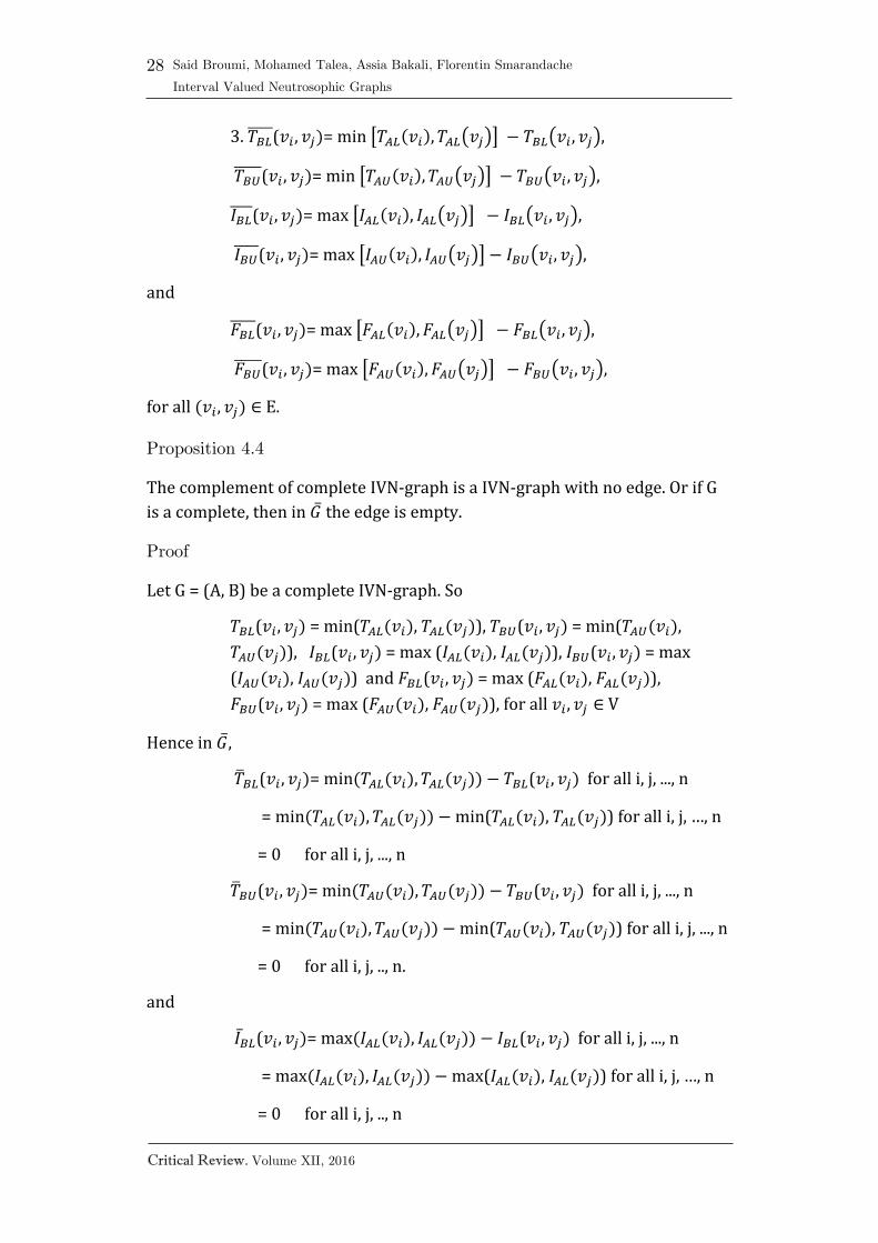
Proposition 4.4
The complement of complete IVN-graph is a IVN-graph with no edge. Or if G
is a complete, then in �� the edge is empty.
Proof
Let G = (A, B) be a complete IVN-graph. So
𝑇𝐵𝐿(𝑣𝑖 , 𝑣𝑗) = min(𝑇𝐴𝐿(𝑣𝑖), 𝑇𝐴𝐿(𝑣𝑗)), 𝑇𝐵𝑈(𝑣𝑖 , 𝑣𝑗) = min(𝑇𝐴𝑈(𝑣𝑖),
𝑇𝐴𝑈(𝑣𝑗)), 𝐼𝐵𝐿(𝑣𝑖 , 𝑣𝑗) = max (𝐼𝐴𝐿(𝑣𝑖), 𝐼𝐴𝐿(𝑣𝑗)), 𝐼𝐵𝑈(𝑣𝑖 , 𝑣𝑗) = max
(𝐼𝐴𝑈(𝑣𝑖), 𝐼𝐴𝑈(𝑣𝑗)) and 𝐹𝐵𝐿(𝑣𝑖 , 𝑣𝑗) = max (𝐹𝐴𝐿(𝑣𝑖), 𝐹𝐴𝐿(𝑣𝑗)),
𝐹𝐵𝑈(𝑣𝑖 , 𝑣𝑗) = max (𝐹𝐴𝑈(𝑣𝑖), 𝐹𝐴𝑈(𝑣𝑗)), for all 𝑣𝑖 , 𝑣𝑗 ∈ V
Hence in ��,
��𝐵𝐿(𝑣𝑖 , 𝑣𝑗)= min(𝑇𝐴𝐿(𝑣𝑖), 𝑇𝐴𝐿(𝑣𝑗)) − 𝑇𝐵𝐿(𝑣𝑖 , 𝑣𝑗) for all i, j, ..., n
= min(𝑇𝐴𝐿(𝑣𝑖), 𝑇𝐴𝐿(𝑣𝑗)) − min(𝑇𝐴𝐿(𝑣𝑖), 𝑇𝐴𝐿(𝑣𝑗)) for all i, j, …, n
= 0 for all i, j, ..., n
��𝐵𝑈(𝑣𝑖 , 𝑣𝑗)= min(𝑇𝐴𝑈(𝑣𝑖), 𝑇𝐴𝑈(𝑣𝑗)) − 𝑇𝐵𝑈(𝑣𝑖 , 𝑣𝑗) for all i, j, ..., n
= min(𝑇𝐴𝑈(𝑣𝑖), 𝑇𝐴𝑈(𝑣𝑗)) − min(𝑇𝐴𝑈(𝑣𝑖), 𝑇𝐴𝑈(𝑣𝑗)) for all i, j, ..., n
= 0 for all i, j, .., n.
and
𝐼��𝐿(𝑣𝑖 , 𝑣𝑗)= max(𝐼𝐴𝐿(𝑣𝑖), 𝐼𝐴𝐿(𝑣𝑗)) − 𝐼𝐵𝐿(𝑣𝑖 , 𝑣𝑗) for all i, j, ..., n
= max(𝐼𝐴𝐿(𝑣𝑖), 𝐼𝐴𝐿(𝑣𝑗)) − max(𝐼𝐴𝐿(𝑣𝑖), 𝐼𝐴𝐿(𝑣𝑗)) for all i, j, …, n
= 0 for all i, j, .., n
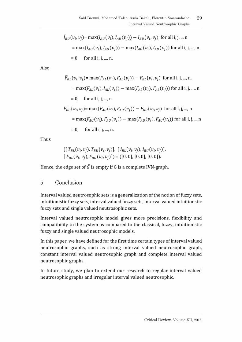
29
Critical Review. Volume XII, 2016
Said Broumi, Mohamed Talea, Assia Bakali, Florentin Smarandache .
Interval Valued Neutrosophic Graphs
𝐼��𝑈(𝑣𝑖 , 𝑣𝑗)= max(𝐼𝐴𝑈(𝑣𝑖), 𝐼𝐴𝑈(𝑣𝑗)) − 𝐼𝐵𝑈(𝑣𝑖 , 𝑣𝑗) for all i, j, .., n
= max(𝐼𝐴𝑈(𝑣𝑖), 𝐼𝐴𝑈(𝑣𝑗)) − max(𝐼𝐴𝑈(𝑣𝑖), 𝐼𝐴𝑈(𝑣𝑗)) for all i, j, …, n
= 0 for all i, j, ..., n.
Also
��𝐵𝐿(𝑣𝑖 , 𝑣𝑗)= max(𝐹𝐴𝐿(𝑣𝑖), 𝐹𝐴𝐿(𝑣𝑗)) − 𝐹𝐵𝐿(𝑣𝑖 , 𝑣𝑗) for all i, j, ..., n.
= max(𝐹𝐴𝐿(𝑣𝑖), 𝐼𝐴𝐿(𝑣𝑗)) − max(𝐹𝐴𝐿(𝑣𝑖), 𝐹𝐴𝐿(𝑣𝑗)) for all i, j, …, n
= 0, for all i, j, ..., n.
��𝐵𝑈(𝑣𝑖 , 𝑣𝑗)= max(𝐹𝐴𝑈(𝑣𝑖), 𝐹𝐴𝑈(𝑣𝑗)) − 𝐹𝐵𝑈(𝑣𝑖 , 𝑣𝑗) for all i, j, ..., n
= max(𝐹𝐴𝑈(𝑣𝑖), 𝐹𝐴𝑈(𝑣𝑗)) − max(𝐹𝐴𝑈(𝑣𝑖), 𝐹𝐴𝑈(𝑣𝑗)) for all i, j, ...,n
= 0, for all i, j, ..., n.
Thus
([ ��𝐵𝐿(𝑣𝑖 , 𝑣𝑗), ��𝐵𝑈(𝑣𝑖 , 𝑣𝑗)], [ 𝐼��𝐿(𝑣𝑖 , 𝑣𝑗), 𝐼��𝑈(𝑣𝑖 , 𝑣𝑗)],
[ ��𝐵𝐿(𝑣𝑖 , 𝑣𝑗), ��𝐵𝑈(𝑣𝑖 , 𝑣𝑗)]) = ([0, 0], [0, 0], [0, 0]).
Hence, the edge set of �� is empty if G is a complete IVN-graph.
5 Conclusion
Interval valued neutrosophic sets is a generalization of the notion of fuzzy sets,
intuitionistic fuzzy sets, interval valued fuzzy sets, interval valued intuitionstic
fuzzy sets and single valued neutrosophic sets.
Interval valued neutrosophic model gives more precisions, flexibility and
compatibility to the system as compared to the classical, fuzzy, intuitionistic
fuzzy and single valued neutrosophic models.
In this paper, we have defined for the first time certain types of interval valued
neutrosophic graphs, such as strong interval valued neutrosophic graph,
constant interval valued neutrosophic graph and complete interval valued
neutrosophic graphs.
In future study, we plan to extend our research to regular interval valued
neutrosophic graphs and irregular interval valued neutrosophic.

30
Said Broumi, Mohamed Talea, Assia Bakali, Florentin Smarandache
Interval Valued Neutrosophic Graphs
Critical Review. Volume XII, 2016
References
[1] V. Devadoss, A. Rajkumar & N. J. P. Praveena. A Study on Miracles
through Holy Bible using Neutrosophic Cognitive Maps (NCMS) , in
“International Journal of Computer Applications”, 69(3), 2013.
[2] Mohamed Ismayil and A. Mohamed Ali. On Strong Interval-Valued
Intuitionistic Fuzzy Graph, in “International Journal of Fuzzy
Mathematics and Systems”, Volume 4, Number 2, 2014, pp. 161-168.
[3] Q. Ansari, R. Biswas & S. Aggarwal. Neutrosophic classifier: An
extension of fuzzy classifier, in “Applied Soft Computing”, 13, 2013,
pp. 563-573, http://dx.doi.org/10.1016/j.asoc.2012.08.002.
[4] Aydoğdu, On Similarity and Entropy of Single Valued Neutro-sophic
Sets, in “Gen. Math. Notes”, Vol. 29, No. 1, 2015, pp. 67-74.
[5] Q. Ansari, R. Biswas & S. Aggarwal. Neutrosophication of Fuzzy
Models, poster presentation at IEEE Workshop On Computational
Intelligence: Theories, Applications and Future Directions (hosted
by IIT Kanpur), 14th July 2013.
[6] Q. Ansari, R. Biswas & S. Aggarwal. Extension to fuzzy logic
representation: Moving towards neutrosophic logic - A new
laboratory rat, at the Fuzzy Systems IEEE International Conference,
2013, 1–8, doi:10.1109/FUZZ-IEEE.2013.6622412.
[7] Nagoor Gani and M. Basheer Ahamed. Order and Size in Fuzzy Graphs, in
“Bulletin of Pure and Applied Sciences”, Vol 22E, No. 1, 2003, pp. 145-
148.
[8] Nagoor Gani, A. and S. Shajitha Begum. Degree, Order and Size in
Intuitionistic Fuzzy Graphs, in “International Journal of Algorithms,
Computing and Mathematics”, (3)3, 2010.
[9] Nagoor Gani and S. R. Latha. On Irregular Fuzzy Graphs, in “Applied
Mathematical Sciences”, Vol. 6, no. 11, 2012, pp. 517-523.
[10] F. Smarandache. Refined Literal Indeterminacy and the Multiplication
Law of Sub-Indeterminacies, in “Neutrosophic Sets and Systems”, Vol. 9,
2015, pp. 58- 63.
[11] F. Smarandache. Types of Neutrosophic Graphs and Neutrosophic
Algebraic Structures together with their Applications in Technology,
seminar, Universitatea Transilvania din Brasov, Facultatea de Design de
Produs si Mediu, Brasov, Romania, 6 June 2015.
[12] F. Smarandache, Symbolic Neutrosophic Theory, Europanova asbl,
Brussels, 2015, 195p.
[13] F. Smarandache. Neutrosophic set - a generalization of the intuitionistic
fuzzy set, Granular Computing, 2006 IEEE International Conference,
(2006)38 – 42, DOI: 10.1109/GRC.2006.1635754.

31
Critical Review. Volume XII, 2016
Said Broumi, Mohamed Talea, Assia Bakali, Florentin Smarandache .
Interval Valued Neutrosophic Graphs
[14] F. Smarandache. A geometric interpretation of the neutrosophic set — A
generalization of the intuitionistic fuzzy set, Granular Computing (GrC),
2011 IEEE International Conference, 2011, pp. 602 – 606, DOI
10.1109/GRC.2011.6122665.
[15] Gaurav Garg, Kanika Bhutani, Megha Kumar and Swati Aggarwal. Hybrid
model for medical diagnosis using Neutrosophic Cognitive Maps with
Genetic Algorithms, FUZZ-IEEE 2015 (IEEE International conference
on fuzzy systems).
[16] H. Wang,. Y. Zhang, R. Sunderraman. Truth-value based interval
neutrosophic sets, Granular Computing, 2005 IEEE International
Conference, Vol. 1, 2005, pp. 274 - 277
DOI: 10.1109/GRC.2005.1547284.
[17] H. Wang, F. Smarandache, Y. Zhang, and R. Sunderraman, Single
valued Neutrosophic Sets, Multisspace and Multistructure 4, 2010, pp.
410-413.
[18] H. Wang, F. Smarandache, Y.Q. Zhang and R. Sunderram. An Interval
neutrosophic sets and logic: theory and applications in computing. Hexis,
Arizona, 2005.
[19] H. Y. Zhang , J. Q. Wang , X. H. Chen. Interval neutrosophic sets and
their application in multicriteria decision making problems, The
Scientific World Journal, (2014), DOI:10.1155/2014/ 645953.
[20] H, Zhang, J .Wang, X. Chen. An outranking approach for multi-criteria
decision-making problems with interval valued neutrosophic sets, Neural
Computing and Applications, 2015, pp. 1-13.
[21] H.Y. Zhang, P. Ji, J.Q. Wang & X. H. Chen. An Improved Weighted
Correlation Coefficient Based on Integrated Weight for Interval
Neutrosophic Sets and its Application in Multi-criteria Decision-making
Problems, International Journal of Computational Intelligence Systems,
V8, Issue 6 (2015), DOI:10.1080/18756891.2015.1099917.
[22] Deli, M. Ali, F. Smarandache. Bipolar neutrosophic sets and their
application based on multi-criteria decision making problems,
Advanced Mechatronic Systems (ICAMechS), International
Conference, 2015, pp. 249 – 254.
[23] Turksen. Interval valued fuzzy sets based on normal forms, Fuzzy Sets
and Systems, vol. 20, 1986, pp. 191-210 .
[24] J. Ye. vector similarity measures of simplified neutrosophic sets and their
application in multicriteria decision making, International Journal of
Fuzzy Systems, Vol. 16, No. 2, 2014, pp. 204-211.
[25] J. Ye. Single-Valued Neutrosophic Minimum Spanning Tree and Its
Clustering Method, Journal of Intelligent Systems 23(3), 2014, pp. 311–
324.

32
Said Broumi, Mohamed Talea, Assia Bakali, Florentin Smarandache
Interval Valued Neutrosophic Graphs
Critical Review. Volume XII, 2016
[26] J. Ye. Similarity measures between interval neutrosophic sets and their
applications in Multi-criteria decision-making, Journal of Intelligent and
Fuzzy Systems, 26, 2014, pp. 165-172.
[27] J. Ye. Some aggregation operators of interval neutrosophic linguistic
numbers for multiple attribute decision making, Journal of Intelligent &
Fuzzy Systems (27), 2014, pp. 2231-2241.
[28] K. Atanassov. Intuitionistic fuzzy sets, Fuzzy Sets and Systems, vol. 20,
1986, pp. 87-96.
[29] K. Atanassov and G. Gargov. Interval valued intuitionistic fuzzy sets,
Fuzzy Sets and Systems, vol. 31, 1989, pp. 343-349.
[30] K. Atanassov. Intuitionistic fuzzy sets: theory and applications, Physica,
New York, 1999.
[31] L. Zadeh. Fuzzy sets, Inform and Control, 8, 1965, pp. 338-353.
[32] M. Akram and B. Davvaz, Strong intuitionistic fuzzy graphs, Filomat, vol.
26, no. 1, 2012, pp. 177–196.
[33] M. Akram and W. A. Dudek, Interval-valued fuzzy graphs, Computers &
Mathematics with Applications, vol. 61, no. 2, 2011, pp. 289–299.
[34] M. Akram, Interval-valued fuzzy line graphs, in “Neural Computing and
Applications”, vol. 21, pp. 145–150, 2012.
[35] M. Akram, Bipolar fuzzy graphs, Information Sciences, vol. 181, no. 24,
2011, pp. 5548–5564.
[36] M. Akram, Bipolar fuzzy graphs with applications, Knowledge Based
Systems, vol. 39, 2013, pp. 1–8.
[37] M. Akram and A. Adeel, m-polar fuzzy graphs and m-polar fuzzy line
graphs, Journal of Discrete Mathematical Sciences and Cryptography,
2015.
[38] P. Bhattacharya. Some remarks on fuzzy graphs, Pattern Recognition
Letters 6, 1987, pp. 297-302.
[39] P. Liu and L. Shi. The generalized hybrid weighted average operator
based on interval neutrosophic hesitant set and its application to
multiple attribute decision making, Neural Computing and Applications,
26 (2), 2015, pp. 457-471.
[40] R. Parvathi and M. G. Karunambigai. Intuitionistic Fuzzy Graphs,
Computational Intelligence, Theory and applications, International
Conference in Germany, Sept. 18-20, 2006.
[41] R. Rıdvan, A. Küçük,. Subsethood measure for single valued neutrosophic
sets, Journal of Intelligent & Fuzzy Systems, vol. 29, no. 2, 2015, pp. 525-
530, DOI: 10.3233/IFS-141304.
[42] R. Şahin. Cross-entropy measure on interval neutrosophic sets and its
applications in multicriteria decision making, Neural Computing and
Applications, 2015, pp. 1-11.

33
Critical Review. Volume XII, 2016
Said Broumi, Mohamed Talea, Assia Bakali, Florentin Smarandache .
Interval Valued Neutrosophic Graphs
[43] S. Aggarwal, R. Biswas, A. Q. Ansari. Neutrosophic modeling and
control, Computer and Communication Technology (ICCCT),
International Conference, 2010, pp. 718 – 723, DOI: 10.1109/
ICCCT.2010.5640435
[44] S. Broumi, F. Smarandache. New distance and similarity measures of
interval neutrosophic sets, Information Fusion (FUSION), 2014 IEEE
17th International Conference, 2014, pp. 1 – 7.
[45] S. Broumi, F. Smarandache, Single valued neutrosophic trapezoid
linguistic aggregation operators based multi-attribute decision making,
Bulletin of Pure & Applied Sciences - Mathematics and Statistics, 2014,
pp. 135-155, DOI: 10.5958/2320-3226.2014.00006.X.
[46] S. Broumi, M. Talea, F. Smarandache, Single Valued Neutrosophic Graphs:
Degree, Order and Size, 2016, submitted.
[47] S. Broumi, M. Talea, A. Bakali, F. Smarandache. Single Valued
Neutrosophic Graphs, Journal of new theory, 2016, under process.
[48] S. N. Mishra and A. Pal, Product of Interval Valued Intuitionistic fuzzy
graph, Annals of Pure and Applied Mathematics, Vol. 5, No. 1, 2013, pp.
37-46.
[49] Y. Hai-Long, G. She, Yanhonge, L. Xiuwu. On single valued neutrosophic
relations, Journal of Intelligent & Fuzzy Systems, vol. Preprint, no.
Preprint, 2015, pp. 1-12.
[50] W. B. Vasantha Kandasamy and F. Smarandache. Fuzzy Cognitive Maps
and Neutrosophic Cognitive Maps, 2013.
[51] W. B. Vasantha Kandasamy, K. Ilanthenral and Florentin Smarandache.
Neutrosophic Graphs: A New Dimension to Graph Theory, Kindle Edition,
2015.
[52] W.B. Vasantha Kandasamy and F. Smarandache. Analysis of social aspects
of migrant laborers living with HIV/AIDS using Fuzzy Theory and
Neutrosophic Cognitive Maps, Xiquan, Phoenix, 2004.
[53] Florentin Smarandache, Neutrosophy. Neutrosophic Probability, Set, and
Logic, Amer. Res. Press, Rehoboth, USA, 105 p., 1998; http://fs.gallup.unm.edu/eBook-neutrosophics6.pdf (last edition); reviewed in Zentralblatt für Mathematik (Berlin, Germany), https://zbmath.org/?q=an:01273000
[54] F. Smarandache, Neutrosophic Overset, Neutrosophic Underset, and Neutrosophic Offset. Similarly for Neutrosophic Over-/Under-/Off- Logic, Probability, and Statistics, 168 p., Pons Editions, Bruxelles, Belgique, 2016, on Cornell University’s website: https://arxiv.org/ftp/arxiv/papers/1607/1607.00234.pdf and in France at the international scientific database: https://hal.archives-ouvertes.fr/hal-01340830

34
Critical Review. Volume XII, 2016
Neutrosophic Crisp Probability
Theory & Decision Making Process
A. A. Salama1, Florentin Smarandache2
1 Department of Math. and Computer Science, Faculty of Sciences, Port Said University, Egypt
2 Math & Science Department, University of New Mexico, Gallup, New Mexico, USA
Abstract
Since the world is full of indeterminacy, the neutrosophics found their place into
contemporary research. In neutrosophic set, indeterminacy is quantified explicitly
and truth-membership, indeterminacy-membership and falsity-membership are
independent. For that purpose, it is natural to adopt the value from the selected set
with highest degree of truth-membership, indeterminacy membership and least
degree of falsity-membership on the decision set. These factors indicate that a
decision making process takes place in neutrosophic environment. In this paper, we
introduce and study the probability of neutrosophic crisp sets. After giving the
fundamental definitions and operations, we obtain several properties and discuss the
relationship between them. These notions can help researchers and make great use
in the future in making algorithms to solve problems and manage between these
notions to produce a new application or new algorithm of solving decision support
problems. Possible applications to mathematical computer sciences are touched upon.
Keyword
Neutrosophic set, Neutrosophic probability, Neutrosophic crisp set, Intuitionistic
neutrosophic set.
1 Introduction
Neutrosophy has laid the foundation for a whole family of new mathematical
theories generalizing both their classical and fuzzy counterparts [1, 2, 3, 22, 23,
24, 25, 26, 27, 28, 29, 30, 31, 32, 33, 34, 35, 36, 42] such as the neutrosophic
set theory. The fundamental concepts of neutrosophic set, introduced by
Smarandache in [37, 38, 39, 40], and Salama et al. in [4, 5, 6, 7, 8, 9, 10, 11, 12,
13, 14, 15, 16, 17, 18, 19, 20, 21], provides a natural foundation for treating
mathematically the neutrosophic phenomena which pervasively exist in our
real world and for building new branches of neutrosophic mathematics.

35
Critical Review. Volume XII, 2016
A. A. Salama, Florentin Smarandache
Neutrosophic Crisp Probability Theory & Decision Making Process
In this paper, we introduce and study the probability of neutrosophic crisp sets.
After giving the fundamental definitions and operations, we obtain several
properties, and discuss the relationship between neutrosophic crisp sets and
others.
2 Terminology
We recollect some relevant basic preliminaries, and in particular, the work of
Smarandache in [37, 38, 39, 40], and Salama et al. [4, 5, 6, 7, 8, 9, 10, 11, 12, 13,
14, 15, 16, 17, 18, 19, 20, 21]. Smarandache introduced the neutrosophic
components T, I, F ― which represent the membership, indeterminacy and
non-membership values respectively, which are included into the
nonstandard unit interval.
2.1 Example 2.1 [37, 39]
Let us consider a neutrosophic set, a collection of possible locations (positions)
of particle x and let A and B two neutrosophic sets.
One can say, by language abuse, that any particle x neutrosophically belongs to
any set, due to the percentages of truth/indeterminacy/falsity involved, which
varies between 1 and 0 .
For example: x (0.5, 0.2, 0.3) belongs to A (which means a probability of 50%
that the particle x is in A, a probability of 30% that x is not in A, and the rest is
undecidable); or y (0, 0, 1) belongs to A (which normally means y is not for
sure in A ); or z (0, 1, 0) belongs to A (which means one does know absolutely
nothing about z affiliation with A).
More general, x((0.2-0.3), (0.4—0.45) [0.50-0.51,{0.2,0.24,0.28}) belongs to
the set, which means: with a probability in between 20-30%, the particle x is
in a position of A (one cannot find an exact approximation because of various
sources used); with a probability of 20% or 24% or 28%, x is not in A; the
indeterminacy related to the appurtenance of x to A is in between 40-45% or
between 50-51% (limits included).
The subsets representing the appurtenance, indeterminacy, and falsity may
overlap, and, in this case, n-sup = 30% + 51% + 28% > 100.
Definition 2.1 [14, 15, 21]
A neutrosophic crisp set (NCS for short) 321 ,, AAAA can be identified to
an ordered triple 321 ,, AAA which are subsets on X, and every crisp set in X
is obviously a NCS having the form 321 ,, AAA .

36
A. A. Salama, Florentin Smarandache
Neutrosophic Crisp Probability Theory & Decision Making Process
Critical Review. Volume XII, 2016
Definition 2.2 [21]
The object having the form
321 ,, AAAA is called
1) Neutrosophic Crisp Set with Type I if it satisfies 21 AA , 31 AA
and 32 AA (NCS-Type I for short).
2) Neutrosophic Crisp Set with Type II if it satisfies 21 AA , 31 AA
and 32 AA and 1 2 3A A A X (NCS-Type II for short).
3) Neutrosophic Crisp Set with Type III if it satisfies 321 AAA and
1 2 3A A A X (NCS-Type III for short).
Definition 2.3
1. Neutrosophic Set [7]: Let X be a non-empty fixed set. A neutrosophic set (NS
for short) A is an object having the form )(),(),( xxxA AAA , where
xx AA , and xA represent the degree of membership function (namely
xA ), the degree of indeterminacy (namely xA ), and the degree of non-
membership (namely xA ) respectively of each element Xx to the set A
where 1)(),(),(0 xxx AAA
and 3)()()(0 xxx AAA .
2. Neutrosophic Intuitionistic Set of Type 1 [8]: Let X be a non-empty fixed set.
A neutrosophic intuitionistic set of type 1 (NIS1 for short) set A is an object
having the form )(),(),( xxxA AAA , where xx AA , and xA which
represent the degree of membership function (namely xA ), the degree of
indeterminacy (namely xA ), and the degree of non-membership (namely
xA ) respectively of each element Xx to the set A where
1)(),(),(0 xxx AAA
and the functions satisfy the condition
5.0 xxx AAA
and
3)()()(0 xxx AAA .
3. Neutrosophic Intuitionistic Set of Type 2 [41]: Let X be a non-empty fixed set.
A neutrosophic intuitionistic set of type 2 A (NIS2 for short) is an object having
the form )(),(),( xxxA AAA where xx AA , and xA which
represent the degree of membership function (namely xA ), the degree of
37
Critical Review. Volume XII, 2016
A. A. Salama, Florentin Smarandache
Neutrosophic Crisp Probability Theory & Decision Making Process
indeterminacy (namely xA ), and the degree of non-membership (namely
xA ) respectively of each element Xx to the set A where
)(),(),(5.0 xxx AAA
and the functions satisfy the condition
,5.0 xx AA ,5.0)( xx AA ,5.0)( xx AA
and
2)()()(0 xxx AAA .
A neutrosophic crisp with three types the object 321 ,, AAAA can be
identified to an ordered triple 321 ,, AAA which are subsets on X, and every
crisp set in X is obviously a NCS having the form 321 ,, AAA . Every
neutrosophic set )(),(),( xxxA AAA on X is obviously a NS having the
form )(),(),( xxx AAA .
Salama et al in [14, 15, 21] constructed the tools for developed neutrosophic crisp set and introduced the NCS NN X, in X.
Remark 2.1
The neutrosophic intuitionistic set is a neutrosophic set, but the neutrosophic
set is not a neutrosophic intuitionistic set in general. Neutrosophic crisp sets
with three types are neutrosophic crisp set.
3 The Probability of Neutrosophic Crisp Sets
If an experiment produces indeterminacy, that is called a neutrosophic
experiment. Collecting all results, including the indeterminacy, we get the
neutrosophic sample space (or the neutrosophic probability space) of the
experiment. The neutrosophic power set of the neutrosophic sample space is
formed by all different collections (that may or may not include the
indeterminacy) of possible results. These collections are called neutrosophic
events.
In classical experimental, the probability is
trialsofnumber total
occurs Aevent timesofnumber .
Similarly, Smarandache in [16, 17, 18] introduced the Neutrosophic
Experimental Probability, which is:

38
A. A. Salama, Florentin Smarandache
Neutrosophic Crisp Probability Theory & Decision Making Process
Critical Review. Volume XII, 2016
trialsofnumber total
occurnot does Aevent timesofnumber ,
trialsofnumber total
occursacy indetermin timesofnumber ,
trialsofnumber total
occurs Aevent timesofnumber
Probability of NCS is a generalization of the classical probability in which the chance that an event 321 ,, AAAA to occur is:
) false , P(A) (A) true, PP(A 321 ateindetermin ,
on a sample space X, or )(),(),()( 321 APAPAPANP .
A subspace of the universal set, endowed with a neutrosophic probability
defined for each of its subsets, forms a probability neutrosophic crisp space.
Definition 3.1
Let X be a non- empty set and A be any type of neutrosophic crisp set on a space
X, then the neutrosophic probability is a mapping 31,0: XNP ,
)(),(),()( 321 APAPAPANP , that is the probability of a neutrosophic crisp set
that has the property that ―
if 0
10 where)(
321
321321
o,p,pp
, p),p,p(pANP
,, .
Remark 3.1
1. In case if 321 ,, AAAA is NCS, then
3)()()(0 321 APAPAP .
2. In case if 321 ,, AAAA is NCS-Type I, then 2)()()(0 321 APAPAP .
3. The Probability of NCS-Type II is a neutrosophic crisp set where 2)()()(0 321 APAPAP .
4. The Probability of NCS-Type III is a neutrosophic crisp set where 3)()()(0 321 APAPAP .
Probability Axioms of NCS Axioms
1. The Probability of neutrosophic crisp set and NCS-Type III A on X
)(),(),()( 321 APAPAPANP where 0)(,0)(,0)( 321 APAPAP or
if 0
10 where)(
321
321321
o,p,pp
, p),p,p(pANP
,,.
2. The probability of neutrosophic crisp set and NCS-Type IIIs A on X
)(),(),()( 321 APAPAPANP where 3)()()(0 321 ApApAp .

39
Critical Review. Volume XII, 2016
A. A. Salama, Florentin Smarandache
Neutrosophic Crisp Probability Theory & Decision Making Process
3. Bounding the probability of neutrosophic crisp set and NCS-Type III
)(),(),()( 321 APAPAPANP where .0)(,0)(,0)(1 321 APAPAP
4. Addition law for any two neutrosophic crisp sets or NCS-Type III
),()()(()( 1111 BAPBPAPBANP
),()()(( 2222 BAPBPAP )()()(( 3333 BAPBPAP
if
NBA , then )()( NNPBANP .
),()()(),()()()(222111 NN NPBNPANPNPBNPANPBANP
).()()(333 NNPBNPANP
Since our main purpose is to construct the tools for developing probability of
neutrosophic crisp sets, we must introduce the following ―
1. Probability of neutrosophic crisp empty set with three types ( )( NNP for
short) may be defined as four types:
Type 1: 1,0,0)(),(),()( XPPPNP N ;
Type 2: 1,1,0)(),(),()( XPXPPNP N ;
Type 3: 0,0,0)(),(),()( PPPNP N ;
Type 4: 0,1,0)(),(),()( PXPPNP N .
2. Probability of neutrosophic crisp universal and NCS-Type III universal sets
( )( NXNP for short) may be defined as four types ―
Type 1: 0,0,1)(),(),()( PPXPXNP N ;
Type 2: 0,1,1)(),(),()( PXPXPXNP N ;
Type 3: 1,1,1)(),(),()( XPXPXPXNP N ;
Type 4: 1,0,1)(),(),()( XPPXPXNP N .
Remark 3.2
,1)( NNXNP NN ONP )( , where NN O,1 are in Definition 2.1 [6], or equals
any type for N1 .
Definition 3.2 (Monotonicity)
Let X be a non-empty set, and NCSS A and B in the form321 ,, AAAA ,
321 ,, BBBB with
)(),(),()( 321 APAPAPANP , )(),(),()( 321 BPBPBPBNP ,

40
A. A. Salama, Florentin Smarandache
Neutrosophic Crisp Probability Theory & Decision Making Process
Critical Review. Volume XII, 2016
then we may consider two possible definitions for subsets ( BA ) ―
Type1:
)()P( and )()(),()()()( 332211 BPABPAPBPAPBNPANP ,
or Type2:
)()P( and )()(),()()()( 332211 BPABPAPBPAPBNPANP .
Definition 3.3
Let X be a non-empty set, and NCSs A and B in the form 321 ,, AAAA ,
321 ,, BBBB be NCSs.
Then ―
1. )( BANP may be defined two types as ―
Type1:
)(),(),()( 332211 BAPBAPBAPBANP , or
Type2:
)(),(),()( 332211 BAPBAPBAPBANP .
2. )( BANP may be defined two types as:
Type1:
)(),(),()( 332211 BAPBAPBAPBANP ,
or Type 2:
)(),(),()( 332211 BAPBAPBAPBANP .
3. )( cANP may be defined by three types:
Type1:
)(),(),()( 321cccc APAPAPANP = )1(),1(),1( 321 AAA
or Type2:
)(),(),()( 123 APAPAPANP cc
or Type3:
)(),(),()( 123 APAPAPANP c .

41
Critical Review. Volume XII, 2016
A. A. Salama, Florentin Smarandache
Neutrosophic Crisp Probability Theory & Decision Making Process
Proposition 3.1
Let A and B in the form 321 ,, AAAA , 321 ,, BBBB be NCSs on a non-
empty set X.
Then ―
1 ,1 ,1()()( ANPANP c or NNXNP 1)( , or = any type of N1 .
),()((),()(()( 222111 BAPAPBAPAPBANP
)()(( 333 BAPAP
)(
)(,
)(
)(,
)(
)()(
33
3
22
2
11
1
BANP
ANP
BANP
ANP
BANP
ANPBANP .
Proposition 3.1
Let A and B in the form 321 ,, AAAA , 321 ,, BBBB are NCSs on a non-
empty set X and p , Np are NCSs.
Then
)(
1,
)(
1,
)(
1)(
XnXnXnpNP ;
)(
11,
)(
1,0)(
XnXnpNP N .
Example 3.1
1. Let dcbaX ,,, and A , B are two neutrosophic crisp events on X defined
by dccbaA ,,,, , ccabaB ,,,, , dcap ,, then see that
,5.0,5.0,25.0)( ANP ,25.0,5.0,5.0)( BNP ,25.0,25.0,25.0)( pNP one
can compute all probabilities from definitions.
2. If ,,, cbA and ,, dB are neutrosophic crisp sets on X.
Then ―
,, BA and NBANP 00,0,0)( ,
,,,, dcbBA and NBANP 00,75.0,0)( .
Example 3.2
Let },,,,,{ fedcbaX ,
}{},{},,,,{ fedcbaA , },{},,{},,{ dfcebaD be a NCS-Type 2,

42
A. A. Salama, Florentin Smarandache
Neutrosophic Crisp Probability Theory & Decision Making Process
Critical Review. Volume XII, 2016
}{},{},,,{ edcbaB be a NCT-Type I but not NCS-Type II, III,
},,{},,{},,{ afedcbaC be a NCS-Type III, but not NCS-Type I, II,
,},,{},,{},,,,,{ afedcedcbaE
},,,,,{,},,,,,{ bcdafeedcbaF .
We can compute the probabilities for NCSs by the following:
,6
1,
6
1,
6
4)( ANP
,6
2,
6
2,
6
2)( DNP
,6
1,
6
1,
6
3)( BNP
,6
3,
6
2,
6
2)( CNP
,6
3,
6
2,
6
4)( ENP
5 6( ) ,0, .
6 6NP F
Remark 3.3
The probabilities of a neutrosophic crisp set are neutrosophic sets.
Example 3.3
Let },,,{ dcbaX , }{},{},,{ dcbaA , },{},{},{ bdcaB are NCS-Type I on X
and },{},,{},,{1 dadcbaU , }{},{},,,{2 dccbaU are NCS-Type III on X; then
we can find the following operations ―
1. Union, intersection, complement, difference and its probabilities.
a) Type1: },{},{},{ bdcaBA , }5.0,25.0,25.0)( BANP and
Type 2,3: },{},{},{ bdcaBA , }5.0,25.0,25.0)( BANP .
2. )( BANP may be equals.
Type1: 0,0,25.0)( BANP , Type 2: 0,0,25.0)( BANP ,
Type 3: 0,0,25.0)( BANP ,
b) Type 2: }{},{},,{ dcbaBA , }25.0,25.0,5.0)( BANP and
Type 2: }{},{},.{ dcbaBA }25.0,25.0,5.0)( BANP .

43
Critical Review. Volume XII, 2016
A. A. Salama, Florentin Smarandache
Neutrosophic Crisp Probability Theory & Decision Making Process
c) Type1: cA },,{},,,{,},{ cbadbadc NCS-Type III set on X,
75.0,75.0,5.0)( cANP .
Type2: },{},,,{,}{ badbadAc NCS-Type III on X,
5.0,75.0,25.0)( cANP .
Type3: },{},{,}{ bacdAc NCS-Type III on X,
5.0,75.0,75.0)( cANP .
d) Type 1: cB },{},,,{},,,{ cadbadcb be NCS-Type III on X ,
)( cBNP 5.0,75.0,75.0
Type 2: cB }{},{},,{ acdb NCS-Type I on X, and )( cBNP
25.0,25.0,5.0 .
Type 3: cB }{},,,{},,{ adbadb NCS-Type III on X and )( cBNP
25.0,75.0,5.0 .
e) Type 1: ,},{},,{},,,{21 dadccbaUU NCS-Type III,
,5.0,5.0,75.0{)( 21 UUNP
Type 2: ,},{},{},,,{21 daccbaUU 1 2( ) {0.75,0.25,0.5 .NP U U
f) Type1: ,},{},,{},,{21 dadcbaUU NCS-Type III,
,5.0,5.0,5.0)( 21 UUNP
Type2: ,},{},{},,{21 dacbaUU NCS-Type III, and
,5.0,25.0,5.0)( 21 UUNP
g) Type 1: },{},,{},,{1 bcbadcUc , NCS-Type III and
5.0,5.0,5.0)( 1 c
UNP
Type 2: },{},,{},,{1 badcdaUc , NCS-Type III and
5.0,5.0,5.0)( 1 c
UNP
Type3: },{},,{},,{1 babadaUc , NCS-Type III and
5.0,5.0,5.0)( 1 c
UNP .
h) Type1: },,{},,,{},{2 cbadbadUc NCS-Type III and
75.0,75.0,25.0)( 2 c
UNP , Type2: },,{},{},{2 cbacdU c
NCS-Type III and 75.0,25.0,25.0)( 2 c
UNP , Type3:
},,{},,,{},{2 cbadbadU c NCS-Type III. 75.0,75.0,25.0)( 2 c
UNP .

44
A. A. Salama, Florentin Smarandache
Neutrosophic Crisp Probability Theory & Decision Making Process
Critical Review. Volume XII, 2016
3. Probabilities for events.
25.0,25.0,5.0)( ANP , 5.0,25.0,25.0)( BNP , 5.0,5.0,5.0)( 1 UNP ,
25.0,25.0,75.0)( 2 UNP
5.0,5.0,5.0)( 1 c
UNP , 75.0,75.0,25.0)( 2 c
UNP .
e) cBA )( },{},,,{},,,{ cadbadcb be a NCS-Type III.
25.0,75.0,75.0)( cBANP be a neutrosophic set.
f) 75.0,75.0,5.0)()( cc BNPANP ,
5.0,75.0,75.0)()( cc BNPANP
g) )()()()( BANPBNPANPBANP }25.0,25.0,5.0
h) 25.0,25.0,5.0)( ANP , 75.0,75.0,5.0)( cANP ,
5.0,25.0,25.0)( BNP , 5.0,75.0,75.0)( cBNP
4. Probabilities for Products. The product of two events given by ―
)},(),,{()},,{()},,(),,{( bdddccabaaBA ,
and 162
161
162 ,,)( BANP
)},(),,{()},,{()},,(),,{( dbddccbaaaAB
and16
216
116
2 ,,)( ABNP
)},(),,{()},,(),,{()},,(),,(),,(),,{(1 addddcccbbbaabaaUA ,
and16
216
216
41 ,,)( UANP
)},(),,{()},,(),,{()},,(),,(),,(),,(),,(),,{(21 daddcdcccbcabbbaabaaUU
and16
216
216
621 ,,)( UUNP .
Remark 3.4
The following diagram represents the relation between neutrosophic crisp
concepts and neutrosphic sets:
Probability of Neutrosophic Crisp Sets
Generalized Neutrosophic Set Intuitionistic Neutrosophic Set
Neutrosophic Set

45
Critical Review. Volume XII, 2016
A. A. Salama, Florentin Smarandache
Neutrosophic Crisp Probability Theory & Decision Making Process
References:
[1] K. Atanassov. Intuitionistic fuzzy sets, in V. Sgurev, ed., ITKRS Session,
Sofia, June 1983, Central Sci. and Techn. Library, Bulg. Academy of
Sciences, 1984.
[2] K. Atanassov. Intuitionistic fuzzy sets, Fuzzy Sets and Systems, 2087-96,
1986.
[3] K. Atanassov. Review and new result on intuitionistic fuzzy sets, preprint
IM-MFAIS-1-88, Sofia, 1988.
[4] A. A. Salama. Basic Structure of Some Classes of Neutrosophic Crisp
Nearly Open Sets and Possible Application to GIS Topology, Neutrosophic
Sets and Systems, 2015, Vol. 7, pp18-22.
[5] A. A. Salama, Mohamed Eisa, S. A. Elhafeez and M. M. Lotfy. Review of
Recommender Systems Algorithms Utilized in Social Networks based e-
Learning Systems & Neutrosophic System, Neutrosophic Sets and
Systems, 2015, Vol. 8, pp. 35-44.
[6] A. A. Salama and Said Broumi. Roughness of Neutrosophic Sets, Elixir
Appl. Math. 74, 2014, pp. 33-37.
[7] A. A. Salama, Mohamed Abdelfattah and Mohamed Eisa. Distances,
Hesitancy Degree and Flexible Querying via Neutrosophic Sets,
International Journal of Computer Applications, Volume 101– No. 10,
2014, pp. 75–87.
[8] M. M. Lofty, A. A. Salama, H. A. El-Ghareeb and M. A. Eldosuky. Subject
Recommendation Using Ontology for Computer Science ACM Curricula,
International Journal of Information Science and Intelligent System, Vol.
3, 2014, pp. 199-205
[9] A.A. Salama, Haithem A. El-Ghareeb, Ayman M. Maine and Florentin
Smarandache. Introduction to Develop Some Software Programs for
dealing with Neutrosophic Sets, Neutrosophic Sets and Systems,
2014,Vol. 4, pp. 51-52.
[10] A. A. Salama, F. Smarandache, and M. Eisa. Introduction to Image
Processing via Neutrosophic Technique, Neutrosophic Sets and Systems,
2014, Vol. 5, pp. 59-63.
[11] S. A. Alblowi, A.A. Salama and Mohmed Eisa. New Concepts of
Neutrosophic Sets, International Journal of Mathematics and Computer
Applications Research (IJMCAR), Vol. 4, Issue 1, 2014, pp. 59-66.
[12] A. A. Salama, Mohamed Eisa and M. M. Abdelmoghny. Neutrosophic
Relations Database, International Journal of Information Science and
Intelligent System, 3(1), 2014, pp. 33-46 .
[13] A. A. Salama, Haitham A. El-Ghareeb, Ayman M. Manie and M. M. Lotfy.
Utilizing Neutrosophic Set in Social Network Analysis e-Learning Systems,

46
A. A. Salama, Florentin Smarandache
Neutrosophic Crisp Probability Theory & Decision Making Process
Critical Review. Volume XII, 2016
International Journal of Information Science and Intelligent System,
3(2), 2014, pp. 61-72.
[14] I. M. Hanafy, A. A. Salama and K. Mahfouz. Correlation of Neutrosophic
Data, International Refereed Journal of Engineering and Science
(IRJES) , Vol. 1, Issue 2, 2012, pp. 39-33.
[15] I. M. Hanafy, A. A. Salama and K. M. Mahfouz. Neutrosophic Classical
Events and Its Probability, International Journal of Mathematics and
Computer Applications Research (IJMCAR), Vol. 3, Issue 1, March 2013,
pp. 171-178.
[16] A. A. Salama and S. A. Alblowi. Generalized Neutrosophic Set and
Generalized Neutrosophic Topological Spaces, Journal Computer Sci.
Engineering, Vol. 2, No. 7, 2012, pp. 129-132.
[17] A. A. Salama and S. A. Alblowi. Neutrosophic Set and Neutrosophic
Topological Spaces, ISOR J. Mathematics, Vol. 3, Issue 3, 2012, pp. 31-35.
[18] A. A. Salama. Neutrosophic Crisp Point & Neutrosophic Crisp Ideals,
Neutrosophic Sets and Systems, Vol.1, No. 1, 2013, pp. 50-54.
[19] A. A. Salama and F. Smarandache. Filters via Neutrosophic Crisp Sets,
Neutrosophic Sets and Systems, Vol. 1, No. 1, 2013, pp. 34-38.
[20] A.A. Salama, and H. Elagamy. Neutrosophic Filters, International Journal
of Computer Science Engineering and Information Technology
Reseearch (IJCSEITR), Vol. 3, Issue 1, 2013, pp. 307-312.
[21] A. A. Salama, F. Smarandache and Valeri Kroumov. Neutrosophic crisp
Sets & Neutrosophic Crisp Topological Spaces, Neutrosophic Sets and
Systems, Vol. 2, pp. 25-30, 2014.
[22] A. A. Salama, Mohamed Eisa and M. M. Abdelmoghny. Neutrosophic
Relations Database, International Journal of Information Science and
Intelligent System, 3 (1), 2014.
[23] A. A. Salama, Florentin Smarandache and S. A. Alblowi. New
Neutrosophic Crisp Topological Concepts, Neutrosophic Sets and
Systems, (Accepted, 2014) .
[24] A. A. Salama, Said Broumi and Florentin Smarandache. Neutrosophic
Crisp Open Set and Neutrosophic Crisp Continuity via Neutrosophic Crisp
Ideals, I.J. Information Engineering and Electronic Business, 2014, Vol.
3, pp1-8.
[25] A. A. Salama, Said Broumi and Florentin Smarandache. Some Types of
Neutrosophic Crisp Sets and Neutrosophic Crisp Relations, I.J.
Information Engineering and Electronic Business, 2014,
[26] A. A. Salama, Haithem A. El-Ghareeb, Ayman. M. Maine and Florentin
Smarandache. Introduction to Develop Some Software Programes for
dealing with Neutrosophic Sets, Neutrosophic Sets and Systems,
2014,Vol. 3, pp. 51-52.

47
Critical Review. Volume XII, 2016
A. A. Salama, Florentin Smarandache
Neutrosophic Crisp Probability Theory & Decision Making Process
[27] A. A. Salama, Florentin Smarandache and S.A. Alblowi. The
Characteristic Function of a Neutrosophic Set, Neutrosophic Sets and
Systems, 2014, Vol. 3, pp. 14-18.
[28] A. A. Salama, Mohamed Abdelfattah and Mohamed Eisa. Distances,
Hesitancy Degree and Flexible Querying via Neutrosophic Sets,
International Journal of Computer Applications, Issue 4, Vol. 3, May
2014.
[29] A. A. Salama, F. Smarandache and Valeri Kroumov. Neutrosophic Closed
Set and Continuous Functions, Neutrosophic Sets and Systems, 2014.
[30] A. A. Salama, Said Broumi and Florentin Smarandache. Some Types of
Neutrosophic Crisp Sets and Neutrosophic Crisp Relations, I. J.
Information Engineering and Electronic Business, 2014
[31] A. A. Salama, Florentin Smarandache, Neutrosophic Ideal Theory
Neutrosophic Local Function and Generated Neutrosophic Topology, In
Neutrosophic Theory and Its Applications. Collected Papers, Volume 1,
EuropaNova, Bruxelles, 2014, pp. 213-218.
[32] M. E. Abd El-Monsef, A.A. Nasef, A. A. Salama. Extensions of fuzzy ideals,
Bull. Calcutta Math. Soc. 92, No. 3, pp. 181-188, 2000.
[33] M.E. Abd El-Monsef, A.A. Nasef, A.A. Salama. Some fuzzy topological
operators via fuzzy ideals, Chaos Solitons Fractals, Vol. 12, No. 13, pp.
2509-2515, 2001.
[34] M. E. Abd El-Monsef, A. A. Nasef, A. A. Salama. Fuzzy L-open sets and
fuzzy L-continuous functions, Analele Universitatii de Vest din
Timisoara, Seria Matematica-Informatica, Vol. 4, No. 2, pp. 3-13, 2002.
[35] I. M. Hanafy and A.A. Salama. A unified framework including types of
fuzzy compactness, Conference Topology and Analysis in Applications
Durban, 12-16 July, 2004. School of Mathematical Sciences, UKZN.
[36] A.A. Salama. Fuzzy Hausdorff spaces and fuzzy irresolute functions via
fuzzy ideals, V Italian-Spanish Conference on General Topology and its
Applications June 21-23, 2004, Almeria, Spain
[37] M.E. Abdel Monsef, A. Kozae, A. A. Salama and H. Elagamy. Fuzzy Ideals
and Bigranule Computing, 20th Conference of Topology and its
Applications 2007, Port Said Univ., Egypt.
[38] A.A. Salama. Intuitionistic Fuzzy Ideals Theory and Intuitionistic Fuzzy
Local Functions, CTAC’08 the 14th Biennial Computational Techniques
and Applications Conference13–16th July 2008. Australian National
University, Canberra, ACT, Australia.
[39] A.A. Salama. Fuzzy Bitopological Spaces Via Fuzzy Ideals, Blast 2008,
August 6-10, 2008, University of Denver, Denver, CO, USA.
[40] A.A. Salama. A New Form of Fuzzy Compact spaces and Related Topics via
Fuzzy Idealization, Journal of fuzzy System and Mathematics Vol. 24, No.
2, 2010, pp 33-39.

48
A. A. Salama, Florentin Smarandache
Neutrosophic Crisp Probability Theory & Decision Making Process
Critical Review. Volume XII, 2016
[41] A. A. Salama and A. Hassan. On Fuzzy Regression Model, The Egyptian
Journal for commercial Studies, Volume 34, No. 4. pp. 305-319, 2010.
[42] A.A. Salama and S.A. Alblowi. Neutrosophic Set Theory and Neutrosophic
Topological Ideal Spaces, The First International Conference on
Mathematics and Statistics, ICMS’10.
[43] A.A. Salama. A New Form of Fuzzy Hausdorff Space and Related Topics
via Fuzzy Idealization, IOSR Journal of Mathematics (IOSR-JM ), Volume
3, Issue 5 (Sep.-Oct. 2012), pp. 1-4.
[44] A. A. Salama and F. Smarandache. Neutrosophic Crisp Set Theory,
Education Publishing, 2015.
[45] M. E. Abd El-Monsef, A. M. Kozae, A. A. Salama, H. Elagamy. Fuzzy
Biotopolgical Ideals Theory, IOSR Journal of Computer Engineering
(IOSRJCE), Vol. 6, Issue 4, 2012, pp. 1-5.
[46] I. M. Hanafy, A.A. Salama , M. Abdelfattah and Y. Wazery. Security in
Mant Based on Pki using Fuzzy Function, IOSR Journal of Computer
Engineering, Vol. 6, Issue 3, 2012, pp. 54-60.
[47] M. E. Abd El-Monsef, A. Kozae, A.A. Salama, and H. M. Elagamy. Fuzzy
Pairwise L-Open Sets and Fuzzy Pairwise L-Continuous Functions,
International Journal of Theoretical and Mathematical Physics, Vol. 3,
No. 2, March 2013, pp. 69-72.
[48] Florentin Smarandache. Neutrosophy and Neutrosophic Logic, First
International Conference on Neutrosophy, Neutrosophic Logic, Set,
Probability, and Statistics, University of New Mexico, Gallup, NM 87301,
USA, 2002.
[49] Florentin Smarandache. A Unifying Field in Logics: Neutrosophic Logic.
Neutrosophy, Neutrosophic crisp Set, Neutrosophic Probability.
American Research Press, Rehoboth, NM, 1999.
[50] Florentin Smarandache. Neutrosophic set, a generalization of the
intuituionistics fuzzy sets, Inter. J. Pure Appl. Math., 24, 2005, pp. 287 –
297.
[51] Florentin Smarandache. Introduction To Neutrosophic Measure,
Neutrosophic Integral and Neutrosophic Probability, 2015
http://fs.gallup. unm.edu/ eBooks-otherformats.htm
[52] M. Bhowmik and M. Pal. Intuitionistic Neutrosophic Set Relations and
Some of its Properties, Journal of Information and Computing Science,
5(3), pp. 183-192, 2010.
[53] L.A. Zadeh, Fuzzy Sets, Inform and Control, 8, pp. 338-353, 1965.
[54] F. Smarandache, Operators on Single-Valued Neutrosophic Oversets, Neutrosophic Undersets, and Neutrosophic Offsets, Journal of Mathematics and Informatics, Vol. 5, 63-67, 2016; https://hal.archives-ouvertes.fr/hal-01340833.

49
Critical Review. Volume XII, 2016
On Strong Interval Valued
Neutrosophic Graphs
Said Broumi1, Mohamed Talea2, Assia Bakali3,
Florentin Smarandache4
1,2 Laboratory of Information Processing, Faculty of Science Ben M’Sik, University Hassan II,
B.P 7955, Sidi Othman, Casablanca, Morocco [email protected], [email protected]
3 Ecole Royale Navale, Boulevard Sour Jdid, B.P 16303 Casablanca, Morocco
4 Department of Mathematics, University of New Mexico, 705 Gurley Avenue,
Gallup, NM 87301, USA
Abstract
In this paper, we discuss a subclass of interval valued neutrosophic graphs called
strong interval valued neutrosophic graphs, which were introduced by Broumi et al.
[41]. The operations of Cartesian product, composition, union and join of two strong
interval valued neutrosophic graphs are defined. Some propositions involving strong
interval valued neutrosophic graphs are stated and proved.
Keyword
Single valued neutrosophic graph, Interval valued neutrosophic graph, Strong
interval valued neutrosophic graph, Cartesian product, Composition, Union, Join.
1 Introduction
Neutrosophic set proposed by Smarandache [13, 14] is a powerful tool to deal
with incomplete, indeterminate and inconsistent information in real world. It
is a generalization of the theory of fuzzy set [30], intuitionistic fuzzy sets [27,
29], interval-valued fuzzy sets [22] and interval-valued intuitionistic fuzzy sets
[28]. The neutrosophic set is characterized by a truth-membership degree (t),
an indeterminacy-membership degree (i) and a falsity-membership degree (f)
independently, which are within the real standard or nonstandard unit
interval ]−0, 1+[. Therefore, if their range is restrained within the real standard
unit interval [0, 1], the neutrosophic set is easily applied to engineering
problems. For this purpose, Smarandache [48] and Wang et al. [17] introduced
the concept of a single valued neutrosophic set (SVNS) as a subclass of the

50
Said Broumi, Mohamed Talea, Assia Bakali, Florentin Smarandache
On Strong Interval Valued Neutrosophic Graphs
Critical Review. Volume XII, 2016
neutrosophic set. The same authors introduced the notion of interval valued
neutrosophic sets [18] as subclass of neutrosophic sets in which the value of
truth-membership, indeterminacy-membership and falsity-membership
degrees are intervals of numbers instead of the real numbers. Recently, the
concept of single valued neutrosophic set and interval valued neutrosophic
sets have been applied in a wide variety of fields including computer science,
enginnering, mathematics, medicine and economics [3, 4, 5, 6, 16, 19, 20, 21,
23, 24, 25, 26, 32, 34, 35, 36, 37, 38, 43].
Lots of works on fuzzy graphs and intuitionistic fuzzy graphs [7, 8, 9, 31, 33]
have been carried out and all of them have considered the vertex sets and edge
sets as fuzzy and /or intuitionistic fuzzy sets. But, when the relations between
nodes (or vertices) in problems are indeterminate, the fuzzy graphs and
intuitionistic fuzzy graphs fail.
For this purpose, Smarandache [10, 11] defined four main categories of
neutrosophic graphs. Two are based on literal indeterminacy (I), called I-edge
neutrosophic graph and I-vertex neutrosophic graph; these concepts are
studied deeply and has gained popularity among the researchers due to their
applications via real world problems [1, 12, 15, 44, 45, 46]. The two others
graphs are based on (t, i, f) components and are called (t, i, f)-edge
neutrosophic graph and (t, i, f)-vertex neutrosophic graph; these concepts are
not developed at all. Later on, Broumi et al. [40] introduced a third
neutrosophic graph model combining the (t, i, f)-edge and and the (t, i, f)-vertex
neutrosophic graph, and investigated some of their properties. The third
neutrosophic graph model is called single valued neutrosophic graph (SVNG
for short).
The single valued neutrosophic graph is the generalization of fuzzy graph and
intuitionistic fuzzy graph. The same authors [39] introduced neighborhood
degree of a vertex and closed neighborhood degree of vertex in single valued
neutrosophic graph as a generalization of neighborhood degree of a vertex and
closed neighborhood degree of vertex in fuzzy graph and intuitionistic fuzzy
graph. Broumi et al. [41] introduced the concept of interval valued
neutrosophic graph, which is a generalization of fuzzy graph, intuitionistic
fuzzy graph, interval valued fuzzy graph, interval valued intuitionistic fuzzy
graph and single valued neutrosophic graph. Also, Broumi et al. [42] studied
some operations on interval valued neutrosophic graphs.
In this paper, motivated by the operations on (crisp) graphs, such as Cartesian
product, composition, union and join, we define the operations of Cartesian
product, composition, union and join on strong interval valued neutrosophic
graphs and investigate some of their properties.

51
Critical Review. Volume XII, 2016
Said Broumi , Mohamed Talea, Assia Bakali, Florentin Smarandache .
On Strong Interval Valued Neutrosophic Graphs
2 Preliminaries
In this section, we mainly recall some notions related to neutrosophic sets,
single valued neutrosophic sets, interval valued neutrosophic sets, fuzzy graph
and intuitionistic fuzzy graph, interval valued intuitionstic fuzzy graph and
interval valued neutrosophic graph, relevant to the present work.
See especially [2, 7, 8, 13, 17, 40, 41] for further details and background.
Definition 2.1 [13]
Let X be a space of points (objects) with generic elements in X denoted by x;
then the neutrosophic set A (NS A) is an object having the form A = {< x: TA(x),
IA(x), FA(x)>, x ∈ X}, where the functions T, I, F: X→]−0,1+[ define respectively
the a truth-membership function, an indeterminacy-membership function,
and a falsity-membership function of the element x ∈ X to the set A with the
condition:
−0 ≤ TA(x)+ IA(x)+ FA(x)≤ 3+. (1)
The functions TA(x), IA(x) and FA(x) are real standard or nonstandard subsets
of ]−0,1+[.
Since it is difficult to apply NSs to practical problems, Smarandache [48] and
Wang et al. [16] introduced the concept of a SVNS, which is an instance of a NS
and can be used in real scientific and engineering applications.
Definition 2.2 [17]
Let X be a space of points (objects) with generic elements in X denoted by x. A
single valued neutrosophic set A (SVNS A) is characterized by truth-
membership function TA(x) , an indeterminacy-membership function IA(x) ,
and a falsity-membership function FA(x).
For each point x in X TA(x), IA(x), FA(x) ∈ [0, 1].
A SVNS A can be written as ―
A = {< x: TA(x), IA(x), FA(x)>, x ∈ X}. (2)
Definition 2.3 [7]
A fuzzy graph is a pair of functions G = (σ, µ) where σ is a fuzzy subset of a non
empty set V and μ is a symmetric fuzzy relation on σ. i.e σ : V → [ 0,1] and μ:
VxV→[0,1] such that μ(uv) ≤ σ(u) ⋀ σ(v) for all u, v ∈ V where uv denotes the
edge between u and v and σ(u) ⋀ σ(v) denotes the minimum of σ(u) and σ(v).
σ is called the fuzzy vertex set of V and μ is called the fuzzy edge set of E.

52
Said Broumi, Mohamed Talea, Assia Bakali, Florentin Smarandache
On Strong Interval Valued Neutrosophic Graphs
Critical Review. Volume XII, 2016
Figure 1. Fuzzy Graph
Definition 2.4 [7]
The fuzzy subgraph H = (τ, ρ) is called a fuzzy subgraph of G = (σ, µ), if τ(u) ≤
σ(u) for all u ∈ V and ρ(u, v) ≤ μ(u, v) for all u, v ∈ V.
Definition 2.5 [8]
An intuitionistic fuzzy graph is of the form G = (V, E ), where
i. V={v1, v2, ..., vn} such that μ1: V→ [0,1] and γ1: V → [0,1] denote the
degree of membership and nonmembership of the element vi ∈ V,
respectively, and 0 ≤ μ1(vi) + γ1(vi)) ≤ 1 for every vi ∈ V, (i = 1, 2,
…, n),
ii. E ⊆ V x V where μ2: VxV→[0,1] and γ2: VxV→ [0,1] are such that
μ2(vi, vj) ≤ min [μ1(vi), μ1(vj)] and γ2(vi, vj) ≥ max [γ1(vi), γ1(vj)]
and 0 ≤ μ2(vi, vj) + γ2(vi, vj) ≤ 1 for every (vi, vj) ∈ E, ( i, j = 1,2, …, n)
Figure 2. Intuitionistic Fuzzy Graph
Definition 2.6 [40]
Let A = (TA, IA, FA) and B = (TB, IB, FB) be single valued neutrosophic sets on
a set X. If A = (TA, IA, FA) is a single valued neutrosophic relation on a set X,
(0.1
, 0
.4)
𝑣3(0.2, 0.4) 𝑣4(0.4, 0.6)
(0.1
, 0
.6)
𝑣1(0.1, 0.4) 𝑣2(0.3, 0.3)
(0.1 , 0.6)
(0.1, 0.4)
(0.3, 0.6)
(0.1
)
𝑣3(0.2) 𝑣4(0.4) (0
.1)
𝑣1(0.1) 𝑣2(0.3)
(0.1)
(0.1)
(0.3)

53
Critical Review. Volume XII, 2016
Said Broumi , Mohamed Talea, Assia Bakali, Florentin Smarandache .
On Strong Interval Valued Neutrosophic Graphs
then A =(TA, IA, FA) is called a single valued neutrosophic relation on B = (TB,
IB, FB) if
TB(x, y) ≤ min(TA(x), TA(y))
IB(x, y) ≥ max(IA(x), IA(y)) and
FB(x, y) ≥ max(FAx), FA(y))
for all x, y ∈ X.
A single valued neutrosophic relation A on X is called symmetric if TA(x, y) =
TA(y, x), IA(x, y) = IA(y, x), FA(x, y) = FA(y, x) and TB(x, y) = TB(y, x), IB(x, y) =
IB(y, x) and FB(x, y) = FB(y, x), for all x, y ∈ X.
Definition 2.7 [2]
An interval valued intuitionistic fuzzy graph with underlying set V is defined
to be a pair G = (A, B), where
1) The functions MA : V→ D [0, 1] and NA : V→ D [0, 1] denote the degree of
membership and non membership of the element x ∈ V, respectively, such that
0 such that 0≤MA(x)+ NA(x) ≤ 1 for all x ∈ V.
2) The functions MB : E ⊆ V × V → D [0, 1] and NB : E ⊆ V × V → D [0, 1] are
defined by
MBL(x, y))≤min (MAL(x), MAL(y)) and NBL(x, y)) ≥max (NAL(x),
NAL(y)),
MBU(x, y))≤min (MAU(x), MAU(y)) and NBU(x, y)) ≥max (NAU(x),
NAU(y)),
such that
0 ≤ MBU(x, y)) + NBU(x, y)) ≤ 1,
for all (x, y) ∈ E.
Definition 2.8 [41]
By an interval-valued neutrosophic graph of a graph G∗ = (V, E) we mean a pair
G = (A, B), where A = <[TAL, TAU], [IAL, IAU], [FAL, FAU]> is an interval-valued
neutrosophic set on V and B =< [TBL, TBU], [IBL, IBU], [FBL, FBU]> is an interval-
valued neutrosophic relation on E satisfies the following conditions:
1. V= { 𝑣1 , 𝑣2 , …, 𝑣𝑛 } such that 𝑇𝐴𝐿 :V → [0, 1], 𝑇𝐴𝑈 :V → [0, 1], 𝐼𝐴𝐿 :V → [0,
1], 𝐼𝐴𝑈:V→[0, 1] and 𝐹𝐴𝐿:V→[0, 1], 𝐹𝐴𝑈:V→[0, 1] denote the degree of truth-
membership, the degree of indeterminacy-membership and falsity-
membership of the element 𝑦 ∈ V, respectively, and
0 ≤ 𝑇𝐴(𝑣𝑖) + 𝐼𝐴(𝑣𝑖) +𝐹𝐴(𝑣𝑖) ≤ 3 for all 𝑣𝑖 ∈ V (I = 1, 2, …, n).

54
Said Broumi, Mohamed Talea, Assia Bakali, Florentin Smarandache
On Strong Interval Valued Neutrosophic Graphs
Critical Review. Volume XII, 2016
2. The functions 𝑇𝐵𝐿:V x V →[0, 1], 𝑇𝐵𝑈:V x V →[0, 1], 𝐼𝐵𝐿:V x V →[0, 1], 𝐼𝐵𝑈:V x
V →[0, 1] and 𝐹𝐵𝐿:V x V →[0,1], 𝐹𝐵𝑈:V x V →[0, 1] are such that
𝑇𝐵𝐿({𝑣𝑖 , 𝑣𝑗}) ≤ min [𝑇𝐴𝐿(𝑣𝑖), 𝑇𝐴𝐿(𝑣𝑗)],
𝑇𝐵𝑈({𝑣𝑖 , 𝑣𝑗}) ≤ min [𝑇𝐴𝑈(𝑣𝑖), 𝑇𝐴𝑈(𝑣𝑗)],
𝐼𝐵𝐿({𝑣𝑖 , 𝑣𝑗}) ≥ max[𝐼𝐵𝐿(𝑣𝑖), 𝐼𝐵𝐿(𝑣𝑗)],
𝐼𝐵𝑈({𝑣𝑖 , 𝑣𝑗}) ≥ max[𝐼𝐵𝑈(𝑣𝑖), 𝐼𝐵𝑈(𝑣𝑗)],
FBL({vi, vj}) ≥ max[FBL(vi), FBL(vj)],
FBU({vi, vj}) ≥ max[FBU(vi), FBU(vj)],
denote the degree of truth-membership, indeterminacy-membership and
falsity-membership of the edge (𝑣𝑖 , 𝑣𝑗) ∈ E respectively, where
0≤ 𝑇𝐵({𝑣𝑖 , 𝑣𝑗}) + 𝐼𝐵({𝑣𝑖 , 𝑣𝑗})+ 𝐹𝐵({𝑣𝑖 , 𝑣𝑗}) ≤3,
for all {𝑣𝑖 , 𝑣𝑗} ∈ E (i, j = 1, 2,…, n).
We call A the interval valued neutrosophic vertex set of V, B the interval valued
neutrosophic edge set of E, respectively. Note that B is a symmetric interval
valued neutrosophic relation on A. We use the notation (𝑣𝑖 , 𝑣𝑗) for an element
of E. Thus, G = (A, B) is a interval valued neutrosophic graph of G∗= (V, E) if ―
𝑇𝐵𝐿(𝑣𝑖 , 𝑣𝑗) ≤ min [𝑇𝐴𝐿(𝑣𝑖), 𝑇𝐴𝐿(𝑣𝑗)],
𝑇𝐵𝑈(𝑣𝑖, 𝑣𝑗) ≤ min [𝑇𝐴𝑈(𝑣𝑖), 𝑇𝐴𝑈(𝑣𝑗)],
𝐼𝐵𝐿(𝑣𝑖 , 𝑣𝑗) ≥ max[𝐼𝐵𝐿(𝑣𝑖), 𝐼𝐵𝐿(𝑣𝑗)],
𝐼𝐵𝑈(𝑣𝑖 , 𝑣𝑗) ≥ max[𝐼𝐵𝑈(𝑣𝑖), 𝐼𝐵𝑈(𝑣𝑗)],
𝐹𝐵𝐿(𝑣𝑖 , 𝑣𝑗) ≥ max[𝐹𝐵𝐿(𝑣𝑖), 𝐹𝐵𝐿(𝑣𝑗)],
𝐹𝐵𝑈(𝑣𝑖 , 𝑣𝑗) ≥ max[𝐹𝐵𝑈(𝑣𝑖), 𝐹𝐵𝑈(𝑣𝑗)], for all (𝑣𝑖 , 𝑣𝑗) ∈ E.
Hereafter, we use the notation xy for (x, y) an element of E.
3 Strong Interval Valued Neutrosophic Graph
Throught this paper, we denote 𝐺∗ = (V, E) a crisp graph, and G = (A, B) an
interval valued neutrosophic graph.
Definition 3.1
An interval valued neutrosophic graph G = (A, B) is called strong interval
valued neutrosophic graph if
𝑇𝐵𝐿(𝑥𝑦)= min (𝑇𝐴𝐿(𝑥), 𝑇𝐴𝐿(𝑦)), 𝐼𝐵𝐿(𝑥𝑦) =max (𝐼𝐴𝐿(𝑥), 𝐼𝐴𝐿(𝑦)) and
𝐹𝐵𝐿(𝑥𝑦) =max (𝐹𝐴𝐿(𝑥), 𝐹𝐴𝐿(𝑦))

55
Critical Review. Volume XII, 2016
Said Broumi , Mohamed Talea, Assia Bakali, Florentin Smarandache .
On Strong Interval Valued Neutrosophic Graphs
𝑇𝐵𝑈(𝑥𝑦)= min (𝑇𝐴𝑈(𝑥), 𝑇𝐴𝑈(𝑦)), 𝐼𝐵𝑈(𝑥𝑦) = max (𝐼𝐴𝑈(𝑥), 𝐼𝐴𝑈(𝑦))
and 𝐹𝐵𝑈(𝑥𝑦) =max (𝐹𝐴𝑈(𝑥), 𝐹𝐴𝑈(𝑦)) such that
0≤𝑇𝐵𝑈(𝑥, 𝑦))+ 𝐼𝐵𝑈(𝑥, 𝑦))+ 𝐹𝐵𝑈(𝑥, 𝑦)) ≤ 3, for all 𝑥, 𝑦 ∈ E.
Example 3.2
Figure 1 is an example for IVNG, G=(A, B) defined on a graph 𝐺∗ = (V, E) such
that V = {x, y, z}, E = {xy, yz, zx}, A is an interval valued neutrosophic set of V.
A={<x, [0.5, 0.7], [0.2, 0.3], [0.1, 0.3]>,<y, [0.6, 0.7], [0.2, 0.4], [0.1,
0.3]>, <z, [0.4, 0.6], [0.1, 0.3], [0.2, 0.4],>},
B={< xy, [0.3, 0.6], [0.2, 0.4], [0.2, 0.4]>, <yz, [0.3, 0.5], [0.2, 0.3],
[0.2, 0.4]>, <xz, [0.3, 0.5], [0.1, 0.5], [0.2, 0.4]>}.
Figure 3. Interval valued neutrosophic graph
Example 3.2
Figure 2 is a SIVNG G = (A, B), where
A={<x, [0.5, 0.7], [0.1, 0.4], [0.1, 0.3]>, <y, [0.6, 0.7],[0.2, 0.3], [0.1,
0.3]>, <z, [0.4, 0.6],[0.2, 0.3], [0.2, 0.4],>},
B={< xy, [0,5, 0.7], [0.2 0.4], [0.1, 0.3]>, <yz, [0.4, 0.6],[0.2, 0.3], [0.2,
0.4]>, <xz, [0.4, 0.6], [0.2, 0.4], [0.2, 0.4]>}
Figure 4. Strong Interval valued neutrosophic graph.
𝑦
<[0.5, 0.7],[ 0.1, 0.4],[0.1, 0.3]> <[0.4, 0.6],[ 0.2, 0.3],[0.2, 0.4]>
<[0.6, 0.7],[ 0.2, 0.3],[0.1, 0.3]>
<[0.4, 0.6],[ 0.2, 0.4],[0.2, 0.4]>
𝑥 𝑧
<[0.4, 0.6],[ 0.2, 0.3],[0.2, 0.4]> <[0.5, 0.7],[ 0.2, 0.4],[0.1, 0.3]>
𝑦
<[0.5, 0.7],[ 0.2, 0.3],[0.1, 0.3]> <[0.4, 0.6],[ 0.1, 0.3],[0.2, 0.4]>
<[0.6, 0.7],[ 0.2, 0.4],[0.1, 0.3]>
<[0.3, 0.5],[ 0.1, 0.5],[0.2, 0.4]>
𝑥 𝑧
<[0.3, 0.5],[ 0.2, 0.3],[0.2, 0.4]> <[0.3, 0.6],[ 0.2, 0.4],[0.2, 0.4]>

56
Said Broumi, Mohamed Talea, Assia Bakali, Florentin Smarandache
On Strong Interval Valued Neutrosophic Graphs
Critical Review. Volume XII, 2016
Proposition 3.3
A strong interval valued neutrosophic graph is the generalization of strong
interval valued fuzzy graph.
Proof
Suppose G=(V, E) is a strong interval valued neutrosophic graph. Then, by
setting the indeterminacy-membership and falsity-membership values of
vertex set and edge set equals to zero, the strong interval valued neutrosophic
graph is reduced to strong interval valued fuzzy graph.
Proposition 3.4
A strong interval valued neutrosophic graph is the generalization of strong
interval valued intuitionistic fuzzy graph.
Proof
Suppose G=(V, E) is a strong interval valued neutrosophic graph. Then by
setting the indeterminacy-membership values of vertex set and edge set
equals to zero reduces the strong interval valued neutrosophic graph to strong
interval valued intuitionistic fuzzy graph.
Proposition 3.5
A strong interval valued neutrosophic graph is the generalization of strong
intuitionistic fuzzy graph.
Proof
Suppose G=(V, E) is a strong interval valued neutrosophic graph. Then by
setting the indeterminacy-membership, upper truth-membership and upper
falsity-membership values of vertex set and edge set equals to zero reduces
the strong interval valued neutrosophic graph to strong intuitionistic fuzzy
graph.
Proposition 3.6
A strong interval valued neutrosophic graph is the generalization of strong
single neutrosophic graph.
Proof
Suppose G = (V, E) is a strong interval valued neutrosophic graph. Then by
setting the upper truth-membership equals lower truth-membership, upper
indeterminacy-membership equals lower indeterminacy-membership and
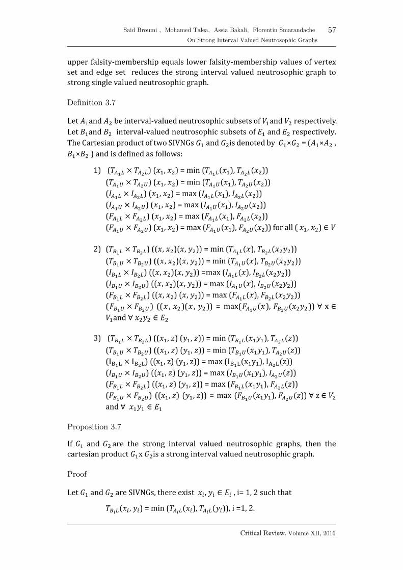
57
Critical Review. Volume XII, 2016
Said Broumi , Mohamed Talea, Assia Bakali, Florentin Smarandache .
On Strong Interval Valued Neutrosophic Graphs
upper falsity-membership equals lower falsity-membership values of vertex
set and edge set reduces the strong interval valued neutrosophic graph to
strong single valued neutrosophic graph.
Definition 3.7
Let 𝐴1and 𝐴2 be interval-valued neutrosophic subsets of 𝑉1and 𝑉2 respectively.
Let 𝐵1and 𝐵2 interval-valued neutrosophic subsets of 𝐸1 and 𝐸2 respectively.
The Cartesian product of two SIVNGs 𝐺1 and 𝐺2is denoted by 𝐺1×𝐺2 = (𝐴1×𝐴2 ,
𝐵1×𝐵2 ) and is defined as follows:
1) (𝑇𝐴1𝐿 × 𝑇𝐴2𝐿) (𝑥1, 𝑥2) = min (𝑇𝐴1𝐿(𝑥1), 𝑇𝐴2𝐿(𝑥2))
(𝑇𝐴1𝑈 × 𝑇𝐴2𝑈) (𝑥1, 𝑥2) = min (𝑇𝐴1𝑈(𝑥1), 𝑇𝐴2𝑈(𝑥2))
(𝐼𝐴1𝐿 × 𝐼𝐴2𝐿) (𝑥1, 𝑥2) = max (𝐼𝐴1𝐿(𝑥1), 𝐼𝐴2𝐿(𝑥2))
(𝐼𝐴1𝑈 × 𝐼𝐴2𝑈) (𝑥1, 𝑥2) = max (𝐼𝐴1𝑈(𝑥1), 𝐼𝐴2𝑈(𝑥2))
(𝐹𝐴1𝐿 × 𝐹𝐴2𝐿) (𝑥1, 𝑥2) = max (𝐹𝐴1𝐿(𝑥1), 𝐹𝐴2𝐿(𝑥2))
(𝐹𝐴1𝑈 × 𝐹𝐴2𝑈) (𝑥1, 𝑥2) = max (𝐹𝐴1𝑈(𝑥1), 𝐹𝐴2𝑈(𝑥2)) for all ( 𝑥1, 𝑥2) ∈ 𝑉
2) (𝑇𝐵1𝐿 × 𝑇𝐵2𝐿) ((𝑥, 𝑥2)(𝑥, 𝑦2)) = min (𝑇𝐴1𝐿(𝑥), 𝑇𝐵2𝐿(𝑥2𝑦2))
(𝑇𝐵1𝑈 × 𝑇𝐵2𝑈) ((𝑥, 𝑥2)(𝑥, 𝑦2)) = min (𝑇𝐴1𝑈(𝑥), 𝑇𝐵2𝑈(𝑥2𝑦2))
(𝐼𝐵1𝐿 × 𝐼𝐵2𝐿) ((𝑥, 𝑥2)(𝑥, 𝑦2)) =max (𝐼𝐴1𝐿(𝑥), 𝐼𝐵2𝐿(𝑥2𝑦2))
(𝐼𝐵1𝑈 × 𝐼𝐵2𝑈) ((𝑥, 𝑥2)(𝑥, 𝑦2)) = max (𝐼𝐴1𝑈(𝑥), 𝐼𝐵2𝑈(𝑥2𝑦2))
(𝐹𝐵1𝐿 × 𝐹𝐵2𝐿) ((𝑥, 𝑥2) (𝑥, 𝑦2)) = max (𝐹𝐴1𝐿(𝑥), 𝐹𝐵2𝐿(𝑥2𝑦2))
(𝐹𝐵1𝑈 × 𝐹𝐵2𝑈 ) ((𝑥 , 𝑥2 )(𝑥 , 𝑦2 )) = max(𝐹𝐴1𝑈(𝑥 ), 𝐹𝐵2𝑈(𝑥2𝑦2 )) ∀ x ∈
𝑉1and ∀ 𝑥2𝑦2 ∈ 𝐸2
3) (𝑇𝐵1𝐿 × 𝑇𝐵2𝐿) ((𝑥1, 𝑧) (𝑦1, 𝑧)) = min (𝑇𝐵1𝐿(𝑥1𝑦1), 𝑇𝐴2𝐿(𝑧))
(𝑇𝐵1𝑈 × 𝑇𝐵2𝑈) ((𝑥1, 𝑧) (𝑦1, 𝑧)) = min (𝑇𝐵1𝑈(𝑥1𝑦1), 𝑇𝐴2𝑈(𝑧))
(IB1L × IB2L) ((x1, z) (y1, z)) = max (IB1L(x1y1), IA2L(z))
(𝐼𝐵1𝑈 × 𝐼𝐵2𝑈) ((𝑥1, 𝑧) (𝑦1, 𝑧)) = max (𝐼𝐵1𝑈(𝑥1𝑦1), 𝐼𝐴2𝑈(𝑧))
(𝐹𝐵1𝐿 × 𝐹𝐵2𝐿) ((𝑥1, 𝑧) (𝑦1, 𝑧)) = max (𝐹𝐵1𝐿(𝑥1𝑦1), 𝐹𝐴2𝐿(𝑧))
(𝐹𝐵1𝑈 × 𝐹𝐵2𝑈) ((𝑥1, 𝑧) (𝑦1, 𝑧)) = max (𝐹𝐵1𝑈(𝑥1𝑦1), 𝐹𝐴2𝑈(𝑧)) ∀ z ∈ 𝑉2
and ∀ 𝑥1𝑦1 ∈ 𝐸1
Proposition 3.7
If 𝐺1 and 𝐺2 are the strong interval valued neutrosophic graphs, then the
cartesian product 𝐺1x 𝐺2is a strong interval valued neutrosophic graph.
Proof
Let 𝐺1 and 𝐺2 are SIVNGs, there exist 𝑥𝑖 , 𝑦𝑖 ∈ 𝐸𝑖 , i= 1, 2 such that
𝑇𝐵𝑖𝐿(𝑥𝑖, 𝑦𝑖) = min (𝑇𝐴𝑖𝐿(𝑥𝑖), 𝑇𝐴𝑖𝐿(𝑦𝑖)), i =1, 2.

58
Said Broumi, Mohamed Talea, Assia Bakali, Florentin Smarandache
On Strong Interval Valued Neutrosophic Graphs
Critical Review. Volume XII, 2016
𝑇𝐵𝑖𝑈(𝑥𝑖 , 𝑦𝑖) = min (𝑇𝐴𝑖𝑈(𝑥𝑖), 𝑇𝐴𝑖𝑈(𝑦𝑖)), i =1, 2.
𝐼𝐵𝑖𝐿(𝑥𝑖 , 𝑦𝑖) = max (𝐼𝐴𝑖𝐿(𝑥𝑖), 𝐼𝐴𝑖𝐿(𝑦𝑖)), i =1, 2.
𝐼𝐵𝑖𝑈(𝑥𝑖, 𝑦𝑖) = max (𝐼𝐴𝑖𝑈(𝑥𝑖), 𝐼𝐴𝑖𝑈(𝑦𝑖)), i =1, 2.
𝐹𝐵𝑖𝐿(𝑥𝑖 , 𝑦𝑖) = max (𝐹𝐴𝑖𝐿(𝑥𝑖), 𝐹𝐴𝑖𝐿(𝑦𝑖)), i =1, 2.
𝐹𝐵𝑖𝑈 (𝑥𝑖 , 𝑦𝑖) = max (𝐹𝐴𝑖𝑈(𝑥𝑖), 𝐹𝐴𝑖𝑈(𝑦𝑖)), i =1, 2.
Let E= {(𝑥, 𝑥2) (𝑥, 𝑦2) /𝑥 ∈ 𝑉1, 𝑥2𝑦2 ∈ 𝐸2}∪{(𝑥1, 𝑧) (𝑦1, 𝑧) /𝑧 ∈ 𝑉2, 𝑥1𝑦1 ∈ 𝐸1}.
Consider, (𝑥, 𝑥2) (𝑥, 𝑦2) ∈ 𝐸, we have
(𝑇𝐵1𝐿 × 𝑇𝐵2𝐿) ((𝑥, 𝑥2) (𝑥, 𝑦2)) = min (𝑇𝐴1𝐿(𝑥), 𝑇𝐵2𝐿(𝑥2𝑦2))
= min (𝑇𝐴1𝐿(𝑥), 𝑇𝐴2𝐿(𝑥2), 𝑇𝐴2𝐿(𝑦2))
Similarly,
(𝑇𝐵1𝑈 × 𝑇𝐵2𝑈) ((𝑥, 𝑥2) (𝑥, 𝑦2)) = min (𝑇𝐴1𝑈(𝑥), 𝑇𝐵2𝑈(𝑥2𝑦2))
= min (𝑇𝐴1𝑈(𝑥), 𝑇𝐴2𝑈(𝑥2), 𝑇𝐴2𝑈(𝑦2))
(𝑇𝐴1𝐿 × 𝑇𝐴2𝐿) (𝑥1, 𝑥2) = min (𝑇𝐴1𝐿(𝑥1), 𝑇𝐴2𝐿(𝑥2))
(𝑇𝐴1𝑈 × 𝑇𝐴2𝑈) (𝑥1, 𝑥2) = min (𝑇𝐴1𝑈(𝑥1), 𝑇𝐴2𝑈(𝑥2))
(𝑇𝐴1𝐿 × 𝑇𝐴2𝐿) (𝑥1, 𝑦2) = min (𝑇𝐴1𝐿(𝑥1), 𝑇𝐴2𝐿(𝑦2))
(𝑇𝐴1𝑈 × 𝑇𝐴2𝑈) (𝑥1, 𝑦2) = min (𝑇𝐴1𝑈(𝑥1), 𝑇𝐴2𝑈(𝑦2))
Min ((𝑇𝐴1𝑈 × 𝑇𝐴2𝑈) (𝑥, 𝑥2), (𝑇𝐴1𝑈 × 𝑇𝐴2𝑈) (𝑥, 𝑦2))
= min (min (𝑇𝐴1𝑈(𝑥), 𝑇𝐴2𝑈(𝑥2)), min (𝑇𝐴1𝑈(𝑥), 𝑇𝐴2𝑈(𝑦2)))
= min (𝑇𝐴1𝑈(𝑥), 𝑇𝐴2𝑈(𝑥2), 𝑇𝐴1𝑈(𝑦2))
Hence
(𝑇𝐵1𝐿 × 𝑇𝐵2𝐿) ((𝑥, 𝑥2) (𝑥, 𝑦2)) = min ((𝑇𝐴1𝐿 × 𝑇𝐴2𝐿) (𝑥, 𝑥2), (𝑇𝐴1𝐿 ×
𝑇𝐴2𝐿) (𝑥, 𝑦2))
(𝑇𝐵1𝑈 × 𝑇𝐵2𝑈) ((𝑥, 𝑥2) (𝑥, 𝑦2)) = min ((𝑇𝐴1𝑈 × 𝑇𝐴2𝑈) (𝑥, 𝑥2), (𝑇𝐴1𝑈 ×
𝑇𝐴2𝑈) (𝑥 ,𝑦2)).
Similarly, we can show that ―
(𝐼𝐵1𝐿 × 𝐼𝐵2𝐿) ((𝑥, 𝑥2) (𝑥, 𝑦2)) = max ((𝐼𝐴1𝐿 × 𝐼𝐴2𝐿) (𝑥, 𝑥2), (𝐼𝐴1𝐿 × 𝐼𝐴2𝐿)
(𝑥, 𝑦2))
(𝐼𝐵1𝑈 × 𝐼𝐵2𝑈) ((𝑥, 𝑥2) (𝑥, 𝑦2)) = max ((𝐼𝐴1𝑈 × 𝐼𝐴2𝑈) (𝑥, 𝑥2), (𝐼𝐴1𝑈 ×
𝐼𝐴2𝑈) (𝑥, 𝑦2)).
And also

59
Critical Review. Volume XII, 2016
Said Broumi , Mohamed Talea, Assia Bakali, Florentin Smarandache .
On Strong Interval Valued Neutrosophic Graphs
(𝐹𝐵1𝐿 × 𝐹𝐵2𝐿) ((𝑥, 𝑥2) (𝑥, 𝑦2)) = max ((𝐹𝐴1𝐿 × 𝐹𝐴2𝐿) (𝑥, 𝑥2), (𝐹𝐴1𝐿 ×
𝐹𝐴2𝐿) (𝑥, 𝑦2))
(𝐹𝐵1𝑈 × 𝐹𝐵2𝑈) ((𝑥, 𝑥2) (𝑥, 𝑦2)) = max ((𝐹𝐴1𝑈 × 𝐹𝐴2𝑈) (𝑥, 𝑥2), (𝐹𝐴1𝑈 ×
𝐹𝐴2𝑈) (𝑥, 𝑦2)).
Hence, 𝐺1x 𝐺2 strong interval valued neutrosophic graph. This completes the
proof.
Proposition 3.8
If 𝐺1 x 𝐺2 is strong interval valued neutrosophic graph, then at least 𝐺1 or
𝐺2must be strong.
Proof
Let 𝐺1 and 𝐺2 be no strong interval valued neutrosophic graphs; there exists
𝑥𝑖 , 𝑦𝑖 ∈ 𝐸𝑖 , I = 1, 2, such that
𝑇𝐵𝑖𝐿(𝑥𝑖, 𝑦𝑖) < min (𝑇𝐴𝑖𝐿(𝑥𝑖), 𝑇𝐴𝑖𝐿(𝑦𝑖)), i =1, 2.
𝑇𝐵𝑖𝑈(𝑥𝑖 , 𝑦𝑖) < min (𝑇𝐴𝑖𝑈(𝑥𝑖), 𝑇𝐴𝑖𝑈(𝑦𝑖)), i =1, 2.
𝐼𝐵𝑖𝐿(𝑥𝑖 , 𝑦𝑖) > max (𝐼𝐴𝑖𝐿(𝑥𝑖), 𝐼𝐴𝑖𝐿(𝑦𝑖)), i =1, 2.
𝐼𝐵𝑖𝑈(𝑥𝑖, 𝑦𝑖) > max (𝐼𝐴𝑖𝑈(𝑥𝑖), 𝐼𝐴𝑖𝑈(𝑦𝑖)), i =1, 2.
𝐹𝐵𝑖𝐿(𝑥𝑖 , 𝑦𝑖) > max (𝐹𝐴𝑖𝐿(𝑥𝑖), 𝐹𝐴𝑖𝐿(𝑦𝑖)), i =1, 2.
𝐹𝐵𝑖𝑈 (𝑥𝑖 , 𝑦𝑖) > max (𝐹𝐴𝑖𝑈(𝑥𝑖), 𝐹𝐴𝑖𝑈(𝑦𝑖)), i =1, 2.
Let E= {(𝑥, 𝑥2) (𝑥, 𝑦2) /𝑥 ∈ 𝑉1, 𝑥2𝑦2 ∈ 𝐸2}∪{(𝑥1, 𝑧) (𝑦1, 𝑧) /𝑧 ∈ 𝑉2, 𝑥1𝑦1 ∈ 𝐸1}
Consider, (𝑥, 𝑥2) (𝑥, 𝑦2) ∈ 𝐸, we have
(𝑇𝐵1𝐿 × 𝑇𝐵2𝐿) ((𝑥, 𝑥2) (𝑥, 𝑦2)) = min (𝑇𝐴1𝐿(𝑥), 𝑇𝐵2𝐿(𝑥2𝑦2))
< min (𝑇𝐴1𝐿(𝑥), 𝑇𝐴2𝐿(𝑥2), 𝑇𝐴2𝐿(𝑦2)).
Similarly ―
(𝑇𝐵1𝑈 × 𝑇𝐵2𝑈) ((𝑥, 𝑥2) (𝑥, 𝑦2)) = min (𝑇𝐴1𝑈(𝑥), 𝑇𝐵2𝑈(𝑥2𝑦2))
< min (𝑇𝐴1𝑈(𝑥), 𝑇𝐴2𝑈(𝑥2), 𝑇𝐴2𝑈(𝑦2))
(𝑇𝐴1𝐿 × 𝑇𝐴2𝐿) (𝑥1, 𝑥2) = min (𝑇𝐴1𝐿(𝑥1), 𝑇𝐴2𝐿(𝑥2))
(𝑇𝐴1𝑈 × 𝑇𝐴2𝑈) (𝑥1, 𝑥2) = min (𝑇𝐴1𝑈(𝑥1), 𝑇𝐴2𝑈(𝑥2))
(𝑇𝐴1𝐿 × 𝑇𝐴2𝐿) (𝑥1, 𝑦2) = min (𝑇𝐴1𝐿(𝑥1), 𝑇𝐴2𝐿(𝑦2))
(𝑇𝐴1𝑈 × 𝑇𝐴2𝑈) (𝑥1, 𝑦2) = min (𝑇𝐴1𝑈(𝑥1), 𝑇𝐴2𝑈(𝑦2))
min ((𝑇𝐴1𝑈 × 𝑇𝐴2𝑈) (𝑥, 𝑥2), (𝑇𝐴1𝑈 × 𝑇𝐴2𝑈) (𝑥, 𝑦2))
= min (min (𝑇𝐴1𝑈(𝑥), 𝑇𝐴2𝑈(𝑥2)), min (𝑇𝐴1𝑈(𝑥), 𝑇𝐴2𝑈(𝑦2)))
= min (𝑇𝐴1𝑈(𝑥), 𝑇𝐴2𝑈(𝑥2), 𝑇𝐴1𝑈(𝑦2)).

60
Said Broumi, Mohamed Talea, Assia Bakali, Florentin Smarandache
On Strong Interval Valued Neutrosophic Graphs
Critical Review. Volume XII, 2016
Hence
(𝑇𝐵1𝐿 × 𝑇𝐵2𝐿) ((𝑥, 𝑥2) (𝑥, 𝑦2)) < min ((𝑇𝐴1𝐿 × 𝑇𝐴2𝐿) (𝑥, 𝑥2), (𝑇𝐴1𝐿 ×
𝑇𝐴2𝐿) (𝑥, 𝑦2)),
(𝑇𝐵1𝑈 × 𝑇𝐵2𝑈) ((𝑥, 𝑥2) (𝑥, 𝑦2)) < min ((𝑇𝐴1𝑈 × 𝑇𝐴2𝑈) (𝑥, 𝑥2), (𝑇𝐴1𝑈 ×
𝑇𝐴2𝑈) (𝑥 ,𝑦2)).
Similarly, we can show that
(𝐼𝐵1𝐿 × 𝐼𝐵2𝐿) ((𝑥, 𝑥2) (𝑥, 𝑦2)) > max ((𝐼𝐴1𝐿 × 𝐼𝐴2𝐿) (𝑥, 𝑥2), (𝐼𝐴1𝐿 × 𝐼𝐴2𝐿)
(𝑥, 𝑦2)),
(𝐼𝐵1𝑈 × 𝐼𝐵2𝑈) ((𝑥, 𝑥2) (𝑥, 𝑦2)) > max ((𝐼𝐴1𝑈 × 𝐼𝐴2𝑈) (𝑥, 𝑥2), (𝐼𝐴1𝑈 ×
𝐼𝐴2𝑈) (𝑥, 𝑦2)).
And also
(𝐹𝐵1𝐿 × 𝐹𝐵2𝐿) ((𝑥, 𝑥2) (𝑥, 𝑦2)) > max ((𝐹𝐴1𝐿 × 𝐹𝐴2𝐿) (𝑥, 𝑥2), (𝐹𝐴1𝐿 ×
𝐹𝐴2𝐿) (𝑥, 𝑦2)),
(𝐹𝐵1𝑈 × 𝐹𝐵2𝑈) ((𝑥, 𝑥2) (𝑥, 𝑦2)) > max ((𝐹𝐴1𝑈 × 𝐹𝐴2𝑈) (𝑥, 𝑥2), (𝐹𝐴1𝑈 ×
𝐹𝐴2𝑈) (𝑥, 𝑦2)).
Hence, 𝐺1 x 𝐺2 is not strong interval valued neutrosophic graph, which is a
contradiction. This completes the proof.
Remark 3.9
If 𝐺1is a SIVNG and 𝐺2 is not a SIVNG, then 𝐺1 x 𝐺2 is need not be an SIVNG.
Example 3.10
Let 𝐺1= (𝐴1,𝐵1) be a SIVNG, where 𝐴1= {< a, [0.6, 0.7], [0.2, 0.5], [0.1, 0.3]> ,< b,
[0.6, 0.7], [0.2, 0.5], [0.1, 0.3]>} and 𝐵1= {< ab, [0.6, 0.7], [0.2, 0.5], [0.1, 0.3]>}
Figure 5. Interval valued neutrosophic 𝐺1.
𝐺2= (𝐴2,𝐵2) is not a SIVNG, where 𝐴2= {< c, [0.4, 0.6], [0.2, 0.4], [0.1, 0.3]>, < d,
[0.4, 0.6], [0.1,0.3], [0.2, 0.4] >} and 𝐵2= < cd, [0.3,0.5], [0.1, 0.2], [0.3, 0.5]>}.
Figure 6. Interval valued neutrosophic 𝐺2.
𝑎
<[0.6, 0.7],[ 0.2, 0.5],[0.1, 0.3]> <[0.6, 0.7],[ 0.2, 0.5],[0.1, 0.3]>
<[0.6, 0.7],[ 0.2, 0.5],[0.1, 0.3]>
𝑏 𝐺1
𝑐
<[0.4, 0.6],[ 0.2, 0.4],[0.1, 0.3]> <[0.4, 0.6],[ 0.1, 0.3],[0.2, 0.4]>
<[0.3, 0.5],[ 0.1, 0.3],[0.3, 0.5]>
𝑑 𝐺2

61
Critical Review. Volume XII, 2016
Said Broumi , Mohamed Talea, Assia Bakali, Florentin Smarandache .
On Strong Interval Valued Neutrosophic Graphs
𝐺1x 𝐺2= (𝐴1x 𝐴2, 𝐵1x 𝐵2) is not a SIVNG, where
𝐴1x 𝐴2= {< (a, c), [0.4, 0.6],[ 0.2, 0.3], [0.2, 0.4]>, < (a, d), [0.4, 0.6], [0.2, 0.3],
[0.2, 0.4]>, < (b, c), [0.4, 0.6], [0.2, 0.6], [0.2, 0.4]>, < (b, d), [0.4, 0.6], [0.3, 0.4],
[0.2, 0.4]>},
𝐵1x 𝐵2= {< ((a, c), (a, d)), [0.3, 0.5], [0.3, 0.5], [0.3, 0.5] >, < ((a, c), (b, c)), [0.4,
0.6], [0.1, 0.4], [0.3, 0.4] >, < ((b, c), (b, d)), [0.4, 0.6], [0.2, 0.4], [0.2, 0.4] >, <
((a, d), (b, d)),[0.4, 0.6], [0.2, 0.4], [0.2, 0.4] >}. In this example, 𝐺1 is a SIVNG
and 𝐺2is not a SIVNG, then 𝐺1x 𝐺2is not a SIVNG.
Figure 7. Cartesian product 𝐺1x 𝐺2
Example 3.11
Let 𝐺1= (𝐴1, 𝐵1) be a SIVNG, where 𝐴1= {< a, [0.4, 0.6], [0.2, 0.4], [0.1, 0.3] >, <
b, [0.4, 0.6], [0.2, 0.4], [0.1, 0.3]>} and 𝐵1={< ab, [0.4, 0.6], [0.2, 0.4], [0.1, 0.3] >,
Figure 8. Interval valued neutrosophic 𝐺1.
𝐺2= (𝐴2, 𝐵2) is not a SIVIFG, where 𝐴2= {< c, [0.6, 0.7], [0.1, 0.3], [0.1, 0.3] >, <
d, [0.6, 0.7], [0.1, 0.3], [0.2, 0.4] >} and 𝐵2= {< cd, [0.5, 0.6], [0.2, 0.4], [0.2, 0.4]>},
Figure 9. Interval valued neutrosophic 𝐺2.
𝐺1x 𝐺2= (𝐴1x 𝐴2, 𝐵1x 𝐵2) is a SIVNG, where
<a, [.4, .6], [.2, .4], [.1, .3]> <b, [.4, .6], [.2, .4], [.1, .3]>
<ab, [.4, .6], [.2, .4], [.1, .3]> 𝐺1
<c, [.6, .7], [.1, .3], [.1, .3]> <d, [.6, .7], [.1, .3], [.2, .4]>
<cd, [.5, .6], [.2, .4], [.2, .4]> 𝐺2
𝑎𝑑
<[0.4, 0.6],[ 0.3, 0.4],[0.2, 0.4]>
<[0.4, 0.6],[ 0.2, 0.4],[01, 0.3]>
𝑏𝑑
<[0.4, 0.6],[ 0.2, 0.3],[0.2, 0.4]>
<[0
.3, 0
.5],
[ 0
.3, 0
.5],
[0.3
, 0.5
]>
<[0.4, 0.6],[ 0.2, 0.6],[0.2, 0.4]> <[0.4, 0.6],[ 0.2, 0.3],[0.2, 0.4]>
𝑎𝑐
<[0.4, 0.6],[ 0.1, 0.4],[0.3, 0.4]>
𝑏𝑐
<[0
.4, 0
.6],
[ 0
.2, 0
.4,[
0.2
, 0.4
]>

62
Said Broumi, Mohamed Talea, Assia Bakali, Florentin Smarandache
On Strong Interval Valued Neutrosophic Graphs
Critical Review. Volume XII, 2016
𝐴1x 𝐴2= {< (a, c), [0.4, 0.6], [0.2, 0.4], [0.1, 0.3] >, < (a, d), [0.4, 0.6], [0.2, 0.4],
[0.2, 0.4] >, < (b, c), [0.4, 0.6], [0.2, 0.4], [0.1, 0.3] >, < (b, d), [0.4, 0.6], [0.2,
0.4], [0.2, 0.4] >} and
𝐵1x 𝐵2= {< ((a, c), (a, d)), [0.4, 0.6], [0.2, 0.4], [0.2, 0.4] >, < ((a, c), (b, c)), [0.4,
0.6], [0.2, 0.4], [0.1, 0.3] >, < ((b, c), (b, d)), [0.4, 0.6], [0.2, 0.4], [0.2, 0.4] >, <
((a, d), (b, d)), [0.4, 0.6], [0.2, 0.4], [0.2, 0.4]>}. In this example, 𝐺1is a SIVNG
and 𝐺2is not a SIVNG, then 𝐺1x 𝐺2is a SIVNG.
Figure 10. Cartesian product
Proposition 3.12
Let 𝐺1be a strong interval valued neutrosophic graph. Then for any interval
valued neutrosophic graph 𝐺2,𝐺1x 𝐺2 is strong interval valued neutrosophic
graph iff
𝑇𝐴1𝐿(𝑥1) ≤ 𝑇𝐵1𝐿(𝑥2𝑦2), 𝐼𝐴1𝐿(𝑥1) ≥ 𝐼𝐵1𝐿(𝑥2𝑦2) and 𝐹𝐴1𝐿(𝑥1) ≥
𝐹𝐵1𝐿(𝑥2𝑦2),
𝑇𝐴1𝑈(𝑥1) ≤ 𝑇𝐵1𝑈(𝑥2𝑦2), 𝐼𝐴1𝑈(𝑥1) ≥ 𝐼𝐵1𝑈(𝑥2𝑦2) and 𝐹𝐴1𝑈(𝑥1) ≥
𝐹𝐵1𝑈(𝑥2𝑦2), ∀ 𝑥1 ∈ 𝑉1 ,𝑥2𝑦2 ∈ 𝐸2.
Definition 3.13
Let 𝐴1and 𝐴2be interval valued neutrosophic subsets of 𝑉1and 𝑉2respectively.
Let 𝐵1and 𝐵2 interval-valued neutrosophic subsets of 𝐸1 and 𝐸2 respectively.
The composition of two strong interval valued neutrosophic graphs 𝐺1 and
𝐺2is denoted by 𝐺1[ 𝐺2] = (𝐴1 ∘ 𝐴2, 𝐵1 ∘ 𝐵2 ) and is defined as follows
1) (𝑇𝐴1𝐿 ∘ 𝑇𝐴2𝐿) (𝑥1, 𝑥2) = min (𝑇𝐴1𝐿(𝑥1), 𝑇𝐴2𝐿(𝑥2))
(𝑇𝐴1𝑈 ∘ 𝑇𝐴2𝑈) (𝑥1, 𝑥2) = min (𝑇𝐴1𝑈(𝑥1), 𝑇𝐴2𝑈(𝑥2))
(𝐼𝐴1𝐿 ∘ 𝐼𝐴2𝐿) (𝑥1, 𝑥2) = max (𝐼𝐴1𝐿(𝑥1), 𝐼𝐴2𝐿(𝑥2))
(𝐼𝐴1𝑈 ∘ 𝐼𝐴2𝑈) (𝑥1, 𝑥2) = max (𝐼𝐴1𝑈(𝑥1), 𝐼𝐴2𝑈(𝑥2))
<ad, [.4, .6], [.2, .4],[.2, .4]>
<bc, [.4, .6], [.2, .4],[.1, .3]>
<bd, [.4, .6], [.2, .4],[.2, .4]>
<ac, [.4, .6], [.2, .4],[.1, .3]> <(ac,bc), [.4, .6], [.2, .4],[.1, .3]>
<(b
d,b
c), [.
4, .6
], [
.2, .4
],[.
2 .
4]>
<(ad,bd), [.4, .6], [.2, .4],[.2, .4]>
<(a
d,a
c), [.
4, .6
], [
.2, .4
],[.
2.4
]>

63
Critical Review. Volume XII, 2016
Said Broumi , Mohamed Talea, Assia Bakali, Florentin Smarandache .
On Strong Interval Valued Neutrosophic Graphs
(𝐹𝐴1𝐿 ∘ 𝐹𝐴2𝐿) (𝑥1, 𝑥2) = max (𝐹𝐴1𝐿(𝑥1), 𝐹𝐴2𝐿(𝑥2))
(𝐹𝐴1𝑈 ∘ 𝐹𝐴2𝑈) (𝑥1, 𝑥2) = max (𝐹𝐴1𝑈(𝑥1), 𝐹𝐴2𝑈(𝑥2)) ∀ 𝑥1 ∈ 𝑉1, 𝑥2 ∈ 𝑉2
2) (𝑇𝐵1𝐿 ∘ 𝑇𝐵2𝐿) ((𝑥, 𝑥2)(𝑥, 𝑦2)) = min (𝑇𝐴1𝐿(𝑥), 𝑇𝐵2𝐿(𝑥2𝑦2))
(𝑇𝐵1𝑈 ∘ 𝑇𝐵2𝑈) ((𝑥, 𝑥2)(𝑥, 𝑦2)) = min (𝑇𝐴1𝑈(𝑥), 𝑇𝐵2𝑈(𝑥2𝑦2))
(𝐼𝐵1𝐿 ∘ 𝐼𝐵2𝐿) ((𝑥, 𝑥2)(𝑥, 𝑦2)) = max (𝐼𝐴1𝐿(𝑥), 𝐼𝐵2𝐿(𝑥2𝑦2))
(𝐼𝐵1𝑈 ∘ 𝐼𝐵2𝑈) ((𝑥, 𝑥2)(𝑥, 𝑦2)) = max (𝐼𝐴1𝑈(𝑥), 𝐼𝐵2𝑈(𝑥2𝑦2))
(𝐹𝐵1𝐿 ∘ 𝐹𝐵2𝐿) ((𝑥, 𝑥2) (𝑥, 𝑦2)) = max (𝐹𝐴1𝐿(𝑥), 𝐹𝐵2𝐿(𝑥2𝑦2))
(𝐹𝐵1𝑈 ∘ 𝐹𝐵2𝑈 ) ((𝑥 , 𝑥2 )(𝑥 , 𝑦2 )) = max (𝐹𝐴1𝑈(𝑥), 𝐹𝐵2𝑈(𝑥2𝑦2 )) ∀ 𝑥 ∈
𝑉1, ∀ 𝑥2𝑦2 ∈ 𝐸2
3) (𝑇𝐵1𝐿 ∘ 𝑇𝐵2𝐿) ((𝑥1, 𝑧) (𝑦1, 𝑧)) = min (𝑇𝐵1𝐿(𝑥1𝑦1), 𝑇𝐴2𝐿(𝑧))
(𝑇𝐵1𝑈 ∘ 𝑇𝐵2𝑈) ((𝑥1, 𝑧) (𝑦1, 𝑧)) = min (𝑇𝐵1𝑈(𝑥1𝑦1), 𝑇𝐴2𝑈(𝑧))
(IB1L ∘ IB2L) ((x1, z) (y1, z)) = max (IB1L(x1y1), IA2L(z))
(IB1U ∘ IB2U) ((x1, z) (y1, z)) = max (IB1U(x1y1), IA2U(z))
(FB1L ∘ FB2L) ((x1, z) (y1, z)) = max (FB1L(x1y1), FA2L(z))
(FB1U ∘ FB2U) ((x1, z) (y1, z)) = max (FB1U(x1y1), FA2U(z)) ∀ z ∈ V2, ∀
x1y1 ∈ E1
4) ( TB1L ∘ TB2L ) (( x1 , x2 ) ( y1 , y2 )) = min ( TA2L(x2 ), TA2L(y2 ),
TB1L(x1y1))
( 𝑇𝐵1𝑈 ∘ 𝑇𝐵2𝑈 ) (( 𝑥1 , 𝑥2 ) ( 𝑦1 , 𝑦2 )) = min ( 𝑇𝐴2𝑈(𝑥2 ), 𝑇𝐴2𝑈(𝑦2 ),
𝑇𝐵1𝑈(𝑥1𝑦1))
(𝐼𝐵1𝐿 ∘ 𝐼𝐵2𝐿) ((𝑥1, 𝑥2) (𝑦1, 𝑦2)) = max(𝐼𝐴2𝐿(𝑥2), 𝐼𝐴2𝐿(𝑦2), 𝐼𝐵1𝐿(𝑥1𝑦1))
(𝐼𝐵1𝑈 ∘ 𝐼𝐵2𝑈) ((𝑥1, 𝑥2) (𝑦1, 𝑦2))= max (𝐼𝐴2𝑈(𝑥2), 𝐼𝐴2𝑈(𝑦2), 𝐼𝐵1𝑈(𝑥1𝑦1))
(𝐹𝐵1𝐿 ∘ 𝐹𝐵2𝐿) ((𝑥1, 𝑥2) (𝑦1, 𝑦2)) = max(𝐹𝐴2𝐿(𝑥2), 𝐹𝐴2𝐿(𝑦2), 𝐹𝐵1𝐿(𝑥1𝑦1))
( 𝐹𝐵1𝑈 ∘ 𝐹𝐵2𝑈 )(( 𝑥1 , 𝑥2 ) ( 𝑦1 , 𝑦2 )) = max ( 𝐹𝐴2𝑈(𝑥2 ), 𝐹𝐴2𝑈(𝑦2 ),
𝐹𝐵1𝑈(𝑥1𝑦1))
∀( 𝑥1 , 𝑥2)( 𝑦1 , 𝑦2) ∈ 𝐸0 -E , where 𝐸0 = E ∪ { ( 𝑥1 , 𝑥2) ( 𝑦1 , 𝑦2)
|𝑥1𝑦1 ∈ 𝐸1, 𝑥2 ≠ 𝑦2}.
The following propositions are stated without their proof.
Proposition 3.14
If 𝐺1 and 𝐺2 are the strong interval valued neutrosophic graphs, then the
composition 𝐺1[ 𝐺2] is a strong interval valued neutrosophic graph.
Proposition 3.15
If 𝐺1[ 𝐺2] is strong interval valued neutrosophic graphs, then at least
composition 𝐺1 or 𝐺2 must be strong.

64
Said Broumi, Mohamed Talea, Assia Bakali, Florentin Smarandache
On Strong Interval Valued Neutrosophic Graphs
Critical Review. Volume XII, 2016
Example 3.16
Let 𝐺1= (𝐴1,𝐵1) be a SIVNG, where 𝐴1= {< a, [0.6, 0.7], [0.2, 0.3], [0.1, 0.3], > ,<
b, [0.6, 0.7], [0.2, 0.3], [0.1, 0.3] >} and 𝐵1= {< ab, [0.6, 0.7], [0.2, 0.3], [0.1, 0.3]>}.
Figure 11. Interval valued neutrosophic 𝐺1.
𝐺2= (𝐴2,𝐵2) is not a SIVNG, where 𝐴2= {< c, [0.4, 0.6], [0.2, 0.4], [0.1, 0.3] >, <
d, [0.4, 0.6], [0.2, 0.4], [0.1, 0.3] >} and 𝐵2=<cd, [0.3, 0.5], [0.2, 0.5], [0.3, 0.5]>}.
Figure 12. Interval valued neutrosophic 𝐺2.
𝐺1[𝐺2]= (𝐴1o𝐴2, 𝐵1o𝐵2) is not a SIVNG, where
𝐴1o𝐴2= {< (a,c), [0.4, 0.6], [0.2, 0.4], [0.1, 0.3] >, < (a,d), [0.4, 0.6], [0.2, 0.4],
[0.1, 0.3] >, < (b, c), [0.4, 0.6], [0.2, 0.4], [0.1, 0.3] >, < (b, d), [0.4, 0.6], [0.2, 0.4],
[0.1, 0.3] >},
𝐵1o𝐵2= {< ((a, c), (a, d)), [0.3, 0.5], [0.2, 0.4], [0.3, 0.5] >, < ((a, c), (b, c)), [0.4,
0.6], [0.2, 0.4], [0.1, 0.3]>, < ((b, c), (b, d)),[0.3, 0.5], [0.2, 0.4], [0.3, 0.5] >, < ((a,
d), (b, d)), [0.4, 0.6], [0.2, 0.4], [0.1, 0.3] >, < ((a, c), (b, d)), [0.4, 0.6], [0.2, 0.4],
[0.1, 0.3] >, < ((a, d), (b, c)), [0.4, 0.6], [0.2, 0.4], [0.1, 0.3] >}. In this example, 𝐺1
is a SIVNG and 𝐺2is not a SIVNG, then 𝐺1[𝐺2] is not a SIVNG.
Figure 13. Composition
<ad, [.4, .6], [.2, .4],[.1, .3]>
<bc, [.4, .6], [.2, .4],[.1, .3]>
<bd, [.4, .6], [.2, .4],[.1, .3]>
<ac, [.4, .6], [.2, .4],[.1, .3]> <(ac,bc), [.4, .6], [.2, .4],[.1, .3]>
<(b
d,b
c), [.
3, .5
], [
.2, .4
],[.
3,
.5]>
<(ac,bd), [.4, .6], [.2, .4],[.1, .3]>
<(ad,bd), [.4, .6], [.2, .4],[.1, .3]>
<(a
d,a
c), [.
3, .5
], [
.2, .4
],[.
3,
.5]>
<(ad,bc), [.4, .6], [.2, .4],[.1, .3]>
<a, [.6, .7], [.2, .3],[.1, .3]> <b, [.6, .7], [.2, .3],[.1, .3]>
<ab, [.6, .7], [.2, .3],[.1, .3]> 𝐺1
<c, [.4, .6], [.2, .4], [.1, .3]> <d, [.4, .6], [.2, .4], [.1, .3]>
<cd, [.3, .5], [.2, .4], [.3, .5]> 𝐺2

65
Critical Review. Volume XII, 2016
Said Broumi , Mohamed Talea, Assia Bakali, Florentin Smarandache .
On Strong Interval Valued Neutrosophic Graphs
Example 3.17
Let 𝐺1= (𝐴1,𝐵1) be a SIVNG, where 𝐴1= {< a, [0.4, 0.6], [0.2, 0.4], [0.2, 0.4] >, <
b, [0.4, 0.6], [0.2, 0.4], [0.2, 0.4] >}and 𝐵1={<ab, [0.4, 0.6], [0.2, 0.4], [0.2, 0.4] >}.
Figure 14. Interval valued neutrosophic 𝐺1.
𝐺2= (𝐴2,𝐵2) is not a SIVNG, where 𝐴2= {< c, [0.6, 0.7], [0.1, 0.3], [0.1, 0.3] >, <d,
[0.6, 0.7], [0.2, 0.4], [0.1, 0.3] >} and 𝐵2={< c d, [0.5, 0.6], [0.2, 0.4], [0.2, 0.4] >}.
Figure 15. Interval valued neutrosophic 𝐺2.
𝐺1[𝐺2] = (𝐴1o𝐴2, 𝐵1 o𝐵2) is a SIVNG, where
𝐴1o𝐴2= {< (a, c), [0.4, 0.6], [0.2, 0.4], [0.2, 0.4] >, < (a, d), [0.4, 0.6], [0.2, 0.4],
[0.2, 0.4] >, < (b, c), [0.4, 0.6], [0.2, 0.4], [0.2, 0.4] >, < (b, d), [0.4, 0.6], [0.2,
0.4],[0.2, 0.4] >} and
𝐵1 o𝐵2= {< ((a, c), (a, d)), [0.4, 0.6], [0.2, 0.4] [0.2, 0.4] >, < ((a, c), (b, c)), [0.4,
0.6], [0.2, 0.4], [0.2, 0.4] >, < ((b, c), (b, d)), [0.4, 0.6], [0,2, 0.4] [0.2, 0.4] >, < ((a,
d), (b, d)), [0.4, 0.6], [0.2, 0.4], [0.2, 0.4] >, < ((a, c), (b, d)), [0.4, 0.6], [0.2, 0.4]
[0.2, 0.4]>, < ((a, d), (b, c)), [0.4, 0.6], [0.2, 0.4], [0.2, 0.4]>}. In this example, 𝐺1is
an SIVIFG and 𝐺2is not a SIVNG, then 𝐺1[𝐺2] is a SIVNG.
Figure 16. Composition of 𝐺1 and 𝐺2.
<a, [.4, .6], [.2, .4], [.2, .4]> <b, [.4, .6], [.2, .4], [.2, .4]>
<ab, [.4, .6], [.2, .4], [.2, .4]>
𝐺1
<c, [.6, .7], [.1, .3], [.1, .3]> <d, [.6, .7], [.2, .4], [.1, .3]>
<cd, [.5, .6], [.2, .4], [.2, .4]> 𝐺2
<ad, [.4, .6], [.2, .4],[.2, .4]>
<bc, [.4, .6], [.2, .4],[.2, .4]>
<bd, [.4, .6], [.2, .4],[.2, .4]>
<ac, [.4, .6], [.2, .4],[.2, .4]> <(ac,bc), [.4, .6], [.2, .4],[.2, .4]>
<(b
d,b
c), [.
4 .6
], [
.2, .4
],[.
2,
.4]>
<(ac,bd), [.4, .6], [.2, .4],[.2, .4]>
<(ad,bd), [.4, .6], [.2, .4],[.2, .4]>
<(a
d,a
c), [.
4, .6
], [
.2, .4
],[.
2,
.4]>
<(ad,bc), [.4, .6], [.2, .4],[.2, .4]>

66
Said Broumi, Mohamed Talea, Assia Bakali, Florentin Smarandache
On Strong Interval Valued Neutrosophic Graphs
Critical Review. Volume XII, 2016
Proposition 3.18
Let 𝐺1be a strong interval valued neutrosophic graph. Then for any interval valued
neutrosophic graph 𝐺2,𝐺1[𝐺2] is strong interval valued neutrosophic graph iff ―
𝑇𝐴1𝐿(𝑥1) ≤ 𝑇𝐵1𝐿(𝑥2𝑦2), 𝐼𝐴1𝐿(𝑥1) ≥ 𝐼𝐵1𝐿(𝑥2𝑦2) and 𝐹𝐴1𝐿(𝑥1) ≥
𝐹𝐵1𝐿(𝑥2𝑦2),
𝑇𝐴1𝑈(𝑥1) ≤ 𝑇𝐵1𝑈(𝑥2𝑦2), 𝐼𝐴1𝑈(𝑥1) ≥ 𝐼𝐵1𝑈(𝑥2𝑦2) and 𝐹𝐴1𝑈(𝑥1) ≥
𝐹𝐵1𝑈(𝑥2𝑦2), ∀ 𝑥1 ∈ 𝑉1 ,𝑥2𝑦2 ∈ 𝐸2.
Definition 3.19
Let A1and A2 be interval valued neutrosophic subsets of V1and V2 respectively.
Let B1and B1 interval valued neutrosophic subsets of E1 and E2 respectively.
The join of two strong interval valued neutrosophic graphs G1 and G2 is
denoted by G1 + G2= (A1 + A2, B1 + B2) and is defined as follows
1) (𝑇𝐴1𝐿 + 𝑇𝐴2𝐿)(𝑥) ={
(𝑇𝐴1𝐿 ∪ 𝑇𝐴2𝐿)(𝑥) if 𝑥 ∈ 𝑉1 ∪ 𝑉2
𝑇𝐴1𝐿(𝑥) if 𝑥 ∈ 𝑉1
𝑇𝐴2𝐿(𝑥) if 𝑥 ∈ 𝑉2
(𝑇𝐴1𝑈 + 𝑇𝐴2𝑈)(𝑥) = {
(𝑇𝐴1𝑈 ∪ 𝑇𝐴2𝑈)(𝑥) if 𝑥 ∈ 𝑉1 ∪ 𝑉2
𝑇𝐴1𝑈(𝑥) if 𝑥 ∈ 𝑉1
𝑇𝐴2𝑈(𝑥) if 𝑥 ∈ 𝑉2
(𝐼𝐴1𝐿 + 𝐼𝐴2𝐿) (𝑥) = {
(𝐼𝐴1𝐿 ∩ 𝐼𝐴2𝐿)(𝑥) if 𝑥 ∈ 𝑉1 ∪ 𝑉2
𝐼𝐴1𝐿(𝑥) if 𝑥 ∈ 𝑉1
𝐼𝐴2𝐿(𝑥) if 𝑥 ∈ 𝑉2
(𝐼𝐴1𝑈 + 𝐼𝐴2𝑈) (𝑥) = {
(𝐼𝐴1𝑈 ∩ 𝐼𝐴2𝑈)(𝑥) if 𝑥 ∈ 𝑉1 ∪ 𝑉2
𝐼𝐴1𝑈(𝑥) if 𝑥 ∈ 𝑉1
𝐼𝐴2𝑈(𝑥) if 𝑥 ∈ 𝑉2
(𝐹𝐴1𝐿 + 𝐹𝐴2𝐿) (𝑥) = {
(𝐹𝐴1𝐿 ∩ 𝐹𝐴2𝐿)(𝑥) if 𝑥 ∈ 𝑉1 ∪ 𝑉2
𝐹𝐴1𝐿(𝑥) if 𝑥 ∈ 𝑉1
𝐹𝐴2𝐿(𝑥) if 𝑥 ∈ 𝑉2
(𝐹𝐴1𝑈 + 𝐹𝐴2𝑈) (𝑥) = {
(𝐹𝐴1𝑈 ∩ 𝐹𝐴2𝑈)(𝑥) if 𝑥 ∈ 𝑉1 ∪ 𝑉2
𝐹𝐴1𝑈(𝑥) if 𝑥 ∈ 𝑉1
𝐹𝐴2𝑈(𝑥) if 𝑥 ∈ 𝑉2
2) (𝑇𝐵1𝐿 + 𝑇𝐵2𝐿) (𝑥y) = {
(𝑇𝐵1𝐿 ∪ 𝑇𝐵2𝐿)(xy) if 𝑥𝑦 ∈ 𝐸1 ∪ 𝐸2
𝑇𝐵1𝐿(𝑥𝑦) if 𝑥𝑦 ∈ 𝐸1
𝑇𝐵2𝐿(𝑥𝑦) if 𝑥𝑦 ∈ 𝐸2
(𝑇𝐵1𝑈 + 𝑇𝐵2𝑈) (𝑥y) ={
(𝑇𝐵1𝑈 ∪ 𝑇𝐵2𝑈)(xy) if 𝑥𝑦 ∈ 𝐸1 ∪ 𝐸2
𝑇𝐵1𝑈(𝑥𝑦) if 𝑥𝑦 ∈ 𝐸1
𝑇𝐵2𝑈(𝑥𝑦) if 𝑥𝑦 ∈ 𝐸2

67
Critical Review. Volume XII, 2016
Said Broumi , Mohamed Talea, Assia Bakali, Florentin Smarandache .
On Strong Interval Valued Neutrosophic Graphs
(𝐼𝐵1𝐿 + 𝐼𝐵2𝐿) (𝑥y) = {
(𝐼𝐵1𝐿 ∩ 𝐼𝐵2𝐿)(xy) if 𝑥𝑦 ∈ 𝐸1 ∪ 𝐸2
𝐼𝐵1𝐿(𝑥𝑦) if 𝑥𝑦 ∈ 𝐸1
𝐼𝐵2𝐿(𝑥𝑦) if 𝑥𝑦 ∈ 𝐸2
(𝐼𝐵1𝑈 + 𝐼𝐵2𝑈) (𝑥y) = {
(𝐼𝐵1𝑈 ∩ 𝐼𝐵2𝑈)(xy) if 𝑥𝑦 ∈ 𝐸1 ∪ 𝐸2
𝐼𝐵1𝑈(𝑥𝑦) if 𝑥𝑦 ∈ 𝐸1
𝐼𝐵2𝑈(𝑥𝑦) if 𝑥𝑦 ∈ 𝐸2
(𝐹𝐵1𝐿 + 𝐹𝐵2𝐿) (𝑥y) = {
(𝐹𝐵1𝐿 ∩ 𝐹𝐵2𝐿)(xy) if 𝑥𝑦 ∈ 𝐸1 ∪ 𝐸2
𝐹𝐵1𝐿(𝑥𝑦) if 𝑥𝑦 ∈ 𝐸1
𝐹𝐵2𝐿(𝑥𝑦) if 𝑥𝑦 ∈ 𝐸2
(𝐹𝐵1𝑈 + 𝐹𝐵2𝑈) (𝑥 y) = {
(𝐹𝐵1𝑈 ∩ 𝐹𝐵2𝑈)(xy) if 𝑥𝑦 ∈ 𝐸1 ∪ 𝐸2
𝐹𝐵1𝑈(𝑥𝑦) if 𝑥𝑦 ∈ 𝐸1
𝐹𝐵2𝑈(𝑥𝑦) if 𝑥𝑦 ∈ 𝐸2
3) (𝑇𝐵1𝐿 + 𝑇𝐵2𝐿) (𝑥 y) = min (𝑇𝐵1𝐿(𝑥), 𝑇𝐵2𝐿(𝑥))
(𝑇𝐵1𝑈 + 𝑇𝐵2𝑈) (𝑥y) = min (𝑇𝐵1𝑈(𝑥), 𝑇𝐵2𝑈(𝑥))
(𝐼𝐵1𝐿 + 𝐼𝐵2𝐿) (𝑥y) = max (𝐼𝐵1𝐿(𝑥), 𝐼𝐵2𝐿(𝑥))
(𝐼𝐵1𝑈 + 𝐼𝐵2𝑈) (𝑥 y) = max (𝐼𝐵1𝑈(𝑥), 𝐼𝐵2𝑈(𝑥)
(𝐹𝐵1𝐿 + 𝐹𝐵2𝐿) (𝑥y) =max (𝐹𝐵1𝐿(𝑥), 𝐹𝐵2𝐿(𝑥))
(FB1U + FB2U) (xy) = max (FB1U(x), FB2U(x)) if xy ∈ E′, where E′ is the set of
all edges joining the nodes of V1 and V2 and where we assume V1 ∩ V2= ∅.
4 Conclusion
Interval valued neutrosophic set is a generalization of fuzzy set and
intuitionistic fuzzy set, interval valued fuzzy set, interval valued intuitionstic
fuzzy set and single valued neutrosophic set. Interval valued neutrosophic
model gives more precisions, flexibility and compatibility to the system as
compared to the classical, fuzzy, intuitionistic fuzzy and single valued
neutrosophic models. In this paper, we have discussed a subclass of interval
valued neutrosophic graph called strong interval valued neutrosophic graph,
and we have introduced some operations, such as Cartesian product,
composition and join of two strong interval valued neutrosophic graph, with
proofs. In future studies, we plan to extend our research to regular interval
valued neutrosophic graphs and irregular interval valued neutrosophic
graphs.

68
Said Broumi, Mohamed Talea, Assia Bakali, Florentin Smarandache
On Strong Interval Valued Neutrosophic Graphs
Critical Review. Volume XII, 2016
References
[1] A. V. Devadoss, A. Rajkumar & N. J. P .Praveena. A Study on Miracles
through Holy Bible using Neutrosophic Cognitive Maps (NCMS) , in
“International Journal of Computer Applications”, 69(3) (2013).
[2] A. Mohamed Ismayil and A. Mohamed Ali. On Strong Interval-Valued
Intuitionistic Fuzzy, Graph International Journal of Fuzzy
Mathematics and Systems. Volume 4, Number 2, 2014, pp. 161-168.
[3] A. Aydoğdu. On Similarity and Entropy of Single Valued Neutrosophic
Sets, Gen. Math. Notes, Vol. 29, No. 1, July 2015, pp. 67-74.
[4] A. Q. Ansari, R. Biswas & S. Aggarwal. Neutrosophic classifier: An
extension of fuzzy classifier. Elsevier - Applied Soft Computing, 13,
2013, pp. 563-573, http://dx.doi.org/10.1016/j.asoc.2012.08.002.
[5] A. Q. Ansari, R.Biswas & S. Aggarwal. Poster Presentation.
Neutrosophication of Fuzzy Models, IEEE Workshop On
Computational Intelligence: Theories, Applications and Future
Directions, 14th July 2013.
[6] A. Q. Ansari, R. Biswas & S. Aggarwal. Extension to fuzzy logic
representation: Moving towards neutrosophic logic - A new
laboratory rat, Fuzzy Systems (FUZZ), 2013 IEEE International
Conference, 1–8,DOI:10.1109/FUZZ-IEEE.2013.6622412.
[7] A. Nagoor Gani, M. Basheer Ahamed, Order and Size in Fuzzy Graphs,
Bulletin of Pure and Applied Sciences, Vol 22E (No.1) (2003) 145-
148.
[8] A. Nagoor Gani. A and S. Shajitha Begum. Degree, Order and Size in
Intuitionistic Fuzzy Graphs, International Journal of Algorithms,
Computing and Mathematics, (3)3, 2010.
[9] A. Nagoor Gani and S.R Latha. On Irregular Fuzzy Graphs, Applied
Mathematical Sciences, Vol. 6, 2012, no. 11, pp. 517-523.
[10] F. Smarandache. Refined Literal Indeterminacy and the Multiplication
Law of Sub-Indeterminacies, Neutrosophic Sets and Systems, Vol. 9,
58- 63, 2015,
[11] F. Smarandache. Types of Neutrosophic Graphs and neutrosophic
Algebraic Structures together with their Applications in Technology ,
seminar, Universitatea Transilvania din Brasov, Facultatea de
Design de Produs si Mediu, Brasov, Romania 06 June 2015.
[12] F. Smarandache, Symbolic Neutrosophic Theory, Europanova, 195 p.,
2015.
[13] F. Smarandache. Neutrosophic set - a generalization of the
intuitionistic fuzzy set, Granular Computing, 2006 IEEE International
Conference, 38 – 42,2006, DOI: 10.1109/GRC.2006.1635754.

69
Critical Review. Volume XII, 2016
Said Broumi , Mohamed Talea, Assia Bakali, Florentin Smarandache .
On Strong Interval Valued Neutrosophic Graphs
[14] F. Smarandache, A geometric interpretation of the neutrosophic set
— A generalization of the intuitionistic fuzzy set, Granular Computing
(GrC), 2011 IEEE International Conference, pp. 602 – 606, 2011, DOI
10.1109/GRC.2011.6122665.
[15] Gaurav Garg, Kanika Bhutani, Megha Kumar and Swati Aggarwal.
Hybrid model for medical diagnosis using Neutrosophic Cognitive
Maps with Genetic Algorithms, FUZZ-IEEE 2015, IEEE International
conference on fuzzy systems.
[16] H. Wang, Y. Zhang, R. Sunderraman. Truth-value based interval
neutrosophic sets, Granular Computing, IEEE International
Conference, (2005) 274 - 277 Vol. 1, 2005, DOI: 10.1109/
GRC.2005.1547284.
[17] H. Wang, F. Smarandache, Y. Zhang, and R. Sunderraman. Single
valued Neutrosophic Sets, Multispace and Multistructure 4, 2010,
pp. 410-413.
[18] H. Y. Zhang , J. Q. Wang , X. H. Chen. Interval neutrosophic sets and
their application in multicriteria decision making problems , The
Scientific World Journal ,DOI:10.1155/2014/ 645953, 2014 .
[19] H. Y. Zhang , P. Ji, J. Q. Wang & X. H. Chen. An Improved Weighted
Correlation Coefficient Based on Integrated Weight for Interval
Neutrosophic Sets and its Application in Multi-criteria Decision-
making Problems, International Journal of Computational
Intelligence Systems, Vol. 8, Issue 6, 2015, DOI:10.1080/18756891.
2015.1099917
[20] H, Zhang, J .Wang, X. Chen. An outranking approach for multi-criteria
decision-making problems with interval-valued neutrosophic sets,
Neural Computing and Applications, pp. 1-13, 2015.
[21] I. Deli, M. Ali, F. Smarandache. Bipolar neutrosophic sets and their
application based on multi-criteria decision making problems,
Advanced Mechatronic Systems (ICAMechS), International
Conference, 2015, pp. 249 – 254.
[22] I. Turksen. Interval valued fuzzy sets based on normal forms , Fuzzy
Sets and Systems, vol. 20, 1986, pp. 191-210.
[23] J. Ye. Vector similarity measures of simplified neutrosophic sets and
their application in multicriteria decision making , International
Journal of Fuzzy Systems, Vol. 16, No. 2, p. 204-211, 2014.
[24] J. Ye. Single-Valued Neutrosophic Minimum Spanning Tree and Its
Clustering Method, Journal of Intelligent Systems 23(3), pp. 311–
324, 2014.
[25] J. Ye. Similarity measures between interval neutrosophic sets and their
applications in Multi-criteria decision-making, Journal of Intelligent
and Fuzzy Systems, 26, pp. 165-17, 2014.

70
Said Broumi, Mohamed Talea, Assia Bakali, Florentin Smarandache
On Strong Interval Valued Neutrosophic Graphs
Critical Review. Volume XII, 2016
[26] J. Ye. Some aggregation operators of interval neutrosophic linguistic
numbers for multiple attribute decision making , Journal of Intelligent
& Fuzzy Systems (27) 2231-2241, 2014.
[27] K. Atanassov. Intuitionistic fuzzy sets, Fuzzy Sets and Systems, vol.
20, p. 87-96, 1986.
[28] K. Atanassov and G. Gargov. Interval valued intuitionistic fuzzy sets,
Fuzzy Sets and Systems, vol. 31, 1989, pp. 343-349.
[29] K. Atanassov. Intuitionistic fuzzy sets: theory and applications .
Physica, New York, 1999.
[30] L. Zadeh. Fuzzy sets, Inform and Control, 8(1965), 338-353
[31] P. Bhattacharya. Some remarks on fuzzy graphs, Pattern Recognition
Letters 6: 297-302, 1987.
[32] P. Liu , L. Shi. The generalized hybrid weighted average operator
based on interval neutrosophic hesitant set and its application to
multiple attribute decision making, Neural Computing and
Applications, 26 (2) (2015) 457-471.
[33] R. Parvathi, M. G. Karunambigai. Intuitionistic Fuzzy Graphs,
Computational Intelligence, Theory and applications, International
Conference in Germany, Sept 18 -20, 2006.
[34] R. Rıdvan, A. Küçük. Subsethood measure for single valued
neutrosophic sets, Journal of Intelligent & Fuzzy Systems, vol. 29, no.
2, pp. 525-530, 2015,DOI: 10.3233/IFS-141304.
[35] R. Şahin. Cross-entropy measure on interval neutrosophic sets and its
applications in multicriteria decision making , Neural Computing and
Applications, pp 1-11 (2015).
[36] S. Aggarwal, R. Biswas, A. Q. Ansari, Neutrosophic modeling and
control, Computer and Communication Technology (ICCCT),
International Conference, 2010, pp. 718 – 723, DOI: 10.1109/
ICCCT.2010.5640435
[37] S. Broumi, F. Smarandache, New distance and similarity measures of
interval neutrosophic sets, Information Fusion (FUSION), 2014 IEEE
17th International Conference, 2014,p 1 – 7.
[38] S. Broumi, F. Smarandache, Single valued neutrosophic trapezoid
linguistic aggregation operators based multi-attribute decision
making, Bulletin of Pure & Applied Sciences- Mathematics and
Statistics,(2014)135-155, DOI : 10.5958/2320-3226.2014.00006.X.
[39] S.Broumi, M. Talea, F. Smarandache. Single Valued Neutrosophic
Graphs: Degree, Order and Size, (2016) submitted
[40] S.Broumi, M. Talea, A. Bakali, F. Smarandache, Single Valued
Neutrosophic Graphs, Journal of new theory , N 10(2016) 86-101
[41] S.Broumi, M. Talea, A. Bakali, F. Smarandache. Interval Valued
Neutrosophic Graphs, Critical Review (2016) in press.

71
Critical Review. Volume XII, 2016
Said Broumi , Mohamed Talea, Assia Bakali, Florentin Smarandache .
On Strong Interval Valued Neutrosophic Graphs
[42] S.Broumi, M. Talea, A. Bakali, F. Smarandache. Operations on
Interval Valued Neutrosophic Graphs, (2016) submitted.
[43] Y. Hai-Long, G. She, Yanhonge, L. Xiuwu. On single valued
neutrosophic relations, Journal of Intelligent & Fuzzy Systems, vol.
Preprint, no. Preprint, pp. 1-12, 2015.
[44] W. B. Vasantha Kandasamy, F. Smarandache. Fuzzy Cognitive Maps
and Neutrosophic Congtive Maps, 2013.
[45] W. B. Vasantha Kandasamy, K. Ilanthenral, Florentin Smarandache.
Neutrosophic Graphs: A New Dimension to Graph Theory , Kindle
Edition, 2015.
[46] W.B. Vasantha Kandasamy and F. Smarandache. Analysis of social
aspects of migrant laborers living with HIV/AIDS using Fuzzy Theory
and Neutrosophic Cognitive Maps, Xiquan, Phoenix, 2004.
[47] F. Smarandache, Interval-Valued Neutrosophic Oversets, Neutrosophic
Understes, and Neutrosophic Offsets, International Journal of Science and
Engineering Investigations, Vol. 5, Issue 54, 1-4, July 2016;
http://fs.gallup.unm.edu/IV-Neutrosophic-Overset-Underset-Offset.pdf
[48] Florentin Smarandache, Neutrosophy. Neutrosophic Probability, Set, and
Logic, Amer. Res. Press, Rehoboth, USA, 105 p., 1998;
http://fs.gallup.unm.edu/eBook-neutrosophics6.pdf (last edition);
reviewed in Zentralblatt für Mathematik (Berlin, Germany),
https://zbmath.org/?q=an:01273000

72
Critical Review. Volume XII, 2016
The Concept of Neutrosophic Less
Than or Equal To: A New Insight in
Unconstrained Geometric
Programming
Florentin Smarandache1, Huda E. Khalid2, Ahmed K. Essa3,
Mumtaz Ali4
1 Department of Mathematics, University of New Mexico 705 Gurley Avenue, Gallup, NM 87301, USA. [email protected]
2 University of Telafer, Head; Mathematics Department, College of Basic Education, Telafer – Mosul, Iraq. [email protected]
3 University of Telafer, College of Basic Education, Telafer – Mosul, Iraq. [email protected]
4 Department of Mathematics, Quaid-i-Azam University, Islamabad, 44000, Pakistan. [email protected],
Abstract
In this paper, we introduce the concept of neutrosophic less than or equal to.
The neutrosophy considers every idea < A > together with its opposite or
negation < antiA > and with their spectrum of neutralities < neutA > in
between them (i.e. notions or ideas supporting neither < A > nor < antiA >).
The < neutA > and < antiA > ideas together are referred to as < nonA > .
Neutrosophic Set and Neutrosophic Logic are generalizations of the fuzzy set
and respectively fuzzy logic (especially of intuitionistic fuzzy set and
respectively intuitionistic fuzzy logic) [5]. In neutrosophic logic, a proposition
has a degree of truth (T), a degree of indeterminacy (I), and a degree of falsity
(F), where T, I, F are standard or non-standard subsets of ]-0, 1+[. Another
purpose of this article is to explain the mathematical theory of neutrosophic
geometric programming (the unconstrained posynomial case). It is necessary
to work in fuzzy neutrosophic space FNs = [0,1] ∪ [0, nI], n ∈ [0,1]. The theory
stated in this article aims to be a complementary theory of neutrosophic
geometric programming.
Keywords
Neutrosophic Less Than or Equal To, Geometric Programming (GP), Signomial
Geometric Programming (SGP), Fuzzy Geometric Programming (FGP), Neutrosophic
Geometric Programming (NGP), Neutrosophic Function in Geometric Programming.

73
Critical Review. Volume XII, 2016
Florentin Smarandache, Huda E. Khalid, Ahmed K. Essa, Mumtaz Ali
The Concept of Neutrosophic Less Than or Equal To: A New Insight in
Unconstrained Geometric Programming
1 Introduction
The classical Geometric Programming (GP) is an optimization technique
developed for solving a class of non-linear optimization problems in
engineering design. GP technique has its origins in Zener’s work (1961). Zener
tried a new approach to solve a class of unconstrained non-linear optimization
problems, where the terms of the objective function were posynomials. To
solve these problems, he used the well-known arithmetic-geometric mean
inequality (i.e. the arithmetic mean is greater than or equal to the geometric
mean). Because of this, the approach came to be known as GP technique. Zener
used this technique to solve only problems where the number of posynomial
terms of the objective function was one more than the number of variables,
and the function was not subject to any constraints. Later on (1962), Duffin
extended the use of this technique to solve problems where the number of
posynomial terms in the objective function is arbitrary. Peterson (1967),
together with Zener and Duffin, extended the use of this technique to solve
problems which also include the inequality constraints in the form of
posynomials. As well, Passy and Wilde (1967) extended this technique further
to solve problems in which some of the posynomial terms have negative
coefficients. Duffin (1970) condensed the posynomial functions to a monomial
form (by a logarithmic transformation, it became linear), and particularly
showed that a "duality gap" function could not occur in geometric
programming. Further, Duffin and Peterson (1972) pointed out that each of
those posynomial programs GP can be reformulated so that every constraint
function becomes posy-/bi-nomial, including at most two posynomial terms,
where posynomial programming - with posy-/mo-nomial objective and
constraint functions - is synonymous with linear programming.
As geometric programming became a widely used optimization technique, it
was desirable that an efficient and highly flexible method of solutions were
available. As the complexity of prototype geometric programs to be solved
increased, several considerations became important. Canonically, the degree
of problem difficulty and the inactive constraints reported an algorithm
capable of dealing with these considerations. Consequently, McNamara (1976)
proposed a solution procedure for geometric programming involving the
formulation of an augmented problem that possessed zero degree of difficulty.
Accordingly, several algorithms have been proposed for solving GP (1980’s).
Such algorithms are somewhat more effective and reliable when they are
applied to a convex problem, and also avoid difficulties with derivative
singularities, as variables raised to fractional powers approach zero, since logs
of such variables will approach −∞ , and large negative lower bounds should
be placed on those variables.

74
Florentin Smarandache, Huda E. Khalid, Ahmed K. Essa, Mumtaz Ali
The Concept of Neutrosophic Less Than or Equal To: A New Insight in
Unconstrained Geometric Programming
Critical Review. Volume XII, 2016
In the 1990’s, a strong interest in interior point (IP) algorithms has spawned
several (IP) algorithms for GP. Rajgopal and Bricker (2002) produced an
efficient procedure for solving posynomial geometric programming. The
procedure, which used the concept of condensation, was embedded within an
algorithm for a more general (signomial) GP problem. The constraint structure
of the reformulation provides insight into why this algorithm is successful in
avoiding all of the computational problems, traditionally associated with dual-
based algorithms.
Li and Tsai (2005) proposed a technique for treating (positive, zero or negative)
variables in SGP. Most existing methods of global optimization for SGP actually
compute an approximate optimal solution of a linear or convex relaxation of
the original problem. However, these approaches may sometimes provide an
infeasible solution, or might form the true optimum to overcome these
limitations.
A robust solution algorithm is proposed for global algorithm optimization of
SGP by Shen, Ma and Chen (2008). This algorithm guarantees adequately to
obtain a robust optimal solution which is feasible and close to the actual
optimal solution, and is also stable under small perturbations of the
constraints [6].
In the past 20 years, FGP has developed extensively. In 2002, B. Y. Cao
published the first monography of fuzzy geometric programming as applied
optimization. A large number of FGP applications have been discovered in a
wide variety of scientific and non-scientific fields, since FGP is superior to
classical GP in dealing with issues in fields like power system, environmental
engineering, postal services, economical analysis, transportation, inventory
theory; and so more to be discovered.
Arguably, fuzzy geometric programming potentially becomes a ubiquitous
optimization technology, the same as fuzzy linear programming, fuzzy
objective programming, and fuzzy quadratic programming [2].
This work is the first attempt to formulate the neutrosophic posynomial
geometric programming (the simplest case, i.e. the unconstrained case). A
previous work investigated the maximum and the minimum solutions to the
neutrosophic relational GP [7,8].
2 Neutrosophic Less than or Equal To
In order to understand the concept of neutrosophic less than or equal to in
optimization, we begin with some preliminaries which serve the subject.

75
Critical Review. Volume XII, 2016
Florentin Smarandache, Huda E. Khalid, Ahmed K. Essa, Mumtaz Ali
The Concept of Neutrosophic Less Than or Equal To: A New Insight in
Unconstrained Geometric Programming
Definition 2.1
Let 𝑋 be the set of all fuzzy neutrosophic variable vectors 𝑥𝑖 , 𝑖 = 1,2,… ,𝑚 , i.e.
𝑋 = {(𝑥1, 𝑥2, … , 𝑥𝑚)T│𝑥𝑖 ∈ FNs}. The function g(𝑥): 𝑋 → R ∪ I is said to be the
neutrosophic GP function of 𝑥 , where g(𝑥) = ∑ ckJk=1 ∏ xl
γklml=1 , ck ≥ 0 are
constants, γkl - are arbitrary real numbers.
Definition 2.2
Let g(𝑥) be any linear or non-linear neutrosophic function, and let A0 be the
neutrosophic set for all functions g(𝑥) that are neutrosophically less than or
equal to 1.
A0 = { g(𝑥) < ₦1, 𝑥𝑖 ∈ FNs}
= { g(𝑥) < 1, anti( g(𝑥)) > 1, neut( g(𝑥)) = 1, 𝑥𝑖 ∈ FNs}.
Definition 2.3
Let g(𝑥) be any linear or non-linear neutrosophic function, where 𝑥𝑖 ∈ [0,1] ∪
[0, nI] and 𝑥 = (𝑥1, 𝑥2, … , 𝑥𝑚)T a m-dimensional fuzzy neutrosophic variable
vector.
We have the inequality
g(𝑥) < ₦ 1 (1)
where " < ₦" denotes the neutrosophied version for " ≤ " with the linguistic
interpretation being "less than (the original claimed), greater than (the anti-
claim of the original less than), equal (neither the original claim, nor the anti-
claim)".
The inequality (1) can be redefined as follows:
g(x) < 1
anti (g(x)) > 1
neut( g(x)) = 1
} (2)
Definition 2.4
Let A0 be the set of all neutrosophic non-linear functions that are
neutrosophically less than or equal to 1.
A0 = { g(𝑥) < ₦ 1, 𝑥𝑖 ∈ FNs}
= { g(𝑥) < 1, anti( g(𝑥)) > 1, neut( g(𝑥)) = 1, 𝑥𝑖 ∈ FNs}.
It is significant to define the following membership functions:
μAo( g(x)) = {1 0 ≤ g(x) ≤ 1
(e−1
do(g(x)−1)
+ e−1
do(anti( g(x))−1)
− 1) , 1 < g(x) ≤ 1 − do ln 0.5 (3)

76
Florentin Smarandache, Huda E. Khalid, Ahmed K. Essa, Mumtaz Ali
The Concept of Neutrosophic Less Than or Equal To: A New Insight in
Unconstrained Geometric Programming
Critical Review. Volume XII, 2016
μAo(anti( g(x))) = {0 0 ≤ g(x) ≤ 1
(1 − e−1
do(anti( g(x))−1)
− e−1
do(g(x)−1)
) , 1 − do ln 0.5 ≤ g(x) ≤ 1 + do (4)
It is clear that μAo(neut( g(𝑥))) consists of intersection the following functions:
e−1
do(g(x)−1)
, 1 − e−1
do(anti( g(x))−1)
i.e.
μAo(neut( g(x))) = {1 − e
−1
do(anti( g(x))−1)
1 ≤ g(x) ≤ 1 − do ln 0.5
e−1
do(g(x)−1)
1 − do ln 0.5 < g(x) ≤ 1 + do
(5)
Note that do > 0 is a constant expressing a limit of the admissible violation of
the neutrosophic non-linear function g(𝑥) [3].
2.1 The relationship between g(x), anti g(x) in NGP
1. At 1 < g(x) ≤ 1 − do ln 0.5 μAo( g(x) ) > μAo(anti( g(x) ) (see Figure 1)
e−1
do(g(x)−1)
> 1 − e−1
do(anti( g(x) )−1)
e−1
do(anti( g(x) )−1)
> 1 − e−1
do(g(x)−1)
−1
do(anti( g(x) ) − 1) > ln(1 − e
−1
do(g(x)−1)
)
anti( g(x) ) < 1 − do ln(1 − e−1do(g(x)−1)
)
2. Again at 1 − do ln 0.5 < g(x) ≤ 1 + do
μAo( g(x)) < μAo(anti( g(x)))
∴ anti( g(x) ) > 1 − do ln(1 − e−1do(g(x)−1)
)
3 Neutrosophic Geometric Programming (the unconstrained case)
Geometric programming is a relative method for solving a class of non-linear
programming problems. It was developed by Duffin, Peterson, and Zener
(1967) [4]. It is used to minimize functions that are in the form of posynomials,
subject to constraints of the same type.
Inspired by Zadeh's fuzzy sets theory, fuzzy geometric programming emerged
from the combination of fuzzy sets theory with geometric programming.
Fuzzy geometric programming was originated by B.Y. Cao in the Proceedings
of the second IFSA conferences (Tokyo, 1987) [1].
In this work, the neutrosophic geometric programming (the unconstrained
case) was established where the models were built in the form of posynomials.

77
Critical Review. Volume XII, 2016
Florentin Smarandache, Huda E. Khalid, Ahmed K. Essa, Mumtaz Ali
The Concept of Neutrosophic Less Than or Equal To: A New Insight in
Unconstrained Geometric Programming
Definition 3.1
Let
N(P)
g(x)minN
xi ∈ FNs
} . (6)
The neutrosophic unconstrained posynomial geometric programming , where
𝑥 = (𝑥1, 𝑥2, … , 𝑥𝑚) T is a m-dimensional fuzzy neutrosophic variable vector,
"T" represents a transpose symbol, and g(𝑥) = ∑ ckJk=1 ∏ xl
γklml=1 is a
neutrosophic posynomial GP function of 𝑥 , ck ≥ 0 a constant , γkl an arbitrary
real number, g(𝑥) < ₦ z → g(𝑥)minN ; the objective function g(𝑥) can be written
as a minimizing goal in order to consider 𝑧 as an upper bound; 𝑧 is an
expectation value of the objective function g(𝑥) , " < ₦ " denotes the
neutrosophied version of " ≤ " with the linguistic interpretation (see
Definition 2.3), and do > 0 denotes a flexible index of g(𝑥).
Note that the above program is undefined and has no solution in the case of
γkl < 0 with some xl′s taking indeterminacy value, for example,
g(𝑥)minN = 2𝑥1
−.2x2.3𝑥4
1.5 + 7𝑥13x2
−.5𝑥3,
where 𝑥𝑖 ∈ FNs, 𝑖 = 1,2,3,4.
This program is not defined at 𝑥 = (.2I, .3, .25, I)T , g(𝑥) = 2(. 2I)−.2(. 3).3I1.5 +
7(. 2I)3(. 3)−.5(.25) is undefined at 𝑥1 = .2I with γ1 = −0.2.
Definition 3.2
Let A0 be the set of all neutrosophic non-linear functions g(𝑥) that are
neutrosophically less than or equal to 𝑧, i.e.
A0 = { g(x) < ₦ z, xi ∈ FNs}.
The membership functions of g(𝑥) and anti(g(𝑥)) are:
μAo( g(x)) = {1 0 ≤ g(x) ≤ z
(e−1
do(g(x)−z)
+ e−1
do(anti (g(x))−z)
− 1) , z < g(x) ≤ z − do ln 0.5 (7)
μAo(anti( g(x))) = {0 0 ≤ g(x) ≤ z
(1 − e−1
do(anti (g(x))−z)
− e−1
do(g(x)−z)
) , z − do ln 0.5 ≤ g(x) ≤ z + do (8)
Eq. (6) can be changed into
g(x) < ₦ z, x = (x1, x2, … , xm), xi ∈ FNs (9)
The above program can be redefined as follow:

78
Florentin Smarandache, Huda E. Khalid, Ahmed K. Essa, Mumtaz Ali
The Concept of Neutrosophic Less Than or Equal To: A New Insight in
Unconstrained Geometric Programming
Critical Review. Volume XII, 2016
g(x) < z
anti( g(x)) > z
neut( g(x)) = z
x = (x1, x2, … , xm), xi ∈ FNs}
(10)
It is clear that μAo(neut( g(𝑥))) consists from the intersection of the following
functions:
e−1
do(g(x)−z)
& 1 − e−1
do(anti(g(x))−z)
μAo(neut( g(x))) = {1 − e
−1
do(anti( g(x))−z)
z ≤ g(x) ≤ z − do ln 0.5
e−1
do(g(x)−z)
z − do ln 0.5 < g(x) ≤ z + do
(11)
Definition 3.3
Let Ñ be a fuzzy neutrosophic set defined on [0,1] ∪ [0, nI], 𝑛 ∈ [0,1]; if there
exists a fuzzy neutrosophic optimal point set Ao∗ of g(𝑥) such that
Ñ(𝑥) =min{μ(neut g(x))}
x = (x1, x2, … , xm), xi ∈ FNs (12)
Ñ(x) = e−1
do(∑ ck
Jk=1
∏ xl
γklml=1 −z)
Ʌ 1 − e−1
do(anti( ∑ ck
Jk=1
∏ xl
γklml=1 )−z)
,
then maxÑ(𝑥) is said to be a neutrosophic geometric programming (the
unconstrained case) with respect to Ñ(𝑥) of g(𝑥) .
Definition 3.4
Let 𝑥∗ be an optimal solution to Ñ(𝑥), i.e.
Ñ(x∗) = maxÑ(x) , x = (x1, x2, … , xm), xi ∈ FNs , (13)
and the fuzzy neutrosophic set Ñ satisfying (12) is a fuzzy neutrosophic
decision in (9).
Theorem 3.1
The maximum of Ñ(x) is equivalent to the program:
maxα g(x) < z − do ln α
anti g(x) > z − do ln(1 − α)
x = (x1, x2, … , xm), xi ∈ FNs , do > 0
} (14)
Proof
It is known by definition (3.4) that 𝑥∗ satisfied eq. (12), called an optimal
solution to (9). Again, 𝑥∗ bears the similar level for g(𝑥) ,
anti(g(𝑥)) & neut(g(𝑥)). Particularly, 𝑥∗ is a solution to neutrosophic
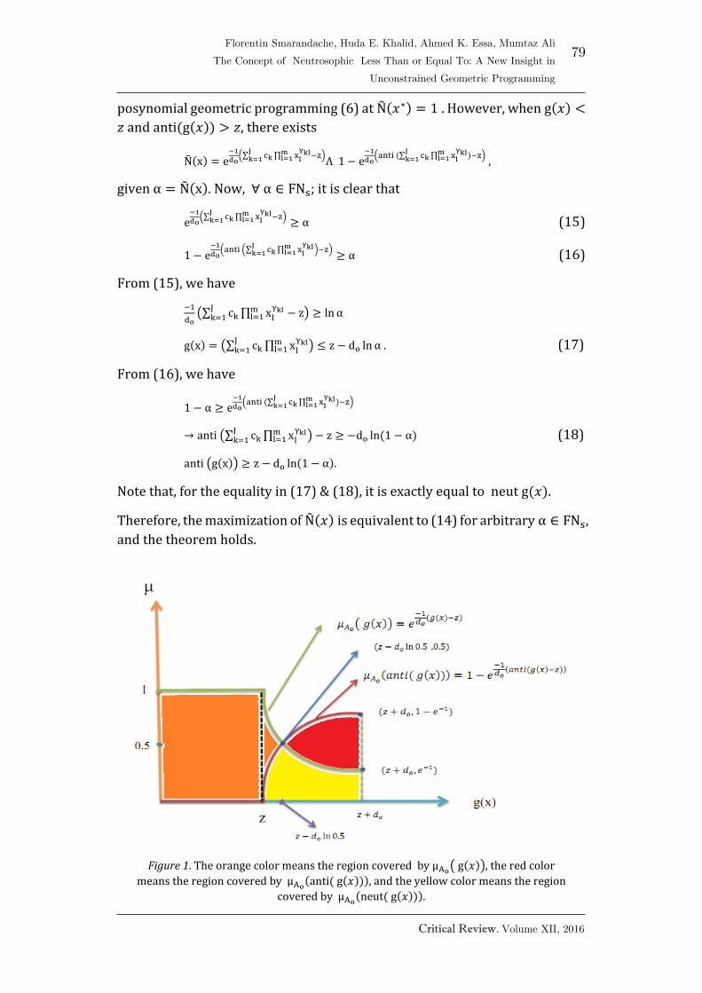
79
Critical Review. Volume XII, 2016
Florentin Smarandache, Huda E. Khalid, Ahmed K. Essa, Mumtaz Ali
The Concept of Neutrosophic Less Than or Equal To: A New Insight in
Unconstrained Geometric Programming
posynomial geometric programming (6) at Ñ(𝑥∗) = 1 . However, when g(𝑥) <
𝑧 and anti(g(𝑥)) > 𝑧, there exists
Ñ(x) = e−1
do(∑ ck
Jk=1
∏ xl
γklml=1 −z)
Ʌ 1 − e−1
do(anti (∑ ck
Jk=1
∏ xl
γklml=1 )−z)
,
given α = Ñ(x). Now, ∀ α ∈ FNs; it is clear that
e−1
do(∑ ck
Jk=1
∏ xl
γklml=1 −z)
≥ α (15)
1 − e−1
do(anti (∑ ck
Jk=1
∏ xl
γklml=1 )−z)
≥ α (16)
From (15), we have
−1
do(∑ ck
Jk=1 ∏ xl
γklml=1 − z) ≥ ln α
g(x) = (∑ ckJk=1 ∏ xl
γklml=1 ) ≤ z − do ln α . (17)
From (16), we have
1 − α ≥ e−1
do(anti (∑ ck
Jk=1
∏ xl
γklml=1 )−z)
→ anti (∑ ckJk=1 ∏ xl
γklml=1 ) − z ≥ −do ln(1 − α) (18)
anti (g(x)) ≥ z − do ln(1 − α).
Note that, for the equality in (17) & (18), it is exactly equal to neut g(𝑥).
Therefore, the maximization of Ñ(𝑥) is equivalent to (14) for arbitrary α ∈ FNs,
and the theorem holds.
Figure 1. The orange color means the region covered by μAo( g(𝑥)), the red color
means the region covered by μAo(anti( g(𝑥))), and the yellow color means the region
covered by μAo(neut( g(𝑥))).
80
Florentin Smarandache, Huda E. Khalid, Ahmed K. Essa, Mumtaz Ali
The Concept of Neutrosophic Less Than or Equal To: A New Insight in
Unconstrained Geometric Programming
Critical Review. Volume XII, 2016
4 Conclusion
The innovative concept and procedure explained in this article suit to the
neutrosophic GP. A neutrosophic less than or equal to form can be completely
turned into classical less than, greater than and equal forms. The feasible
region for unconstrained neutrosophic GP can be determined by a fuzzy
neutrosophic optimal point set in the fuzzy neutrosophic decision region
Ñ(x∗) .
5 References
[1] B.Y. Cao, Fuzzy Geometric Programming, Dordrecht: Springer Science
Business Media, 2002.
[2] B.Y. Cao & J. H. Yang, Advances in Fuzzy Geometric Programming, Berlin-
Heidelberg: Springer Verlag, 2007.
[3] D. Dubois, H. Prade, Fuzzy Sets and Systems. Theory and Applications,
New York: Academic Press, 1980.
[4] R. J. Duffin, E. L. Peterson, C. Zener. Geometric Programming. Theory and
Application, New York: John Wiley and Sons, 1967.
[5] V. Kandasamy & F. Smarandache, Fuzzy Relational Maps and
Neutrosophic Relational Maps, Rehoboth: American Research Press, 2004.
[6] H. E. Khalid, A. Y. Al-Bayati, Investigation in the Sensitivity Analysis of
Generalized Geometric Programming Problems, PhD Thesis, The Council of
the College of Computers Sciences and Mathematics University of Mosul,
2010.
[7] H. E. Khalid, An Original Notion to Find Maximal Solution in the Fuzzy
Neutrosophic Relation Equations (FNRE) with Geometric Programming (GP),
in “Neutrosophic Sets and Systems”, vol. 7, 2015, pp. 3-7.
[8] H. E. Khalid, The Novel Attempt for Finding Minimum Solution in Fuzzy
Neutrosophic Relational Geometric Programming (FNRGP) with (max , min )
Composition, in “Neutrosophic Sets and Systems”, vol. 11, 2016, pp. 107-112.
[9] F. Smarandache, Neutrosophic Overset, Neutrosophic Underset, and
Neutrosophic Offset. Similarly for Neutrosophic Over-/Under-/Off- Logic,
Probability, and Statistics, 168 p., Pons Editions, Bruxelles, Belgique, 2016,
https://arxiv.org/ftp/arxiv/papers/1607/1607.00234.pdf
81
Critical Review. Volume XII, 2016
Multi-Criteria Decision Making
Method for n-wise Criteria
Comparisons and Inconsistent
Problems
A. Elhassouny1, Florentin Smarandache2
1 Team RIITM, ENSIAS, University Mohammad V, Rabat, Morocco
2 Math & Science Department, University of New Mexico, Gallup, New Mexico, USA
Abstract
The purpose of this paper is to present an alternative of a hybrid method based on
Saaty’s Analytical Hierarchy Process and on the Technique for Order Preference by
using the Similarity to Ideal Solution method (AHP-TOPSIS) and, based on the AHP
and its use of pairwise comparisons, to extend it to a new method called α-D MCDM-
TOPSIS (α-Discounting Method for multi-criteria decision making-TOPSIS). The new
method overcomes the limits of AHP, which works only for pairwise comparisons of
criteria, to any-wise (n-wise) comparisons, with crisp coefficients or with interval-
valued coefficients. An extended MCMD method (called Extended α-D MCDM) of α-D
MCDM, introduced by Smarandache to solve decision making problems, is developed.
α-D MCDM-TOPSIS and Extended α-D MCDM are verified on several examples, to
demonstrate how they work with consistent, weak inconsistent or strong
inconsistent problems. Finally, we discuss and compare all methods.
Keyword
Decision making, Extended α-D MCDM, Consistency, Inconsistency, n-wise criteria
comparisons, AHP TOPSIS.
1 Introduction
Many economic, social or technological problems have been widely discussed
and resolved in recent years by multi-criteria decision making methods [8].
However, the quantity of data, the complexity of the modern world and the
recent technological advances have made obviously that MCDM methods are
more challenging than ever, hence the necessity of developing other methods,
able to give quality solutions.

82
A. Elhassouny, Florentin Smarandache
Multi-Criteria Decision Making Method for n-wise Criteria Comparisons
and Inconsistent Problems
Critical Review. Volume XII, 2016
Among MCDM methods, the most often used to improve the reliability of the
decision making process is the combined method AHP-TOPSIS [12], [3], [2],
[8], [10], [11] and [4].
AHP-TOPSIS is indeed a useful MCDM method to resolve difficult decision
making problems and to select the best of the alternatives. Its applications
are significant [8]: a support for management and planning of flight mission
at NASA [12]; a method to study how the traffic congestion of urban roads is
evaluated [3]; choosing logistics service provider in the mobile phone
industry domains [10]; summarizing an e-SCM performance for management
of supply chain [11]; evaluating faculty performance in engineering
education, or sharing capacity assessment knowledge of supply chain [4].
Our paper is organized as follows. In the next section (Section 2), a literature
survey for consistency problems is given. Section 3 and Section 4 focus on
AHP-TOPSIS, and on the proposed α-D MCDM-TOPSIS model, respectively.
The proposed method is tested on consistent, weak inconsistent and strong
inconsistent examples (in Section 5). AHP method employed to rank the
preferences is considered in Section 6. An extended α-D MCDM is introduced
in Section 7, and it is shown how it can be applied for ranking preferences.
We discuss developments via the use of an example to compare all methods.
Finally, we draw conclusions and envisage some perspectives.
2 Comparison of characteristics between AHP
and α-D MCDM: Consistency
2.1 A brief overview of Analytic Hierarchy Process (AHP)
AHP, introduced by the Saaty [6], is one of the most complete methods of
multi-criteria decision making technique, determining the weights of criteria
and ranking alternatives. The use of AHP only, or its hybrid use with other
methods, proved its capacity to solve MCDM problems and to be a popular
technique for determining weights — see more than a thousand references in
[9]. Besides the performance of AHP and its added value at both levels,
theoretical and practical, this method functions only if the problem is
perfectly consistent, which is rarely checked in real MCDM problems.
2.2 Description of α-D MCDM
α-D MCDM (α-Discounting Method for Multi-Criteria Decision Making) was
introduced by Smarandache — see [7]. The new method overcomes the limits
of AHP, which work only for pairwise comparisons of criteria, expanding to
any-wise (n-wise) comparisons.

83
Critical Review. Volume X, 2015
A. Elhassouny, Florentin Smarandache
Multi-Criteria Decision Making Method for n-wise Criteria Comparisons
and Inconsistent Problems
Smarandache used the homogeneous linear mathematical equations to
express the relationship between criteria with crisp coefficients or with
interval-valued coefficients also for non-linear equations, with crisp
coefficients or with interval-valued coefficients.
The two aims of α-D MCDM method were: firstly, to transform the equations
of each criterion with respect to other criteria that has only a null solution
into a linear homogeneous system having a non-null solution by multiplying
each criteria of the right hand by non-null positive parameters ;
secondly, to apply the “Fairness Principle” on the general solution of the
above system by discounting each parameter by the same value
( ).
2.2.1 α-D MCDM method
The general idea of the -D MCDM is to transform any MCDM inconsistent
problem (in which AHP does not work) to a MCDM consistent problem, by
discounting each coefficient by the same percentage.
Let us assume that 1 2= , , , nC C C C , with 2n , is a set of criteria, and let’s
construct a linear homogeneous system of equations.
Each criterion can be expressed as linear homogeneous equation, or as
non-linear equation, with crisp coefficients or with interval-valued
coefficients of other criteria —
.
Consequently, a comparisons matrix associated to this linear homogeneous
system is constructed.
To determine the weights of the criteria, we solve the previous system.
The α-D MCDM method is not designed to rank preferences iP based on iC
criteria, as AHP method does, but to determine only the weights of criteria in
any type of problems (consistent, inconsistent).
AHP as cited above is a complete method designed to calculate the weights of
criteria iC and to rank the preferences iP . In addition, when the AHP is used
with TOPSIS, or other MCDM method, we just benefit from the part of weight
calculation criteria and we use TOPSIS to rank preferences — or other MCDM
methods.
The same for α-D MCDM: firstly, it is just used to calculate the weight of
criteria, that will be used later by TOPSIS to rank preferences, and, secondly,

84
A. Elhassouny, Florentin Smarandache
Multi-Criteria Decision Making Method for n-wise Criteria Comparisons
and Inconsistent Problems
Critical Review. Volume XII, 2016
the α-D MCDM is extended to a complete method, in order to rank the
preferences.
Therefore, we use α-D MCDM for calculating the weight of criteria iC and not
to rank iP preferences.
We have —
= ({ }\ )i iC f C C .
Then, criteria iC is a linear equation of jC such as —
=1
=n
i ij j
j j i
C x C
.
So, the comparisons criteria matrix has the number of criteria by rows and
columns (rows number n = number of criteria, and columns number m =
number of equations). In the result, we have a square matrix ( ),
consequently we can calculate the determinant of this matrix. At this point,
we have an n n linear homogeneous system and its associated matrix —
1,1 1 1,2 2 1,
,1 1 ,2 2 ,
= 0
= 0
n n
n m n n n
x w x w x w
x w x w x w
1,1 1,
,1 ,
=
n
n n n
x x
X
x x
.
The difference between AHP and -D MCDM is the ability of the latter to work
with consistent and inconsistent problems, and if the problem is inconsistent,
-D MCDM method transforms it in a consistent problem, while AHP is
unable to do that, managing strictly consistent problems.
In the following, we deal with the relationship between determinant of
matrix and consistency, and the parameterization of system by in order to
get a consistent problem.
Property 1
— If ( ) = 0det X , the system has a solution (i.e. MCDM problem is consistent).
— If ( ) 0det X , the system has only the null solution (i.e. MCDM problem is
inconsistent).
85
Critical Review. Volume X, 2015
A. Elhassouny, Florentin Smarandache
Multi-Criteria Decision Making Method for n-wise Criteria Comparisons
and Inconsistent Problems
If the problem is inconsistent, then one constructs the parameterized matrix,
denoted , by parameterizing the right-hand in order to get
and use Fairness principe (set equal parameters to all criteria
). To get priority vector, one resolves the new
system obtained and set 1 to secondary variable, then normalize the vector
by dividing the sum of all components.
2.3 Consistency of decision making problems
In this section, we discuss the consistency of the MCDM problems for both
methods ( -D MCDM and AHP).
For resolving a linear system of equations, in mathematics we use raw
operations, such as substitution, interchange, … .
Definition 1 [7]
Applying any substitution raw operations on two equations, if it does not
influence the system consistency and there is an agreement of all equations,
we say that the linear system of equations (of the linear MCDM problem) is
consistent.
Definition 2 [7]
Applying any substitution raw operations on two equations, if equation result
is in disagreement with another, we say that the linear system of equations
(of the linear MCDM problem) is weakly consistent.
Definition 3 [7]
Applying any substitution raw operations on two equations, if equation result
is in opposition with another, we say that the linear system of equations (of
the linear MCDM problem) is strongly inconsistent.
2.4 Consistency
AHP provides the decision maker with a way of examining the consistency of
entries in a pairwise comparison matrix; the problem of accepting/rejecting
matrices has been largely discussed [5], [1], [13], especially regarding the
relation between the consistency and the scale used to represent the decision
maker’s judgments. AHP is too restrictive when the size of the matrix
increases, and when order n of judgment matrix is large; the satisfying
consistency is more difficult to be met [5], [1].

86
A. Elhassouny, Florentin Smarandache
Multi-Criteria Decision Making Method for n-wise Criteria Comparisons
and Inconsistent Problems
Critical Review. Volume XII, 2016
This problem may become a very difficult one when the decision maker is not
perfectly consistent, moreover, it seems impossible (AHP does not work)
when there are not pairwise comparisons, but all kind of comparisons
between criteria, such as n wise, because there is set a strict consistency
condition in the AHP, in order to keep the rationality of preference intensities
between compared elements.
In addition, the inconsistency exists in all judgments [5]; comparing three
alternatives — or more, it is possible that inconsistency exists when there are
more than 25 percent of the 3 3by reciprocal matrices with a consistency
ratio less than or equal to ten percent. Consequently, as the matrix size
increases, the percentage of inconsistency decreases dramatically [1], [5].
Furthermore, the AHP method sets a consistency ratio (CR) threshold
( ( ) > 0.1CR X ), which should not be exceeded, by examining the
inconsistency of the pairwise comparison matrix, but this requirement for
the Saaty’s matrix is not achievable in the real situations.
In order to overcome this deficiency, instead of the AHP we suggest
employing an α-D MCDM, which is very natural and more suitable for the
linguistic descriptions of the Saaty’s scale and, as a result of it, it is easier to
reach this requirement in the real situations.
Moreover, the attractiveness of -D MCDM is due to its potential to overcome
limits of AHP, which works only for pairwise comparisons of criteria,
expanding to n -wise (with 2n ) comparisons, with crisp coefficients or
with interval-valued coefficients. Therefore, α-D MCDM method works for
inconsistent, weak inconsistent and strong inconsistent problems.
As previously shown, in α-D MCDM method, in order to transform a
inconsistent MCDM problem to a consistent problem — we multiply each
criteria of the right hand by non-null positive parameters and
we use “Fairness Principle” assigning to each parameter the same value
( ).
Property 2
In α-D MCDM (and Fairness-Principle for coefficients ), the parameter (or
) signifies the degree of consistency and ( ) represents the
degree of inconsistency.
— If , then and represent the degree of consistency
and the degree of inconsistency, respectively, of the decision-making
problem.
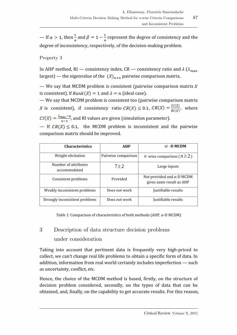
87
Critical Review. Volume X, 2015
A. Elhassouny, Florentin Smarandache
Multi-Criteria Decision Making Method for n-wise Criteria Comparisons
and Inconsistent Problems
— If , then and represent the degree of consistency and the
degree of inconsistency, respectively, of the decision-making problem.
Property 3
In AHP method, RI — consistency index, CR — consistency ratio and (
largest) — the eigenvalue of the pairwise comparison matrix.
— We say that MCDM problem is consistent (pairwise comparison matrix
is consistent), if and (ideal case).
— We say that MCDM problem is consistent too (pairwise comparison matrix
is consistent), if consistency ratio , , where
, and RI values are given (simulation parameter).
— If , the MCDM problem is inconsistent and the pairwise
comparison matrix should be improved.
Characteristics AHP -D MCDM
Weight elicitation Pairwise comparison n -wise comparison ( 2n )
Number of attributes
accommodated 7 2 Large inputs
Consistent problems Provided Not provided and α-D MCDM
gives same result as AHP
Weakly inconsistent problems Does not work Justifiable results
Strongly inconsistent problems Does not work Justifiable results
Table 1: Comparison of characteristics of both methods (AHP, α-D MCDM)
3 Description of data structure decision problems
under consideration
Taking into account that pertinent data is frequently very high-priced to
collect, we can’t change real life problems to obtain a specific form of data. In
addition, information from real world certainly includes imperfection — such
as uncertainty, conflict, etc.
Hence, the choice of the MCDM method is based, firstly, on the structure of
decision problem considered, secondly, on the types of data that can be
obtained, and, finally, on the capability to get accurate results. For this reason,

88
A. Elhassouny, Florentin Smarandache
Multi-Criteria Decision Making Method for n-wise Criteria Comparisons
and Inconsistent Problems
Critical Review. Volume XII, 2016
we detail the different types of all data structure decision problem, for
example:
— If decision matrix illustrates the importance of alternatives with respect of
criteria, the pairwise (or n -wise) comparison can’t be used directly in the
hybrid AHP-TOPSIS approach. Firstly, priority weights for criteria are
calculated using AHP technique, and then the alternatives are prioritized
using TOPSIS approach.
The derivation of weights is a central step in eliciting the decision-maker’s
preferences, but the hybrid AHP-TOPSIS method is more difficult to be met:
on one hand, AHP does not work in inconsistent problems, on the other hand
it cannot be employed for the n -wise comparisons criteria cases.
The problem can be abstracted as how to derive weights for a set of activities
according to their impact on the situation and the objective of decisions to be
made.
Hence, this study will extend AHP-TOPSIS to a MCDM to fit real world. A
complete and efficient procedure for decision making will then be provided.
The developed model has been analyzed to select the best alternative using
α-D MCDM and the technique for order preference by similarity to ideal
solution (TOPSIS) as a hybrid approach.
Let us assume that 1 2= , , , nC C C C is a set of Criteria, with 2n , and
1 2= , , , mA A A A is the set of Preferences (Alternatives), with 1m .
1
1,1 1, 1
,1 ,
n
n
n n n n
C C
x x C
x x C
1C 2C nC
1w 2w nw
1A 11a 12a 1na
2A 21a 22a 2na
mA 1ma 2ma mna
Table 2: Decision matrix
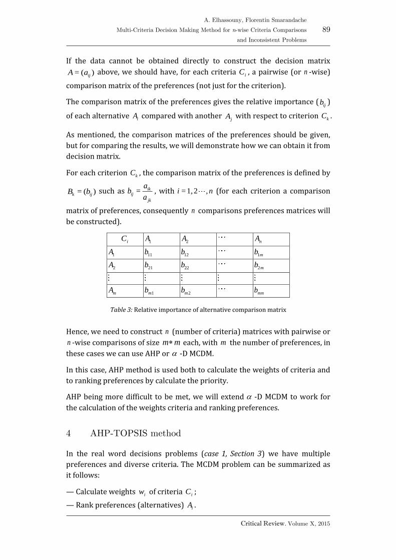
89
Critical Review. Volume X, 2015
A. Elhassouny, Florentin Smarandache
Multi-Criteria Decision Making Method for n-wise Criteria Comparisons
and Inconsistent Problems
If the data cannot be obtained directly to construct the decision matrix
= ( )ijA a above, we should have, for each criteria iC , a pairwise (or n -wise)
comparison matrix of the preferences (not just for the criterion).
The comparison matrix of the preferences gives the relative importance (ijb )
of each alternative iA compared with another jA with respect to criterion kC .
As mentioned, the comparison matrices of the preferences should be given,
but for comparing the results, we will demonstrate how we can obtain it from
decision matrix.
For each criterion kC , the comparison matrix of the preferences is defined by
= ( )k ijB b such as = ikij
jk
ab
a, with = 1,2 ,i n (for each criterion a comparison
matrix of preferences, consequently n comparisons preferences matrices will
be constructed).
iC 1A 2A nA
1A 11b 12b 1mb
2A 21b 22b 2mb
mA 1mb 2mb mmb
Table 3: Relative importance of alternative comparison matrix
Hence, we need to construct n (number of criteria) matrices with pairwise or
n -wise comparisons of size m m each, with m the number of preferences, in
these cases we can use AHP or -D MCDM.
In this case, AHP method is used both to calculate the weights of criteria and
to ranking preferences by calculate the priority.
AHP being more difficult to be met, we will extend -D MCDM to work for
the calculation of the weights criteria and ranking preferences.
4 AHP-TOPSIS method
In the real word decisions problems (case 1, Section 3) we have multiple
preferences and diverse criteria. The MCDM problem can be summarized as
it follows:
— Calculate weights iw of criteria iC ;
— Rank preferences (alternatives) iA .
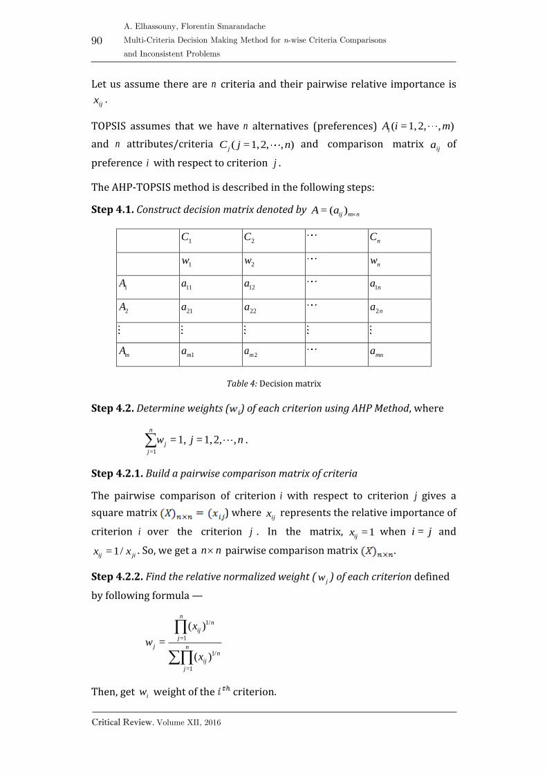
90
A. Elhassouny, Florentin Smarandache
Multi-Criteria Decision Making Method for n-wise Criteria Comparisons
and Inconsistent Problems
Critical Review. Volume XII, 2016
Let us assume there are n criteria and their pairwise relative importance is
ijx .
TOPSIS assumes that we have n alternatives (preferences) ( =1,2, , )iA i m
and n attributes/criteria ( =1,2, , )jC j n and comparison matrix ija of
preference i with respect to criterion j .
The AHP-TOPSIS method is described in the following steps:
Step 4.1. Construct decision matrix denoted by = ( )ij m nA a
1C 2C
nC
1w 2w
nw
1A 11a 12a 1na
2A 21a 22a 2na
mA 1ma 2ma mna
Table 4: Decision matrix
Step 4.2. Determine weights ( ) of each criterion using AHP Method, where
=1
=1, =1,2, ,n
j
j
w j n .
Step 4.2.1. Build a pairwise comparison matrix of criteria
The pairwise comparison of criterion i with respect to criterion j gives a
square matrix ) where ijx represents the relative importance of
criterion i over the criterion j . In the matrix, =1ijx when =i j and
=1/ij jix x . So, we get a n n pairwise comparison matrix .
Step 4.2.2. Find the relative normalized weight (jw ) of each criterion defined
by following formula —
1/
=1
1/
=1
( )
=
( )
nn
ij
j
j nn
ij
j
x
w
x
Then, get iw weight of the criterion.
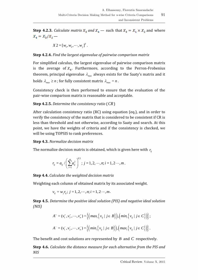
91
Critical Review. Volume X, 2015
A. Elhassouny, Florentin Smarandache
Multi-Criteria Decision Making Method for n-wise Criteria Comparisons
and Inconsistent Problems
Step 4.2.3. Calculate matrix and — such that and where
—
1 22 = [ , , , ]T
jX w w w .
Step 4.2.4. Find the largest eigenvalue of pairwise comparison matrix
For simplified calculus, the largest eigenvalue of pairwise comparison matrix
is the average of . Furthermore, according to the Perron-Frobenius
theorem, principal eigenvalue max always exists for the Saaty’s matrix and it
holds max n ; for fully consistent matrix =max n .
Consistency check is then performed to ensure that the evaluation of the
pair-wise comparison matrix is reasonable and acceptable.
Step 4.2.5. Determine the consistency ratio (CR )
After calculation consistency ratio (RC) using equation (eq.), and in order to
verify the consistency of the matrix that is considered to be consistent if CR is
less than threshold and not otherwise, according to Saaty and search. At this
point, we have the weights of criteria and if the consistency is checked, we
will be using TOPSIS to rank preferences.
Step 4.3. Normalize decision matrix
The normalize decision matrix is obtained, which is given here with ijr
0.5
2
=1
= / ; =1,2, , ; =1,2 ,m
ij ij ij
i
r a a j n i m .
Step 4.4. Calculate the weighted decision matrix
Weighting each column of obtained matrix by its associated weight.
= ; =1,2, , ; =1,2 ,ij j ijv w r j n i m .
Step 4.5. Determine the positive ideal solution (PIS) and negative ideal solution
(NIS)
1 2= ( , , , ) = | , |n i ij i ijA v v v max v j B min v j C ;
1 2= ( , , , ) = | , |n i ij i ijA v v v min v j B max v j C .
The benefit and cost solutions are represented by B and C respectively.
Step 4.6. Calculate the distance measure for each alternative from the PIS and
NIS

92
A. Elhassouny, Florentin Smarandache
Multi-Criteria Decision Making Method for n-wise Criteria Comparisons
and Inconsistent Problems
Critical Review. Volume XII, 2016
The distance measure for each alternative from the PIS is —
0.5
2
=1
= ( ) ; =1,2 ,n
i ij j
j
S v v i m
Also, the distance measure for each alternative from the NIS is —
0.5
2
=1
= ( ) ; =1,2 ,n
i ij j
j
S v v i m
Step 4.7. Determine the values of relative closeness measure
For each alternative we calculate the relative closeness measure as it follows:
= ; =1,2 ,( )
ii
i i
ST i m
S S
.
Rank alternatives set according to the order of relative closeness measure
values .
5 α-D MCDM-TOPSIS method
The MCDM problem description is the same as the one used in AHP-TOPSIS
method (Section 4), but in this case we have n -wise comparisons matrix of
criteria. Let us assume that 1 2= , , , nC C C C , with 2n , and 1 2, , , mA A A ,
with 1m , are a set of criteria and a set of preferences, respectively. Let us
assume that each criterion iC is a linear homogeneous equation of the other
criteria 1 2, , , nC C C :
= ({ }\ )i iC f C C .
The α-D MCDM-TOPSIS method is described in the following steps:
Step 5.1. Construct decision matrix denoted by = ( )ij m nA a
1C 2C
nC
1w 2w
nw
1A 11a 12a 1na
2A 21a 22a 2na
mA 1ma 2ma mna
Table 5: Decision matrix
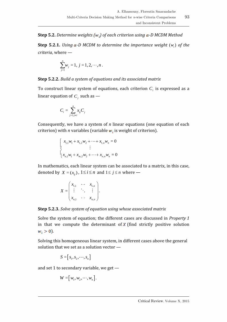
93
Critical Review. Volume X, 2015
A. Elhassouny, Florentin Smarandache
Multi-Criteria Decision Making Method for n-wise Criteria Comparisons
and Inconsistent Problems
Step 5.2. Determine weights ( ) of each criterion using -D MCDM Method
Step 5.2.1. Using -D MCDM to determine the importance weight ( )iw of the
criteria, where —
=1
=1, =1,2, ,n
j
j
w j n .
Step 5.2.2. Build a system of equations and its associated matrix
To construct linear system of equations, each criterion iC is expressed as a
linear equation of jC such as —
=1
=n
i ij j
j j i
C x C
Consequently, we have a system of n linear equations (one equation of each
criterion) with n variables (variable is weight of criterion).
1,1 1 1,2 2 1,
,1 1 ,2 2 ,
= 0
= 0
n n
n m n n n
x w x w x w
x w x w x w
In mathematics, each linear system can be associated to a matrix, in this case,
denoted by = ( )ijX x , 1 i n and 1 j n where —
1,1 1,
,1 ,
=
n
n n n
x x
X
x x
.
Step 5.2.3. Solve system of equation using whose associated matrix
Solve the system of equation; the different cases are discussed in Property 1
in that we compute the determinant of (find strictly positive solution
).
Solving this homogeneous linear system, in different cases above the general
solution that we set as a solution vector —
1 2= , , , nS s s s
and set 1 to secondary variable, we get —
1 2= , , , nW w w w .

94
A. Elhassouny, Florentin Smarandache
Multi-Criteria Decision Making Method for n-wise Criteria Comparisons
and Inconsistent Problems
Critical Review. Volume XII, 2016
Dividing each vector element on sum of all components of vector to get
normalized vector, where —
=1
= ; =1,2 ,j
j n
k
k
sw i n
s.
Step 5.2.4. Build a pairwise comparison matrix of criteria
The pairwise comparison of criterion i with respect to criterion j gives a
square matrix ) where ijx represents the relative importance of
criterion i over the criterion j . In the matrix, =1ijx when =i j and
=1/ij jix x . So we get a n n pairwise comparison matrix .
Step 5.2.5. Find the relative normalized weight (jw ) of each criterion defined
by the following formula —
1/
=1
1/
=1
( )
=
( )
nn
ij
j
j nn
ij
j
x
w
x
.
Then, get iw weight of the criterion.
Step 5.2.6. Calculate matrix and — such that and where
—
1 22 = [ , , , ]T
jX w w w .
Step 5.2.7. Find the largest eigenvalue of pairwise comparison matrix
For simplifying the calculus, the largest eigenvalue of pairwise comparison
matrix is the average of . Furthermore, according to the Perron-Frobenius
theorem, principal eigenvalue max always exists for the Saaty’s matrix and it
holds max n ; for fully consistent matrix =max n .
Consistency check is then performed to ensure that the evaluation of the
pair-wise comparison matrix is reasonable and acceptable.
Step 5.2.8. Determine the consistency ratio (CR )
After calculating consistency ratio (RC) using equation (eq.), and in order to
verify the consistency of the matrix that is considered to be consistent if CR is
less than threshold and not otherwise, according to Saaty and search.

95
Critical Review. Volume X, 2015
A. Elhassouny, Florentin Smarandache
Multi-Criteria Decision Making Method for n-wise Criteria Comparisons
and Inconsistent Problems
At this point, we have the weights of criteria and if the consistency is checked,
we will be using TOPSIS to rank preferences.
Step 5.3. Normalize decision matrix
The normalized decision matrix is obtained, which is given here with ijr
0.5
2
=1
= / ; =1,2, , ; =1,2 ,m
ij ij ij
i
r a a j n i m .
Step 5.4. Calculate the weighted decision matrix
Weighting each column of obtained matrix by its associated weight —
= ; =1,2, , ; =1,2 ,ij j ijv w r j n i m .
Step 5.5. Determine the positive ideal solution (PIS) and negative ideal solution
(NIS)
1 2= ( , , , ) = | , |n i ij i ijA v v v max v j B min v j C ;
1 2= ( , , , ) = | , |n i ij i ijA v v v min v j B max v j C .
The benefit and cost solutions are represented by B and C , respectively.
Step 5.6. Calculate the distance measure for each alternative from the PIS and
NIS
The distance measure for each alternative from the PIS is —
0.5
2
=1
= ( ) ; =1,2 ,n
i ij j
j
S v v i m
.
Also, the distance measure for each alternative from the NIS is —
0.5
2
=1
= ( ) ; =1,2 ,n
i ij j
j
S v v i m
.
Step 5.7. Determine the values of relative closeness measure
For each alternative, we calculate the relative closeness measure as it
follows:
= ; =1,2 ,( )
ii
i i
ST i m
S S
.
Rank alternatives set according to the order of relative closeness measure
values .

96
A. Elhassouny, Florentin Smarandache
Multi-Criteria Decision Making Method for n-wise Criteria Comparisons
and Inconsistent Problems
Critical Review. Volume XII, 2016
6 Numerical examples
We examine a numerical example in which a synthetic evaluation desire to
rank four alternatives 1A , 2A , 3A and 4A with respect to three benefit
attribute 1C , 2C and 3C .
1C 2C 3C
1w 2w 3w
1A 7 9 9
2A 8 7 8
3A 9 6 8
4A 6 7 8
Table 6: Decision matrix
In the examples below, we use α-D MCDM and AHP (if it works) to calculate
the weights of the criteria 1w , 2w and 3w . After we used TOPSIS to rank the
four alternatives, the decision matrix (Table 6) is used for the three following
examples.
6.1 Consistent Example 1
We use the -D MCDM. Let the Set of Criteria be 1 2 3, ,C C C with
and .
Let us consider the system of equations associated to MCDM problem and its
associated matrix.
4
3
12
x y
y z
xz
1 4 0
1 = 0 1 3
10 1
12
X
.
We calculate (in this case, equal = 0); then MCDM problem is
consistent; we solve the system; we get the following solution —
= 12 3S z z z .
Setting 1 to secondary variable, the general solution becomes —
= 12 3 1S ,
and normalizing the vector (dividing by sum=12+3+1), the weights vector is:

97
Critical Review. Volume X, 2015
A. Elhassouny, Florentin Smarandache
Multi-Criteria Decision Making Method for n-wise Criteria Comparisons
and Inconsistent Problems
12 3 1=
16 16 16W
.
Using AHP, we get the same result.
The pairwise comparison matrix of criteria is:
1 4 12
11= 1 3
4
1 11
12 3
X
,
whose maximum eigenvalue is = 3max and its corresponding normalized
eigenvector (Perron-Frobenius vector) is —
12 3 1=
16 16 16W
.
We use TOPSIS to rank the four alternatives.
2
ija 1C 2C 3C
iw 12/16 3/16 1/16
1A 49 81 81
2A 64 49 64
3A 81 36 64
4A 36 49 64
2
=1
n
ijia
230 215 273
Table 7: Calculate 2( )ija for each column
ijr
1C 2C 3C
iw 12/16 3/16 1/16
1A 0.4616 0.6138 0.5447
2A 0.5275 0.4774 0.4842
3A 0.5934 0.4092 0.4842
4A 0.3956 0.4774 0.4842
2
=1
n
ijia 230 215 273
Table 8: Divide each column by 2 1/2
=1( )
n
ijia to get
ijr

98
A. Elhassouny, Florentin Smarandache
Multi-Criteria Decision Making Method for n-wise Criteria Comparisons
and Inconsistent Problems
Critical Review. Volume XII, 2016
ijv
1C 2C 3C
iw 12/16 3/16 1/16
1A 0.3462 0.1151 0.0340
2A 0.3956 0.0895 0.0303
3A 0.4451 0.0767 0.0303
4A 0.2967 0.0895 0.0303
maxv 0.4451 0.1151 0.0340
minv 0.2967 0.0767 0.0303
Table 9: Multiply each column by jw to get
ijv
Alternative iS
iS iT Rank
1A 0.0989 0.0627 0.3880 3
2A 0.0558 0.0997 0.6412 2
3A 0.0385 0.1484 0.7938 1
4A 0.1506 0.0128 0.0783 4
Table 10: The separation measure values and the final rankings
for decision matrix (Table 4) using AHP-TOPSIS and α-D MCDM-TOPSIS
Table 10 presents the rank of alternatives ( 1A , 2A , 3A , 4A ) and separation
measure values of each alternative from the PIS and from NIS in which the
weighted values are calculated by AHP or α-D MCDM. Both methods, AHP and
α-D MCDM with Fairness Principle, give the same weights as proven above
methods together give same result in consistent problem.
6.2 Weak inconsistent Example 2 where AHP does not work
Let us consider another example investigated by [7] for which AHP does not
work (i.e. AHP-TOPSIS does not work too); we use the α-D MCDM to calculate
the weights values and ranking the four alternatives by TOPSIS (see Table 14).
Let the Set of Criteria be 1 2 3, ,C C C with and
. Let us consider the system of equations associated to MCDM
problem and its associated matrix.
2 3
2
3
x y z
xy
xz

99
Critical Review. Volume X, 2015
A. Elhassouny, Florentin Smarandache
Multi-Criteria Decision Making Method for n-wise Criteria Comparisons
and Inconsistent Problems
1 2 3
11= 1 0
2
10 1
3
X
.
The solution of this system is ; be the sum of weights = 1, then
this solution is not acceptable.
Parameterizing the right-hand side coefficient of each equation by we get:
We solve the system and we get the following solution —
or 3 4=2 3
x xS x
.
Setting 1 to secondary variable, the general solution becomes —
3 4= 12 3
S
.
Applying Fairness Principle, then replacing 1 2 3 4= = = = , whence
2=
2 .
2 2= 1
4 6S
.
Normalizing vector (dividing by sum), the weights vector is:
= 0.62923 0.22246 0.14831W .
TOPSIS is used to rank the four alternative: application of TOPSIS method is in
the same manner as in the previous example (the four alternatives ( Ai ) are
ranked in the following Table 14).

100
A. Elhassouny, Florentin Smarandache
Multi-Criteria Decision Making Method for n-wise Criteria Comparisons
and Inconsistent Problems
Critical Review. Volume XII, 2016
2
ija 1C 2C 3C
0.62923 0.22246 0.14831
1A 49 81 81
2A 64 49 64
3A 81 36 64
4A 36 49 64
2
=1
n
ijia
230 215 273
Table 11: Calculate 2( )ija for each column
ijr
1C 2C 3C
0.62923 0.22246 0.14831
1A 0.4616 0.6138 0.5447
2A 0.5275 0.4774 0.4842
3A 0.5934 0.4092 0.4842
4A 0.3956 0.4774 0.4842
2
=1
n
ijia
230 215 273
Table 12: Divide each column by 2 1/2
=1( )
n
ijia to get
ijr
ijv
1C 2C 3C
0.62923 0.22246 0.14831
1A 0.2904 0.1365 0.0808
2A 0.3319 0.1062 0.0718
3A 0.3734 0.0910 0.0718
4A 0.2489 0.1062 0.0718
maxv 0.3734 0.1365 0.0808
minv 0.2489 0.0910 0.0718
Table 13: Multiply each column by jw to get
ijv
Alternative
iS iS iT Rank
1A 0.0830 0.0622 0.4286 3
2A 0.0522 0.0844 0.6178 2
3A 0.0464 0.1245 0.7285 1
4A 0.1284 0.0152 0.1057 4
Table 14: The separation measure values and the final rankings
for decision matrix (Table 4) using -D MCDM-TOPSIS
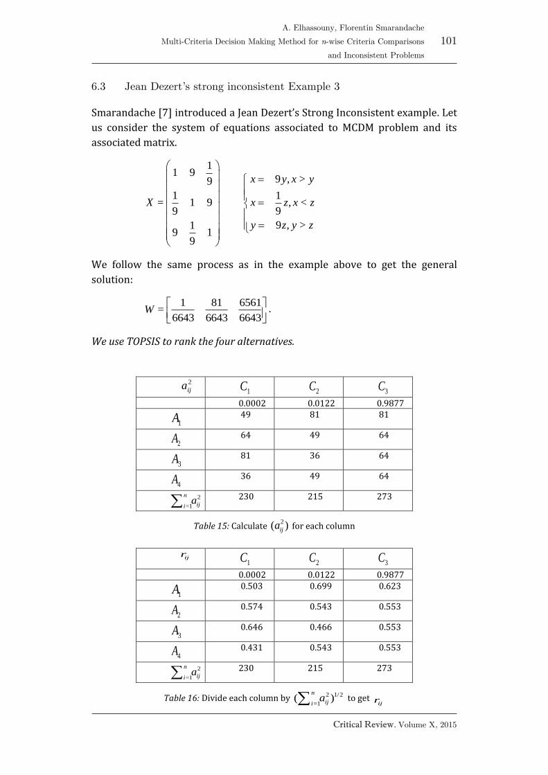
101
Critical Review. Volume X, 2015
A. Elhassouny, Florentin Smarandache
Multi-Criteria Decision Making Method for n-wise Criteria Comparisons
and Inconsistent Problems
6.3 Jean Dezert’s strong inconsistent Example 3
Smarandache [7] introduced a Jean Dezert’s Strong Inconsistent example. Let
us consider the system of equations associated to MCDM problem and its
associated matrix.
11 9
9
1= 1 9
9
19 1
9
X
9 , >
1, <
9
9 , >
x y x y
x z x z
y z y z
We follow the same process as in the example above to get the general
solution:
1 81 6561=
6643 6643 6643W
.
We use TOPSIS to rank the four alternatives.
2
ija 1C 2C 3C
0.0002 0.0122 0.9877
1A 49 81 81
2A 64 49 64
3A 81 36 64
4A 36 49 64
2
=1
n
ijia 230 215 273
Table 15: Calculate 2( )ija for each column
ijr
1C 2C 3C
0.0002 0.0122 0.9877
1A 0.503 0.699 0.623
2A 0.574 0.543 0.553
3A 0.646 0.466 0.553
4A 0.431 0.543 0.553
2
=1
n
ijia 230 215 273
Table 16: Divide each column by 2 1/2
=1( )
n
ijia to get
ijr

102
A. Elhassouny, Florentin Smarandache
Multi-Criteria Decision Making Method for n-wise Criteria Comparisons
and Inconsistent Problems
Critical Review. Volume XII, 2016
ijv
1C 2C 3C
0.0002 0.0122 0.9877
1A 0.0001 0.0075 0.5380
2A 0.0001 0.0058 0.4782
3A 0.0001 0.0050 0.4782
4A 0.0001 0.0058 0.4782
maxv 0.0001 0.0075 0.5380
minv 0.0001 0.0050 0.4782
Table 17: Multiply each column by jw to get
ijv
Alternative
iS iS
iT Rank
1A 0.0000 0.0598
0.999668 1
1A 0.0598 0.0008
0.013719 2
1A 0.0598 0.0000
0.000497 4
1A 0.0598 0.0008
0.013715 3
Table 18: The separation measure values and the final rankings
for decision matrix (Table 4) using α-D MCDM-TOPSIS
7 AHP method
As we proved in Section 3. Description of data structure decision problems
under consideration, AHP method can be used in the second case, in which
data is structured as pairwise comparisons of matrices of preferences.
Let us assume that X is the comparison matrix of criteria; for each criterion
kC ( = 1,2, ,k n ) we have a comparison matrix of preferences kB and the
consistency condition is perfect.
We use AHP to determine the importance weight ( )iw of the criteria.
We apply again AHP method for each comparison matrices of preferences kB
to determine the maximum eigenvalue and its associate eigenvector (same
that is used to determine the weights of criteria).
For each matrix kB (associated to kC ), we calculate the max and priority
vector (eigenvector).

103
Critical Review. Volume X, 2015
A. Elhassouny, Florentin Smarandache
Multi-Criteria Decision Making Method for n-wise Criteria Comparisons
and Inconsistent Problems
iC 1A 2A
nA Priority vector
1A 11a 12a
1ma 1ip
2A 21a 22a
2ma 2ip
mA 1ma 2ma
mma mip
Table 19: Comparison matrix of the preferences with priority vector in latest column
We get a decision matrix (different from the decision matrix above), formed
using priority vectors, in which the entries of the decision matrix are ijp , and
not ija .
1w 2w
nw
11p 12p
1np
21p 22p
2np
1mp 2mp
mnp
Table 20: Decision matrix of priority of preferences
The last step of AHP method is to rank the preferences using the following
formula —
=1
n
j ij
j
w p .
1w 2w
nw
11p 12p
1np 1=1
n
j jjw p
21p 22p
2np 2=1
n
j jjw p
1mp 2mp
mnp =1
n
j mjjw p
Table 21: Ranking decision matrix
7.1 Numerical examples
Let us consider the three numerical examples (Section 6) and the decision
matrix mentioned above.

104
A. Elhassouny, Florentin Smarandache
Multi-Criteria Decision Making Method for n-wise Criteria Comparisons
and Inconsistent Problems
Critical Review. Volume XII, 2016
For weak inconsistent and strong inconsistent examples, AHP does not work,
as proved above, consequently the AHP method will be applied on consistent
example 1.
The weights of criteria are calculated by using AHP (consistent example 1,
Section 6).
As mentioned above (case 2, Section 3), for applying AHP we need to
construct three pairwise comparisons matrices of size 4 4 each.
1 7/8 7/9 7/6
8/7 1 8/9 8/6
9/7 7/8 1 9/6
6/7 7/8 6/9 1
1 9/7 9/6 9/7
7/9 1 7/6 1
6/9 6/7 1 6/7
7/9 1 7/6 1
1 9/8 9/8 9/8
8/9 1 1 1
8/9 1 1 1
8/9 1 1 1
Table 22: Relative importance comparison matrix of alternatives for each criteria
We apply AHP method on three pairwise comparison matrices to rank the
preferences, and calculate priority (i.e., normalized eigenvector), consistency
index (CI) and consistency ratio (CR) for each matrix.
The eigenvalue, consistency index (CI) and consistency ratio (CR) for each
matrix are: C1 — (CR =0, CI=0, λ = 4), C2 — (CR =0, CI=0, λ = 4) and C3 — (CR
=0, CI=0, λ = 4).
The priority vectors for three matrices are listed respectively in Table 23.
Priority vector
1 7/8 7/9 7/6 0.2333
8/7 1 8/9 8/6 0.2667
9/7 7/8 1 9/6 0.3000
6/7 7/8 6/9 1 0.2000
Priority vector
1 9/7 9/6 9/7 0.3103

105
Critical Review. Volume X, 2015
A. Elhassouny, Florentin Smarandache
Multi-Criteria Decision Making Method for n-wise Criteria Comparisons
and Inconsistent Problems
7/9 1 7/6 1 0.2414
6/9 6/7 1 6/7 0.2069
7/9 1 7/6 1 0.2414
Priority vector
1 9/8 9/8 9/8 0.2727
8/9 1 1 1 0.2424
8/9 1 1 1 0.2424
8/9 1 1 1 0.2424
Table 23: Relative importance comparison matrix of alternatives for each criteria
The last step of AHP method is applying it to rank the preferences using the
following formula (resulted as listed in the last column of the
matrix above).
Rank
12/16 3/16 1/16
0.2333 0.3103 0.2727 0.2502 3
0.2667 0.2414 0.2424 0.2604 2
0.3000 0.2069 0.2424 0.2789 1
0.2000 0.2414 0.2424 0.2104 4
Table 24: Decision matrix of priority of preferences and its ranking
8 Extended α-D MCDM
α-D MCDM introduced by Smarandache is not designed to rank preferences,
but only for generating the weights for preferences or criteria, based on their
-wise matrix comparison. Hence, we proposed above a new method, called
α-D MCDM-TOPSIS, employed to calculate the criteria weights for pairwise
comparison matrices and for -wise comparison matrices of criteria, in which
α-D MCDM is used for calculate criteria weights, and TOPSIS — to rank the
preferences.
In this section, we do not focus on criteria weights problem of -D MCDM, as
discussed above and calculated for the three examples, but we propose an
extension of α-D MCDM benefiting the skills of α-D MCDM to calculate
maximum eigenvalue and its associate eigenvector of -wise comparison
matrix, in order to apply it again on -wise matrices of preferences.
An extended -D MCDM can be described as it follows:

106
A. Elhassouny, Florentin Smarandache
Multi-Criteria Decision Making Method for n-wise Criteria Comparisons
and Inconsistent Problems
Critical Review. Volume XII, 2016
Let us consider the second case of data structure decision problem (Section
3) — for each criterion corresponds a pairwise (or n-wise) comparison
matrix of preferences and criteria.
Step 8.1 We use -D MCDM to calculate the weight ( ) of the criteria
Step 8.2 We apply again α-D MCDM method for each comparison matrices of
preferences to determine the maximum eigenvalue and its associate
eigenvector (the same that is used to determine the weights of criteria).
For each matrix (associated to ), we calculate the and priority
vector (eigenvector).
We get —
iC 1A 2A
nA Priority vector
1A 11a 12a
1ma 1ip
2A 21a 22a
2ma 2ip
mA 1ma 2ma
mma mip
Table 25: Comparison matrix of the preferences with priority vector in latest column
Step 8.3 We get a decision matrix (different from the decision matrix above),
formed using priority vectors, in which the entries of the decision matrix are
, and not .
1w 2w
nw
11p 12p
1np
21p 22p
2np
1mp 2mp
mnp
Table 26: Decision matrix of priority of preferences
Step 8.4 We employ the following formula (simple additive weighting) to rank
the preferences —
=1
n
j ij
j
w p .

107
Critical Review. Volume X, 2015
A. Elhassouny, Florentin Smarandache
Multi-Criteria Decision Making Method for n-wise Criteria Comparisons
and Inconsistent Problems
1w 2w
nw
11p 12p
1np 1=1
n
j jjw p
21p 22p
2np 2=1
n
j jjw p
1mp 2mp
mnp =1
n
j mjjw p
Table 27: Ranking decision matrix
8.1 Numerical examples
Let us consider the three examples mentioned above (numerical consistent,
weak inconsistent and strong inconsistent examples (Section 6).
We do not repeat the calculation of weights criteria by using α-D MCDM,
because it was already done in Section 6, and we got the following priority
vectors of criteria:
Consistent example 1 —
12 3 1=
16 16 16W
.
Weak inconsistent example 2 —
= 0.62923 0.22246 0.14831W .
Strong inconsistent example 3 —
1 81 6561=
6643 6643 6643W
.
We construct three comparisons matrices of size 4 4 each (or three linear
homogeneous systems), based on decision matrix of Section 6, and apply
extended α-D MCDM to the three examples.
Let
1( ) =m A x , 2( ) =m A y , 3( ) =m A z and 4( ) =m A t .
For criteria 1C —
• 2A is 8 seventh as important as 1A ,

108
A. Elhassouny, Florentin Smarandache
Multi-Criteria Decision Making Method for n-wise Criteria Comparisons
and Inconsistent Problems
Critical Review. Volume XII, 2016
• 3A is 9 seventh as important as 1A ,
• 4A is 6 seventh as important as 1A .
The linear homogeneous system associated is —
8
7
9
7
6
7
y x
z x
t x
and its general solution is —
7 8 9 6=
30 30 30 30W
.
For criteria 2C —
• 1A is 9 sixth as important as 3A ,
• 3A is 7 sixth as important as 3A ,
• 4A is 7 sixth as important as 3A .
The linear homogeneous system associated is —
9
6
7
6
7
6
x z
y z
t z
and its general solution is —
9 7 6 7=
29 29 29 29W
.
For criteria 3C —
• 1A is 9 eighth as important as 2A ,
• 2A , 3A and 4A have the same importance.

109
Critical Review. Volume X, 2015
A. Elhassouny, Florentin Smarandache
Multi-Criteria Decision Making Method for n-wise Criteria Comparisons
and Inconsistent Problems
The associated linear homogeneous system is —
9
8x y
y z
t z
and its general solution is —
9 8 8 8=
33 33 33 33W
.
The results of extended α-D MCDM are summarized in the Table 24:
Consistent example 1 —
Rank
12/16 3/16 1/16
7/30 9/29 9/33 0.2502 3
8/30 7/29 8/33 0.2604 2
9/30 6/29 8/33 0.2789 1
6/30 7/29 8/33 0.2104 4
Weak inconsistent example 2 —
Rank
0.62923 0.22246 0.14831
7/30 9/29 9/33 0.2563 3
8/30 7/29 8/33 0.2574 2
9/30 6/29 8/33 0.2707 1
6/30 7/29 8/33 0.2155 4
Strong inconsistent example 3 —
Rank
1/6643 81/6643 6561/6643
7/30 9/29 9/33 0.27318 1
8/30 7/29 8/33 0.24242 2
9/30 6/29 8/33 0.24200 4
6/30 7/29 8/33 0.24241 3
Table 24: Decision matrix of priority of preferences and its ranking using Extended -DMCDM
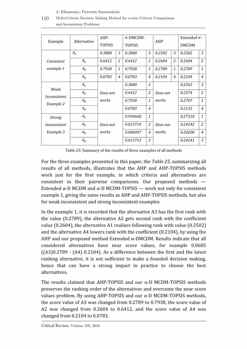
110
A. Elhassouny, Florentin Smarandache
Multi-Criteria Decision Making Method for n-wise Criteria Comparisons
and Inconsistent Problems
Critical Review. Volume XII, 2016
Example Alternative AHP-
TOPSIS
-DMCDM-
TOPSIS AHP
Extended -
DMCDM
Consistent
example 1
0.3880 3 0.3880 3 0.2502 3 0.2502 3
0.6412 2 0.6412 2 0.2604 2 0.2604 2
0.7938 1 0.7938 1 0.2789 1 0.2789 1
0.0783 4 0.0783 4 0.2104 4 0.2104 4
Weak
Inconsistent
Example 2
Does not
works
0.3880 3
Does not
works
0.2563 3
0.6412 2 0.2574 2
0.7938 1 0.2707 1
0.0783 4 0.2155 4
Strong
Inconsistent
Example 3
Does not
works
0.999668 1
Does not
works
0.27318 1
0.013719 2 0.24242 2
0.000497 4 0.24200 4
0.013715 3 0.24241 3
Table 25: Summary of the results of three examples of all methods
For the three examples presented in this paper, the Table 25, summarizing all
results of all methods, illustrates that the AHP and AHP-TOPSIS methods
work just for the first example, in which criteria and alternatives are
consistent in their pairwise comparisons. Our proposed methods —
Extended α-D MCDM and α-D MCDM-TOPSIS — work not only for consistent
example 1, giving the same results as AHP and AHP-TOPSIS methods, but also
for weak inconsistent and strong inconsistent examples.
In the example 1, it is recorded that the alternative A3 has the first rank with
the value (0.2789), the alternative A2 gets second rank with the coefficient
value (0.2604), the alternative A1 realizes following rank with value (0.2502)
and the alternative A4 lowers rank with the coefficient (0.2104), by using the
AHP and our proposed method Extended α-DMCDM. Results indicate that all
considered alternatives have near score values, for example 0.0685
((A3)0.2789 - (A4) 0.2104). As a difference between the first and the latest
ranking alternative, it is not sufficient to make a founded decision making,
hence that can have a strong impact in practice to choose the best
alternatives.
The results claimed that AHP-TOPSIS and our α-D MCDM-TOPSIS methods
preserves the ranking order of the alternatives and overcome the near score
values problem. By using AHP-TOPSIS and our α-D MCDM-TOPSIS methods,
the score value of A3 was changed from 0.2789 to 0.7938, the score value of
A2 was changed from 0.2604 to 0.6412, and the score value of A4 was
changed from 0.2104 to 0.0783.

111
Critical Review. Volume X, 2015
A. Elhassouny, Florentin Smarandache
Multi-Criteria Decision Making Method for n-wise Criteria Comparisons
and Inconsistent Problems
The bigger differences between the score values of alternatives 0.7155 ((A3)
0.7938 - (A4) 0.0783) is also subject to gain additional insights.
In the two last examples (weak inconsistent and strong inconsistent), one
sees that the importance of discounting in our approaches suggest that they
can be used to solve real-life problems in which criteria are not only pairwise,
but n-wise comparisons, and the problems are not perfectly consistent. It is
however worth to note that the ranking order of the four alternatives
obtained by both methods is similar, but score values are slightly different.
Both Extended α-D MCDM and α-D MCDM-TOPSIS methods allow taking into
consideration any numbers of alternatives and any weights of criteria.
9 Conclusions
We have proposed two multi-criteria decision making methods, Extended α-
D MCDM and α-D MCDM-TOPSIS models that allow to work for consistent
and inconsistent MCDM problems. In addition, three examples have
demonstrated that the α-D MCDM-TOPSIS model is efficient and robust.
Our approaches, Extended α-D MCDM and α-D MCDM-TOPSIS, give the same
result as AHP-TOPSIS and AHP in consistent MCDM problems and elements
of decision matrix are pairwise comparisons, but for weak inconsistent and
strong inconsistent MCDM problems in which AHP and AHP-TOPSIS are
limited and unable, our proposed methods — Extended α-D MCDM and α-D
MCDM-TOPSIS — give justifiable results.
Furthermore, our proposed approaches — α-D MCDM-TOPSIS and Extended
α-D MCDM — can be used to solve real-life problems in which criteria are not
only pairwise, but n-wise comparisons, and the problems are not perfectly
consistent.
References
[1] Alonso, J.A., Lamata, M. Consistency in the analytic hierarchy process: a
new approach. In “International Journal of Uncertainty, Fuzziness and
Knowledge-Based Systems” 14 (4), 445–459, 2006.
[2] Ghosh, D.N. Analytic hierarchy process and TOPSIS method to evaluate
faculty performance in engineering education. Dipendra Nath Ghosh et al.,
UNIASCIT 1 (2), 63–70, 2011.
[3] Jayanta, A., Guptaa, P., Gargb, S.K., Khana, M. TOPSIS-AHP based
approach for selection of reverse logistics service provider: A case study of
mobile phone industry. Procedia Engineering 97, Elsevier 97, 2147–2156,
2014. DOI: 10.1016/j.proeng.2014.12.458.
112
A. Elhassouny, Florentin Smarandache
Multi-Criteria Decision Making Method for n-wise Criteria Comparisons
and Inconsistent Problems
Critical Review. Volume XII, 2016
[4] Maheshwarkar, M., Sohani, N. Combined AHP-TOPSIS based approach
for the evaluation of knowledge sharing capabilities of supply chain partners.
Management Science and Engineering 7(3), 27–32, 2013. DOI:
10.3968/j.mse.1913035X20130703.2573.
[5] Pelaez, J.I., Lamata, M.T. New measure of consistency for positive
reciprocal matrices. In “International Journal Computers and Mathematics
with Applications”, Elsevier 46, 1839–1845, 2003. DOI: lO.l016/SO898-
1221(03) 00407-3.
[6] Saaty, T. Fundamentals of decision making and priority theory with the
AHP. RWS Publications, Pittsburgh, PA, U.S.A., 1994.
[7] Smarandache, F.: α-discounting method for multi-criteria decision
making (α-D MCDM). Fusion 2010 International Conference, Scotland,
2010; http://fs.gallup.unm.edu/alpha-DiscountingMCDM-book.pdf
[8] Tavana, M., Hatami-Marbini, A. A group AHP-TOPSIS framework for
human spaceflight mission planning at NASA. In “Expert Systems with
Applications” 38, 13, 588–13,603, 2011. DOI: 10.1016/j.eswa.2011.04. 108.
[9] Triantaphyllou, E., Mann, S.H. Using the analytic hierarchy process for
decision making in engineering application: dome challenges. In
“International Journal of Industrial Engineering: Applications and
Practice” 2 (1), 35–44, 1995.
[10] Tyagia, M., Kumarb, P., Kumarc, D. A hybrid approach using AHP-
TOPSIS for analyzing e-SCM performance. 12th Global Congress On
Manufac-turing and Management Engineering, Elsevier 97, 2195–2203,
2014.
[11] Wu, M. TOPSIS-AHP simulation model and its application to supply
chain management. In “World Journal of Modelling and Simulation”, 3 (3),
196–201, 2007.
[12] Yu, J., Wang, L., Gong, X. Study on the status evaluation of urban road
intersections traffic congestion based on AHP-TOPSIS model. 13th COTA
International Conference of Transportation Professionals, CICTP 2013 96,
609–616, 2013.
[13] Weak consistency: A new approach to consistency in the Saaty’s
analytic hierarchy process. In “Mathematica”, 52 (2), 71–83.

Critical Review A Publication of Society for Mathematics of Uncertainty
Publisher: Volume XII, 2016 Center for Mathematics of Uncertainty
Creighton University
Contributors to current issue: Mumtaz Ali, Assia Bakali, Said Broumi, A. Elhassouny,
Ahmed K. Essa, Huda E. Khalid, A. A. Salama, Florentin Smarandache, Mohamed
Talea.
Papers in current issue: Interval Valued Neutrosophic Graphs; Neutrosophic Crisp
Probability Theory & Decision Making Process; On Strong Interval Valued
Neutrosophic Graphs; The Concept of Neutrosophic Less than or Equal: A New Insight
in Unconstrained Geometric Programming; Multi-Criteria Decision Making Method for
n-wise Criteria Comparisons and Inconsistent Problems.