issn 1980-9743 soils and rocks an nternational journal of ...numerical modeling of unsaturated soils...
TRANSCRIPT

Volume , NJanuary-April 2016
39 . 1
Soils and RocksAn International Journal of Geotechnical
and Geoenvironmental Engineering
SOILS and ROCKS An nternational Journal of Geotechnical and Geoenvironmental EngineeringI
Volume , N. 1, January-April 201639
Table of Contents
Soils and R
ocks Volume 39, N
. 1 2016
ISSN 980-97431
BMS
ARTICLES
State Variables in Saturated-Unsaturated Soil Mechanics
Numerical and Experimental Analysis of Horizontal Stress Changes and Soil Collapse DuringChemical Dissolution in a Modified Oedometer Cell
Alternative Method for Analysing Hydromechanical Behaviour of Unsaturated Soils
Recent Developments and Limitations of the SFG Model
Effectiveness of Capillary Barrier and Vegetative Slope Covers in Maintaining Soil Suction
Influence of Poisson’s Ratio on the Stress vs. Settlement Behavior of Shallow Foundations inUnsaturated Fine-Grained Soils
Statistical Assessment of Hydraulic Properties of Unsaturated Soils
Numerical Modeling of Unsaturated Soils Problems
D.G. Fredlund 3
C. Lins, N. Silva, L. Guimarães, A. Lima, I. Gomes 19
M.M.A. Mascarenha, M.P. Cordão Neto, M.T.M.G. Silva 29
D. Sheng 41
H. Rahardjo, S. Krisnanto, E.C. Leong 51
W.T. Oh, S.K. Vanapalli 71
G.F.N. Gitirana Jr., D.G. Fredlund 81
M.D. Fredlund 97
Special Issue: Unsaturated SoilsGuest editors:
G.F.N. Gitirana Jr. & D.G. Fredlund
0
5
25
75
95
100
0
5
25
75
95
100
0
5
25
75
95
100
0
5
25
75
95
100

Issue Date: April 2016
Issue: 400 copies and 800 online-distributed copies
Manuscript Submission: For review criteria and manuscript submission information, see Instructions for Authors at the end.
Disclaimer: The opinions and statements published in this journal are solely the author’s and not necessarily reflect the views or opinionsof the publishers (ABMS and SPG). The publishers do not accept any liability arising in any way from the opinions, statements and use ofthe information presented.
Copyright: Authors and ABMS-Brazilian Society for Soil Mechanics and Geotechnical Engineering
Soils and Rocks is an International Journal of Geotechnical andGeoenvironmental Engineering published by
ABMS - Brazilian Association for Soil Mechanics and Geotechnical EngineeringAv. Queiroz Filho, 1700 – Torre A Sky, Sala 106 – Vila Hamburguesa
05319-000, São Paulo, SPBrazil
SPG – Portuguese Geotechnical SocietyLNEC, Avenida do Brasil, 101
1700-066 LisboaPortugal

Executive BoardAlberto Sayão Ian Schumann MartinsPontifical Catholic University of Rio de Janeiro, Brazil Federal University of Rio de Janeiro, Brazil
Jorge Almeida e Sousa João MaranhaUniversity of Coimbra, Portugal LNEC, Portugal
Associate EditorsH. Einstein E. Maranha das Neves Harry G. PoulosMIT, USA Lisbon Technical University, Portugal University of Sidney, Australia
John A. Hudson Nielen van der Merve Niek RengersImperial College, UK University of Pretoria, South Africa ITC, The Netherlands
Kenji Ishihara Paul Marinos Fumio TatsuokaUniversity of Tokyo, Japan NTUA, Greece Tokyo University of Science, Japan
Michele Jamiolkowski James K. Mitchell Luiz González de VallejoStudio Geotecnico Italiano, Italy Virginia Tech., USA UCM, Spain
Willy A. Lacerda Lars Persson Roger FrankCOPPE/UFRJ, Brazil SGU, Sweden ENPC-Cermes, France
Editorial Board MembersRoberto F. Azevedo Orencio Monje Vilar R. Kerry RoweFederal University of Viçosa, Brazil University of São Paulo at São Carlos, Brazil Queen’s University, Canada
Milton Kanji Maria Eugenia Boscov R. Jonathan FanninUniversity of São Paulo, Brazil University of São Paulo, Brazil University of British Columbia, Canada
Antonio M.S. Oliveira Eda Freitas de Quadros Laura CaldeiraUniversity of Guarulhos, Brazil BGTECH, Brazil LNEC, Portugal
Omar Y. Bitar Tácio de Campos António S. CardosoIPT, Brazil Pontifical Catholic University of Rio de Janeiro, Brazil University of Porto, Portugal
Lázaro V. Zuquette Richard J. Bathurst José D. RodriguesUniversity of São Paulo, Brazil Royal Military College of Canada Consultant, Portugal
Fabio Taioli Robert Mair António G. CoelhoUniversity of São Paulo, Brazil University of Cambridge, UK Consultant, Portugal
Tarcisio Celestino Serge Leroueil Luís R. SousaUniversity of São Paulo-SC, Brazil University of Laval, Canada University of Porto, Portugal
Roberto Q. Coutinho Mario Manassero Rui M. CorreiaFederal Univ. of Pernambuco, Brazil Politécnico di Torino, Italy LNEC, Portugal
Nilo C. Consoli Luis Valenzuela João MarcelinoFederal Univ. Rio Grande do Sul, Brazil Consultant, Chile LNEC, Portugal
Sandro S. Sandroni Jorge G. Zornberg António C. MineiroConsultant, Brazil University of Texas/Austin, USA University of Lisbon, Portugal
Sérgio A.B. Fontoura Andrew Whittle António P. CunhaPontifical Catholic University, Brazil MIT, USA LNEC, Portugal New
Ennio M. Palmeira Pierre Bérest António G. CorreiaUniversity of Brasilia, Brazil LCPC, France University of Minho, Portugal
Luciano Décourt Peter Kaiser Carlos D. GamaConsultant, Brazil Laurentian University, Canada Lisbon Technical University, Portugal
Faiçal Massad He Manchao José V. LemosUniversity of São Paulo, Brazil CUMT, China LNEC, Portugal
Marcus Pacheco Teruo Nakai Nuno GrossmannUniversity of the State of Rio de Janeiro, Brazil Nagoya Inst. Technology, Japan LNEC, Portugal
Paulo Maia Claudio Olalla Luís L. LemosUniversity of Northern Rio de Janeiro, Brazil CEDEX, Spain University of Coimbra, Portugal
Renato Cunha Frederick Baynes Ricardo OliveiraUniversity of Brasília, Brazil Baynes Geologic Ltd., Australia COBA, Portugal
SOILS and ROCKSAn International Journal of Geotechnical and Geoenvironmental Engineering
Editor Waldemar Coelho Hachich - University of São Paulo, Brazil
Co-editor Manuel Matos Fernandes - University of Porto, Portugal
Special Issue: Unsaturated SoilsGuest-editors: G.F.N. Gitirana Jr. - Universidade Federal de Goiás
D.G. Fredlund - Golder Associates Ltd.

“Ad hoc” Reviewers (2014-2015)Ana Cristina Sieira Edmundo Rogério Esquível Luís ValenzuelaUERJ, Brazil USP-S. Carlos, Brazil Arcadis, Chile
André Luís Brasil Cavalcante Eurípedes Vargas Marc VinchesUnB, Brazil PUC-RJ, Brazil Ecole des Mines d'Alès, France
Antonio Airton Bortolucci Fernando Antonio Medeiros Marinho Marcia Maria dos Anjos MascarenhasUSP-S. Carlos, Brazil USP-Poli, Brazil UFG, Brazil
Arsenio Negro Jr. Fernando Olavo Franciss Maria Cláudia BarbosaBureau, Brazil Progeo, Brazil UFRJ, Brazil
Bernadete Ragoni Danziger Francisco Chagas da Silva Filho Maurício EhrlichUERJ, Brazil UFC, Brazil UFRJ, Brazil
Carlos Medeiros Silva Francisco de Rezende Lopes Nelson AokiEmbre, Brazil UFRJ, Brazil USP-S.Carlos, Brazil
Claudio Fernando Mahler Frederico Falconi Paulo Scarano HemsiUFRJ, Brazil ZF, Brazil ITA, Brazil
Claudio Michael Wolle Isabel Lopes Renato Pinto da CunhaUSP-Poli, Brazil IST, Portugal UnB, Brazil
David Martins Geraldo Taborda João Manuel Marcelino Mateus da Silva Sussumu NiyamaImperial College, UK LNEC, Portugal Tecnum, Brazil
Denise Gerscovich José Camapum de Carvalho Tácio CamposUERJ, Brazil UnB, Brazil PUC-RJ, Brazil
Eda Quadros José Renato Baptista de Lima Tiago MirandaBGTECH, Brazil USP-Poli Univ. do Minho, Portugal
Edgar Odebrecht Kátia Bicalho Waldyr Lopes de Oliveira FilhoGeoforma, Brazil UFES, Brazil UFOP, Brazil
Edgard Poiate Leonardo BeckerPetrobrás, Brazil UFRJ, Brazil
Soils and Rocks
1978, 1 (1, 2)1979, 1 (3), 2 (1,2)1980-1983, 3-6 (1, 2, 3)1984, 7 (single number)1985-1987, 8-10 (1, 2, 3)1988-1990, 11-13 (single number)1991-1992, 14-15 (1, 2)1993, 16 (1, 2, 3, 4)1994-2010, 17-33 (1, 2, 3)2011, 34 (1, 2, 3, 4)2012-2015, 35-38 (1, 2, 3)2016, 39 (1,
ISSN 1980-9743 CDU 624.131.1
Soils and Rocks publishes papers in English in the broad fields of Geotechnical Engineering, Engineering Geology and Geo-environmental Engineering. The Journal is published in April, August and December. Subscription price is US$ 90.00 per year. The jour-nal, with the name “Solos e Rochas”, was first published in 1978 by the Graduate School of Engineering, Federal University of Rio deJaneiro (COPPE-UFRJ). In 1980 it became the official magazine of the Brazilian Association for Soil Mechanics and Geotechnical Engi-neering (ABMS), acquiring the national character that had been the intention of its founders. In 1986 it also became the official Journal ofthe Brazilian Association for Engineering Geology and the Environment (ABGE) and in 1999 became the Latin American GeotechnicalJournal, following the support of Latin-American representatives gathered for the Pan-American Conference of Guadalajara (1996). In2007 the journal acquired the status of an international journal under the name of Soils and Rocks, published by the Brazilian Associationfor Soil Mechanics and Geotechnical Engineering (ABMS), Brazilian Association for Engineering Geology and the Environment(ABGE) and Portuguese Geotechnical Society (SPG). In 2010, ABGE decided to publish its own journal and left the partnership.

ARTICLESState Variables in Saturated-Unsaturated Soil MechanicsD.G. Fredlund 3
Numerical and Experimental Analysis of Horizontal Stress Changes and Soil CollapseDuring Chemical Dissolution in a Modified Oedometer Cell
C. Lins, N. Silva, L. Guimarães, A. Lima, I. Gomes 19
Alternative Method for Analysing Hydromechanical Behaviour of Unsaturated SoilsM.M.A. Mascarenha, M.P. Cordão Neto, M.T.M.G. Silva 29
Recent Developments and Limitations of the SFG ModelD. Sheng 41
Effectiveness of Capillary Barrier and Vegetative Slope Covers in Maintaining Soil SuctionH. Rahardjo, S. Krisnanto, E.C. Leong 51
Influence of Poisson’s Ratio on the Stress vs. Settlement Behavior of Shallow Foundationsin Unsaturated Fine-Grained Soils
W.T. Oh, S.K. Vanapalli 71
Statistical Assessment of Hydraulic Properties of Unsaturated SoilsG.F.N. Gitirana Jr., D.G. Fredlund 81
Numerical Modeling of Unsaturated Soils ProblemsM.D. Fredlund 97
ISSN 1980-9743
SOILS and ROCKSAn International Journal of Geotechnical and Geoenvironmental Engineering
Publication ofABMS - Brazilian Association for Soil Mechanics and Geotechnical Engineering
SPG - Portuguese Geotechnical SocietyVolume 39, N. 1, January-April 2015
Table of Contents


Articles
Soils and Rocksv. 39, n. 1


State Variables in Saturated-Unsaturated Soil Mechanics
D.G. Fredlund
Abstract. The description of the stress state in soils is the foundational point around which an applied science should bebuilt for engineering practice. The stress state description has proven to be pivotal for saturated soil mechanics and thesame should be true for unsaturated soil mechanics. Continuum mechanics sets forth a series of principles upon which acommon science base can be developed for a wide range of materials. The principles require that there be a clear distinctionbetween state variables and constitutive relations. Constitutive relations relate state variables and incorporate materialproperties. State variables, on the other hand, are independent of the material properties. It has been possible to maintain aclear distinction between variables of state and constitutive relations in the development of saturated soil mechanics andthe same should be true for unsaturated soil mechanics. This paper presents a description of the source and character ofstress state variables for saturated and unsaturated soils. The descriptions are consistent with the principles of multiphasecontinuum mechanics and provide an understanding of the source and importance of stress state variables.Keywords: state variables, soil suction, constitutive relations, continuum mechanics.
1. Introduction
Karl Terzaghi (1883-1963) is recognized as the “Fa-ther of Soil Mechanics”. He defined the term “effectivestress” as the variable around which the physical behaviourof a saturated soil can be described. Effective stress was de-fined as (� – uw) where � was total stress and uw was thepore-water pressure. The recognition of effective stress asthe state variable controlling the equilibrium of the soilstructure of a saturated soil elevated saturated soil mechan-ics from an art to a science. Effective stress provided ameans whereby the physical behaviour of a saturated soilcould be described. The effective stress variable was inde-pendent of the properties of the soil. The effective stressvariable has become the rallying point and the unifyingvariable for understanding volume change, distortion, shearstrength, seepage and other physical process in saturatedsoils. The use of the effective stress variable in saturatedsoil mechanics was clearly illustrated for various soil me-chanics problems in Terzaghi’s first textbook, “TheoreticalSoil Mechanics” published in 1943.
This paper revisits issues relevant to the descriptionof the stress state of particulate materials; in particular, sat-urated and unsaturated soils. The fundamental basis for useof stress state variables in soil mechanics is explained. Thefundamental basis for the use of effective stress for satu-rated soils is presented first followed by a similar descrip-tion of the stress state variables for unsaturated soils. Theemphasis is on state variables associated with stresses;however, it is recognized that there are also other state vari-ables such as those required for mapping deformations anddistortions of particulate, multiphase systems. These are re-ferred to as deformation state variables but their descriptionis outside the scope of this paper.
2. Terzaghi’s Description of Effective Stress
In 1936, Terzaghi described and justified the use ofthe effective stress variable for saturated soils as follows.Terzaghi (1936) wrote, “The stresses in any point of a sec-tion through a mass of soil can be computed from the totalprincipal stresses, �1, �2, �3, which act at this point. If thevoids of the soil are filled with water under a stress, uw, thetotal principal stresses consist of two parts. One part, uw,acts in the water and in the solid in every direction withequal intensity (emphasis added). It is called the neutral (orpore-water) pressure. The balance �1’ = �1 - uw, �2’ = �2 - uw,�3’ = �3 - uw represent an excess over the neutral stress, uw,and has its seat exclusively in the solid phase of the soil(emphasis added). All the measurable effects of a change inshearing resistance are exclusively due to changes in the ef-fective stress, �1’, �2’, �3’”
The above paragraph sets forth the meaning of the ef-fective stress variable. Effective stress is the difference be-tween the total stresses and pore-water pressure in threeorthogonal directions. The three principal directions arisefrom the Cartesian coordinate system associated withthree-dimensional space. Stresses in three directions can becombined to form a stress tensor that defines the stress stateat a point in saturated soil. The stress tensor with compo-nents, (�1 – uw), (�2 – uw), and (�3 – uw), form the variablesthat control the equilibrium of the soil structure. The words“soil structure” is used in the sense of referring to the ar-rangement of the soil solids. The effective stress variablesare associated with equilibrium conditions and can there-fore be used to describe the behaviour of the soil structureof a saturated soil. Stated another way, the effective stressvariables can be used to describe changes from the equilib-rium state in a saturated soil.
Soils and Rocks, São Paulo, 39(1): 3-17, January-April, 2016. 3
Delwyn G. Fredlund, PhD., Golder Associates Ltd., 1721 – 8th Street East, Saskatoon, S7H 0T4 SK, Canada. e-mail: [email protected] Article, no discussion.

There are two statements in Terzaghi’s description ofeffective stress that are noteworthy because of their consis-tency with the principles of multiphase continuum mechan-ics. The first statement notes that the water pressure “acts inthe water and in the solid in every direction with equal in-tensity”. This statement is consistent with the concept of su-perposition of equilibrium stress fields in multiphase con-tinuum mechanics (Fung, 1965). The second statementnotes that the difference between the total stress and pore-water pressure “has its seat exclusively in the solid phase ofthe soil”. In other words, the effective stress variable islinked to the soil structure (or the arrangement of soil sol-ids). It is also noteworthy that while these statements areconsistent with continuum mechanics principles, Terzaghiwrote these statements when continuum mechanics wasstill in a formative stage.
Terzaghi’s statement describing effective stress re-mains consistent with the principles of multiphase contin-uum mechanics attesting to the wisdom of his originaldescription.
3. What is Effective Stress?
• History has shown that even though the original defini-tion of effective stress was presented with clarity, theterm “effective stress” has still suffered considerablemisunderstanding. As a teacher of soil mechanics, stu-dents have sometimes inquired of the author as to thephysical meaning and source of “effective stress”. Effec-tive stress has been highly esteemed and almost treatedas a sacrament within geotechnical engineering but thequestions remains, “What is the source and physicalmeaning of effective stress?” Effective stress has beendescribed in numerous ways; some descriptions beinginaccurate while others are reasonable and acceptable.Listed below are some of the descriptive terms associ-ated with effective stress along with a brief description ofhow each term is used.
• 1) Is effective stress an equation? It can be argued that“effective stress” is an equation because it has an equalsign. However, it can also be argued the effective stresssymbol is simply the difference between two variables;that difference being called effective stress. The dictio-nary defined an equation as “a statement that the valuesof two mathematical expressions are equal” (Wikipedia,2013). The use of the word equation for the effectivestress variable may have led geotechnical engineers tothink there is additional physical meaning behind the useof the term “effective stress”. The use of the word,“equation” may have fuelled the search for refinementsto the equation for both saturated and unsaturated soils.
• 2) Is effective stress a law? This question could also bepresented in a slightly different manner as, “Should ef-fective stress strictly be referred to as a physical law?”And if effective stress is a law, then what is the physicalprocess behind the law. Maybe the word law once again
elevates the term effective stress to a perceived level thatis not justifiable. Or is the only law involved behind theterm effective stress, the summation or equilibrium offorces associated with Newtonian mechanics?
• 3) Is effective stress a constitutive equation? The wordconstitutive implies the incorporation of one or more soilproperties. Consequently, it would seem clear to come tothe conclusion that effective stress should not be referredto as a constitutive equation. However, the history of soilmechanics shows that there have been attempts to bringsoil properties into the description of effective stress. It isimportant to remember that variables associated withstate cannot be constitutive in character.
• 4) Is effective stress a concept? The concept could bestated as follows, “If one changes effective stress, itshould be anticipated that something might happen to theequilibrium of the soil structure”. For example, it is an-ticipated that there may be a change in volume of the sat-urated soil. On the converse, if effective stress is notchanged there should not be a change in volume. Thelinkage between changes in stress state and changes inequilibrium of the soil structure can be referred to as theeffective stress concept. Stated another way, the equilib-rium of the soil structure is perturbed when `effectivestresses’ in a saturated soil are changed.
• 5) Is effective stress a principle? The principle of effectivestress could also be described in a manner similar to thatused for the concept of effective stress. The principle ofeffective stress would state, “If effective stresses arechanged, something should happen to the equilibrium ofthe soil structure and if effective stresses are not changed,there should be no change in the equilibrium of the soilstructure of a saturated soil”. Changes in the saturated soilstructure may be small but equilibrium conditions havebeen perturbed when the stress state is changed.
• 6) Is effective stress a stress state variable? State vari-ables should be defined independent of material proper-ties (i.e., non-material based variables). In this sense“effective stress” qualifies as a stress state variable. Itcan also be reasoned that effective stress applies in eachof the Cartesian coordinate directions since equilibriumconditions must be satisfied in all three orthogonal direc-tions.
• 7) Is effective stress a tensor? A tensor is a 3 by 3 matrixwhich arises out of consideration of three orthogonal di-rections. The three-dimensions define space. Effectivestress can also be visualized as having three principal di-rections where there are only normal stresses and noshear stresses. The stress tensor contains effective stressvariables along the trace and as such, effective stress hasthree spatial components.
• 8) Is effective stress only for saturated soils? The termeffective stress was initially defined solely for saturatedsoils. As shown later in this paper, effective stress doesnot qualify as an adequate term to describe the stress
4 Soils and Rocks, São Paulo, 39(1): 3-17, January-April, 2016.
Fredlund

state of an unsaturated soil. However, the principles ofcontinuum mechanics allow for the use of more than onetensor (or combination of state variables) for the descrip-tion of stress state.
The following responses to the above-mentionedquestions should apply to the use of the words, “effectivestress”, if the strict definitions from continuum mechanicsare applied.1) Is effective stress an equation? No2) Is effective stress a law? No3) Is effective stress a constitutive equation? No4) Is effective stress a concept? Yes5) Is effective stress a principle? Yes6) Is effective stress a stress state variable? Yes7) Is effective stress a tensor? Yes8) Is effective stress only for saturated soils? Yes
There may be some room for debate regarding the us-age of some of the effective stress terms; however, as far aspossible it would appear to be best to remain consistentwith continuum mechanics’ terminology and definitions.
The question might rightfully be asked, “Where doeseffective stress come from and does it have a physical ba-sis?” There would appear to be a sound continuum mechan-ics basis for the “effective stress” variable for saturated soilbut that will be presented later in the paper. The same con-tinuum mechanics principles and definitions can also be ap-plied to unsaturated soils and the result is the realizationthat more than one independent state variable is required todescribe the stress state of an unsaturated soil.
4. Definition of Key Technical Terms fromContinuum Mechanics
There are several technical terms and definitions thatare well accepted within continuum mechanics that need tobe described in order to understand the characteristics ofstate variables (Fung, 1965; 1977). Continuum mechanicshas attempted to define a consistent set of terms that can beapplied to all types of material behaviour. The terminologyapplies to single and multiphase particulate media. It ap-plies to solids as well as fluids. It applies to elastic behav-iour, plastic behaviour and viscous behaviour. The keyvariables that need to be defined are as follows:
State Variables: Are variables independent of mate-rial properties required for the characterization of a system(e.g., pressure, temperature, volume, time, etc.). These va-riables are defined independent of the physical propertiesof the material.
Stress State Variables: Are independent of materialproperties required for the characterization of force (orstress) equilibrium conditions.
Deformation State Variables: Are independent ofmaterial properties variables required for the description ofdeformations, distortions and deviations from an initialstate.
Constitutive Relations: Single-valued equations ex-pressing the relationship between state variables. Constitu-tive relations incorporate the physical properties of a mate-rial corresponding to a particular process to be simulated.
5. The Search for an EquationThe original definition of effective stress for saturated
soil behaviour has been the single most important conceptbehind the development of saturated soil mechanics. Whilethe original description of effective stress by Terzaghi(1936) is clear, there is a subtle variation of the definitionthat has been included in virtually every soil mechanicstextbook. The variation arises out of an attempt to describethe meaning of effective stress. The variations are often putin the context of a “refinement” to the effective stress equa-tion; however, the revisions to the effective stress equationswould appear to constitute a step away from the conceptsassociated with continuum mechanics and an accurate ap-plication of soil mechanics. One of the suggested revisionsto the effective stress equation involved the use of a wavyplane passed through the points of contact in a saturatedparticulate medium.
Most soil mechanics’ textbooks have a figure thatshows a particulate media with a wavy plane passed be-tween the contact points between particles (Fig. 1). The fig-ures common to most soil mechanics textbooks portraywhat is referred to as the “wavy plane” concept. A portionof the wavy plane is shown to pass through the contactpoints between particles while the remainder of the planepasses through water in the voids. The common explana-tions suggest that static equilibrium can be applied acrossthe wavy plane over a unit area. This figure is then treatedas a free-body diagram and forces are summed in the verti-cal direction across the wavy plane.
The analysis usually goes on to justify the form of theeffective stress equation and suggests that an area correc-tion should be applied to the effective stress equation tomake is more refined and accurate. It is also often suggestedthat the area correction in the effective stress equation issmall and its usage is not necessary. It is important to fur-
Soils and Rocks, São Paulo, 39(1): 3-17, January-April, 2016. 5
State Variables in Saturated-Unsaturated Soil Mechanics
Figure 1 - Illustration of the use of the wavy plane concept.

ther investigate the wavy plane analysis to ascertainwhether the wavy plane analysis is fundamentally flawed.
There appears to be a fundamental flaw with theabove-mentioned analysis in the sense that a wavy planepassed through a soil mass does not represent a legitimatefree-body diagram (Fung, 1977). Even the use of a linearplane surface passed through a continuum does not repre-sent a legitimate free-body diagram. In order to qualify asan acceptable free-body diagram in static mechanics, thefree-body must have spatial variation (Fung, 1977). If awavy plane does not constitute an acceptable free-body dia-gram then any subsequent mathematical manipulations thatmay be undertaken are unacceptable.
6. Steps Taken in the Wavy Plane Analysis
The mathematical steps that are adhered to in thewavy plane analysis are presented in detail in order to ex-amine aspects of the analysis that are unacceptable. The ex-amination of the wavy plane analysis is important becauseof the significant impact that this analysis has had on at-tempting to understand and define the stress state for unsat-urated soils.
Forces are summed in the vertical direction, over aunit area with the understanding that the sum of the forcesof the parts must equal the total force (Fig. 1).
a �i + (1 – a) uw = � (1)
where a = area of contact, �i = inter-particle (or inter-granular) stress, uw = pore-water pressure, and � = totalstress,
Multiplying out the terms in Eq. 1 gives,
a �i + uw – a uw = � (2)
The term effective stress is assumed to be equivalentto the inter-granular stress multiplied by the area of contactgiving,
a �i = �’ (3)
The “a” variable is a ratio of areas but it is also a mate-rial property. The above-mentioned conversion haschanged a force to a stress. Rearranging the above equationgives the effective stress equation with an area of contactterm.
�’ = (� – uw) + a uw (4)
The effective stress equation can be written as followsprovided it is assumed that the area of contact is small.
�’ = (� – uw) (5)
At this point it is important to re-visit the above-mentioned steps and identify the shortcomings of such ananalysis.
7. Inherent Limitations Associated with theWavy Plane Analysis
There are a number of inherent limitations associatedwith the wavy plane analysis. The first question that mightbe asked is, “Why is a (wavy) plane not an acceptablefree-body diagram?” In response to this question, let usconsider the simple case of a ladder leaning against a wallas shown in Fig. 2.
The central diagram showing the forces on the lean-ing ladder is an acceptable free-body diagram. However, itis not possible to draw a free-body diagram of the planewhere the ladder touches the wall. It is possible to state that“action” is equal to “reaction” of the point where the laddertouches the wall but is not possible to apply Newton’s sec-ond law of statics. It is important to recall Newton’s threelaws of statics and the reason why an independent law of“action” is equal to “reaction” was needed.
First Law: Bodies in motion will remain in motionunless it is acted upon by an external force.
Second Law: The acceleration of an object is de-pendent upon thenet forceacting upon the object and themass of the object. Consequently, when an object is in staticequilibrium the summation of forces and moments areequal to zero.
Third Law: For every action there must be an equaland opposite reaction.
Newton’s third law can be applied to stresses on aplane passed through an object or when one object interactswith another object. Newton’s third law constitutes a state-ment of equivalence when applied to a plane. It is not possi-ble to use the third law as a basis for a static equilibriumproof. Rather, it is simply possible to let one condition beequal to another condition. The wavy plane passed througha multiphase system such as soil cannot be used as a staticequilibrium proof (i.e., Newton’s second law), becausethere is no spatial variation of forces.
The second question to address is, “Why is a wavyplane unacceptable?” A wavy plane builds bias into theanalysis. Using a wavy plane goes contrary to the basic def-inition of a continuum. Any plane passed through a multi-phase material must be unbiased (Truesdell, 1966; Fung,1969; 1977). The definition of a continuum requires that theporosity of a multiphase material must be equal with re-
6 Soils and Rocks, São Paulo, 39(1): 3-17, January-April, 2016.
Fredlund
Figure 2 - Free-body diagram of a ladder leaning against a wall.

spect to volume porosity (of a representative elemental vol-ume, REV), and area porosity (i.e., the sides of the REV).The definition of a continuum is described in terms of thedensity function with respect to each phase of a multiphasesystem being constant. A wavy plane creates a problem inthat it builds bias into the analysis and contradicts the defi-nition of a continuum.
The definition of a continuum requires that the sum ofthe components of a multiphase system must be the sameon a volume and area basis. A saturated soil consists of sol-ids and water with the sum of the parts equal to the whole,both in terms of volume and area. Therefore, the plane can-not be biased.
Vs + Vw = Vt (by volume) (6)
as + nw = 1 (by area) (7)
where Vs = volume of solids, Vw = volume of water, as = areaof solids, and nw = porosity.
The equilibrium of two-dimensional (or three-dimen-sional) stress fields can be used to verify the acceptabilityof the effective stress variable for saturated soils. Themulti-dimensional force equilibrium analysis illustratesthat there is no need to apply an area of contact correction tothe effective stress variable.
There have also been other attempts to refine Ter-zaghi’s original effective stress variable; however, in eachcase, a soil property has been incorporated into the stressvariable. In so doing the stress variable has become “consti-tutive” in nature and no longer rigorously qualifies as astate variable.
8. Acceptable Stress Fields for theVerification of the Stress State of MultiphaseSystems
There are two types of stress fields that can be placedon a representative elemental volume, REV, of a contin-uum; namely, i) body forces per unit volume, and ii) surfacetractions. Each phase of a multiphase system has an inde-pendent stress field. The stress fields can be viewed as be-ing superimposed when several phases are involved (Trues-dell, 1966). The continuum mechanics representation ofstress fields for a one phase solid will first be presented fol-lowed by consideration of a saturated soil (i.e., a two phasesystem). And finally, consideration will be given to thestress fields for an unsaturated soil system.
9. Representation of Stress Fields for a OnePhase Continuum
A stress field acting in a particular direction can berepresented mathematically as a linearly varying fieldacross a REV as shown in Fig. 3 (Truesdell, 1966). Whenforces are summed in the vertical direction, equilibrium ismaintained since the variation of the stress field in the y-di-rection is taken into consideration. It can also be seen that a
plane through the bottom surface of the REV cannot beused to satisfy equilibrium considerations. The same equi-librium analysis can be extended to the three coordinate di-rections as shown in Fig. 4.
Equilibrium equations for a one phase solid can bewritten by summing forces in each of the Cartesian coordi-nate directions (Fung, 1969; 1977). The equilibrium equa-tions for the x-, y-, and z-directions, respectively, are:
��
�
��
�
��
�x yx zx
x y zdxdydz� �
�
���
�� � 0 (8)
��
�
��
�
��
� xy y zy
x y zg dxdydz� � �
�
���
�� � 0 (9)
��
�
��
�
��
�xz yz z
x y zdxdydz� �
�
���
�� � 0 (10)
where �x = total normal stress in the x-direction, �y = totalnormal stress in the y-direction, �z = total normal stress inthe z-direction, �yx = shear stress on the y-plane in the x-di-rection, �xy = shear stress on the x-plane in the y-direction,�zy = shear stress on the z-plane in the y-direction, �yz = shearstress on the y-plane in the z-direction, �xz = shear stress onthe x-plane in the z-direction, and �zx = shear stress on thez-plane in the x-direction.
The surface tractions found in the equilibrium equa-tion can be extracted to form a 3 by 3 matrix, (i.e., a tensor)as shown in Eq. 11. The tensor represents the stress state ata point in any one phase solid.
� � �
� � �
� � �
x yx zx
xy y zy
xz yz z
�
�
���
�
�
���
(11)
The stress tensor can also be plotted on a cube as arepresentation of the stress state in the one phase solid(Fig. 5). A one phase solid could consist of any materialranging from steel to cheese. The form of the stress statevariables is dictated largely by the number of phases in-volved.
Soils and Rocks, São Paulo, 39(1): 3-17, January-April, 2016. 7
State Variables in Saturated-Unsaturated Soil Mechanics
Figure 3 - Illustration of a multi-dimensional free-body diagramshowing a stress field.

10. Stress Fields for the Verification ofEffective Stress for a Saturated Soil
A stress field exists for each phase of a multiphase sys-tem. A saturated soil has a stress field associated with the wa-ter phase. Terzaghi (1936) clearly explained that the water
phase stress field acts in the water and through the solidphase. The solid phase consisting of an arrangement of parti-cles also has an independent stress field. In fact, it is thestress field associated with the soil solids that represents theequilibrium of soil structure. Unfortunately, the stress fieldassociated with the soil structure cannot be directly mea-sured. On the other hand, it is possible to write a stress fieldthat represents the summation of all the individual stressfields. This stress field can be referred to as the overall stressfield or the total stress field. The total stress field has thesame form as the stress field equation written for a one phasesolid. The summation of the superimposed coincident, equi-librium stress fields associated for each phase of a multi-phase system form the overall equilibrium stress field.
The stress field equation (Eq. 12), for the water phaseis illustrated by the free-body diagram shown in Fig. 6 forthe y-direction. The free-body diagram for the water phasemust also have two added body forces. One body force isfor the gravity force associated with water, nw wg, while theother body force is the seepage force, Fsy
w, which must betaken into consideration when the water phase is separatedfrom the soil solids phase.
n u
yn g Fw w
w w syw�
� � � � 0 (12)
8 Soils and Rocks, São Paulo, 39(1): 3-17, January-April, 2016.
Fredlund
Figure 4 - Equilibrium stress fields in three Cartesian coordinate directions for a one phase solid.
Figure 5 - Stress state at a point in a one phase solid.

Equilibrium equations for the x- and z-directions canbe written in a similar manner.
Since the sum of the individual stress fields must beequal to the overall stress field, it is possible to write theequilibrium stress field for the soil solids phase as the dif-ference between the overall stress field and the water phasestress field. These equations are shown for the x-, y-, andz-directions, respectively, are shown in Eqs. 13, 14, and 15.
� �
�
��
�
��
�
�
�
( )x w yx zx s ws s sx
wu
x y z
n u
xn g F
�� � � � � � 0 (13)
��
�
� �
�
��
�
�
� xu y w zy s w
s s syw
x
u
y z
n u
yn g F�
�� � � � �
( )0 (14)
��
�
��
�
� �
�
�
� xz yz z w s w
s s szw
x y
u
z
n u
zn g F� �
�� � � �
( )0 (15)
The surface tractions found in the equilibrium equa-tion can be extracted to form a 3 by 3 matrix, (i.e., a tensor)as shown in Eq. 16. The tensor represents the stress state ofthe soil structure at a point in the two phase material such asa saturated soil.
(
(
(
� � �
� � �
� � �
x w yx zx
xy y w zy
xz yz z w
u
u
u
�
�
�
�
�
���
�
�
���
)
)
)
(16)
A stress tensor can also be plotted on a cube to repre-sent the soil solids stress state for a saturated soil (Fig. 7).The stress tensor should represent the stress state variablescontrolling the solid phase of a two phase system.
11. Stress Fields for a Dry Soil
Equilibrium equations can also be written for a com-pletely dry soil with a pore-air pressure, ua. In this case thesoil structure equilibrium equations are the same as Eqs. 13,14 and 15 with the exception that pore-air pressure is sub-stituted for pore-water pressure. The stress tensor for thedry soil is shown as Eq. 17 and the stress state at a point isshown in Fig. 8. Even in the case of a highly compressiblepore fluid, the description of the stress state is independentof the properties of the pore fluid.
(
(
(
� � �
� � �
� � �
x a yx zx
xy y a zy
xz yz z a
u
u
u
�
�
�
�
�
���
�
�
���
)
)
)
(17)
The superposition of independent, coincident equilib-rium stress fields can also be applied to multiphase systemswith more than two phases, for example, a four phase sys-tem such as an unsaturated soil (Fredlund, 1973). A reviewof the research literature shows that historical, fundamentalstudies of unsaturated soil behaviour were primarily inter-ested in finding an equation that could be used to describethe physical behaviour of an unsaturated soil. The searchseemed to be for a single-valued equation rather than asearch for independent stress state variables.
12. The Rearch for an Effective StressEquation for Unsaturated Soils
Effective stress equations proposed for unsaturatedsoils shows the primary focus of a variety of researchers.The search started in the late 1950s and has continued to thepresent. The earliest proposed equation, and the best knownof all equations is Bishop’s effective stress equation (1959).
�’ = (� – ua) + �(ua – uw) (18)
Soils and Rocks, São Paulo, 39(1): 3-17, January-April, 2016. 9
State Variables in Saturated-Unsaturated Soil Mechanics
Figure 6 - Equilibrium stress field associate with the water phaseof a saturated soil.
Figure 7 - Stress state at a point for the solids phase of a two phasesaturated soil.

where � = effective stress, � = total stress, uw = pore-waterpressure, ua = pore-air pressure, and � = soil parameter re-lated to the degree of saturation of the soil, ranging fromzero to 1.0
Other effective stress equations have also been pro-posed (Croney et al., 1958; Jennings 1961; Aitchison,1961). All of the proposed equations are similar in form andbecome equal when the pore-air pressure is atmospheric.Also common to all equations is the incorporation of a soilproperty into the description of the stress state of an unsatu-rated soil. The soil property makes all equations take on thecharacter of a constitutive equation; thus violating the fun-damental separation of state variables and constitutive be-haviour.
With time the degree of saturation, S, of the soil hasoften been used in place of the � soil parameter, and theequations have been written in a tensor form (Jommi,2000). In so doing, the degree of saturation has become anapproximation for the � parameter but the equation still hasa constitutive nature.
Wavy planes have also been passed through an unsat-urated soil in an attempt to justify the so-called effectivestress equations for an unsaturated soil. The fallacy of suchan approach is the same as explained above for a saturatedsoil.
Over the same period of time when effective stressequations have been proposed for unsaturated soils, therehave also been researchers who have maintained that thestress variables, (� – ua) and (ua – uw) should be treated as in-dependent stress state variables and used as such to formconstitutive equations that are then used in theoretical for-mulations. As early as 1941, Biot used the stress state vari-ables in an independent manner in his formulation of thetheory of consolidation of an unsaturated soil. Coleman(1962), Matyas & Radakrishna (1968), and Fredlund &
Morgenstern (1977) advocated the use of independentstress state variables.
12.1. Examination of the wavy plane analysis for an un-saturated soil
A wavy plane passed through an unsaturated soil willpass through the air and water phases in addition to thesoil-to-soil points of contact as shown in Fig. 9. Once again,the wavy plane does not constitute a legitimate free-bodydiagram and is therefore unacceptable for verification pur-poses. However, let us follow the steps common to this der-ivation to observe the fallacies associated with the wavyplane analysis.
The wavy plane analysis does not even qualify as anapproximation of the physics behind the stress state of anunsaturated soil. Rather, the wavy plane analysis is a viola-tion of statics at its most fundamental level. The rationale;however, is as follows. The attempt to sum forces in thevertical direction across a plane yields the following equa-tion.
� = �ia + uw(1 – a – aa) + ua(1 – a – aw) (19)
where a = area of contact between particles along the wavyplane, aw = portion of the unit area that is in water, andaa = portion of the unit area that is in air.
Multiplying out the terms in Eq. 19, collecting termsand setting �’ equal to �i a gives the following equation.
� = �’ + uw – aauw + ua – aw ua + a uw –a ua (20)
The terms in Eq. 20 can be collected and solved forthe effective stress term after making the assumption thatthe area of contact between solid particles approaches zero.
�’ = (� – ua) + awua + (aa – 1)uw (21)
A further collection of terms gives.
�’ = (� – ua) + aw(ua – uw) (22)
Setting the area of the plane passing through waterequal to the degree of saturation of the soil gives an equa-
10 Soils and Rocks, São Paulo, 39(1): 3-17, January-April, 2016.
Fredlund
Figure 8 - Stress state for the soil structure of a completely dryparticulate medium.
Figure 9 - Wavy plane passed through an unsaturated soil.

tion that is similar in character to the Bishop (1959) equa-tion.
�’ = (� – ua) + S(ua – uw) (23)
The question remains, “Can a wavy plane analysis beused as a proof for an effective stress equation?” The an-swer would appear to be “no” because a plane, (and particu-larly a wavy plane), does not constitute a legitimate free-body diagram. Or it can be stated that a wavy plane does notincorporate spatial variation and as a result it cannot be con-sidered to be a legitimate free-body diagram.
The superposition of coincident equilibrium stressfields associated with the independent phases of a multi-phase medium would appear to provide a more convincingexplanation for the selection of independent stress statevariables for multiphase materials.
12.2. What is the fundamental difficulty associated withthe use of an equation to describe the stress state for anunsaturated soils?
The term, effective stress, (� – u-w), was originally de-fined for a saturated soil and became part of a stress tensorthat described the stress state for the soil structure. At-tempts to generate a so-called effective stress equation foran unsaturated soil have always resulted in the incorpora-tion of a soil property into the attempt to describe the stressstate. Soil properties are unacceptable in the description ofstress state based on the fundamental principles of contin-uum mechanics.
Incorporating soil properties into the description ofstress state also imposes serious inflexibility with respect tothe development of a range of required constitutive equa-tions and subsequent formulations. This is particularly truewhen attempting to account for behavioural effects such asnonlinearity and hysteresis. Geotechnical engineers mustdecide whether or not it is important to adhere to the funda-mental principles of continuum mechanics or strike off onanother course of action. In this sense, the decision be-comes philosophical in nature.
Morgenstern (1979) in his comments titled, Prop-erties of Compacted Soils, published in the proceedings ofthe 6th Pan-American Conference on Soil Mechanics andFoundation Engineering in Lima, Peru, explained his con-cerns about the use of an equation containing soil propertiesto describe the stress state of an unsaturated soil. He pointedout that Bishop’s effective stress equation has “proved tohave little impact on practice. The parameter, �, when de-termined for volume change behaviour was found to differwhen determined for shear strength. While originallythought to be a function of degree of saturation and hencebounded by 0 and 1, experiments were conducted in which� was found to go beyond these bounds. The effective stressis a stress variable and hence related to equilibrium consid-erations alone”. Morgenstern went on to explain that Bi-shop’s effective stress equation “contains the parameter, �,
that bears on constitutive behaviour. This parameter isfound by assuming that the behaviour of a soil can be ex-pressed uniquely in terms of a single effective stress vari-able and by matching unsaturated soil behaviour with satu-rated soil behaviour in order to calculate �. Normally, welink equilibrium considerations to deformations throughconstitutive behaviour and do not introduce constitutive be-haviour into the stress state”.
Once the effective stress equation becomes constitu-tive in character, it must be faced with the rigorous tests ofuniqueness for usage in engineering practice. It would ap-pear that the need for an effective stress equation can easilybe replaced through use of independent stress tensors con-taining stress state variables. However, there continues tobe ongoing attempts to revert to the usage of an effectivestress equation. The use of an effective stress equation forunsaturated soils violates the basic assumptions inherent inclassical continuum mechanics and places serious con-straints on subsequent formulations. These concerns can becircumvented through the use of independent stress statevariables for the proposal of shear strength, volume changeand other constitutive relations for the practice of unsatu-rated soil mechanics (Fredlund & Rahardjo, 1993;Fredlund et al., 2012).
It would appear that the issues related to the descrip-tion of the stress state in an unsaturated soil can only be re-solved through an understanding and acceptance of theindependent roles of state variables and constitutive behav-iour within the context of continuum mechanics. The basisfor stress state variables for an unsaturated soil is the sameas those explained for a saturated soil. In other words, con-sideration of force equilibrium for each phase of an unsatu-rated soil provides the basis for the selection of appropriateindependent stress state variables. The important equationsthat must be given consideration are Newton’s equilibriumequations in three coordinate directions. The search needsto focus on variable(s) that qualify as state variables. Thesevariables need to be placed into the tensor form and in sodoing will provide a strong science basis for the formula-tion of unsaturated soil mechanics theories.
13. Theoretical Basis for Independent StressState Variables
Fredlund & Morgenstern (1977) provided a theoreti-cal justification for independent stress state variables basedon a continuum mechanics approach. The independentstress state variables were then used in the formulation ofconstitutive models for all the classic application areas ofunsaturated soil mechanics. Engineering problems weresolved based on constitutive models and theoretical deriva-tions that utilized independent stress state variables. Thisinformation was subsequently synthesized in two books onunsaturated soil mechanics; namely, Soil Mechanics forUnsaturated Soils (1993) by D.G. Fredlund & H. Rahardjo,
Soils and Rocks, São Paulo, 39(1): 3-17, January-April, 2016. 11
State Variables in Saturated-Unsaturated Soil Mechanics

and Unsaturated Soil Mechanics in Engineering Practice(2012) by D.G. Fredlund et al.
It would appear that fundamentally, “state variables”are embedded within the conservative laws of physics. Theconservation of mass dictates the form and number of “de-formation state variables” required to map the movement ofindependent phases of a multiphase system. The conserva-tion of energy (or momentum) dictates the form and num-ber of “stress state variables” and “thermal state variables”required for equilibrium considerations of a multiphasesystem (e.g., an unsaturated soil).
The general procedure outlined for the determinationof the stress tensor for the soil structure of a saturated soilcan also be used for consideration of an unsaturated soil.While the saturated soil constituted a two phase system, anunsaturated soil needs to be considered as a four phase sys-tem. In addition to the soil solids (i.e., soil structure), waterphase and air phase, the contractile skin needs to be recog-nized as a fourth independent phase (Wang & Fredlund,2003). The need for the contractile skin to be recognized asa fourth phase can be visualized by observing the changesin volume that can occur (i.e., changes in the volume de-fined by the soil structure), as a soil is dried under condi-tions where total stresses remain constant. Under this con-dition, volume changes are due to the shrinkage imposed bythe air-water interface. The air-water interface is com-monly referred to as the contractile skin.
An unsaturated soil can be visualized as having twophases that behave as solids; namely, the soil solids and thecontractile skin (Wang & Fredlund, 2003). These phasesqualify as solids within the continuum mechanics sensesince they can come to equilibrium under the application ofa stress gradient. The unsaturated soil also has two phasesthat qualify as fluids; namely, water and air. These phasesqualify as fluids in the sense that they do not come to equi-librium under the application of a stress gradient.
An unsaturated soil has four phases and as a result,four independent equilibrium equations can be written. Anequilibrium equation can also be written for the overallcombination of the four phases and it will take the form ofEqs. 8, 9, and 10. There are only four independent equa-tions that can be written. Equilibrium equations can also beformed through the combination of one or more phases asillustrated by Fredlund & Morgenstern (1977). Fredlund(1973) also showed that the equations describing the equi-librium of the soil structure were yielded the same stressstate variables for the equilibrium of the contractile skin. Inother words, the stress state variables that produce equilib-rium for the soil solids (i.e., soil structure) also produceequilibrium for the contractile skin.
13.1. Equilibrium of soil structure for an unsaturatedsoil element
The equilibrium of the soil structure in the y-directioncan be written as the difference between the total equilib-
rium equation and the sum of the water, air and contractileskin equilibrium equations. The following equation is ob-tained when using the air phase as a reference phase duringthe derivation of the equilibrium equation for the soil struc-ture.
��
�
� �
�
�
�
��
�
xy y a
w ca w
zy
c
x
u
yn n f
u u
y
zn n
��
� ��
�
� �
( )( *)
( )
( sa
s s
syw
sya
c a w
u
yn g
F F n u uf
y
)
( )*
�
�
�
�
� �
� � � � 0
(24)
where na = porosity with respect to the air phase, nw = poros-ity with respect to the water phase, nc = porosity with re-spect to the contractile skin, f* = interaction function be-tween the contractile skin and the soil structure, Fsy
a =interaction body force between the solids and the air phasein the y-direction, and Fsy
w = interaction body force betweenthe solids and the water phase in the y-direction.
Similar equations can be written for the x- and z-di-rections, respectively:
� � �
�
�
�
��
�
��
�
( )( *)
( )
(
x a xy
w ca w yx
zx
u
xn n f
u u
x y
zn
�� �
�� �
� c sa
sxw
sxa
c a w
nu
xF F
n u uf
x
� � � �
� �
)
( )*
�
��
�0
(25)
where Fsx
a = interaction body force between the solids andthe air phase in the x-direction, and Fsx
w = interaction bodyforce between the solids and the water phase in the x-direc-tion.
��
�
��
�
� �
�
�
�xz yz z a
w ca w
c
x y
u
zn n f
u u
z
n n
� ��
� ��
�
�
( )( *)
( )
( sa
szw
sza
c a w
u
zF F n u u
f
y) ( )
*�
�
�
�� � � � � 0
(26)
where Fsz
a = interaction body force between the solids andthe air phase in the z-direction, and Fsz
w = interaction bodyforce between the solids and the water phase in the z-direc-tion.
The stress variables controlling the equilibrium of thesoil structure are the stress state variables that control themechanical behavior of soils. There are three independentsets of normal stresses, (i.e., surface tractions) that can beextracted from the equilibrium equations for the soil struc-ture to form the stress state variables. The three stress statevariables are: (� – ua), (ua – uw), and (ua). The stress variable,ua, is also a stress state variable but can be eliminated if thesoil particles are assumed to be incompressible. Therefore,
12 Soils and Rocks, São Paulo, 39(1): 3-17, January-April, 2016.
Fredlund

the stress state variables for the soil structure and the con-tractile skin in an unsaturated soil are (� – ua) and (ua – uw).
The stress state variables act in three Cartesian coor-dinate directions and the variables can be collected to formtwo independent stress tensors. The two independent stresstensors can be written as the stress state at a point in an un-saturated soil.
(
(
(
� � �
� � �
� � �
x a yx zx
xy y a zy
xz yz z a
u
u
u
�
�
�
�
�
���
�
�
���
)
)
)
(27)
( )
( )
( )
u u
u u
u u
a w
a w
a w
�
�
�
�
�
���
�
�
���
0 0
0 0
0 0
(28)
Equation 27 is referred to as the net normal stress ten-sor and Eq. 28 is referred to as the matric suction (or soilsuction) tensor. The pore-air pressure appears in both stresstensors; however, it is the difference between stress compo-nents that allows the two tensors to qualify as independentstress state variables. The stress variables in Eqs. 27 and 28can be placed on the surface of a cube to give the stress stateat a point as shown in Fig. 10.
As an unsaturated soil approaches saturation, the de-gree of saturation, S, approaches 100%. The pore-waterpressure, uw, approaches the pore-air pressure, ua, and thematric suction term, (ua – uw), goes towards zero. The sec-ond stress tensors for the unsaturated soil disappear be-cause the matric suction, (ua – uw), becomes zero. It shouldbe noted that it is not necessary for the pore-water pressureto go to zero in order for the soil to behave as a saturatedsoil. Rather, it is necessary for the pore-water pressure toincrease until it becomes equal to the pore-air pressure andthen the soil behaves as a saturated soil.
Only the first stress tensor is left to represent thestress state for a saturated soil once the pore-water pressureis equal to pore-air pressure. The pore-air pressure term inthe first stress tensor becomes equal to the pore-water pres-
sure, uw, as the soil becomes saturated. The stress state at apoint in a saturated soil was illustrated in Fig. 7. The stresstensor for a saturated soil is consistent with that presentedby Terzaghi (1936) as the effective stress variable, (� – uw).
13.2. Other combinations of stress state variables
The soil structure equilibrium equations can havethree different forms depending upon the reference phaseused during the derivation of the equilibrium equations.Equations 24, 25, and 26 are the resulting equations whenusing the air phase as the reference phase during the deriva-tion. Other forms of the derivation can use the water phaseor else the total stress field as a reference. Each form of theequilibrium equations contains a combination of two stressstate variables. In other words, any two of three possiblestress variables, (i.e., (� – ua), (� – uw), and (ua – uw)), can beused to describe the stress state for the soil structure andcontractile skin in an unsaturated soil.
14. The Principle or Concept Associated withStress State Variables
The principle or concept associated with stress statevariables can be stated as follows: “If one or more of thestress state variables are changed, the equilibrium of thesystem is disturbed and changes in the system can be antici-pated, and vice versa”. The same principle applies to boththe soil structure and the contractile skin.
15. Visualization of the World of SoilMechanics Based on Stress State Variables
Figure 11 illustrates the transition in the descriptionof the stress state when moving from a saturated soil to anunsaturated soil (and vice versa), (Fredlund, 1994). Thetransition is shown to occur at the water table or the point atwhich the pore-water pressures change from a positivevalue to a negative value. There is a zone immediatelyabove the water table referred to as the capillary zone. Thiszone may be essentially saturated; however, it is suggested
Soils and Rocks, São Paulo, 39(1): 3-17, January-April, 2016. 13
State Variables in Saturated-Unsaturated Soil Mechanics
Figure 10 - Stress state at a point for the soil structure and the con-tractile skin in an unsaturated soil.
Figure 11 - Visualization of the world of soil mechanics in termsof the description of the stress state for saturated and unsaturatedsoils (Fredlund, 1996).

that the transition between saturated soil mechanics and un-saturated soil mechanics is best based on whether the pore-water pressures are positive or negative.
Numerous problems in soil mechanics are analyzedusing a one-dimensional analysis with total stresses beingchanged in the vertical direction. Consequently, an increasein stresses in the vertical direction produces a tendency fordeformation in the horizontal direction as well as the(downward) vertical direction. On the other hand, a de-crease in the pore-water pressure will produce a tendencyfor shrinkage in all three directions. Only under isotropictotal stress conditions will the deformation directions besimilar for total stress and pore-water pressure changes.Consequently, it would appear to be reasonable to acknowl-edge the independent behaviour of changes in the totalstress field from that of the pore-water pressure field whenmoving above the water table. The above conceptual pic-ture is a reminder that changes in total stresses and changesin pore-water pressures can produce different deformationfields in an unsaturated soil. Therefore, the net normalstress variable needs to be considered as being independentof the matric suction variable for analytical purposes. Also,the magnitude of deformations associated with changes innet total stress may be different from the magnitude of de-formations associated with changes in matric suction. Fig-
ure 12 provides a visualization tool that illustrates the dif-ference in the stress state at a point when the soil issaturated and unsaturated.
16. Recommendations for the OngoingDevelopment of Unsaturated Soil Mechanics
Following are a series of suggested recommendationsfor the development of a continuum mechanics based ap-proach to the development of unsaturated soil mechanics.
1) That the term “effective stress” should be limited to theoriginal definition described by Terzaghi (1936) forsaturated soils.
2) The concepts of stress state variables as defined in con-tinuum mechanics should be adopted as the sciencebasis for unsaturated soil mechanics.
3) Stress state variables for any soil should be kept inde-pendent of the material properties.
4) There can be multiple stress state variables (and defor-mation state variables) for a multiphase material.
5) Temperature and time should also be considered as statevariables, in addition to deformation state variables.
14 Soils and Rocks, São Paulo, 39(1): 3-17, January-April, 2016.
Fredlund
Figure 12 - Visualization of the stress state at a point for saturated and unsaturated soils (Fredlund, 1996).

17. Incorporation of Soil Properties into theDefinition of Stress State
Skempton (1961) felt that it was of “philosophical in-terest to examine the fundamental principles of effectivestress, since it would seem improbable that an expression ofthe form” proposed by Terzaghi, “is strictly true.” He wenton to say, “We may therefore anticipate that, even for fullysaturated porous materials, the general expression for ef-fective stress is more complex, and that Terzaghi’s equa-tion has the status of an excellent approximation in thespecial case of saturated soils.” He goes on to say that “theeffective stress is actually the intergranular stress acting be-tween the particles” and the effective stress should be cor-rected for the area of contact between the particles.
Skempton’s (1961) statements did not recognize theneed for multiple stress state variables in some situations(e.g., the case of a saturated soil with compressible soil par-ticles). His search opened the way for introducing materialproperties into the description of stress state. The so-calledrefinement associated with the “area of contact” betweensoil particles did not have a significant impact in saturatedsoil mechanics but it set the stage for other considerationsrelated to effective stress for volume change and shearstrength of saturated and unsaturated soils.
Nur & Byerlee (1971) went through a similar exercisein attempting to develop an “exact effective stress law forelastic deformation of rock with fluids”. In coming to theconclusion that Terzaghi’s equation “is an excellent ap-proximation”, they failed to realize the need for multiplestress state variables for the situation involving compress-ible materials.
17.1. Soil properties in effective stress equations for sat-urated soils
Consideration of the area of contact between soil par-ticles set the stage for suggestions that there was a “morecorrect expression” for effective stress equation that couldbe written for analyzing shear strength problems. Equation29 was suggested as the effective stress equation for “fullysaturated materials” (Skempton, 1961).
� ��
�'
tan
tan '� � �
�
���
��1
auw (29)
where a = area of contact between particles, � = angle ofintrinsic friction of the solid particles, and �’ = angle of in-ternal friction between the soil particles.
An independent effective stress equation was sug-gested for the analysis of volume change problems involv-ing saturated soils (Skempton, 1961).
� �' � � ��
��
�1
C
Cus
w (30)
where Cs = compressibility of the solids, and C = compress-ibility of the porous material or the soil structure.
Laughton (1955) performed experiments on materialswith compressible particles. The results can be interpretedas showing the need for a second independent state variable(i.e., uw), when dealing with compressible materials.
The need for separate effective stress equations whenanalyzing shear strength and volume change problemswould appear to be surprising if the equations are truly a de-scription of “stress state”. The volume change analysis ofmaterials with compressible solids can be analyzed withoutthe need for a new effective stress equation if it is realizedthat two independent stress state variables are required;namely, the Terzaghi effective stress variable (� – uw) andpore-water pressure, (uw). There is no need for two effectivestress equations (i.e., one for shear strength and another forvolume change). All material properties must be incorpo-rated at the constitutive behaviour level of formulationsthat describe soil behaviour.
Nur & Byerlee (1971) incorporated the compressibil-ity properties into their attempt to develop a more “exactexpression for an effective stress law” for the study of elas-tic deformations of rock materials. Their statement that“there is a great deal of disagreement on the theoretical ac-curacy and validity of Terzaghi’s relation” would appear tobe an overstatement. Bringing compressibility values intothe effective stress equation is not necessary if it is recog-nized that a compressible particulate soil or rock requiresan independent stress state variable in this situation;namely, an isotropic pore-water pressure tensor.
A summary of so-called proposed refinements to Ter-zaghi’s effective stress equation has been given by Gens(2005). The proposed refinements are not repeated hereinbecause there appears to be no fundamental reason to ac-cept soil properties into the description of stress state.
17.2. Soil properties in effective stress equations for un-saturated soils
With a history of incorporating soil properties into ef-fective stress equations for saturated soils, it is not that sur-prising that soil properties should find their way into aneffective stress equation for unsaturated soils. Bishop(1959) introduced the � parameter into his proposed effec-tive stress equation for unsaturated soils. The � parameterwas found to generally be a nonlinear function of degree ofsaturation. Later, the degree of saturation variable, S, wassubstituted for the � parameter by some researchersBishop’s (1959) equation became referred to as the averageskeleton stress.
�’ = (� – ua) + S (ua – uw) (31)
The history of various forms for the effective stressfor an unsaturated soil has been summarized by Gens(2005) and is not repeated herein.
Soils and Rocks, São Paulo, 39(1): 3-17, January-April, 2016. 15
State Variables in Saturated-Unsaturated Soil Mechanics

Khalili & Khabbaz (1998) suggested that the � pa-rameter could be related to the air-entry value for an unsatu-rated soil. The soil-water characteristic curve, SWCC, fordesorption of a soil was set as a demarcation between satu-rated and unsaturated soil behaviour. Unsaturated soil be-haviour was related to degree of saturation through use of asecond soil parameter, m, which was set to 0.55.
It is apparent that the search for an effective stressequation for unsaturated soil behavior had its origin in theincorporation of soil properties into Terzaghi’s effectivestress equation. This constitutes a fundamental deviationfrom the context of continuum mechanics.
There have been several researchers who have pro-posed and advocated the use of independent stress statevariables. Fredlund & Morgenstern (1977) used equilib-rium considerations of a multiphase system to illustrate thesource for acceptable, independent stress state variables.Null type laboratory tests were also used to confirm thesuitability of two independent stress state variables for un-saturated soils. There are other researchers who previouslysuggested using independent stress state variables. Biot’s(1941), in his proposed theory of consolidation advocatedthe use of two independent stress variables for unsaturatedsoils. Others who supported this approach are Coleman(1962) and Matyas & Radhakrishna (1968). Bishop &Blight (1963) also presented laboratory measured constitu-tive data using two independent stress state variables.
In his notes on effective stresses Gens (2005) con-cludes, “The description of the behaviour of unsaturatedsoils requires the use of two independent stress variables”.The author agrees with the direction advocated and wouldadd that there ought to not be an ongoing search for a uni-versal effective stress expression for unsaturated soils.Such a search appears to always lead to the inclusion of soilproperties, making the stress state expressions “constitu-tive” in character.
Theoretical formulations for unsaturated soils prob-lems have been proposed that maintained the separation ofstate variables and constitutive equations. These formula-tions have also been solved for a variety of saturated-unsaturated soils problems common to geotechnical engi-neering (Fredlund & Rahardjo (1993) and Fredlund et al.(2012)). The solutions have been used extensively in solv-ing geotechnical engineering problems. It is the soil-watercharacteristic curves, SWCCs, (i.e., desorption and adsorp-tion branches) that have proved to provide the primary un-saturated soils information required for each of the formu-lations. Sheng et al. (2008) also demonstrated that it waspossible to formulate a critical state model for unsaturatedsoils while maintaining the separation of state variables andconstitutive behaviour.
18. Grounds for a Connection Between theTwo Approaches to FormulatingUnsaturated Soil Mechanics
It is of interest to examine the possible grounds for acompromise between the two procedures that have beenproposed for formulating unsaturated soil mechanics prob-lems. The relationship between the two approaches can beviewed as follows from an elementary standpoint.
Let us start with the use of two independent stressstate variables for an unsaturated soil and then try to formu-late an acceptable constitutive relationship. Let us considerthe volume change of an unsaturated soil where the differ-ence in behaviour associated with changing net total stressand matric suction is uniquely related to the degree of satu-ration of the soil. It would then be possible to write the fol-lowing general volume change equation with constant,linear soil properties.
dv = m1
s(� – ua) + m1
s S (ua – uw) (32)
where dv = soil structure volume change, (� – ua) = net totalstress state variable, (ua – uw) = matric suction variable,m1
s = compressibility of the soil structure with respect to the(� – ua) stress state variable, and S = degree of saturation ofthe soil.
Equation 32 states that the relationship betweenchanging the net total stress and the matric suction vari-ables can be approximated through use of the degree of sat-uration variable. Equation 32 is an acceptable form for aconstitutive relationship. However, it may not be suffi-ciently general to embrace all unsaturated soil behaviour.Consequently, the use of such an equation may prove to betoo restrictive in engineering practice.
Equation 32 also suggests that the degree of satura-tion is known at all times when simulating a particular pro-cess. However, in reality, an independent analysis is gener-ally required to predict water movement in or out of thesoil. A transient seepage analysis also requires two nonlin-ear soil properties for its solution; namely, the hydraulicconductivity and the water storage function. The hydraulicproperties in turn may or may not be affected by both stressstate variables. It should also be noted that the overall vol-ume and the volume of water in the soil must both be knownin order to compute the degree of saturation.
A similar equation can be written for the characteriza-tion of shear strength but once again the form may prove tobe not sufficiently general for engineering practice. Thereare also other physical relationships such as the water con-tent constitutive relationship (i.e., the soil-water character-istic curve, SWCC), that does not have a unique response tothe degree of saturation.
In general, it would appear to be better to separatestate variables from constitutive behaviour in order to pro-vide the greatest flexibility and accuracy in defining unsat-urated soil behaviour.
16 Soils and Rocks, São Paulo, 39(1): 3-17, January-April, 2016.
Fredlund
References
Aitchison, G.D. (1961). Relationship of moisture and ef-fective stress functions in unsaturated soils. Proc. PorePressure and Suction in Soils Conference, Butter-worths, London, pp. 47-52.
Biot, M.A. (1941). General theory for three-dimensionalconsolidation. Journal of Applied Physics, 12(2):155-164.
Bishop, A.W. (1959). The principle of effective stress.Teknisk Ukeblad, Norwegian Geotechnical Institute,106(39):859-863 (Lecture delivered in 1955).
Bishop, A.W. & Blight, G. E. (1963). Some aspects of ef-fective stress in saturated and unsaturated soils. Geo-technique, 13(3):177-197.
Croney, D.; Coleman, J.D. & Black, W.P.M. (1958).Movement and distribution of water in soil in relation tohighway design and performance. In: Water and ItsConduction in Soils, Highway Research Board, SpecialReport, Washington, DC, No. 40, pp. 226-252.
Coleman, J.D. (1962). Stress/strain relations for partly sat-urated soils. Geotechnique, 12(4):348-350.
Fredlund, D.G. (1973). Volume Change Behaviour of Un-saturated Soils. PhD Thesis, Department of Civil Engi-neering, University of Alberta, Edmonton.
Fredlund, D. G. & Rahardjo, H. (1993). Soil Mechanics forUnsaturated Soils. John Wiley & Sons, New York,507 p.
Fredlund, D.G. (1994). Visualization of the world of soilmechanics. Proceedings of the Sino-Canadian Sympo-sium on Unsaturated/Expansive Soils, Wuhan, China,pp. 1-21.
Fredlund, D.G. & Morgenstern, N.R. (1977). Stress statevariables for unsaturated soils. Journal of GeotechnicalEngineering Division, ASCE, 103(GT5):447-466.
Fredlund, D.G.; Rahardjo, H. & Fredlund, M.D. (2012).Unsaturated Soil Mechanics in Engineering Practice.John Wiley & Sons, New York, 926 p.
Fung, Y.C. (1965). Foundations of Solid Mechanics. Pren-tice-Hall, Englewood Cliffs, 525 p.
Fung, Y.C. (1977). A First Course in Continuum Me-chanics. Second Edition. Prentice-Hall, EnglewoodCliffs, 311 p.
Gens, A. (2005). Effective stresses. First MUSE School,(Mechanics of Unsaturated Soils for Engineering), Fun-
damentals of Unsaturated Soils, (PowerPoint), Univer-sitat Politecnica de Catalunya, Barcelona.
Jennings, J.E. (1961). A revised effective stress law for usein the prediction of the behaviour of unsaturated soils.Proc. Conference on Pore Pressure and Suction in Soils,London, England, pp. 26-30.
Jommi, C. (2000). Remarks on the constitutive modeling ofunsaturated soils. In: Experimental Evidence and Theo-retical Approaches in Unsaturated Soils, A. Tarantino,and C. Mancuso (eds), Rotterdam, Balkema, pp. 139-153.
Khalili, N. & Khabbaz, M.H. (1998). A unique relationshipfor � for the determination of the shear strength of un-saturated soils. Geotechnique, 48(5):681-687.
Laughton, A.S. (1955). The Compaction of Ocean Sedi-ments. PhD Thesis, University of Cambridge, Cam-bridge, U.K.
Matyas, E.L. & Radhakrishna, H.S. (1968). Volume chan-ge characteristics of partially saturated soils. Geote-chnique, 18(4):432-448.
Morgenstern, N.R. (1979). Properties of compacted soils.Proc. Sixth Pan-American Conference on Soil Mecha-nics and Foundation Engineering, Lima, Peru, v. 3,pp. 349-354.
Nur, A. & Byerlee, J.D. (1971). An exact effective stresslaw for elastic deformation of rock with fluids. Journalof Geophysical Research, 76(26):6414-6419.
Sheng, D.; Fredlund, D.G. & Gens, A. (2008). A new mod-elling approach for unsaturated soils using independentstress variables. Canadian Geotechnical Journal,45(4):511-534.
Skempton, A.W. (1961). Effective stress in soils, concreteand rocks. Proc. Conference on Pore Pressure and Suc-tion in Soils, Butterworths, London, pp. 4-16.
Terzaghi, K. (1936). The shear strength of saturated soils.Proc. First International Conference on Soil Mechanicsand Foundation Engineering, Cambridge, v. 1, pp. 54-56.
Terzaghi, K. (1943). Theoretical Soil Mechanics. JohnWiley & Sons, New York, 528 p.
Truesdell, C. (1966). The Elements of Continuum Me-chanics, Springer-Verlag, New York, 280 p.
Wang, Y.H. & Fredlund, D.G. (2003.) Towards a better un-derstanding of the role of the contractile skin. Proc. Sec-ond Asian Conference on Unsaturated Soils,UNSAT-ASIA 2003, Osaka, Japan, pp. 419-424.
Soils and Rocks, São Paulo, 39(1): 3-17, January-April, 2016. 17
State Variables in Saturated-Unsaturated Soil Mechanics


Numerical and Experimental Analysis of Horizontal StressChanges and Soil Collapse During Chemical Dissolution in a
Modified Oedometer CellC. Lins, N. Silva, L. Guimarães, A. Lima, I. Gomes
Abstract - . The purpose of this paper is to investigate the horizontal stress evolution and soil collapse during the cementdissolution process using a combination of experimental and numerical methods. The experimental procedure was carriedout using a modified oedometer cell with horizontal stress measurements and synthetic samples in order to simulatesimultaneous cement dissolution, stress changes and sample deformation. The samples were loaded at a constant verticalstress and exposed to a reactive fluid which dissolved the cementation of the artificial soil. During the dissolution process,sample volume decreased and horizontal stress changes were observed. Initially the horizontal stress decreased due tograin mass loss and then increased due to solid matrix rearrangement. Numerical simulation of these coupled chemical andmechanical processes was performed using a general purpose finite element code capable of performing numericalanalysis of engineering problems. The constitutive model adopted to reproduce the soil behavior is an extension of theBarcelona Basic Model for unsaturated soils including the cement mineral concentration as state variable. Some newfeatures were incorporated to the original elasto-plastic model in order to represent the results observed in the experiments.In this paper a good agreement between experimental and numerical results was achieved.Keywords: modified oedometer cell, soil collapse, horizontal stress changes, chemical dissolution, coupled simulation,elasto-plastic model.
1. Introduction
The recent development of experimental techniques,where measurements of variables of different nature (ther-mal, hydraulic, mechanical and chemical) can be per-formed simultaneously in the same experiment, allowed theincorporation of new variables and equations to the numeri-cal procedures used to reproduce the behavior of soils androcks. In geotechnical engineering, such models are mainlyrelated to the effects of partial saturation and consequencesof chemical actions on the porous media, where suctions(matric and osmotic) and chemical concentrations were in-cluded as state variables of the mechanical problem (Alon-so et al., 1990; Castellanza & Nova, 2004; Gens & Nova,1993; Guimarães et al., 2013).
Some geotechnical problems that are likely to requirenew approaches or, at least, extension of the classical onesare as follows: collapse and swelling of active soils, subsi-dence due to oil and gas extraction, dissolution, degrada-tion and weathering of soils and rocks and CO2 sequestra-tion (Gens, 2010).
For instance, the large-scale injection of CO2 andother gases into geological formations may induce complexinteraction of multiphase flow, diffusion, convection, min-eral and gas dissolution, mineral precipitation, and other
chemical reactions. Depending on the composition of therock and fluids and CO2 injection strategy, the rock-fluidinteractions may have a significant impact on safety andreservoir storage capacity (Lins, 2012).
The injection and extraction of fluids cause mineraldissolution, changes of pressure, temperature and satura-tion that affect the state of stress resulting in deformationsof the reservoir rock, as well as changes of the porosity andpermeability. Therefore, this is a coupled problem wherethe fluid flow in the reservoir rock and the rock geo-mechanical and geochemical behavior are correlated (Gui-marães et al., 2009).
Mineral dissolution has been used to explain artificialand natural chemical weathering of rocks as a result of geo-logical or engineering processes such as stimulation ofpetroleum reservoirs, mining degradation, geological se-questration of carbon dioxide, diagenesis, and dissolu-tion/formation of hydrates (Chen et al., 2009). Some conse-quences of the mineral dissolution are changes of porosityand permeability, chemically induced reservoir compac-tion and decreasing of shear strength. In the area of Reser-voir Geomechanics, the term “reservoir compaction” is re-ferred to all mechanisms which result in decreasing of rockvolume due to pore collapse.
Soils and Rocks, São Paulo, 39(1): 19-27, January-April, 2016. 19
Cecilia Lins, PhD., Centro de Ciências e Tecnologia, Universidade Católica de Pernambuco, Recife, PE, Brazil. e-mail: [email protected] Silva, PhD., Centro de Tecnologia, Universidade Federal de Alagoas, Maceió, AL, Brazil. e-mail: [email protected] Guimarães, PhD., Departamento de Engenharia Civil, Universidade Federal de Pernambuco, Recife, PE, Brazil. e-mail: [email protected] Lima, PhD., Departamento de Engenharia Civil, Universidade Federal de Pernambuco, Recife, PE, Brazil. e-mail: [email protected] Gomes, PhD., Departamento de Engenharia Civil, Universidade Federal de Pernambuco, Recife, PE, Brazil. e-mail: [email protected] Article, no discussion.

So, in the case of the chemically induced reservoircompaction, it is observed the decreasing of rock volumeunder constant mechanical boundary conditions when a re-active fluid is injected into the geological formation. Fromthe pore scale point of view, the injection of aggressive flu-ids causes cement dissolution, weakening of boundsbetween inert minerals and finally pore collapse. It is ob-served also a decreasing of shear strength and stiffness.This phenomenon is known as water-weakening of the rock(Korsnes et al., 2008; Silva, 2012).
Nowadays, the analysis of geomechanical effects ondeformable soils and rocks induced by chemical dissolu-tion is an open field. The knowledge of the coefficient ofearth pressure at rest (K0) is a key parameter for manysubsurface applications of Civil, Petroleum and Mining En-gineering. For instance, K0 is fundamental to verify the sta-bility of well perforations and underground excavationssuch as tunnels and galleries. Its value reflects the soil char-acteristics and stress history.
Despite its importance on the evolution of K0 duringthe formation history of the rock, such as changes ofchemical and mechanical conditions, is very limited (Shin& Santamarina, 2009). At laboratory scale, it is also noteasy to determine K0 when the soil or rock is simulta-neously loaded and exposed to reactive fluids in the at-tempt to simulate diagenetic or weathering processes. Inthis area, authors such as Shin and Santamarina (2009)and Castellanza and Nova (2004) have given some in-sights into this complex behavior of cemented soils androcks. They developed modified oedometer cells to evalu-ate changes of horizontal stress caused by mineral dissolu-tion. Performing tests using these modified apparatus,they were able to determine the complete stress path dur-ing rock exposure to a reactive fluid at constant verticalstress.
This paper describes tests performed with an oedo-meter cell similar to those proposed by Castellanza & Nova(2004) and Shin & Santamarina (2009) using an artificialsoil proposed by Shin & Santamarina (2009), composed ofglass beads as the inert mineral and sodium chlorite as thecement at different concentrations (12% and 20%). The re-active fluid is distilled water, which will dissolve the so-dium chlorite.
Based on the framework proposed by Gens & Nova(1993), Castellanza & Nova (2004) also proposed a consti-tutive model able to reproduce the stress path observed incarbonatic soft rocks subjected to acid injection. In Gens &Nova (1993), the basic conceptual requirements for consti-tutive models for bonded soils and weak rocks are dis-cussed within the framework of hardening plasticity. Areference model for unbonded material is used as a startpoint and it is modified according to the magnitude ofbonding. Finally, material degradation is simulated by a re-duction of degree of bonding caused by mechanical andchemical actions. The model incorporates bonding to the
material behavior in a similar way of suction, as both conferan additional strength and stiffness to the material.
In the elasto-plastic model proposed by Castellanza &Nova (2004), the reference model for the unbonded mate-rial is based on the Critical State Theory and a new statevariable to represent bonding is proposed. This new vari-able affects the shear strength (cohesion) and pre-conso-lidation stress of the material and its evolution is a result ofimposed mechanical and chemical loads. The model is alsoable to simulate irreversible (plastic) strain due to materialdegradation, by modifying the hardening law which relatesevolution of the pre-consolidation stress and volumetricplastic strain. It is proposed in this paper a modification ofCastellanza & Nova (2004) model to include deformationsand changes of stresses due to solid mass loss in the elasticpart of the model.
The model was implemented in a general purpose fi-nite element code (Olivella et al., 1994 and Guimarães etal., 2007) capable of performing coupled thermo-hydro-mechanical and chemical (THMC) analysis of engineeringproblems. The model was implemented as an extension ofthe Barcelona Basic Model (BBM) for unsaturated soils,now incorporating bonding effects. The chemical variableselected to affect the bonding of the material is the concen-tration of the cement, represented in the chemical model(reactive transport problem) as a precipitated mineral. Ex-perimental evidence is still necessary to validate the modelwhen both effects of no saturation and chemical changestake place simultaneously.
In the validation exercise presented here, only thechemical part of the model is validated for a previously sat-urated soil. Coupled hydro-mechanical and chemical(HMC) analysis of the modified oedometer tests was per-formed in order to reproduce the most significant aspects ofthe observed behavior of the sample subjected to simulta-neous mechanical and chemical loads. The experimentalprocedure was carried out using a modified oedometer cellwith horizontal stress measurements and synthetic samplesin order to simulate simultaneous cement dissolution, stresschanges and sample deformation. The samples were loadedat a constant vertical stress and exposed to a reactive fluidwhich dissolved the cementation of the artificial soil. In thisanalysis, the mass balance equations for water and allchemical species (flow and reactive transport problems)and the balance equation for momentum (mechanical prob-lem) are solved together in a fully coupled way according toGuimarães et al. (2007).
2. Experimental Programme
2.1. Experimental setup - Soft oedometer cell
Figure 1 shows the scheme of the modified soft oedo-meter cell used to perform the tests. The equipment was de-veloped and instrumented based on specifications outlinedby Castellanza & Nova (2004) and Shin & Santamarina
20 Soils and Rocks, São Paulo, 39(1): 19-27, January-April, 2016.
Lins et al.

(2009), specifically designed to measure the horizontalstress.
This cell is composed by an aluminum-bronze alloyusing a ring with 70 mm in diameter, 55 mm in height and0.8 mm thickness. A thin ring is used allowing very smallhorizontal strain (quasi-oedometric conditions) measuredby strain gages attached to the ring wall. Strain gages arecalibrated in order to directly correlate wall deformationand horizontal stress. The four strain gauges installed areused to reach two different objectives: two of them to mea-sure horizontal stress and the other two to correct tempera-ture influence.
The sample is placed inside the ring between two po-rous stones and the whole set is fixed by top and bottomcaps. The inlet and outlet water valves are connected in thecaps. The vertical displacements are measured using LinearVariable Differential Transformers (LVDT). Before per-forming the tests, the different transducers were carefullycalibrated. The vertical displacements and horizontal stressmeasurements during the tests were stored using a data ac-quisition program specifically designed for this equipment.
2.2. Test protocol
The experimental tests were carried out using syn-thetic samples proposed by Shin & Santamarina (2009).The samples consist of a mixture of glass beads and sodiumchloride (NaCl) with diameter of 2 mm. The synthetic sam-ples were used in order to represent and understand thechemical phenomena during dissolution processes and theimpact on hydraulic and mechanical properties on naturalporous materials, with the aim to simulate the chemical ef-fects on geological formations subjected to fluid injection,
such as rock reservoirs. The test protocol was carried out intwo stages: (1) to obtain the yield stress and (2) to obtain thetime evolution of volumetric strain and horizontal stressduring chemical dissolution.
Initially, glass beads and NaCl were mixed under asalt-saturated brine to prevent NaCl dissolution and placedin the oedometer cell. In the first protocol tests, the sampleswere loaded/unloaded (up to 150 kPa) in order to obtain theyield stress. In the second protocol tests, an initial verticalstress of 5 kPa was applied to ensure the contact betweenthe sample and the loading system, after that the verticalstress was increased to 25 kPa. A constant backpressure of8 kPa was applied using distilled water with the aim to dis-solve the NaCl of the sample. During this stage, the topvalve was maintained open and the water permeability andelectrical conductivity were measured. The tests endedwhen the vertical displacement reading was constant andthe electric conductivity reached values close to 3 mS/cm,indicating the complete dissolution of NaCl.
Several tests were carried out at controlled tempera-ture room at 22 °C and this experimental protocol was re-peated for different concentrations of NaCl (12% and 20%in weight).
2.3. Experimental results
Figure 2a shows the step-loading/unloading curves interms of void ratio (e) and vertical stress (�v) and Fig. 2bshows the same curve in terms of specific volume (v) andmean stress (p) for NaCl concentration of 12%. Accordingto this result, the initial void ratio is e0 = 0.43 and thepreconsolidation stress is approximately = 20 kPa. Valuesfor compression index (Cc) of 0.017 and recompression in-dex (Cr) of 0.003 were determined from the curves inFig. 2a.
Figures 3a shows the time evolution of volumetricstrain for loading and NaCl dissolution stages for differentNaCl concentrations. During step-loading and NaCl disso-lution stages, the samples were consolidated and the volu-metric strain decreases to 8 and 17% for NaCl concentra-tions of 12 and 20%, respectively. So, samples with higherNaCl concentrations achieved larger values of volumetricstrains due to grain mass loss during the NaCl dissolution.The same behavior was observed in the tests performed byShin & Santamarina (2009), where the volumetric strainsobtained were about of 2, 4, and 6% for NaCl concentra-tions of 5, 10 and 15%, respectively.
Figures 3b presents the time evolution of horizontaleffective stress at different NaCl concentrations. During thestep-loading stage, the horizontal effective stress increasesto about 26 kPa for different NaCl concentrations. Duringthe NaCl dissolution, at first, a pronounced horizontal ef-fective stress drop was observed due to the grain mass loss.After that, a rise in the horizontal effective stress is ob-served due to rearrangement of internal granular structure(development of plastic strains). Increasing of horizontal
Soils and Rocks, São Paulo, 39(1): 19-27, January-April, 2016. 21
Numerical and Experimental Analysis of Horizontal Stress Changes and Soil Collapse During Chemical Dissolution...
Figure 1 - Scheme of modified soft oedometer cell.

effective stress can be only explained by development ofcompressive horizontal elastic strain. At oedometric condi-tions (sample is not allowed to deform horizontally) this isalso directly related to development of expansive horizon-tal plastic strain, as it will be shown in the next sections.However, Pereira & Fredlund (2002) used the concept ofstress-induced anisotropy to interpreted the changes in hor-izontal stresses during collapse.
Increasing of horizontal effective stress was morestrongly observed in the tests with the NaCl concentrationof 20%. At the end of the test its value was lower than theinitial horizontal effective stress observed for samples withNaCl concentrations of 12%. But for the sample with NaClconcentration of 20%, the final horizontal effective stress ishigher than the initial value.
Therefore, the results showed in this paper had a simi-lar behavior with the results presented by Shin & Santa-marina (2009). Initially, when water injection begins, hori-
zontal stress decreases due to the loss of sodium chloritemass. After some minutes of fluid injection, horizontalstress begins to increase due to rearrangement of the inter-nal granular structure. During the entire test, vertical stressis maintained constant and sample volume decreases (com-pressive vertical strains were observed and horizontalstrains were prevented).
Figure 4 presents the time evolution of electrical con-ductivity during NaCl dissolution for different NaCl concen-trations of 12 and 20%. In this figure, a reduction in theelectrical conductivity caused by the NaCl dissolution was ob-served. Initially, the electrical conductivity decreases fasterfor all NaCl concentrations. However, a faster reduction ofelectrical conductivity in samples with a lower NaCl concen-tration was also observed, due to the lower amount of NaCl inthe sample. Basically, the dissolution test ended after about 40min for NaCl concentration of 12 and 20%, when the electri-cal conductivity reaches values below 3 mS/cm.
22 Soils and Rocks, São Paulo, 39(1): 19-27, January-April, 2016.
Lins et al.
Figure 2 - Step-loading/unloading paths with 12% of NaCl concentration in terms of (a) void ratio vs. vertical stress and (b) specific vol-ume and mean stress.
Figure 3 - Time evolution of volumetric strain and horizontal effective stress for NaCl, concentration of 12% and 20%.

The average permeability obtained during dissolutiontests for different concentrations was about 2.6 x 10⁻⁵ m/s.Significant variation of the permeability between the dif-ferent NaCl concentrations was not observed.
3. Mathematical Formulation
In this section the constitutive model proposed byCastellanza & Nova (2004) for bonded materials is de-scribed and a modification to include strain and stresschanges due to grain mass loss is proposed. The constitu-tive model was implemented as an extension of the Barce-lona Basic Model (BBM) (Alonso et al., 1990) forunsaturated soils, including the cement concentration as anew chemical state variable for the mechanical behavior.
3.1. Constitutive model for bonded materials
The BBM model considers two independent stressvariables to describe the behavior of unsaturated soils.They are the net stress (�’ = � - uaI) and suction (s = ua - uw),obtained as a function of total stress and air and water pres-sures (ua, uw). It consists in a hardening elastoplastic modelwith a yield surface defined as function of net mean stressp, deviatoric stress q and suction s in a three-dimensionalspace (Alonso et al., 1990).
In order to consider the effect of artificial or naturalweathering a modification of BBM is adopted, based on themodel proposed by Castellanza & Nova (2004). In thiscase, the yield function also depends on history variablesrelated to plastic strain and bonding. The yield surface isexpressed as:
f f p q s X
q M p p p p
vp
d
s
� �
� � � �
( , , , , )
( )( )
�2 2
0 0(1)
with
p p pm a l m� � �� �
� �� � �
max( , ); 1 2 3
3(2)
q � �� �1 3 (3)
where �1, �2 and �3 are the total principal stress, �m is themean stress, is the plastic volumetric strain, M is the slopeof the critical state and, ps is related to shear strength mate-rial as function of the suction and chemical weathering. Xd
is a scalar index that gives the degree of chemical degrada-tion. Equation 1 gives the shape of the elastic domain(Fig. 5).
In Fig. 5, the two yield surfaces represent the soil un-der bonded and unsaturated conditions (FB) and the soil un-der unbonded (degraded) and saturated conditions (FA).Herein, the Modified Cam-Clay model was adopted as thereference model to reproduce the unbonded saturated soilbehavior. In the proposed model, p0 is the apparent isotropicpreconsolidation stress for the unsaturated and bonded con-ditions, which is related to suction, saturated unbondedpreconsolidation stress , and the chemical weathering ex-pressed by addition of the bonding variable pm. The rela-tionship is expressed as:
p pp
pp
c
s
m00
0
��
�
��� �
�
�*( )
( )
�
�
(4)
where pc is a reference stress, � is the elastic stiffness pa-rameter, (0) is the slope of the virgin consolidation line onsaturated and isotropic conditions, (s) is the slope of thevirgin consolidation line for isotropic loading at constantsuction.
The variable (s) is expressed as:
�( ) ( )[( ) exp( ) ]s r s rs� � � �0 1 (5)
where r is the limiting value of soil stiffness for high suc-tion and �s controls the rate stiffness increase with suction.
Soils and Rocks, São Paulo, 39(1): 19-27, January-April, 2016. 23
Numerical and Experimental Analysis of Horizontal Stress Changes and Soil Collapse During Chemical Dissolution...
Figure 4 - Time evolution of electrical conductivity for NaCl,concentrations of 12 and 20%.
Figure 5 - Yield surfaces for bonded and unbonded soils in p-qplane.

In Eq. 4, the term pp
p c
s0
0*
( )
( )�
�
���
�
�
�
�
is related to unsatu-
rated condition of porous media (suction) to the apparentpreconsolidation stress (Alonso et al., 1990). The variablepm, which is related to bonding, is given by:
p pm t� � (6)
where � is a constant and pt is an internal variable whichcontrols the bond strength through chemical weathering.
The other important internal variable ps is related tothe increasing of shear strength (cohesion) of the materialdue to its unsaturation or bonding. It is defined bysuctionand chemical weathering variable pt:
p k ps s t� � (7)
where k describes the increase of the apparent cohesionwith suction s.
The variables ps, p0* , pm and pt govern the size of the
elastic domain. The last two (pm and pt) are related to bond-ing and they are affected by both plastic degradation (in-duced by stress changes) and chemical weathering(Castellanza & Nova, 2004).
The variable pt changes due to mechanical and chemi-cal actions and can be expressed as:
� �
�
( )p p
Y
Y Xt t t v
p
d
� � ��
��
�
��� � (8)
where �t controls the rate of mechanical degradation, andY(Xd) is a function which controls the decrease of pt with thedegree of chemical degradation Xd.
Y X Xd d( ) ( )� �1 2 (9)
When Xd increases mineral precipitation takes placeand when it decreases the result is mineral dissolution. Asproposed by Castellanza & Nova (2004), Xd ranges from 0(bonded material) to 1 (totally unbonded material). Xd is di-rectly related to the cement concentration and representsthe degree of bonding of the material. Cement concentra-tion is an important variable for this problem as it gives thedegree of degradation (weathering) of the bonded soil. Inpresent paper it is proposed a linear correlation between thedegree of chemical degradation Xd and the cement mineralconcentration C, given by:
XC C
Cd ��0
0
(10)
where C0 is the initial mineral concentration. The variable Cis the mineral concentration for a time t of the degradationprocess and comes from the reactive transport problem,solved simultaneously with the fluid flow and mechanicalproblems.
The hardening/softening law that relates changes ofto volumetric plastic strain is given by the same law for
BBM and Modified Cam-Clay model, based on the CriticalState Theory:
dp
pd v
p0
0 0
*
* ( )�
��
� �
(11)
where � = 1+ e is the specific volume and e is the void ratio.Another important element of this formulation is the
model for the elastic behavior of the material. Here, theelastic strains is related to changes in stress, suction andchemical degradation as follows:
ddp
p Gdq
ds
s p
dX
pe s
atm
d���
�
����
� � ��
�1
3 ( )(12)
where G is the shear modulus, �s is the elastic stiffness re-lated to suction, patm is the atmospheric pressure and � is achemo-elastic parameter. In the present paper, a term re-lated to changes of Xd was introduced in Eq. 12 with the ob-jective to reproduce soil contraction due to mineral massloss.
3.2. Model validation
A preliminary validation of the proposed model wasperformed using the results from the experimental programpresented in Section 2. The simulations of the oedometertests were performed with NaCl concentrations of 12 and20%, mixed with the glass beads. In order to validate theconstitutive model a uniform mineral dissolution was im-posed along the sample. In the numerical simulations aone-dimensional finite element mesh of 20 elements wasadopted. The boundary conditions for the mechanical prob-lem are: applied load at the top of the sample and no dis-placement is allowed at the bottom. These geometry andboundary conditions presume that the cell is rigid and thefriction between the cell and the sample is negligible.
The material parameters used in the simulations arepresented in Table 1. Typical values for sands (granularsoils) were adopted for Poisson’s ratio (�), friction angle(�� and slope of the critical state line (M). The values of
24 Soils and Rocks, São Paulo, 39(1): 19-27, January-April, 2016.
Lins et al.
Table 1 - Material parameters for HMQ analysis.
Parameters Sample
Slope of the unloading-reloading line, � 1.4e-3
Slope of virgin consolidation line, 7.2e-3
Preconsolidation stress 20 kPa
Poisson’s ratio, � 0.40
Permeability, k 2.6 x 10⁻⁵ m/s
Friction angle, � 30º
Slope of the critical state line, M 1.00
Internal variable related to the strength of bonds, pt 0.010
Harding parameter of mechanical degradation, �t10.0

preconsolidation stress , slope of the unloading-reloadingline (�), slope of virgin consolidation line ( ) and the waterpermeability (k) were calibrated from the tests results.
Figures 6a and 7a show the time evolution of volu-metric strain of experimental and predicted results for dif-ferent NaCl concentrations of 12 and 20%, respectively.Figures 6b and 7b display the corresponding time evolu-tions of horizontal stress (experimental and predicted re-sults). In these figures, it can be seen that the simulated andexperimental results showed a good agreement in both vol-umetric strain and horizontal stress evolutions for 12 and20% of NaCl concentrations. During the NaCl dissolution,it can be observed that the numerical results could representthe pronounced horizontal effective stress drop as well asdecreases of volumetric strain due to a grain mass loss. Themodel was also able to represent a rise in the horizontalstress due to solid matrix rearrangement, as observed in the
experimental results. However, it can be seen in Fig. 7b(NaCl concentration of 20%) that the model does not fitperfectly the experimental data, where higher values of hor-izontal stress were measured. Improvements of the numeri-cal model are necessary in order to achieve higher values ofhorizontal stress, which are related to the plastic behaviourof the material.
A good representation of the volumetric strain wasobtained for the values adopted for the chemo-elastic coef-ficient � (Eq. 12). The calibration of model for the two arti-ficial soils gave the values of 0.07 and 0.165 for NaClconcentrations of 12 and 20%, respectively.
Figure 8a and 8b show the evolution of hardeningvariables for NaCl concentrations of 12 and 20%, respec-tively. In these figures, it can be observed that the samples(NaCl concentrations of 12 and 20%) show similar behav-ior with respect to hardening variables during mineral dis-
Soils and Rocks, São Paulo, 39(1): 19-27, January-April, 2016. 25
Numerical and Experimental Analysis of Horizontal Stress Changes and Soil Collapse During Chemical Dissolution...
Figure 6 - Time evolution of volumetric strain and horizontal ef-fective stress of experimental and numerical results for NaCl con-centration of 12%.
Figure 7 - Time evolution of volumetric strain and horizontal ef-fective stress of experimental and numerical results for NaCl con-centration of 20%.

solution. As expected, the parameters pm and pt decreasewhen chemical degradation takes place. As the artificialsoil is close to the normally consolidated state, a hardeningof the material is also observed, where increases as a resultof the development of compressive volumetric plasticstrain (as described by Eq. 11).
Figures 9a and 9b show the evolution of horizontalstrains during mineral dissolution. In both tests it is ob-served the evolution of negative horizontal plastic strain,which (swelling) is related to irreversible solid matrix rear-rangement. As total horizontal strain is not allowed in theoedometer test, positive horizontal elastic strain (compres-sion) takes place to maintain the equilibrium, which resultsin a more compressive state of stress as the horizontal stressincreases. The value of the horizontal plastic strain is equalin module to the values of horizontal elastic strain, so, .
4. ConclusionsA series of tests along step-loading/unloading and
NaCl dissolution paths were performed to study the geo-mechanical effects caused in the porous medium duringmineral dissolution. The tests were carried out in a fully-instrumented oedometer cell with LVDT and strain gauges,specially constructed to measure horizontal stress.
Results of a comprehensive experimental programmeon synthetic samples (mixture of glass beads and NaCl) atdifferent NaCl concentrations were presented and dis-cussed in terms of the simultaneous measurements of volu-metric strains and horizontal stresses during the dissolutiontests.
During NaCl dissolution stage, sample volume de-creases decreases. Samples with higher NaCl concentra-tions achieved larger values of volumetric strains. A pro-nounced horizontal effective stress drop was observed and
26 Soils and Rocks, São Paulo, 39(1): 19-27, January-April, 2016.
Lins et al.
Figure 8 - Evolution of hardening variables during mineral disso-lution for NaCl concentrations of 12 and 20%. Figure 9 - Evolution of elastic and plastic horizontal strains dur-
ing mineral dissolution for NaCl concentrations of 12 and 20%.

then it starts to increase. This behavior was observed for thedifferent NaCl concentrations but it was more pronouncedin the tests with the NaCl concentration of 20%. The K0 val-ues were affected by the mineral dissolution process, as aresult of chemically induced pore collapse and solid matrixrearrangement.
Encouraging agreement has been found concerningthe validation of the proposed formulation. During theNaCl dissolution, numerical simulation could represent thepronounced drop of sample volume. The model was alsoable to reproduce the changes of horizontal stress observedin the experiments. For the sample with higher NaCl con-centration (20%), numerical results of horizontal stress didnot reach the experimental values, but they were in qualita-tive agreement.
Acknowledgments
The authors acknowledge the financial support fromPETROBRAS, CNPq (Brazilian National Research Con-sul) and Foundation CMG (Chair on Reservoir Simulationat UFPE).
References
Alonso et al. (1990). A constitutive model for partially sat-urated soils. Geotechnique, 40(3):405-430.
Alonso, E.E. & Gens, A. (1993). On the mechanical behav-ior of arid soils. Proc. 1st Internacional Symposium onEngineering Characteristics of Arid Soils, London, En-gland, v. 1, pp. 173-205.
Castellanza, R. & Nova, R. (2004). Oedometric tests on ar-tificially weathered carbonatic soft rocks. J. Geotech. &Geoenv. Eng., 130(7):728-739.
Chen et al. (2009). Effects of mechanical dispersion on themorphological evolution of a chemical dissolution frontin a fluid-saturated porous medium. J. of Hydrology,373(1-2):96-102.
Costa et al. (2008). Numerical modelling of hydro-mecha-nical behaviour of collapsible soils. Communications inNumerical Methods in Engineering, 24(12):1839-1852.
Fogler, H.S. & Rege, S.D. (1989). Competition amongflow, dissolution, and precipitation in porous media.AIChE J., 35(7):1117-1185.
Gens, A. (2010). Soil-environment interactions in geo-technical engineering. Geotechnique, 60(1):3-74.
Gens, A. & Nova, R. (1993). Conceptual bases for a consti-tutive model for bonded soils and weak rocks. Proc. In-ternational Symposium On GeomechanicalEngineering of Hard Soils and Soft Rocks, Athens, v. 1,pp. 485-494.
Gouze et al. (2001). Computing permeability change insedimentary reservoirs including clays: application tothe Bray fault zone (Paris Basin). B. Soc. Geol.,172(4):427-436.
Guimarães et al. (2006). THM and reactive transport analy-sis of expansive clay barrier in radioactive waste isola-tion. Communications in Numerical Methods inEngineering, 22(8):849-859.
Guimarães et al. (2007). Coupled thermo-hydro mechani-cal and chemical analysis of expansive clay subjected toheating and hydration. Transport in Porous Media,66(3):341-372.
Guimarães et al. (2009). Influence of mechanical constitu-tive model on the coupled hydro-geomechanical analy-sis of fault reactivation. In: Reservoir SimulationSymposium - Society of Petroleum Engineers SPE, TheWoodlands, Texas, SPE-119168-PP(CD-ROM).
Guimarães et al. (2013). A chemo-mechanical constitutivemodel accounting for cation exchange in expansiveclays. Geotechnique, 63(3):221-234.
Korsnes et al. (2008). Enhanced chemical weakening ofchalk due to injection of CO2 enriched water. In: Inter-national Symposium of The Society of Core Analysts,Abu Dhabi, October 29-November 2 2008, v.1,pp. 1-12.
Lins et al. (2012). Analysis of the carbon dioxide (CO2) in-jection in carbonate rocks. Cientec., 4(2):84-91.
Melo et al. (2013). Análise numérico-experimental de ro-chas carbonáticas sintéticas submetidas á injeção de umfluido reativo. In: : 2 °Congresso Brasileiro de CO2 naIndústria de Petróleo, Gás e Biocombustíveis. (CD-ROM).
Navarro et al. (2010). A constitutive model for porous rockincluding effects of bond strength degradation and par-tial saturation. International Journal of Rock Mechanics& Mining Sciences, 47(8):1330-1338.
Olivella et al. (1994). Nonisothermal multiphase flow ofbrine and gas through saline media. Transport in PorousMedia, 15(3):271-293.
Pereira, J.H.F. & Fredlund, D.G. (2000). Volume changebehavior of collapsible compacted gneiss soil. J. Geo-tech. Geoenviron. Eng., 128(2):184-185.
Shin, H. & Santamarina, J.C. (2009). Mineral dissolutionand the evolution of K0. J. of Geotech. & Geoenv. Eng.,135(8):1141-1147.
Silva, N.V.S. (2012). Modeling the Phenomenon of Capil-lary and Chemical Compaction in Petroleum Reser-voirs. PhD Dissertation, Department of Civil Engine-ering, Federal University of Pernambuco, 136 p.
Uchaipichat, A. (2011). An elasto-plastic model for ce-mented soils under unsaturated condition. EuropeanJournal of Scientific Research, 60(2):231-236.
Soils and Rocks, São Paulo, 39(1): 19-27, January-April, 2016. 27
Numerical and Experimental Analysis of Horizontal Stress Changes and Soil Collapse During Chemical Dissolution...


Alternative Method for Analysing HydromechanicalBehaviour of Unsaturated Soils
M.M.A. Mascarenha, M.P. Cordão Neto, M.T.M.G. Silva
Abstract. The suction-control techniques commonly used for laboratory studies of mechanical behaviour of unsaturatedsoils are much more time consuming than standard soil mechanics tests. In addition, few laboratories have the requiredapparatus for testing unsaturated soils. This paper proposes an alternative method of analysing hydromechanical behaviourof unsaturated soils with high-porosity. The method is divided in three tasks: 1) verification of the effect of void ratiochanges on the water retention curve using filter paper; 2) determining water content changes by evaporation under thesame test conditions; and 3) performing saturated and unsaturated consolidation tests. Unsaturated tests make use ofsamples that are less than 100% saturated and there is no suction control during the test. Therefore, only initial watercontent is known. Significant suction changes take place due to void closure and evaporation while testing. The resultsobtained using the proposed methodology showed the stress and suction path and enhance the understanding of thehydromechanical behaviour of unsaturated soils. The results also showed that analyses of water content alone cannotexplain some unexpected results, such as: 20% initial water content samples present less deformation than 16% samples.Keywords: unsaturated soil, hydromechanical behaviour, water content control test, filter paper method.
1. IntroductionThe study of unsaturated soil mechanics has shown
great progress in recent decades due to the need to solvepractical engineering problems such as designing and mai-ntaining foundations, pavements, dams, embankments, andcanals subject to varying degrees of saturation during con-struction as well as during the design lifetime.
Paradigms have changed significantly. It was naturalthat first approaches considered mechanical and hydraulicbehaviour uncoupled (Bishop, 1959; Matyas & Radha-krishna, 1968; and Fredlund et al., 1978). Afterwards, sev-eral more recent papers have examined their interaction,i.e., mechanical and hydraulic behaviour coupled (Vaunatet al., 2000; Wheeler et al., 2003; Sheng et al., 2004, DellaVecchia, et al., 2012).
Modern testing techniques for characterization of soilmicrostructure have led to studies of hydromechanical be-haviour of unsaturated soils based on microstructural char-acterization and constitutive models coupling these threeaspects (Gens & Alonso, 1992, Alonso et al., 1999 andAlonso et al., 2011, Alonso et al., 2013).
Currently, characterizing and obtaining constitutiveparameters of unsaturated soils is time-consuming andtherefore testing and acquisition of equipment with suctioncontrol techniques, using advanced technology that is notavailable at most geotechnical laboratories, can be costly.
Accordingly, developing a methodology to evaluatethe influence of suction on the mechanical behaviour ofsoils using basic tests in common use would be a significant
contribution for the technical community since unsaturatedsoil concepts could then be used in geotechnical engineer-ing practice.
In this context, this paper proposes an alternativemethod of measuring suction using the filter paper tech-nique combined with gravimetric water-content controltest.
2. Methodology
This section describes the soil used, sample prepara-tion procedure and details of the gravimetric water contentcontrol test.
2.1. Material
The soil used in this study is a lateritic residual soilconsisting of sandy red clay with over 50% porosity in itsnatural state extracted from the experimental field of thePost-graduation program of Geotechnics of the Universityof Brasília at 2 m depth. Kaolin is the predominant claymineral however high levels of iron and aluminium oxideare also present (Cardoso, 1995; Araki, 1997).
Another particular feature of this soil is the high volu-metric collapse produced by increasing the degree of satu-ration, even with loading held constant; hence the soil issometimes referred to as a metastable soil.
Additionally, structural analysis showed that the soilconsists of micro and macropores (Camapum de Carvalhoet al., 1994). The existence of micro and macropores resultsin a bimodal water retention curve with two air-entry values
Soils and Rocks, São Paulo, 39(1): 29-39, January-April, 2016. 29
Márcia Maria dos AnjoMárcia Maria dos Anjos Mascarenha, DSc., Escola de Engenharia Civil e Ambiental, Universidade Federal de Goiás, Goiânia, GO, Brazil. e-mail:[email protected] Porfírio Cordão Neto, DSc., Departamento de Engenharia Civil e Ambiental, Universidade Federal de Brasília, Brasília, DF, Brazil. e-mail: [email protected]âmara de Moraes Guimarães Silva, MSc., Instituto Federal de Goiás, Anápolis, GO,, Brazil. e-mail: [email protected] Article, no discussion.

(AEV), one for the microstructure and the other for themacrostructure (Camapum de Carvalho & Leroueil, 2000).The soil continues to show bimodal structure and to main-tain a high void ratio even when it is subjected to compac-tion (Otálvaro, 2013).
Table 1 shows specific gravity (Gs), consistency in-dex (wL and wP), water content for compaction (wcom) andvoid ratio (e) of this soil.
Figure 1 shows two distinct particle size distributioncurves of this very soil, where the solid line represents thecurve when using a dispersing agent and the dashed linerepresents the curve when no dispersant agent is used. Thesoil is classified as a silt with low plasticity (ML) (UnifiedClassification System). However, it does not show hydrau-lic and mechanical behaviour consistent with this classifi-cation. Indeed, the hydraulic and mechanical behavioursare associated with the high content of clay, found in clus-ters which are strongly responsible for the hydromechanicresponses, and may be observed when using dispersantagent.
The interpretation of results from mechanical tests,such as the direct shear test, requires particular care for thistype of soil due to the fact that clay clusters control the soilmechanical response. The clay clusters are heavily affectedwhen there is a change in the degree of saturation or stressstate. Thus, samples of the same soil with different stressstate and degree of saturation may behave as dense sand ornormally consolidated clay.
2.2. Preparing samples
Semi-statically compacted samples were obtained toeliminate the natural heterogeneity found in soil samples.Camapum de Carvalho et al. (1987) asserted that the use of
static compaction ensures more repeatability of soil proper-ties and is also in agreement with the behaviour of com-pacted soils in the field.
The initial idea was to statically compact the samplewith the void ratio and water content values found in thefield, which were obtained by Silva (2007). Howevermoulding in this state was not possible since the samplefragmented. Such behaviour is related to the fact that thenatural soil contains bonding (iron and aluminium oxides)which allows the highly porous structure to exist. However,the process of preparing soil for the compaction test de-stroys the bonding, thus the same structure cannot be repro-duced in laboratory.
For this study, the samples were compacted with thesame water content as in the field (w = 20%). The compac-tion energy was below Standard Proctor resulting in sam-ples with dry unit weight close to the soil in its natural state,as shown in Fig. 2.
Figure 3 shows the void ratio distribution for samplesused by Silva (2009) for direct shear and consolidationtests. The methodology used proved to be efficient sincevoid ratios of natural samples ranged from 1.08 to 1.23 withaverage of 1.16, which was the target void ratio. In addi-tion, the coefficient of variation (COV) was 3.5%.
2.3. Tests performed
Water content control test, filter paper, and consolida-tion tests were performed for this study. Detailed descrip-tions of tests and conditions in which they were performedare found in this section.
Soil samples obtained as above described in section2.2 were subjected to consolidation tests in accordance withNBR 12007 (ABNT, 1990). There were two different test-ing objectives: one was to assess soil compressibility in dif-ferent initial water content conditions; the other was toobtain the void ratios at which retention curves would beperformed.
30 Soils and Rocks, São Paulo, 39(1): 29-39, January-April, 2016.
Mascarenha et al.
Table 1 - Basic soil characterization (Silva, 2009).
wL (%) wP (%) wcom (%) Gs e
36 26 24 2.74 1.16
Figure 1 - Particle size distribution curves (Guimarães, 2002).Figure 2 - Compaction Curve - Standard Proctor Energy (Silva,2009).

In order to evaluate the effect of suction on soil com-pressibility, tests were carried out with different initial wa-ter contents (16%, 18%, 20%, 22%, and 24%) and in thesaturated state. Samples at water content levels below thecompaction water content (w = 20%) were air -dried to therequired value. Samples at water content levels greater thanthe compaction water content were wetted, after the air-drying stage, by dripping water up to their required watercontent. The latter samples required 24 h to reach equilib-rium. For the saturated state, the sample underwent satura-tion for 12 h before the test. To verify the collapse potential,the 22% and 24% water content samples were flooded, afterstabilization of deformability readings were reached, at avertical load of 1000 kPa.
When consolidation tests are performed under unsat-urated conditions with no suction control, it is a generalagreement to say that these tests were performed under con-stant water content. However, there is some natural loss ofwater content in the course of testing. Therefore, in order todetermine water content values during testing, the followedmethodology was proposed.
A soil sample was compacted in the conditions men-tioned in the section 2.2. Specimens were then mouldedfrom this sample in a similar way of those prepared for stan-dard consolidation tests. Then, the soil specimens wereheld inside the oedometric cell within the moulding ring,with filter paper and porous stones at its upper and lowerfaces in order to simulate the conditions for the consolida-tion tests. Testing took place over a period of 24 h duringwhich the weights of the soil specimen and temperature atthe time of weighing were recorded simultaneously thus,the evolution of loss of water content to the environmentcould be determined.
Water evaporation rate is known to be related to soilwater content; therefore ideally this test would ideally beconducted in samples with different initial water contentvalues. However, as discussed in section 3.1, errors due to
the use of a model obtained from a single water contentvalue is irrelevant.
Moreover, in addition to the variation in water con-tent, there is the effect of void ratio variation on suction val-ues. Therefore, to determine suction values throughout theconsolidation tests, not only the variations of water content(determined by water content loss tests) should be known,but the effects of the void ratios on the retention curve arealso required. Thus, water retention curves for three differ-ent void ratios were determined.
In order to determine the void ratios at which reten-tion curves would be performed, Silva (2009) carried outthe previously mentioned consolidation tests for both satu-rated and unsaturated conditions and the results are shownin Fig. 4. Thus, water retention curves were determined forthree different void ratios: compacted sample, (point A);unsaturated condition after loading and unloading cycle(point B) and saturated condition after loading and unload-ing cycle (point C).
The filter paper technique procedure proposed byMarinho (1994) was used to obtain the water retentioncurves. Whatman No. 42 filter paper,, which has the cali-bration curves previously determined, was used for thetests. Note that the tests were performed both in wetting anddrying (mixed) paths.
3. Results and DiscussionThis section presents and analyses the results used to
obtain soil parameters for the unsaturated condition. Subse-quently, from these parameters, the stress-strain curves ofsoil are analysed with different initial water contents em-phasizing the effects of initial water content and variationof suction during the test.
3.1. Time dependence of water content
As previously mentioned, it is normally assumed thatwater content remains constant during consolidation tests
Soils and Rocks, São Paulo, 39(1): 29-39, January-April, 2016. 31
Alternative Method for Analysing Hydromechanical Behaviour of Unsaturated Soils
Figure 3 - Range of samples’ void ratios.
Figure 4 - Determination of points for retention curve tests (Silva,2009).

with initial water content known, thus sample suction maythereafter be evaluated. However, samples tend to lose wa-ter to the environment during testing. In order to measurethe amount of water lost, the water content control test de-scribed in the previous item was used.
The results for variation of water content over timeare shown in Fig. 5. From this figure, empirical equationsmay be obtained to calculate sample water content for anygiven time t after start of testing. Two ratios are used - onefor times of less than 240 min (6 h) and the other for over240 min. Equations 1 and 2 below show these ratios.
wc = wi - 0.0035t for t <240 min (1)
wc = wk - 0.0017(t - 240) for t >240 min (2)
where wc - corrected water content; wi - initial water con-tent; wk - corrected water content for time 240 min and t -time elapsed from start of testing.
To demonstrate the potential of this technique, Ta-ble 2 shows that water content measurements for the sam-ples subjected to consolidation tests are in good agreementwith those predicted by Eqs. 1 and 2. Since the 22% and24% initial water content samples were flooded at the end,it was not possible to check whether the values estimate forvariation of water content over time were consistent withactual values. Due to the good results obtained for sampleswith less than 20% water content, the same is expected forsamples at higher levels of water content.
Due to water content and void ratio variations, suc-tion changes in the course of the consolidation test per-
formed. A key requirement to obtain suction values duringtesting is to know how the water retention curve is affectedby the void ratio, which is discussed in the next item.
3.2. Modelling the water retention curve
Figure 6 shows the retention curves obtained by Silva(2009) for different void ratios (0.77, 0.97 and 1.16) in rela-tion to soil water content (ew = Se). It is also shown the wa-ter retention curves data for void ratio of 1.6 obtained byGuimarães (2002) and Silva (2007) using undisturbed sam-ple from a depth of 2 m.
According to Romero & Vaunat (2000), water pres-ent in the soil may be stored in two ways: in the macrostruc-ture, in the form of free and meniscus water, in which activesuction is related to capillarity; and in the microstructure, asadsorbed water; suction under these conditions is governedby physicochemical bonds. Thus, soil water content is thesum of two factors, namely macroscopic (wM) and micro-scopic water content (wm). This fact is clearly seen in soilwater retention curves (Fig. 6).
In this way, Fig. 6 shows experimental data coincid-ing in terms of suction values for water content (ew) below0.44, which corresponds to the water found in the micro-pores. On the other hand, void ratio variations only affectthe retention curve behaviour at values below 100 kPa (cor-responding to ew >0.44), in other words, significant on themacrostructural level.
The equation used for mathematical representation ofthe water retention curve of experimental data was pro-posed by Durner (1994), who modified the van Genuchten(1980) equation in order to extend its use to bimodal curves,typical of tropical soils as shown as following.
e eu u
eu u
w wL
L a wn
m
wS
S a wn
L
L
S
�� �
�
��
�
�
� �
1
1
1
1
( ( ))
( ( ))
�
�
�
��
�
m S
(3)
32 Soils and Rocks, São Paulo, 39(1): 29-39, January-April, 2016.
Mascarenha et al.
Figure 5 - Water content and time relationship. Figure 6 - Retention curves as a function of soil water content.
Table 2 - Mean water content measured in tests and estimatedfrom equations.
Sample wmeasure (%) westimated (%)
16% 13.8 13.4
18% 15.8 15.4
20% 16.7 16.1

where ew is the soil water content, and ewL is the macroporevoid ratio; �L is related to the air-entry value for macro-pores, nL is the slope of the line that relates macropore watercontent and suction; mL is the slope of the line that relateswater content and suction in the transition region, and ewS isthe micropore void ratio; �S is related to air entry value formicropores; nS is the slope of the line that relates microporewater content and suction, and mS is the slope of the line thatrelates water content and suction after hygroscopic soil wa-ter content value. Note that parameters mL and mS are ob-tained from nL and nS as follows:
mnL
L
� �11
(4)
mnS
S
� �11
(5)
Figure 7 show the relationship between Pore SizeDensity (PSD) and Water Retention Curve (WRC). It alsoshows the relationship between the Air Entry Value for themicropores (AEVs) and the dominant micro pore size �S isdetermined. The PSD and WRC correlation helps to under-stand the modelling process of WRC for different void ra-tios.
Likewise, as previously mentioned, the parametersewS and nS are related to the distribution of pores in themicrostructure. Thus, as Romero & Vaunat (2000) showed,the microstructure is the part of the soil not affected byloading paths, these values are constant for all samplesstudied, even with different void ratios and moulding pro-cesses since compaction only alters the macrostructurallevel of soil structure. Findings showing microstructurepore distribution remaining unchanged with loading pathshave been reported by Simms & Yanful (2002), Romero etal. (2005), Buenfil (2007), and Mascarenha (2008).
In the macrostructure, on the other hand, the reduc-tion of void ratio causes the closure of the macropores,hence reduction of the values of ewL and nL. Moreover, thisreduction leads to the increase of the macropore air-entry
values (AEVL) and reduction of the values of �L. Based onthese points, experimental data of water retention curvesand respective fitting curves are shown in Fig. 8. The fittingparameters used are presented in Table 3.
Figure 9 shows the values of the parameters ewL, �L enL as functions of the void ratios from experimental data ofSilva (2009). Note that for the void ratio interval shown,there is a clear correlation between the parameters associ-ated with the macrostructure and the global void ratio. Fur-
Soils and Rocks, São Paulo, 39(1): 29-39, January-April, 2016. 33
Alternative Method for Analysing Hydromechanical Behaviour of Unsaturated Soils
Figure 7 - Analogy between pore size density (PSD) and water re-tention curve (WRC) (modified from Otálvaro, 2013).
Table 3 - Retention curve fitting parameters.
Silva 2009 Silva 2007 Guimarães 2002
Parameters e = 1.16 e = 0.98 e = 0.77 e = 1.57 e = 1. 60
Macrostructure ewL 0.72 0.54 0.33 1.14 1.14
�L0.55 0.35 0.19 0.35 0.35
nL 1.80 1.70 1.50 1.70 1.70
mL 0.44 0.41 0.33 0.41 0.41
Microstructure ewS 0.44 0.44 0.44 0.44 0.44
�S1.5 x 10-4 1.5 x 10⁻⁴ 1.5 x 10⁻⁴ 1.5 x 10⁻⁴ 1.5 x 10⁻⁴
nS 2.5 2.5 2.5 2.5 2.5
mS 0.6 0.6 0.6 0.6 0.6
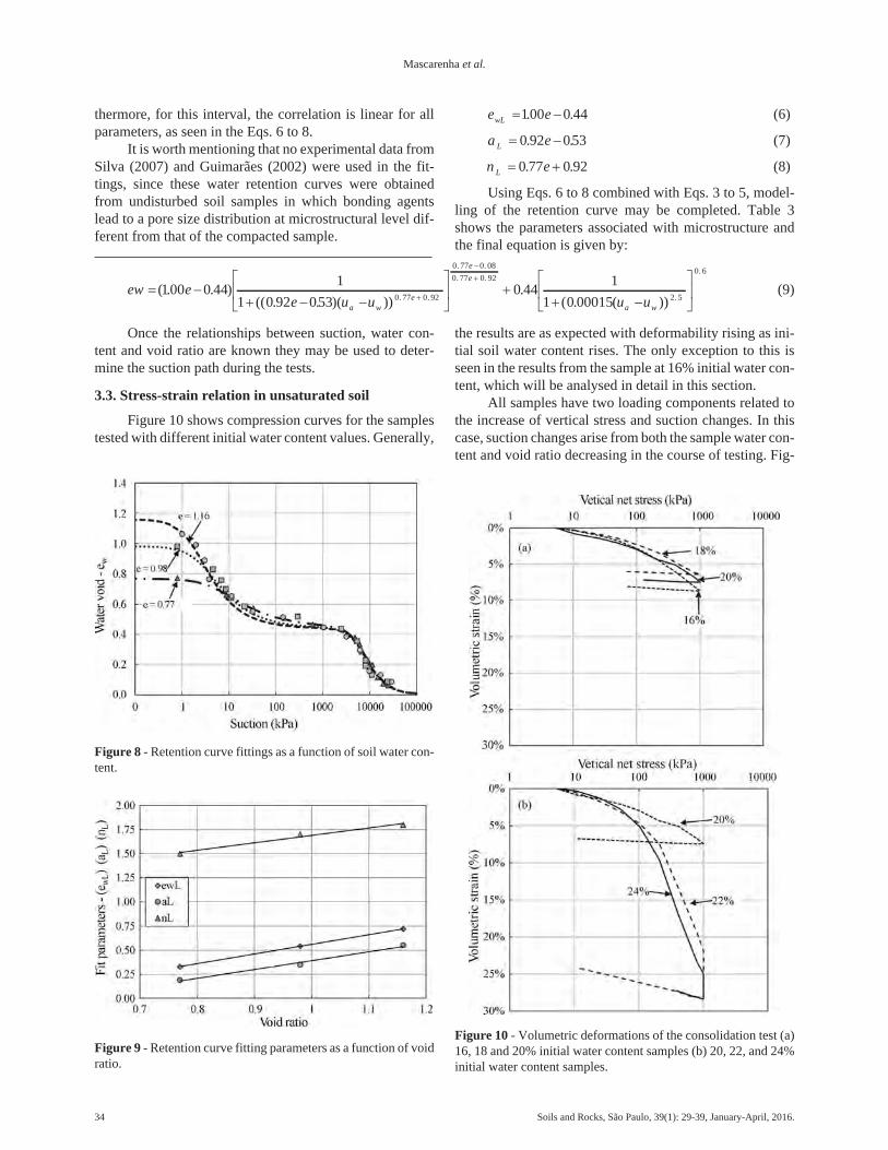
thermore, for this interval, the correlation is linear for allparameters, as seen in the Eqs. 6 to 8.
It is worth mentioning that no experimental data fromSilva (2007) and Guimarães (2002) were used in the fit-tings, since these water retention curves were obtainedfrom undisturbed soil samples in which bonding agentslead to a pore size distribution at microstructural level dif-ferent from that of the compacted sample.
e ewL � �100 0 44. . (6)
a eL � �0 92 053. . (7)
n eL � �0 77 0 92. . (8)
Using Eqs. 6 to 8 combined with Eqs. 3 to 5, model-ling of the retention curve may be completed. Table 3shows the parameters associated with microstructure andthe final equation is given by:
ew ee u ua w
e� �
� � �
��
( . . )(( . . )( )) . .
100 0 441
1 0 92 053 0 77 0 92��
�
�
� �
�
�
0 77 0 08
0 77 0 92
20 44
1
1 0 00015
. .
. .
.( . ( ))
e
e
a wu u .
.
5
0 6�
��
�
(9)
Once the relationships between suction, water con-tent and void ratio are known they may be used to deter-mine the suction path during the tests.
3.3. Stress-strain relation in unsaturated soil
Figure 10 shows compression curves for the samplestested with different initial water content values. Generally,
the results are as expected with deformability rising as ini-tial soil water content rises. The only exception to this isseen in the results from the sample at 16% initial water con-tent, which will be analysed in detail in this section.
All samples have two loading components related tothe increase of vertical stress and suction changes. In thiscase, suction changes arise from both the sample water con-tent and void ratio decreasing in the course of testing. Fig-
34 Soils and Rocks, São Paulo, 39(1): 29-39, January-April, 2016.
Mascarenha et al.
Figure 8 - Retention curve fittings as a function of soil water con-tent.
Figure 9 - Retention curve fitting parameters as a function of voidratio.
Figure 10 - Volumetric deformations of the consolidation test (a)16, 18 and 20% initial water content samples (b) 20, 22, and 24%initial water content samples.

ure 11 shows water content and suction variation for eachsample during the test. Furthermore, these paths are com-pared with the water retention curves, which allow under-standing particular aspects to be discussed along this sec-tion. The paths shown in Fig. 11 were obtained usingEqs. 1, 2 and 9.
An analysis of Fig. 11 shows that although the sam-ples have the same structure, the effect of water contentvariation is different in each case. For example, in thehigher (22% and 24%) water content samples there is out-flow of water from soil macrostructure, while in the lowerwater content (16%) sample, water flows out of the micro-structure.
This factor helps to explain two aspects observed inthe soil behaviour shown in Fig. 10: different behaviour forsamples with different water content and the fact that the16% water content sample showed larger volumetric defor-mations than the 18% and 20% water content samples.
On the other hand, the higher water content samples(24% and 22%) show low suction values throughout thetest: for the 24% water content sample suction ranges from7 to 30 kPa and for 22% from 11 to 78 kPa. Despite theshort range of suction values, the samples experiences ac-centuated collapse due to saturation, as seen in Fig. 10,which is associated with the pore-size distribution, as ex-plained in the following.
When suction is reduced to zero by saturating the 22and 24% initial water content samples, its effect are experi-enced by the macropores range as shown in Fig. 11. Thussuction plays a key role in the soil structural stability, sinceits reduction leads to closing macropores and therefore vol-umetric collapse.
Figure 12 shows the distribution of pores in the soilobtained by indirect measurements using the methodologyreported by Mascarenha (2008) and Otálvaro (2013) fordifferent void ratios. Note that the PSD also helps to ex-plain why the suction value associated with macroporeair-entry (AEVL) for this soil is so low.
It is worth noting that Figs. 11 and 12 justify what wassaid previously about the effect of loading being significantonly for the macropores range while the microstructure re-mains constant after different types of loading.
The other aspect to be considered is that the processof water outlet for the 16% water content sample starts atthe micropores level. Suction values for this sample rangedfrom 1480 to 4445 kPa. The high suction value associatedto this sample should increase soil stiffness, as described inseveral studies such as Alonso et al. (1990). However, sincethese suction values led to outflow of water from the micro-pores, another phenomenon should be considered - the con-traction of the clay clusters that form the microstructure.
Alonso et al. (1999) mentioned that soil macrostruc-tural response is strongly influenced by microstructural be-haviour. A simpler way of evaluating the influence of themacrostructural response caused by microstructure varia-tion will be presented, through a formulation, and subse-quently discussed.
Other aspects for interpretation of the results inFig. 10 are seen in Fig. 13, which shows net vertical stressand suction paths for all samples. The data shows that al-though all the samples have similar variations in water con-tent (about 0.05), the effect on suction values depends onwhether this variation takes place in the soil microstructureor macrostructure as mentioned previously.
An uncertain point in relation to obtaining suctionvalues from the methodology presented is that the water re-tention curves were carried out on mixed (wetting and dry-ing) paths. The water retention curves obtained by Otálvaro(2013) for a soil from Brasilia with similar physical andmineralogical characteristics of the soil studied in this pa-per showed hysteresis. The present study ignored hysteresiseffect and therefore if this behaviour is present in the soilstudied it was not taken into account when determining itscompressibility parameters.
Soils and Rocks, São Paulo, 39(1): 29-39, January-April, 2016. 35
Alternative Method for Analysing Hydromechanical Behaviour of Unsaturated Soils
Figure 11 - Water retention curve - water content agains suction.
Figure 12 - Changes in pore size density functions of a collapsiblesoil.

3.4. Obtaining constitutive parameters
Figure 14 shows the void ratio-effective stress curvefor the saturated condition. In this case, all volumetricchange is associated with vertical loading. Therefore thefollowing parameters associated with constitutive modelssuch as Cam-clay or Barcelona Basic Model (Alonso et al.,1990) may be obtained: pre-consolidation stress for satu-rated conditions (p0
*), elastic stiffness parameter (k), andplastic stiffness parameter for saturated condition (�0).
However, the results shown in Fig. 10, in which thereis no direct suction control, in principle, cannot be used todefine constitutive model parameters, but may be used toenhance interpretation of soil behaviour.
The volumetric strain found for consolidation testingof the 16% initial water content sample was larger than thatof samples with 18 and 20% initial water content. The rea-
son for this is associated with suction changes leading tocontraction of microstructure, as discussed previously.
In order to separate strain due to loading from that dueto contraction of the 16% water content sample micro-structure, it will be assumed there is no plastic deformationdue to loading, only elastic deformations, whereas suctionchanges produces elastic and plastic deformations(Fig. 15).
Although the hypothesis cannot be proven from theresults presented in this paper, it will reveal helpful in un-derstanding soil behaviour and obtaining a set of parame-ters to simulate the paths used.
Figure 15a shows the variation of the sample void ra-tio due to suction change alone, in accordance with theabove assumption. Based on this curve, the Barcelona Ba-sic Model constitutive parameters for suction changes maybe obtained (Alonso et al., 1990): hardening parameter (s0),
36 Soils and Rocks, São Paulo, 39(1): 29-39, January-April, 2016.
Mascarenha et al.
Figure 13 - Variation of suction values during consolidation testsfor samples with different water contents.
Figure 14 - Consolidation curve for a saturated sample.
Figure 15 - Consolidation tests -sample at 16% water content: a) Variation of void ratio with net stress; b) Variation of void ratio withsuction.

elastic stiffness parameter for change in suction (ks) andplastic stiffness parameter for change in suction (�s).
All parameters required by the Barcelona BasicModel to reproduce the paths shown in Fig. 10 are pre-sented in Table 4. The parameters obtained by Peixoto(1999) for the same soil in its natural (or undisturbed) stateare also shown. The values match quite well, particularlygiven the fact that the samples used were in different condi-tions.
Figure 13 shows hypothetical LC (loading-collapse)and SI (suction increase) yield surfaces obtained using pa-rameters from Table 4. This figure clearly shows that 16%initial water content sample would be yielding by reachingthe SI. In contrast, 22% and 24% initial water content sam-ples would quickly reach LC and be deformed by verticalstress alone. The 18% initial water content sample onlyreaches LC and SI for high stress levels and the 20% initialwater content sample does not touch SI and is always tan-gential to LC, although it does reach LC at high levels ofloading, with strain occurring due to vertical stress.
In order to validate the model parameters shown inTable 4, test simulations were performed to obtain the re-sults shown in Figs. 16 to 18. In general, the results ob-tained with the parameters match experimental results quitewell. Furthermore, in the 16% and 18% initial water con-tent samples there are two inflection points in the fittings ofthe consolidation curve. This is due to a fact that loadingstabilization times were not constant, thus causing differentvariations of suction in the course of the test.
Another problem observed in the fittings was that the22% initial water content sample showed less collapse thanthe simulation.
A point to note is that if the variation of suction valuesin the course of the consolidation test were not taken intoaccount, a consistent fitting could not be obtained for tworeasons. One is that, although the 16% initial water contentsample has a higher initial suction value, it shows morestrain than the 18% and 20% initial water content samples,
Soils and Rocks, São Paulo, 39(1): 29-39, January-April, 2016. 37
Alternative Method for Analysing Hydromechanical Behaviour of Unsaturated Soils
Figure 16 - Experimental results from consolidation tests andmodel simulations 16% and 18% initial water content samples.
Table 4 - Barcelona Basic Model (BBM) parameters.
Author Stress Elastic Plastic volumetric compressibility
pc (kPa) p0* (kPa) s0 (kPa) s �0 �sr � (kPa��)
Present study 7.5 70 2250 0.002 0.02 0.20 0.20 0.50 0.007
Peixoto (1999) 20 50 - 0.02 - 0.32 - 0.50 0.01
Figure 18 - Experimental results from consolidation tests andmodel simulations - 24% and saturated initial water content sam-ples.
Figure 17 - Experimental results from consolidation tests andmodel simulations -20% and 22% initial water content samples.

which was due to the large variation in suction during test-ing and these strain occurring in the microstructure, result-ing in permanent deformations.
The second reason is that, the collapse due to floodingunder 1000 kPa stress in the 22% and 24% initial water con-tent samples would be underestimated, since both samplespresent initial suction of around 10 kPa, but reached 78 and30 kPa of suction respectively before flooding, due to de-crease of water content. Note that the underestimation ofcollapse due to assuming constant water content is greaterthan from the use of retention curve in mixed (wetting anddrying) paths to estimate suction values in the course ofconsolidation tests.
4. Conclusions
In the consolidation tests performed assuming con-stant water content, suction change due to evaporation ofwater and reduction of voids is not considered. Thus, soilshrinking due to increased suction is associated with the in-crease of vertical stress. In some cases, this may be wronglyreflected in the value of the compressibility coefficient.
The water content control test described in this paperproved to be efficient at obtaining water content valuesover the test period, and values estimated by the methodproposed were similar to those measured at the end of thetest.
Additionally, a water retention curve could be ob-tained for different void ratios showing that the variation ofvoid ratio affecting soil suction values is only significant inthe soil macrostructure.
Suction changes due to water evaporation rate and re-duced voids was incorporated in the estimation of constitu-tive parameters and proved quite adequate, which wasconfirmed by simulations of the experimental data.
The evaporation rate for the 22% and 24% initial wa-ter content samples must be higher than for a 20% sample,which means that soil water content before flooding thesample was smaller than the estimated value. Additionally,the water retention curve used to estimate suction was ob-tained from a wetting path, whereas in the consolidationtests they were estimated from a drying path. Both factorscombined result in estimated suction lower than actual suc-tion, which would lead to underestimating collapse.
Finally, it is important to note that these parameterswere obtained by means of simple testing: filter paper, wa-ter content control test and consolidation tests.
References
ABNT (1990). Consolidation Test - NBR 12007. Rio de Ja-neiro, Brazil, 13 p.
Alonso, E.; Gens, A. & Josa, A. (1990). A constitutivemodel for partially saturated soils. Géotechnique,40(3):405-430.
Alonso, E.; Vaunat, J. & Gens, A. (1999). Modelling themechanical behaviour of expansive clays. EngineeringGeology, 54(1):173-183.
Alonso, E.; Romero, E. & Hoffmann, C. (2011). Hydro-mechanical behaviour of compacted granular expansivemixtures: experimental and constitutive study. Géo-technique, 61(4):329-344.
Alonso, E.E.; Pinyol, N.M. & Gens, A. (2013). Compactedsoil behaviour: initial state, structure and constitutivemodelling. Géotechnique, 63(6):463-478.
Araki, M.S. (1997). Aspects Related to Collapsible and Po-rous Soils of Federal District. Dissertation G.DM-040A/957, Department of Civil Engineering, Univer-sity of Brasília, Brasília, 121 pp.
Bishop, A.W. (1959). The principle of effective stress. lec-ture delivered in Oslo, Norway in 1995. TekniskUkeblad, 106(39):859-863.
Buenfil, C.M.B. (2007). Hydromechanical Behavior ofCompacted Clay. Doctoral Thesis, Department of Geo-thecnics and Cartography Engenharia, Politécnica Uni-versity of Catalonia, 466 pp.
Camapum de Carvalho, J.; Crispel, J.J.; Mieussens, C. &Nardone, A. (1987). Reconstitution of Samples Labora-tory - Theory and Practice. Research Report, LPC No.145, Regional Laboratory of Toulouse, Toulouse, 88 p.
Camapum de Carvalho, J.; Mortari, D.; Araki, M.S. &Palmeira, E.M. (1994). Behavior of colapsible and po-rous clay of Brasília, Distrito Federal. Proc. X BrazilianCongress on Soil Mechanics and Foundation Engi-neering, Foz do Iguaçu, v. 3, pp. 1157-1163.
Camapum de Carvalho, J. & Leroueil, S. (2000). Norma-lizad characteristic curve. 32nd Annual Paving Confer-ence, Brasília, v. 1, pp. 96-106.
Cardoso, F.B.F (1995). Chemical, Mineralogical andMicromorphological Analysis of Collapsible TropicalSoils and Study of the Dynamics of Collapse. Disserta-tion G.DM-026A/95, Department of Civil Engineering,University of Brasília, Brasília, 140 p.
Della Vecchia. G.; Jommi, C. & Romero, E. (2012). Afully-coupled elastic-plastic hydromechanical modelfor compacted soils accounting for clay activity. Inter-national Journal for Numerical and Analytical Methodsin Geomechanics, 37(5):503-535.
Durner, W. (1994). Hydraulic conductivity estimation forsoils with heterogeneous pore structure. Water Resour-ses Res., 30(2):211-223.
Fredlund, D.G.; Morgenstern, N.R. & Widger, R.A.(1978). The shear strength of unsaturated soils. Cana-dian Geotechnical Journal, 15(3):313-321.
Gens, A. & Alonso, E. (1992). A framework for the behav-iour of unsaturated expansive clays. Canadian Geo-technical Journal, 29(6):1013-1032.
Guimarães, R.C. (2002). Lateritic Soil Profile BehaviorApplied to the Study of Bored Piles Performance. Dis-sertation G.DM-091A/02, Department of Civil and En-
38 Soils and Rocks, São Paulo, 39(1): 29-39, January-April, 2016.
Mascarenha et al.

vironmental Engineering, University of Brasilia,Brasilia, 183 p.
Marinho, F.A.M. (1994). Filter paper method to measuresuction . Proc. X Brazilian Congress on Soil Mechanicsand Foundation Engineering, Foz do Iguaçu, v. 2,pp. 515-522.
Matyas, E.L. & Radhakrishna, H.S. (1968). Volume chan-ge characterists of partially satured soils. Geothech-nique, 18(4):432-448.
Mascarenha, M.M.A. (2008). Influence of Microstructureon Hydro-Mechanical Behavior of a Silty Clay Unsatu-rated. Doctoral Thesis, Publication G.TD-056/08, De-partment of Civil Engineering, University of Brasília,Brasília, 158 p.
Otálvaro, I.F.C. (2013). Hydromechanical Behavior of aCompacted Soil Tropical. Doctoral Thesis, GraduateProgram in Geotechnical Engineering, Department ofCivil and Environmental Engineering, Faculty of Tech-nology, University of Brasilia, 122 p.
Peixoto, R.J. (1999). Modeling Constitutive of Collapsibleand Porous Clay Behavior of Federal District. Disserta-tion, Department of Civil and Environmental Engi-neering,, University of Brasilia, Brasilia, 191 pp.
Romero, E.; Hoffmann, C.; Castellanos; E., Suriol, J.&Lloret, A. (2005). Microstructural changes of com-pacted bentonite induced by hydro-mechanical actions.Advances in Understanding Engineered Clay Barriers,E.E., Alonso & A. Ledesma (eds.) Taylor & FrancisGroup, London, pp. 193-202.
Romero, E. & Vaunat, J. (2000). Retention curves of de-formable clays. Tarantino & Mancuso (eds), Experi-mental Evidence and Theoretical Approaches inUnsaturated Soils, Balkema, Rotterdam, pp. 91-106.
Sheng, D.; Sloan, S.W. & Gens, A. (2004). A constitutivemodel for unsaturated soils: thermomechanical andcomputational aspects. Computational Mechanics Jour-nal, 33(6): 453-465.
Silva, J.P. (2007). Preliminary Studies for the InfiltrationTrenches Implementation. Dissertation G.DM-154A/07, Department of Civil and Environmental Engi-neering, University of Brasilia, Brasilia, 183 p.
Silva, M.T.M.G. (2009). Methodology for Determinationof Unsaturated Soils Parameters Using Tests withKnown Humidity. Dissertation, Department of CivilEngineering, University of Brasília, Brasília, 98 p.
Simms, P.H. & Yanful, E.K. (2002). Predicting soil-watercharacteristic curves of compacted plastic soils frommeasured pore-size distributions. Géotechnique,52(4):269-278.
Van Genuchten, M.Th. (1980). A closed-form equation forpredicting the hydraulic conductivity of unsaturated
soils. Soil Science Society of America Journal,44(5):892-898.
Vaunat, J.; Romero, E. & Jommi, C. (2000).An elasto-plastichydromechanical model for unsaturated soils.Tarantino & Mancuso (eds), Experimental Evidenceand Theoretical Approaches in Unsaturated Soils, Bal-kema, Rotterdam, pp. 121-138.
Wheeler, S.J.; Sharma, R.S. & Buisson, M.S.R. (2003).Coupling of hydraulic hysteresis and stress-strain be-haviour in unsaturated soils. Géotechnique, 53(1):41-54.
List of SymbolsAEV: air entry valuesCOV: coefficient of variatione: void ratioew: soil water contentewL: macropore void ratioewS: micropore void ratioGs: specific gravityk: elastic stiffness parameterks: elastic stiffness parameter for change in suctionmL: slope of the line that relates transition water content andsuctionmS: slope of the line that relates water content and suctionafter hygroscopic soil water content valuenL: slope of the line that relates macropore water contentand suctionnS: slope of the line that relates macropore water contentand suctionpc: reference stressp0
*: pre-consolidation stress for saturated conditionsPSD: Pore Size Densityr: parameter defining the maximum soil stiffnesss0: hardening parametert: time elapsed from start of testingw: water contentwc: corrected water contentwcom: compaction water contentwi: initial water contentwk: corrected water content for time 240 minwL: liquid limit indexwM: macroscopic water contentwm: microscopic water contentwP: plastic limit index�L: parameter related to air-entry value for macropores�S� parameter related to air-entry value for micropores�� parameter controlling the rate of increase of soil stiffnesswith suction�0: plastic stiffness parameter for saturated condition�s: plastic stiffness parameter for change in suction
Soils and Rocks, São Paulo, 39(1): 29-39, January-April, 2016. 39
Alternative Method for Analysing Hydromechanical Behaviour of Unsaturated Soils


Recent Developments and Limitations of the SFG Model
D. Sheng
Abstract. The SFG model was proposed in attempt to provide a consistent description of the stress-strain behaviour ofunsaturated soils, including compacted soils and soils dried from slurry. It differs from existing models mainly through twoaspects: a consistent description of volume change, yield stress and shear strength behaviour of unsaturated soils and asmooth and natural transition between saturated and unsaturated states. The model has attracted significant attention sinceit was first proposed and has been extended to cover coupled hydro-mechanical behaviour, hysteretic water retentionbehaviour and density-dependency. This paper presents a summary of the latest developments of the model, as well as theaspects that require further refinements.Keywords: SFG model, unsaturated soils, volume change, shear strength, hydro-mechanical coupling.
1. Introduction
The SFG model proposed by Sheng et al. (2008a) at-tempts to provide a consistent and unified description ofvolume change, yield stress, shear strength and hydraulicbehaviour of unsaturated soils, including compacted soilsand soils dried from slurry. It is established in the space ofthe independent stress variables, namely net stress andmatric suction. However, unlike models using similarstress variables, the SFG model provides a smooth and nat-ural transition between saturated and unsaturated states.The model has attracted significant attention since it wasproposed in 2008. It has been further extended to cover soilbehaviour such as hydro-mechanical interaction, hystereticwater retention, and density dependency. However, thismodel also has a number of limitations that require furtherimprovements. This paper presents a summary of the latestdevelopments of the SFG model and the areas where themodel falls short of real soil behaviour.
2. The SFG Model
The essential ingredient of the SFG model is its vol-ume change equation. According to the model, the volumechange of a soil can be caused by a change of net stress or achange of suction. For normally consolidated soils underisotropic stress states, the volume change equation takes thefollowing form:
dvdp
p f ss
ds
p f svp vs� �
��
�� �
( )( )
( )(1)
where is the specific volume and v = 1+e, e is the void ratio,p is the mean net stress and p = p - ua, p is the mean stress, ua
is the pore air pressure, uw is the pore water pressure, s is thesoil suction and s = ua – uw, �vp is the soil compressibility interms of stress changes, and �vs is the soil compressibility in
terms of suction changes. The function f(s) represents theinteraction between stress and suction and was simply set tos in the original SFG model (Sheng et al., 2008a). However,more advanced forms could be used, as suggested by Sheng(2011).
The parameter �vp can be determined from normalcompression lines (NCL) for s = 0. It is the same as theslope (�) of NCL in e-lnp plots that are commonly used forsaturated soils. In its simplest form this parameter can betreated as a constant for one soil, but more realistically itshould be a function of suction. The parameter �vs is a func-tion of suction. Its initial value is the same as �vp for suctionsbelow the transition value between saturated and unsatu-rated states, but it approaches zero as suction increases toinfinite. The following simple equation was used in Shenget al. (2008b):
��
�vs
vp sa
vpsa
sa
s s
s
ss s
��
�
�
�(2)
where ssa is the transition suction and its definition isslightly different from the air entry value (see Sheng et al.,2008a).
The volume change model defined by Eqs. 1 and 2 isthe foundation of the SFG model. Zhou & Sheng (2009)provided a systematic validation of the volume changeequation for compacted and air-dry soils. The yield stressand shear strength criteria in the SFG model are all based onthis volumetric model. The yield stress function for a slurrysoil can be derived from the volume change equation (as-suming that the plastic volumetric strain is only hardeningvariable) and it also defines the apparent tensile strength ofthe soil:
Soils and Rocks, São Paulo, 39(1): 41-49, January-April, 2016. 41
Daichao Sheng, Professor, School of Engineering, The University of Newcastle, NSW 2308, Australia, and School of Civil Engineering, Central South University, Changsha,410072, China. e-mail: [email protected] Article, no discussion.

p
s s s
s ss
ss s
sa
sa sa
sa
sa0 �
� �
� � �
�
� ln
(3)
The loading-collapse equation for collapsible soils(e.g. compacted soils) can also be derived from the volumechange equation:
p
p s s s
p
pp f s s s
s
sc
cn sa
cn
c
c sa sa
sa
�
� �
� � �
���
�
��
0
0
0
0 ( ) ln � �
�
� s ssa
(4)
where pc is the yield stress at an arbitrary suction, pcn0 is theyield stress at zero suction, pc0 is a constant.
Note that there is no ‘suction-increase’ or ‘suction-decrease’ yield surface in the SFG model. The plastic volu-metric strain caused by drying a soil to historically highsuction is automatically covered in the apparent tensilestrength function p0.
The apparent tensile strength function and the load-ing-collapse function can be incorporated into existing con-stitutive models for saturated soils. For example, if themodified Cam clay model is used for saturated soil behav-iour, the yield function can be generalised to unsaturatedstates along the suction axis:
f q M p p p pc� � � � �2 20 0( )( ) (5)
where f is the yield function in the stress space, q is the devi-ator stress, M is the slope of the critical state line in q - pspace, and p0 and pc are defined above.
Using the shear strength criterion proposed byFredlund et al. (1978):
� � � �� � � � �[ ' ( ) tan ' ] [( ) tan ]c u u un a a wb (6)
The friction angle due to suction in the SFG modelcan be derived from the apparent tensile strength equationand is given by
tan
tan '
tan ' ln�
�
�b
sa
sa sa
sa
sa
s s
s
s
s
s
s
ss s
�
�
�
���
�
��� �
�
�
(7)
In the equations above, � is the shear strength, �n is thenormal stress on the failure plane, �’ is the effective frictionangle of the soil, and �b is the frictional angle due to suction.Equation 7 can be used to predict the change of the shearstrength against suction.
In the original SFG model, hydro-mechanical cou-pling was only considered from the aspect that suction af-fects the stress-strain behaviour. This was extended to con-sider the effect of stress on the water retention behaviour bySheng & Zhou (2011) by incorporating the following con-stitutive equation:
dS EdsS
nS
p f sdpr
rr
m vp� � ��
( )( )
1�
(8)
where Sr is the degree of saturation, n is the porosity, and mis a fitting parameter. Function E in Eq. 8 refers to the gradi-ent of the soil-water characteristic curve (SWCC,dSr = Eds) and may also be multi-valued in a piece-wiseequation, dependent on the suction path. Because Eq. 8 is inan incremental form, integration of the equation requiresone specific SWCC that corresponds to a reference initialvoid ratio. In other words, the conventional SWCC equa-tion is only used for the reference initial void ratio and thenew SWCC for a new initial void ratio is obtained by inte-gration of Eq. 8. Sheng & Zhou (2011) gives the details onhow to use an existing SWCC equation for different initialvoid ratios.
We note that replacing Eq. 1 into Eq. 8 leads to:
dS Ep f s
S
nS ds
S
eS der
vs rr
m rr
m� ��
�
���
�
��� � �
�
( )( ) ( )1 1 (9)
The above equation clearly indicates that the Sr - s re-lationship for constant void ratio (de = 0) is not the same asthe SWCC equation (dSr = Eds). Equations 8 and 9 areequivalent and interchangeable.
Equations 1-9 are the main equations of the SFGmodel. These equations sufficiently define the volumechange, yield stress, shear strength and coupled hydro-mechanical behaviour of unsaturated soils. In the follow-ing, we will first discuss what the SFG model can do andthen outline where it falls short.
3. Predictions of the SFG Model
The main advantage of the SFG model is that it isbased on a simple volume change equation and is able toprovide a consistent framework for volume change, shearstrength and coupled hydro-mechanical behaviour of unsat-urated soils.
3.1. Volume change behaviour
The volume change caused by suction increase (dry-ing) can be predicted by Eqs. 1 and 2 directly. Figure 1shows the SFG prediction compared with experimental ofMariho et al. (1995). There are three parameters involvedin the prediction: the compressibility of saturated soil (�vp
and �vp) and the transition suction (air entry value in thiscase). The figure shows that the SFG model is capable ofcapturing the volume change during drying.
The volume change caused by stress change can alsobe predicted by Eq. 1. Figure 2 compares the SFG predic-tions with the experimental data of Thu et al. (2007). Thedata were obtained from isotropic compression tests underconstant suctions on compacted Kaolin. The predicted re-sults match very well the experimental data, indicating that
42 Soils and Rocks, São Paulo, 39(1): 41-49, January-April, 2016.
Sheng

Soils and Rocks, São Paulo, 39(1): 41-49, January-April, 2016. 43
Recent Developments and Limitations of the SFG Model
Figure 1 - Volume change during drying for Brown London Clay (data of Marinho, et al., 1995).
Figure 2 - Predictions of isotropic compression curves for compacted kaolin specimen (data by Thu et al., 2007).

the SFG model is capable of predicting the volume changecaused by stress change.
The volume change during wetting is more complex.It may involve the expansion of the loading-collapse yieldsurface, or so-called hardening. In this case, a completeconstitutive model is needed to predict the volume change.Figure 3 was taken out from Sheng et al. (2008a) and showsthe predicted volume collapse during wetting of compactedPearl clay. The compacted sample (point A in Fig. 3) wasfirst dried to a constant suction (point B) and then com-pressed to different stress levels (Points D, E, F, G, H, I),followed by wetting under constant net mean stresses fullsaturation (Points D’, E’, F’, G’, H’, I’). Figure 3 shows thatthe predicted collapse volume depends on the stress levelwhere the wetting takes place. The prediction was not com-pared with experimental data due to the lack of detailed soilparameters. However, the experimental data was shown onthe lower left corner, to indicate the qualitative agreementbetween the prediction and the experimental data.
3.2. Shear strength
In the SFG model, the shear strength behaviour is anatural outcome of the volume change equations and does
not need any additional definition or material parameters.Nevertheless, the model is capable to predict the shearstrength variation with suction to a reasonable degree. Fig-ure 4 shows the predicted shear strength variation with suc-tion, compared with the experimental data by Vanapalli etal. (1996). The tests and predictions are for direct sheartests. Figure 5 compares the predictions with experimentaldata from triaxial tests. The results in both figures indicatethat the SFG model provides a reasonable prediction of un-saturated soil shear strength.
3.3. Hydro-mechanical coupling
The extended SFG model by Sheng & Zhou (2011)and Zhou et al. (2012a) provides a complete couplingmechanism for the interaction between stress-strain andwater retention behaviour. The effects of suction and de-gree of saturation on stress-strain and strength behaviourhave already been demonstrated above. The effects ofstress on water retention behaviour are demonstrated be-low.
Considering the soil water characteristic curves (orSWCC) under constant stresses, the effect of stress is pri-marily reflected through its effect on the initial soil density
44 Soils and Rocks, São Paulo, 39(1): 41-49, January-April, 2016.
Sheng
Figure 3 - Predicted volume collapse during the final wetting paths (experimental results of Sun et al. (2007) shown on the lower leftcorner).

or initial soil void ratio. Figure 6 shows the predicted andmeasured SWCCs for soils compacted to different initialvoid ratios. The predicted SWCCs are shown as solid cur-ves. The fitting parameter m in Eq. 8 is set to 0.03. TheSWCC for initial ratio of 0.517 was obtained using vanGenuchten equation with fitting parameters given in Sheng& Zhou (2011). The predicted SWCCs compares very wellwith the measured data, indicating that the proposed modelcan capture the shift of SWCC with initial void ratio.
Figure 7 further demonstrates the capability of theSFG model in predicting the effects of initial void ratio onthe water retention behaviour. The soil tested was a siltysand from a Saskatchewan Department of Highway borrowpit (Huang et al., 1998). The air-dried silty sand was mixedwith distilled water to prepare slurry specimens for the ex-
Soils and Rocks, São Paulo, 39(1): 41-49, January-April, 2016. 45
Recent Developments and Limitations of the SFG Model
Figure 4 - Shear strength vs. suction during direct shear tests (data by Vanapalli et al., 1996).
Figure 5 - Shear strength vs. suction during triaxial compression tests (data by Wheeler & Sivakumar, 2000).
Figure 6 - Measured and predicted SWCCs (data after Vanapalliet al., 1999).

perimental program. Six initially slurry specimens wereone-dimensionally preconsolidated under different pres-sures to obtain different initial void ratios for the water re-tention tests. The test results are replotted in the Se - s planetogether with the predictions of Eq. 8, as shown in Fig. 7.The water retention test data for an initial void ratio 0.525were used to calibrate the reference van Genuchten SWCCequation (Zhou et al., 2012a). The fitting parameter m inEq. 8 was set to 0.2. As shown in Figure 7, the predictedSWCCs agree very well with the experimental SWCCs.The shifting of the SWCC due to changes in the initial den-sity is well portrayed by the SFG model.
4. Limitations of the SFG Model
4.1. Loading collapse surface for coupled hydro-mecha-nical formulation
One common limitation of models defined in thestress - suction space is related to the coupling between wa-ter retention and stress-strain behaviour. The SFG model isno exception for this shortcoming.
It is commonly accepted that the water retention cur-ve of a soil depends on the stress level and the initial state(such as initial density) of the soil. Under the same stresslevel, the main drying curve shifts towards higher suctionregion with decreasing initial void ratio (Fig. 6). For the
46 Soils and Rocks, São Paulo, 39(1): 41-49, January-April, 2016.
Sheng
Figure 7 - Measured and predicted SWCCs for a silty sand with different initial void ratios (data after Huang et al., 1998).

same soil, the main drying curve shifts towards higher suc-tion region when the stress level applied to the soil in-creases. That means the air entry suction is not constant forthe same soil, but depends on the initial void ratio of the soiland the stress level applied to the soil. On the other hand,the loading-collapse yield curve experiences a curvaturechange around the transition suction such as the air entryvalue, which means the shape of the loading-collapse curvedepends on the air entry value. Because of the dependencyof the air entry value on the stress level and initial conditionof the soil, the shape of the load-collapse curve would thendepend on the stress level and initial condition of the soil,which is not acceptable for the definition of a yield surface.The yield surface must be independent of the stress states itencloses.
This limitation is common to all models defined in thestress - suction space, irrespective of the stress variablesused (Fig. 8). It should also be noted that the transition suc-tion appears implicitly in all models, even though somemodels set it to zero (such as in BBM of Alonso et al.,1990). As mentioned in Sheng (2011), different degrees ofsaturation are only states of the soil and the transition fromsaturated to unsaturated states (for example, a change ofpore water pressure from 10 kPa to -10 kPa) should alwaysbe allowed in a model. Therefore it is not possible to get ridof the transition suction. The conclusion is then that the
loading-collapse yield surface becomes meaningless in thestress - suction space if the water retention behaviour isconsidered to depend on stress level or initial condition ofthe soil.
A possible solution to the above shortcoming is to de-fine the loading-collapse curve in terms of a variable alter-native of suction. In the model by Wheeler et al. (2003), theloading-collapse curve is defined in the space of effectivestress vs. modified suction, where it does not have an inflec-tion point (Fig. 9a). Such a definition essentially impliesthat the water retention curve when plotted in terms of mod-ified suction and degree of saturation is independent ofstress levels or initial density of the soil. This implicationremains to be further validated experimentally. In themodel of Zhou et al. (2012b, 2012c), the loading-collapsecurve is defined in the space of effective stress vs. degree ofsaturation and there is no inflection point along the load-ing-collapse curve in this space (Figure 9b). The load-ing-collapse curves in these models are then independent ofthe stress or suction path within the loading-collapse curvesand are hence more meaningful.
4.2. Compression under constant suction
The current version of the SFG model predicts typicalnormal compression curves under constant suctions asshown in Fig. 10. In reality, compression under constant
Soils and Rocks, São Paulo, 39(1): 41-49, January-April, 2016. 47
Recent Developments and Limitations of the SFG Model
Figure 9 - Loading-collapse yield surface defined in alternative spaces.
Figure 8 - Loading-collapse yield surface in suction-stress space.

suction, especially under a low suction, results in increaseof degree of saturation. In other words, it is possible to com-press an unsaturated soil under constant suction to full satu-ration. A more realistic compression curve for constantsuction should then converge to the saturated normal com-pression line, as shown by the dashed curve in Fig. 10.
This limitation can in theory be overcome by using acompressibility parameter (�vp) that increases with increas-ing suction. However, such a modification would signifi-cantly complicate the integration of incremental equationsin the SFG model. In addition, it would not provide asmooth convergence to full saturation. A better solution is,as suggested in Zhou et al. (2012b), that the compressibilityparameter is assumed to decrease with decreasing degree ofsaturation. With such an assumption, compression underconstant suction would result in increase in the degree ofsaturation and hence decrease in the soil compressibility.However, as pointed out in Sheng (2011), it should beavoided to have both suction and degree of saturation in thevolume change equation, due to the hysteretic relationshipof the two variables. Introducing the degree of saturationinto the volume change equation would require the elimina-tion of suction from it. The effects of suction have then tobe considered through the stress variable - effective stress.This is the fundamental reason why Zhou et al. establishtheir model in the space of effective stress vs. the degree ofsaturation.
Other limitations of the SFG model include the non-conservative behaviour of the elastic zone, the difficulty ofusing a more advanced function f(s) in Eq. 1, and thenon-convexity of the elastic zone, as discussed in Sheng(2011). However, these limitations are not unique to theSFG model and the measures for dealing with them havebeen discussed in detail in Sheng (2011).
5. Summary
The SFG model provides a consistent and unifiedframework for describing volume change, yield stress,
shear strength and coupled hydro-mechanical behaviour ofunsaturated soils. It is established in the space of the inde-pendent stress variables, namely net stress and matric suc-tion. It provides a smooth and natural transition betweensaturated and unsaturated states. The model has been fur-ther extended to cover soil behaviour such as hydro-mecha-nical interaction, hysteretic water retention, and densitydependency. However, this model also has a number oflimitations that require further improvements. One of themost significant limitations is related to the definition of theloading-collapse yield surface when the coupled hydro-mechanical behaviour is considered. This paper has pre-sented a summary of the latest developments of the SFGmodel and the areas where the model falls short of real soilbehaviour.
References
Alonso, E.E.; Gens, A. & Josa, A. (1990). A constitutivemodel for partially saturated soils. Geotechnique,40(3):405-430.
Fredlund, D.G.; Morgenstern, N.R. & Widger, A. (1978).Shear strength of unsaturated soils. Canadian Geotech-nical Journal, 15(3):313-321.
Huang, S.; Barbour, S.L. & Fredlund, D.G. (1998). Devel-opment and verification of a coefficient of permeabilityfunction for a deformable unsaturated soil. CanadianGeotechnical Journal, 35(3):411-425.
Marinho, F.A.M.; Chandler, R.J.; & Crilly, M.S. (1995).Stiffness measurements on an unsaturated high plastic-ity clay using bender elements. In Proceedings of the 1stInternational Conference on Unsaturated Soils, Sep-tember 1995. Paris. A.A. Balkema, Rotterdam, v. 2,pp. 535-539.
Sheng, D. (2011). Review of fundamental principles inmodelling unsaturated soil behaviour. Computers andGeotechnics, 38:757-776.
Sheng, D.; Fredlund, D.G. & Gens, A. (2008a). A newmodelling approach for unsaturated soils using inde-pendent stress variables. Canadian Geotechnical Jour-nal, 45(5):511-534.
Sheng, D.; Gens, A.; Fredlund, D.G. & Sloan, S.W.(2008b). Unsaturated soils: From constitutive model-ling to numerical algorithms. Computers & Geotech-nics, 35:810-824.
Sheng, D. & Zhou, A.N. (2011). Coupling hydraulic withmechanical models for unsaturated soils, CanadianGeotechnical Journal, 48(5):826-840.
Sun, D.A.; Sheng, D. & Xu, X.F. (2007). Collapse behav-iour of unsaturated compacted soil. Canadian Geotech-nical Journal, 44(6):673-686.
Thu, T.M.; Rahardjo, H. & Leong, E.C. (2007). Soil watercharacteristic curve and consolidation behaviour of acompacted silt. Canadian Geotechnical Journal,44(3):266-275.
48 Soils and Rocks, São Paulo, 39(1): 41-49, January-April, 2016.
Sheng
Figure 10 - SFG normal compression lines at different suctions(N = 3, �vp = 0.1, ssa = 10 kPa).

Vanapalli, S.K.; Fredlund, D.G.; Pufahl, D.E. & Clifton,A.W. (1996). Model for the prediction of shear strengthwith respect to soil suction. Canadian GeotechnicalJournal, 33(3):379-392.
Vanapalli, S.K.; Fredlund, D.G. & Pufahl, D.E. (1999). Theinfluence of soil structure and stress history on soil-water characteristics of a compacted till. Géotechnique,49(2):143-159.
Wheeler, S.J.; Sharma, R.S. & Buisson, M.S.R. (2003).Coupling of hydraulic hysteresis and stress-strain be-haviour in unsaturated soils. Géotechnique, 53(1):41-54.
Wheeler, S.J. and Sivakumar, V. (2000). Influence of com-paction procedure on the mechanical behaviour of anunsaturated compacted clay. Part 2: Shearing and con-stitutive modelling. Géotechnique, 50(4):369-376.
Zhou, A.N. & Sheng, D. (2009). Yield stress, volumechange and shear strength behaviour of unsaturatedsoils: Validation of the SFG model. Canadian Geo-technical Journal, 46(8):1034-1045.
Zhou, A.N.; Sheng, D. & Carter, J.P. (2012a). Modellingthe effect of initial density on soil water characteristiccurves, Géotechnique, 62(8):669-680.
Zhou, A.N.; Sheng, D.; Sloan, S.W. & Gens, A. (2012b).Interpretation of unsaturated soil behaviour in the stress- saturation space, I: Volume change and water reten-tion behaviour. Computers and Geotechnics, 43:178-187.
Zhou, A.N.; Sheng, D.; Sloan, S.W. & Gens, A. (2012c).Interpretation of unsaturated soil behaviour in the stress- saturation space, II: Constitutive relationships and val-idations. Computers and Geotechnics, 43:111-123.
Soils and Rocks, São Paulo, 39(1): 41-49, January-April, 2016. 49
Recent Developments and Limitations of the SFG Model


Effectiveness of Capillary Barrier and Vegetative SlopeCovers in Maintaining Soil Suction
H. Rahardjo, S. Krisnanto, E.C. Leong
Abstract. Capillary barrier and vegetative slope covers can be used to improve slope stability during rainfall bymaintaining matric suction in the slope. A study was performed to investigate the effectiveness of capillary barrier system(CBS) and vegetative slope covers (Orange Jasmine and Vetiver grass) in maintaining soil suction. Performance of slopeswith and without slope covers was investigated using field instrumentations and numerical analyses. Laboratory tests wereperformed to measure hydraulic and shear strength properties of the soil, the soils with Orange Jasmine and Vetiver grassroot, and CBS materials. Numerical analyses were performed to investigate the variation of pore-water pressure profiles ata selected location and factor of safety during low, high, and maximum rainfall intensities. Pore-water pressures measuredin the field were used to calibrate the numerical models. Laboratory test results showed that the presence of root increasedthe shear strength of soil. Numerical analyses and field monitoring results showed that the slope with covers can maintainnegative pore-water pressure better than the original slope. Performance of Orange Jasmine, Vetiver grass, and CBS inmaintaining matric suction in the slope is essentially similar during low, high, and maximum rainfall intensities.Keywords: slope covers, stability, soil suction, infiltration, instrumentation.
1. Introduction
Residual soils commonly exist in many tropical areas.These soils are often in the unsaturated condition with neg-ative pore-water pressure (matric suction). The presence ofmatric suction increases shear strength of the soil. There-fore, the presence of matric suction is a favorable conditionfor slope stability. However, rainfall infiltration into slopewill increase pore-water pressure or decrease matric suc-tion in soil, resulting in a decrease in shear strength of thesoil. The decrease of shear strength causes the slope to be-come more prone to failure that is commonly referred to asrainfall-induced slope failure (Pitts 1985; Tan et al., 1987;Brand 1992; Gasmo et al., 2000; Tsaparas et al., 2002).
Capillary barrier system (CBS) is a two-layer systemof soil cover that is designed based on unsaturated soil me-chanics principles. CBS consists of a fine-grained soil layerplaced on top of a coarse-grained soil layer. The contrast insoil-water characteristic curve (SWCC) and permeabilityfunction between these two layers is utilized to create a bar-rier to minimize water infiltration into the underlying soil.
Capillary barrier system (CBS) can be used to miti-gate rainfall-induced slope failures (Ross 1990; Steenhuiset al., 1991; Morel-Seytoux 1993, 1994; Stormont 1996;Morris & Stormont 1997a, 1997b; Khire et al., 2000; Tamiet al., 2004a, 2004b; Yang et al., 2004b; Krisdani et al.,2008). CBS consists of two different soil layers with a sig-nificant difference in their soil-water characteristic curves
(SWCC) and permeability functions that serves to mini-mize water seepage into the underlying layers.
Besides CBS, vegetative cover can also be used tomitigate rainfall-induced slope failure (e.g. Grimshaw1994; Thruong & Gawander 1996; World Bank 1995; Na-tional Research Council 1993). The presence of root can in-crease shear strength of soil (Styczen & Morgan 1995).Orange Jasmine, Murraya exotica L., and Vetiver grass,Chrysopogon zizaniodes, are evergreen vegetations thatcan be planted in a tropical area like Singapore. They canadapt to variation in weather conditions and require mini-mum maintenance. Because of these characteristics, Or-ange Jasmine and Vetiver grass are potential vegetations tobe used as soil covers to overcome rainfall-induced failureproblems in the tropics.
Each slope cover may perform differently in main-taining matric suction. In addition, the performance ofslope cover may differ under different rainfall intensities.Therefore, there is a need to investigate the effectiveness ofcapillary barrier and vegetative slope covers in maintainingsoil suction.
The objective of this study is to compare the perfor-mance of Orange Jasmine and Vetiver grass slope coversand CBS in maintaining matric suction through field mea-surements and numerical analyses. The effect of OrangeJasmine and Vetiver grass roots on soil shear strength isalso investigated through laboratory tests.
Soils and Rocks, São Paulo, 39(1): 51-69, January-April, 2016. 51
H. Rahardjo, Professor, School of Civil & Environmental Engineering, Nanyang Technological University, Blk N1, #1B-36, 50 Nanyang Avenue, 639798, Singapore. e-mail:[email protected]. Krisnanto, Lecturer, Geotechnical Engineering Research Division, Faculty of Civil & Environmental Engineering, Bandung Institute of Technology, Soil Mechanics Labo-ratory, CIBE Building, Jalan Ganesha No. 10, Bandung 40132, Indonesia. e-mail: [email protected]. Leong, Associate Professor, School of Civil & Environmental Engineering, Nanyang Technological University, Blk N1, #1C-80, 50 Nanyang Avenue, 639798, Singa-pore. e-mail: [email protected] Article, no discussion.

2. Site Overview
The geology of Singapore consists of Old Alluviumin the eastern and northeastern regions, the sedimentaryJurong Formation in the western region, and Bukit TimahGranite in the center and northwestern regions.
A slope consists of soil from the Old Alluvium wasselected for this study. The slope has a height of 8.21 m, alength of 22.55 m, and a slope angle of 20°. The slope wasdivided into three sections: the first section was the originalslope covered with cow grass, the second section was cov-ered with Orange Jasmine, the third section was coveredwith Vetiver grass, and the fourth section was covered withCBS. Layout of the slope is shown in Fig. 1. Based on soilinvestigation and laboratory tests, it was found that theslope consists of two layers of residual soils, named as layer1 and layer 2. A relatively thin sub layer with saturated per-meability lower than those of layers 1 and 2 was foundwithin layer 1. Schematic diagrams of each section of theslope are shown in Fig. 2.
3. Design of Slopes and Field Instrumentation
The original slope was covered by cow grass sur-rounded by trench (Fig. 1). The original slope was instru-mented with three Casagrande piezometers and three tensi-ometers (Fig. 2(a)). The piezometers were installed at nearthe crest, middle and near the toe of the slope. The tensiom-eters were labelled as TA3, TB3, and TD3 with a spacing of0.5 m and insertion depths of 0.67 m, 1.29 m, and 1.84 m,respectively (Fig. 2(a)). Polyvinyl chloride (PVC) casingswere installed at the locations of tensiometers and piezo-meters for installing the instruments.
Schematic diagram of the slope covered with OrangeJasmine and Vetiver grass is shown in Fig. 2(b). OrangeJasmine and Vetiver grass were planted in June and Sep-
tember 2009, respectively. In this study, only direct rainfallinfiltration onto the covered slope had to be observed.Therefore, the lateral water flow from the surrounding soilinto the vegetated area must be prevented. To achieve thiscondition, the vegetated areas were surrounded by a trenchand impermeable metal sheets that were installed to600 mm depth from the slope surface (Fig. 2(b)). PVC cas-ings for tensiometers were installed at the planned locationsof tensiometers. Before planting the vegetations, erosionblanket was laid on the slope surface to protect the slopewithin the study area from erosion during rainfall. OrangeJasmine was planted with lateral and down slope spacing of450 mm whereas Vetiver grass was planted with lateralspacing of 250 mm and down slope spacing of 450 mm toavoid overlapping roots between adjacent vegetations. Inthe slope with Orange Jasmine, three tensiometers were in-stalled. The installed tensiometers were labelled as TE4,TA4, and TB4 with a spacing of 0.5 m and insertion depthsof 0.4 m, 0.66 m, and 1.21 m, respectively. In the slope withVetiver grass, three tensiometers were also installed. Theinstalled tensiometers were labelled as TE5, TA5, and TB5with a spacing of 0.5 m and insertion depths of 0.4 m,0.67 m, and 1.24 m, respectively.
Schematic diagram of the slope covered with CBS isshown in Fig. 2(c). To construct the CBS, the slope surfacewas excavated to 540 mm depth below the slope surface.Similar to the slope sections with vegetations, the CBS areawas also surrounded by trench and impermeable metalsheets. A 6.5 mm thick layer of a geosynthetic drainage sys-tem (Secudrain) was used as a separator between the fine-grained layer and the original soil. J-pins of 75 cm and115 cm in length penetrating 54 cm and 75 cm into theground, respectively, were installed. PVC casings for tensi-ometers were installed at the planned locations of tensiom-eters. Geocells were laid on top of the secudrain for con-
52 Soils and Rocks, São Paulo, 39(1): 51-69, January-April, 2016.
Rahardjo et al.
Figure 1 - Layout of the investigated slope.

taining the coarse-grained layer secured by the 75 cm longJ-pins. Recycled concrete aggregate (RCA) as the coarse-grained layer was backfilled into the geocells and com-pacted to a relative density (Dr) between 70%-90% or to the
required dry density (�d) of 1.80 g/cm3. A nonwoven geo-textile TS 80 (TenCate 2011) was used in the capillary bar-rier as a separator between the coarse- and fine-grained lay-
ers. Geocells for containing the fine-grained layer were laidon top of the nonwoven geotextile secured by the 115 cmlength J-pins. Fine sand for the fine-grained layer was back-filled into the geocells and compacted to a relative density
(Dr) between 70%-90% or to the required dry density (�d) of1.65 g/cm3. Perforated PVC pipes (diameter 15 mm)wrapped with the nonwoven geotextile TS 20 (TenCate
Soils and Rocks, São Paulo, 39(1): 51-69, January-April, 2016. 53
Effectiveness of Capillary Barrier and Vegetative Slope Covers in Maintaining Soil Suction
Figure 2 - Schematic diagram of slope with vegetation and CBS: (a) original slope, (b) slope with Orange Jasmine and Vetiver grass.

2011) were installed at the toe of the slope for collectingwater that flowed through the coarse- and the fine-grainedlayers to the toe of the slope. The erosion control blanketmat was placed below the top soil to prevent the erosion offine-grained soil during heavy rainfall. The slope was thenbackfilled and compacted to the slope surface with top soil.In the slope with CBS, four tensiometers were installed.The installed tensiometers were labelled as TA1, TB1,TC1, and TD1 with a spacing of 0.5 m and insertion depthsof 0.63, 1.18, 1.48, and 1.76 m, respectively (Fig. 2(c)).
A tipping bucket rain gauge was used to determinethe amount of rainfall at the site (Fig. 1). A photovoltaicpower supply system consisting of one module of solarpanel and several reserve batteries was installed on the crestof the slope (Fig. 1). The tensiometers, piezometers, and
rain gauge were connected to the same power supply anddata logger to obtain the readings in real time which can beaccessed on-line.
4. Laboratory Test and Soil Properties
Laboratory tests were carried out to determine satu-rated and unsaturated properties of layer 1, layer 2, soil withOrange Jasmine roots, soil with Vetiver grass roots, fine-and coarse-grained materials of the CBS. Index and engi-neering properties tests were carried out to obtain indexproperties, soil-water characteristic curve (SWCC), satu-rated and unsaturated permeability, and shear strength ofthe soils. The basic soil properties are summarized in Ta-bles 1 to 3.
54 Soils and Rocks, São Paulo, 39(1): 51-69, January-April, 2016.
Rahardjo et al.
Figure 2 (cont) - (c) slope with CBS with recycled concrete as the coarse-grained layer.
Table 1 - Basic properties of the soils without vegetation.
Description Soil
Layer 1 Layer 1 (with lower ks) Layer 2
USCS SP SP SP
Specific gravity, Gs 2.66 2.66 2.61
Water content, w (%) 21.1 16.8 25.8
Saturated coefficient of permeability, ks (m/s) 8.7 x 10⁻⁸ 6.4 x 10⁻¹⁰ 5.0 x 10⁻⁸
Organic content at 440 °C (%) 0 0 0
Organic content at 750 °C (%) 0 0 0

The SWCCs were determined by combining the re-sults from Tempe cell tests (for matric suction up to100 kPa) and pressure plate tests (for matric suction up to1500 kPa). SWCCs were measured for both drying andwetting processes. The measured SWCCs were best-fittedusing the Fredlund & Xing (1994) equation with the correc-tion factor taken as 1 as suggested by Leong & Rahardjo(1997). SWCCs were obtained for both drying and wettingfor several specimens of soil with vegetation. However, forsome soil specimens, only drying SWCC was obtained. Inthe absence of wetting SWCC data, the wetting SWCC waspredicted from the drying SWCC. The scaling method(Pham et al., 2005) was used for estimating the wettingSWCC from the drying SWCC. The SWCCs of the soilsused in this study are shown in Fig. 3 whereas the fitting pa-rameters are shown in Tables 4 to 6.
The saturated permeability for layer 1, layer 2, soilwith Orange Jasmine, soil with Vetiver grass, fine- andcoarse-grained materials of the CBS are shown in Tables 1to 3. Permeability functions were estimated using the statis-tical method (Fredlund & Rahardjo 1993) by utilizingSWCC and saturated permeability data. Permeability func-tions of the soils used in this study are shown in Fig. 4.
It can be observed from Fig. 3 and Table 5 that the sat-urated water content and the air-entry value (AEV) in-creased as time of observation increased. This occurred forsoils with Vetiver grass (Fig. 3a and Table 5) as well assoils with Orange Jasmine (Fig. 3b and Table 5). Table 2shows that as time of observation increased, organic con-tent also increased. The increase in organic content indi-cated that there was an increase in the volume of roots in
Soils and Rocks, São Paulo, 39(1): 51-69, January-April, 2016. 55
Effectiveness of Capillary Barrier and Vegetative Slope Covers in Maintaining Soil Suction
Table 3 - Basic properties of CBS.
Description Fine-grainedlayer
Coarse-grainedlayer (RCA)
USCS SP GP
Specific gravity, Gs 2.65 2.66
Gravel content (>4.75 mm; %) 0 100
Sand (%) 100 0
Fines (<0.075 mm; %) 0 0
Grain-size distribution:
D60 (mm) 0.52 10.6
D30 (mm) 0.32 10.3
D10 (mm) 0.20 9.5
Coefficient of uniformity, Cu 2.60 1.12
Coefficient of curvature, Cc 0.98 1.05
Dry density, �d (g/cm3) 1.58 1.53
Void ratio, e 0.70 0.66
Saturated coefficient of perme-ability, ks (m/s)
2.7 x 10⁻⁴ 7.5 x 10⁻³
Table 4 - Hydraulic properties of of the soils without vegetation.
Description Symbol(unit)
Soil
Layer 1 Layer 2
Drying curve
Saturated volumetricwater content
�s0.25 0.42
Air-entry value �a (kPa) 1 12
Residual matric suction �r (kPa) 9 600
Residual volumetricwater content
�r0.11 0.34
Fredlund & Xing (1994) a (kPa) 1.55 16.6
Fitting parameters n 4.42 1.02
m 0.31 0.19
Wetting curve
Water-entry value �w (kPa) 30 600
Volumetric water contentat �w
�w0.1 0.33
Fredlund & Xing (1994) a (kPa) 3.41 7.47
Fitting parameters n 2.20 1.41
m 0.28 0.09
Table 2 - Basic properties of the soils with vegetation.
Description Soil with Orange Jasmine Root Soil with Vetiver Grass Root
29 Jul 2010 18 Nov 2010 28 Feb 2011 29 Jul 2010 18 Nov 2010 28 Feb 2011
USCS SP SP SP SP SP SP
Specific gravity, Gs 2.64 2.71 2.71 2.32 2.65 2.64
Water content, w (%) 18.0 17.3 22.6 23.4 23.4 17.2
Saturated coefficient of perme-ability, ks (m/s)
5.5 x 10⁻⁸ 1.0 x 10⁻⁷ 2.4 x 10⁻⁸ 7.1 x 10⁻⁸ 5.0 x 10⁻⁸ 3.9 x 10⁻⁸
Organic content at 440 °C (%) 1.1 3.1 2.9 1.2 2.1 5.4
Organic content at 750 °C (%) 3.9 5.1 6.1 1.9 4.4 9.2

soil. Therefore, it can be inferred that the growth of root re-sulted in an increase in the saturated water content andAEV of the soil.
Saturated and unsaturated consolidated drained (CD)triaxial tests (Fredlund and Rahardjo, 1993) were per-
formed to obtain shear strength parameters of soils withoutvegetation and soils with vegetations. Shear strength prop-erties are shown in Table 7. Shear strength failure enve-lopes of the soil with Orange Jasmine roots and Vetivergrass roots are shown in Figs. 5 and 6, respectively. The
56 Soils and Rocks, São Paulo, 39(1): 51-69, January-April, 2016.
Rahardjo et al.
Table 5 - Hydraulic properties of the soils with vegetations.
Description Symbol(unit)
Soil with Orange Jasmine root Soil with Vetiver Grass root
29 Jul 2010 18 Nov 2010 28 Feb 2011 29 Jul 2010 18 Nov 2010 28 Feb 2011
Drying curve
Saturated volumetric wa-ter content
�s0.32 0.37 0.41 0.27 0.28 0.30
Air-entry value �a (kPa) 1.3 2.0 4.0 2.2 4.1 4.6
Residual matric suction �r (kPa) 553 734 859 7118 7716 9684
Residual volumetric wa-ter content
�r0.14 0.16 0.17 0.18 0.19 0.19
Fredlund & Xing (1994) a (kPa) 5.61 7.90 13.05 8.43 14.00 17.20
Fitting parameters n 0.98 1.05 1.20 1.01 1.11 1.04
m 0.55 0.53 0.51 0.21 0.21 0.24
Wetting curve
Water-entry value �w (kPa) 770 1263 1511 8796 24364 55064
Volumetric water contentat �w
�w0.12 0.15 0.16 0.18 0.17 0.18
Fredlund & Xing (1994) a (kPa) 3.52 2.50 4.13 3.41 4.43 5.44
Fitting parameters n 0.81 0.70 0.79 2.20 0.80 0.70
m 0.53 0.53 0.51 0.28 0.21 0.24
Table 6 - Hydraulic properties of CBS.
Description Symbol (unit) Soil Secudrain
Fine-grained layer RCA
Drying curve
Saturated volumetric water content �s0.41 0.47 0.69
Air-entry value �a (kPa) 1.4 0.03 0.4
Residual matric suction �r (kPa) 0.07 0.20 1.8
Residual volumetric water content �r0.04 0.13 0
Fredlund & Xing (1994) a (kPa) 1.94 0.05 4.45
Fitting parameters n 6.3 7.97 2.17
m 0.87 0.47 70.69
Wetting curve
Water-entry value �w (kPa) 3.5 0.20 0.22
Volumetric water content at �w �w0.01 0.11 0
Fredlund & Xing (1994) a (kPa) 1.81 0.56 0.18
Fitting parameters n 3.19 0.21 5.1
m 3.74 0.80 5.25

Soils and Rocks, São Paulo, 39(1): 51-69, January-April, 2016. 57
Effectiveness of Capillary Barrier and Vegetative Slope Covers in Maintaining Soil Suction
Figure 3 - SWCCs of the soils used in the study. (a) Soil with Orange Jasmine roots.

58 Soils and Rocks, São Paulo, 39(1): 51-69, January-April, 2016.
Rahardjo et al.
Figure 4 - Permeability functions of the soils used in the study. (a) Soil with Orange Jasmine roots. (b) Soil with Vetiver Grass roots. (c)CBS with RCA as the coarse-grained layer.

shear strength envelope at zero matric suction (Figs. 5a and6a) involves Mohr circles at failure and the envelope giveseffective cohesion, c’ and effective friction angle, �’. Theshear strength envelope at matric suctions greater than zero(Figs. 5b and 6b) was plotted on (� - ua) = 0 plane to obtain�b angle.
Comparison of shear strength parameters of the origi-nal soil (Layer 1) and the ones of the soils with Orange Jas-mine roots and Vetiver grass roots in Figs. 5 and 6 andTable 7 indicates that the presence of Orange Jasmine andVetiver grass roots increases the effective cohesion of soil.The �b angle of the soil with Orange Jasmine roots de-
creases from 21° to 18° and then increases to 27°, indicat-ing that the �b angle of the soil with Orange Jasmine wasrelatively constant. The �b angle of the soil with Vetivergrass roots increases compare to the original soil.
5. Numerical Analyses
Numerical analyses were performed to investigate theeffectiveness of CBS and vegetative slope covers in main-taining soil suction. Seepage and slope stability analyseswere performed using the finite element software SEEP/W(GEO-SLOPE International Ltd. 2007a) and SLOPE/W(GEO-SLOPE International Ltd. 2007b), respectively.
Soils and Rocks, São Paulo, 39(1): 51-69, January-April, 2016. 59
Effectiveness of Capillary Barrier and Vegetative Slope Covers in Maintaining Soil Suction
Figure 5 - Mohr-Coulomb failure envelopes of original soil andsoil with Orange Jasmine roots: (a) at zero matric suction, (b) atmatric suctions greater than zero and on (� - ua) = 0 plane.
Figure 6 - Mohr-Coulomb failure envelopes of original soil andsoil with Vetiver grass roots: (a) at zero matric suction, (b) atmatric suctions greater than zero on (� - ua) = 0 plane.

5.1 Slope geometries and boundary conditions
The boundary conditions (BC) for the numerical anal-yses are shown in Fig. 2. The boundaries were set as noflow boundaries at the bottom and as nodal flux, Q, equalsto zero along the sides above water table. Constant head, H,was applied along the sides below water table. The actualrainfall was applied to the slope surface as a flux boundary,q. Ponding was not allowed to occur as water will run offthe slope. Rainfalls at two time periods (the first time pe-riod represented the conditions prior to, during, and afterthe low intensity rainfall which occurred on 6 July 2010,named the period of low rainfall intensity while the secondtime period represented the conditions prior to, during, andafter the high intensity rainfall which occurred on 25 No-vember 2010, named the period of high rainfall intensity)were selected for the analyses (Figs. 7e and 8). Details ofeach of the rainfall events are shown in Fig. 8. The initialcondition was based on the initial water table as measuredusing piezometers and pore-water pressure measurementsfrom tensiometers (Figs. 7a to 7d).
Transient seepage analyses were performed forthese two time periods. The results of numerical analyseswere then compared with data obtained from field mea-surements. Analyses were performed for the originalslope, slope with Orange Jasmine, slope with Vetivergrass, and slope with CBS. In the analyses for slope withOrange Jasmine and slope with Vetiver grass, SWCC andpermeability function on 29 July 2010 were used for the
seepage analysis of the period of low intensity rainfallwhereas SWCC and permeability function on 18 Novem-ber 2010 were used for the seepage analysis of the periodof high intensity rainfall. The results of numerical analy-ses and data obtained from field measurements for eachslope section were compared to evaluate the effectivenessof slope cover in maintaining soil suction in the slope es-pecially during rainfall.
5.2 Seepage analyses
Results of the numerical analyses for the originalslope, the slope with Orange Jasmine, the slope with Veti-ver grass, and the slope with CBS within the period of lowintensity rainfall are shown in Figs. 9 and 10. Results fromfield measurements are also shown together with resultsfrom numerical analyses. It is obvious from the field mea-surements as well as from the numerical analysis results(Figs. 9, 10, 11, and 12) that the presence of a sub layer witha lower saturated permeability, ks, caused a higher increasein the pore-water pressure in this lower permeability layeras compared to the soil layer located above this layer. Thenumerical analyses showed good agreement with the dataobtained from field measurements. Generally, the perfor-mances of the different slope covers in maintaining matricsuction are essentially similar during the period of low in-tensity rainfall.
Results of the numerical analyses for the originalslope, the slope with Orange Jasmine, the slope with Veti-
60 Soils and Rocks, São Paulo, 39(1): 51-69, January-April, 2016.
Rahardjo et al.
Table 7 - Shear strength properties of the soils used in the study.
(a) Soils without vegetation.
Description Symbol(unit)
Soils
Layer 1 Layer 2
Unit weight � (kN/m3) 15.5 18.5
Effective cohesion c’ (kPa) 2 5
Effective friction angle �’ (o) 29 37
�b (o) 21 18
(b) Soils with Orange Jasmine roots.
Description Symbol(unit)
Soil with Orange Jasmine root
29 Jul2010
18 Nov2010
28 Feb2011
Unit weight � (kN/m3) 16.3 19.8 20.2
Effective cohesion c’ (kPa) 15 21 23
Effective frictionangle
�’ (o) 29 29 29
�b (o) 18 18 27
(c) Soils with Vetiver grass roots.
Description Symbol(unit)
Soil with Vetiver Grass root
29 Jul2010
18 Nov2010
28 Feb2011
Unit weight � (kN/m3) 16.5 19.5 20.4
Effective cohesion c’ (kPa) 9 12 19
Effective frictionangle
�’ (o) 29 29 29
�b (o) 29 29 29
(d) CBS.
Description Symbol(unit)
Soils
Fine-grainedlayer
Coarse-grainedlayer (RCA)
Unit weight � (kN/m3) 18 20
Effective cohesion c’ (kPa) 3.5 0
Effective frictionangle
�’ (o) 44 49
�b (o) 30 49

Soils and Rocks, São Paulo, 39(1): 51-69, January-April, 2016. 61
Effectiveness of Capillary Barrier and Vegetative Slope Covers in Maintaining Soil Suction
Figure 7 - Pore-water pressure, groundwater level, and daily rainfall vs. time.

ver grass, and the slope with CBS at the period of high in-tensity rainfall are shown in Figs. 11 and 12. The perfor-mances of the different slope covers in maintaining matricsuction are also essentially similar during the period of highintensity rainfall.
Both seepage analyses from the periods of lowand high intensity rainfall showed that pore-waterpressures in the slope sections with cover systemswere always lower than those in the original slopewithout any cover system, illustrating the effective-
62 Soils and Rocks, São Paulo, 39(1): 51-69, January-April, 2016.
Rahardjo et al.
Figure 8 - Rainfall events used for the analyses. (a) Period of low intensity rainfall (prior to, during, and after 6 July 2010 rainfall event).(b) Period of high intensity rainfall (prior to, during, and after the 25 November 2010 rainfall event).

Soils and Rocks, São Paulo, 39(1): 51-69, January-April, 2016. 63
Effectiveness of Capillary Barrier and Vegetative Slope Covers in Maintaining Soil Suction
Figure 9 - Pore-water pressure profiles at each slope during the period of low intensity rainfall. (a) Original slope. (b) Slope with OrangeJasmine.(c) Slope with Vetiver grass. (d) Slope with CBS.

64 Soils and Rocks, São Paulo, 39(1): 51-69, January-April, 2016.
Rahardjo et al.
Figure 10 - Comparison of pore-water pressure profiles during the period of low intensity rainfall. (a) 4 Jul 2010 4:40. (b) 6 Jul 20101:40. (c) 8 Jul 2010 9:30. (d) 10 Jul 2010 12:30. (e) 12 Jul 2010 14:30.

Soils and Rocks, São Paulo, 39(1): 51-69, January-April, 2016. 65
Effectiveness of Capillary Barrier and Vegetative Slope Covers in Maintaining Soil Suction
Figure 11 - Pore-water pressure profiles at each slope during the period of high intensity rainfall. (a) Original slope. (b) Slope with Or-ange Jasmine. (c) Slope with Vetiver grass. (d) Slope with CBS.
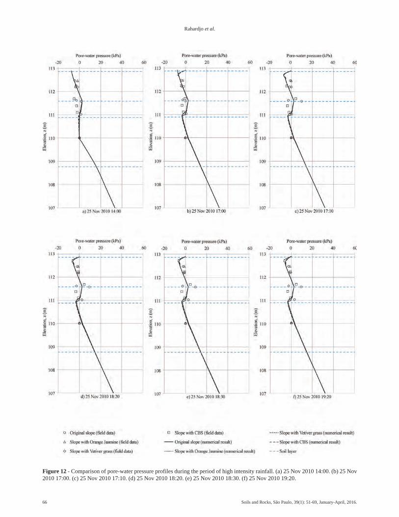
66 Soils and Rocks, São Paulo, 39(1): 51-69, January-April, 2016.
Rahardjo et al.
Figure 12 - Comparison of pore-water pressure profiles during the period of high intensity rainfall. (a) 25 Nov 2010 14:00. (b) 25 Nov2010 17:00. (c) 25 Nov 2010 17:10. (d) 25 Nov 2010 18:20. (e) 25 Nov 2010 18:30. (f) 25 Nov 2010 19:20.

ness of cover system in maintaining soil suction in theslope during rainfall.
5.3 Slope stability analyses
Slope stability analyses were performed using Bishopsimplified method by incorporating pore-water pressures atthe periods of low and high intensity rainfall. Shear strengthparameters used in the analyses are shown in Table 7. In theanalyses for slope with Orange Jasmine and slope withVetiver grass, the shear strengths on 29 July 2010 wereused for the slope stability analyses of the period of low in-tensity rainfall whereas the shear strengths on 18 Novem-ber 2010 were used for the slope stability analyses of theperiod of high intensity rainfall.
Variations of the factor of safety (FoS) of the differ-ent slopes during the period of low intensity rainfall areshown in Fig. 13. FoS of the slopes during the period of lowintensity rainfall vary from 2.1 to 2.3. The small variationin FoS indicated that the performances of the differentslope covers in maintaining matric suction in the slope wereessentially similar.
Variations of FoS of the different slopes during theperiod of high intensity rainfall are shown in Fig. 14. FoS ofthe slopes during the period of high intensity rainfall varyfrom 2.0 to 2.1. The small variation in FoS indicated thatthe performances of the different slope covers in maintain-ing matric suction in the slope were essentially similar.
In addition to the above analyses, a stability analysiswas performed using a maximum rainfall intensity of533.2 mm/day that occurred continuously for 1 day basedon a 25-year return period. This rainfall intensity is a maxi-mum total amount of rainfall in a day of 533.2 mm thatshould be used in drainage system design in Singapore(PUB 2000). The effectiveness of the different slope coversexperiencing this rainfall intensity was investigatedthrough this analysis. The results are shown in Fig. 15.
The slopes had an initial FoS of around 2. After sub-jecting the slopes to the maximum daily rainfall, FoS ofthe slopes dropped to around 1.6. After the end of rainfall,FoS of the slopes with covers recovered faster than that ofthe original slope, indicating the effectiveness of the dif-ferent cover systems in recovering FoS of the slopes afterthe maximum daily rainfall as compared to the originalslope without cover. In addition, FoS of the slopes withslope covers were essentially similar throughout the studyperiod.
6. Conclusions
Laboratory test results show that the presence of rootincreases shear strength of soils. The increase in shearstrength is indicated by the increase in effective cohesion inboth soils with Orange Jasmine roots and with Vetivergrass roots and by the increase in �b angle in the soil with
Soils and Rocks, São Paulo, 39(1): 51-69, January-April, 2016. 67
Effectiveness of Capillary Barrier and Vegetative Slope Covers in Maintaining Soil Suction
Figure 13 - Factor of safety variation during the period of the lowintensity rainfall event on 6 July 2010.
Figure 14 - Factor of safety variation during the period of the highintensity rainfall event on 25 November 2010.
Figure 15 - Factor of safety variations during a high hypotheticalrainfall intensity of 22.2 mm/h for 24 h.

Vetiver grass roots. In addition to this, the presence of rootsresults in an increase in the saturated permeability and AEVof the soil.
Field monitoring results show that the slopes withslope covers can maintain negative pore-water pressuresbetter than the original slope without cover. The amount ofmatric suction that can be maintained by the slope coversduring the periods of low and high intensity rainfalls weresimilar for the slopes covered with Orange Jasmine, Veti-ver grass, and CBS. As a result, FoS of slopes with the dif-ferent covers were essentially similar during the low andhigh intensity rainfall periods. However, during the periodof maximum intensity rainfall the slope covers resulted in afaster recovery of FoS of the slopes as compared to the orig-inal slope without the slope cover. In addition, FoS of theslopes with slope covers were essentially similar through-out the period of maximum intensity rainfall.
AcknowledgmentThe work presented in this paper was supported by
the Housing and Development Board and Nanyang Tech-nological University, Singapore. Samwoh Pte Ltd providedthe recycled concrete aggregate used in this study.
ReferencesBrand, E.W. (1992). Slope instability in tropical areas. In:
Proc. 6th International Symposium on Landslides,Christchurch, New Zealand, pp. 2031-2051.
Fredlund, D.G. & Rahardjo, H. (1993). Soil Mechanics forUnsaturated Soils. John Wiley & Sons Inc., New York,517 p.
Fredlund, D.G. & Xing, A. (1994). Equations for the soil-water characteristic curve. Canadian GeotechnicalJournal, 31(4):521-532.
Gasmo, J.M.; Rahardjo, H. & Leong, E.C. (2000). Infiltra-tion effects on stability of a residual soil slope. Com-puters and Geotechnics, 26(2):145-165.
GEO-SLOPE International Pte. Ltd. (2007a). SEEP/WUser’s Guide for Slope Stability Analysis. Geoslope In-ternational Ltd., Calgary, Alberta, Canada, 307 p.
GEO-SLOPE International Pte. Ltd. (2007b). SLOPE/WUser’s Guide for Slope Stability Analysis. Geoslope In-ternational Ltd., Calgary, Alberta, Canada, 355 p.
Grimshaw, R.G. (1994). Vetiver grass-Its use for slope andstructure stabilization under tropical and semitropicalconditions. In: Vegetation and Slopes. Institution ofCivil Engineers, London, pp. 26-35.
Khire, M.; Benson, C. & Bosscher, P. (2000). Capillarybarriers: design variables and water balance. Journal ofGeotechnical and Geoenvironmental Engineering,ASCE, 126(8):695-708.
Krisdani, H.; Rahardjo, H. & Leong, E.C. (2008). Measure-ment of geotextilewater characteristic curve using cap-illary rise principle. Geosynthetics International,15(2):86-94.
Leong, E.C. & Rahardjo, H. (1997). A review on soil-watercharacteristic curve equations. ASCE Journal ofGeotechnical and Geoenvironmental Engineering,123(12):1106-1117.
Morel-Seytoux, H.J. (1994). Steady-state effectiveness of acapillary barrier on a sloping interface. In: Proc. 14thHydrology Days Conference, Fort Collins, pp. 5-8.
Morel-Seytoux, H.J. (1993). Dynamic perspective on thecapillary barrier effect at the interface of an upper finelayer with a lower coarse layer. In: Proc. of EngineeringHydrology, San Francisco, pp. 467-472.
Morris, C.E. & Stormont, J.C. (1997a). Capillary barriersand subtitle D covers: Estimating equivalency. Journalof Environmental Engineering, ASCE, 123(1):3-10.
Morris, C.E. & Stormont, J.C. (1997b). Closure to “Capil-lary barriers and subtitle D covers: estimating equiva-lency” by Carl E. Morris and John C. Stormont. Journalof Environmental Engineering, ASCE, 123(1):3-10.
National Research Council (1993). Vetiver Grass: A ThinGreen Line Against Erosion. National Academy Press,Washington DC, 188 p.
Pham, H.; Fredlund, D.G. & Barbour, S.L. (2005). A studyof hysteresis models for soil-water characteristic cur-ves. Canadian Geotechnical Journal, 42(6):1548-1568.
Pitts, J. (1985). An Investigation of Slope Stability on theNTU Campus, Singapore. Applied Research ProjectRPI/83. Nanyang Technological Institute, Singapore.
PUB (2000). Code of Practice on Surface Water Drainage.Public Utilities Board, Singapore, 63 pp.
Ross, B. (1990). The diversion capacity of capillary barri-ers. Water Resources Research, 26(10):2625-2629.
Steenhuis, T.S.; Parlange, J.-Y. & Kung, K.-J. (1991).Comment on “The Diversion Capacity of CapillaryBarriers” by Benjamin Ross. Water Resources Re-search, 27(8):2155-2156.
Stormont, J.C. (1996). The effectiveness of two capillarybarriers on a 10% slope. Geotechnical and GeologicalEngineering, 14(4):243-267.
Styczen, M.E. & Morgan, R.P.C. (1995). Engineering pro-perties of vegetation. In: R.P.C. Morgan and R.J.Rickson (eds) Slope Stabilization and Erosion Control.E & FN Spon, London, pp. 5-58.
Tami, D.; Rahardjo, H.; Leong, E.C. & Fredlund, D.G.(2004a). A physical model for sloping capillary barri-ers. Geotechnical Testing Journal, 27(2):173-183.
Tami, D.; Rahardjo, H.; Leong, E.-C. & Fredlund, D.G.(2004b). Design and laboratory verification of a physi-cal model of sloping capillary barrier. CanadianGeotechnical Journal, 41(5):814-830.
Tan, S.B.; Tan, S.L.; Lim, T.L. & Yang, K.S. (1987). Land-slides problems and their control in Singapore. In: Proc.9th Southeast Asian Geotechnical Conference, Bang-kok, Thailand, v. 1, pp. 25-36.
68 Soils and Rocks, São Paulo, 39(1): 51-69, January-April, 2016.
Rahardjo et al.

TenCate (2011). TenCate Polyfelt TS Nonwoven Geotex-
tiles. TenCate Geosynthetics Asia Sdn. Bhd. Selangor
Darul Ehsan, Malaysia, 8 pp.
Truoung, P. & Gawander, J.S. (1996). Back from the fu-
ture: do’s and don’ts after 50 years of Vetiver utilisation
in Fiji. Proc. First International Conference on Vetiver.
Office of the Royal Development Projects Board,
Bangkok, pp. 12-17.
Tsaparas, I.; Rahardjo, H.; Toll, D.G. & Leong, E.C.(2002). Controlling parameters for rainfall-inducedlandslides. Computers and Geotechnics, 29(1):1-27.
World Bank (1995). Vetiver Grass for Soil and Water Con-servation. Technical Paper No. 273. RG Grimshaw(ed), Washington DC, 281 p.
Yang, H.; Rahardjo, H.; Leong, E.C. & Fredlund, D.G.(2004b). A study of infiltration on three sand capillarybarriers. Canadian Geotechnical Journal, 41(4):629-643.
Soils and Rocks, São Paulo, 39(1): 51-69, January-April, 2016. 69
Effectiveness of Capillary Barrier and Vegetative Slope Covers in Maintaining Soil Suction


Influence of Poisson’s Ratio on the Stress vs. SettlementBehavior of Shallow Foundations in Unsaturated
Fine-Grained SoilsW.T. Oh, S.K. Vanapalli
Abstract. Poisson’s ratio is typically assumed to be constant for both saturated and unsaturated soils. However, theback-calculated Poisson’s ratio using the relationship between elastic and shear modulus (i.e. the equation for homoge-neous, isotropic and linear elastic continuum) published in the literature showed that the Poisson’s ratio is not constant butdecreases with the degree of saturation (or increasing suction). In the present study, more focused investigations are under-taken to study the influence of Poisson’s ratio on the stress vs. settlement (SVS) behaviour of shallow foundations in an un-saturated fine-grained (UFG) soil. The FEA are carried out using the software, SIGMA/W (GeoStudio 2007) to betterunderstand the SVS behavior taking account of the influence of Poisson’s ratio for different matric suction values and com-pared with the model footing tests conducted in an UFG soil. Several suggestions are made with respect to the influence ofPoisson’s ratio on the SVS behavior of shallow foundations in the UFG soils based on the results of this study.Keywords: unsaturated soil, poisson’s ratio, stress vs. settlement, shallow foundation, finite element analysis.
1. Introduction
In recent years, significant advancements were madein the area of geotechnical engineering applications extend-ing the mechanics of unsaturated soils for the shallow foun-dations (Ausilio & Conte 1999, Costa et al., 2003, Cerato &Lutenegger 2006, Oh & Vanapalli 2013a), deep founda-tions (Weaver & Grandi 2009, Vanapalli & Taylan 2012),and heave analysis (Chao et al., 2001), etc.. However, labo-ratory or field studies on the unsaturated soils are time-consuming, cumbersome, and require elaborate testingequipment. Due to this reason, more and more studies onthe unsaturated soils are directed to Finite Element Analy-sis (hereafter referred to as FEA), which can be attributed tothe recent advancements with respect to several semi-empi-rical or constitutive models for unsaturated soils (Geor-giadis et al., 2003, Vu & Fredlund 2006, Wejrungsikul etal., 2011, Oh & Vanapalli 2011a,b, Adem & Vanapalli2013, Gallipoli et al., 2013). In the present study, an at-tempt is made to estimate the stress vs. settlement (hereafterreferred to as SVS) behavior of a model footing (i.e. shal-low foundation) in unsaturated fine-grained (hereafter re-ferred to as UFG) soils using the FEA extending mechanicsof unsaturated soils.
The bearing capacity and settlement are two key pa-rameters in the design of shallow foundations. However, itis commonly acknowledged that the design of shallowfoundations is typically governed by settlement behaviorrather than the bearing capacity. Mohamed & Vanapalli(2006) carried out model footing (B x L = 100 mm x100 mm and 150 mm x 150 mm) tests in a sandy soil for
four different average matric suction values (i.e. 0, 2, 4 and6 kPa). Based on their experimental results, Vanapalli &Mohamed (2007) proposed a semi-empirical model to esti-mate the variation of bearing capacity of coarse-grainedsoils with respect to matric suction. However, the SVS be-haviours from the model footing test results showed that thematric suction has significant influence on not only bearingcapacity but also on the initial tangent elastic modulus, Ei.In other words, the reliable estimation of elastic settlementin unsaturated soils can be obtained by considering the vari-ation of initial tangent elastic modulus with respect tomatric suction. By extending this concept, Oh et al. (2009)proposed a semi-empirical model that can be used to esti-mate the variation of initial tangent elastic modulus with re-spect to matric suction for coarse-grained soils below shal-low foundations. This model uses two fitting parameters, �and � and the Soil-Water Characteristic Curve (hereafterreferred to as SWCC). Vanapalli & Oh (2010) extended thismodel to fine-grained soils with Plasticity Index, Ip valuesless than 16% and showed that fitting parameter, � is afunction of Ip. This model can be effectively used to esti-mate elastic settlement of unsaturated soils below shallowfoundations; however, there is limitation to identify stressranges corresponding to elastic settlement. To overcomethis disadvantage, Oh & Vanapalli (2011a) proposed twomethods to predict the variation of the SVS behavior ofshallow foundations located on the surface of coarse-grained soils. In the first method, the SVS behavior wasidealized using two straight lines, which represent elasticand perfectly plastic behaviour, respectively. These two
Soils and Rocks, São Paulo, 39(1): 71-79, January-April, 2016. 71
Won Taek Oh, Ph.D., Department of Civil Engineering, University of New Brunswick, Fredericton, Canada. e-mail: [email protected] K. Vanapalli, Ph.D., Department of Civil Engineering, University of Ottawa, Ottawa, Ontario, Canada. e-mail: [email protected] Article, no discussion.

straight lines were established extending the concepts pro-posed by Oh et al. (2009) and Vanapalli & Mohamed(2007) to predict the initial tangent modulus of subgrade re-action based on initial tangent elastic modulus and bearingcapacity with respect to matric suction, respectively. In thesecond method, the FEA was carried out also using elastic -perfectly plastic model with Mohr-Coulomb yield criterion(Chen & Zhang 1991). In the FEA, the soil profile was as-sumed to be a single layer with average matric suctionvalue (i.e. constant total and apparent cohesion and initialtangent elastic modulus). The second method (i.e. FEA) hasbeen successfully used to simulate the SVS behavior ofin-situ footing (B x L = 1 m x 1 m) load test results in unsat-urated sand (Oh & Vanapalli 2011b, 2012). The studies byOh & Vanapalli (2011b, 2012) show that the SVS behav-iour of shallow foundation in unsaturated soils can be reli-ably estimated when the FEA is carried out using the elasticmodulus function (i.e. variation of elastic modulus with re-spect to the matric suction). This is because the FEA basedon elastic - perfectly plastic model is mainly influenced bythe elastic modulus and the Poisson’s ratio, �. Oh & Vana-palli (2012) investigated the influence of the Poisson’s ratioon the SVS behavior of shallow foundation by conductingthe FEA for different � values. The estimated SVS behaviorwere relatively close to each other for the � values used inthe analysis (i.e. � = 0.1, 0.2, 0.3, 0.4 and 0.495). However,better comparison between the measured and the estimatedSVS behaviour was obtained for the � values of 0.2 and 0.3,which are more reasonable for sands.
In the present study, more focused investigations areundertaken to study the influence of Poisson’s ratio on theSVS behaviour of shallow foundations in unsaturated fine-grained soils. The FEA are performed using the SIGMA/W(GeoStudio 2007) for the model footing tests results (Oh &Vanapalli 2013b) in UFG soils. The elastic - perfectly plas-tic model was used for the FEA and the SVS behavior esti-mated taking account of the influence of suction withdifferent values of Poisson’s ratio are compared with thosefrom the model footing tests. Based on the results of thesestudies several suggestions are made with respect to the in-fluence of Poisson’s ratio on the SVS behavior for shallowfoundations in the UFG soils.
2. Model Footing test in UnsaturatedFine-Grained Soil
Oh & Vanapalli (2013b) conducted a series of modelfooting tests on a statically compacted glacial till using spe-cially designed equipment (Fig. 1). The tests were per-formed for five different average matric suction values (i.e.0, 55, 100, 160, and 205 kPa). The value of matric suction atthe center of gravity of the matric suction distribution dia-gram from 0 to 1.5B (B = width of foundation) depth regionwas considered as the average matric suction. 1.5B is thedepth in which the stress below a shallow foundation is pre-
dominant (Agarwal & Rana 1987, Vanapalli & Mohamed2007, Oh et al., 2009, Oh & Vanapalli 2011a,b). The matricsuction distribution diagrams with depth for different aver-age matric suction values were obtained based on theSWCC (Fig. 2) using water contents measured along withdepth. The SWCC was measured using pressure plate tech-nique. Figure 3 and Fig. 4 show the model footing test setupand the SVS behaviors for five different matric suction val-ues. The bearing capacity values were determined using agraphical method (i.e. stress corresponding to the intersec-tion of elastic and plastic line on the SVS behavior).
3. Finite Element AnalysisOh & Vanapalli (2011) suggested that the FEA can be
effectively used to simulate the SVS behavior of shallowfoundations on unsaturated soils using an elastic - perfectlyplastic model with the Mohr-Coulomb yield criterion. Inthe present study, commercial FEA software, SIGMA/W(GeoStudio 2007) is used to simulate the SVS of the model
72 Soils and Rocks, São Paulo, 39(1): 71-79, January-April, 2016.
Oh & Vanapalli
Figure 1 - Equipments used in the study for conducting modelfooting tests (Oh & Vanapalli, 2013b).
Figure 2 - Soil-water characteristic curve measured using pres-sure plate technique (modified after Oh & Vanapalli, 2013b).

footing test results by Oh & Vanapalli (2013b). The maininput parameters required for the elastic - perfectly plasticmodel are cohesion and internal friction angle, initial tan-gent elastic modulus, and Poisson’s ratio.
3.1. Cohesion and internal friction angle
Oh & Vanapalli (2013b) suggested that the bearingcapacity of unsaturated soils should be estimated consider-ing soil type and drainage condition. Based on this concept,they proposed two approaches, Modified Effective StressApproach (MESA) and Modified Total Stress Approach(MTSA) for unsaturated coarse- and fine-grained soils, re-spectively. In the case of unsaturated coarse-grained soils,(i) both the pore-air and the pore-water in soils are indrained condition during the loading stages and (ii) the gen-eral failure can be expected for relatively high densitycoarse-grained soils. In other words, the bearing capacity ofunsaturated coarse-grained soils can be reliably estimatedextending effective stress approach using effective shearstrength parameters, c’ and �’ for saturated condition (i.e.MESA, Vanapalli & Mohamed 2007).
q c u u S
u u S
ult unsat a w b
a w AVR
BC
( ) [ ' ( ) ( tan ' )
( )
� � � � �
�
1
�
BC N B Nc ctan ' ] .� � � �� 05(1)
where qult(unsat) = ultimate bearing capacity of unsaturatedsoils, (ua - uw)b = air-entry value, (ua - uw)AVR = average matricsuction value, S = degree of saturation, � = soil unit weight,BC = fitting parameter with respect to bearing capacity(BC = 1 for coarse-grained soils), B = width of footing, Nc,N� = bearing capacity factor from Terzaghi (1943) andKumbhokjar (1993), respectively, and
c
q
c
N
N
B
L� �
�
��
�
����
�
�
��
�
���
�
���
10. , � � � �
�
�
��
�
��
�
��10 0 4. .
B
L= shape factors
from Vesic (1973).
In SIGMA/W (2007), the influence of matric suctionon the cohesion is considered using Eq. 2 (Vanapalli et al.,1996). A constant value of effective internal friction angle,�’ can be used in the FEA as �’ is not influenced by matricsuction (Vanapalli et al., 1996, Wang et al., 2002, Nishi-mura et al., 2007).
c c u ua ww r
s r
� � ��
�
�
��
�
���
�
��
�
��' ( ) tan '
� �
� �� (2)
where c = total cohesion, c’, �’ = effective cohesion and in-ternal friction angle, respectively, (ua - uw) = matric suction,�w = volumetric water content, �s = saturated volumetricwater content, and �r = residual volumetric water content
On the other hand, the behavior of the UFG soils be-low footings can be interpreted using the punching shearfailure mechanism (Oloo 1994, Schnaid et al., 1995,Consoli et al., 1998, Costa et al., 2003, Rojas et al., 2007).For punching shear failure condition, the slip surfaces be-low footings are typically not extended to the ground sur-face but instead restricted to vertical planes and no heave isobserved on the surface of the soil as shown in Fig. 5. Thischaracteristic behaviour indicates that the bearing capacity
Soils and Rocks, São Paulo, 39(1): 71-79, January-April, 2016. 73
Influence of Poisson’s Ratio on the Stress vs. Settlement Behavior of Shallow Foundations in Unsaturated Fine-Grained Soils
Figure 3 - Equipment set-up for conducting model footing tests(Oh & Vanapalli, 2013b).
Figure 4 - Bearing capacity test results (modified after Oh &Vanapalli, 2013b).

of the UFG soils is governed by the compressibility of thesoil below a footing (i.e. soil A-A’-B-B’ in Fig. 5; hereafterreferred to as soil block). When the soil block, A-A’-B-B’is compressed due to the stress applied by a footing the soilaround the soil block acts as confining pressure. In otherwords, the bearing capacity of the UFG soils can be repre-sented as a function of a compressive strength of the soilblock. A reasonable assumption can be made with respectto the pore-air to be under drained condition while thepore-water is under undrained condition during the loadingstages of model footings or in-situ plate load tests in theUFG soils. This means that the pore-air is equal to atmo-spheric pressure and the water content in the soil is constantthroughout the loading stage. Among the various methodsavailable for estimating the shear strength of unsaturatedsoils, the constant water content (CW) test is regarded asthe most reasonable technique for simulating this loadingand drainage condition (Rahardjo et al., 2004; Infante Se-dano et al., 2007). The CW test is however time-consumingand needs elaborate testing equipments. Hence, the uncon-fined compressive shear strength for unsaturated fine-grained soils can be used instead of the conventional CWtest results. The use of unconfined compression test resultscan be justified based on the following facts and reasonableassumptions.(i) The drainage condition in unconfined compression tests
for unsaturated fine-grained soils is the same as theCW test (i.e. pore-air pressure is atmospheric pressureand the water content is constant throughout the test).
(ii) The shear strength increases with increasing confiningpressure for the same matric suction values for CWtest (Rahardjo et al., 2004). Therefore, the shearstrength obtained from the unconfined compressiontests typically provides conservative estimates.Based on this discussion, Oh & Vanapalli (2013b)
suggested that the bearing capacity of UFG soils can be es-timated using Eq. 3 extending the total stress approach (i.e.MTSA).
qq B
LNult unsat
u unsatun( )
( ) .��
��
�
�� � �
�
�
��
�
��
�
��2
1 0 2 sast (3)
where qult(unsat)= ultimate bearing capacity of unsaturatedfine-grained soil, qu(unsat) = unconfined compressive strengthfor unsaturated fine-grained soil, B, L = width and length offoundation, and Nunsat = bearing capacity factor Nc for theUFG soil.
3.2. Initial tangent elastic modulus
The initial tangent elastic modulus, Ei from plate load(or model footing) test can be calculated using Eq. 4(Fig. 6).
E
q
I B k I Bi w is w��
�
��
�
���
� �( )
( )1
12
2�
��
��
(4)
where Ei = initial tangent elastic modulus, � = Poisson’s ra-tio (i.e. � = 0.3 for coarse-grained soils), �q, �� = appliedstress and displacement in elastic range, respectively,kis = initial tangent subgrade reaction modulus (= ��/�q),B = width of footing, and Iw = influence factor (i.e. 0.88 forsquare plate)
In the case of FEA, the influence of � on the SVS be-havior is included as an input parameter. In addition, if theanalysis is conducted as axisymmetric condition the influ-ence of Iw on the SVS behavior can be considered by usingequivalent area. Hence, Oh & Vanapalli (2011a) proposedthe Eq. 5 to calcuated the Ei for the FEA.
EB
q
q
B
i ��
��
�
���
��
�
�
��
15
15
.
.��
�
�� �(5)
3.3. Poisson’s ratio
The elastic (E) and shear (G) modulus of soils are twokey parameters that are required in the evaluation of the im-mediate settlement and dynamic response behavior respec-tively of geotechnical structures in engineering practice. If
74 Soils and Rocks, São Paulo, 39(1): 71-79, January-April, 2016.
Oh & Vanapalli
Figure 5 - Punching shear failure mechanism in unsaturated fine-grained soils below a footing (modified after Oh & Vanapalli,2013b).
Figure 6 - Typical stress vs. settlement behavior from plate loadtest (Oh & Vanapalli, 2011).

a soil is assumed to be homogeneous, isotropic and linearelastic continuum the Poisson’s ratio can be calculated us-ing the relationship between the E and the G. The Poisson’sratio, � is typically assumed to be constant in the numericalmodelling studies of both saturated and unsaturated soils.Such an assumption is reasonable for coarse-grained soilssince the change in mean effective stress and associatedvolume change due to the wetting and drying cycles is neg-ligible. However, in the case of fine-grained soils, the dry-ing and wetting cycles contribute to significant volumechanges in soils, which results in different compressibilitycharacteristics with respect to the degree of saturation. Inother words, the mathematical relationship between the Eand the G that were originally developed for homogeneous,isotropic and linear elastic continuum may not applicablefor the E and the G values for unsaturated soils.
The Emax - Gmax, and Gmax - Mmax, and Mmax - Emax relation-ship for homogeneous, isotropic, and linear elastic contin-uum are given in Eqs. 6, 7, and 8, respectively.
E Gmax max ( )� �2 1 � (6)
G Mmax max
( )
( )�
��
1 2
2 1
��
(7)
M Emax max
( )
( )( )�
�� �
1
1 1 2
�� �
(8)
where Emax = maximum elastic modulus, Gmax = Maximumshear modulus and Mmax = maximum constraint modulus(i.e. E, G and M at small strain)
Equation 6 and Eq. 7 can be extended to Emax, Gmax, andMmax values measured for unsaturated soils as shown inEq. 9 and Eq. 10, respectively.
E Gunsat unsatmax( ) max( ) ( )� �2 1 � (9)
G Mmax max
( )
( )�
��
1 2
2 1
��
(10)
where Emax(unsat), G max(unsat), and M max(unsat) = Emax, Gmax, and Mmax
for unsaturated condition, respectivelyTo check the validity of Eq. 9 and Eq. 10, Oh &
Vanapalli (2012) reanalyzed the Emax(unsat), Gmax(unsat), andMmax(unsat) values measured with the bender element test tech-nique for different degree of saturation values (Mendoza etal., 2005, Alramahi et al., 2010).
Figure 7 shows the variation of back-calculated �with respect to degree of saturation for the data by Mendozaet al. (2005). The negative � and greater than 0.5 valueswere ignored since they are not realistic. A trend line isdrawn assuming � = 0.1 representing the relatively dry con-dition, which was also supported by Lee & Santamarina(2005). In the case of bender element test results by Men-doza et al. (2005), the Poisson’s ratio values are relativelyhigh with the values between 0.5 and 0.35 in the boundaryeffect zone, which indicates that the soil specimens wereclose to undrained condition. The Poisson’s ratio values in
the range of 0.35 and 0.1 typically fall in the transition ef-fect zone. In residual zone, the Poisson’s ratio graduallyconverges to a relatively constant value of 0.1.
Figure 8(a) and (b) show the variation of back-calcu-lated � values with respect to degree of saturation forclay-slurry pore and silt-slurry pore, respectively for thedata provided by Alramahi et al. (2010). The behaviorshown in Fig. 8(a) (i.e. clay-slurry pore) is similar to thatshown in Fig. 7(b); however, this behavior is not observedfor the silt-slurry pore specimen (i.e. Fig. 8(b)). The differ-ence in the back-calculated � values between the saturated(i.e. S = 100%) and the dry (i.e. S = 0%) conditions for clayspecimen (Mendoza et al., 2005) and clay- and silt-slurrypore specimens (Alramahi et al., 2010) are found to be 0.4,0.04, and 0.02 respectively. This fact indicates that the vari-ation of Poisson’s ratio with respect to degree of saturationis more predominant for finer soil materials.
The results in Fig. 7 and Fig. 8 indicates that the Pois-son’s ratio can be expressed as a function of degree of satu-ration (i.e. f(S); Eq. 11 and Eq. 12). Figure 7 and Fig. 8(a)also show that the variation of Poisson’s ratio with respectto degree of saturation is similar to that of SWCC. In otherwords, the SWCC can be used as a tool to estimate the vari-ation of Poisson’s ratio with respect to degree of saturation.
Soils and Rocks, São Paulo, 39(1): 71-79, January-April, 2016. 75
Influence of Poisson’s Ratio on the Stress vs. Settlement Behavior of Shallow Foundations in Unsaturated Fine-Grained Soils
Figure 7 - a) Degree of saturation versus maximum elastic andshear modulus relationship and (b) back-calculated Poisson’s ra-tio with respect to degree of saturation (data from Mendoza et al.,2005) (Oh & Vanapalli, 2012).

�* ( )max( )
max( )
��
���
�
���
� �E
Gf Sunsat
unsat21 (11)
�*(
max( ) max( )
max( ) max(
��
�
M G
M Gunsat unsat
unsat unsa
2
2 t
f S) )
( )�
���
�
���
� (12)
where �* = Poisson’s ratio of unsaturated soils, which is afunction of degree of saturation
4. Analysis Results
4.1. Soil properties boundary conditions used in theFEA
In the present study, the model footing test results inUFG soils as detailed in Section 2 are used. Hence, the FEAfor each average matric suction value was carried out usingthe half unconfined compressive strength as total cohesionfor five different � values (i.e. 0.1, 0.2, 0.3, 0.4, and 0.495).Figure 9 shows meshes along with boundary conditionsused in the analysis. Model footing was considered as a ma-terial with extremely high elastic modulus and shear
strength parameters in the FEA. Analyses were performedas axisymmetric condition. The ‘y-displacement fixed’boundary was assigned on the surface of the compactedsoils to simulate ‘no heave (i.e. punching failure mecha-nism’ as discussed in Section 3) condition.
4.2. Comparison between the measured and estimatedstress vs. settlement behaviors
Figure 10 shows the comparisons between the mea-sured SVS behaviors and those estimated using the FEA forfive different Poisson’s ratio values. Reasonable compari-sons were observed between the measured and the esti-mated SVS behaviors regardless of Poison’s ratio; howe-ver, best comparisons were achieved for low Poison’s ratiovalues (i.e. less than 0.3). This good comparison also indi-cates that the MTSA can be successfully extended to thesimulation of the SVS behavior of shallow foundations inUFG soils.
5. Summary and Conclusions
In the present study, the influence of Poisson’s ratioon the stress vs. settlement (SVS) behavior of a model foot-ing in an unsaturated fine-grained (UFG) soil is investi-gated. The conclusions obtained from the research can besummarized as below.
76 Soils and Rocks, São Paulo, 39(1): 71-79, January-April, 2016.
Oh & Vanapalli
Figure 8 - Back-calculated Poisson’s ratio with respect to degreeof saturation for (a) clay-slurry pore and (b) silt-slurry pore (datafrom Alramahi et al., 2010) Oh & Vanapalli, 2012).
Figure 9 - Meshes and boundary condition used in the FEA.

1. The stress vs. settlement behavior of a model footing canbe reliably estimated using the Finite Element Analy-sis (FEA) extending Modified Total Stress Approach(MTSA).
2. There was good comparison between the measured SVSbehaviors and those estimated using the FEA with thePoisson’s ratio values in the range of 0.1 and 0.3.
3. Poisson’s ratio is not constant, but varies with respect todegree of saturation. In other words, there is a strongrelationship between Poisson’s ratio and the SWCC.Hence, it is necessary to conduct more studies on vari-
ous types of unsaturated soils (including expansivesoils) to develop a semi-empirical model to estimatethe variation of Poisson’s ratio with respect to degreeof saturation using SWCC.
References
Adem, H.H. & Vanapalli, S.K. (2013). Constitutive model-ing approach for estimating the 1-D heave with respectto time for expansive soils. International Journal ofGeotechnical Engineering, 7(2):199-204.
Soils and Rocks, São Paulo, 39(1): 71-79, January-April, 2016. 77
Influence of Poisson’s Ratio on the Stress vs. Settlement Behavior of Shallow Foundations in Unsaturated Fine-Grained Soils
Figure 10 - Comparison between measured SVS behaviors and those estimated using the FEA for different Poisson’s ratio.

Agarwal, K.B. & Rana, M.K. (1987). Effect of ground wa-ter on settlement of footing in sand. Proc. 9th EuropeanConference on Soil Mechanics and Foundation Engi-neering, Dublin, pp. 751-754.
Alramahi, B.; Alshibli, K.A. & Fratta, D. (2010). Effect offine particle migration on the small-strain stiffness ofunsaturated soils. Journal of Geotechnical and Geoen-vironmental Engineering, 136(4):620-628.
Ausilio, E. & Conte, E. (1999). Settlement rate of founda-tions on unsaturated soils. Canadian Geotechnical Jour-nal, 36(5):940-946.
Cerato, A.B. & Lutenegger, A.J. (2006). Bearing capacityof square and circular footings on a finite layer of granu-lar soil underlain by a rigid base. Journal of Geotech-nical and Geoenvironmental Engineering,132(11):1496-1501.
Chao, K.C.; Neslon, J.D. & Overton, D.D. (2011). Factorsinfluencing design of deep foundations on expansivesoils. Proc. 5th Asia Pacific Conference on Unsaturatedsoils, Pattaya, Thailand, v. 2, pp. 829-834.
Chen, W.F. & Zhang, H. (1991). Structural plasticity: The-ory, problems, and CAE software. Springer-Verlag.
Consoli, N.C.; Schnaid, F. & Milititsky, J. (1998). Interpre-tation of plate load tests on residual soil site. Journal ofGeotechnical and Geoenvironmental Engineering,124(9):857-867.
Costa, Y.D.; Cintra, J.C. & Zornberg J.C. (2003). Influenceof matric suction on the results of plate load tests per-formed on a lateritic soil deposit. Geotechnical Testingjournal, 26(2):219-226.
Gallipoli, T.; Sanchez, M. & Sheeler, S. (2013). Rain-fall-induced differential settlements of foundations onheterogeneous unsaturated soils. Géotechnique,63(15):1346-1355.
Georgiadis, K.; Potts, D.M. & Zdravkovic, L. (2003). Theinfluence of partial soil saturation pile behaviour. Géo-technique, 53(1):11-25.
Infante Sedano, J.A.; Vanapalli, S.K. & Garga, V.K.(2007). Modified ring shear apparatus for unsaturatedsoils testing. Geotechnical Testing Journal, 30(1):1-12.
Kumbhokjar, A.S. (1993). Numerical evaluation of Terza-ghi’s N�. Journal of Geotechnical Engineering, ASCE,119(3):598-607.
Lee, J-S & Santamarina, J.C. (2005). Bender elements: Per-formance and signal interpretation. Journal of Geotech-nical and Geoenvironmental Engineering,131(9):1063-1070.
Mendoza, C.E.; Colmenares, J.E. & Merchán, V.E. (2005).Stiffness of an unsaturated compacted clayey soil atvery small strains. Proc. of Int. Symp. on Advanced Ex-perimental Unsaturated Soil Mechanics, Ternto,pp. 199-204.
Mohamed, F.M.O. & Vanapalli, S.K. (2006). Laboratoryinvestigations for the measurement of the bearing ca-pacity of an unsaturated coarse-grained soil. Proc. 59th
Canadian Geotechnical Conference, Vancouver,pp. 219-226.
Nishimura, T.; Toyota, H.; Vanapalli, S.K. & Oh, W.T.(2007). Evaluation of critical state parameters for an un-saturated soil. Proc. 60th Canadian Geotechnical con-ference, Ottawa, Ontario, pp. 1029-1036.
Oh, W.T.; Vanapalli, S.K. & Puppala, A.J. (2009). Semi-empirical model for the prediction of modulus of elas-ticity for unsaturated soils. Canadian GeotechnicalJournal, 48(6):903-914.
Oh, W.T. & Vanapalli, S.K. (2011a). Modelling the appliedvertical stress and settlement relationship of shallowfoundations in saturated and unsaturated sans. CanadianGeotechnical Journal, 48(3):425-438.
Oh, W.T. & Vanapalli, S.K. (2011b). Modelling the stressvs. displacement behavior of shallow foundations in un-saturated coarse-grained soils. Proc. 5th Int. Symp. onDeformation Characteristics of Geomaterials, Seoul,South Korea, pp. 821-828.
Oh, W.T. & Vanapalli, S.K. (2012). Modelling the settle-ment behaviour of in-situ shallow foundations in unsat-urated sands. Proc. Geo-Congress 2012, ASCE,pp. 2542-2551.
Oh, W.T. & Vanapalli, S.K. (2013a). Scale effect of plateload tests in unsaturated soils. International Journal ofGeomate, 4(2):585-594.
Oh, W.T & Vanapalli, S.K. (2013b). Interpreting the bear-ing capacity of unsaturated fine-grained soils usingmodified effective and total stress approaches. Interna-tional Journal of Geomechanics. (Accepted for publica-tion)
Oloo, S.Y.; Fredlund, D.G. & Gan, J.K-M. (1997). Bearingcapacity of unpaved roads. Canadian GeotechnicalJournal, 34(3):398-407.
Rahardjo, H.; Heng, O.B. & Leong, E.C. (2004). Shearstrength of a compacted residual soil from consolidateddrained and the constant water content tests. CanadianGeotechnical Journal, 41(3):1-16.
Rojas, J.C.; Salinas, L.M. & Seja, C. (2007). Plate-loadtests on an unsaturated lean clay. Proc. 2nd Int. Conf. onUnsaturated Soils, Weimar, pp. 445-452.
Schnaid, F.; Consoli, N.C.; Cumdani, R. & Milititsky, J.(1995). Load-settlement response of shallow founda-tions in structured unsaturated soils. Proc. 1st Int. Conf.on Unsaturated Soils, Paris, pp. 999-1004.
Terzaghi, K. (1943). Theoretical Soil Mechanics. JohnWiley and Sons, New York, 510 p.
Vanapalli, S.K.; Fredlund, D.G.; Pufahl, D.E. & Clifton,A.W. (1996). Model for the prediction of shear strengthwith respect to soil suction. Canadian GeotechnicalJournal, 33(3):379-392.
Vanapalli, S.K. & Mohamed, F.M.O. (2007). Bearing ca-pacity of model footings in unsaturated soils. Proc. Int.Conf. From Experimental Evidence towards Numerical
78 Soils and Rocks, São Paulo, 39(1): 71-79, January-April, 2016.
Oh & Vanapalli

Modeling of Unsaturated Soil, Weimar, Germany,pp. 483-493.
Vanapalli, S.K. & Oh, W.T. (2009). A model for predictingthe modulus of elasticity of unsaturated soils using thesoil-water characteristic curves. International Journal ofGeotechnical Engineering, 4(4):425-433.
Vanapalli, S.K. & Taylan, Z.N. (2012). Design of singlepile foundations using the mechanics of unsaturatedsoils. International Journal of Geomate, ConstructionMaterials and Environment, 2(1):197-204.
Vesic A.B. (1973). Analysis of ultimate loads of shallowfoundations. Journal of the Soil Mechanics and Founda-tion Division, ASCE 99(1):45-73.
Vu, H.Q. & Fredlund, D.G. (2006). Challenges to model-ling heave in expansive soils. Canadian GeotechnicalJournal, 43:1249-1272.
Wang, Q.; Pufahl, D.E. & Fredlund, D.G. (2002). A studyof critical state on an unsaturated silty soil. CanadianGeotechnical Journal, 39(1):213-218.
Weaver, T. & Grandi, O. (2009). Lateral load analysis ofdeep foundations in unsaturated soils. contemporarytopics in in situ testing, analysis, and reliability of foun-dations. Geotechnical Special Publications, 186:552-559.
Wejrungsikul, T.; Puppala, A.J.; Williammee, R.S.; Rut-tanaporamakul, Jr. P. & Hoyos, L.R. (2011). Inclinedload capacities of drilled shafts in unsaturated soil envi-ronments. Proc. 5th Asia Pacific Conference on Unsatu-rated soils, Pattaya, Thailand, v. 2, pp. 817-822.
Soils and Rocks, São Paulo, 39(1): 71-79, January-April, 2016. 79
Influence of Poisson’s Ratio on the Stress vs. Settlement Behavior of Shallow Foundations in Unsaturated Fine-Grained Soils


Statistical Assessment of Hydraulic Propertiesof Unsaturated Soils
G.F.N. Gitirana Jr., D.G. Fredlund
Abstract. The availability of statistical values for soil parameters is essential in reliability-based geotechnical design andsensitivity analysis. Unfortunately, there are few statistical studies available about unsaturated soil parameters. Theprimary objective of this paper is to present a methodology for the statistical assessment of hydraulic properties ofunsaturated soil and to present the results of a statistical study carried out using a large database of soil properties. Twofundamental unsaturated soil properties are considered; namely, the soil-water characteristic curve (SWCC) and thehydraulic conductivity function. Appropriate nonlinear functions and fitting parameters with well-defined and uniquephysical and/or geometrical meanings were adopted. The main contribution of this article is the establishment of centraltendency measures, standard deviations, and correlation coefficients for the unsaturated soil parameters, considering soildatasets grouped according to soil texture. It was determined based on the analyses results that the air-entry value, primarySWCC slope, residual SWCC slope, saturated hydraulic conductivity, and hydraulic conductivity function slope could bewell described using lognormal probability density functions. Finally, general guidelines are provided regarding thestatistical values to be adopted for the unsaturated soil properties studied.Keywords: unsaturated soils, soil-water characteristic curve, hydraulic conductivity, statistics, coefficient of variation,correlation coefficient.
1. Introduction
The analysis of unsaturated soil problems can be sig-nificantly enhanced and rationalized if the uncertainty asso-ciated with the soil properties is addressed through proba-bilistic analysis. Unfortunately, probabilistic analysesrequire the knowledge of statistical measures for the inputproperties involved. The availability of statistical data onunsaturated soil properties benefits a wide range of geo-technical and geoenvironmental problems. Unsaturated/sa-turated seepage analysis, contaminant transport, andcover/barrier design are some of the major fields that cantake advantage of statistical data on unsaturated soil prop-erties. Other areas of application also relevant are those thatinvolve thermal and hydro-mechanical problems.
The main statistical measures required in probabilis-tic analyses are the central tendency values, standard devia-tions (or coefficients of variation), and the correlation ma-trix for the input variables. Typical, representative valuesfor the coefficients of variation and correlation coefficientsare often used for the assessment of soil properties in engi-neering practice. The adoption of a range of typical valuesis often preferable because it is not feasible to test a largenumber of soil samples to characterize a particular site(Whitman, 1984; Harr, 1987; Duncan, 2000). Typical cen-tral tendency values are also useful but are usually only rec-ommended for preliminary analyses. Numerous studies canbe found in the literature suggesting typical coefficients of
variation for saturated soil parameters (see references inTable 1). Typical values for correlation coefficients andcentral tendencies can also be found for saturated soil pa-rameters. Unfortunately, there is limited number of studiespresenting statistical assessments for unsaturated soil pa-rameters.
The primary objective of this paper is to present theresults of a statistical study carried out using 186 datasets ofsoil-water characteristic curves and hydraulic conductivityfunctions. Normality, central tendency measurements, pro-perty uncertainty, and correlations coefficients were inves-tigated. The study was directed toward the establishment ofguidelines about the typical values expected for differenttextural groups.
2. Background
A review of descriptive statistics applied to geotech-nical engineering problems was presented by Ladd (1983).Unbiased estimators can be used for the mean of a randomvariable, standard deviation, correlation coefficient be-tween two random variables, and autocorrelation coeffi-cient as a function of distance. Most statistical assessmentstudies found in the geotechnical literature, such as thestudy by Ladd (1983), deal with the uncertainty of saturatedsoil parameters. The coefficient of variation, COV, is com-monly used as a measure of uncertainty (Harr, 1987). Con-trary to the standard deviation, the coefficient of variationcan often be assumed to be independent of the magnitude of
Soils and Rocks, São Paulo, 39(1): 81-95, January-April, 2016. 81
Gilson de F. N. Gitirana Jr., PhD., Escola de Engenharia Civil e Ambiental, Universidade Federal de Goias, 74605-220 Goiania, GO, Brazil. e-mail:[email protected] G. Fredlund, PhD., Golder Associates Ltd., 1721 - 8th Street East, Saskatoon, S7H 0T4 SK, Canada. e-mail: [email protected] Article, no discussion.
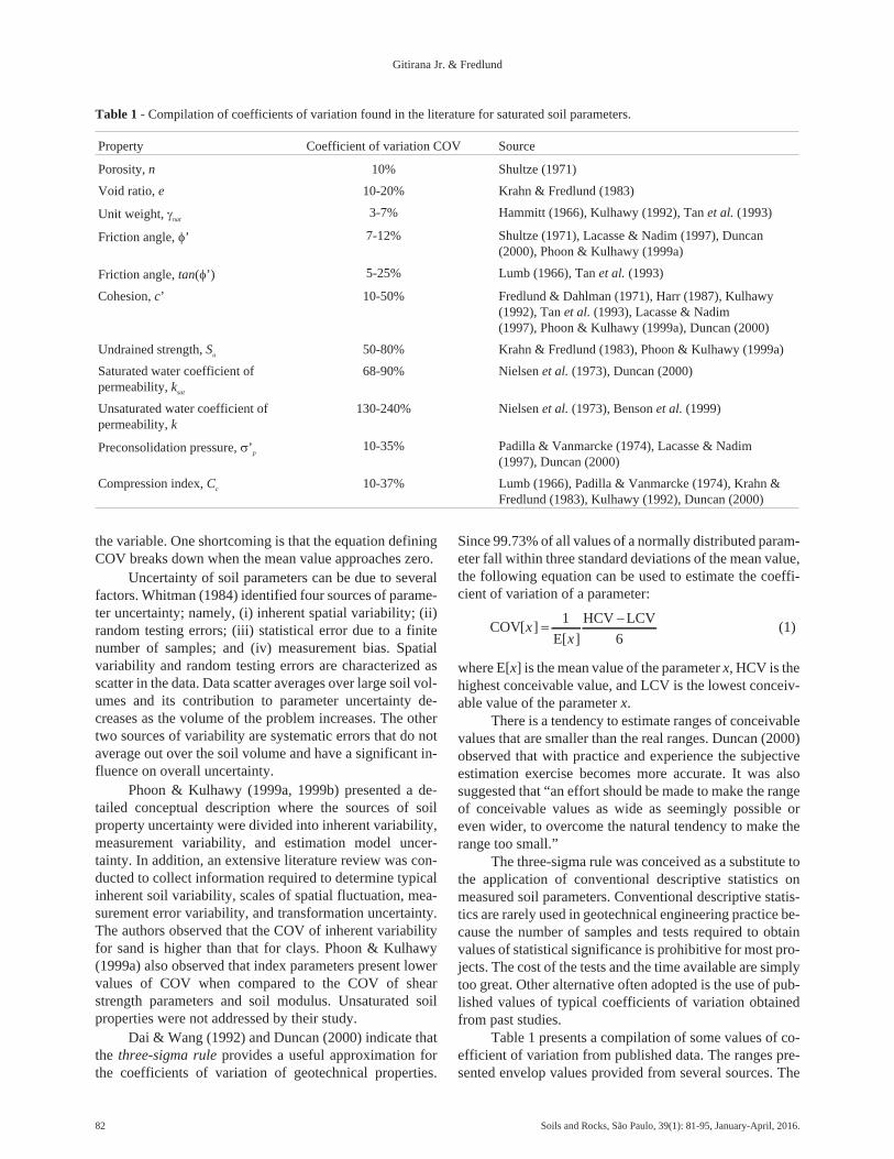
the variable. One shortcoming is that the equation definingCOV breaks down when the mean value approaches zero.
Uncertainty of soil parameters can be due to severalfactors. Whitman (1984) identified four sources of parame-ter uncertainty; namely, (i) inherent spatial variability; (ii)random testing errors; (iii) statistical error due to a finitenumber of samples; and (iv) measurement bias. Spatialvariability and random testing errors are characterized asscatter in the data. Data scatter averages over large soil vol-umes and its contribution to parameter uncertainty de-creases as the volume of the problem increases. The othertwo sources of variability are systematic errors that do notaverage out over the soil volume and have a significant in-fluence on overall uncertainty.
Phoon & Kulhawy (1999a, 1999b) presented a de-tailed conceptual description where the sources of soilproperty uncertainty were divided into inherent variability,measurement variability, and estimation model uncer-tainty. In addition, an extensive literature review was con-ducted to collect information required to determine typicalinherent soil variability, scales of spatial fluctuation, mea-surement error variability, and transformation uncertainty.The authors observed that the COV of inherent variabilityfor sand is higher than that for clays. Phoon & Kulhawy(1999a) also observed that index parameters present lowervalues of COV when compared to the COV of shearstrength parameters and soil modulus. Unsaturated soilproperties were not addressed by their study.
Dai & Wang (1992) and Duncan (2000) indicate thatthe three-sigma rule provides a useful approximation forthe coefficients of variation of geotechnical properties.
Since 99.73% of all values of a normally distributed param-eter fall within three standard deviations of the mean value,the following equation can be used to estimate the coeffi-cient of variation of a parameter:
COVE
HCV LCV
6[ ]
[ ]x
x�
�1(1)
where E[x] is the mean value of the parameter x, HCV is thehighest conceivable value, and LCV is the lowest conceiv-able value of the parameter x.
There is a tendency to estimate ranges of conceivablevalues that are smaller than the real ranges. Duncan (2000)observed that with practice and experience the subjectiveestimation exercise becomes more accurate. It was alsosuggested that “an effort should be made to make the rangeof conceivable values as wide as seemingly possible oreven wider, to overcome the natural tendency to make therange too small.”
The three-sigma rule was conceived as a substitute tothe application of conventional descriptive statistics onmeasured soil parameters. Conventional descriptive statis-tics are rarely used in geotechnical engineering practice be-cause the number of samples and tests required to obtainvalues of statistical significance is prohibitive for most pro-jects. The cost of the tests and the time available are simplytoo great. Other alternative often adopted is the use of pub-lished values of typical coefficients of variation obtainedfrom past studies.
Table 1 presents a compilation of some values of co-efficient of variation from published data. The ranges pre-sented envelop values provided from several sources. The
82 Soils and Rocks, São Paulo, 39(1): 81-95, January-April, 2016.
Gitirana Jr. & Fredlund
Table 1 - Compilation of coefficients of variation found in the literature for saturated soil parameters.
Property Coefficient of variation COV Source
Porosity, n 10% Shultze (1971)
Void ratio, e 10-20% Krahn & Fredlund (1983)
Unit weight, �nat3-7% Hammitt (1966), Kulhawy (1992), Tan et al. (1993)
Friction angle, �’ 7-12% Shultze (1971), Lacasse & Nadim (1997), Duncan(2000), Phoon & Kulhawy (1999a)
Friction angle, tan(�’) 5-25% Lumb (1966), Tan et al. (1993)
Cohesion, c’ 10-50% Fredlund & Dahlman (1971), Harr (1987), Kulhawy(1992), Tan et al. (1993), Lacasse & Nadim(1997), Phoon & Kulhawy (1999a), Duncan (2000)
Undrained strength, Su 50-80% Krahn & Fredlund (1983), Phoon & Kulhawy (1999a)
Saturated water coefficient ofpermeability, ksat
68-90% Nielsen et al. (1973), Duncan (2000)
Unsaturated water coefficient ofpermeability, k
130-240% Nielsen et al. (1973), Benson et al. (1999)
Preconsolidation pressure, �’p10-35% Padilla & Vanmarcke (1974), Lacasse & Nadim
(1997), Duncan (2000)
Compression index, Cc 10-37% Lumb (1966), Padilla & Vanmarcke (1974), Krahn &Fredlund (1983), Kulhawy (1992), Duncan (2000)

information available in the literature enables the applica-tion of reliability-based design into geotechnical practice. Itis interesting to note that cohesion, undrained strength andpermeability present considerably higher COVs. The COVof porosity and void ratio found in the literature are of par-ticular interest to the present study, since the range of pub-lished values can be compared with the value presentedherein.
Unsaturated soil properties are generally defined asnonlinear functions of the stress state variables. The nonlin-ear characteristics of such soil properties require a some-what more elaborate procedure for statistical assessmentthan that adopted for saturated soil properties. Confidencebands are often used in the statistical characterization offunctions (Bates & Watts, 1988). This was the approachused in the statistical characterization of the SWCC byMishra et al. (1989) and Zapata et al. (2000). Both authorswere able to establish typical ranges of variability expectedfor SWCCs. Unfortunately, such an approach is not conve-nient for reliability analysis. Reliability analyses can bemore easily undertaken if property variability is character-ized in terms of the variability of a finite and relativelysmall number of curve parameters. A small number of au-thors, such as Meyer et al. (1997), Rawls et al. (1998),Faulkner et al. (2003) and Phoon et al. (2010), have pre-sented statistical and probabilistic studies regarding someof the hydraulic properties of unsaturated soils. Unfortu-nately, these studies are based on specific fitting functionswhose parameters have little or no physical meaning andare not independently related to individual shape featuresof the unsaturated soil property functions.
3. Methodology for the Statistical Assessmentof Unsaturated Soil Properties
The statistical assessment of unsaturated soil proper-ties requires the establishment of an appropriate methodol-ogy regarding the selection of data and analysis procedure.This section presents the criteria established for data selec-tion and data grouping, the fitting equation that have beenused in this study, and the fitting procedure adopted.
3.1. Soil properties studied and criteria for selection ofdata records
The properties studied in this paper are for the soil-water characteristic curve, SWCC, and the hydraulic con-ductivity function. Data records were sampled from a soilsdatabase (SoilVision Systems, 2005). Only drying curveswere used in the present study, as those are the most com-monly measured and found in the literature.
Other unsaturated soil properties such as the vaporconductivity, thermal properties, and shear strength werenot analyzed in this paper due to the limited availability ofdata at the present time. However, these unsaturated soilproperties can be visualized as variables dependent on thesoil-water characteristic curve. There are numerous predic-
tive models available based on the SWCC. Consequently,the statistical study presented herein for the SWCC be-comes useful for the assessment of other unsaturated soilproperties. A complete statistical assessment of all unsatu-rated soil properties would also require studies on the un-certainties associated with the predictive models.
The term hydraulic conductivity function is usedherein to denote the relationship between the hydraulicconductivity and soil suction. The hydraulic conductivityfunction can also be treated as a property dependent on theSWCC. Huang et al. (1998) presents a review of several hy-draulic conductivity prediction methods. However, the rel-atively large amount of directly measured hydraulic con-ductivity data available provided an opportunity for theindependent analysis presented in this study.
A total of 186 soil records were sampled from theSoilVision database. The number of sampled records waslimited by the number of available “complete” soil records.To be considered “complete”, a soil record was required tohave a grain-size distribution, the soil porosity, n, the dry-ing soil-water characteristic curve, the saturated hydraulicconductivity, and the hydraulic conductivity function. Theporosity data provided an indication of total water storage.The grain-size distribution was required for the classifica-tion of each soil sample and grouping the soil data with re-spect to texture.
3.2. Fitting equations and corresponding soil parame-ters
The soil-water characteristic curve and the hydraulicconductivity function can be described using various equa-tions (Fredlund and Xing 1994) whose soil parameters canbe treated as best-fit parameters obtained using a nonlinearfitting algorithm. Unfortunately, unsaturated soil propertyfunctions have often been defined using functions whosefitting-parameters have limited physical significance andare somewhat interrelated. For instance, for most SWCCequations it is possible to obtain similar fitting with com-pletely different sets of parameters (Gitirana Jr. &Fredlund, 2004). In other words, the set of best-fit parame-ters do not appear to be unique. Consequently, it becomesdifficult to perform a meaningful statistical analysis onsuch parameters. In order to overcome these difficulties, itis suggested herein that it is better to use soil property func-tions defined by mathematically independent and prefera-bly meaningful soil parameters.
3.2.1. Soil-water characteristic curve equation
The soil-water characteristic curve datasets were fit-ted using the unimodal equations proposed by Gitirana Jr.& Fredlund (2004). Two equations were used herein;namely, the unimodal equation with two bending pointsand the unimodal equation with one bending point. Theunimodal equation with two bending points can be writtenas follows:
Soils and Rocks, São Paulo, 39(1): 81-95, January-April, 2016. 83
Statistical Assessment of Hydraulic Properties of Unsaturated Soils

SS S
S
b res
d�
�
��
�
�
�1 22
1�
� �
(2)
S
r
ri
i i
ia
i i
i�
��
�
�
�� � �
�tan ( ) ln
tan( )
t�
�
�
�
1
11
12
2 2
an
tan
ln( tan
2
2 2
2 22 2 2
1
1
�
�
�
�
�
i
i i
i
ia
i i
r
ra r
��
�
�
� �
� )
tan1 2��
� i
iaS
(3)
where i = 1, 2; �i = -(�i-1 + �i)/2; ri = tan ((�i-1 - �i)/2); �0 = 0;�i = arctan [(Sa
i - Sa
i+1) / (ln(�a
i+1/�a
i))]; S1
a = 1; S2
a = Sres;S3
a = 0; �1
a = �b; �2
a = �res; �3
a = 106; d = 2exp(1/ln(�res/�b));� = soil suction; and a is a parameter controlling the curvesharpness at the two bending points.
The unimodal equation with one bending point can beobtained directly from Eq. 3, making S = S1, �1 = -�/2,r1 = tan (�/2), and � = arctan [1/(ln(106/�b))].
According to Eq. 2, a SWCC with two bending pointscan be defined using four parameters; namely, �b = air-entry value; �res = residual suction; Sres = residual degree ofsaturation; and the sharpness parameter, a. These four pa-rameters correspond to the number of shape features of atypical SWCC (see Fig. 1). Figure 1 also shows that twoshape features define a SWCC with one bending point;namely, �b and a. Each one of these soil parameters have aphysical meaning (Gitirana Jr. & Fredlund, 2004).
Other SWCC parameters are defined in Fig. 1;namely, �d, the primary drainage slope; and �res, the residualdrainage slope. The primary and residual drainage slopescan be calculated as follows:
��
�
dres
res
b
S�
�
�
�
�
1
10log
(4)
�
�
resres
res
S�
�
�
� log
, ,10
1 000 000(5)
The primary drainage slope, �d, is influenced by thedistribution of the pore-sizes. Uniform pore-size distribu-tions result in steeper primary drainage slopes.
Four parameters should be used to describe theSWCC because the curve has four distinct shape features.The use of a number of parameters lower than four wouldimpose restrictions to the SWCC shape. The set of parame-ters �b, �d, �res, and a was deemed to be appropriate for thisstudy. For instance, difficulties in probabilistic analyseswould arise for estimate points (or random realizations) of�b greater than �res, a combination of parameters that isphysically inadmissible. The use of constraints to prevent�b > �res is mathematically cumbersome and, as a result, �res
and Sres were replaced by �d and �res.
Most sampled SWCC datasets show curves with twobending points (e.g., curve 2 in Fig. 1). However, most claysoils have SWCCs with only one bending point and do notpresent a distinguishable residual point (e.g., curve 1 inFig. 1). As a result, all clay datasets were fitted using theunimodal equation with one bending point, while other soiltypes where fitted using an equation with two-bendingpoints.
Gitirana Jr. & Fredlund (2004) show that the parame-ter a slightly improves the fitting capabilities of the equa-tion. However, the physical meaning of a is not as clear andas significant as the physical meaning of the other threeSWCC parameters. Therefore, fixed values were adoptedfor a, based on the observation that a good fit could be ob-tained for the absolute majority of data when using the cho-sen values. A value of a equals to 0.075 was selected for allSands, 0.050 was selected for Loams, and 0.025 was se-lected for Clays.
3.2.2. Hydraulic conductivity function
The hydraulic conductivity function datasets were fit-ted using a bi-linear function on a log vs. log plot (seeFig. 2). The bi-linear shape was found to fit reasonably wellmost experimental curves. The first portion of the curve isdefined using a constant value equal to the saturated hy-draulic conductivity, ksat. The value of ksat was not treated asa fitting parameter but as an independently measured value.The second portion of the curve was assumed to be definedby a constant slope, �. The following bi-linear equationwas used (Brooks & Corey, 1964):
k k
k k
sat bk
satbk
n
bk
� �
��
��
�
�� �
for
for
� �
�
�� �
(6)
84 Soils and Rocks, São Paulo, 39(1): 81-95, January-April, 2016.
Gitirana Jr. & Fredlund
Figure 1 - Idealization of a unimodal soil-water characteristiccurve with one and two bending points.

where k = hydraulic conductivity; ksat = saturated hydraulicconductivity; �bk = break point of the hydraulic conductiv-ity function; � = slope of the hydraulic conductivity func-tion.
In theory, the break point, �bk, corresponds to theair-entry value, �b. However, it was found that the air-entryvalue obtained from the SWCC fitting does not alwaysmatch the break point observed in the hydraulic conductiv-ity function. The use of �bk equal to �b would compromisethe fitting capability of Eq. 6. As a result, the fitting of thehydraulic conductivity function was made independently ofthe soil-water characteristic curve fit (i.e., the air-entryvalue from the SWCC was not used for the hydraulic con-ductivity function).
3.3. Fitting procedure and statistical representation ofunsaturated soil property functions
The following soil parameters were statistically as-sessed, in order to completely define the SWCC and hy-draulic conductivity function: �b, �d, �res, ksat, �bk, and �. Thedata records sampled from the SoilVision database werefirst imported into a spreadsheet. The fitting of the SWCCsand hydraulic conductivity functions was performed byminimizing the sum of the squared residuals between theexperimental data and the fitting curve. The nonlinear mini-mization solver available in MS Excel© was utilized. Thenonlinear fitting application appeared to perform well pro-vided that the initial guess was sufficiently close to the finalbest-fit parameter. Other minimization techniques are avai-lable and some of these have been described by Fredlund &Xing (1994).
Figures 1 and 2 illustrate the manner in which thesoil-water characteristic curve and the hydraulic conductiv-ity function can be statistically described based on the sta-tistical characterization of the soil parameters �b, �d, �res,ksat, �bk, and �. Each soil parameter was considered as a ran-dom variable with a frequency distribution characterizedbased on statistical descriptive measures, as traditionallydone for other soil properties.
3.4. Soil grouping based on the USDA textural classifi-cation system
The 186 soil records sampled from the SoilVision da-tabase are diverse soils with distinct characteristics.Ideally, the statistical assessment of individual “soilgroups” is preferable (Fredlund & Dahlman, 1971) eventhough the definition of the term “soil group” is not totallyprecise. To address that concern, the sampled records weregrouped according to their textural characteristics. The sep-aration of soil types is an attempt to group soils with similarengineering behavior, even though soil behavior dependson many other characteristics.
Two of the commonly used soil classification systemsare the USDA system (Soil Survey Staff, 1975) and theUnified Soil Classification System, USCS, (ASTM, 1993).The USCS system is generally preferred in geotechnicalengineering. However, the number of “complete” recordsin the SoilVision database where Atterberg limits are pre-sented is small. As a result, the USDA system has beenadopted herein.
Figure 3 presents the textural diagram used in theUSDA soil classification system (Soil Survey Staff, 1975)along with the textural characteristics of the data recordssampled. The percentages of sand, silt and clay plotted inFig. 3 were defined using the following particle size, x, in-tervals: Clay: x < 0.002 mm; Silt: 0.002 � x < 0.05 mm;Sand: 0.05 � x < 2 mm; and Coarse material:2 � x < 300 mm.
Three main groups are identified in Fig. 3; namely,sands (Sa), loams (L), and clays (C). The silt and silty frac-tions (Si) are placed within the loam fraction. The numberof sampled records pertaining to each soil group is 62, mak-ing a total of 186 sampled records. Each of the three mainsoil groups is subdivided into a number of subgroups (Sa,
Soils and Rocks, São Paulo, 39(1): 81-95, January-April, 2016. 85
Statistical Assessment of Hydraulic Properties of Unsaturated Soils
Figure 2 - Idealization of a hydraulic conductivity function.
Figure 3 - Sampled soil records classified according to the USDAclassification system.

L-Sa, Sa-L, Sa-C-L, L, Si-L, Si, C-L, Si-C-L, Sa-C, Si-C,and C).
4. Results and Discussion of Normality Tests
Normality tests were performed on the soil parame-ters and on the natural logarithm of most soil parameters inorder to determine whether normal or lognormal densityfunctions reasonably represent each unsaturated soil pa-rameter. Normality tests were performed with the aid ofMinitab 13 (Minitab Inc., 2000). Minitab has three hypoth-esis tests available for testing normality; namely, Ander-son-Darling test; Ryan-Joiner test; and Kolmogorov-Smir-nov test. D’Augostino & Stevens (1986) present detaileddescriptions and comparisons of these tests for normality.The Anderson-Darling test has relatively superior powerfor detecting non-normality and was selected. The null hy-pothesis for the Anderson-Darling test is “H0: data follow anormal distribution”. The results of the normality tests arepresented in terms of p-values. P-values represent the prob-ability of making a type 1 error, which is “rejecting the nullhypothesis when it is true.” A cut-off value often used was5%, which means “reject the null hypothesis when thep-value is less than 5%” (D’Augostino and Stevens 1986).
Sampled records were grouped according to theUSDA classification system, as presented in Fig. 3. For thenormality tests the analyses were carried out followingthree distinct procedures: a) considering all the sampled re-cords as one single group; b) assembling the data using thethree main groups of soils (i.e., Sa, L, and C); and c) assem-bling the data using the smaller soils subgroups indicated inFig. 3. The soil subgroups Si, C-L, Si-C-L, and Sa-C couldnot be analyzed because of the relatively small number ofsample records in those subgroups.
Figure 4 present the results of the normality tests interms of p-values. Dashed lines indicate the threshold of5%, below which normality is unlikely. Figure 4 shows thatmost parameters and soil groups deviate to some extentfrom a normal distribution. This is particularly true for �b,�d, �res, ksat, �bk, and �. When the logarithm of �b, �d, �res, ksat,�bk, and � were tested the parameters were closer to beingnormally distributed (i.e., larger p-values). Based on the re-sults presented in Fig. 4, it was concluded that the parame-ters �b, �d, �res, ksat, �bk, and � can be considered log nor-mally distributed while n is reasonably described using anormal distribution.
The effect to the normality tests of grouping soil datainto textural classes can be clearly observed in Fig. 4. Noneof the parameters were found to be normally or log nor-mally distributed when all sampled records were analyzedas a single soil. The more detailed soil textural classifica-tion (Fig. 4b) appears to produce parameter distributionsthat are better described by normal and lognormal distribu-tions.
5. Results and Discussion of DescriptiveStatistics Analysis
Tables 2 and 3 present descriptive statistical parame-ters obtained for the three main soil groups; namely, sands(Sa), loams (L), and clays (C). The minimum and maximumvalues are presented along with measures of central ten-dency and the standard deviation. Three measures of cen-tral tendency were calculated; namely, the median, themean, and the global best-fit parameters. The global best-fitparameters were obtained by assembling in the same plotall the datasets pertaining to a given soil group.
86 Soils and Rocks, São Paulo, 39(1): 81-95, January-April, 2016.
Gitirana Jr. & Fredlund
Figure 4 - Normality tests: p-values for all soil parameters considering (a) the three main soil groups and (b) all soil subgroups.

Table 4 presents a summary of the coefficients ofvariation, COV, obtained from the statistical analyses.Two main measures are usually considered in the quanti-fication of uncertainty; namely, the standard deviation,
SD, and the coefficient of variation. The standard devia-tion of a random variable is strongly influenced by themean values and depends on the units of the variable. Thecoefficient of variation tends to offer a means of normal-
Soils and Rocks, São Paulo, 39(1): 81-95, January-April, 2016. 87
Statistical Assessment of Hydraulic Properties of Unsaturated Soils
Table 2 - Descriptive statistics for unsaturated soils properties (a = 0.075 for sands, 0.050 for loams, and 0.025 for clays).
Group Measure n �b (kPa) �d �resksat (m/s) �bk (kPa) �
Sands Min 0.297 0.183 0.405 0.019 3.8 x 110-7 0.100 1.288
Max 0.570 12.00 4.228 0.126 3.50 x 10⁻⁴ 7.239 10.500
Median 0.409 2.438 1.178 0.044 1.82 x 10⁻⁵ 1.585 3.484
Mean 0.410 2.937 1.446 0.047 3.88 x 10⁻⁵ 1.874 4.037
Global best-fit — 1.64 0.844 0.049 7.06 x 10⁻⁶ 1.550 3.107
Std. Dev. 0.055 2.050 0.880 0.021 6.34 x 10⁻⁵ 1.582 2.141
Loams Min 0.378 0.054 0.177 0.038 3.49 x 10⁻⁸ 0.040 1.027
Max 0.715 40.000 2.471 0.144 1.33 x 10⁻⁴ 10.000 7.657
Median 0.471 2.697 0.371 0.087 3.23 x 10⁻⁶ 1.000 2.057
Mean 0.501 4.398 0.633 0.090 1.42 x 10⁻⁵ 2.032 2.792
Global best-fit — 1.351 0.334 0.103 3.14 x 10⁻⁶ 0.830 1.954
Std. Dev. 0.085 6.190 0.571 0.025 2.50 x 10⁻⁵ 2.261 1.624
Clays Min 0.351 0.500 — — 5.42 x 10⁻¹⁰ 0.030 1.094
Max 0.790 4932.4 — — 5.88 x 10⁻⁶ 6.000 4.933
Median 0.544 2.11 — — 1.17 x 10⁻⁷ 2.078 2.000
Mean 0.534 91.4 — — 5.51 x 10⁻⁷ 2.363 2.095
Global best-fit — 2.505 — — 1.39 x 10⁻⁶ 0.179 1.571
Std. Dev. 0.100 626.1 — — 1.16 x 10⁻⁶ 1.614 0.791
Table 3 - Descriptive statistics for the natural logarithm of unsaturated soil properties (a = 0.075 for sands, 0.050 for loams, and 0.025for clays).
Group Measure ln(�b) ln(kPa) ln(�d) ln(�res) ln(ksat) ln(m/s) ln(�bk) ln(kPa) ln(�)
Sands Min -1.701 -0.904 -3.968 -14.78 -2.303 0.253
Max 2.485 1.442 -2.068 -7.96 1.979 2.351
Median 0.891 0.163 -3.119 -10.91 0.461 1.248
Mean 0.856 0.198 -3.141 -11.34 0.119 1.268
Std. Dev. 0.733 0.592 0.430 1.736 1.180 0.506
Loams Min -2.914 -1.734 -3.270 -17.17 -3.219 0.027
Max 3.689 0.905 -1.940 -8.92 2.303 2.036
Median 0.992 -0.991 -2.446 -12.64 0.000 0.721
Mean 0.927 -0.737 -2.445 -12.58 -0.047 0.895
Std. Dev. 1.090 0.689 0.291 1.870 1.391 0.492
Clays Min -1.049 — — -21.34 -3.507 0.089
Max 8.504 — — -12.04 1.792 1.596
Median 0.743 — — -15.96 0.731 0.693
Mean 0.999 — — -16.03 0.527 0.682
Std. Dev. 2.064 — — 2.053 0.992 0.331

izing the standard variation with respect to the meanvalue. The coefficient of variation is unitless and hasbeen traditionally used for characterizing geotechnicalparameter uncertainty.
It was shown in the previous section that the parame-ters �b, �d, �res, ksat, �bk, and � can be better analyzed in termsof natural logarithm. Therefore, values of COV are pre-sented for the natural logarithms of all soil parameters, withexception of porosity, which was not considered log nor-mally distributed. The coefficients of variations for n,ln(�b), ln(�d), ln(�res), ln(ksat), ln(�bk), and ln(�) are pre-sented for each USDA group. Some neighboring groupswith a reduced number of records where joined, as indi-cated. The data summarized in Tables 2-4 will be discussedin the following sections.
5.1. Porosity
The mean value of porosity, n, is 0.410 for sands,0.501 for loams, and 0.534 for clays. The median values ob-tained do not differ considerably from the mean. Both themean and median values appear to provide a reasonablemeasure of the central tendency for porosity. The mini-mum, maximum, median, and mean porosities increase forfiner-grained soils, as expected.
The standard deviations and coefficients of variationincrease for finer-grained soils. The coefficients of varia-tion of porosity were 13.5% for sands, 17.1% for loams,and 18.7% for clays. The values previously reported in theliterature show COVs for porosity varying from 10% to20%. The results obtained herein suggest that the variabil-ity of the soil records studied may be slightly higher thanthat of soil records obtained from a single location or soilformation.
Figure 5 presents a plot of mean values of porosity vs.the computed coefficients of variation. Each data point cor-responds to a distinct soil group gathered from the sampled
soil records. The two lines surrounding the data pointscorrespond to constant values of standard deviation, as in-dicated. One outlier was ignored. The data points plotted inFig. 5 indicate that the COV for porosity show little varia-tion with the mean value, as is often assumed. Althoughsome of the results presented for porosity may appear obvi-ous, the availability of statistical data in the literature al-lows comparisons that serve as verifications of the validityof the results obtained.
5.2. Air-entry value
The mean air-entry value was 2.9 kPa for sands, 4.4kPa for loams, and 91.4 kPa for clays. The median values of�b are considerably lower than the mean values, indicatingpositive skewness in the frequency distribution. However,the mean and median values of ln(�b) are in reasonableagreement. This observation supports previous observa-tions indicating the log normality of �b.
The global best-fit values of �b appear to be in pooragreement with the mean values of �b and in better agree-
88 Soils and Rocks, São Paulo, 39(1): 81-95, January-April, 2016.
Gitirana Jr. & Fredlund
Table 4 - Coefficients of variation for unsaturated soil properties.
Group Sub-group Records n ln(�b) ln(�d) ln(�res) ln(ksat) ln(�bk) ln(�)
All —- 186 20.2 151.6 294.4 18.1 20.6 608.8 53.7
Sands All 62 13.5 85.6 299.3 13.7 15.3 988.7 39.9
Sa 53 12.7 92.1 279.9 13.9 15.4 5439.9 43.0
L-Sa 9 13.7 53.2 655.6 8.5 15.3 111.3 14.4
Loams All 62 17.1 117.6 93.5 11.9 14.9 2962.5 55.0
Sa-L 15 11.3 105.5 74.5 10.2 13.6 539.3 60.3
Si-L 27 13.5 74.3 133.2 11.4 15.7 365.4 57.7
L 12 18.0 684.0 49.6 8.9 13.5 177.2 33.3
Sa-C-L & C-L 8 16.3 149.2 101.0 12.2 14.3 937.3 55.3
Clays All 62 18.7 206.6 — — 12.8 188.2 48.6
Si-C 22 26.3 125.5 — — 10.4 76.5 52.2
Sa-C & C 40 13.4 295.2 — — 13.3 369.2 44.7
Figure 5 - Mean vs. the coefficient of variation of the soil poros-ity, n.

ment with the median values of �b. The best-fit air-entryvalue is also in better agreement with the exponential of themean values of ln(�b). In other words, the mean values ofln(�b) appear to be the best measurement of central ten-dency associated with �b. The data for the air-entry valueobtained from the hydraulic conductivity function lead tothe same findings
The maximum and mean air-entry values increasedfor finer grained soils, as expected. The minimum and me-dian values do not appear to show the same increasingtrend. It appears that there are some factors other than therelationship between pore-size distribution and texture thatinfluence the air-entry value. Soil structure, for instance,would appear to have a particularly important effect in theair-entry value of clay soils. Therefore, the values of �b ofclay soils can vary over a relatively large range and not al-ways be higher than those of sand and loam soils.
Figure 6 presents a comparison of �bk and �b. In the-ory, the values of �bk should be similar to the values of �b.This tendency is in part confirmed by Fig. 6, with numerousdata points near the 1:1 line. However, dispersion is ob-served and the values of �bk tend to be lower than the valuesof �b. This trend may be expected for soils that undergosubstantial volume changes. Volume changes may cause adecrease in the hydraulic conductivity (Huang et al., 1998).Consequently, a false break point in the hydraulic conduc-tivity function may appear at a value of soil suction slightlybelow the value of �b obtained from the SWCC.
The coefficients of variation obtained for the naturallogarithm of the air entry values obtained from the SWCC,ln(�b), were 85.6% for sands, 117.6% for loams, and206.6% for clays. The coefficients of variation of the air en-try values measured on the permeability functions, ln(�bk),seem unreasonably high. The COV of ln(�bk) is 989% forsands, 2962% for loams, and 188.2% for clays. The highvalues of COV of ln(�b) and remarkably high values ofCOV of ln(�bk) are due to fact that some of the mean valuesof ln(�b) and ln(�bk) are significantly close to 0 ln(kPa). The
values of COV are highly sensitive to small changes in themean value when the mean value is between -1 and 1ln(kPa) and close to 0 ln(kPa). The sensitivity of COV tosmall mean values becomes obvious by examining itsmathematical definition.
Figure 7 presents a plot of absolute values for themean ln(�b) and ln(�bk) vs. the computed COVs. Each datapoint corresponds to a distinct soil group gathered from thesampled soil records. The two lines surrounding the datapoints correspond to constant values of SD equal to 0.8ln(kPa) and 2.1 ln(kPa). Figure 7 shows that most datapoints are located between COV values of 75% and 125%.However, when the mean values of ln(�b) and ln(�bk) fallbetween -0.5 and 0.5 ln(kPa) and approach 0 ln(kPa), sig-nificantly higher values of COV are obtained.
The coefficients of variation for ln(�b) and ln(�bk)show a clear trend with soil texture. The values of COV ofln(�b) and ln(�bk) increase for fine-grained soils. This resultis anticipated since sands are known to have air entry valuesvarying over a smaller range of soil suctions while loamsand clays have air-entry values varying over a wider range.
In summary, the results obtained herein suggest thatCOV values between 75% and 125% can be adopted incases where the mean values of ln(�b) or ln(�bk) are notwithin the -0.5 to 0.5 ln(kPa) range. When the mean valuesof ln(�b) or ln(�bk) are within the -0.5 to 0.5 ln(kPa) range,the COV values should be abandoned and the parameteruncertainty should be defined using a standard deviationsbetween 0.8 and 2.1 ln(kPa).
5.3. Primary drainage slope
The mean values obtained for the primary drainageslope, �d, were 1.446 for sands and 0.633 for loams. Pri-mary drainage slope values for the SWCC of clay soils arenot reported, since those soils were described using two pa-rameters, �b and a. As observer for the air-entry value, themean values of �d for sands and loams disagreed with themedian values, indicating non symmetric frequency distri-
Soils and Rocks, São Paulo, 39(1): 81-95, January-April, 2016. 89
Statistical Assessment of Hydraulic Properties of Unsaturated Soils
Figure 6 - Air-entry values obtained by best-fit of the soil-watercharacteristic curves and the hydraulic conductivity functions.
Figure 7 - Mean vs. the coefficient of variation of the natural loga-rithm of air-entry value obtained from the SWCC and from the kfunction, ln(�b) and ln(�bk), ln(kPa).

butions. The closer agreement between the mean and me-dian values of ln(�d) corroborates previous observationsindicating the log normality of �d. It can also be observedthat the values of �d for sands are higher than those ofloams, as expected. Loam soils tend to have broader pore-size distributions than sands as reflected in the grain-sizedistributions.
The variability of the primary drainage slope was ana-lyzed in the same manner as the previous parameters. Thecoefficient of variation of ln(�d) was 299.3% for sands and93.5% for loams. The COV of ln(�d) of loams is signifi-cantly lower than that of sands. This result does not reflectthe wider grain-size distribution for loams and the narrowervariation in grain-size distribution for sands. In fact, the re-sults once again are influenced by low mean values of ln(�d)that approach zero. Figure 8 presents a plot of mean valuesof ln(�d) vs. the computed COVs. The two lines plotted cor-respond to constant values of SD that encompass all thedata points. The loam data points are closer to the maxi-mum standard deviation line.
The results obtained herein suggest that a COV valuebetween 75 and 100% can be adopted in cases where themean values of ln(�d) are not within the -0.5 to +0.5 range.In cases where the mean values of ln(�d) are within the -0.5to +0.5 range, the COV values suggested above should beabandoned and the parameter variability should be estab-lished using a range of standard deviations between 0.45and 0.80.
5.4. Residual drainage slope
The mean values for the residual drainage slope, �res,were 0.047 for sands and 0.090 for loams. The comparisonbetween mean, median and global best-fit values of �res andln(�res) suggest once again the log normality of �res. It canalso be observed that the values of �res for sands were signif-icantly lower than those of loams. This result was expected,since the smaller pores found in loam soils are capable ofholding water up to relatively high soil suctions.
The coefficient of variation of ln(�res) is 13.7% forsands and 11.9% for loams. The COV of ln(�res) for loamsoils was slightly lower than that of sands. The mean valuesof ln(�res) did not have a significant effect on the COV val-ues since they did not fall within the -0.5 and 0.5 range. Fig-ure 9 presents a plot of mean values of ln(�res) vs. thecomputed COVs. The two lines plotted correspond to con-stant SD values of 0.20 and 0.45. The sand data points arecloser to a SD value of 0.45 but have higher mean values.Most data points are located between COV values of 8 and12%.
The results obtained herein suggest that a COV valuebetween 8 and 12% can be adopted. Nevertheless, the meanvalues of ln(�res) should be verified. When the mean valuesof ln(�res) are within the -0.5-0.5 range, the COV valuessuggested above should be abandoned and the parametervariability should fall within a SD range between 0.2 and0.45.
5.5. Saturated hydraulic conductivity
Central tendency measures of the saturated hydraulicconductivity, ksat, can be misleading because its frequencydistribution is positively skewed and its values may varyover several orders of magnitude. Just as with other previ-ous parameters, statistical moments of the natural loga-rithm of the property are more meaningful and easier tointerpret.
The values of ksat and ln(ksat) decreased for finergrained soils, as obviously expected. The mean values ofln(ksat) are -11.3 for sands, -12.6 for loams, and -16.0 forclays. The corresponding exponential values areksat = 1.23 x 10⁻⁵ m/s for sands, ksat = 3.37 x 10⁻⁶ m/s forloams, and ksat = 1.09 x 10⁻⁷ m/s for clays.
The variability of the saturated hydraulic conductiv-ity was analyzed using the natural logarithm transforma-tion. The coefficients of variation of ln(ksat) were 15.3% forsands, 14.9% for loams, and 12.8% for clays. Apparently,the COV of ln(ksat) slightly decrease for fine-grained soils.Figure 10 presents a plot of mean values of ln(ksat) vs. the
90 Soils and Rocks, São Paulo, 39(1): 81-95, January-April, 2016.
Gitirana Jr. & Fredlund
Figure 8 - Mean vs. the coefficient of variation of the natural loga-rithm of the primary drainage slope, ln(�d).
Figure 9 - Mean vs. the coefficient of variation of the natural loga-rithm of the residual drainage slope, ln(�res).

computed COVs, in the same fashion as done for the previ-ous parameters. The sand data points are closer to the maxi-mum SD line, equal to 2.1 ln(m/s). The data points plottedin Fig. 10 indicate that the measures of COV of ln(ksat) ap-pear to show little variation with the mean values. There-fore, results presented herein suggest that a value of COVof ln(ksat) between 13 and 16% is representative.
5.6. Hydraulic conductivity function slope
The mean values of the hydraulic conductivity func-tion slope, �, were 4.037 for sands, 2.792 for loams, and2.095 for clays. The values of � for sands are higher thanthose of loams and clays, as expected. This trend was ob-served for the minimum, maximum, median, mean values,and global best-fit values.
The coefficients of variation of ln(�) are 39.9% forsands, 55.0% for loams, and 48.6% for clays. The COV ofln(�) does not show any clear relationship with soil texture,though it appears to slightly increase for fine-grained soils.Figure 11 presents a plot of mean values of ln(�) vs. com-puted COVs. The two lines shown correspond to constantSD values of 0.28 and 0.58. One outliner was ignored. Mostdata points are within a COV range between 40 and 55%.The data points plotted in Fig. 11 do not indicate any clear
relationship between the COV measures for ln(�) and themean values. The results obtained herein suggest that COVvalues of ln(�) should be between 40 and 55%.
6. Correlation Coefficients BetweenUnsaturated Soil Parameters
The correlation coefficient, �, between each pair ofunsaturated soil parameters was determined with the aid ofMinitab 13 (Minitab Inc., 2000). The parameters studiedwere n, ln(�b), ln(�d), ln(�res), ln(ksat), ln(�bk), and ln(�). Atwo-tailed correlation test was applied. The null hypothesisof the test performed was H0: correlation coefficient ofzero. P-values were computed to represent the probabilityof making a type 1 error, which is “rejecting the null hy-pothesis when it is true.” The smaller the P-value, thehigher the likelihood that the parameters are correlated. Thecut-off value used was 5%, that is, the null hypothesis wasrejected when the p-value was less than 5%.
Table 5 presents the results of the correlation analy-ses. The correlation coefficients are presented for all pairsof variables. Some correlation coefficients are accompa-nied by a star (*), which indicates that the p-value obtainedwas less than 5%.
The correlation coefficients presented in Table 5 werecalculated considering all data records as a single group andalso considering the three soil groups (Sa, L, and C) indi-vidually. The p-values tended to decrease when the data re-cords where considered as a single group, except in a fewcases. An increase in the number of data points generallyresults in a decrease in the uncertainty associated with atype 1 error.
Porosity did not present substantial correlation withany parameter, with exception of the parameter ln(�res). Thecorrelation coefficient between n and ln(�res) did not have ap-value lower than 5% for all soil groups. Similarly, thevariable ln(�res) did not present substantial correlation withany other parameter with the exception of the aforemen-tioned correlation with porosity and some mild correlationwith ln(�b).
Noteworthy correlations involving the air-entry valuewere found when considering both ln(�b) and ln(�bk).While ln(�b) presented considerable correlations with theSWCC-related parameters, ln(�bk) showed significant cor-relations with the parameters related to the k function. Theparameters ln(�b) and ln(�d) presented correlation coeffi-cients that varied from +0.374 to +0.587. This significantlypositive correlation indicates that soils with larger air-entryvalue tend to be the same soils that have “poorly graded”pore-size distributions. The parameters ln(�b) and ln(�res)presented correlation coefficients that varied from +0.211to +0.281. This correlation was not as anticipated sincethere would appear to be little physical meaning for a rela-tionship between the air-entry value and the residual drain-age slope.
Soils and Rocks, São Paulo, 39(1): 81-95, January-April, 2016. 91
Statistical Assessment of Hydraulic Properties of Unsaturated Soils
Figure 10 - Mean vs. the coefficient of variation of the natural log-arithm of the saturated hydraulic conductivity, ln(ksat), ln(m/s).
Figure 11 - Mean vs. the coefficient of variation of the natural log-arithm of the hydraulic conductivity function slope, ln(�).

The parameters ln(�bk) and ln(ksat) presented moderateto high correlation coefficients that varied from -0.275 to-0.630. The negative correlation between ln(�b) and ln(ksat)was also expected since the same factors that cause higherair-entry values are responsible for lower values of ksat, suchas larger fractions of fines. The parameters ln(�bk) and ln(�)presented correlation coefficients that varied from +0.338to +0.755.
Finally, the parameters ln(�) and ln(�d) presentedhigh degrees of correlation that varied from +0.365 to+0.847. The high degree of positive correlation was as an-ticipated. Several mechanistic models of prediction for thehydraulic conductivity function indicate that the slope of
the k function increases with increasing values of �d (e.g.,Brooks & Corey, 1964).
7. Summary of Suggested Typical Values
The information presented and interpreted in the pre-vious sections is summarized in a convenient manner in Ta-bles 6-8. Table 6 presents a summary of the mean values forthe unsaturated soil parameters n, ln(�b), ln(�d), ln(�res),ln(ksat), and ln(�) along with the exponential value of allvariables, except for porosity. Independent best estimatesfor mean air-entry values are suggested for ln(�b) andln(�bk). The values presented in Table 6 are suggested as thebest measures of central tendency for each main soil group.
92 Soils and Rocks, São Paulo, 39(1): 81-95, January-April, 2016.
Gitirana Jr. & Fredlund
Table 5 - Correlation matrix for unsaturated soil properties.
Parameter Group n ln(�b) ln(�d) ln(�res) ln(ksat) ln(�bk) ln(�)
n All soils 1
Sands 1
Loams 1
Clays 1
ln(�b) All soils -0.147* 1
Sands -0.079 1
Loams -0.096 1
Clays -0.282* 1
ln(�d) All soils -0.311* 0.374* 1
Sands 0.084 0.587* 1symmetric
Loams -0.032 0.443* 1
Clays — — —
ln(�res) All soils 0.534* 0.211* -0.399* 1
Sands 0.354* 0.270* 0.096 1
Loams 0.227 0.281* -0.080 1
Clays — — — —
ln(ksat) All soils -0.210* -0.216* 0.354* -0.233* 1
Sands 0.193 -0.276* 0.234 -0.086 1
Loams 0.249 -0.174 0.192 0.095 1
Clays 0.228 -0.347* — — 1
ln(�bk) All soils 0.078 0.140 0.373* -0.041 -0.408* 1
Sands 0.073 0.187 0.127 0.141 -0.427* 1
Loams 0.012 0.320* 0.626* -0.167 -0.275* 1
Clays 0.032 0.023 — — -0.630* 1
ln(�) All soils -0.151* 0.025 0.675* -0.227* 0.393* 0.500* 1
Sands 0.092 0.083 0.365* 0.105 0.057 0.755* 1
Loams 0.079 0.228 0.847* -0.095 0.280* 0.700* 1
Clays 0.300* -0.084 — — 0.023 0.338* 1
Note: (*) indicates the correlation coefficients for which the p-value is less than 5%.

Porosity can be considered normally distributed and all theremaining parameters presented in Table 6 can be assumedto be log normally distributed. It is important to point outthat the similar mean values of air-entry value for differenttextural classes are explained by an increase in COV andrange of values for finer grained soils. As a result, the meanvalues of the entire population remain relatively low. Thewide variation of air-entry values for finer-grained soils canbe attributed, for example, to the importance of fabric to thepore-size distribution.
Table 7 presents a summary of the coefficients ofvariation for the unsaturated soil parameters n, ln(�b),ln(�d), ln(�res), ln(ksat), and ln(�). The values of ln(�b) wereestablished by combining the results obtained for ln(�b)and ln(�bk). General ranges for all soil types are presentedalong with specific information for each main soil group,Sa, L, and C.
Some ranges for the coefficient of variation suggestedin Table 7 are not applicable when the mean value of the pa-rameter is within the range -0.5 and 0.5. In these cases thestandard deviation values provided in Table 7 can beadopted.
Table 8 presents a summary of the correlation coeffi-cients for pairs for the following unsaturated soil parame-ters, n, ln(�b), ln(�d), ln(�res), ln(ksat), and ln(�). The correla-tion coefficients associated with the air-entry value wereestablished by combining the results obtained for ln(�b)and ln(�bk). Average values applicable to all soil types wereestablished. The values presented in Table 8 are suggestedas general guideline values applicable for any soil type.
8. Concluding Remarks
This paper presented a comprehensive statistical stu-dy of hydraulic properties of unsaturated soil. The primaryobjective was to present approximate uncertainty valuesthat could be used in probabilistic geotechnical analyses.The property functions studied were the soil-water charac-teristic curve and the hydraulic conductivity function. Thestatistical study was based on a large database of soils. Thestudy was undertaken considering three soil groups basedon the USDA textural classification system; namely, sands,loams, and clays.
A methodology was developed for the statistical as-sessment of unsaturated soil property functions. Appropri-ate nonlinear unsaturated soil property equations and fitting
Soils and Rocks, São Paulo, 39(1): 81-95, January-April, 2016. 93
Statistical Assessment of Hydraulic Properties of Unsaturated Soils
Table 7 - Coefficients of variation and standard deviations of unsaturated soil properties.
Soil parameter General ranges for all soils of the Coefficient ofVariation (COV) and Standard Deviation (SD)
Coefficient of variation
Sands Loams Clays
n COV = 13-19% 13% 17% 19%
ln(�b) COV = 75-205% for -0.5 > E[ln(�b)] > 0.5 ln(kPa)otherwise, SD = 0.8-2.1 ln(kPa)
85% 115% 205%
ln(�d) COV = 75-100% for -0.5 > E[ln(�d)] > 0.5otherwise, SD = 0.45-0.80
100% 90% —
ln(�res) COV = 8-14% for -0.5 > E[ln(�res)] > 0.5otherwise, SD = 0.20-0.45
14% 12% —
ln(ksat) COV = 13-16% 16% 15% 13%
ln(�) COV = 40-55% 40% 55% 50%
Table 6 - Mean values for unsaturated soil properties by soil group.
Group Sands Loams Clays
n 0.410 0.500 0.534
ln(�b), ln(kPa) 0.856 (2.35) 0.927 (2.53) 0.999 (2.71)
ln(�d) 0.198 (1.219) -0.737 (0.478) —
ln(�res) -3.141 (0.043) -2.445 (0.087) —
ln(ksat), ln(m/s) -11.34 (1.19 x 10⁻⁵) -12.58 (3.44 x 10⁻⁶) -16.03 (1.09 x 10⁻⁷)
ln(�bk), ln(kPa) 0.119 (1.13) -0.047 (0.95) 0.527 (1.69)
ln(�) 1.268 (3.554) 0.895 (2.447) 0.682 (1.978)
Note: Values between brackets indicate the exponential of the variable.

parameters were described. All equation parameter wereshown to have a clearly defined feature on the soil propertyfunction and the equation parameters were mathematicallyindependent. The Gitirana Jr. & Fredlund (2004) soil-watercharacteristic curve equation was used and a bilinear equa-tion was adopted for hydraulic conductivity. The soil pa-rameters studied are: n, �b, �d, �res, ksat, �bk, and �.
Normality tests showed that unsaturated soil parame-ters can be considered to be log normally distributed. Vari-ous central tendency measures were evaluated. The meanvalues of the natural logarithm of the soil parameters pro-vided the best central tendency measure. Uncertainty mea-sures were presented in terms of standard deviations andcoefficients of variation. Fairly constant coefficients ofvariations were determined for various soil groups. How-ever, some unsaturated soil parameters have mean valuesthat may fall within a -0.5 to 0.5 range, making the coeffi-cient of variation a poor measure of uncertainty. A combi-nation of standard deviation and coefficient of variationvalues were proposed for these parameters.
Correlation matrices were determined consideringthe three selected soil groups as well as considering alldatasets as one large soil group. Correlations involving theair-entry value were found considering both ln(�b) andln(�bk). While ln(�b) presented considerable correlationswith the SWCC-related parameters, ln(�bk) showed signifi-cant correlations with the parameters related to the k func-tion. The parameters ln(�bk) and ln(ksat) presented moderateto high negative correlations, as anticipated. The pairsln(�bk) - ln(�), ln(�) - ln(�d), and ln(�) - ln(ksat) presentedmoderate to strong positive correlation.
The coefficients of variation and standard deviationspresented herein include diverse sources of uncertainty. In-dividual sources of parameter variability could not be as-sessed. Nevertheless, the presented standard deviations andcoefficients of variations serve as a general indication andas a first approximation. The information presented hereincan be refined in future studies as further data is collectedand analyzed.
Acknowledgments
The authors would like to thank the “Conselho Nacio-nal de Desenvolvimento Científico e Tecnológico - CNPq”,Brazil, Canadian Pacific Railway, Saskatchewan High-ways and Transportation, and NSERC for financial sup-port.
References
ASTM D 2487-93 (1993). Standard Classification of Soilsfor Engineering Purposes (Unified Soil ClassificationSystem).
Bates, D. & Watts, D. (1988). Nonlinear Regression Analy-sis and its Applications. John Wiley & Sons, New York,United States of America.
Benson, C.H.; Daniel, D.E. & Boutwell, G.P. (1999). Fieldperformance of compacted clay liners. Journal of Geo-technical and Geoenvironmental Engineering, ASCE,125(5):390-403.
Brooks, R.H. & Corey, A.T. (1964). Hydraulic propertiesof porous media. Hydrology. Paper No. 3, ColoradoState University, Fort Collins, Colorado, 27 p.
Dai, S.-H. & Wang, M.-O. (1992). Reliability Analysis inEngineering Applications. Van Nostrand Reinhold,New York.
D’Augostino, R.B. & Stevens, M.A. (1986). Goodness-of-Fit Techniques. Marcel Dekker Inc., New York, 576 p.
Duncan, M. (2000). Factors of safety and reliability ingeotechnical engineering. Journal of Geotechnical andGeoenvironmental Engineering, ASCE, 126(4):307-316.
Faulkner, B.R.; Lyon, W.G.; Khan, F.A. & Chattopadhyay,S. (2003). Modeling leaching of viruses by the MonteCarlo method. Water Research, 37(19):4719-4729.
Fredlund, D.G. & Dahlman, A.E. (1971). Statistical geo-technical properties of glacial lake Edmonton sedi-ments. Proc. 1st International Conference on Applica-tions of Statistics and Probability to Soil and StructuralEngineering, Hong Kong, pp. 204-228.
Fredlund, D.G. & Xing, A. (1994). Equations for the soil-water characteristic curve. Canadian GeotechnicalJournal, 31(4):533-546.
94 Soils and Rocks, São Paulo, 39(1): 81-95, January-April, 2016.
Gitirana Jr. & Fredlund
Table 8 - Correlation matrix for unsaturated soil properties.
Parameter n ln(�b) ln(�d) ln(�res) ln(ksat) ln(�)
n 1
ln(�b) 0 1 symmetric
ln(�d) 0 0.45 1
ln(�res) 0 0.25 0 1
ln(ksat) 0 -0.40 0 0 1
ln(�) 0 0 0.60 0 0.60 1

Gitirana Jr., G.F.N. & Fredlund, D.G. (2004). Soil-watercharacteristic curve equation with independent proper-ties. Journal of Geotechnical and GeoenvironmentalEngineering, ASCE, 130(2):209-212.
Hammitt, G.M. (1966). Statistical analysis of data from acomparative laboratory test program sponsored byACIL. Miscellaneous Paper 4-785, U.S. Army Engi-neering Waterways Experiment Station, Corps of Engi-neers.
Harr, M.E. (1987). Reliability-Based Design in Civil Engi-neering. John Wiley and Sons, New York, 291 p.
Huang, S.; Barbour, S.L. & Fredlund, D.G. (1998). Devel-opment and verification of a coefficient of permeabilityfunction for a deformable unsaturated soil. CanadianGeotechnical Journal, 35(3):411-425.
Krahn, J. & Fredlund, D.G. (1983). Variability in the engi-neering properties of natural soil deposits. Proc. 4th In-ternational Conference on Applications of Statistics andProbability in Soil and Structural Engineering, Flor-ence, Italy, pp. 1017-1029.
Kulhawy, F.H. (1992). On the evaluation of soil properties.ASCE Geotech. Special Publication 31, Reston,pp. 95-115.
Lacasse, S. & Nadim, F. (1997). Uncertainties in Charac-terizing Soil Properties. Publication No. 201, Norwe-gian Geotechnical Institute, Olso, Norway, pp. 49-75.
Ladd, C.C. (1983). Geotechnical exploration in clay depos-its with emphasis on recent advances in laboratory andin situ testing and analysis of data scatter. Journal ofCivil and Hydraulic Engineering, Taiwan, 10(3):3-35.
Lumb, P. (1966). The variability if natural soils. CanadianGeotechnical Journal, 3(2):74-97.
Meyer, P.D.; Rockhold, M.L. & Gee, G.W. (1997). Uncer-tainty analyses of infiltration and subsurface flow andtransport for SDMP sites. NUREG/CR-6565. U.S.NRC.
Minitab Inc. (2000). Minitab User’s Manual, Version 13.Copyright 2000. Minicab Inc. State College, PA.
Mishra, S.; Parker, L.C. & Singhal, N. (1989). Estimationof soil hydraulic properties and their uncertainty fromparticle size distribution data. Journal of Hydrology,108(1):1-18.
Nielsen, D.R.; Biggar, J.W. & Erh, K.T. (1973). Spatialvariability of field-measured soil-water properties.Hilgardia, 42(7):215-260.
Padilla, J.D. & Vanmarcke, E.H. (1974). Settlement ofstructures on shallow foundations: A probabilistic anal-ysis. Res. Pes. R74-9, MIT, Cambridge, Mass.
Phoon, K.-K. & Kulhawy, F.H. (1999a). Characterizationof geotechnical variability. Canadian GeotechnicalJournal, 36(4):612-624.
Phoon, K.-K. & Kulhawy, F.H. (1999b). Evaluation ofgeotechnical property variability. Canadian Geotech-nical Journal, 36(4):625-639.
Phoon, K.-K.; Santoso, A. & Quek, S.-T. (2010). Probabil-istic analysis of soil-water characteristic curves. Journalof Geotechnical and Geoenvironmental Engineering,ASCE, 136(3):445-455.
Rawls, W.J.; Gimenez, R. & Grossman, R. (1998). Use ofsoil texture, bulk density, and slope of the water reten-tion curve to predict saturated hydraulic conductivity.Trans ASAE. 41(4):983-988.
Schultze, E. (1971). Frequency distributions and correla-tions of soil properties. Proc. First International Confer-ence on Applications of Statistics and Probabilistic inSoil and Structure Engineering, Hong Kong. pp. 371-387.
Soil Survey Staff (1975). Soil Taxonomy: A Basic Systemof Soil Classification for Making and Interpreting Sur-veys. 2nd Ed. USDA-SCS Agriculture Handbook, U.S.Gov. Print. Office, Washington, D.C., 869 p.
SoilVision Systems (2005). SoilVision User’s Guide - AKnowledge-based System for Geotechnical Engineers.Version 4.0. Saskatoon, SK, , 149 p.
Tan, C.P.; Donald, I.B. & Melchers, R.E. (1993). Probabil-istic slip circle analysis of earth and rockfill dams. Proc.Conference on Probabilistic Methods in GeotechnicalEngineering, Camberra, pp. 281-288.
Whitman, R.V. (1984). Evaluating calculated risk in geo-technical engineering. ASCE Geotechnical EngineerJournal. 110(2):145-189.
Zapata, C.E.; Houston, W.N.; Houston, S.L. & Walsh, K.D.(2000). Soil-water characteristic curve variability.Shackelford, C.D., Houston S.L., & Chang N-Y. (eds),Advances in Unsaturated Geotechnics, ASCE, Geo-Institute Geotechnical Special Publication No. 99, Au-gust 5-8, 2000, pp. 84-124.
List of SymbolsCOV: coefficient of variationE: meanHCV: highest conceivable valuek: hydraulic conductivityksat: saturated hydraulic conductivityLCV: lowest conceivable valuen: porositySD: standard deviationS: degree of saturationSres: residual degree of saturation�: slope of the hydraulic conductivity function�d: primary drainage slope�res: residual drainage slope�: correlation coefficient�: soil suction�b: air-entry value�bk: break point of the hydraulic conductivity function�res: residual suction
Soils and Rocks, São Paulo, 39(1): 81-95, January-April, 2016. 95
Statistical Assessment of Hydraulic Properties of Unsaturated Soils


Numerical Modeling of Unsaturated Soils ProblemsM.D. Fredlund
Abstract. Numerical modeling (finite element analyses) of saturated-unsaturated soils problems generally involves thesolution of linear or nonlinear partial differential equations, PDEs. The soil properties for unsaturated soils usually take ona functional form that subsequently requires an iterative procedure to obtain a solution. Special numerical solutiontechniques are helpful (and in some cases necessary) in order to have confidence that the results of the numerical solutionare accurate. The dynamic upgrade of the finite element mesh (and time steps) during the iterative solution process haveproven to be of significant value in ensuring the proper convergence of the numerical solution. The unsaturated soilproperty functions are usually obtained through use of estimation procedures based on the measurement of the soil-watercharacteristic curve, SWCC. One or more estimation procedures have been proposed in the research literature for soilproperty functions for each physical process of interest in unsaturated soil mechanics. The numerical modeller must beaware of the relationship between the estimated soil property functions and the solution technique. Boundary conditionsrequired when solving unsaturated soils problems often involve the assessment of moisture and thermal flux conditionscomputed from meteorological records. There are conditions and requirements that must be quantifiable when solvingunsaturated soils problems. The estimation of the unsaturated soil property functions makes the solution of unsaturatedsoils problems more complex than those of saturated soils.Keywords: numerical modeling, unsaturated soil mechanics, partial differential equations, finite element analysis, adaptivemesh refinement.
1. IntroductionThere are several distinct differences between the
modeling saturated soil mechanics problems and unsatu-rated soils problems (or saturated-unsaturated soils prob-lems). This paper describes the differences between thesetwo classes of problems and illustrates numerical modelingtechniques that have been found to perform well whenmodeling problems involving unsaturated soils. The boun-daries for unsaturated soil mechanics problems often in-volve the assessment of moisture (and thermal) fluxes thatare related to climatic conditions. Solving unsaturated soilsproblems with realistic moisture flux boundary conditionshas proven to be challenging (Fredlund & Stianson, 2011).Ground surface, moisture flux boundary conditions consti-tute another common difference between solving saturatedand unsaturated soils problems.
Numerical modeling of most saturated soils problemsis quite straight forward because the soil properties cangenerally be assumed to be constant values. For example,transient water seepage problems may require the designa-tion of the hydraulic conductivity, kw (coefficient of perme-ability), and the water storage coefficient of volumechange, mv. Similarly, other saturated soils problems alsohave soil properties that can be input as constant values. Inother words, saturated soil modeling generally involves theinput of fixed, designated soil properties. Unsaturated soilsproblems, on the other hand, generally involve the designa-tion of soil properties that have the form of mathematicalfunctions. Consequently, numerical modeling solutions be-
come nonlinear and require an iterative procedure to obtaina solution. Stated another way, saturated soil mechanicscan be viewed as linear soil mechanics problems with con-stant soil properties while unsaturated soil mechanics canbe viewed as nonlinear soil mechanics problems.
One of the challenges in solving unsaturated soil me-chanics problems is related to obtaining solutions that haveconverged to the “correct solution”. This is particularly im-portant when solving transient field problems where the so-lution from one time step affects subsequent mass balancecalculations. Fortunately, computing techniques such as“automatic mesh refinement”, AMF, have been developedto ensure that the solution of nonlinear partial differentialequations can indeed converge to a “correct solution”.
2. Theoretical Differences in FormulationsBetween Saturated Soils and UnsaturatedSoils
Any physical process involving soils can be formu-lated as a boundary-value problem within a continuum me-chanics framework. The procedure starts with the selectionof a representative elemental volume, REV, to which theconservative laws of physics are applied (e.g., conservationof mass and/or conservation of energy). The physical lawsof behaviour for the process under consideration are thensubstituted into the conservative field equations. The physi-cal laws of behaviour will either include soil propertieswith constant values or mathematical functions that de-scribe the manner in which the soil properties vary with re-
Soils and Rocks, São Paulo, 39(1): 97-109, January-April, 2016. 97
Murray D. Fredlund, PhD., CEO and President, SoilVision Systems Ltd., Saskatoon, SK, Canada. e-mail: [email protected] Article, no discussion.

spect to another variable that is part of the solution. Soilproperties for problems involving unsaturated soils gener-ally fall into the latter category (i.e., mathematical func-tions). The end result is a nonlinear (or possibly a linear)partial differential equation that needs to be solved throughuse of a numerical modeling technique.
It is generally possible to formulate the behaviour ofunsaturated soil processes in such a way that saturated soilprocesses are also embraced. The unsaturated soil formula-tions constitute a more general formulation and the satu-rated soil case becomes a special case that is simpler tosolve. Consequently, a single generalized formulation canbe used for solving problems involving saturated- unsatu-rated soil systems.
The primary difference between saturated soil numer-ical modeling and unsaturated soil numerical modeling liesin the fact that the unsaturated soil properties are in the formof a mathematical function that contains one of the vari-ables for which a solution is being sought. Consequently,an assumed value must first be selected for the unsaturatedsoil properties. Once a solution is obtained for the primaryvariables being solved for, a check must be made to ensurethat the correct unsaturated soil properties were used in ob-taining the solution. If the correct unsaturated soil proper-ties were not used in the solution, the soil properties mustbe up-dated and the solution repeated. This procedure setsup an iterative technique that may continue for 10 s andeven 100 s of iterations. In the end, the solution may not bea “correct solution” unless certain conditions have beenmet during the iterative solution procedure. Special meshrefinement techniques (e.g., AMR) have proven to be par-ticularly useful in not only ensuring convergence but alsoensuring convergence to an accurate (or correct) solution.
3. Moisture Flux Boundary Conditions
The ground surface forms the uppermost boundarywhen solving many unsaturated soils problems. In someunsaturated soils cases it is possible to apply a hydraulichead or pressure boundary condition at the ground surface,however, in most situations it is more realistic to apply amoisture flux boundary condition based on climatic condi-tions. Rainfall (and snowfall) can be applied as a downwardmoisture flux at the ground surface. In the absence of pre-cipitation, an upward moisture flux can be applied to repre-sent evaporation (or evapotranspiration). A decision mustalso be made with regard to whether or not evaporationshould be applied during rainfall conditions. It appears thatthe most commonly used assumption is to have the two pro-cesses (i.e., precipitation and evaporation) occur simulta-neously. Figure 1 shows the components associated withcalculating water balance at the ground surface. Each com-ponent of moisture movement must be evaluated, however,there is an interaction between components such as rainfall(intensity) and runoff.
Meteorological stations commonly monitor precipi-tation on a daily basis. The daily precipitation records arevaluable but it is the intensity of rainfall records that are ofgreatest significance in evaluating the interaction betweeninfiltration and runoff. Figure 2 shows a typical weatherstation record of daily precipitation and the cumulativerainfall at a particular site in Canada. The graph shows thatmost of the rainfall occurs during the spring and fall sea-sons. The simulation of transient infiltration conditions re-quires the usage of short time steps often in the order ofminutes. Consequently, assumptions are required regardingthe rainfall duration (and therefore, the average rainfall in-tensity). The infiltration of moisture is closely related torainfall intensity and the permeability of the near-ground-surface soils.
In northern climates such as found in Canada, addi-tional assumptions must be made with regard to the snowsublimation, snowmelt and spring runoff. Figure 3 illus-trates how each year can be subdivided into periods of vary-ing degrees of moisture movement activity. For example,the period from point 1 to point 2 (or 3), can be referred toas the inactive period. The period from point 3 to 4, is thesnowmelt period with significant activity. The snowmeltperiod is followed by the active growing period. Assump-tions regarding “how best to handle” each season of theyear have been addressed in the literature (Stianson &Fredlund, 2011).
Evaporation of moisture from the ground surface isclosely related to net radiation conditions (temperature)and wind speed at ground surface. There are two termscommonly associated with the calculation of evaporationmoisture fluxes; namely, potential evaporation, PE, and ac-tual evaporation, AE. The physical processes associated
98 Soils and Rocks, São Paulo, 39(1): 97-109, January-April, 2016.
Fredlund
Figure 1 - Primary moisture components of a typical near-ground-surface geotechnical engineering problem (Fredlund &Stianson, 2011).

with the PE term are quite well-known and the PE term canbe calculated based on above-ground-surface conditions.Potential evaporation, PE, is dependent upon the vapourpressure gradient at ground surface, assuming there is anample supply of water in the soil surface. Vapour pressuregradient is mainly a function of net radiation reaching theground surface and the effect of “mixing” or wind turbu-lence at the ground surface. PE corresponds to the evapora-tion that occurs from a water saturated soil surface.
Actual evaporation, AE, is the moisture flux that is re-quired for most numerical modeling scenarios. In additionto the effects of net radiation and “mixing”, AE is also afunction of the affinity of the ground surface soils for water(i.e., total suction) (Wilson et al., 1994). Total suction com-bines the effect of negative pore-water pressures (i.e.,matric suction) and osmotic suction (i.e., effect of salts inthe pore-water). There are other mechanisms that also sig-nificantly affect AE (Tran, 2013). For example, most of thesalts in the pore-water are left behind to collect on the soil
surface when water evaporates from a soil surface. The saltcrust corresponds to a saturated salt solution with a high os-motic suction and a corresponding reduction in the evapo-ration rate.
In coarse-grained soils there is another factor affect-ing actual evaporation referred to as the “canopy effect”.The canopy effect is usually associated with the vegetativecover on ground surface, however, desaturation of the soilsnear ground surface tends to produce another type of can-opy effect (Tran, 2013). Most moisture movement occursin the form of water vapour once the soil near ground sur-face dries to near residual water content conditions. At thispoint, water movement through evaporation is extremelyslow.
Potential evaporation from a soil surface can be com-puted independent of the soil properties and a moistureflow model. The calculation of PE is relatively simple incomparison to the calculation for AE. The calculation of ac-tual evaporative flux has proven to be a challenge in agri-culture-related disciplines and geotechnical engineering.The calculation of actual evaporation requires that heatflow and moisture flow partial differential equations becombined and solved in either a coupled or uncoupled man-ner. The solution for AE is also undertaken in conjunctionwith the solution of the saturated-unsaturated moistureflow model for soil near ground surface.
Recent numerical computations of actual evaporationfrom sand columns show that it is possible to obtain reason-ably reliable results provided the primary physical pro-cesses are taken into consideration (Fredlund et al., 2011;Tran, 2013). In particular, it is necessary to include a “can-opy-type” effect when the water content of a relativelycoarse material (e.g., sand) reduces to near residual watercontent conditions. The effect of salts in the pore-water andsalt accumulation at the soil surface also affect the rate ofevaporation from ground surface. The canopy effect andsalts in the pore-water reduce actual evaporation from a soilsurface by reducing the vapor pressure gradient at the soil
Soils and Rocks, São Paulo, 39(1): 97-109, January-April, 2016. 99
Numerical Modeling of Unsaturated Soils Problems
Figure 2 - Typical weather station record showing daily precipitation and cumulative rainfall at a particular site in Canada.
Figure 3 - Typical climatic periods of the year in cold climates(Fredlund & Stianson, 2011).

surface. Figure 4 shows measured evaporation rates from asand column (Wilson, 1990) along with a comparison withnumerical simulations undertaken by Fredlund et al. (2011)and Tran (2013). The numerical simulations were per-formed using several procedures available in the SVFlux -FlexPDEs software from SoilVision Systems Ltd.
4. Finite Element Numerical ModelingThe finite element numerical modeling procedure be-
came available for usage as an engineering analysis tool af-ter computers became available for rapidly solving largematrices of equations. Mainframe computers began to beused for numerical modeling in the late 1960s and in a mat-ter of about one decade the computing power of these com-puters was available on desktop and laptop computers.
Seepage analyses were one of the first numerical so-lutions to find their way into geotechnical engineeringpractice. These problems had one degree of freedom at eachnode and many problems could be solved using head boun-dary conditions and zero flux boundary conditions (i.e., im-pervious boundaries). Solutions involving moisture fluxboundary condition problems would prove to be consider-ably more challenging because of the need to combine heatand moisture partial differential equation solutions in orderto calculate actual evaporation from ground surface.
Original finite element solutions in the 1960s in-volved the manual design of a finite element mesh that cov-ered a cross-section of the soil continuum. Each elementneeded to be numbered. This exercise was followed by the
numbering of the nodes around each element in a coun-ter-clockwise manner. The time-consuming process of pre-paring a finite element mesh was later made easy throughthe use of the automatic design and numbering of elementsand nodes comprising a finite element mesh.
The geotechnical engineer was aware that smaller el-ements needed to be used in regions where the hydraulicgradients were greater; however, there appeared to be nofixed rules with regard to the exact size of the small ele-ments relative to the remainder of the finite element mesh.In other words, the design of the finite element mesh waslargely a trial and error exercise. The relative sizes of ele-ments throughout the soil continuum became of increasedimportance as attempts were made to solve nonlinear prob-lems involving unsaturated soils. Unsaturated soils oftenhad hydraulic conductivity values that could range overseveral orders of magnitude depending upon the suction inthe soil.
The solution of unsaturated soils problems involvedthe solution of nonlinear partial differential seepage equa-tions. Convergence to an accurate solution required that thefinite element mesh be designed in a manner that met cer-tain criteria for convergence. Research in the mathematicsand computing science disciplines discovered that it waspossible to design the finite element mesh in such a waythat convergence was ensured (Oberkampf et al., 1995;Reddy, 2006; Roache, 2009). The methodology for the de-sign of the finite element mesh resulted in removing the te-dious and challenging task of designing a finite elementmesh from the geotechnical engineer to the mathematician.The finite element design technique became known as “au-tomatic adaptive mesh refinement”.
The finite element mesh could be designed at the startof solving the problem and then changed, as necessary, asthe solution moved towards convergence. For transientproblems this meant that the finite element mesh could bechanged from one time step to another time step, and alsowithin each time step. The time steps could also be alteredto assist in solving convergence issues. Finite elementcodes for solving geotechnical engineering problems canpresently be categorized as: i.) manual mesh design codes,ii.) semi-automatic (or user-controlled) mesh design andiii.) automatic and adaptive mesh refinement, AMR, codes.Semi-automatic mesh generation codes have proven to betime-consuming and are quite often error-prone. Diffi-culties are most often encountered in situations where themesh requires varying levels of change from one location toanother location.
4.1. Automatic adaptive mesh refinement, AMR
The use of fully-automatic and adaptive mesh refine-ment codes are particularly useful in solving problems in-volving unsaturated soils. Two automatic adaptive meshrefinement, AMR, models are used in this paper to illustratehow converged solutions can be obtained with the assis-
100 Soils and Rocks, São Paulo, 39(1): 97-109, January-April, 2016.
Fredlund
Figure 4 - Comparison of measured evaporation rates to predictedevaporation rates using coupled moisture movement models(Fredlund et al., 2012).

tance of automatic adaptive mesh refinement. The auto-mated adaptive mesh refinement can reduce modeling timeas well as errors during the modeling process. The AMR so-lutions were performed using the SVFlux - FlexPDE soft-ware. The AMR results are discussed in the contexts of thesolutions for a series of seepage problems published byChapuis (2012) using a user-controlled mesh design.
4.2. Types of errors that occur in finite element analysis
The mathematical type of errors that can be intro-duced into a finite element solution of a differential equa-tion can be attributed to three basic sources (Reddy, 2006):1. Domain approximation errors which are due to an ap-
proximation of actual domain,2. Quadrature and finite arithmetic errors which are errors
associated with the numerical evaluation of integralsand the numerical computations on the computer,
3. Approximation errors which are due to the approxima-tion of the solution through interpolation functions.The above list does not give consideration to errors in
programming, and differences between the numerical mo-del and the characterization of other physical processes(Oberkampf et al., 1995; Roache, 2009).
4.3. Convergence of the solution
The primary question that needs to be addressed whenundertaking numerical modeling is, “How well does themodel approximate the physical processes being studiedand how well does the solution approach an accurate solu-tion?” The answer to this question presumes that there issuch a thing as an accurate solution to the problem. Studiesinvolving interpolation theory can assist in understandingthe meaning of an accurate solution to the problem.
4.4. Finite element adaptive mesh refinement, AMR
An adaptive mesh refinement, AMR, procedure mea-sures the adequacy of the mesh during every iterative solu-tion and refines the mesh wherever the estimated error isdeemed to be too large. The mesh is refined and solutioncontinues to iterate towards a solution until a user-defined“error tolerance” is achieved. The most common conver-gence criterion to use involves prescribing a total limit ofthe estimated error computed for the energy norm. Oftenthis estimated energy norm error is specified to not exceed aspecified percentage of the total norm of the solution. Anadaptive mesh refinement procedure is used between itera-tions to reduce the estimated errors. This procedure is re-peated until a solution has been obtained. The procedure isreferred to as “adaptive” since the process depends on pre-vious results at all stages.
There are various procedures for the refinement of thefinite element solution. The refinement procedures can bebroadly placed into two categories (Zienkiewicz et al.,2005).
1. The h-refinement involves the ongoing usage of the sameclass of element while the size of the element ischanged. In some locations the elements will be madelarger while in other locations the elements will bemade smaller. The intent is to provide the maximumefficiency in reaching the desired solution,
2. The p-refinement involves the ongoing usage of the sameelement size while there is a simple hierarchical in-crease in the order of the polynomial used in the defi-nition of the elements.It is sometimes useful to divide the above categories
into sub-classes since the h-refinement can be applied indifferent ways. There are three typical h-refinement meth-ods that can be described as follows:1. Element subdivision can be used if the existing elements
show too large an estimated error. The elements aresimply divided into smaller elements while keepingthe original element geometry boundaries intact,
2. Mesh regeneration (i.e., re-meshing) can be performedon the basis of a given solution. In this case, a new ele-ment size is predicted in all the domains and a newmesh is generated,
3. r-refinement involves keeping the total number of nodesconstant while adjusting the position of the nodes toobtain an optimal approximation. This method may bedifficult to use in practice and is therefore not the pre-ferred procedure.The p-refinement subclasses can be described as fol-
lows:1. The polynomial order of each element is increased uni-
formly throughout the entire domain,2. The polynomial order is increased locally while using hi-
erarchical refinement.Occasionally it is possible to combine the h- and p-
refinements and in this case the procedure is referred to asthe hp- refinement. The element size and the polynomialdegree, p are both altered when using the hp - refinementprocedure.
5. Nonlinearity of the Unsaturated MaterialProperties
The nonlinearity of the partial differential equationsthat need to be solved for unsaturated soils is related to thenonlinear soil property functions that define the unsatu-rated soil properties. The nonlinearity in unsaturated soilproperties result from significant changes in the degree ofsaturation of the soil as a particular physical process is sim-ulated. The degree of saturation is primarily related tochanges in soil suction.
Hydraulic properties such as the coefficient of perme-ability and water storage of a soil can be computed as afunction of matric suction in the range of suctions from zeroto about 1500 kPa. The relationship between soil suctionand the amount of water in the soil (e.g., volumetric watercontent and degree of saturation) has given rise to a series
Soils and Rocks, São Paulo, 39(1): 97-109, January-April, 2016. 101
Numerical Modeling of Unsaturated Soils Problems

of estimation procedures that can be used to approximatethe unsaturated soil property functions.
The rate of actual evaporation from a soil, on the otherhand, is related to the total suction of the soil (i.e., matricsuction plus osmotic suction).
6. Prominent Role of the Soil-WaterCharacteristic Curve, SWCC
The direct laboratory measurement of unsaturatedsoil property functions has proven to be too costly for mostengineering projects. However, a variety of estimation pro-cedures have been proposed and found to be of reasonableaccuracy for most geotechnical engineering problems. Theestimation procedures are based on the saturated soil prop-erties along with information gleaned from the soil-watercharacteristic curve, SWCC. Various mathematical proce-dures have been applied to the SWCC (e.g., various formsof integration along the SWCC, differentiation of theSWCC, and direct use of the SWCC equation), to obtain thedesired unsaturated soil property functions.
It appears that the unsaturated soil property functionsassociated with every physical process common to geo-technical engineering are quite nonlinear in form. Each un-saturated soil property function has been found to be relatedto the soil-water characteristic curve, SWCC. There is adrying and a wetting SWCC and as a result the unsaturatedsoil property functions are hysteretic. The geotechnical en-gineer must either use the drying SWCC or an approxima-tion of the wetting and drying SWCCs to determine asuitable approximation of unsaturated soil properties.
Figure 5 shows typical drying and wetting branchesof the soil-water characteristic curve, SWCC, for a sandsoil. Water storage in a soil is defined as the change in thevolume of water in the soil for a particular change in soilsuction. Consequently, the SWCC (i.e., drying or wetting
branches of volumetric water content vs. soil suction), canbe differentiated to obtain the water storage function.
The hydraulic conductivity (or permeability) functioncan be estimated by starting with the saturated coefficientof permeability and integrating along the SWCC. Severalintegration procedures have been proposed and as a resultthere are several procedures for estimating the permeabilityfunction (Fredlund et al., 2012).
Figure 6 shows a water permeability function esti-mated for the sand soil with the drying SWCC shown inFig. 5. At high soil suctions (i.e., approaching residual suc-tion and beyond) the flow of liquid water become small andmoisture movement is essentially through water vaporflow.
102 Soils and Rocks, São Paulo, 39(1): 97-109, January-April, 2016.
Fredlund
Figure 5 - Typical drying and wetting branches of the soil-watercharacteristic curve, SWCC, for a sand soil along with the corre-sponding water storage functions.
Figure 6 - Water permeability function estimated from the saturated coefficient of permeability and the soil-water characteristic curve.

7. Examples of Unsaturated Soils Problems
Partial differential equations can be written to de-scribe a wide range of physical processes that may be en-countered in geotechnical engineering practice. The partialdifferential equations are nonlinear in character when anunsaturated soil is involved. Water flow through an unsatu-rated soil is used to illustrate how nonlinear partial differen-tial equations can be solved to answer question asked ofpracticing geotechnical engineers.
The partial differential equation for water flowthrough an unsaturated soil can be written as follows(Fredlund et al., 2012).
kh
x
k
x
h
xk
h
y
k
y
h
ym g
h
ww w w
ww
w w ww
�
�
�
�
�
�
�
�
�
�
�
��
�
2
2
2
2
2
� � �
� w
t�
(1)
where hw = hydraulic head (m), kw = coefficient of perme-ability (m/s), m2
w = water storage coefficient, (1/kPa),�w = density of water, g = acceleration due to gravity, (m/s2),t = time (s) and x, y = x-coordinate and y-coordinate, respec-tively.
Equation 1 describes the physical process of waterflow through a two-dimensional, unsaturated soil contin-uum. The equation applies for transient flow as well assteady state flow. The right-hand side of Eq. 1 becomeszero in the case of steady-state flow. The equation also ap-plies for saturated soils. The difficulty in solving the partialdifferential equation arises when the soil is unsaturated be-cause in this case there are three unknowns in this singleequation; namely, hw, kw, and m2
w. It is necessary to makeuse of two unsaturated soil property functions to render theproblem determinate. A converged solution is obtainedthrough use of an iterative process involving estimated val-ues and repeated solutions. It is the adaptive mesh refine-ment, AMR, technique that assists in obtaining conver-gence to the “correct” solution.
Partial differential equations can also be written forother physical processes. The partial differential equationfor air flow has similarities to the water flow equation withthe exception that the permeate fluid is compressible andthe unit weight is small. The air phase properties requiredwhen solving transient problems consists of: i.) the air per-meability function, ii.) the air storage function, and iii.) theair compressibility function. In addition, the properties ofair are quite sensitive to changes in temperature and as a re-sult it might be necessary to combine heat and air flow par-tial differential equations when solving some engineeringproblems.
The heat flow partial differential equation for satu-rated-unsaturated soils requires soil property functions for:i.) the thermal conductivity function, and ii.) the heat stor-age function. Water can exist in three possible phases and
as a result latent heat of fusion must also be taken intoaccount when phase change is considered. The thermalproperties are a function of the degree of saturation of thesoil; however, many thermal conductivity problems can besolved through use of selected constants for the thermalproperties. In other words, “coupling” between heat andmoisture flow may not be required in some situations.
Stress analyses involving unsaturated soils also takeon the form of partial differential equations for both satu-rated and unsaturated soils. There are two degrees of free-dom at each node for a two-dimensional analysis. Thestress analysis is often decoupled from the pore-fluid analy-sis; however, this may not be appropriate in some cases.
There are numerous other physical processes in satu-rated-unsaturated soil systems that can be described in theform of a partial differential equation. For example, chemi-cals move through the pore fluid system through the physi-cal processes of advection, diffusion and adsorption.Advection flow can involve a coupling between pore fluidflow and chemical transport.
Unsaturated soils are generally encountered nearground surface in the region where several physical pro-cesses may overlap. Consequently, the combining of morethan one process can be necessary to provide an adequategeotechnical engineering solution. Combining two or morephysical processes can either be performed in a “coupled”or “uncoupled” manner. Modeling the combination of morethan one physical process is presently an area of intensiveresearch both in unsaturated soil mechanics as well as inother engineering disciplines.
7.1. Use of water seepage analysis for unsaturated soils
The flow of water through a homogeneous earth-filldam is used as an example to illustrate the manner in whichunsaturated soil properties are input in order to obtain a so-lution. Also illustrated is the type of output information thatis typically shown in graphical form.
The soil-water characteristic curve, SWCC, must beknown in order to estimate the unsaturated soil propertyfunctions (Fig. 7). The assumption is made that the soildoes not undergo significant volume change as soil suctionis increased. The solution of a steady-state type analysisonly requires that the permeability function be known forthe soil.
The permeability function is computed using an inte-gration process along the SWCC, starting at the saturatedcoefficient of permeability (Fredlund et al., 2012; Fig. 8).The solution of a transient type analysis requires that thewater storage function for the soil also be known (i.e., waterstorage vs. soil suction). The water storage function is ob-tained by differentiating the SWCC (Fig. 9).
The results of a transient analysis are shown by rais-ing the water level along the upstream side of the reservoirof the dam from zero to 10 m. Figure 10a shows the auto-matically generated finite element mesh along with the
Soils and Rocks, São Paulo, 39(1): 97-109, January-April, 2016. 103
Numerical Modeling of Unsaturated Soils Problems
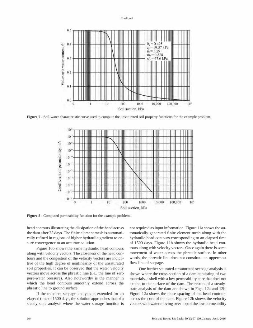
head contours illustrating the dissipation of the head acrossthe dam after 25 days. The finite element mesh is automati-cally refined in regions of higher hydraulic gradient to en-sure convergence to an accurate solution.
Figure 10b shows the same hydraulic head contoursalong with velocity vectors. The closeness of the head con-tours and the congestion of the velocity vectors are indica-tive of the high degree of nonlinearity of the unsaturatedsoil properties. It can be observed that the water velocityvectors move across the phreatic line (i.e., the line of zeropore-water pressure). Also noteworthy is the manner inwhich the head contours smoothly extend across thephreatic line to ground surface.
If the transient seepage analysis is extended for anelapsed time of 1500 days, the solution approaches that of asteady-state analysis where the water storage function is
not required as input information. Figure 11a shows the au-tomatically generated finite element mesh along with thehydraulic head contours corresponding to an elapsed timeof 1500 days. Figure 11b shows the hydraulic head con-tours along with velocity vectors. Once again there is somemovement of water across the phreatic surface. In otherwords, the phreatic line does not constitute an uppermostflow line of seepage.
One further saturated-unsaturated seepage analysis isshown where the cross-section of a dam consisting of twomaterials, a shell with a low permeability core that does notextend to the surface of the dam. The results of a steady-state analysis of the dam are shown in Figs. 12a and 12b.Figure 12a shows the close spacing of the head contoursacross the core of the dam. Figure 12b shows the velocityvectors with water moving over-top of the low permeability
104 Soils and Rocks, São Paulo, 39(1): 97-109, January-April, 2016.
Fredlund
Figure 7 - Soil-water characteristic curve used to compute the unsaturated soil property functions for the example problem.
Figure 8 - Computed permeability function for the example problem.

core through a syphon effect. The results indicate that it iseasier for the water to flow upward through the unsaturatedsoil rather than to flow through the lower permeability corematerial. The siphon phenomenon was one of the early un-saturated soils that intrigued geotechnical engineers but isnow readily explainable through use of saturated-unsa-turated seepage analysis (Terzghi, 1943).
8. Use of Automatic Adaptive MeshRefinement for Saturated Seepage Examples
Automatic adaptive mesh generation and refinementcan also be used to advantage when modeling saturated-unsaturated seepage problems. Two example problems in-
volving seepage through a saturated soil were analyzed byChapuis (2012). These examples are re-analyzed taking ad-vantage of automatic mesh generation and refinement. Theexample problems were solved using automatic mesh re-finement, AMR, programmed in the SVFlux - FlexPDE fi-nite element code.
8.1. Cut-off example
The geometry of the model dam analyzed is shown inFig. 13. The dam has a partial cut-off wall and the soil has asaturated coefficient of permeability of 8.13 x 10⁻³ m/day.
Chapuis (2012) obtained converged solutions using auniform mesh with an element size of 0.5 m. Figure 13
Soils and Rocks, São Paulo, 39(1): 97-109, January-April, 2016. 105
Numerical Modeling of Unsaturated Soils Problems
Figure 9 - Computed water storage function for the example problem.
Figure 10 - a) Finite element mesh and hydraulic heads after the reservoir level was raised for 25 days. b) Velocity vectors and hydraulicheads after the reservoir level was raised for 25 days.

shows that the converged solution obtained when using theautomatic adaptive mesh refinement has larger elements inmost parts of the analyzed domain. The exception is aroundthe cut-off wall where the finite element sizes are signifi-cantly smaller than the overall average element size. For the
mesh shown in Fig. 13, the calculated flow rate was6.82 x 10-7 m3/s using the automatic mesh refinement codeof SVFlux - FlexPDE. A comparison of seepage rate resultsobtained when using manually-controlled mesh and the au-tomatic-controlled adaptive mesh are shown in Fig. 14. The
106 Soils and Rocks, São Paulo, 39(1): 97-109, January-April, 2016.
Fredlund
Figure 11 - a) Finite element mesh and hydraulic heads after the reservoir level was raised for 1500 days. b) Velocity vectors and hydrau-lic heads after the reservoir level was raised for 1500 days.
Figure 12 - a) Finite element mesh and hydraulic heads under steady state conditions. b) Velocity vectors and hydraulic heads understeady state conditions.

automatic adaptive mesh refinement technique requiredconsiderably less computer time to obtain an accurate solu-tion.
8.2. Confined aquifer example
The geometry of the second example problem is pre-sented in Fig. 15. The pumping well is in a confined aquiferwith a saturated coefficient of permeability of 4.0 x 10⁻⁴ m/s.
Figure 15 shows the model geometry with the finiteelement mesh generated using the adaptive generator.
There are some triangular elements that have angles largerthan 90 degrees and this is not the preferred shape for calcu-lation purposes. The problem is axisymmetric with a radiusof 600 m. The converged solution when using a uniformmesh occurred with an element size of 0.1 m (Chapuis,2012). The same problem was solved using automatic meshrefinement in the SVFlux - FlexPDE code. The convergedsolution obtained using the automatic adaptive mesh haslarger elements in most parts of the analyzed domain withthe exception of the region around the pumping well wherethe element size is significantly smaller. For the mesh pre-sented in Fig. 15 the computed flow-rate was 369.2 m3/day.
Figure 16 shows a comparison of the flow-rate ob-tained when the mesh was manually-controlled and whenthe mesh was automatically generated using adaptive meshrefinement. Figure 17 shows a comparison of the total headcalculated at the well.
The results from the reported study indicate that theuse of a finer mesh does not necessarily provide a more ac-curate solution. The primary concern is that the calculatedresult can be in error if the finite element mesh is not suffi-ciently refined. The results obtained when using automaticadaptive mesh refinement procedure can have larger ele-ments over most parts of the domain while the accuracy ofthe solution remains preserved.
Soils and Rocks, São Paulo, 39(1): 97-109, January-April, 2016. 107
Numerical Modeling of Unsaturated Soils Problems
Figure 13 - Partial cut-off wall model geometry with mesh generated using the automatic adaptive mesh generator.
Figure 14 - Converged leakage flow-rate for the cut-off example.
Figure 15 - Pumping well in a confined aquifer.
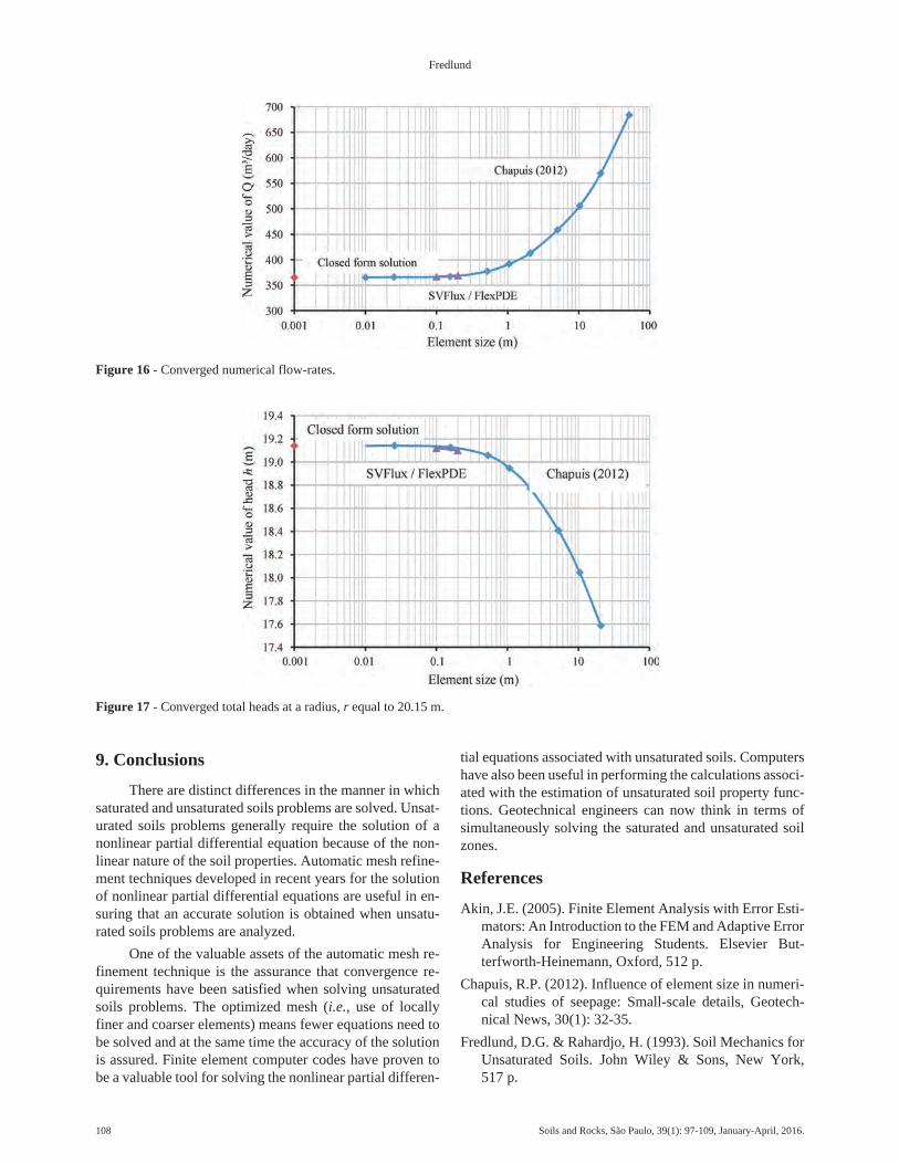
9. Conclusions
There are distinct differences in the manner in whichsaturated and unsaturated soils problems are solved. Unsat-urated soils problems generally require the solution of anonlinear partial differential equation because of the non-linear nature of the soil properties. Automatic mesh refine-ment techniques developed in recent years for the solutionof nonlinear partial differential equations are useful in en-suring that an accurate solution is obtained when unsatu-rated soils problems are analyzed.
One of the valuable assets of the automatic mesh re-finement technique is the assurance that convergence re-quirements have been satisfied when solving unsaturatedsoils problems. The optimized mesh (i.e., use of locallyfiner and coarser elements) means fewer equations need tobe solved and at the same time the accuracy of the solutionis assured. Finite element computer codes have proven tobe a valuable tool for solving the nonlinear partial differen-
tial equations associated with unsaturated soils. Computershave also been useful in performing the calculations associ-ated with the estimation of unsaturated soil property func-tions. Geotechnical engineers can now think in terms ofsimultaneously solving the saturated and unsaturated soilzones.
References
Akin, J.E. (2005). Finite Element Analysis with Error Esti-mators: An Introduction to the FEM and Adaptive ErrorAnalysis for Engineering Students. Elsevier But-terfworth-Heinemann, Oxford, 512 p.
Chapuis, R.P. (2012). Influence of element size in numeri-cal studies of seepage: Small-scale details, Geotech-nical News, 30(1): 32-35.
Fredlund, D.G. & Rahardjo, H. (1993). Soil Mechanics forUnsaturated Soils. John Wiley & Sons, New York,517 p.
108 Soils and Rocks, São Paulo, 39(1): 97-109, January-April, 2016.
Fredlund
Figure 16 - Converged numerical flow-rates.
Figure 17 - Converged total heads at a radius, r equal to 20.15 m.

Fredlund, D.G.; Rahardjo, H. & Fredlund, M.D. (2012).Unsaturated Soil Mechanics in Engineering Practice.John Wiley & Sons, New York, 926 p.
Fredlund, D.G. & Stianson, J. (2011). Utilization of wea-ther station data for the assessment of ground surfacemoisture fluxes. Proc. Fifth Asia-Pacific Conference onUnsaturated Soils, Payatta, Thailand, pp. 1-18.
Fredlund, M.D. (2012). SVFlux User’s Manual. SoilVisionSystems Ltd. Saskatoon, Canada, 112 p.
Fredlund, M.D.; Zhang, J.M.; Tran, D. & Fredlund, D.G.(2011). Coupling heat and moisture flow for the compu-tation of actual evaporation.Proc. Canadian Geotech-nical Conference and Fifth Pan-American Conference,Toronto, Paper 1058.
Oberkampf, W.L.; Blottner, F.G. & Aeschliman, D.P.(1995). Methodology for computational fluid dynamicscode verification/validation. Proc. AIAA Fluid Dynam-ics Conference, San Diego, Paper 95-2226.
Petrovic, I. & Fredlund, M.D. (2012). Benefits of adaptivemesh refinement. Geotechnical News, 30(4): 37-40.
Reddy, J.N. (2006). An Introduction to the Finite ElementMethod. McGraw-Hill, Boston, 784 p.
Roache P.J. (2009). Fundamentals of Verification and Vali-dation. Hermosa Publishers, Socorro, 648 p.
Terzaghi, K. (1943). Theoretical Soil Mechanics. Wiley,New York, 510 p.
Tran, Dat Tien Quoc (2013). Re-Visitation of Actual Evap-oration Theories. Ph.D. Thesis, University of Alberta,Edmonton, 420 p.
Wilson, G.W. (1990). Soil Evaporative Fluxes for Geo-technical Engineering Problems. PhD Thesis, Depart-ment of Civil and Geological Engineering, Universityof Saskatchewan, 464 p.
Wilson, G.W.; Fredlund, D.G. & Barbour, S.L. (1994).Coupled soil-atmospheric modeling for soil evapora-tion, Canadian Geotechnical Journal, 31(2):151-161.
Zienkiewicz, O.C.; Taylor, R.L. & Zhu, J.Z. (2005) The Fi-nite Element Method: Its Basis and Fundamentals.Elsevier Butterfworth-Heinemann, Oxford, 752 p.
Soils and Rocks, São Paulo, 39(1): 97-109, January-April, 2016. 109
Numerical Modeling of Unsaturated Soils Problems

SOILS and ROCKSAn International Journal of Geotechnical and Geoenvironmental Engineering
Publication ofABMS - Brazilian Association for Soil Mechanics and Geotechnical Engineering
SPG - Portuguese Geotechnical SocietyVolume 39, N. 1, January-April 2015
Author index
Cordão Neto, M.P. 29Fredlund, D.G. 3, 81, 97G.F.N. Gitirana Jr., 81Gomes, I. 19Guimarães, L. 19Krisnanto, S. 51Leong, E.C. 51Lima, A. 19
Lins, C. 19Mascarenha, M.M.A. 29Oh, W.T. 71Rahardjo, H. 51Sheng, D. 41Silva, M.T.M.G. 29Silva, N. 19Vanapalli, S.K. 71


Instructions for Submission of ManuscriptsCategory of the Papers
Soils and Rocks is the international scientific journaledited by the Brazilian Association for Soil Mechanicsand Geotechnical Engineering (ABMS) and the Portu-guese Geotechnical Society (SPG). The aim of the jour-nal is to publish (in English) original research andtechnical works on all geotechnical branches.
According to its content the accepted paper is classi-fied in one of the following categories: Article paper,Technical Note, Case Study or Discussion. An article pa-per is an extensive and conclusive dissertation about ageotechnical topic. A paper is considered as a technicalnote if it gives a short description of ongoing studies,comprising partial results and/or particular aspects of theinvestigation. A case study is a report of unusual prob-lems found during the design, construction or the perfor-mance of geotechnical projects. A case study is alsoconsidered as the report of an unusual solution given to anordinary problem. The discussions about published pa-pers, case studies and technical notes are made in the Dis-cussions Section.
When submitting a manuscript for review, the authorsshould indicate the category of the manuscript, and is alsounderstood that they:
a) assume full responsibility for the contents and ac-curacy of the information in the paper;
b) assure that the paper has not been previously pub-lished, and is not being submitted to any other periodicalfor publication.Manuscript Instructions
Manuscripts must be written in English. The text is tobe typed in a word processor (preferably MS Word), sin-gle column, using ISO A4 page size, left, right, top, andbottom margins of 25 mm, Times New Roman 12 font,and line spacing of 1.5. All lines and pages should benumbered. The text should be written in the third person.
The first page of the manuscript must include the titleof the paper followed by the names of the authors with theabbreviation of the most relevant academic title. The af-filiation, address and e-mail must appear below each au-thor´s name. An abstract of 200 words follows after theauthor´s names. A list with up to six keywords at the endof the abstract is required.
Although variations on the sequence and title of eachsection are possible, it is suggested that the text containsthe following sections: Introduction, Material andMethods, Results, Discussions, Conclusions, Acknowl-edgements, References and List of Symbols. A brief de-scription of each section is given next.
Introduction: This section should indicate the stateof the art of the problem under evaluation, a descriptionof the problem and the methods undertaken. The objec-tive of the work should be clearly presented at the end ofthe section.
Materials and Methods: This section should includeall information needed to the reproduction of the pre-sented work by other researchers.
Results: In this section the data of the investigationshould be presented in a clear and concise way. Figuresand tables should not repeat the same information.
Discussion: The analyses of the results should be de-scribed in this section.
Conclusions: The content of this section should be based on the dataand on the discussions presented.
Acknowledgenments: If necessary, concise acknowledgementsshould be presented in this section.
References: References to other published sources must be made inthe text by the last name(s) of the author(s), followed by the year of publi-cation, similarly to one of the two possibilities below:
…while Silva and Pereira (1987) observed that resistance dependedon soil density… or It was observed that resistance depended on soil den-sity (Silva and Pereira, 1987).
In the case of three or more authors, the reduced format must be used,e.g.: Silva et al. (1982) or (Silva et al., 1982). Two or more citations be-longing to the same author(s) and published in the same year are to be dis-tinguished with small letters, e.g.: (Silva, 1975a, b, c.). Standards must becited in the text by the initials of the entity and the year of publication, e.g.:ABNT (1996), ASTM (2003).
Full references shall be listed alphabetically at the end of the text bythe first author´s last name. Several references belonging to the same au-thor shall be cited chronologically. Some examples are listed next:Papers: Bishop, A.W. & Blight, G.E. (1963). Some aspects of effective
stress in saturated and unsaturated soils. Geotechnique, 13(2):177-197.
Books: Lambe, T.W & Whitman, R.V. (1979). Soil Mechanics, SI Ver-sion. John Wiley & Sons, New York, 553 p.
Book with editors: Sharma, H.D.; Dukes, M.T. & Olsen, D.M. (1990).Field measurements of dynamic moduli and Poisson’s ratios of refuseand underlying soils at a landfill site. Landva, A. & Knowles, G.D.(eds), Geotechnics of Waste Fills - Theory and Practice, American So-ciety for Testing and Materials - STP 1070, Philadelphia, pp. 57-70.
Proceedings (printed matter or CD-ROM): Jamiolkowski, M.; Ladd,C.C.; Germaine, J.T. & Lancellotta, R. (1985). New developments infield and laboratory testing of soils. Proc. 11th Int. Conf. on SoilMech. and Found. Engn., ISSMFE, San Francisco, v. 1, pp. 57-153.(specify if CD ROM).
Thesis and dissertations: Lee, K.L. (1965). Triaxial CompressiveStrength of Saturated Sands Under Seismic Loading Conditions. PhDDissertation, Department of Civil Engineering, University of Califor-nia, Berkeley, 521 p.
Standards: ASTM (2003). Standard Test Method for Particle Size Analy-sis of Soils - D 422-63. ASTM International, West Conshohocken,Pennsylvania, USA, 8 p.
Internet references: Soi ls and Rocks avai lable athttp://www.abms.com.br and downloaded on August 6th 2003.
On line first publications must also bring the digital object identifier(DOI) at the end.Figures shall be either computer generated or drawn with India ink on
tracing paper. Computer generated figures must be accompanied by thecorresponding digital file (.tif, .jpg, .pcx, etc.). All figures (graphs, linedrawings, photographs, etc.) shall be numbered consecutively and have acaption consisting of the figure number and a brief title or description ofthe figure. This number should be used when referring to the figure in text.Photographs should be black and white, sharp, high contrasted andprinted on glossy paper.
Tables shall be numbered consecutively in Arabic and have a captionconsisting of the table number and a brief title. This number should beused when referring to the table in the text. Units should be indicated inthe first line of the table, below the title of each column. Acronyms shouldbe avoided. When applicable, the units should come right below the cor-responding column heading. Additional comments can be placed as foot-notes.
Equations shall appear isolated in a single line of the text. Numbersidentifying equations must be flushed with the right margin. InternationalSystem (SI) units must be used. The definitions of the symbols used in the

equations must appear in the List of Symbols. It is recom-mended that the symbols used are in accordance withLexicon in 8 Languages, ISSMFE (1981) and the ISRMList of Symbols.
The text of the submitted manuscript (including fig-ures, tables and references) intended to be published as anarticle paper or a case history should not contain morethan 30 pages, formatted according to the instructionsmentioned above. Technical notes and discussionsshould have no more than 15 and 8 pages, respectively.Longer manuscripts may be exceptionally accepted if theauthors provide proper explanation for the need of the re-quired extra space in a cover letter.Discussion
Discussions must be written in English. The first pageof a discussion should contain:
The title of the paper under discussion;Name of the author(s) of the discussion, followed by
their position, affiliation, address and e-mail. The au-thor(s) of the discussion should refer to himself (her-self/themselves) as the reader(s) and to the author(s) ofthe paper as the author(s).
Figures, tables and equations should be numbered following the samesequence of the original paper. All instructions previously mentioned forthe preparation of article papers, case studies and technical notes also ap-ply to the preparation of discussions.Editorial Review
Each paper will be evaluated by reviewers selected by the editors ac-cording to the subject of the paper. The authors will be informed about theresults of the review process. If the paper is accepted, the authors will berequired to submit a version of the revised manuscript with the suggestedmodifications. If the manuscript is rejected for publication, the authorswill be informed about the reasons for rejection. In any situation compris-ing modification of the original text, classification of the manuscript in acategory different from that proposed by the authors, or rejection, the au-thors can reply presenting their reasons for disagreeing with the reviewercomments.Submission
The author(s) must upload a digital file of the manuscript to the Soilsand Rocks website.Follow Up
The online management system will provide a password to the corre-sponding author, which will enable him/her to follow the reviewing pro-cess of the submitted manuscript at the Soils and Rocks website.

Volume , NJanuary-April 2016
39 . 1
Soils and RocksAn International Journal of Geotechnical
and Geoenvironmental Engineering
SOILS and ROCKS An nternational Journal of Geotechnical and Geoenvironmental EngineeringI
Volume , N. 1, January-April 201639
Table of Contents
Soils and R
ocks Volume 39, N
. 1 2016
ISSN 980-97431
BMS
ARTICLES
State Variables in Saturated-Unsaturated Soil Mechanics
Numerical and Experimental Analysis of Horizontal Stress Changes and Soil Collapse DuringChemical Dissolution in a Modified Oedometer Cell
Alternative Method for Analysing Hydromechanical Behaviour of Unsaturated Soils
Recent Developments and Limitations of the SFG Model
Effectiveness of Capillary Barrier and Vegetative Slope Covers in Maintaining Soil Suction
Influence of Poisson’s Ratio on the Stress vs. Settlement Behavior of Shallow Foundations inUnsaturated Fine-Grained Soils
Statistical Assessment of Hydraulic Properties of Unsaturated Soils
Numerical Modeling of Unsaturated Soils Problems
D.G. Fredlund 3
C. Lins, N. Silva, L. Guimarães, A. Lima, I. Gomes 19
M.M.A. Mascarenha, M.P. Cordão Neto, M.T.M.G. Silva 29
D. Sheng 41
H. Rahardjo, S. Krisnanto, E.C. Leong 51
W.T. Oh, S.K. Vanapalli 71
G.F.N. Gitirana Jr., D.G. Fredlund 81
M.D. Fredlund 97
Special Issue: Unsaturated SoilsGuest editors:
G.F.N. Gitirana Jr. & D.G. Fredlund
0
5
25
75
95
100
0
5
25
75
95
100
0
5
25
75
95
100
0
5
25
75
95
100