ISPRS Journal of Photogrammetry and Remote Sensing 129 (2017) 12–20

Contents lists available at ScienceDirect

ISPRS Journal of Photogrammetry and Remote Sensing

journal homepage: www.elsevier .com/ locate/ isprs jprs

Automatic detection of Martian dark slope streaks by machine learningusing HiRISE images

http://dx.doi.org/10.1016/j.isprsjprs.2017.04.0140924-2716/� 2017 International Society for Photogrammetry and Remote Sensing, Inc. (ISPRS). Published by Elsevier B.V. All rights reserved.

⇑ Corresponding author.E-mail address: dikc@radi.ac.cn (K. Di).

Yexin Wang, Kaichang Di ⇑, Xin Xin, Wenhui WanState Key Laboratory of Remote Sensing Science, Institute of Remote Sensing and Digital Earth, Chinese Academy of Sciences, No. 20A, Datun Road, Chaoyang District, Beijing100101, China

a r t i c l e i n f o

Article history:Received 13 January 2016Received in revised form 15 March 2017Accepted 24 April 2017

Keywords:Dark slope streakMartian surfaceMachine learningHiRISE imageRegion detection

a b s t r a c t

Dark slope streaks (DSSs) on the Martian surface are one of the active geologic features that can beobserved on Mars nowadays. The detection of DSS is a prerequisite for studying its appearance, morphol-ogy, and distribution to reveal its underlying geological mechanisms. In addition, increasingly massiveamounts of Mars high resolution data are now available. Hence, an automatic detection method for locat-ing DSSs is highly desirable. In this research, we present an automatic DSS detection method by combin-ing interest region extraction and machine learning techniques. The interest region extraction combinesgradient and regional grayscale information. Moreover, a novel recognition strategy is proposed thattakes the normalized minimum bounding rectangles (MBRs) of the extracted regions to calculate theLocal Binary Pattern (LBP) feature and train a DSS classifier using the Adaboost machine learning algo-rithm. Comparative experiments using five different feature descriptors and three different machinelearning algorithms show the superiority of the proposed method. Experimental results utilizing 888extracted region samples from 28 HiRISE images show that the overall detection accuracy of our pro-posed method is 92.4%, with a true positive rate of 79.1% and false positive rate of 3.7%, which in partic-ular indicates great performance of the method at eliminating non-DSS regions.� 2017 International Society for Photogrammetry and Remote Sensing, Inc. (ISPRS). Published by Elsevier

B.V. All rights reserved.

1. Introduction

Dark slope streaks (DSSs) are seen on the surface of Mars asdark, narrow, fan shaped features (e.g., Fig. 1) that appear on slopescovered by dust at low latitudes (Schörghofer, 2014). Observationsfrom multiple coverage images show that fresh DSSs are darkerthan their surrounding area, then gradually fade away over time,finally merging with the background and disappearing (Carr,2007; Gremminger, 2005–2006). The interest in investigating DSSarises because it is one of the active geologic features that can cur-rently be observed on Mars. Study of its morphologies, distribu-tions and changes, (Sullivan et al., 2001; Schorghofer and King,2011) are important for revealing and understanding its formationmechanisms (Burleigh et al., 2012; King 2005–2006; Aharonsonet al., 2003), inner geological structure (Gerstell et al., 2004), rela-tions with atmospheric action (Cantor, 2007; Chuang et al., 2010;Baratoux et al., 2006), surface composition (Ojha et al., 2015),

and other fields (Schorghofer et al., 2002). Before these studiescan be carried out, detection of DSSs is the first basic step.

According to Baratoux’s statistics (Baratoux et al., 2006), thewidths of DSSs mostly range from 25 to 125 m, and many streakscan only be clearly observable and confirmed on high resolutionimages. In the past, this work was mainly done manually(Schorghofer et al., 2002; Bergonio et al., 2013; Chuang et al.,2007). Currently, high resolution data from several missions arestill being released each year. Nevertheless, the coverage of Marsat a resolution finer than 2 m/pixel is still low. In the near future,there will be more missions carrying high resolution sensors. Withthe increasingly massive amounts of Mars high resolution dataavailable now and in the future, an automatic detection methodis highly desirable.

Before the development of automatic approaches, manualextraction method was used: Schorghofer et al. (2007) studiedslope steak activity in five areas by manually comparing Vikingobservations in 1977–1980 and Mars Orbiter Camera (MOC) obser-vations 1998–2005; Aharonson et al. (2003) performed a globalanalysis of the slope streaks by manually examining 29,326 MOCnarrow angle images and found slope streaks in 1386 images;Baratoux et al. (2006) manually identified and measured the

Fig. 1. Examples of DSSs on Mars. HiRISE observation IDs are given below each subfigure. All the images are stretched for contrast enhancement. The scale bar in eachsubfigure is 100 m, and north is up.

Y. Wang et al. / ISPRS Journal of Photogrammetry and Remote Sensing 129 (2017) 12–20 13

lengths, widths, and directions of DSSs in two regions and analyzedthese properties with respect to factors such as terrain, wind direc-tion, and surface roughness.

As manual work is time consuming, some automatic DSSextraction methods have been developed recently. Di et al.(2014a) used a context window that calculates the grayscale gradi-ents for each pixel in the image, then set a threshold to choose thepixels that have high contrast against the background to form theDSS regions. However, the work did not include a recognitionstage, so the extracted regions need the further confirmation ofan expert. Wagstaff et al. (2012) computed the entropy in a localwindow for every pixel and picked the pixels with entropy higherthan a certain threshold to form a region. They then used its shapeproperties and simple grayscale information to train a classifier.For DSSs that are located in more complicated backgrounds, theseregion descriptions are not sufficient to describe the target. Giventhe few previous works on DSS detection, machine learning is apromising approach that would save manual recognition time.

For other geology features, especially for craters, numerousmachine learning detection methods have been proposed (Burlet al., 2001; Vinogradova et al., 2002; Martins et al., 2009; Dinget al., 2013; Cohen and Ding, 2014; Di et al., 2014b). Given cratercharacteristics, a window-based machine learning method isalways employed. The typical way to implement a window-basedmachine learning approach is to use square windows that eachincludes a crater as positive samples, and windows without cratersas negative samples. Then a feature description method is used toextract the characteristics of both positive and negative samples.With the extracted feature descriptions and the labels of the sam-ples, a machine learning model is applied to train a classifier. Whentesting a new image, multiple scale sliding square windows areused to traverse the entire image, and the classifier is used to judgewhether the current square window contains a crater. The finalresults are obtained by eliminating the reduplicative squares. Ifthe contour of the crater is needed, edge extraction and ellipse fit-

ting should be done in the identified square (Kim and Muller,2005). Because a DSS is slender and often appears very close toadjacent ones, the window-based method is not appropriate in thiscase. Using this window-based method, in some cases, a DSS mayonly cover a small part of the entire window, meanwhile the win-dow may include portions of adjacent DSSs and other surface fea-tures (see Fig. 1). In this way, the features for describing a windowcontaining a DSS as positive samples are indistinguishable enoughsuch that an effective classification is not achievable (Cheng et al.,2014). Another mode of pattern recognition is to use object-basedmethods (Chen et al., 2014; Blaschke, 2010; Mallinis et al., 2008),i.e., first forming regions obtained by a certain segmentation algo-rithm (such as those described in Di et al. (2014a) and Wagstaffet al. (2012) and other methods: clustering (Maulik and Saha,2010), region growing (Yu and Clausi, 2008), etc.), and then train-ing the classifier using the features extracted from the regions. Thesegmentation step must be applied to the new images for identifi-cation before applying the classifier. However, object-based recog-nition methods only focus on grayscale or shape features withinthe contour, ignoring the adjacent grayscale information, whichis the prominent characteristic of a DSS. A DSS lacks texture infor-mation on its surface, hence the grayscale difference between theinside and outside of the DSS is its distinguishable characteristic.If this information can be taken into account, it may improve therecognition accuracy.

In this study, we present an automatic DSS detection approachthat combines region extraction and machine learning techniques.The data used in this study is briefly introduced in Section 2. InSection 3, we first present the interest region extraction processthat combines gradient and regional grayscale information. A novelrecognition strategy that considers the texture inside the extractedregions as well as the imaging characteristics of its surroundingarea is then proposed. Section 4 presents the experiment resultsbased on our proposed method. Finally, the conclusion is given inSection 5.

14 Y. Wang et al. / ISPRS Journal of Photogrammetry and Remote Sensing 129 (2017) 12–20

2. Data

As mentioned in the previous section, because of the smallwidth of DSSs, they are only clearly observable on high resolutionimages. In contrast to two high resolution data sets obtained by theMOC narrow angle camera (resolution of 1.4 m/pixel, stop releas-ing new data since November 2006) and the High ResolutionStereo Camera (HRSC) (resolution up to 2 m/pixel), HiRISE imageshave a resolution up to 0.25 m/pixel, and large amounts of newdata are being released every few days. Therefore, the work donein this paper is based on the HiRISE images. More specifically,the Reduced Data Record products of the HiRISE data, which havebeen radiometrically corrected, geometrically rectified, and mapprojected (downloadable from the HiRISE website http://www.uahirise.org/) are used in this study. We use 34 HiRISE images totest our method. The distribution of the images is shown inFig. 2. The yellow dots represent the center locations of the HiRISEimages. All the images are selected from dust cover area at low lat-itudes, which are the areas in which DSSs most likely lie.

3. Method

The automatic DSS detection method consists of interest regionextraction, classifier training, and new data recognition. First, theinterest region extraction process extracts region candidates thatmay include DSSs. Local Binary Pattern (LBP) features are then cal-culated from the normalized minimum bounding rectangles(MBRs) of the interest regions. In this way, features inside and out-side the regions can both function. After that, a DSS classifier istrained based on these extracted features. When new data needsto be identified by the classifier, interest region extraction andLBP calculation from MBRs should be done beforehand.

3.1. Interest region extraction

Generally, DSSs appear in groups, i.e., there are fresh, slightlyfading, and mostly faded DSSs clustered in the same area. Our

Fig. 2. Distribution of the HiRISE

aim is to extract the contours and provide the location informationof the fresh and slightly fading ones. In this subsection, we presentan interest region extraction method to automatically extractregions that likely contain DSSs for both training the classifierand recognizing new data (described in the next section). The flow-chart of the proposed region extraction method is shown in Fig. 3.

Note that the HiRISE image is large, therefore preprocessing isaccomplished on divided sub-images. According to the size of theHiRISE images, we divide each image into sub-images with 50%overlapping area in each direction to ensure a DSS is not cut in half.The sub-images are preprocessed by successively using imageadaptive enhancement, median filtering and mean filtering inorder to increase contrast and remove noises. Then the imagesafter preprocessing are recursively convolved by Deriche operatorto extract the edges. The Deriche operator is based on Canny prin-ciples, and filters the images recursively in both x and y directions.The edge direction and amplitude are calculated based on the con-volution results, then the amplitude is non-maximum suppressedin the computed direction and a hysteresis threshold is used toobtain the extracted edges. Further technical details can be foundin Deriche (1987).

The Deriche operator provides excellent edge detection resultsby considering the local gradient information. When applying iton HiRISE images, some unwanted edges such as ridge lines andgullies cannot be removed by a simple principle such as lengththreshold. At the HiRISE resolution, DSSs are imaged as darkregions of length ranging from hundreds to thousands pixels. Giventhis feature, not just local but regional information in a large areashould be considered. In this case, a sliding square window ofwidth w is considered over the entire image, comparing the grayvalue of the center pixel I(x, y) to the average gray value of the cur-rent window:

Hðx; yÞ ¼ Iðx; yÞ � 1w2

X

ðm;nÞ2WIðm;nÞ ð1Þ

where I(m, n) represents the gray value of each pixel in window W.Threshold D is set to preserve the pixels that have high contrast

images used in this study.

HiRISE image

Window-based grayscale information calculation

Is the edge-region intersectiongreater than the threshold?

Y

N

Small region elimination using morphological processing and area

threshold

Preprocessing

Deriche operator

Short edges elimination using length threshold

Edge elimination

Edge linking to form region candidate

Fig. 3. Flowchart of the interest region extraction method.

Y. Wang et al. / ISPRS Journal of Photogrammetry and Remote Sensing 129 (2017) 12–20 15

with respect to the background to form dark regions. In practice, weadopt a 50 � 50 pixels window and D is set to 20 (for gray valuesranging from 0 to 255 in our 8-bit images). In order to reduce cal-culation time, only pixels with gray values less than 120 are usedin this window-based detection. Small noise regions extracted bythe window-based method are eliminated by morphological open-ing and closing operations and small area thresholding. The remain-ing regions are expanded with a disk-shaped structure element ofradius 3. If 70% of the length of an edge extracted by the Derichemethod is in one of the regions, we keep the edge. Otherwise, theedge is eliminated. In this way, most undesired edges are removed.Finally, the remaining edge pieces are linked by adjacent and simi-lar direction properties in order to form the interest regions for thesubsequent processing.

Fig. 4 shows some of the extraction results. Fig. 4(a) shows sev-eral extracted DSSs. Fig. 4(b) shows a case where in addition to theDSSs, other areas are also extracted at the bottom of the image. Thetwo images also show that some fading DSSs are merged with thebackground or other dark areas, hence they are not extracted.Because of the lighting, some terrain fluctuation regions such asridges and ravines on the images may also be extracted, as shownin Fig. 4(c). As we can see from Fig. 4, the extracted interest regions

Fig. 4. Some examples of interest region extraction results. T

contain DSSs and other kinds of land features. Hence, patternrecognition should be performed to pick out the DSSs. This processis introduced in the next section.

3.2. LBP feature calculation in normalized MBRs

By extracting various region properties or calculating the grays-cale statistics such as mean and variance, the region candidatesderived in the previous subsection can be used directly for tradi-tional object-based recognition method. However, as mentionedabove, these properties are not sufficient and appropriate for adetailed description of DSS. Because of the various shapes of theinterest regions, more complex description operators such as LBP(Ojala et al., 1996), Histogram of Oriented Gradient (HOG) Dalaland Triggs, 2005, and Haar-like (Lienhart and Maydt, 2002) fea-tures, which provide more precise description, are impractical tocalculate. To solve this problem as well as utilize the grayscale dif-ference both inside the DSS region and around it, we propose tocalculate these complex features in the minimum bounding rect-angle (MBR) of the extracted interest region. As the shapes andsizes of the interest regions vary and the directions of the rectan-gles are stochastic, we further propose to normalize the MBRs

he scale bar in each subfigure is 100 m, and north is up.

16 Y. Wang et al. / ISPRS Journal of Photogrammetry and Remote Sensing 129 (2017) 12–20

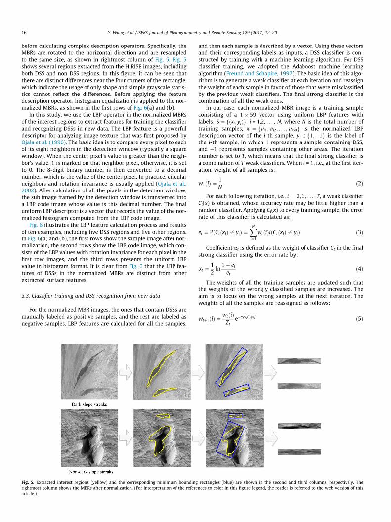
before calculating complex description operators. Specifically, theMBRs are rotated to the horizontal direction and are resampledto the same size, as shown in rightmost column of Fig. 5. Fig. 5shows several regions extracted from the HiRISE images, includingboth DSS and non-DSS regions. In this figure, it can be seen thatthere are distinct differences near the four corners of the rectangle,which indicate the usage of only shape and simple grayscale statis-tics cannot reflect the differences. Before applying the featuredescription operator, histogram equalization is applied to the nor-malized MBRs, as shown in the first rows of Fig. 6(a) and (b).

In this study, we use the LBP operator in the normalized MBRsof the interest regions to extract features for training the classifierand recognizing DSSs in new data. The LBP feature is a powerfuldescriptor for analyzing image texture that was first proposed byOjala et al. (1996). The basic idea is to compare every pixel to eachof its eight neighbors in the detection window (typically a squarewindow). When the center pixel’s value is greater than the neigh-bor’s value, 1 is marked on that neighbor pixel, otherwise, it is setto 0. The 8-digit binary number is then converted to a decimalnumber, which is the value of the center pixel. In practice, circularneighbors and rotation invariance is usually applied (Ojala et al.,2002). After calculation of all the pixels in the detection window,the sub image framed by the detection window is transferred intoa LBP code image whose value is this decimal number. The finaluniform LBP descriptor is a vector that records the value of the nor-malized histogram computed from the LBP code image.

Fig. 6 illustrates the LBP feature calculation process and resultsof ten examples, including five DSS regions and five other regions.In Fig. 6(a) and (b), the first rows show the sample image after nor-malization, the second rows show the LBP code image, which con-sists of the LBP values with rotation invariance for each pixel in thefirst row images, and the third rows presents the uniform LBPvalue in histogram format. It is clear from Fig. 6 that the LBP fea-tures of DSSs in the normalized MBRs are distinct from otherextracted surface features.

3.3. Classifier training and DSS recognition from new data

For the normalized MBR images, the ones that contain DSSs aremanually labeled as positive samples, and the rest are labeled asnegative samples. LBP features are calculated for all the samples,

Fig. 5. Extracted interest regions (yellow) and the corresponding minimum boundingrightmost column shows the MBRs after normalization. (For interpretation of the referearticle.)

and then each sample is described by a vector. Using these vectorsand their corresponding labels as inputs, a DSS classifier is con-structed by training with a machine learning algorithm. For DSSclassifier training, we adopted the Adaboost machine learningalgorithm (Freund and Schapire, 1997). The basic idea of this algo-rithm is to generate a weak classifier at each iteration and reassignthe weight of each sample in favor of those that were misclassifiedby the previous weak classifiers. The final strong classifier is thecombination of all the weak ones.

In our case, each normalized MBR image is a training sampleconsisting of a 1 � 59 vector using uniform LBP features withlabels: S ¼ fðxi; yiÞg, i = 1,2, . . . , N, where N is the total number oftraining samples, xi ¼ fv i1;v i2; . . . ;v i59g is the normalized LBPdescription vector of the i-th sample, yi 2 f1;�1g is the label ofthe i-th sample, in which 1 represents a sample containing DSS,and �1 represents samples containing other areas. The iterationnumber is set to T, which means that the final strong classifier isa combination of T weak classifiers. When t = 1, i.e., at the first iter-ation, weight of all samples is:

w1ðiÞ ¼ 1N

ð2Þ

For each following iteration, i.e., t ¼ 2;3; . . . ; T , a weak classifierCt(x) is obtained, whose accuracy rate may be little higher than arandom classifier. Applying Ct(x) to every training sample, the errorrate of this classifier is calculated as:

et ¼ PðCtðxiÞ– yiÞ ¼XN

i¼1

wtðiÞIðCtðxiÞ – yiÞ ð3Þ

Coefficient at is defined as the weight of classifier Ct in the finalstrong classifier using the error rate by:

at ¼ 12ln

1� etet

ð4Þ

The weights of all the training samples are updated such thatthe weights of the wrongly classified samples are increased. Theaim is to focus on the wrong samples at the next iteration. Theweights of all the samples are reassigned as follows:

wtþ1ðiÞ ¼ wtðiÞZt

e�atyiCtðxiÞ ð5Þ

rectangles (blue) are shown in the second and third columns, respectively. Thences to color in this figure legend, the reader is referred to the web version of this

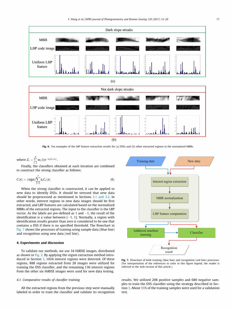
Fig. 6. Ten examples of the LBP feature extraction results for (a) DSSs and (b) other extracted regions in the normalized MBRs.

Fig. 7. Flowchart of both training (blue line) and recognition (red line) processes.(For interpretation of the references to color in this figure legend, the reader isreferred to the web version of this article.)

Y. Wang et al. / ISPRS Journal of Photogrammetry and Remote Sensing 129 (2017) 12–20 17

where Zt ¼PN

i¼1wtðiÞe�atyiCt ðxiÞ.

Finally, the classifiers obtained at each iteration are combinedto construct the strong classifier as follows:

CðxÞ ¼ ðsignÞXT

t¼1

atCtðxÞ ð6Þ

When the strong classifier is constructed, it can be applied tonew data to identify DSSs. It should be stressed that new datashould be preprocessed as mentioned in Sections 3.1 and 3.2. Inother words, interest regions in new data images should be firstextracted, and LBP features are calculated based on the normalizedMBRs of the extracted regions. The input to the classifier is the LBPvector. As the labels are pre-defined as 1 and �1, the result of theidentification is a value between [�1, 1]. Normally, a region withidentification results greater than zero is considered to be one thatcontains a DSS if there is no specified threshold. The flowchart inFig. 7 shows the processes of training using sample data (blue line)and recognition using new data (red line).

4. Experiments and discussion

To validate our methods, we use 34 HiRISE images, distributedas shown in Fig. 2. By applying the region extraction method intro-duced in Section 3, 1024 interest regions were detected. Of theseregions, 888 regions extracted from 28 images were utilized fortraining the DSS classifier, and the remaining 136 interest regionsfrom the other six HiRISE images were used for new data testing.

4.1. Comparative results of classifier training

All the extracted regions from the previous step were manuallylabeled in order to train the classifier and validate its recognition

results. We utilized 208 positive samples and 680 negative sam-ples to train the DSS classifier using the strategy described in Sec-tion 3. About 11% of the training samples were used for a validationtest.

Fig. 9. ROC curves of five different features.

18 Y. Wang et al. / ISPRS Journal of Photogrammetry and Remote Sensing 129 (2017) 12–20

During the training process, we deployed five different descrip-tors for comparison: Haar-like, HOG, region properties (RP), LBP,and LBP combined with RP (LBP + RP) features. Haar-like featureswere calculated on normalized 5 � 25 pixel samples, and the otherdescriptors (not including RP) were computed on 20 � 100 pixelsamples. For the Haar-like descriptor, a total of 558 features wereobtained for each normalized sample. In addition, the numbers ofobtained HOG and LBP descriptors were 3456 and 59, respectively.RP here refers to the characteristics of the extracted regions insteadof those of the MBRs. The RPs used for each sample consisted of 11region shape features including area, the ratio of the region areaand convex-hull area, fitting ellipse properties, compactness, andsix grayscale features such as mean, standard deviation, smooth-ness, and entropy.

Fig. 8 shows the error decreasing curves of the five descriptorsover 100 subsequent iterations. Note that for training, we set thenumber of iterations to 200, yet the fastest decline occurs fromthe 1st to the 50th iteration. After that, the curves decline gently;therefore, we only show the curve to the 100th iteration. InFig. 8, the highest training error is from the method that usedregion properties. The other four are less than 5% after the 50thiteration. This is because the goal of each iteration is to assign aweight on one feature to obtain a weak classifier, and the numberof features in RP is not sufficient to combine into a strong classifier.Haar-like and HOG features have lower errors than the otherdescriptors, which is unsurprising, because the number of featuresare large and Adaboost can build a classification tree by picking themost fitted features in training process to obtain a low error.

The performances of the descriptors are further evaluated usingthe receiver operating characteristic (ROC) curve, which shows therelation between the true positive rate (TPR) and false positive rate(FPR). Fig. 9 shows the ROC curves of five different descriptorsobtained using the validation data. It can be seen that althoughthe HOG and Haar-like features obtain high accuracy in the train-ing phase, they fail to achieve a high TPR in the validation test.The LBP descriptor achieves a higher TPR than the other four whenmaintaining the same FPR. Moreover, Fig. 9 shows the addition ofRP to LBP is not a significant help. Therefore, for describing andidentifying DSS in normalized MBRs, the LBP operator is sufficient.

Using the LBP feature, we also compared the performances ofthree different machine learning algorithms: Adaboost, supportvector machine (SVM) Mountrakis et al., 2011, and neural network(NN) (a ten-hidden-layer feed forward network was used) (Møller,1993). The recognition results are shown in Table 1. The results

Fig. 8. Recognition error of five features in each iteration of the training process.

were calculated based on the validation data. Although samplesfor the validation test account for only 11% of all the samples,the final validation test results are actually based on all the sam-ples. This was implemented by dividing all the samples into ninegroups such that each group had almost the same number of pos-itive and negative samples. Eight groups were used for training aclassifier and the last one was used for validation. This processwas repeated nine times so that each group had the chance to bein the validation test. Table 1 shows that compared to NN and Ada-boost, SVM obtained the worst performance in every respect: high-est FPR, lowest TPR and total accuracy. Although NN has a slightadvantage over Adaboost with respect to TPR, its FPR is much lar-ger than that of Adaboost. To evaluate the different machine learn-ing algorithms in this study, FPR is crucial, as low FPR represents alow error for the elimination of non-DSS regions in all detectedregions, which would significantly reduce labor requirement whenthe data volume is large. Based on this criterion, the Adaboostresults have the lowest FPR and the highest total accuracy, andhence it is the most appropriate algorithm for identifying DSSs.

4.2. DSS recognition from new data

In order to test the classifier, we applied it on new data. Afterinterest region detection and LBP feature calculation from the nor-malized MBRs, the classifier constructed in Section 4.1 takes thenormalized LBP features as inputs and generates the recognitionresult. The preprocessing procedure on the new data before it isclassified is the same as that of the training samples. Note also thatall the training samples were treated like new data when theywere chosen for the validation test. Hence, the detection accuracyof new data is similar to that listed in Table 1.

Fig. 10 shows the recognition results of a sub-image of a HiRISEimage, in which the red rectangles are used to mark the MBRs thatcontain DSSs. Fig. 11 shows additional recognition results. When

Table 1Performance comparison of three different classifiers trained using SVM, NN, andAdaboost.

Evaluation criteria Support vectormachine (SVM)

Neural network(NN)

Adaboost

True positive rate (TPR) % 75.1 80.1 79.1False positive rate (FPR) % 10.9 8.2 3.7Total accuracy % 85.9 89.1 92.4

Fig. 10. Sub image (red rectangle on the left image) of a HiRISE image (ID: ESP_037015_1890) and its detection results (right). (For interpretation of the references to color inthis figure legend, the reader is referred to the web version of this article.)

Fig. 11. Examples of the recognition results on sub-images of HiRISE images.

Y. Wang et al. / ISPRS Journal of Photogrammetry and Remote Sensing 129 (2017) 12–20 19

an MBR is recognized as other surface features, it is indicated withgreen. The ten images in rows 1 and 2 of Fig. 11 show that the DSSsare correctly identified, especially in the last two images of row 2,where there are MBRs containing non-DSSs that were successfullyeliminated by the classifier. The five images in the last row showthat in different terrain, various surface features such as ridgeshadows and ravines are correctly identified and labeled.

5. Conclusion

In this study, an automatic detection method was proposed forextracting and identifying DSSs on the Martian surface using HiR-ISE images. The method consists of interest region extraction andmachine learning techniques. First, interest regions are extractedfrom HiRISE images using a method that combines gradient and

20 Y. Wang et al. / ISPRS Journal of Photogrammetry and Remote Sensing 129 (2017) 12–20

regional grayscale information. A novel feature computation strat-egy is then used that normalizes the MBR of the extracted regionsand calculates the LBP features. Finally, Adaboost machine learningalgorithm is applied to train a DSS classifier using LBP features inorder to identify DSSs in new HiRISE images. We experimentallycompared five different feature descriptors and three differentmachine learning algorithms, and conclude that the classifiertrained by Adaboost using LBP features has the highest total detec-tion accuracy (92.4%) and lowest FPR (3.7%). The latter criterionindicates a good performance of the classifier at the task of elimi-nating non-DSS regions, which is especially advantageous for sav-ing time when processing a large amount of data without focusingon the non-target areas. Future work may include research ontraining more complex and accurate classifiers to identify severalof the most interesting Martian surface features.

References

Aharonson, O., Schorghofer, N., Gerstell, M.F., 2003. Slope streak formation and dustdeposition rates on Mars. J. Geophys. Res. 108, 5138.

Baratoux, D., Mangold, N., Forget, F., Cord, A., Pinet, P., Daydou, Y., et al., 2006. Therole of the wind-transported dust in slope streaks activity: Evidence from theHRSC data. Icarus 183, 30–45.

Bergonio, J.R., Rottas, K.M., Schorghofer, N., 2013. Properties of martian slope streakpopulations. Icarus 225, 194–199.

Blaschke, T., 2010. Object based image analysis for remote sensing. ISPRS J.Photogramm. Remote Sens. 65, 2–16.

Burl, M.C., Stough, T., Colwell, W., Bierhaus, E., Merline, W., Chapman, C., 2001.Automated detection of craters and other geological features. In: Proceedings ofthe Sixth International Symposium on Artificial Intelligence and Robotics &Automation in Space, Quebec, Canada, pp. 18–22.

Burleigh, K.J., Melosh, H.J., Tornabene, L.L., Ivanov, B., McEwen, A.S., Daubar, I.J.,2012. Impact airblast triggers dust avalanches on Mars. Icarus 217, 194–201.

Cantor, B.A., 2007. MOC observations of the 2001 Mars planet-encircling dust storm.Icarus 186, 60–96.

Carr, M.H., 2007. The Surface of Mars. Cambridge University Press.Chen, G., Zhao, K., Powers, R., 2014. Assessment of the image misregistration effects

on object-based change detection. ISPRS J. Photogramm. Remote Sens. 87, 19–27.

Cheng, G., Han, J., Zhou, P., Guo, L., 2014. Multi-class geospatial object detection andgeographic image classification based on collection of part detectors. ISPRS J.Photogramm. Remote Sens. 98, 119–132.

Chuang, F.C., Beyer, R.A., McEwen, A.S., Thomson, B.J., 2007. HiRISE observations ofslope streaks on Mars. Geophys. Res. Lett. 34, L20204.

Chuang, F.C., Beyer, R.A., Bridges, N.T., 2010. Modification of martian slope streaksby eolian processes. Icarus 205, 154–164.

Cohen, J.P., Ding, W., 2014. Crater detection via genetic search methods to reduceimage features. Adv. Space Res. 53, 1768–1782.

Dalal, N., Triggs, B., 2005. Histograms of oriented gradients for human detection.Computer Vision and Pattern Recognition, 2005. CVPR 2005. IEEE ComputerSociety Conference on, vol. 1, pp. 886–893.

Deriche, R., 1987. Using Canny’s criteria to derive a recursively implementedoptimal edge detector. Int. J. Comput. Vision 1, 167–187.

Di, K., Liu, Y., Hu, W., Yue, Z., Liu, Z., 2014a. Mars surface change detection frommulti-temporal orbital images. IOP Conference Series: Earth and EnvironmentalScience, vol. 17, p. 012015.

Di, K., Li, W., Yue, Z., Sun, Y., Liu, Y., 2014b. A machine learning approach to craterdetection from topographic data. Adv. Space Res. 54, 2419–2429.

Ding, M., Cao, Y., Wu, Q., 2013. Novel approach of crater detection by cratercandidate region selection and matrix-pattern-oriented least squares supportvector machine. Chin. J. Aeronaut. 26, 385–393.

Freund, Y., Schapire, R.E., 1997. A decision-theoretic generalization of on-linelearning and an application to boosting. J. Comput. Syst. Sci. 55, 119–139.

Gerstell, M.F., Aharonson, O., Schorghofer, N., 2004. A distinct class of avalanchescars on Mars. Icarus 168, 122–130.

Gremminger, D., 2005–2006. Decadal variability in slope streak activity on marsHSGC Report 06–14, 39.

Kim, J.R., Muller, J.-P., Gasselt, S.V., Morley, J.G., Neukum, G., 2005. Automated craterdetection, a new tool for Mars cartography and chronology. Photogramm. Eng.Remote Sens. 71, 1205–1217.

King, C., 2005–2006. Seasonality of slopes streak formation HSGC Report 10–19, 47.Lienhart, R., Maydt, J., 2002. An extended set of Haar-like features for rapid object

detection. Image Processing. 2002. Proceedings. 2002 International Conferenceon, vol. 1, pp. I-900-I-903.

Mallinis, G., Koutsias, N., Tsakiri-Strati, M., Karteris, M., 2008. Object-basedclassification using Quickbird imagery for delineating forest vegetationpolygons in a Mediterranean test site. ISPRS J. Photogramm. Remote Sens. 63,237–250.

Martins, R., Pina, P., Marques, J.S., Silveira, M., Silveira, M., 2009. Crater detection bya boosting approach. IEEE Geosci. Remote Sens. Lett. 6, 127–131.

Maulik, U., Saha, I., 2010. Automatic fuzzy clustering using modified differentialevolution for image classification. IEEE Trans. Geosci. Remote Sens. 48, 3503–3510.

Møller, M.F., 1993. A scaled conjugate gradient algorithm for fast supervisedlearning. Neural Networks 6, 525–533.

Mountrakis, G., Im, J., Ogole, C., 2011. Support vector machines in remote sensing: Areview. ISPRS J. Photogramm. Remote Sens. 66, 247–259.

Ojala, T., Pietikäinen, M., Harwood, D., 1996. A comparative study of texturemeasures with classification based on featured distributions. Pattern Recogn.29, 51–59.

Ojala, T., Pietikainen, M., Maenpaa, T., 2002. Multiresolution gray-scale and rotationinvariant texture classification with local binary patterns. IEEE Trans. PatternAnal. Mach. Intell. 24, 971–987.

Ojha, L., Wilhelm, M.B., Murchie, S.L., McEwen, A.S., Wray, J.J., Hanley, J., et al., 2015.Spectral evidence for hydrated salts in recurring slope lineae on Mars. Nat.Geosci. 8, 829–832. 11//print.

Schörghofer, N., 2014. Slope streak (Mars). In: Encyclopedia of Planetary Landforms.Springer, New York, pp. 1–8.

Schorghofer, N., King, C.M., 2011. Sporadic formation of slope streaks on Mars.Icarus 216, 159–168.

Schorghofer, N., Aharonson, O., Khatiwala, S., 2002. Slope streaks on Mars:Correlations with surface properties and the potential role of water. Geophys.Res. Lett. 29, 2126.

Schorghofer, N., Aharonson, O., Gerstell, M.F., Tatsumi, L., 2007. Three decades ofslope streak activity on Mars. Icarus 191, 132–140.

Sullivan, R., Thomas, P., Veverka, J., Malin, M., Edgett, K.S., 2001. Mass movementslope streaks imaged by the Mars Orbiter Camera. J. Geophys. Res. 106, 23607–23634.

Vinogradova, T., Burl, M., Mjolsness, E., 2002. Training of a crater detectionalgorithm for Mars crater imagery. Aerospace Conference Proceedings, 2002.IEEE, vol. 7, pp. 7-3201–7-3211.

Wagstaff, K.L., Panetta, J., Ansar, A., Greeley, R., Hoffer, M.P., Bunte, M., 2012.Dynamic landmarking for surface feature identification and change detection.ACM Trans. Intell. Syst. Technol. 3, 1–22.

Yu, Q., Clausi, D.A., 2008. IRGS: image segmentation using edge penalties and regiongrowing. IEEE Trans. Pattern Anal. Mach. Intell. 30, 2126–2139.