ISOTOPIC PREDICTION CALCULATION METHODOLOGIES: APPLICATION TO VANDELLOS-II REACTOR CYCLES 7-11

J.S. Martínez*'1'2, O. Cabellos1'2, C. J. Diez1'2, F. Gilfillan2, A. Barbas2

1) Institute of Nuclear Fusión Universidad Politécnica de Madrid

c/ José Gutiérrez Abascal, 2. 28006 Madrid Spain

2) Department of Nuclear Engineering Universidad Politécnica de Madrid

c/ José Gutiérrez Abascal, 2. 28006 Madrid Spain

ABSTRACT

Determining as accurate as possible spent nuclear fuel isotopic content is gaining importance due to its safety and economic implications. Since nowadays higher burnups are achievable through increasing initial enrichments, more efficient burnup strategies within the reactor cores and the extensión of the irradiation periods, establishing and improving computation methodologies is mandatory in order to carry out reliable criticality and isotopic prediction calculations. Several codes (WTMSD5, SERPENT 1.1.7, SCALE 6.0, MONTEBURNS 2.0 and MCNP-ACAB) and methodologies are tested here and compared to Consolidated benchmarks (OECD/NEA pin cell moderated with light water) with the purpose of validating them and reviewing the state of the isotopic prediction capabilities. These preliminary comparisons will suggest what can be generally expected of these codes when applied to real problems. In the present paper, SCALE 6.0 and MONTEBURNS 2.0 are used to model the same reported geometries, material compositions and burnup history of the Spanish Vandellós II reactor cycles 7-11 and to reproduce measured isotopies after irradiation and decay times. We analyze comparisons between measurements and each code results for several grades of geometrical modelization detail, using different libraries and cross-section treatment methodologies. The power and flux normalization method implemented in MONTEBURNS 2.0 is discussed and a new normalization strategy is developed to deal with the selected and similar problems, further options are included to reproduce temperature distributions of the materials within the fuel assemblies and it is introduced a new code to automate series of simulations and manage material information between them. In order to have a realistic confidence level in the prediction of spent fuel isotopic content, we have estimated uncertainties using our MCNP-ACAB system. This depletion code, which combines the neutrón transport code MCNP and the inventory code ACAB, propagates the uncertainties in the nuclide inventory assessing the potential impact of uncertainties in the basic nuclear data: cross-section, decay data and fission yields.

Key Words: Burnup credit, SCALE, MONTEBURNS, sensitivity/uncertainty, isotopic prediction

1. INTRODUCTION

Nuclear power experiences a rebirth all over a world that shows a clear need of sustainable energy sources but, without watchfulness on its products and waste, cannot play any role in a world that demands a strict safety discipline.

An accurate control over the spent nuclear fuel content is essential for its safe and optimized transportation, storage and management. Traditionally, transport and storage facilities have been designed from a conservative attitude, that is, assuming that the fuel is fresh and enriched up to the máximum allowable percentage. However, it is possible to design more compact and economical transport and storage arrays without renouncing safety if burnup credit is taken into account. Then, reactivity of spent fuel and its isotopic content must be accurately determined.

Nowadays, to predict isotopic evolution throughout irradiation and decay periods is not a problem thanks to the development of powerful codes and methodologies. Some of these codes follow a coupling strategy to coordinate calculations of neutronic transport and depletion codes but there are also more than few transport codes that include the fundamental mathematics required to perform the same kind of simulations. Examples of the first group (SCALE 6.0/TRITON, MONTEBURNS 2.0, MCNP-ACAB) and examples of the second group (WIMSD5, SERPENT 1.1.7) are here reviewed and applied to a general pin cell problem and the results, benchmarked to demónstrate the validity of these codes in isotopic prediction calculations. This sort of exercises has been applied to the whole list of available depletion codes before they were released. Validating a code, or a new implemented methodology, then, means to compare its results to experimental measures referred to the case of study to which the code is applied. Vandellós II cycles 7-11 case has been chosen to be modeled by MONTEBURNS 2.0 in order to validate the corrections and capabilities we have included. It should be said it is not easy to predict perfectly isotopic contents due to the quality of the nuclear data and the methodologies the codes follow. In this line, there is a lot of work to do to minimize deviations and, moreover, to identify its origin. It is desirable to determine how uncertainties in the basic nuclear data affect isotopic prediction calculations by quantifying their associated uncertainties, what gives us an idea of what has to be improved in this kind of calculations.

2. ISOTOPIC PREDICTION CALCULATION CODES BENCHMARKED

As mentioned in the introduction, several codes have the capability of calculating isotopic inventories given a geometrical description, an initial composition, an irradiation history and other magnitudes evolution throughout the time of interest.

2.1. Benchmarked codes

Performing transport calculations to obtain fluxes and cross-sections for the modeled problem, transferring this information to a burnup calculation tool to determine its composition after a designed time and, finally, updating material contents for the next transport calculation is the common procedure followed by all the depletion codes benchmarked here.

There are codes, for example the deterministic transport code WIMSD5 [1] and the continuous-energy Monte Cario reactor physics burnup calculation code SERPENT [2], which solve , as part of their capabilities, the Bateman equations once finished the transport calculation. Other codes used in this paper, however, coordinate a transport code with a radioactive and burnup code in an iterative manner to perform the calculations. This is the strategy followed by SCALE 6.0 TRITÓN [3] module, MONTEBURNS [4] and MCNP-ACAB. TRITÓN couples NEWT 2-D deterministic transport code with ORIGEN-S, a module to calcúlate fuel depletion, actinide transmutation and fission product buildup and decay. It is also possible to couple ORIGEN-S with KENO V.a to perform 3-D multi-material depletion using burnup-dependent cross-section preparation and 3-D Monte Cario transport calculations. MONTEBURNS 2.0 links Monte Cario transport code MCNP with the radioactive decay and burnup code ORIGEN2. Finally, MCNP-ACAB couples MCNP with ACAB, which takes into account a longer list of fissile and fissionable isotopes, fission and activation products, as well as a higher number of nuclear reactions and is able to calcúlate the nuclear data uncertainly effect on the results.

2.2. Benchmark description and results

With the intention of providing a base for the intercomparison of computer codes, methods and data applied in spent nuclear fuel analysis, well-defined calculational benchmarks have been established by the NEA Burnup Credit Working Group. The Phase I-B [5] was proposed to provide a comparison of the ability of different code systems and data libraries to predict isotopic concentrations. The participating organizations analyzed with their different codes and methodologies the same pin-cell problem for three increasing burnups. As can be looked up in ref. [5], all the participants provide isotopic concentrations, in general, within 10% agreement with measured valúes for actinides and for the fission products studied, within 11% agreement about the average. Most deviations are less than 10% and many others less than 5%. Above 10% deviations are found for Sm149, Sm151 and Gd155 and are believed to result from inconsistencies in cross-section and fission yield data. Table I shows the relative error (in %) calculated for each isotope concentration provided in ref. [5]. Larger differences are found for actinides, 238Pu and 243Am, and for light elements, 109Ag, 149Sm and 155Gd. In all cases, 235U and Pu239 are predicted with a relative error below 3%. A comparison using SERPENT code permits to appreciate the differences between JEFF-3.1.1 and ENDF/B-VII, as well as a significant improvement with JEFF-3.1.1 for 243Am and 109Ag. SCALE 6.0 has better agreement using CENTRM option.

MONTEBURNS 2.0 and MCNP-ACAB coupled system reproduce isotopies whose deviations from measured valúes are in good agreement with the rest of the codes. Then, this exercise gives us confidence about the validity of both codes in isotopic prediction calculations, what is important due to our intention of improving and using them in more complex problems.

Table I. Comparison (C/E-l)*100% for different codes for the OECD/NEA Burnup Credit BenchmarkPhase-lB (CÁSEA- 27.35 GWd/TU).

Isotope WIMSD5 SCALE 6.0 SERPENT1.1.7 Monteburns2.0 MCNP+ACAB

2 3 4 u 2 3 5 u 2 3 6 u 2 3 8 u

238Pu 239Pu 240p u

241Pu 2 4 2 p u

241 Am(*) 243Am(*)

237Np 95Mo(*) 99Tc(*) 101Ru(*) 103Rh(*) 109Ag(*)

133Cs 143Nd 145Nd

147Sm(*) 149Sm 150Sm

151Sm(*) 152Sm 153Eu

155Gd(*)

LIB1986

-2.50

-3.66

0.67

-0.58

-36.44

-3.54

1.40

-4.45

-9.63

-3.92

-8.12

-4.10

2.31

2.02

-0.28

-4.93

-9.64

-0.49

2.97

-1.16

-4.15

-19.45

-3.33

45.66

12.15

-13.59

-

NITAWL LIB-44g

-0.78

-3.02

2.00

-0.59

-13.80

0.28

-1.32

-4.07

-0.47

-3.65

14.18

3.51

-0.53

0.16

1.28

2.93

-12.93

0.86

0.06

-0.42

3.19

-33.38

-6.72

-0.36

12.07

-2.28

-52.69

CENTRM LIB-238g

0.79

-1.14

1.12

-0.62

-20.22

3.64

0.44

-0.27

-3.00

0.12

8.16

-2.87

-0.99

-0.07

0.52

3.16

-11.71

0.11

0.00

-1.49

6.82

-34.87

-1.42

-18.78

-1.18

1.18

-31.02

JEFF-3.1.1

-0.87

-3.22

1.46

-0.58

-9.95

-3.15

-0.93

-2.51

1.41

-4.04

3.28

4.68

0.71

-1.48

2.21

2.48

-6.71

-1.21

-0.80

0.69

5.52

-36.55

-4.10

-18.27

-0.69

2.01

-29.17

ENDF/B-VII

-0.94

-3.03

1.71

-0.57

-12.60

-2.95

-1.75

-1.85

-0.02

-1.54

12.85

4.02

0.05

-1.71

1.30

2.79

-39.12

0.12

-0.60

-0.83

5.31

-35.25

-5.49

-19.91

-2.64

1.80

-30.59

ENDF/B-VII _i_

PWRLIB 0.84

-2.75

4.12

1.46

-10.08

-0.43

0.44

-0.90

1.02

-1.41

13.88

8.26

2.11

1.45

3.03

4.56

0.38

2.57

2.05

1.57

6.58

-35.09

0.22

-11.38

7.85

10.18

-28.49

ENDF/B-VII _i_

EAF2007 -0.05

-2.59

4.12

1.46

-13.29

-0.43

-0.38

-1.11

1.02

0.34

38.04

7.73

3.16

4.28

5.14

7.00

8.60

2.57

2.28

2.12

3.44

-35.09

-0.37

-17.19

3.46

4.44

-30.31

(*) Differences respect to the averaged of the calculated concentrations.

3. PROBLEM DESCRIPTION

The case of study corresponds to the Vandellós II pressurized water reactor operation time between June 1994 and September 2000, i.e. cycles 7-11. Fresh fuel rods with an initial enrichment of 4.5 wt% U were placed at the beginning of 7 cycle in four different assemblies, the location of which within the reactor core changed symmetrically from one cycle to the following before being inserted into the same assembly all 1 l l cycle long. Isotopic content of nine samples cut from different axial positions of three of these rods -identified as WZR0058, WZtRlóO and WZtR165- was analyzed in 2003 and 2006 and reported by Studsvik laboratories [6]. Their isotopic composition after the entire irradiation and decay history can be reproduced thanks to the capabilities of largely used and tested simulation codes, like those we describe in Section 4, if the main physical parameters evolution and the problem geometrical details are known.

3.1. Sample Specifications

We focus our study specifically on sample E58-88 of rod WZR0058, located near the bottom of the fuel active length. It was burnt at the periphery of the reactor core during 7l , 8l and 10l

cycles and near the centre during 9l and 11 cycles. Only during cycle 10 it was in direct contact with the reflector. The sample started its burnup with an initial enrichment of 4.5 wt% 235U and, according to measured Ndand Cs, reached a final burnup of 42.5 GWd/MTU.

3.2. Geometrical Levéis of Modelization

In order to reproduce the isotopic content measured in 2003 by Studsvick laboratories and successfully reproduced at the Oak Ridge National Laboratory with the SCALE 6.0 TRITÓN module, we model in MONTEBURNS 2.0 depletion code three levéis of detail for the geometrical description of sample E58-88 and its surroundings. The first level consists on a simple pin-cell depleted until the end of the 11 cycle; the second level, on a quarter of the complete assembly that hosts WZR0058 from 7l to l l 1 burnt under the same conditions and, finally, in the third level we include in the geometrical description the presence of the neighbor assemblies, of well known initial enrichment and burnup. Figure 1 summarizes all referred levéis and shows the E58-88 position inside the host assemblies cycle by cycle.

Figure 1. Modeled levéis of geometrical detail

4. USEDCODES

SCALE 6.0 and MONTEBURNS 2.0 are well established codes usually used in benchmark and validation exercises and both are used too for the purpose of this paper.

One of the SCALE 6.0 computer code system capabilities, through the TRITÓN module depletion sequences, allows the user to simúlate the burnup of a modeled system by coupling the 2-D deterministic transport code NEWT with the depletion and decay code ORIGEN-S. The former deals with the transport calculations and provides the latter with cross-sections and averaged neutrón fluxes that it uses in the subsequent depletion calculation, the result of which updates the isotopic content and material composition for the next NEWT calculation. Thanks to this iterative strategy, it is possible to follow the isotopic evolution throughout the modeled history, in our case, cycle by cycle until the end of the 1 l l cycle. User can also take advantage of the TRITÓN capability to deplete individually múltiple mixtures in the same fuel assembly model, and to normalize fluxes to the power of one of them, for example a specific pin-cell, to various mixtures or the whole assembly. This way, a more accurate representation of the flux in the mixture of interest and its surroundings is achievable, what is useful when trying to reproduce measured isotopic contents of a sample the burnup (and, thus, the power) of which is experimentally derived.

MONTEBURNS 2.0 couples MCNP transport code with radioactive decay and burnup code ORIGEN2. Once the user has specified geometries and initial compositions in the MCNP input, the entire system power, materials to burn, irradiation and decay times and feed materials in its

own inputs, MONTEBURNS 2.0 coordinates the iterative executions of MCNP and ORIGEN2 according to the middle-of-step constant flux approximation. MCNP provides one-group microscopic cross-sections and fluxes to ORIGEN2, which performs the burnup calculation. The isotopic compositions obtained are used to genérate a new MCNP input file for the next burn step. MONTEBURNS 2.0 includes the possibility of coupling MCNP with not only ORIGEN2.1 and ORIGEN2.2 but also with CINDER90 as depletion/decay part of the code. It is important to point out its capability to work with capture cross-sections to metastable as well as ground states if applicable, what was not possible in the previous versión of MONTEBURNS, and what produces better results for those isotopes the capture to metastable state of which is not negligible, like Am-243 and Am-241, for instance. MONTEBURNS 2.0 was also modified to use different cross-sections libraries each time step and to define more than one feed/removal group in the feed file. Despite of all these improvements, we had to develop new ones and rewrite code lines, as we explain next.

4.1. Options and Utilities Developed for MONTEBURNS 2.0

Since both codes employ similar calculation processes and share objectives, it is reasonable to model, simúlate and compare results obtained for the same problems. In fact, almost all the capabilities used in our TRITÓN models are more or less accurately reproducible in MONTEBURNS 2.0 for our case of study. Despite of this, some calculation procedures and options are not included in the current versión of MONTEBURNS 2.0 and it is necessary to modify the code and to develop outer utilities that make possible to tackle this problem correctly and efficiently.

4.1.1. Corrections in MONTEBURNS 2.0 feed option

Vandellós II cycles 7-11 went by in presence of diminishing levéis of soluble boron easy to model through the MONTEBURNS 2.0 feed option. Thanks to this capability, user can define discrete and continuous material feeds and remováis, for example, of boron in water. Then, the reported boron letdown curves are, in principie, reproducible. Former executions reveal a perfect agreement between reported boron valúes and MONTEBURNS 2.0 boron quantities, but only when they are reached after discrete remováis. To put it in other words, MONTEBURNS 2.0 does not reproduce continuous remováis. Surprisingly, MONTEBURNS 1.0 does: for the same inputs, the oíd versión diminishes the boron presence to the desired levéis by means of discrete and continuous remováis. This fact indicates the problem lies in the new MONTEBURNS 2.0 capabilities affecting the feed option and, specifically, the possibility of defining more removal groups than it is possible in MONTEBURNS 1.0. MONTEBURNS 2.0 used in this paper corrects this problem and is able to perform executions reproducing boron letdown curves designed with both removal options.

4.1.2. Power normalization method based on basis of normalization mixtures

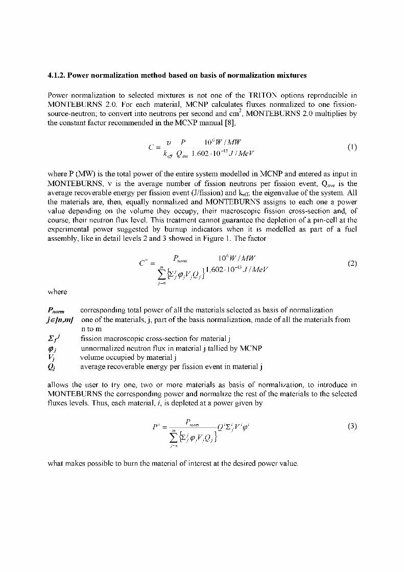
Power normalization to selected mixtures is not one of the TRITÓN options reproducible in MONTEBURNS 2.0. For each material, MCNP calculates fluxes normalized to one fission-source-neutron; to convert into neutrons per second and cm , MONTEBURNS 2.0 multiplies by the constant factor recommended in the MCNP manual [8],

_y P 106W/MW

~'K^Qave 1-602 -W^J/MeV

where P (MW) is the total power of the entire system modelled in MCNP and entered as input in MONTEBURNS, v is the average number of fission neutrons per fission event, Qave is the average recoverable energy per fission event (J/fission) and keff, the eigenvalue of the system. All the materials are, then, equally normalized and MONTEBURNS assigns to each one a power valué depending on the volume they occupy, their macroscopic fission cross-section and, of course, their neutrón flux level. This treatment cannot guarantee the depletion of a pin-cell at the experimental power suggested by burnup indicators when it is modelled as part of a fuel assembly, like in detail levéis 2 and 3 showed in Figure 1. The factor

Pnnm 106W/MW

\.602-\0~13J/MeV s~i norm ' fO\ ^ ~~^~ " i «cno I A - 1 3 * , * , ,r yZ>

where

Pnorm corresponding total power of all the materials selected as basis of normalization je[n,m] one of the materials, j , part of the basis normalization, made of all the materials from

nto m ZfJ fission macroscopic cross-section for material j (Pj unnormalized neutrón flux in material j tallied by MCNP Vj volume occupied by material j Qj average recoverable energy per fission event in material j

allows the user to try one, two or more materials as basis of normalization, to introduce in MONTEBURNS the corresponding power and normalize the rest of the materials to the selected fluxes levéis. Thus, each material, i, is depleted at a power given by

P'= — Q"L'fV'<p' (3) r i

what makes possible to burn the material of interest at the desired power valué.

4.1.3. Temperature distributions of the burning materials within modeled geometries

MONTEBURNS 2.0 works only one list of isotopes associated with a selected cross-sections library that applies to all burning materials. As a consequence, all the materials evolve at the temperature at which the selected library was generated and it is not possible to draw any temperature distribution followed by the materials. Our MONTEBURNS 2.0 versión works with different libraries in order to account for the different temperatures of the materials. In our case, two continuous-energy ACE format data libraries generated using NJOY-99.259 with 0.01 fractional reconstruction tolerance were used, on the one hand, based on ENDF/B-VII evaluation, on the other, based on JEFF-3.1.1 [9]. The prepared libraries include a total of 432 nuclides at 6 temperatures, but given the temperature conditions of our problem, only isotopes at 600K and 900K, for moderator and fuel respectively, were necessary.

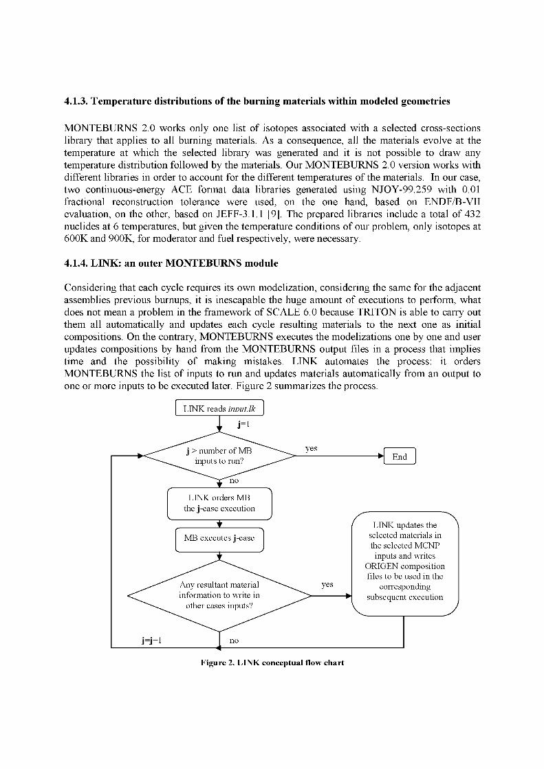
4.1.4. LINK: an outer MONTEBURNS module

Considering that each cycle requires its own modelization, considering the same for the adjacent assemblies previous burnups, it is inescapable the huge amount of executions to perform, what does not mean a problem in the framework of SCALE 6.0 because TRITÓN is able to carry out them all automatically and updates each cycle resulting materials to the next one as initial compositions. On the contrary, MONTEBURNS executes the modelizations one by one and user updates compositions by hand from the MONTEBURNS output files in a process that implies time and the possibility of making mistakes. LINK automates the process: it orders MONTEBURNS the list of inputs to run and updates materials automatically from an output to one or more inputs to be executed later. Figure 2 summarizes the process.

LINK updates the selected materials in the selected MCNP

inputs and writes ORIGEN composition files to be used in the

corresponding subsequent execution

Figure 2. LINK conceptual flow chart

5. RESULTS FOR VANDELLOS II CASE

With the purpose of validating our normalization methodology, cycles 7-11 modelization series were executed with TRITÓN (T), MONTEBURNS 2.0 (MB), MONTEBURNS 2.0 and MCNP-ACAB (only for level 1 geometrical detail) both including the new normalization capability (MBP and MAP, respectively).

TRITÓN calculations were performed with the SCALE 44-group cross-section library based on ENDF/B-V data and following the two-dimensional depletion sequence, which calis NEWT as transport code, ORIGEN-S as depletion code and NITAWL as cross-section processor.

MONTEBURNS versions and MCNP-ACAB [10] included the library-at-temperature selection option and were executed as part of our linking code functions, emulating, then, TRITÓN execution flow.

For MONTEBURNS 2.0 executions, processed librarles at 600 K and 900K based on ENDF/B-VII, as explained in subsection 3.1.3, were chosen. PWRU ORIGEN library was used.

For MCNP-ACAB, calculations are performed with the same processed libraries at 600 K and 900K based on ENDF/B-VII, and for the rest of reactions and the rest of nuclides not included in the MCNP library, but considered in ACAB code, the multigroup activation cross-section library EAF2007 collapsed with the MCNP flux, is used. For nuclides with cross-sections leading to meta stable states, (n,y-M) and (n, 2n-M), a branching ratio is used to update the ACAB cross-section library from total one-group MCNP valúes. This ratio is the same as in the activation cross-section library.

Before analyzing our results, it is mandatory to insist on the main difference between MB and MBP/MAP versions regarding to the present problem. Whereas original versión normalizes all the defined materials fluxes to averaged over the entire system magnitudes, our versión considers only those referred to materials forming the selected basis of normalization, in this case, E58-88 sample material.

LINK coordinated the executions of all the mentioned levéis of geometrical detail. Each isotope density (g/cc) in material of interest is calculated from the corresponding MONTEBURNS 2.0 outputs and compared to TRITÓN equivalent modelizations results. As shown in Table II, there is a better agreement between our updated MBP versión and TRITÓN than between original MONTEBURNS 2.0 and TRITÓN results. This improvement is actually shght in Level 1 modelization, as expected, due to the presence of only one fissionable material: in this case, there is no qualitative difference between the traditional normalization method of MONTEBURNS and ours. Meaningful deviations arise in the comparisons referred to levéis 2 and 3. For level 2, it can be seen that this new methodology approaches more to TRITÓN results for almost all the actinides and a good number of the studied fission products. This improvement is not so clear for level 3 at this level of burnup; however, all our results are within the accepted deviation margins between codes and for those that are beyond them ( Am, Cm, Cs, Sm, Sm, Eu and 156Gd) we find difficulties to reproduce TRITÓN results for all the geometries and normalization methodologies.

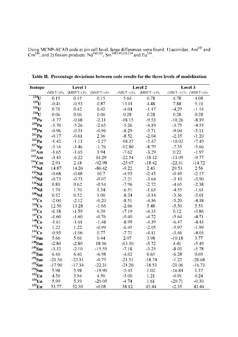
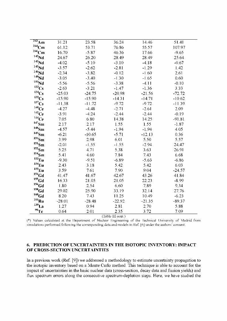
Using MCNP-ACAB code at pin cell level, large differences were found: 1) actinides: Am and ^ 2 4 4 J o \ f • J + -VTI 142,143 c 148,149,152,154 , c 154

Cm ; and 2) lission products: Nd , Sm and Eu

Table II. Percentage deviations between code results for the three levéis of modelization

Isotope Level 1 Level 2 Level 3 (MB/T-1)% (MBP/T-1)% (MAP/T-1)% (MB/T-1)% (MBP/T-1)% (MB/T-1)% (MBP/T-1)%

234U 2 3 5 u 2 3 6 u 2 3 8 u

2 3 8 p u

239Pu 2 4 0 p u

241Pu 2 4 2 p u

237Np 241 Am 243Am 244Cm 142Nd 143Nd 145Nd 146Nd 148Nd 150Nd 133Cs 134Cs 135Cs 137Cs 140Ce 142Ce 144Ce 147Sm 148Sm 149Sm 150Sm 151Sm 152Sm 154Sm 153Eu 154Eu 155Eu

0.15 -0.41 0.71 0.06 -1.77 -5.70 -0.96 -0.17 -1.42 -5.16 -1.65 -3.43 2.93 14.87 -0.68 -0.73 0.80 1.70 0.52 -2.00 12.56 -1.38 -1.60 -1.61 1.22 -0.95 5.66 -2.80 -3.32 6.40

-21.56 -17.90 5.98 4.50 5.99

53.77

0.15 -0.53 0.42 0.06 -0.68 -5.26 -0.33 -0.61 -1.13 -3.46 -1.65 -6.22 2.18 14.26 -0.68 -0.73 0.62 1.70 0.52 -2.12 13.28 -1.59 -1.60 -1.61 1.22 -1.06 5.66 -2.80 -2.10 6.40

-22.31 -17.34 5.98 3.94 5.39

52.30

0.15 0.87 0.42 0.06 -2.31 -2.65 -0.96 2.36 -2.27 -1.76 3.94

34.29 -92.98 -86.42

10.7 -0.07 -0.54 1.34 1.00 -0.20 -1.66 6.39 -0.76 -1.48 -0.99 0.77 0.44 18.36 -15.55 -6.98 -0.79

-22.31 -19.90 4.50

-20.05 -0.08

5.64 13.01 -4.04 0.28

-18.15 -5.26 -8.29 -8.52

-18.37 -12.80 -7.62

-22.54 -25.07 -9.22 -4.93 -7.21 -7.96 -6.51 -8.24 -8.51 -2.66 -7.19 -9.40 -8.99 -6.45 -7.71 2.07

-13.30 -7.18 -4.62

-21.51 -21.20 -5.43 -5.00 -4.74 38.12

0.78 4.48 -1.17 0.28 -9.53 -4.19 -5.71 -2.04 -5.47 -8.79 -3.29

-18.12 -18.42 2.43 -2.45 -3.64 -2.72 -1.63 -3.14 -4.36 5.48 -4.33 -4.72 -4.39 -2.05 -4.11 3.98 -5.72 -3.25 0.65

-18.74 -18.53 1.02 1.21 1.61

43.44

4.78 7.88 -4,29 0.28

-10.26 -3.75 -9.04 -2.35

-10.02 -7.55 0.22

-13.09 -22.31 29.53 -0.49 -3.10 -4.65 -4.55 -3.36 -5.20 -5.50 0.12 -5.64 -6.47 -5.97 -3.46

-10.18 4.41 -8.03 -6.28 -1.22

-21.06 -16.84 -0.91

-20.71 -2.35

4.08 5.10 -1.14 0.28 -8.39 -4.55 -5.11 -1.20 -7.49 -5.66 -1.97 -9.77

-14.72 2.56 -2.17 -3,90 -2.38 -1.61 -3.01 -4.38 5.53 -3.86 -4.71 -4.43 -1.99 -4.03 3.77 -5.49 -5.78 0.69

-20.68 -16.73 1.37 0.24 -0.30 43.44

154Gd 155Gd 156Gd 158Gd 160Gd 106Ru 139La " T e

7.16 42.30 6.40 12.75 25.71 -1.98 0.48 -1.06

6.68 41.06 6.23 11.98 25.45 -2.09 0.48 -1.22

0.15 0.87 0.42 0.06 -2.31 -2.65 -0.96 2.36

-5.51 28.43 -13.66 -5.74 9.33

-14.08 -7.17 -8.13

1.33 32.97 -2.36 3.20 18.26 -7.17 -2.71 -4.45

-3.12 37.72 0.02

28.19 -6.63 1.27

15.71 -13.12

0.86 33.39 -2.24 4.54 18.98 -6.97 -2.63 -4.16

(Table II cont.)

Table II assures us we have developed a valid methodology of reproducing measured isotopic compositions by normalizing fluxes and powers according to measured or reported power in the material of interest.

Since calculating measured compositions is the final objective of any depletion code, a validation exercise has to be done. LINK-MBP and LINK-MB results for Vandellós II eyeles 7-11 are compared to measured valúes in order to determine the quality of their methodologies in isotopic prediction calculations. Table III shows the simulated to experimental deviation percentage provided by both codes and TRITÓN in terms of [g/g U-238] % for each isotope at 1101 days of cooling from the end of the 11 eyele, in the level 3 modelization scheme. Series were executed in MB and MBP twice, first, using prepared libraries at 600 K and 900 K based on ENDF/B-VII, as mentioned before, and at 575 K and 900 K based on JEFF-3.1.1, later. This way, we ¿Ilústrate the clear dependence of a code result with the selected nuclear data library. As can be seen, in general, calculated isotopic abundances are within the accepted deviation margins. There are

241 243 244 Cm , fission-produets: Nd , 134 Cs1J", Cs 135 Gd 154 isotopes (actinides: Am , Am , Cm Gd , Ru ), however, for which no code is able to reproduce measured quantities under the 10% of deviation. We point out the reduction on deviation percentages provided by our linking methodology found for some fission products (see Cm144, Cs134, Ru ) in comparison with TRITÓN.

144 Ce1^, Sm 151 Sm152, Eu155 and

Table III. Comparison (C/E-l)*100% between different codes with measured valúes for sample E58-88 at 1101 days from discharge

Isotope 234U 2 3 5 u 2 3 6 u

2 3 8 p u

239Pu 2 4 0 p u

241Pu 2 4 2 p u

237Np 241Am

MB ENDF/B-VII

8.76 3.24 6.14 -9.97 -2.68 -1.53 -3.06 -2.12 -9.23 24.21

JEFF-3.1.1 7.32 3.24 5.52 -3.10 -3.50 0.59 -3.32 -3.03 -6.84 18.10

MBP ENDF/B-VII

8.04 0.58 7.39 -8.10 -3.50 2.72 -1.92 0.64 -7.37 21.50

JEFF-3.1.1 6.60 0.18 6.14 -2.47 -2.13 6.26 -3.95 1.25 -3.93 15.39

TRITÓN (*) ENDF/B-V 44-G

4.09 -4.03 8.94 0.60 1.39 8.56 -0.45 9.09 -1.54 24.29

243 A

Am Cm

246Cm 142Nd 143Nd 145Nd 146Nd 148Nd 150Nd 133Cs 134Cs 135Cs 137Cs 140Ce 142Ce 144Ce 147Sm 148Sm 149Sm 150Sm 151Sm 152Sm 154Sm 153Eu 154Eu 155Eu 154Gd 155Gd 156Gd 158Gd 160Gd 106Ru 139T

La 99rr

Te

31.21 61.12 16.70 24.67 -4.02 -3.57 -2.34 -3.05 -5.56 -2.63

-25.03 -15.90 -11.38 -4.27 -3.91 7.05 2.17 -4.57 -6.21 3.99 -2.01 5.25 5.41 -9.30 2.43 3.59

41.47 16.33 1.80

29.02 8.20

-28.01 1.27 0.64

23.58 53.71 -5.87 26.20 -5.10 -2.62 -3.82 -3.40 -5.56 -3.21

-24.75 -15.90 -11.72 -4.48 -4.24 6.80 2.17 -5.44

-10.65 2.98 -1.55 4.71 4.60 -9.51 3.18 7.61

41.67 21.05 2.54

25.90 7.43

-28.48 0.94 2.01

36.24 76.86 46.36 28.49 -3.10 -2.81 -0.12 -1.30 -3.38 -1.47

-20.98 -14.31 -9.72 -2.71 -2.44 14.38 1.55 -1.94 -5.71 6.01 -1.55 5.38 7.84 -6.89 5.42 7.90

42.67 21.05 6.60

33.19 11.25 -22.92 2.81 2.35

14.46 55.57 17.66 28.49 -4.18 -1.29 -1.60 -1.65 -4.11 -1.36

-21.56 -14.71 -9.72 -2.61 -2.44 14.25 1.55 -1.94

-12.13 5.50 -2.94 3.63 7.43 -5.63 5.42 9.04

43.26 22.23 7.89

32.14 10.49

-21.35 2.70 3.72

51.41 107.97 -9.65 25.64 -0.67 1.42 2.61 0.60 -0.10 3.33

-72.72 -10.62 -11.39 2.09 -0.19

-91.81 -1.87 4.05 0.36 5.57

24.47 26.91 6.68 -6.86 6.03

-24.57 41.84 -8.99 9.34

27.76 -6.23

-89.37 5.88 7.09

(Table III cont.) (*) Valúes calculated at the Department of Nuclear Engineering of the Technical University of Madrid from simulations performed following the corresponding data and models in Ref. [6] under the authors' consent.

6. PREDICTION OF UNCERTAEYTIES IN THE ISOTOPIC EWENTORY: IMPACT OF CROSS-SECTION UNCERTAEYTIES

In a previous work (Ref. [9]) we addressed a methodology to estímate uncertainty propagation to the isotopic inventory based on a Monte Cario method. This technique is able to account for the impact of uncertainties in the basic nuclear data (cross-section, decay data and fission yields) and flux spectrum errors along the consecutive spectrum-depletion steps. Here, we have studied the

impact of cross-section uncertainties in the actinides for the Phase-IB and Vandellós pin-cell presented in the previous sections.

Basically, the method is based on two steps. In a first step, a coupled neutron-depletion calculation is carried out only once, taken the best-estimated valúes for neutrón spectra. That is, when solving the transport equation to calcúlate the flux distribution for each time step, ñor uncertainties in the input parameters ñor statistical fluctuations are taken into account. This is called the best-estimated multi-step calculation. In a second step, the uncertainty analysis to evalúate the influence of the uncertainties in cross-sections involved in the transmutation process on the isotopic inventory is accomplished by the ACAB code. It performs a simultaneous random sampling of the probability density functions (PDF) of all those cross-sections. Then, ACAB computes the isotopic concentrations at the end of each burn step, taking the fluxes halfway through each burn step determined in the best-estimated calculation. In this way, only the depletion calculations are repeated or run many times. A statistical analysis of the results allows assessing the uncertainties in the calculated densities.

•

Best-estimated calculation •

<% = { % , ..., tfp,..., o-m0>

Uncertainty calculation

PDF

Ti D> rn c

ACAB step 1

/ T * % j

•,

0,

ACAB step 2

i/*T"N^

«CNP

U *2

1 " MCNP

ti

- ~ \ ü E ti E

» 1 i i* ™ "í^stoiy VÑ!

\j__y history M

A-/ Y am

^Ji istoryW

V L / htstory M

/ v

A* %

Buriiup

• Buniup

N Í ^ - t N , , ..

OUTPUT

•i > 1 y

. N¡ N„)

Sample of M vectors |.V| of isotopic concentrations

P D F

r\N' /AN \

1 1 ^̂ ~ <N¡> N ¡ M NB5

Figure 3. Monte Cario method scheme implemented in MCNP-ACAB system to propágate uncertainties in final concentrations.

In Table IV, we have applied the Monte Cario formulation to estímate the errors in the actinide inventory for the two Burnup problems defined above. The actinides under consideration are the ones specified as important in the benchmark. And, the uncertainties in cross-sections are taken from EAF2007/UN.

Taking into account the differences in those burnup calculations, it can be concluded that:

1) In general, for actinides and fission products, the uncertainty throughout irradiation period raises.

2) It can be seen that for major actinides in Phase-IB the uncertainty remains below 2% and in the Vandellos case this uncertainty increases up to 7.6% for Pu240. Larger uncertainties are predicted for minor actinides (e.g. in the Vandellos case, 14.5% for 246Cm)

3) In the case of fission products, cross section uncertainties contribute more largely. In the Vandellos case, the uncertainty in fission products due to fission yields remains below 10% (e.g. 9.93% for Ru106). Finally, activation cross-section uncertainties justify the significant relative errors shown in Table IV for Sml49, Eu and Gd isotopes.

At this respect, we have compared different source of uncertainties for activation cross-sections data (e.g. SCALE6.0/COVA-44G [11]). And, it can be conclude that EAF2007/UN ís very conservative. For instance, in the Sm149 prediction, the main pathway to the formation of this isotope is: fission—• Pr149 —• Nd149 —• Pm149 —• Sm149. The main sensitivity to Sm149 prediction is due to Sm149(n,y) reaction (about 1% change in Sml49 concentration due to a change of 1% in this reaction). EAF2007/UN assumes a relative error of -15% for this reaction against a 2% of relative error predi cted using SCALE6.0/COVA-44G For europium and gadolinium isotopes discrepantes between EAF2007/UN and SCALE6.0/COVA-44Gare also found.

Table IV. MCNP-ACAB calculated uncertainties in actinides due to cross-section uncertainties at

1) OECD/NEA Burnup Credit Benchmark. Phase-IB (CÁSEA- 27.35 GWd/TU)

Isotope

234U 2 3 5 u 2 3 6 u 2 3 8 u

2 3 8 p u

239Pu 2 4 0 p u

241Pu 2 4 2 p u

241 A

Am 243 A

Am 237Np

Reí, . Err. (%) Cross Section

1.7 0.49 0.37 0.06 1.08 0.96 1.39 1.17 1.13 1.15 2.31 0.49

Isotope

99rr

Te 95Mo 101Ru 103Rh 109Ag 133Cs

143Nd 145Nd 147Sm 149Sm 150Sm 151Sm 152Sm 153Eu 155Gd

Reí . Err. (%) Cross Section

0.36 0.35 0.38 1.15 1.36 0.38 0.39 0.39 0.69 9.70 0.62 1.74 1.05 3.01 1.58

2) Pin-cell level Vandellós II Reactor (42.5 GWd/TU)

Isotope Reí. Err. (%) Isotope Reí. Err. (%) Reí. Err. (%) Cross Section Cross Section Fission Yield

2 3 4 u 2 3 5 u 2 3 6 u 2 3 8 u

2 3 8 p u

239Pu 2 4 0 p u

241Pu 2 4 2 p u

237Np 2 4 1Am 243 A

Am 2 4 4Cm 2 4 6Cm

3.58 0.98 0.87 0.22 2.29 3.85 7.64 5.09 2.56 2.02 4.41 6.38 6.41 14.5

133Cs 134Cs 135Cs 137Cs 140Ce 142Ce 144Ce

147Sm 148Sm 149Sm 150Sm 151Sm 152Sm 154Sm 153Eu 154Eu 155Eu 154Gd 155Gd 156Gd 158Gd 160Gd 106Ru 139La

99Tc

0.79 5.59 2.27 0.76 0.72 0.72 1.15 2.94 2.73 14.8 1.85 3.16 3.85 0.84 13.4 23.0 36.8 17.5 36.5 10.2 14.4 1.42 1.19 0.73 0.93

2.53 1.54 2.69 3.27 3.64 2.83 6.00 2.67 1.89 5.61 2.72 6.16 3.52 3.24 1.72 1.43 3.16 1.30 3.13 2.00 3.72 7.50 9.93 3.09 2.93

7. CONCLUSIONS

In order to reproduce the isotopic content of a real problem, Vandellós II reactor cycles 7-11 in this case, we have corrected MONTEBURNS 2.0 feed capability and developed three tools: LINK, to automate executions; the capability of selecting libraries at different temperatures; and, finally, a new flux normalization method to reproduce exactly a sample of interest measured burnup. Since this capability is inspired by SCALE 6.0 TRITÓN module, previously benchmarked with other reviewed codes, the same reported data has been modeled for three

levéis of geometrical detail. Comparisons between codes results show a good agreement at pin-cell level, as expected, but MONTEBURNS 2.0 corrected and updated versión approaches more to TRITÓN valúes at higher levéis for major actinides and some fission products. Compared to experimental valúes, though, any improvement is disguised by the dependence of the results to the used library. Nevertheless, MONTEBURNS 2.0 including our improvements calculates compositions within the same order of deviation than a reference code like SCALE 6.0 TRITÓN. It is also remarkable the accuracy achieved in the prediction of some fission products in comparison with TRITÓN, what suggests that the linking methodology implemented in LINK is in the right direction. However, deeper studies have to be carried out to identify the origin of the deviations and to try to reduce them. Corrected and updated MONTEBURNS 2.0 capabilities and isotopic prediction power has to be tested at higher burnup levéis. These validation exercises will determine whether our improvements are in the right direction or not. MCNP-ACAB will be then applied to obtain final uncertainties from its propagation as explained, but it is foreseeable an increasing in these uncertainties with an increasing in the sample burnup. Special attention will be paid to fission products and we will study the impact of fission yields and decay data uncertainties, not considered in the present paper, on isotopic prediction calculations, what will help us to determine their independent importance compared to cross-section uncertainties and their importance in the final uncertainty as a whole.

ACKNOWLEDGMENTS

We thank the Spanish Nuclear Safety Council (CSN, Consejo de Seguridad Nuclear) for providing us with all the required information related to our case of study and sponsoring this work in the framework of the agreement P090531725 on Burnup Credit Criticality Safety. We thank specially Consuelo Alejano and J.M.Conde, who made easy the communication with Germina Has and lan C. Gauld, of the Oak Ridge National Laboratory, authors of the report Analisys of Experimental Datafor High Burnup PWR Spent Fuel Isotopic Validation- Vandellós II Reactor. Finally, the authors would like to thank Germina Has and lan C. Gauld for allowing us to use part of their Vandellós II reactor cycles 7-11 inspiring modelizations and results as reference for the present paper, as well as for their patient assistance and guidance.

REFERENCES

1. AEA Technology, WIMSD5: Deterministic Multigroup Reactor Lattice Calculations, distributed by the NEADatabank, 2004

2. Jaako Leppánen, PSG2/Serpent: a Continous-energy Monte Cario Reactor Physics Burnup Calculation Code (User's Manual), May 2010

3. Mark D. DeHart, TRITÓN: a Two-Dimensional Transport and Depletion Module For Characterization of Spent Nuclear Fuel, ORNLTM-2005/39 Versión 6 Vol. I. Sect. TI, January 2009

4. Poston D. I , Trellue H.R., User's Manual, Versión 2.0 for MONTEBURNS Versión LO, LA-UR-99-4999, September 1, 1999

5. DeHart M.D., Bady M.C., Parks C.V, OECD/NEA Burnup Credit Calculational Criticality Benchmark Phase I-B Results, ORNL-6901, Oak Ridge National Laboratory, June 1996

6. Ref. H.U. Zwicky, J. Low, M. Granfors, C. Alejano, J.M. Conde, C. Casado, J. Sabater, M. Lloret, M. Quecedo, J.A. Gago, "Nuclide analysis in high burnup fuel samples irradiated in Vandellós 2", Journal of Nuclear Materials, Volume 402, Issue 1, 1 July 2010, pp. 60-73.

7. G Has and I. C. Gauld, Analysis of Experimental Datafor High Burnup PWR Spent Fuel Isotopic Validation - Vandellós IIReactor, NUREG/CR-7013 (ORNL/TM-2009/321), U.S. Nuclear Regulatory Commission Office of Nuclear Regulatory Research (2010, under publication).

8. X-5 Monte Cario Team. MCNP-A General Monte Cario N-Particle Transport Code, Versión 5- Los Alamos National Laboratory. April 24, 2003

9. T. Viitanen and J. Leppánen, Continuous-energy X-sec lib., radioactive decay, fission yield datafor SERPENT in ACE, NEA-1854 ZZ-SERPENT117-ACELIB

10. Nuria García-Herranz, Osear Cabellos, Javier Sanz, Jesús Juan, Jim C. Kuijper, "Propagation of statistical and nuclear data uncertainties in Monte Cario burn-up calculations", Annals of Nuclear Energy, Volume 35, Issue 4, April 2008, pp. 714-730

11. ZZ SCALE6.0/COVA-44Q 44-group cross section covariance matrix library extracted from SCALE6.0, USCD1236/02 Package. OECD/NEAData Bank.