Isotope distributionsThis exposition is based on:

• R. Martin Smith: Understanding Mass Spectra. A Basic Approach. Wiley, 2ndedition 2004. [S04]

• Exact masses and isotopic abundances can be found for example at http://www.sisweb.com/referenc/source/exactmaa.htm or http://education.

expasy.org/student_projects/isotopident/htdocs/motza.html

• IUPAC Compendium of Chemical Terminology - the Gold Book. http://

goldbook.iupac.org/ [GoldBook]

• Sebastian Bocker, Zzuzsanna Liptak: Efficient Mass Decomposition. ACMSymposium on Applied Computing, 2005. [BL05]

• Christian Huber, lectures given at Saarland University, 2005. [H05]

• Wikipedia: http://en.wikipedia.org/, http://de.wikipedia.org/10000

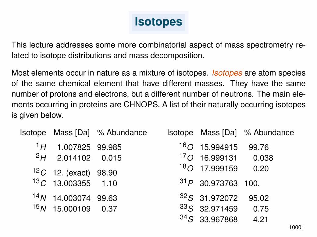
Isotopes

This lecture addresses some more combinatorial aspect of mass spectrometry re-lated to isotope distributions and mass decomposition.

Most elements occur in nature as a mixture of isotopes. Isotopes are atom speciesof the same chemical element that have different masses. They have the samenumber of protons and electrons, but a different number of neutrons. The main ele-ments occurring in proteins are CHNOPS. A list of their naturally occurring isotopesis given below.

Isotope Mass [Da] % Abundance1H 1.007825 99.9852H 2.014102 0.015

12C 12. (exact) 98.9013C 13.003355 1.1014N 14.003074 99.6315N 15.000109 0.37

Isotope Mass [Da] % Abundance16O 15.994915 99.7617O 16.999131 0.03818O 17.999159 0.2031P 30.973763 100.32S 31.972072 95.0233S 32.971459 0.7534S 33.967868 4.21

10001

Isotopes (2)

Note that the lightest isotope is also the most abundant one for these elements.Here is a list of the heavy isotopes, sorted by abundance:

Isotope Mass [Da] % Abundance34S 33.967868 4.2113C 13.003355 1.1033S 32.971459 0.7515N 15.000109 0.3718O 17.999159 0.2017O 16.999131 0.038

2H 2.014102 0.015

We see that sulfur has a big impact on the isotope distribution. But it is not alwayspresent in a peptide (only the amino acids Cystein or Methionin contain sulfur).Apart from that, 13C is most abundant, followed by 15N. These isotopes lead to“+1” peaks. The heavy isotopes 18O and 34S lead to “+2” peaks. Note that 17O and2H are very rare.

10002

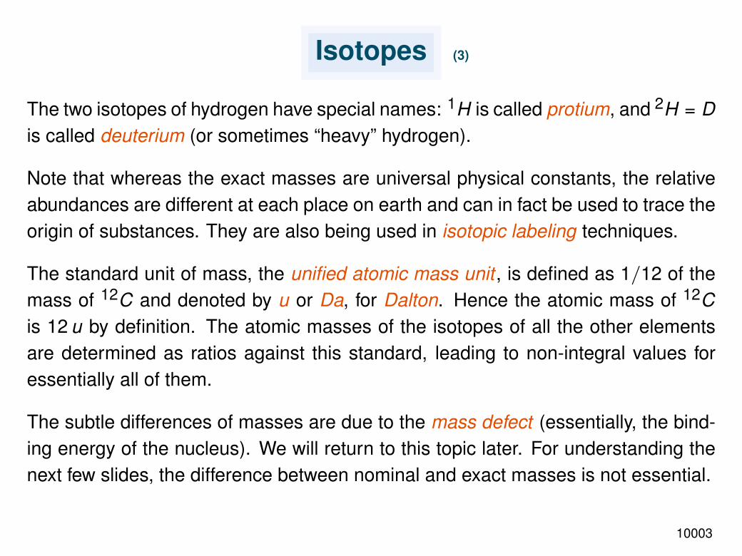
Isotopes (3)

The two isotopes of hydrogen have special names: 1H is called protium, and 2H = Dis called deuterium (or sometimes “heavy” hydrogen).

Note that whereas the exact masses are universal physical constants, the relativeabundances are different at each place on earth and can in fact be used to trace theorigin of substances. They are also being used in isotopic labeling techniques.

The standard unit of mass, the unified atomic mass unit , is defined as 1/12 of themass of 12C and denoted by u or Da, for Dalton. Hence the atomic mass of 12Cis 12 u by definition. The atomic masses of the isotopes of all the other elementsare determined as ratios against this standard, leading to non-integral values foressentially all of them.

The subtle differences of masses are due to the mass defect (essentially, the bind-ing energy of the nucleus). We will return to this topic later. For understanding thenext few slides, the difference between nominal and exact masses is not essential.

10003

Isotopes (4)

The average atomic mass (also called the average atomic weight or just atomicweight) of an element is defined as the weighted average of the masses of all itsnaturally occurring stable isotopes.

For example, the average atomic mass of carbon is calculated as

(98.9% ∗ 12.0 + 1.1% ∗ 13.003355)100%

.= 12.011

For most purposes such as weighing out bulk chemicals only the average molecularmass is relevant since what one is weighing is a statistical distribution of varyingisotopic compositions.

The monoisotopic mass is the sum of the masses of the atoms in a molecule usingthe principle isotope mass of each atom instead of the isotope averaged atomicmass and is most often used in mass spectrometry. The monoisotopic mass ofcarbon is 12.

10004

Isotopes (5)

According to the [GoldBook] the principal ion in mass spectrometry is a molecular orfragment ion which is made up of the most abundant isotopes of each of its atomicconstituents.

Sometimes compounds are used that have been artificially isotopically enrichedin one or more positions, for example CH3

13CH3 or CH2D2. In these cases theprincipal ion may be defined by treating the heavy isotopes as new atomic species.Thus, in the above two examples, the principal ions would have masses 31 (not 30)and 18 (not 16), respectively.

In the same vein, the monoisotopic mass spectrum is defined as a spectrum con-taining only ions made up of the principal isotopes of atoms making up the originalmolecule.

You will see that the monoisotopic mass is sometimes defined using the lightestisotope. In most cases the distinction between ”principle” and ”lightest” isotopeis non-existent, but there is a difference for some elements, for example iron andargon.

10005

Isotopic distributions

The mass spectral peak representing the monoisotopic mass is not always the mostabundant isotopic peak in a spectrum – although it stems from the most abundantisotope of each atom type.

This is due to the fact that as the number of atoms in a molecule increases theprobability of the entire molecule containing at least one heavy isotope increases.For example, if there are 100 carbon atoms in a molecule, each of which has anapproximately 1% chance of being a heavy isotope, then the whole molecule is notunlikely to contain at least one heavy isotope.

The monoisotopic peak is sometimes not observable due to two primary reasons.

• The monoisotopic peak may not be resolved from the other isotopic peaks. Inthis case only the average molecular mass may be observed.

• Even if the isotopic peaks are resolved, the monoisotopic peak may be belowthe noise level and heavy isotopomers may dominate completely.

10006

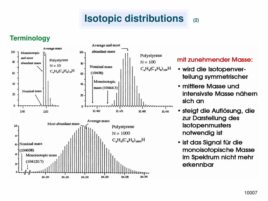
Isotopic distributions (2)

Terminology

10007

Isotopic distributions (3)

Example:

10008

Isotopic distributions (4)

To summarize: Learn to distinguish the following concepts!

• nominal mass

• monoisotopic mass

• most abundant mass

• average mass

10009

Isotopic distributions (5)

Example: Isotopic distribution of human myoglobin

Screen shot: http://education.expasy.org/student_projects/isotopident/10010

Isotopic distributions (6)

A basic computational task is:

• Given an ion whose atomic composition is known, how can we compute itsisotopic distribution?

We will ignore the mass defects for a moment. It is convenient to number the peaksby their number of additional mass units, starting with zero for the lowest isotopicpeak. We can call this the isotopic rank .

Let E be a chemical element. Let πE [i ] denote the probability of the isotope of Ehaving i additional mass units. Thus the relative intensities of the isotopic peaks fora single atom of element E are (πE [0],πE [1],πE [2], ...,πE [kE ]). Here kE denotesthe isotopic rank of the heaviest isotope occurring in nature. We have πE [`] = 0 for` > k .

For example carbon has πC[0] = 98.9% = 0.989 (isotope 12C) and πC[1] = 1.1% =0.011 (isotope 13C).

10011

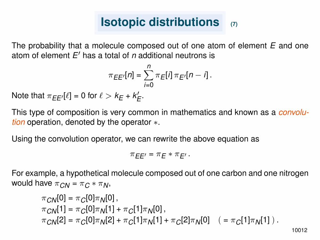
Isotopic distributions (7)

The probability that a molecule composed out of one atom of element E and oneatom of element E ′ has a total of n additional neutrons is

πEE ′[n] =n∑

i=0πE [i ]πE ′[n − i ] .

Note that πEE ′[`] = 0 for ` > kE + k ′E .

This type of composition is very common in mathematics and known as a convolu-tion operation, denoted by the operator ∗.

Using the convolution operator, we can rewrite the above equation as

πEE ′ = πE ∗ πE ′ .

For example, a hypothetical molecule composed out of one carbon and one nitrogenwould have πCN = πC ∗ πN ,

πCN [0] = πC[0]πN [0] ,πCN [1] = πC[0]πN [1] + πC[1]πN [0] ,πCN [2] = πC[0]πN [2] + πC[1]πN [1] + πC[2]πN [0]

(= πC[1]πN [1]

).

10012

Isotopic distributions (8)

Clearly the same type of formula applies if we compose a larger molecule out ofsmaller molecules or single atoms. Molecules have isotopic distributions just likeelements.

For simplicity, let us define convolution powers. Let ρ1 := ρ and ρn := ρn−1 ∗ ρ, forany isotopic distribution ρ. Moreover, it is natural to define ρ0 by ρ0[0] = 1, ρ0[`] = 0for ` > 0. This way, ρ0 will act as neutral element with respect to the convolutionoperator ∗, as expected.

Then the isotopic distribution of a molecule with the chemical formula E1n1· · ·E`n`,

composed out of the elements E1, ... , E`, can be calculated as

πE1n1···E`n`

= πn1E1∗ ... ∗ πn`

E`.

10013

Isotopic distributions (9)

This immediately leads to an algorithm. for computing the isotopic distribution of amolecule.

Now let us estimate the running time for computing πn1E1∗ ... ∗ πnl

El.

• The number of convolution operations is n1 + ... + nl − 1, which is linear in thenumber of atoms.

• Each convolution operation involves a summation for each π[i ]. If the highestisotopic rank for E is kE , then the highest isotopic rank for En is kEn. Again,this in linear in the number of atoms.

We can improve on both of these factors.

Do you see how?

10014

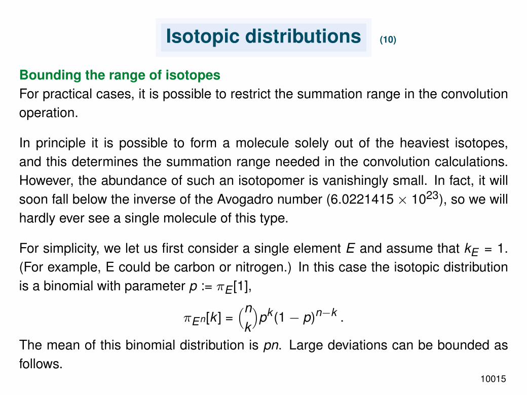
Isotopic distributions (10)

Bounding the range of isotopesFor practical cases, it is possible to restrict the summation range in the convolutionoperation.

In principle it is possible to form a molecule solely out of the heaviest isotopes,and this determines the summation range needed in the convolution calculations.However, the abundance of such an isotopomer is vanishingly small. In fact, it willsoon fall below the inverse of the Avogadro number (6.0221415× 1023), so we willhardly ever see a single molecule of this type.

For simplicity, we let us first consider a single element E and assume that kE = 1.(For example, E could be carbon or nitrogen.) In this case the isotopic distributionis a binomial with parameter p := πE [1],

πEn[k ] =(nk

)pk (1− p)n−k .

The mean of this binomial distribution is pn. Large deviations can be bounded asfollows.

10015

Isotopic distributions (11)

We use the upper bound for binomial coefficients

(nk

)≤(ne

k

)k.

For k ≥ 3pn (that is, k three times larger than expected) we get

(nk

)pk ≤

(nep2pn

)k=(e

3

)k.

and hencen∑

`≥3pn

(nk

)pk (1− p)n−k ≤

n∑`≥3pn

(e3

)k= O

((e3

)3pn)

= o(1) .

While 3pn is still linear in n, it is much smaller – in practice one can usually restrictthe calculations to less than 10 isotopic variants for peptides.

Fortunately, if it turns out that the chosen range was too small, we can detect thisafterwards because the probabilities will no longer add up to 1. (Exercise: Explainwhy.) Thus we even have an ‘a posteriori error estimate’.

10016

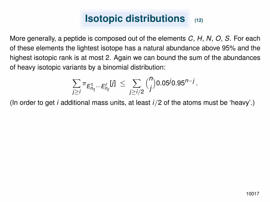
Isotopic distributions (12)

More generally, a peptide is composed out of the elements C, H, N, O, S. For eachof these elements the lightest isotope has a natural abundance above 95% and thehighest isotopic rank is at most 2. Again we can bound the sum of the abundancesof heavy isotopic variants by a binomial distribution:∑

j≥iπE1

n1···E`n`

[j ] ≤∑

j≥i/2

(nj

)0.05j0.95n−j .

(In order to get i additional mass units, at least i/2 of the atoms must be ‘heavy’.)

10017

Isotopic distributions (13)

Computing convolution powers by iterated squaringThere is another trick which can be used to save the number of convolutions neededto calculate the n-th convolution power πn of an elemental isotope distribution.

Observe that just like for any associative operation ∗, the convolution powers satisfy

π2n = πn ∗ πn .

In general, n is not a power of two, so let (bj , bj−1, ... , b0) be the bits of the binaryrepresentation of n, that is,

n =j∑`=0

b`2` = bj2

j + bj−12j−1 + · · · + b020 .

Then we can compute πn as follows:

πn = π∑

j 2jbj =∏jπ2jbj = πbj2j

∗ πbj−12j−1∗ · · · ∗ πb020

,

where the∏

is of course meant with respect to ∗. The total number of convolutionsneeded for this calculation is only O(log n).

10018

Isotopic distributions (14)

To summarize: The first k + 1 abundances πEn

1 ···En``

[i ], i = 0, ... , k , of the isotopic

distribution of a molecule En11 · · ·E

n`` can be computed in O(`k log n) time and O(`k )

space, where n = n1 + ... + n`.

(Exercise: To test your understanding, check how these resource bounds followfrom what has been said above.)

10019

Mass decomposition

A related question is:

• Given a peak mass, what can we say about the elemental composition of theion that generated it?

In most cases, one cannot obtain much information about the chemical structuralfrom just a single peak. The best we can hope for is to obtain the chemical formulawith isotopic information attached to it. In this sense, the total mass of an ion is de-composed into the masses of its constituents, hence the term mass decomposition.

10020

Mass decomposition (2)

This is formalized by the concept of a compomer [BL05].

We are given an alphabet Σ of size |Σ| = k , where each letter has a mass ai ,i = 1, ... , k . These letters can represent atom types, isotopes, or amino acids, ornucleotides. We assume that all masses are different, because otherwise we couldnever distinguish them anyway. Thus we can identify each letter with its mass, i. e.,Σ = {a1, ... , ak} ⊂ N. This is sometimes called a weighted alphabet .

The mass of a string s = s1 ... sn ∈ Σ∗ is defined as the sum of the masses of itsletters, i. e., mass(s) =

∑|s|i=1 si .

Formally, a compomer is an integer vector c = (c1, ... , ck ) ∈ (N0)k . Each cirepresents the number of occurrences of letter ai . The mass of a compomer ismass(c) :=

∑ki=1 ciai , as opposed to its length, |c| :=

∑ki=1 ci .

In short: A compomer tells us how many instances of an atomic species are presentin a molecule. We want to find all compomers whose mass is equal to the observedmass.

10021

Mass decomposition (3)

There a many more strings (molecules) than compomers, but the compomers arestill many.

For a string s = s1 ... sn ∈ Σ∗, we define comp(s) := (c1, ... , ck ), where ci :=#{j | sj = ai}. Then comp(s) is the compomer associated with s, and vice versa.

One can prove (exercise):

1. The number of strings associated with a compomer c = (c1, ... , ck ) is( |c|

c1,...,ck

)=

|c|!c1!···ck ! .

2. Given an integer n, the number of compomers c = (c1, ... , ck ) with |c| = n is(n+k−1

k−1

).

Thus a simple enumeration will not suffice for larger instances.

10022

Mass decomposition (4)

Using dynamic programming, we can solve the following problems efficiently(Σ: weighted alphabet, M: mass):

1. Existence problem: Decide whether a compomers c with mass(c) = M exists.

2. One Witness problem: Output a compomer c with mass(c) = M, if one exists.

3. All witnesses problem: Compute all compomers c with mass(c) = M.

10023

Mass decomposition (5)

The dynamic programming algorithm is a variation of the classical algorithm origi-nally introduced for the ‘Coin Change Problem’, originally due to Gilmore and Go-mory.

Given a query mass M, a two-dimensional Boolean table B of size kM is constructedsuch that

B[i , m] = 1 ⇐⇒ m is decomposable over {a1, ... , ai} .

The table can be computed with the following recursion:

B[1, m] = 1 ⇐⇒ m mod a1 = 0

and for i > 0,

B[i , m] =

B[i − 1, m] m < ai ,B[i − 1, m] ∨ B[i , m − ai ] otherwise .

The table is constructed up to mass M, and then a straight-forward backtrackingalgorithm computes all witnesses of M.

10024

Mass decomposition (6)

For the Existence and One Witness Problems, it suffices to construct a one-dimensional Boolean table A of size M, using the recursion A[0] = 1, A[m] = 0for 1 ≤ m < a1; and for m ≥ a1, A[m] = 1 if there exists an i with 1 ≤ i ≤ ksuch that A[m − ai ] = 1, and 0 otherwise. The construction time is O(kM) and onewitness c can be produced by backtracking in time proportional to |c|, which can bein the worst case 1

a1M. Of course, both of these problems can also be solved using

the full table B.

A variant computes γ(M), the number of decompositions of M, in the last row, wherethe entries are integers, using the recursion C[i , m] = C[i − 1, m] + C[i , m − ai ].

The running time for solving the All Witnesses Problem is O(kM) for the table con-struction, and O(γ(M) 1

a1M) for the computation of the witnesses (where γ(M) is the

size of the output set), while storage space is (O(kM).

10025

Mass decomposition (7)

The number of compomers is O(MΣ). (Exercise: why?) Depending on the massresolution, the results can be useful for M up to, say, 1000 Da, but in general onehas to take further criteria into account. (Figure from [BL].)

10026

Mass decomposition (8)

Example output from http://bibiserv.techfak.uni-bielefeld.de/decomp/

# imsdecomp 1.3# Copyright 2007,2008 Informatics for Mass Spectrometry group# at Bielefeld University## http://BiBiServ.TechFak.Uni-Bielefeld.DE/decomp/## precision: 4e-05# allowed error: 0.1 Da# mass mode: mono# modifiers: none# fixed modifications: none# variable modifications: none# alphabet (character, mass, integer mass):# H 1.007825 25196# C 12 300000# N 14.003074 350077# O 15.994915 399873# P 30.973761 774344# S 31.972071 799302# constraints: none# chemical plausibility check: off## Shown in parentheses after each decomposition:# - actual mass# - deviation from actual mass

10027

## mass 218.03 has 1626 decompositions (showing the best 100):H2 C6 N8 O2 (218.03007; +7.1384e-05)H8 C7 N1 O7 (218.03008; +7.6606e-05)H13 C2 N5 O1 P1 S2 (218.02991; -8.7014e-05)H139 O1 P2 (218.03012; +0.000117068)H19 C1 N1 O3 P3 S1 (218.02985; -0.000151322)H16 N3 O4 S3 (218.03029; +0.000293122)H5 C2 N9 O2 P1 (218.03038; +0.00038199)H11 C3 N2 O7 P1 (218.03039; +0.000387212)H10 C6 N4 O1 S2 (218.0296; -0.00039762)H16 C5 O3 P2 S1 (218.02954; -0.000461928)H16 C3 N3 P4 (218.02947; -0.000531458)H21 C2 N1 P1 S4 (218.02944; -0.000556018)H8 N7 O5 S1 (218.03076; +0.000762126)H14 C1 O10 S1 (218.03077; +0.000767348)H18 C5 O1 P4 (218.03081; +0.000811196)H13 C7 N2 P3 (218.02916; -0.000842064)H18 C6 S4 (218.02913; -0.000866624)H12 C8 N1 O2 S2 (218.03095; +0.000945034)H9 C1 N5 O6 P1 (218.02904; -0.000955442)H3 N12 O1 P1 (218.02904; -0.000960664)H21 C1 N1 O1 P5 (218.03112; +0.001121802)H10 C11 N1 P2 (218.02885; -0.00115267)H137 O3 S1 (218.02884; -0.001156056)H15 C4 N2 O2 P1 S2 (218.03126; +0.00125564)H6 C5 N4 O6 (218.02873; -0.001266048)C4 N11 O1 (218.02873; -0.00127127)H4 C8 N5 O3 (218.03141; +0.001414038)H17 C1 N1 O5 P1 S2 (218.02858; -0.001424446)

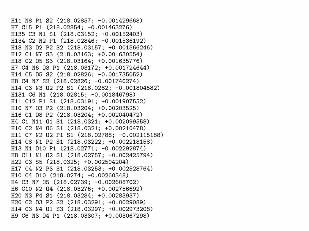
H11 N8 P1 S2 (218.02857; -0.001429668)H7 C15 P1 (218.02854; -0.001463276)H135 C3 N1 S1 (218.03152; +0.00152403)H134 C2 N2 P1 (218.02846; -0.001536192)H18 N3 O2 P2 S2 (218.03157; +0.001566246)H12 C1 N7 S3 (218.03163; +0.001630554)H18 C2 O5 S3 (218.03164; +0.001635776)H7 C4 N6 O3 P1 (218.03172; +0.001724644)H14 C5 O5 S2 (218.02826; -0.001735052)H8 C4 N7 S2 (218.02826; -0.001740274)H14 C3 N3 O2 P2 S1 (218.0282; -0.001804582)H131 C6 N1 (218.02815; -0.001846798)H11 C12 P1 S1 (218.03191; +0.001907552)H10 N7 O3 P2 (218.03204; +0.00203525)H16 C1 O8 P2 (218.03204; +0.002040472)H4 C1 N11 O1 S1 (218.0321; +0.002099558)H10 C2 N4 O6 S1 (218.0321; +0.00210478)H11 C7 N2 O2 P1 S1 (218.02788; -0.002115188)H14 C8 N1 P2 S1 (218.03222; +0.002218158)H13 N1 O10 P1 (218.02771; -0.002292874)H8 C11 N1 O2 S1 (218.02757; -0.002425794)H22 C3 S5 (218.0325; +0.002504204)H17 C4 N2 P3 S1 (218.03253; +0.002528764)H10 C4 O10 (218.0274; -0.00260348)H4 C3 N7 O5 (218.02739; -0.002608702)H6 C10 N2 O4 (218.03276; +0.002756692)H20 N3 P4 S1 (218.03284; +0.00283937)H20 C2 O3 P2 S2 (218.03291; +0.0029089)H14 C3 N4 O1 S3 (218.03297; +0.002973208)H9 C6 N3 O4 P1 (218.03307; +0.003067298)

H12 C3 N3 O4 S2 (218.02692; -0.003077706)H12 C1 N6 O1 P2 S1 (218.02685; -0.003147236)H18 N2 O3 P4 (218.02679; -0.003211544)H12 C2 N4 O4 P2 (218.03338; +0.003377904)H6 C3 N8 O2 S1 (218.03344; +0.003442212)H12 C4 N1 O7 S1 (218.03345; +0.003447434)H9 C5 N5 O1 P1 S1 (218.02654; -0.003457842)H15 C4 N1 O3 P3 (218.02648; -0.00352215)H20 C1 N2 P2 S3 (218.02638; -0.00361624)H15 N2 O7 P1 S1 (218.03376; +0.00375804)H6 C9 N4 O1 S1 (218.02623; -0.003768448)H12 C8 O3 P2 (218.02617; -0.003832756)H17 C5 N1 P1 S3 (218.02607; -0.003926846)H8 C2 N3 O9 (218.02605; -0.003946134)H2 C1 N10 O4 (218.02605; -0.003951356)H2 C11 N6 (218.03409; +0.004094124)H22 C2 O1 P4 S1 (218.03418; +0.004182024)H14 C9 S3 (218.02576; -0.004237452)H16 C5 N1 O2 S3 (218.03432; +0.004315862)H5 C7 N7 P1 (218.0344; +0.00440473)H11 C8 O5 P1 (218.03441; +0.004409952)H10 C1 N6 O3 S2 (218.02558; -0.00442036)H16 N2 O5 P2 S1 (218.02552; -0.004484668)H133 C3 O3 (218.02547; -0.004526884)H19 C1 N2 O2 P1 S3 (218.03463; +0.004626468)H8 C3 N8 P2 (218.03472; +0.004715336)H14 C4 N1 O5 P2 (218.03472; +0.004720558)H8 C5 N5 O3 S1 (218.03478; +0.004784866)H13 C4 N1 O5 P1 S1 (218.0252; -0.004795274)H7 C3 N8 P1 S1 (218.0252; -0.004800496)

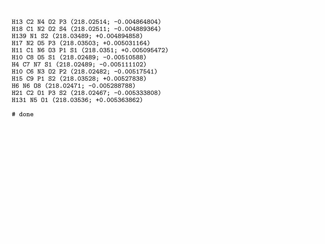
H13 C2 N4 O2 P3 (218.02514; -0.004864804)H18 C1 N2 O2 S4 (218.02511; -0.004889364)H139 N1 S2 (218.03489; +0.004894858)H17 N2 O5 P3 (218.03503; +0.005031164)H11 C1 N6 O3 P1 S1 (218.0351; +0.005095472)H10 C8 O5 S1 (218.02489; -0.00510588)H4 C7 N7 S1 (218.02489; -0.005111102)H10 C6 N3 O2 P2 (218.02482; -0.00517541)H15 C9 P1 S2 (218.03528; +0.00527838)H6 N6 O8 (218.02471; -0.005288788)H21 C2 O1 P3 S2 (218.02467; -0.005333808)H131 N5 O1 (218.03536; +0.005363862)

# done

Mass defect

The difference between the actual atomic mass of an isotope and the nearest inte-gral mass is called the mass defect . The size of the mass defect varies over thePeriodic Table. The mass defect is due to the binding energy of the nucleus:

http://de.wikipedia.org/w/index.php?title=Datei:Bindungsenergie_massenzahl.jpg10028

Mass defect (2)

The mass differences of light and heavy isotopes are also not exactly multiples ofthe atomic mass unit. We have

mass (2H)−mass (1H) = 1.00628 .= 1

mass (13C)−mass (12C) = 1.003355 .= 1

mass (18O)−mass (16O) = 2.004244 .= 2

mass (15N)−mass (14N) = 0.997035 .= 1

mass (34S)−mass (32S) = 1.995796 .= 2

These differences (due to the mass defect) are subtle but become perceptible withvery high resolution mass spectrometers. (Exercise: About which resolution is nec-essary?) This is currently an active field of research.

10029

Mass defect (3)

High resolution and low resolution isotopic spectra for C15N20S4O8.

hires.dat lores.dat

715.909120 100.0 716 100.0

716.906159 7.2 717 26.8716.908509 3.2716.912479 16.1716.913329 0.2

717.903189 0.2 718 22.6717.904919 17.6717.905549 0.2717.909520 1.1717.911870 0.5717.913360 1.6717.915830 1.1

718.901960 1.3 719 5.0718.904310 0.4718.908279 2.8718.910399 0.1718.916720 0.2

719.900719 1.1 720 1.8719.905319 0.2719.909160 0.2719.911629 0.2

720.904080 0.2 721 0.2

Isotopic pattern:

Zoom on ”+2” mass peak (≈718):

10030