isomap

User Guide

ISOMAP3D Surface Modelling

Geo Soft di ing. G. Scioldo

ISOMAP for Windows - User Guide - i

Summary

Chapter 1 - Introduction to the ISOMAP family ..................................................................................................1

Introduction to the ISOMAP family ....................................................................................................................1

Chapter 2 - System requirements and program installation .............................................................................2

System requirements.........................................................................................................................................2Program Installation...........................................................................................................................................2

Chapter 3 - The program protection ....................................................................................................................4

Hardware protection key....................................................................................................................................4Hardware protection key - Parallel port .......................................................................................................4

Windows 95, Windows 98 and Windows Me ........................................................................................4Windows NT, Windows 2000 and Windows XP....................................................................................4

Hardware protection key - USB port............................................................................................................4Windows 95, Windows 98, Windows Me, Windows 2000 and Windows XP........................................4Windows NT ..........................................................................................................................................5

Chapter 4 - Using the program in a local network .............................................................................................6

Using the program in a local network ................................................................................................................6

Chapter 5 - General information...........................................................................................................................7

Usage Notations ................................................................................................................................................7

Chapter 6 - User Interface.....................................................................................................................................8

User Interface and Data Entering......................................................................................................................8User Interface: Menu Bar and Menus .........................................................................................................8The Graphical Output Preview Window ......................................................................................................8The Input Dialogue Windows ......................................................................................................................9Data Input With Tables..............................................................................................................................10Message Windows ....................................................................................................................................11Help On Line..............................................................................................................................................12

Chapter 7 - Introduction to the ISOMAP module..............................................................................................13

Introduction to the ISOMAP module................................................................................................................13Grid Generation (ISOMAP module)...........................................................................................................13

Weighted Average...............................................................................................................................13Kriging .................................................................................................................................................14Method of the Weighted Average of Polynomial Surfaces .................................................................14Procedure............................................................................................................................................15

Slope Map (ISOMAP module) ...................................................................................................................15Procedure............................................................................................................................................15

Exposure Map (ISOMAP module) .............................................................................................................15Procedure............................................................................................................................................15

Grid Difference (ISOMAP module) ............................................................................................................15Procedure............................................................................................................................................15

ISOMAP for Windows - User Guide - ii

Linear Transformation (ISOMAP module).................................................................................................16Procedure............................................................................................................................................16

Filtering (ISOMAP module) .......................................................................................................................16Procedure............................................................................................................................................16

Grid Duplication (ISOMAP module)...........................................................................................................16Procedure............................................................................................................................................16

DTM Import (ISOMAP module) .................................................................................................................16Procedure............................................................................................................................................17

Chapter 8 - ISOMAP family - General Commands...........................................................................................18

Project Menu (ALT,R)........................................................................................................................................18New Project Command (ALT,R,N) ..............................................................................................................18Open Project Command (ALT,R,O).............................................................................................................19Delete Project Command (ALT,R,D) ...........................................................................................................20Printer Setup Command (ALT,R,P) .............................................................................................................20

Print Menu (ALT,P)............................................................................................................................................20Parameters Command (ALT,P,P)................................................................................................................20

The “Graphical Parameters” Dialogue Box .........................................................................................20The <Manual Colour Setting> Button..................................................................................................23

Print Grid Command (ALT,P,G)...................................................................................................................24Print Vertical Section Command (ALT,P,V).................................................................................................24

The “Vertical Section Configuration” Dialogue box .............................................................................24Export to Excel Command (ALT,P,X) ..........................................................................................................24Configure Command (ALT,P,C) ..................................................................................................................25

Exit Menu (ALT,X) .............................................................................................................................................25

Chapter 9 - ISOMAP Menus - Grid Generation..................................................................................................26

Edit Menu (ALT,E) - Grid Generation................................................................................................................26Data Points Command (ALT,E,P)................................................................................................................26

The “Data Points” Dialogue box ..........................................................................................................26Gridding Parameters Command (ALT,E,G).................................................................................................27

The “Gridding Parameters” Dialogue Box...........................................................................................27Example ..............................................................................................................................................28

Hidden Mesh Selection Command (ALT,E,M).............................................................................................28Calculate Menu (ALT,C) - Grid Generation.......................................................................................................29

Execute Calculation Command (ALT,C,E) ..................................................................................................29Z(X,Y) Calculation Command (ALT,C,C).....................................................................................................29

Print Menu (ALT,P)............................................................................................................................................30

Chapter 10 - ISOMAP Menus - Slope Map.........................................................................................................31

Edit menu (ALT,E) - Slope Map ........................................................................................................................31Hidden Mesh Selection Command (ALT,E,M).............................................................................................31

Calculate Menu (ALT,C) - Slope Map ...............................................................................................................31Execute Calculations Command (ALT,C,E) ................................................................................................31Z(X,Y) Calculation Command (ALT,C,C).....................................................................................................31

Print Menu (ALT,P) - Slope Map .......................................................................................................................31

Chapter 11 - ISOMAP Menus - Exposure Map ..................................................................................................32

Edit menu (ALT,E) - Exposure Map ..................................................................................................................32Hidden Mesh Selection Command (ALT,E,M).............................................................................................32

Calculate Menu (ALT,C) - Exposure Map .........................................................................................................32Execute Calculations Command (ALT,C,E) ................................................................................................32Z(X,Y) Calculation Command (ALT,C,C).....................................................................................................32

Print Menu (ALT,P) - Exposure Map .................................................................................................................32

Chapter 12 - ISOMAP Menus - Grid Difference.................................................................................................33

ISOMAP for Windows - User Guide - iii

Edit menu (ALT,E) - Grid Difference .................................................................................................................33Hidden Mesh Selection Command (ALT,E,M).............................................................................................33Select Subtrahend Grid Command (ALT,E,G) ............................................................................................33

The “Select Subtrahend Grid” Dialogue Box.......................................................................................33Calculate Menu (ALT,C) - Grid Difference ........................................................................................................33

Execute Calculations Command (ALT,C,E) ................................................................................................33Z(X,Y) Calculation Command (ALT,C,C).....................................................................................................33

Print Menu (ALT,P) - Grid Difference ................................................................................................................34

Chapter 13 - ISOMAP Menus - Linear Transformation.....................................................................................35

Edit Menu (ALT,E) - Linear Transformations ....................................................................................................35Hidden Mesh Selection Command (ALT,E,M).............................................................................................35Linear Transformation Parameters Command (ALT,E,T) ...........................................................................35

The “Linear Transformation Parameters” Dialogue box......................................................................35Calculate Menu (ALT,C) - Linear Transformation .............................................................................................36

Execute Calculations Command (ALT,C,E) ................................................................................................36Z(X,Y) Calculation Command (ALT,C,C).....................................................................................................36

Print Menu (ALT,P) - Linear Transformation .....................................................................................................36

Chapter 14 - ISOMAP Menus - Filtering.............................................................................................................37

Edit Menu (ALT,E) - Filtering.............................................................................................................................37Hidden Mesh Selection Command (ALT,E,M).............................................................................................37Select Filter Command (ALT,E,F) ...............................................................................................................37

The “Select Filter” Dialogue box..........................................................................................................37Edit Filter Command (ALT,E,E) ...................................................................................................................37

Calculate Menu (ALT,C) - Filtering....................................................................................................................38Execute Calculations Command (ALT,C,E) ................................................................................................38Z(X,Y) Calculation Command (ALT,C,C).....................................................................................................38

Print Menu (ALT,P) - Filtering............................................................................................................................38

ISOMAP for Windows - User Guide - 1

Chapter 1 - Introduction to the ISOMAP family

Introduction to the ISOMAP familyThe ISOMAP family is an integrated software package that allows one to create a digital terrain model (DTM)that can be used for further elaborations, such as rockfall analysis and groundwater modelling.

The ISOMAP module allows one to create a grid from a set of spot points, and to produce maps, wireframeviews, or solid views. It allows different calculations, such as slope mapping, exposure mapping, or filtering.

See "Introduction to the ISOMAP module" for further information.

The ROTOMAP module is dedicated to 3D rockfall analysis, and allows the complete design of rockfallprotective systems. It features true 3D modelling and many other options for model calibration and barrierdesign.The "Introduction to the ROTOMAP module" and the subsequent chapters are not included in the presentversion of the manual.

The INQIMAP module is dedicated to groundwater modelling. It leads to calculations from those based onsimple analytical solutions to those that incorporate advanced and complex numerical techniques.The "Introduction to the INQUIMAP module" and the subsequent chapters are not included in the presentversion of the manual.

The ISOMAP family is a comprehensive package: it can directly produce high-quality graphic outputs, or exportthem to DXF or EMF formats, which preserve the vectorial quality of the printouts, even when the files areimported into external editors such as Microsoft Word or Corel Draw.


Chapter 2 - System requirements and programinstallation

System requirements

• Pentium® class processor

• Microsoft® Windows® 95 OSR 2.0, Windows 98, Windows Me, Windows NT®* 4.0 with Service Pack 5 or6, Windows 2000, or Windows XP

• 64 MB of RAM (128 MB recommended)

• 100 MB of available hard-disk space

• CD-ROM drive

• A printer driver must be installed, even if the printer itself is not connected to the PC.

Program InstallationTo install ISOMAP run the isomap32setup.exe installation package from the CD-ROM or from the downloaddirectory.

Press the Setup button…


…and select the directory to create the ISOMAP32 folder.Click the Continue button and the program program is automatically installed.

The first time you run the program the window that allows you to select your preferred language appears. Simplyclick on the flag of the language you prefer.

The language selection will be saved in the “LANGUAGE.CFG” file, which is found in the program directory. Toselect another language, it is sufficient to exit the program and delete this file. The language selection window isshown once more at the next run of the program.


Chapter 3 - The program protection

Hardware protection keyThis section should instead be carefully read if the program was bought through the Internet.

Hardware protection key - Parallel portPlug the hardware protection key that is supplied with the program into the parallel port connector of your PC.The hardware key should be plugged directly into the PC, before any other device, to avoid hardware conflictwith other keys.

The printer cable can then be connected to the hardware protection key, as it does not interfere with the printingoperation. If the hardware key has not been correctly installed, the program will start in demo mode.

Windows 95, Windows 98 and Windows MeWindows 95, Windows 98 and Windows Me automatically recognize the hardware key, so no other operation isrequired.

Windows NT, Windows 2000 and Windows XPWindows NT, Windows 2000 and Windows XP require the installation of a software driver to enable access tothe hardware key. To install the software driver, follow this procedure:

1. start Windows, and login as Administrator

2. install the package

3. browse the program directory, and run the program SKEYADD.EXE in the folderHardKeyDrivers\Parallel_NT-2000-XP

4. restart the computer

To uninstall the software driver, follow this procedure:


2. browse the program directory, and run the program SKEYRM.EXE in the folderHardKeyDrivers\Parallel_NT-2000-XP


For further information about the hardware key, please visit the Web site http://www.eutron.com

Hardware protection key - USB portPlug the hardware protection key, supplied with the program, into one of the USB connectors of your PC.


Windows 95, Windows 98, Windows Me, Windows 2000 and Windows XPAll Windows versions, except Windows NT, automatically recognize the PnP hardware key, and require the pathto load the driver from. To install the driver, follow this procedure:


1. start Windows, and login as Administrator (if necessary)


3. browse the program directory, and select the folder HardKeyDrivers\ USB_9x-Me-2000-XP

Windows NTWindows NT requires the installation of a software driver to enable the access to the hardware key. To installthe software driver, follow this procedure:



3. browse the program directory, and run the program SKEYUSBADD.EXE in the folderHardKeyDrivers\USB_NT4


To uninstall the software driver, follow this procedure:


2. browse the program directory, and run the program SKEYUSBRM.EXE in the folderHardKeyDrivers\USB_NT4




Chapter 4 - Using the program in a localnetwork

Using the program in a local networkThe programs can be used in a local network without moving the hardware key from one computer to another.It is also possible to purchase multiple licenses to use the program on several computers at once.

The computer to which the hardware key is physically connected is defined as the “Server”, and the computerthat requests the authorisation to run in fully operational mode from to the Server is defined as the “Client”.The program must be installed on the Server (with the proper hardware key drivers if necessary), and on eachClient (in demo mode).The program keyserver.exe should also be installed on the Server. The installation file of this program can befound on the distribution CD-ROM, or on the Internet, at the URL:http://www.geoandsoft.com/download/KeyServerSetup.exe

Run keyserver.exe and the hardware key management window appears.

Click the “Create Program Configuration File” button, and browse your network to select the executable file youwant to remotely activate (for example \\computer03\c\program files\isomap32\isomap32.exe). Now, with thekeyserver.exe program running, isomap32.exe can also be run from the PC “computer03”.

NOTE: the contemporary use of the program on more then one computer is allowed only if a multiplelicense has been purchased.


Chapter 5 - General information

Usage NotationsSome typographical notations and keyboard formats are used in this manual to help locate and interpretinformation more easily.

Bold print is used to indicate command names and related options. Characters appearing in bold print shouldbe typed exactly as printed, including spaces.

Words written in italics indicate a request for information.

CAPITAL letters are used to indicate computer, printer, directory, and file names.

Keyboard formats are used as follows:

• KEY1+KEY2 - indicates press and hold down key1 and then, at the same time, press key2. For example,alt+c means one should press and hold the alt key down and, at the same time, press the c key. The keysare always indicated with capital letters.

• key1,key2 - A comma (,) between key names means that the keys must be pressed in sequence. Forexample, ALT,C means one should press and release the ALT key and then press and release the C key.

Because of the differences in keyboard layouts, the names of the keys on the keyboard may not correspondwith those described in this manual. The word ARROW (LEFT, UP, RIGHT, DOWN) indicates the use of the arrowkeys.


Chapter 6 - User Interface

User Interface and Data EnteringThe user interface is designed to be easy to use and powerful and is supported by complete on-line help. Thishelp contains practical hints and the theoretical background, where applicable. It should reduce the requirementof frequently consulting the printed manuals.All the commands are located inside a menu bar. Each menu contains a list of commands that one can selectwith the mouse or the keyboard. The arrangement of the menus, designed with ergonomic criteria, follows thelogical order of the operations, inhibiting the access to further operations until all the necessary data have beenentered.The interface layout is maintained in all of our programs, to simplify, as much as possible, the transition fromone program to another to avoid having to learn different commands and procedures for similar functions (suchas entering data or managing files).Let us examine the general components that are available in the user interface of geo&soft programs.

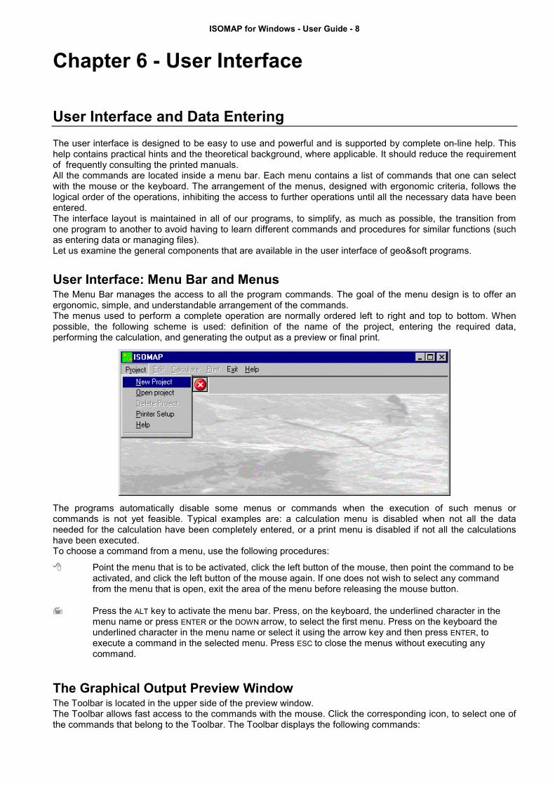
User Interface: Menu Bar and MenusThe Menu Bar manages the access to all the program commands. The goal of the menu design is to offer anergonomic, simple, and understandable arrangement of the commands.The menus used to perform a complete operation are normally ordered left to right and top to bottom. Whenpossible, the following scheme is used: definition of the name of the project, entering the required data,performing the calculation, and generating the output as a preview or final print.

The programs automatically disable some menus or commands when the execution of such menus orcommands is not yet feasible. Typical examples are: a calculation menu is disabled when not all the dataneeded for the calculation have been completely entered, or a print menu is disabled if not all the calculationshave been executed.To choose a command from a menu, use the following procedures:

Point the menu that is to be activated, click the left button of the mouse, then point the command to beactivated, and click the left button of the mouse again. If one does not wish to select any commandfrom the menu that is open, exit the area of the menu before releasing the mouse button.

Press the ALT key to activate the menu bar. Press, on the keyboard, the underlined character in themenu name or press ENTER or the DOWN arrow, to select the first menu. Press on the keyboard theunderlined character in the menu name or select it using the arrow key and then press ENTER, toexecute a command in the selected menu. Press ESC to close the menus without executing anycommand.

The Graphical Output Preview WindowThe Toolbar is located in the upper side of the preview window.The Toolbar allows fast access to the commands with the mouse. Click the corresponding icon, to select one ofthe commands that belong to the Toolbar. The Toolbar displays the following commands:


- Zoom + : clicking the first icon activates the ZOOM function (it can only be used with the mouse) thatpermits the enlargement of part of the drawing. The function remains active until the Zoom - icon is selected.To enlarge a part of the drawing:

click the icon, and then select the area to be enlarged by clicking the upper-left corner and draggingthe mouse pointer to the lower-right corner. At this point, release the mouse button. Note: due to thelow resolution of the screen, the texts could appear in a slightly different scale at different zoom levels.This does not affect the quality of the final printouts.

- Zoom - : click this icon to return to the original scale of the preview.

- Arrows: click the arrow icons, in "Zoom + " mode, to pan the on-screen preview.

- Print: click the print icon to send the drawing to the default printer.

- Resized print: click this icon to send the drawing to the default printer. The image will be resized to fit thecurrent paper size.

- DXF: one can export the graphic output as a DXF file by clicking this icon; it gives access to a dialoguewindow that enables one to assign a different name to the DXF file, which has, by default, the same nameas the current project.

- EMF/W: This icon allows the graphic output to be exported to a version of the Enhanced Windows Metafilewhich is compatible with Microsoft Word. Clicking this icon gives access to a dialogue window that enablesone to assign a different name to the EMF file, which has, by default, the same name as the current project.

- EMF/D: This icon allows the graphic output to be exported to a version of the Enhanced Windows Metafilewhich is compatible with Corel Draw. Clicking this icon gives access to a dialogue window that enables oneto assign a different name to the EMF file, which has, by default, the same name as the current project.

- Exit: click this icon to close the preview window and return to the main menu.

The Input Dialogue WindowsThe different menu commands can perform an immediate action, or display a dialogue window in order to inputor edit the various data sets.When a dialogue window is visible, all the actions that do not pertain to it are ignored. Hence, it is necessary toclose the dialogue window to resume the normal use of the program.

Some fundamental tools are used inside the dialogue windows: data fields such as text and list boxes, andbuttons.


The text boxes are used to input numerical values and text strings. Most of the editing keys (HOME, END, INS,DEL, etc.) can be used inside these fields. If one sees a small arrow pointing down on the right side of the datafield, one has a list box.To scroll the list box and select an item, do as follows:

click the arrow, and then click the item to be selected.

press the DOWN arrow until one arrives at the item to be selected. It is also possible to press a letter todirectly reach the first item that begins with that letter.

Tere are three buttons in the dialogue window:

• <Ok> - this button saves the entered information and goes on to the next phase.

• <Cancel> - this button closes the Dialogue window without saving the just entered data, or withoutexecuting the command.

• <Help> - this opens a window that contains general information on how to use the dialogue windows.

To use the buttons:

click the button

press alt+underlined letter

To edit the data inside the dialogue window, use the following keys:

• TAB - moves the cursor to the next field; when the cursor is inside the last visible field the cursor goes to thefirst control button of the Dialogue window. To return to the previous field, press SHIFT+TAB.

• ENTER - moves the cursor to the next field. If the cursor is positioned on one of the window buttons, thecorresponding command is executed.

• BACKSPACE - cancels the last character that has been entered.

• DEL - cancels the character to the right of the cursor.

• ESC - closes the Dialogue window without saving the entered values or without executing the command. The<Cancel> button will do the same.

• UP ARROW/ DOWN ARROW - these are used in multiple fields, or those fields that have a list box.

• LEFT ARROW/ RIGHT ARROW - moves the cursor to the previous or next field.

• HOME -moves the cursor to the beginning of the field.

• END - moves the cursor to the end of the field.

A yellow box with a short text that explains the meaning of the value to be entered, can be seen in the lower partof the window. If the text is not completely visible, click the yellow box to read the complete text.

Data Input With TablesTables are used to enter long sequences of numerical values and/or text strings. The keys to be used are thefollowing:

• TAB - moves the cursor to the first button in the window. When one presses this key again, the cursor ismoved to the next button.

• SHIFT+TAB - moves the cursor to the previous button.

• ENTER - moves the cursor into the next input field. If the cursor is positioned on one of the window buttons,the corresponding command is executed.

• PAGE UP - moves the cursor up 15 lines.

• PAGE DOWN - moves the cursor forward 15 lines.

• UP ARROW - moves the cursor to the input field directly above.

• DOWN ARROW - moves the cursor to the input field directly below.

• LEFT ARROW / RIGHT ARROW - moves the cursor to the field respectively to the left or to the right of the currentposition.

• HOME - moves the cursor to the beginning of the line.


• END - moves the cursor to the end of the line.

• F2 - copies the field contents to the extended editing field under the title bar in order to facilitate the editingof the long strings. When working in this editing field, please REMEMBER to press ENTER, even beforeclicking the <Ok> button. Double-clicking a field has the same effect as pressing the F2 key.

The tables have two additional buttons:

• <Insert> - creates an empty line before the one in which the cursor is positioned.

• <Delete> - deletes the line in which the cursor is positioned.

IMPORTANT SUGGESTION: you can copy data to or from other programs such as Microsoft Excel:

The data entered in the table can be copied in order to be pasted into another table.To copy the table’s contents:

press the key combination CTRL+C. The contents will be copied into the Clipboard of Windows.

To paste the Clipboard contents into the table:

press the key combination SHIFT+INS, or CTRL+V.

A yellow box with a short text that explains the meaning of the value to be entered, can be seen in the lower partof the window. If the text is not completely visible, click the yellow box to read the complete text.

Message WindowsThe function of these windows is to give information to the user concerning the system status, as in the case ofan error due to an improper use of the program.


Help On LineA complete Help On Line is available. It is possible to ask for information or suggestions related to thecommands or the use of the program. In order to access the help on line, proceed as follows:

1. Position the cursor on a field of a dialogue window and press F1.

2. Use the Summary from the Help menu.


Chapter 7 - Introduction to the ISOMAP module

Introduction to the ISOMAP moduleISOMAP is the module that is used to calculate and render surfaces through contour lines or coloured andshaded areas with a high degree of precision. The program allows the representation of the surface both intopographic map and perspective view forms.The calculation is performed in two stages. The first stage consists of creating a regular grid from a collection ofarbitrarily positioned points. The second stage consists of drawing the surface using the previously created grid.The first stage can be performed using three methods: the inverse distance method, the kriging method, and anew interpolation and extrapolation method based on a weighted average of polynomial surfaces.The use of this polynomial algorithm makes it possible to generate points that are external to the area of thesampled locations in such a way as to maintain the trend of the surface, even when this surface cannot beapproximated by a simple horizontal plane.This feature is especially useful for those problems that deal with the surface gradient, such as flow line tracingor rockfall analysis. The commonly used extrapolation algorithms based on the weighted average (includingkriging) can lead to large errors, for example to the inversion of the flow direction in the peripheral areas of themap.The use of a polynomial algorithm to create a grid also yields a more realistic surface of the area where thesampled locations can be found, as the evaluation is less sensitive to the spatial distribution and point density.The regular square grid is then interpolated with bi-cubic splines to obtain a continuous surface that iscontinuously differentiable and which passes through the grid nodes.

The ISOMAP module has the following basic operations:

• Grid Generation

• Slope Map

• Exposure Map

• Grid Difference

• Linear Transformation

• Filtering

• Grid Duplication

• DTM Import

These operations are described later in this chapter.

Grid Generation (ISOMAP module)The basis of any project is the generation of a regular grid. The square grid is generated using one of theavailable methods, starting from a set of arbitrarily positioned points sampled on the surface under examination.The more regular the disposition and density of the input points are, the more reliable the final result will be,regardless of which calculation method is used. Let us consider the calculation methods that can be used.

Weighted AverageThe value for unsampled locations is equal to the weighted average of the values of the nearby samples. Theweighted average takes the following form:

Z'(p) = /(Z(i) * (1 / D(i, p) )) (1 / D(i, p) )i=1

n

i=1

nα α∑ ∑

where:Z'(p) = estimated value at point pZ(i) = sampled value at point iD(i,p) = distance between point p and point i


alpha = weighting exponentn = number of sampled points

This kind of interpolation is unbiased if the sum of the weights equals one. This is true for the inverse-distanceweighted method because the sum of the weights divided by the sum of the weights is equal to one.The exponent on the distance function above can be altered. Altering the exponent on the distance affects therelative weights of the points. In all cases, a sample that is further from the point to be estimated will receive alower weight.As the exponent is increased, the relative influence of more distant points decreases.A problem that exists with this method is that you have to make a guess at what the exponent should be, andthere is no assurance that your guess is correct.

Kriging

The Kriging algorithm, also called “best linear unbiased estimator”, was developed for mining geology. It is“best” because it minimizes the error variance in the estimate, “unbiased” because the weights sum to one, and“linear” because it is a simple weighted average. It also uses a weighted average method to calculate the valueat unsampled locations, but rather than guessing at the relationship between similarity of values and distance(like we do when we guess at the exponent in inverse-distance methods), the relationship is calculated from thedata using the semivariogram.Once the lognormal semivariogram has been calculated, the weights L(i) can be obtained to estimate the valueof an unsampled location. The Kriging takes the following form:

Z'(p) = (Z(i) * L(i))i=1

n

∑

where:Z'(p) = estimated value at point pZ(i) = sampled value at point in = number of sampled pointsThis set of weights has the property L(i) = 1∑and guarantee the minimisation of the general expression that represents the variance of the error associated tothe estimate relative to point p.

2 * ( L(i) * G(D(i, p)) - g( D(p, p))

i = 1

n- ( ( L(i) * L( j) * G(D(i, j))))

j = 1

n

i = 1

n ∑ ∑∑

2 * ( L(i) * G(D(i, p)) - g( D(p, p))

i = 1

n- ( ( L(i) * L( j) * G(D(i, j))))

j = 1

n

i = 1

n ∑ ∑∑

where:G(D(x,y)) = average variance associated to the distance between the points x and yn = number of sampled pointsThis minimisation is obtained through the solution of a system of n+1 linear equations.

Method of the Weighted Average of Polynomial SurfacesOne of the greatest problems of the previously described methods is the impossibility of estimating valuesoutside the range defined by the maximum and minimum values of the sampled points. This problem has theimmediate consequence of preventing one from extrapolating, in a significant way, the values beyond the areathat is actually covered by the sampled points.Hydrogeology or rockfall analysis applications, based on the treatment of partial derivatives of the surface(gradients), are in fact extremely sensitive to irregularities, even small ones, of the surface.For this reason a more complex algorithm has been made available, that is based on an auxiliary polynomialestimator Z"(i) which represents the regional trend of the variable under examination.The estimate therefore assumes the following form:

Z'(p) = / (Z" (i) * (1 / D(i, p) )) (1 / D(i, p) )i=1

n

i=1

nα α∑ ∑

where:Z'(p) = estimated value at point p


Z"(i) = estimated value in function of the value assumed at point iD(i,p) = distance between point p and point ialpha = weight exponentn = number of sampled points

Procedure- Select the “New Project” command from the “Project” menu- Choose a new name for the project- Select “Grid Generation” in the “Operation” window- Use the “Edit Points” in the “Edit” menu to input the spot sampled points- Use the “Grid Parameters” in the “Edit” menu to choose how the grid will be calculated- Select “Calculation” on the menu bar

Slope Map (ISOMAP module)With this command, the program creates a grid that contains the slope (in degrees) of a topographic surface.It is possible to choose whether the program has to calculate the maximum or the average slope of the groundaround each node of the grid. As ji , are the grid node indexes and l is the mesh size, we obtain:

maximum slope =

2222 /)),()1,(),,()1,(max(/)),(),1(),,(),1(max( ljizjizjizjizljizjizjizjiz −−−++−−−+

average slope =2222 4/))1,()1,((4/)),1(),1(( ljizjizljizjiz −−++−−+

Procedure- Select the “New Project” command from the “Project” menu- Choose a new name for the project- Select “Maximum Slope Map” or “Average Slope Map” in the “Operation” window- Select the project that contains the original topographic surface- Select “Calculation” on the menu bar

Exposure Map (ISOMAP module)With this command, the program creates a grid that contains the angle from the North of the dip direction of theground. The Y-axis must be oriented to the North. The South direction will result to be equal to 180°; both theEast and West directions will be equal to 90°.

Procedure- Select the “New Project” command from the “Project” menu- Choose a new name for the project- Select “Exposure Map” in the “Operation” window- Select the project that contains the original topographic surface- Select “Calculation” on the menu bar

Note: as an alternative, it is possible to obtain interesting results working on the original topographic surfaceusing a horizontal Light Vector.

Grid Difference (ISOMAP module)With this command, the program creates a new grid that is calculated as the node-by-node subtraction of twogiven grids. A typical application could be the evaluation of the removed ground, which is obtained bysubtracting two grids that represent the topographic surface before and after an excavation.It is mandatory that the two grids have the same number of rows and columns.

Procedure- Select the “New Project” command from the “Project” menu- Choose a new name for the project- Select “Grid Difference” in the “Operation” window- Select the project to extract from the “minuend” grid


- Select the “Select Subtrahend Grid” command from the “Edit” menu- Choose an existing project (of the same grid size) to extract from the “subtrahend” grid- Select “Calculation” on the menu bar

Linear Transformation (ISOMAP module)The linear transformation operator makes it possible to perform a linear transformation of the surface,performing the following three sequential operations for each node:

1. sums a first translation factor (a);2. multiplicates by a scale factor (b);3. sums a second translation factor (c).

The general formula z'=(z+a)*b+c makes it possible to perform any linear transformation such as the Celsius-Fahrenheit conversion, with a=0, b=9/5 and c=32.

Procedure- Select the “New Project” command from the “Project” menu- Choose a new name for the project- Select “Linear Transformation” in the “Operation” window- Select the project to be transformed- Select the “Linear Transformation Parameters” command from the “Edit” menu- Select “Calculation” on the menu bar

Filtering (ISOMAP module)This operator performs a numerical filtering in the space domain, that is to say, the convolution of a matrixoperator of order 2n+1 with the grid itself.The filters should always be symmetrical to the axis that passes through its centre, and to the two diagonals.By using a unit matrix one will obtain a grid that is the moving average of the original grid. By using thiscommand in conjunction with the Grid Difference operation, one can, for example, separate the local gravityanomalies from the regional ones.

Procedure- Select the “New Project” command from the “Project” menu- Choose a new name for the project- Select “Filtering” in the “Operation” window- Select the project to be filtered- Select the “Select Filter” command from the “Edit” menu- Choose a filter (you can create a new one with a text editor)- Select “Calculation” on the menu bar

Grid Duplication (ISOMAP module)This command enables one to duplicate a project, for example to allow parametric analyses.It can also be used to create a new grid from an existing one, changing the extension of the grid and the size ofthe mesh.

Procedure- Select the “New Project” command from the “Project” menu- Choose a new name for the project- Select “Grid Duplication” in the “Operation” window- Select the project to be duplicated- Assign the new values of Xmin, Xmax, Ymin, Ymax and of the Mesh Size- Select “Calculation” on the menu bar

Note: the X,Y values must be inside the ranges of the original grid.

DTM Import (ISOMAP module)With this command, it is possible to import regular grid data from other programs and convert these into theISOMAP format. A default ISOMAP format can be used, or a custom made filter can be developed on request.


The data files must previously have been created, with a text editor such as Notepad, and have the “.ZRE”extension.The structure of the ZRE files is quite simple: on the first line write the number of nodes on the X-axis, on thesecond line write the number of nodes on the Y-axis, on the third line write the mesh size (in metres) betweentwo nodes, in the two next lines write the abscissa and ordinate of the first grid node in the bottom left corner.The file can now be completed with the Z-values, column by column (left to right), each column in a bottom-uporder. Each column of Z-values must be preceded by a line that contains the text “Column #”, where # is thecolumn number. Once the file is saved, the import procedure can be started.

Procedure- Select the “New Project” command from the “Project” menu- Choose a new name for the project- Select “Import ZRE file” in the “Operation” window- Choose the ZRE file you want to import the grid from


Chapter 8 - ISOMAP family - GeneralCommands

Project Menu (ALT,R)This menu contains all the commands that are used to open and delete the files which contain all the projectdata. As long as the project name has not been defined, the other menu items are disabled.

The last opened projects are shown in the lower part of this menu.

New Project Command (ALT,R,N)In order to operate with this program, it is necessary to open a project; this can be a new project or an alreadyexisting one. To open a new file:

choose the New Project command from the menu by first clicking the Project menu item and then onthe New Project command. Type the name of the new file in the File Name field and confirm.

choose the New Project command from the menu by using the combination of the keys ALT,R,N. Typethe name of the new file in the File Name field and press ENTER.

The name of the file in use will be reported in the title bar of the main window.The name of the file should not contain spaces and/or punctuation marks. It is not necessary to indicate anyextension, since the extension “.NFJ” is automatically added: for example, given the name “TEST01”, the filename “TEST01.NFJ" will be internally used by the program.When opening a new project, it is necessary to choose which operation has to be performed. Only oneoperation can be associated to each project name, and it cannot be changed later on.It is possible to create a series of projects, each of which uses the results of a previously elaborated project as a“starting point”: this will be the Source Project.


See "Introduction to the ISOMAP module" for information about the Grid Generation, Slope Map, Exposure Map,Grid Difference, Linear Transformation, Filtering, Grid Duplication and DTM Import operations.

There is no specific command In the program to save data, as these are automatically saved after each dataentry or elaboration.

Open Project Command (ALT,R,O)In order to operate with this program, it is necessary to open a project; this can be a new project or an alreadyexisting one. To open an existing file:

choose the Open Project command from the menu by first clicking the Project menu item and then onthe Open Project command from the menu. Type or double click the name of the new file in the FileName field and confirm.

choose the Open Project command from the menu by using the combination of the keys ALT,R,O. Typethe name of the file in the File Name field then press ENTER. Otherwise press TAB and then the UPARROW or DOWN ARROW to select the name from the list, then press ENTER.

The name of the file in use will be reported in the title bar of the main window.There is no specific command In the program to save data, as these are automatically saved after each dataentry or elaboration.


Delete Project Command (ALT,R,D)This makes it possible to delete all the files pertaining to a project. Before using this command, one should besure that these data are no longer necessary. Particular care must be taken if the project has been used as aSource Project for other elaborations. Before deleting the files, the program asks for confirmation.

Printer Setup Command (ALT,R,P)When selecting this command, one calls the printer configuration dialogue window. Here one can verify andmodify the default printer setup or select another printer from the list of the installed ones.

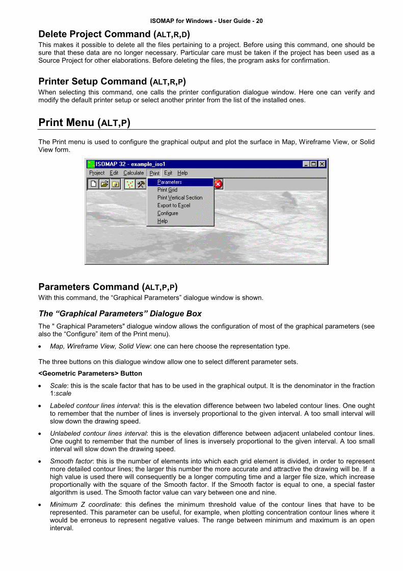
Print Menu (ALT,P)The Print menu is used to configure the graphical output and plot the surface in Map, Wireframe View, or SolidView form.

Parameters Command (ALT,P,P)With this command, the “Graphical Parameters” dialogue window is shown.

The “Graphical Parameters” Dialogue BoxThe " Graphical Parameters" dialogue window allows the configuration of most of the graphical parameters (seealso the “Configure” item of the Print menu).

• Map, Wireframe View, Solid View: one can here choose the representation type.

The three buttons on this dialogue window allow one to select different parameter sets.

<Geometric Parameters> Button

• Scale: this is the scale factor that has to be used in the graphical output. It is the denominator in the fraction1:scale

• Labeled contour lines interval: this is the elevation difference between two labeled contour lines. One oughtto remember that the number of lines is inversely proportional to the given interval. A too small interval willslow down the drawing speed.

• Unlabeled contour lines interval: this is the elevation difference between adjacent unlabeled contour lines.One ought to remember that the number of lines is inversely proportional to the given interval. A too smallinterval will slow down the drawing speed.

• Smooth factor: this is the number of elements into which each grid element is divided, in order to representmore detailed contour lines; the larger this number the more accurate and attractive the drawing will be. If ahigh value is used there will consequently be a longer computing time and a larger file size, which increaseproportionally with the square of the Smooth factor. If the Smooth factor is equal to one, a special fasteralgorithm is used. The Smooth factor value can vary between one and nine.

• Minimum Z coordinate: this defines the minimum threshold value of the contour lines that have to berepresented. This parameter can be useful, for example, when plotting concentration contour lines where itwould be erroneus to represent negative values. The range between minimum and maximum is an openinterval.


• Maximum Z coordinate this defines the maximum threshold value of the contour lines that have to berepresented. This parameter can be useful when one wants to eliminate values that are too high, such asthe borders of polynomial extrapolations.

• Zero range to hide: this parameter allows one to hide the contour lines close to zero. This option is useful,for example, for the representation of magnetometric data.

• Vertical exaggeration factor: this factor enables one to stress the drawing, thus enhancing the anomalies ofthe plotted quantity.

• Viewpoint distance: this is only used in the Solid View. It is the absolute distance (in meters) between theviewpoint and the centre of the grid. This parameter is not used in the Wireframe View, because, in thiscase, the viewpoint distance is considered to be infinite.

• Viewpoint Vector X , Y, Z components: these define the direction of the viewpoint from the centre of the grid.The program disregards the vector magnitude, and automatically considers only the direction. It is used bothin the Solid View and in the Wireframe View.

• Light Vector X , Y, Z components: these define the direction of the light point from the centre of the grid. Ifthe three coordinates are equal to zero, no light effect is added. These parameters are used in the Map andin the Solid View.

• Sampled locations: one can decide if and how the sampled locations will be drawn. The available optionsare: a simple cross, a cross labeled with the value of the sample, a cross labeled with the name of thelocation, or no representation at all.

<Vectors and Titles> Button

• Flow vectors: with this option it is possible to draw flow vectors as small arrows positioned on the gridnodes. There are three options: Direction - unit vectors are drawn, oriented towards the dip direction;Velocity - the velocity vectors are drawn, as defined in Darcy’s law, with the lengths proportional to theproduct of the hydraulic head gradient and the hydraulic conductivity; Gradient - flow vectors are shown asarrows oriented towards the dip direction: the vector length is proportional to the dip of the surface. Novector is drawn with the No Vector option.

• Vector step: this is used to space the vectors further apart; when assigning a value equal to 3, a vector, forexample, will be drawn every three grid nodes.

• Vector length / mesh width ratio: the maximum (or unit) length of the vectors is, by default, equal to themesh width. It is possible to to alter this value by assigning a vector length / mesh width ratio that is differentfrom one.

• Lines: this is used to draw a set of continuous flow lines. The required data are: the X,Y coordinates of the


end points of an imaginary segment, and the number of equally spaced points along this segment throughwhich the flow lines will pass.

• Titles: entering a title or sub-titles is not mandatory.

• Legend Caption: when a Map or a Solid View is coloured, a legend is automatically added. It is possible toadd a caption to describe the plotted quantity.

• Legend check box: unchecking this box, the legend will not be plotted; this option is useful to export a“clean” graphic output to other programs like GIS.

<Colour Selection> Button

• Number of colours lower than: the program automatically detects the optimal contour line intervals, usingmultiples of 1.0En, 2.0En and 5.0En. Setting the Number of colours lower than parameter, the program isforced to choose a value of the contour line interval that produces a number of contour lines (and colourranges) lower than the given value.

• “Reset intervals” button: this button activates a procedure that recalculates the contour line intervals as afunction of the previous parameter.

• Scale type: the colour shade distribution can be organised using different scale types: linear, inverse linear,logarithmic, inverse logarithmic, quadratic or inverse quadratic.

• Colour type: the colour sets can be generated in different ways: Black and White, Red, Green, Blue,Multicolour, and Random. With the Black and White option one obtains a grey-scale output; With the Red,Green or Blue option the selected colour shades towards white; the Multicolour options allows one to createoutputs using a continuous scale of colours, and the Random option assigns a colour that is randomlychosen to each level.

• Disable surface colouring: when this option is activated, the program does not colour the areas between thecontour lines.

• R/G/B shade to black: with this option the selected colour will shade towards black instead of towards white.

• Disable contour lines: when this option is activated, the program no longer draws the contour lines; if bothsurface colouring and contour lines are disabled, nothing appears on the graphical output.

• Remove violet from multicolour: this option allows one to start the multicolour scale (if selected) from theblue instead of from the violet colour.

• Use manual colour settings: one can choose to manually define the contour line values and the colours to fillthe area between the adjacent contour lines. To manually define those parameters, click the <ManualColour Setting> button.

• The <Copy Colour Set> Button: If the current interval number is lower than 21, the "Manual Colour Setting"


dialogue box is opened, and the current settings are copied and can then be modified, otherwise the buttonis disabled.

The <Manual Colour Setting> ButtonThe <Manual Colour Setting> button opens the "Manual Colour Setting" dialogue box, where you can define thecontour line values and the colour one wishes to assign to each interval. These settings can be saved aspersonalised colour profiles.To change a colour, double click the coloured field and choose the new colour to be assigned to the intervalfrom the Colours Dialogue Box.Each time a colour set has been defined and confirmed, it is saved as a default manual colour profile. It will thenbe used each time the Use manual colour settings option is selected, if a different colour profile has not beenloaded or saved; in this case, the default colour profile is overwritten, and the selected (saved or loaded) colourprofile will be permanently associated to the current project, regardless of the default manual colourconfiguration.


• <New Profile> button: if the current interval number is lower than 21, the current automatic settings arecopied and can then be modified, otherwise all the fields are cleared.

• <Read Profile> button: the program reads a previously saved colour profile from the hard disk; this colourprofile will be permanently associated to the current project.

• <Save Profile> button: this allows one to save the current colour profile on the hard disk; this colour profilewill be permanently associated to the current project.

Print Grid Command (ALT,P,G)With this command, the Print Preview window is opened and the plot is shown; it is then possible to directly printthe graphical output, or export it to different formats.More: The Graphical Output Preview Window

Print Vertical Section Command (ALT,P,V)With this command, a window is shown that allows the graphic output of a ground vertical section to beconfigured.

The “Vertical Section Configuration” Dialogue boxA certain number of points along a given line are calculated and plotted as a vertical section. The requiredparameters are:

• Point Distance: distance between two adjacent calculated points along the given line [m].

• Reference Elevation: elevation of the reference plane [m].

• Horizontal Scale: horizontal scale of the graphical output.

• Vertical Scale: vertical scale of the graphical output. The scales are separated to allow a verticalexaggeration factor.

• Abscissa, Ordinate: the X and Y planimetric coordinates of the nodes of the line, from the arbitrary originused to create the grid, along which the calculated points are aligned.

• Ok Button: the print preview window is shown, and the vertical section is plotted.

• Cancel Button: this is used to abort the current operation.

Export to Excel Command (ALT,P,X)With this command, a window is shown to allow one to select which quantity has to be exported as an SLK file(a format that is compatible with Microsoft Excel and other spreadsheets).


Configure Command (ALT,P,C)With this command, one can define the graphical properties of the different objects in the graphical output.

One can associate a colour, a line thickness and a character font to each object. Notice that not all the objectshave both a line thickness and a character font: for example, a title only requires the colour and the characterfont to be defined.

• Click an object to select it (use the scroll bar to see the entire list)

• Click one of the option buttons, in the “colours” frame, to select the colour that has to be associated to theselected object. The Not drawn option hides the object of the graphical output.

• If the object contains texts, one can choose a character font from the list (use the scroll bar to see the entirelist)

• If the object contains lines, one can assign a thickness to the lines (in mm). If the value is zero, the programuses the thinnest line on the output device.

• It is possible, as an option, to assign a left and a top margin (in cm) to the whole graphical output.

NOTE: although the available set is limited to fifteen colours, they can be manually customised; double-click thecoloured bar to open the Colour Dialogue Box and choose a different RGB value associated to the selectedcolour.

Exit Menu (ALT,X)This command allows one to exit the program. There is no specific command to save the entered data as theseare automatically saved each time they are modified.


Chapter 9 - ISOMAP Menus - Grid Generation

Edit Menu (ALT,E) - Grid GenerationThis menu is used to enter and edit the input data used in the gridding operations.

Data Points Command (ALT,E,P)This enables one to enter and edit the input data points.

The “Data Points” Dialogue boxThe following data should be entered in the “Data Points” window:

• X and Y Coordinates: the planimetric coordinates should be entered (in metres) from an arbitrary origin.

• Elevation: the ground elevation (or another physical quantity) that has to be represented on the Z-axis.

• Name: this is an optional caption of the data points. There are two special characters that can be added atthe beginning of the point names (notice that those characters will not be printed on the graphical output):when the point name begins with the @ character, the value will be used in the calculation but will not beprinted; when the point name begins with the # character, the data point will be printed (if one of the


Sampled locations options has been selected) but will not be used in the calculation.

Gridding Parameters Command (ALT,E,G)The Isomap module creates a regular grid that calculates the values of the physical quantity for each node of asquare mesh using different interpolation algorithms. The required parameters are entered in the GriddingParameters dialogue box.

The “Gridding Parameters” Dialogue BoxThe following data are entered in the “Gridding Parameters”:

• Calculation Algorithm: the calculation of the grid can be performed using the Kriging or the WeightedAverage of Polynomial Surfaces; a zero-order polynomial surface is a special case that corresponds to theordinary inverse-distance weighted average method.

• Order of the polynomial surface: the basic concept of the Weighted Average of Polynomial Surfaces is thatthe best fitting polynomial surface is calculated, as a first step, from the data points, then a gradual verticalshift allows one to obtain a final surface that passes through the sampled locations. Going away from thesampled points, the calculated surface converges to the best fitting polynomial surface. A zero-orderpolynomial surface (Z = a) is a special case that corresponds to the classic inverse-distance weightedaverage method. A fist-order polynomial surface (Z = a + b X + c Y) is a dipping plane that gives, forexample, a good approximation for a simple water table only sampled in three wells. The surfaces of thesecond and third order are more complex and can better approximate a surface with many sampledlocations. These surfaces require a homogeneous distribution of the sampled points because the gradient ofthe surface rapidly increases as it becomes distant from the sampled area.

• Mesh size: the mesh size (in metres) should be such as not to exceed 500 grid elements along each X andY axe; if this value is exceeded, the mesh size is automatically adjusted.

• Threshold distance: this is the radius (in metres) of the circle wherein the points that will be considered tocalculate a single grid value lie. As the used methods are based on an inverse-distance weighted average, itcould be a good idea to keep this value sufficiently large so as to consider all the sampled points in thecalculations, thus also obtaining a smoother surface with a small mesh size.

• Weighting exponent: this is the exponent that is applied to the inverse distance which is used in theweighted averages. The greater the exponent, the greater is the influence of a sampled point on thecalculated grid. This means that too small exponent values can generate a surface with “peaks” aroundeach sampled point, while too large exponent values can generate a “benched” surface. Values between 4and 6 can normally yield good results.

• Minimum X coordinate: together with the ordinate of the lower side, this defines the lower left corner of thegrid.

• Maximum X coordinate: together with the ordinate of the upper side, this defines the upper right corner of


the grid.

• Minimum Y coordinate: together with the abscissa of the left side, this defines the lower left corner of thegrid.

• Maximum Y coordinate: together with the abscissa of the right side, this defines the upper right corner of thegrid

ExampleExample: an original surface, with data points regularly sampled on each grid node, has been made denser toshow the effect of the Weighting exponent. The best result has been obtained with Exponent = 3.

Original surface Exponent = 3Exponent values 1 and 2 produced a surface with “peaks” around each sampled point (particularly emphasisedwith the minimum value); on the other hand, Exponent values 4 and 8 produced a “benched” surface(particularly emphasised with the maximum value).

Exponent = 1 Exponent = 2 Exponent = 4 Exponent = 8

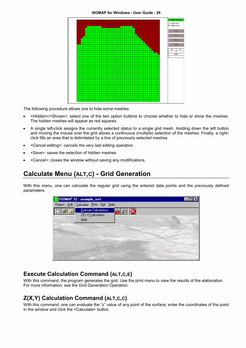
Hidden Mesh Selection Command (ALT,E,M)This command allows one to hide some of the grid meshes. A graphical editing window is opened and the grid isshown: by default, all the meshes are not hidden, and appear as green squares.


The following procedure allows one to hide some meshes:

• <Hidden>/<Shown>: select one of the two option buttons to choose whether to hide or show the meshes.The hidden meshes will appear as red squares.

• A single left-click assigns the currently selected status to a single grid mesh. Holding down the left buttonand moving the mouse over the grid allows a continuous (multiple) selection of the meshes. Finally, a right-click fills an area that is delimitated by a line of previously selected meshes.

• <Cancel editing>: cancels the very last editing operation.

• <Save>: saves the selection of hidden meshes.

• <Cancel>: closes the window without saving any modifications.

Calculate Menu (ALT,C) - Grid GenerationWith this menu, one can calculate the regular grid using the entered data points and the previously definedparameters.

Execute Calculation Command (ALT,C,E)With this command, the program generates the grid. Use the print menu to view the results of the elaboration.For more information, see the Grid Generation Operation.

Z(X,Y) Calculation Command (ALT,C,C)With this command, one can evaluate the “z” value of any point of the surface; enter the coordinates of the pointin the window and click the <Calculate> button.


The program calculates the required value using a bi-cubic splines interpolation algorithm, and displays theresult in the "Z" field.

Print Menu (ALT,P)The Print menu is used to configure the graphical output and to plot the surface in Map, Wireframe View or SolidView form.For more information, see the Print Menu - Common Commands.


Chapter 10 - ISOMAP Menus - Slope Map

Edit menu (ALT,E) - Slope MapWith this command, the program creates a grid that contains the slope (in degrees) of a topographic surface.When creating the new project, it is possible to choose whether the program has to calculate the maximum orthe average slope of the ground around each node of the grid.

Hidden Mesh Selection Command (ALT,E,M)This command allows one to hide some of the grid meshes.For more information, see the Hidden Mesh Selection in the ISOMAP Menus - Grid Generation.

Calculate Menu (ALT,C) - Slope MapThis menu allows one to calculate a grid that contains the slope of a topographic surface (in degrees).For more information, see the Slope Map Operation.

Execute Calculations Command (ALT,C,E)This command allows one to calculate the slope of a topographic surface (in degrees).Use the print menu to view the results of the elaboration.

Z(X,Y) Calculation Command (ALT,C,C)With this command, one can evaluate the “z” value of any point of the surface.For more information, see the Z(X,Y) Calculation in the ISOMAP Menus - Grid Generation.

Print Menu (ALT,P) - Slope MapThe Print menu is used to configure the graphical output and to plot the surface in Map, Wireframe View or SolidView form.For more information, see the Print Menu - Common Commands.


Chapter 11 - ISOMAP Menus - Exposure Map

Edit menu (ALT,E) - Exposure MapWith this command, the program creates a grid that contains the angle from the North of the dip direction of theground. The Y-axis must be oriented to the North. The South direction will result to be equal to 180°; both Eastand West directions will be equal to 90°.


Calculate Menu (ALT,C) - Exposure MapThis menu allows one to calculate the angle from the North of the ground dip direction.For more information, see the Exposure Map Operation

Execute Calculations Command (ALT,C,E)This command allows one to calculate the angle from the North of the ground dip direction.


Print Menu (ALT,P) - Exposure MapThe Print menu is used to configure the graphical output and plot the surface in Map, Wireframe View, or SolidView form.For more information, see the Print Menu - Common Commands.


Chapter 12 - ISOMAP Menus - Grid Difference

Edit menu (ALT,E) - Grid DifferenceWith this command, the program creates a new grid that is calculated as the node-by-node subtraction of twogiven grids. A typical application could be the evaluation of the removed ground, which is obtained bysubtracting two grids that represent the topographic surface before and after an excavation.It is mandatory that the two grids have the same number of rows and columns.


Select Subtrahend Grid Command (ALT,E,G)This command allows one to choose an existing project (of the same grid size) to extract from the “subtrahend”grid

The “Select Subtrahend Grid” Dialogue BoxTo select a file, type the name of the project to extract from the “subtrahend” grid in the File Name field, orbrowse the hard disk and double-click the project file name.

Calculate Menu (ALT,C) - Grid DifferenceOnce selected the Subtrahend Grid, this menu allows one to calculate the grid difference as the node-by-nodesubtraction of the two given grids.

Execute Calculations Command (ALT,C,E)Once selected the Subtrahend Grid, this command calculated the grid difference as the node-by-nodesubtraction of the two given grids. Use the print menu to view the results of the elaboration.For more information, see the Grid Difference Operation.



Print Menu (ALT,P) - Grid DifferenceThe Print menu is used to configure the graphical output and plot the surface in Map, Wireframe View, or SolidView form.For more information, see the Print Menu - Common Commands.


Chapter 13 - ISOMAP Menus - LinearTransformation

Edit Menu (ALT,E) - Linear TransformationsThe linear transformation operator makes it possible to perform a linear transformation of the surface,performing the following three sequential operations for each node:

1. sums a first translation factor (a);2. multiplicates by a scale factor (b);3. sums a second translation factor (c).

The general formula z'=(z+a)*b+c makes it possible to perform any linear transformation such as the Celsius-Fahrenheit conversion, with a=0, b=9/5 and c=32.


Linear Transformation Parameters Command (ALT,E,T)This command enables one to define the parameters for the linear transformation.

The “Linear Transformation Parameters” Dialogue boxIn the “Linear Transformation Parameters” dialogue window the following data are required:

• First translation factor: it is the constant a in the linear transformation z'=(z+a)*b+c formula.


• Scale factor: it is the scale factor ‘b’ in the linear transformation formula.

• Second translation factor: it is the constant 'c' in the linear transformation formula.

Calculate Menu (ALT,C) - Linear TransformationWith this menu, a linear transformation is performed on each node of the source grid.

Execute Calculations Command (ALT,C,E)With this command, the linear transformation is performed on each node of the source grid, using the givenparameters.For more information, see the Linear Transformation Operation.


Print Menu (ALT,P) - Linear TransformationThe Print menu is used to configure the graphical output and plot the surface in Map, Wireframe View, or SolidView form.For more information, see the Print Menu - Common Commands.


Chapter 14 - ISOMAP Menus - Filtering

Edit Menu (ALT,E) - FilteringThis operator performs a numerical filtering in the space domain, that is to say, the convolution of a matrixoperator of order 2n+1 with the grid itself.The filters should always be symmetrical to the axis that passes through its centre, and to the two diagonals.By using a unit matrix one will obtain a grid that is the moving average of the original grid. By using thiscommand in conjunction with the Grid Difference operation, one can, for example, separate the local gravityanomalies from the regional ones.


Select Filter Command (ALT,E,F)With this command, the program shows the “Select Filter” dialogue box.

The “Select Filter” Dialogue boxTo select a file, type the name of the file containing the digital filter to be used for the current operation in theFile Name field, or browse the hard disk and double-click the filter file name.To create a new digital filter, type a new name and confirm, and then select the command Edit Filter from theEdit menu.

Edit Filter Command (ALT,E,E)With this command Notepad is started, and one can create or edit a custom filter.The structure of the filters is quite simple: the order of the matrix operator is written in the first line. This shouldalways be an odd number. The coefficients are written in the following lines, separated by spaces.

This is an example of a filter that performs the average of the values along a circle centred on a grid node:

11 .00000 .00000 .00000 .03571 .03571 .03571 .03571 .03571 .00000 .00000 .00000 .00000 .00000 .03571 .00000 .00000 .00000 .00000 .00000 .03571 .00000 .00000 .00000 .03571 .00000 .00000 .00000 .00000 .00000 .00000 .00000 .03571 .00000 .03571 .00000 .00000 .00000 .00000 .00000 .00000 .00000 .00000 .00000 .03571 .03571 .00000 .00000 .00000 .00000 .00000 .00000 .00000 .00000 .00000 .03571 .03571 .00000 .00000 .00000 .00000 .00000 .00000 .00000 .00000 .00000 .03571 .03571 .00000 .00000 .00000 .00000 .00000 .00000 .00000 .00000 .00000 .03571


.03571 .00000 .00000 .00000 .00000 .00000 .00000 .00000 .00000 .00000 .03571 .00000 .03571 .00000 .00000 .00000 .00000 .00000 .00000 .00000 .03571 .00000 .00000 .00000 .03571 .00000 .00000 .00000 .00000 .00000 .03571 .00000 .00000 .00000 .00000 .00000 .03571 .03571 .03571 .03571 .03571 .00000 .00000 .00000

The filters can be created with any external word-processor, shoud have the “.FIL” extension and shoud besaved as plain text.

Calculate Menu (ALT,C) - FilteringWith this menu, the grid filtering is performed.

Execute Calculations Command (ALT,C,E)With this command, the grid filtering is performed using the chosen filter.For more information, see the Filtering Operation.


Print Menu (ALT,P) - FilteringThe Print menu is used to configure the graphical output and plot the surface in Map, Wireframe View, or SolidView form.For more information, see the Print Menu - Common Commands.

isomap

Documents