isolation and characterization of lost copper and
TRANSCRIPT

i
i
ISOLATION AND CHARACTERIZATION OF LOST COPPER AND
MOLYBDENUM PARTICLES IN THE FLOTATION TAILINGS
OF KENNECOTT COPPER PORPHYRY ORES
by
Tsend-Ayush Tserendavga
A dissertation submitted to the faculty of The University of Utah
in partial fulfillment of the requirements for the degree of
Doctor of Philosophy
Department of Metallurgical Engineering
The University of Utah
May 2015

ii
ii
Copyright © Tsend-Ayush Tserendavga 2015
All Rights Reserved

T h e U n i v e r s i t y o f U t a h G r a d u a t e S c h o o l
STATEMENT OF DISSERTATION APPROVAL
The dissertation of Tsend-Ayush Tserendavga
has been approved by the following supervisory committee members:
Jan D. Miller , Chair 01/08/2015
Date Approved
Chen Luh-Lin , Member 01/08/2015
Date Approved
Michael Nelson , Member 01/08/2015
Date Approved
Raj Rajamani , Member 01/08/2015
Date Approved
Sivaraman Guruswamy , Member 01/08/2015
Date Approved
and by Manoranjan Misra , Chair/Dean of
the Department/College/School of Metallurgical Engineering
and by David B. Kieda, Dean of The Graduate School.

iii
iii
ABSTRACT
The importance of flotation separation has long been, and continues to be, an
important technology for the mining industry, especially to metallurgical engineers.
However, the flotation process is quite complex and expensive, in addition to being
influenced by many variables. Understanding the variables affecting flotation efficiency
and how valuable minerals are lost to the tailings gives metallurgists an advantage in their
attempts to increase efficiency by designing operations to target the areas of greatest
potential value. A successful, accurate evaluation of lost minerals in the tailings and
appropriate solutions to improve flotation efficiency can save millions of dollars in the
effective utilization of our mineral resources.
In this dissertation research, an attempt has been made to understand the reasons for
the loss of valuable mineral particles in the tailings from Kennecott Utah Copper ores.
Possibilities include liberation, particle aggregation (slime coating) and surface chemistry
issues associated with the flotation separation. This research generally consisted of three
main aspects. The first part involved laboratory flotation experiments and factors, which
affect the flotation efficiency. Results of flotation testing are reported that several factors
such as mineral exposure/liberation and slime coating and surface oxidation strongly
affect the flotation efficiency. The second part of this dissertation research was to develop
a rapid scan dual energy (DE) methodology using 2D radiography to identify, isolate, and

iv
iv
prepare lost sulfide mineral particles with the advantages of simple sample preparation,
short analysis time, statistically reliable accuracy and confident identification. The third
part of this dissertation research was concerned with detailed characterization of lost
particles including such factors as liberation, slime coating, and surface chemistry
characteristics using advanced analytical techniques and instruments.
Based on the results from characterization, the extent to which these factors
contribute to the loss of sulfide mineral particles in the tailings were determined.

v
v
TABLE OF CONTENTS
ABSTRACT ...................................................................................................................... iii
LIST OF TABLES ......................................................................................................... viii
LIST OF FIGURES .......................................................................................................... x
LIST OF ABBREVIATIONS ....................................................................................... xvi
ACKNOWLEDGEMENTS ........................................................................................ xviii
CHAPTERS
1. INTRODUCTION...................................................................................................... 1
1.1 Copper production worldwide.................................................................................. 2 1.2 Mongolian copper production .................................................................................. 4 1.3 Significance of flotation ........................................................................................... 7
1.4 Flotation at the Copperton concentrator ................................................................... 8 1.5 Research objectives ................................................................................................ 10 1.6 Dissertation organization ....................................................................................... 12
2. FLOTATION OF COPPER-MOLYBDENUM ORES ......................................... 18
2.1 Introduction ............................................................................................................ 18
2.2 Reagent schemes in the flotation of copper porphyry ores .................................... 20 2.3 Factors affecting the flotation recovery of copper porphyry ore ........................... 20
2.3.1 Particle size .................................................................................................... 23
2.3.2 Mineral liberation/exposure ........................................................................... 24 2.3.3 Particle-particle interactions ........................................................................... 28
2.3.4 Surface oxidation ............................................................................................ 29 2.3.5 Process water influence .................................................................................. 30
2.4 Summary ................................................................................................................ 32
3. EVALUATION OF THE FLOTATION RESPONSE OF KENNECOTT UTAH
COPPER ORE SAMPLES....................................................................................... 37
3.1 Introduction ............................................................................................................ 37 3.2 Materials and methods ........................................................................................... 38
3.2.1 Sample identification ...................................................................................... 38

vi
vi
3.2.2 Sample preparation ......................................................................................... 40
3.2.3 Flotation reagents ........................................................................................... 42 3.3 Experimental procedure ......................................................................................... 43
3.3.1 Grinding fineness test ..................................................................................... 43 3.3.2 Flotation procedure ........................................................................................ 44
3.4 Results and discussion ........................................................................................... 46 3.4.1 Grind fineness test .......................................................................................... 46 3.4.2 Effect of grind size ......................................................................................... 47
3.4.2.1 MZ2HE ore ........................................................................................ 50 3.4.2.2 LSE ore .............................................................................................. 53 3.4.2.3 MZ2S ore ........................................................................................... 54
3.5 Summary and discussion ........................................................................................ 56
4. IDENTIFICATION OF TRACE MINERAL PARTICLES IN FLOTATION
TAILINGS USING RAPID SCAN RADIOGRAPHY .......................................... 76
4.1 Introduction ............................................................................................................ 76 4.2 Basic principles of DE radiography ....................................................................... 79
4.2.1 Background and basic theory ......................................................................... 79 4.2.2 Calculation of effective atomic number ......................................................... 82 4.2.3 Estimation of effective thickness (relative composition) ............................... 84
4.3 Materials and methods ........................................................................................... 86 4.3.1 DE radiography .............................................................................................. 86 4.3.2 Sample preparation and standard calibration ................................................. 87 4.3.3 Experimental procedure ................................................................................. 87
4.4 Results and discussion ........................................................................................... 88 4.4.1 Determination of unknown coefficients ......................................................... 88 4.4.2 Applications of rapid scan DE radiography ................................................... 92 4.4.3 Identification of lost minerals in KUC rougher tailings ............................... 100
4.4.3.1 Data acquisition and file conversion ................................................ 100 4.4.3.2 Image processing and data analysis ................................................. 103 4.4.3.3 Advantages and limitations of DE radiography ............................... 106
4.5 Summary and discussions .................................................................................... 106
5. CHARACTERIZATION OF LOST PARTICLES IN FLOTATION TAILINGS
USING ADVANCED INSTRUMENTATION ..................................................... 128
5.1 Introduction .......................................................................................................... 128
5.2 Materials and methods ......................................................................................... 129
5.2.1 Particle size distribution and size-by-size analysis ...................................... 130 5.2.2 Liberation analysis using HRXMT .............................................................. 131 5.2.3 Surface characterization analysis using SEM-EDS and XPS ...................... 133
5.3 Results and discussions ........................................................................................ 134 5.3.1 Initial characterization analysis .................................................................... 134
5.3.2 Results of size-by-size recovery analysis ..................................................... 137 5.3.2.1 MZ2HE ore ...................................................................................... 137 5.3.2.2 LSE ore ............................................................................................ 138

vii
vii
5.3.2.3 MZ2S ore ......................................................................................... 139
5.3.3 Mineral liberation analysis using HRXMT .................................................. 141 5.3.4 Slime coating analysis using SEM-EDS ...................................................... 145 5.3.5 Surface oxidation using XPS analysis .......................................................... 150
5.4 Summary and recommendations .......................................................................... 153
6. CONCLUSIONS ..................................................................................................... 181
APPENDICES
A. RESULTS OF FLOTATION TESTING ............................................................... 185
B. RAPID SCAN RADIOGRAPHY SCANNING PROCEDURE ........................... 187
C. MATHLAB CODE - RAPID SCAN RADIOGRAPHY ....................................... 196
REFERENCES .............................................................................................................. 199

viii
LIST OF TABLES
Tables
3.1 Chemical assay report for KUC head sample (FLSmidth lab)……..………........72 3.2 Chemical assay report for KUC head sample (KUC lab)……..………………....72 3.3 Designated reagent dosage in the flotation stage…………..………………...…..73 3.4 Summary of experimental results of the grind calibration study for the LSE and
MZ2S ore types…………………………………..………………….…………...73 3.5 Weight distribution into each size fraction of the LSE and MZ2S ore types .......74 3.6 Effect of grind fineness on the recovery of Cu and Mo in MZ2HE rougher
flotation at 25 % and 35 % + 100 mesh grind targets………………………..…..75 3.7 Effect of grind fineness on the recovery of Cu and Mo in the LSE rougher
flotation at 25 % and 35 % + 100 mesh grind targets………..…………………..75 3.8 Effect of grind fineness on the recovery of Cu and Mo in the MZ2S rougher
flotation at 25 % and 35 % + 100 mesh grind targets………….…………….…..75 4.1 Measurement of log attenuation values from different sections of Al and Cu
wedge steps (different thickness and composition) at 80 kV (white column) and 140 kV (gray shaded column) …….……………………………………………123
4.2 Corresponding unknown coefficients used in Equation 16 for thickness estimation
of Al and Cu foil wedges ……………………………………..………………..123 4.3 Measured and calculated thicknesses of Al and Cu samples for sections A6 and
F6 .…………………………………………………………………………..….124 4.4 Measured log attenuation values and relative reflex, X, acquired from DE
radiography used for the determination of effective atomic numbers for various materials.……….……………………………………………………….…..….124
4.5 Basic properties of most abundant minerals of copper porphyry ore for dual
energy radiography calibration …..…..…..…..…..…..…....…..…..…..…..…...125

ix
ix
4.6 Numbers of estimated lost chalcopyrite and molybdenite particles in KUC
rougher tailings, size classes (300x150 µm, 150x75 µm)……..…...….……….126 4.7 Summary of advantages and disadvantages of DE radiography method…….....127 5.1 Scan conditions for the MicroXCT-400 in the analysis of lost particles in KUC
rougher tailings samples. Table made by following the scanning procedure of Lin and Miller, 1996..…..…………………………………….…..…..….....…..…...175
5.2 CT number distribution/frequency of each mineral phase……..…..…..…….....175 5.3 Size-by-size chemical analysis for the MZ2HE rougher feed (fine grinding)….176 5.4 Size-by-size chemical analysis for the MZ2HE rougher tailings (fine
grinding).…..…..…..…..…..…..…..…..…..…..…..…..…..…....…..…..…..…..176 5.5 Size-by-size chemical analysis for the LSE rougher feed (fine
grinding)…………………………………………………………………..….....177 5.6 Size-by-size chemical analysis for the LSE rougher tailings (fine grinding)…..177 5.7 Size-by-size chemical analysis for the MZ2S rougher feed (fine grinding)……178 5.8 Size-by-size chemical analysis for the MZ2S rougher tailings (fine grinding)...178
5.11 Atomic fractions, atomic ratios and the percentages of different Mo and S species
with their corresponding totals, derived from the XPS spectra ...……………...180 A.1 A summary of the test objectives, conditions and notable results for the rougher
kinetic tests……………………………………………………………………...185
5.9 The qualitative summary results of liberation characteristics of molybdenite in the rougher tailings of the MZ2HE, LSE and MZ2S ore types…………….………179
A.2 A summary of results for the scavenger flotation after desliming ….….……...186
5.10 The binding energy and FWHM values from standard samples of MoS2 and MoO3...........................……...….………………….……...….…………………179

x
x
LIST OF FIGURES
Figures
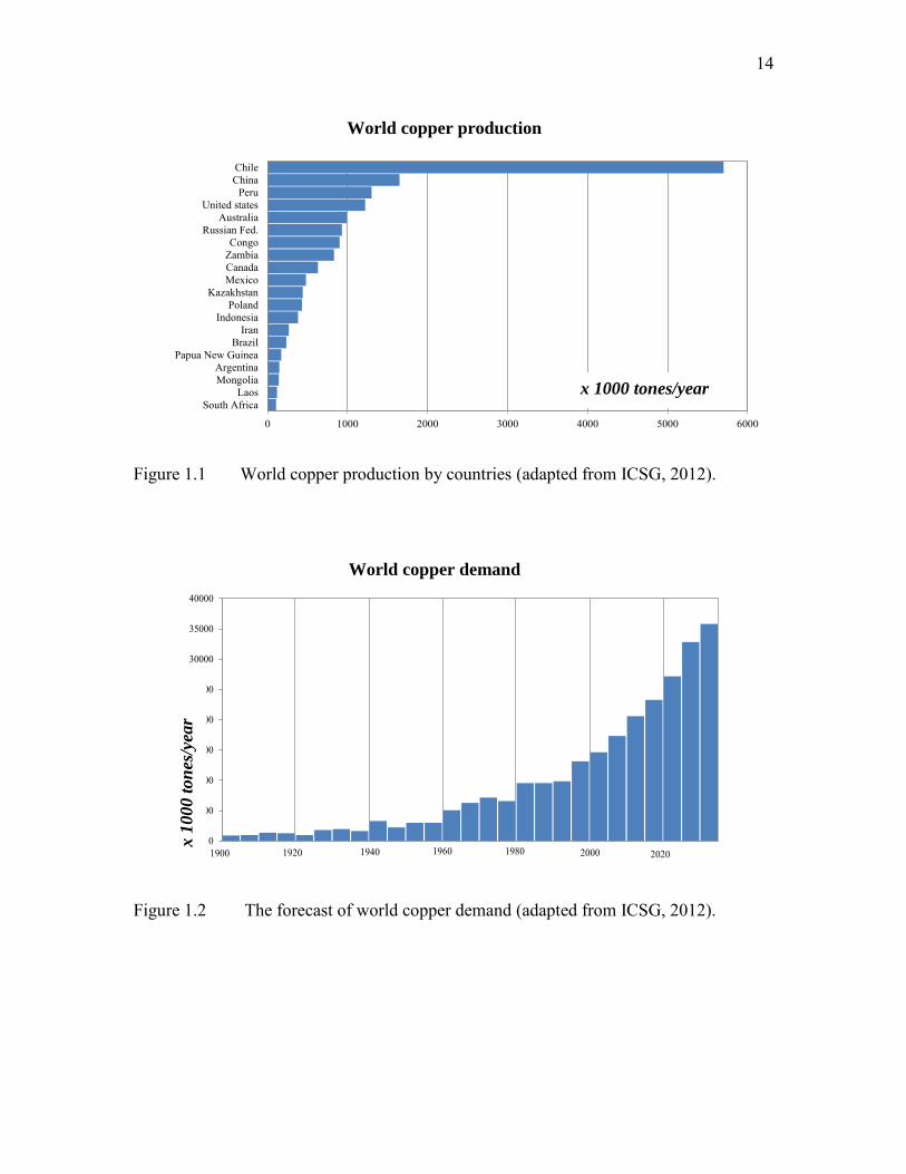
1.1 World copper production by countries (adapted from ICSG, 2012) …………... 14 1.2 The forecast of world copper demand (adapted from ICSG, 2012) ………….... 14 1.3 Locations of copper porphyry deposits of the world and metallogenic belts. Red
indicates Cu-Mo porphyry, blue – Cu porphyry, yellow – Cu-Au porphyry deposits (adapted from USGS, 2008) ………………………………………….. 15
1.4 Copper in reserves, resources, and past production in major copper discoveries by
country, 1999-2010 (adapted from SNL-Metals Economic Group, 2013) ……. 15 1.5 Location map of world-scale, large mineral deposits in Mongolia (adapted from
MRAM, 2012) ……………………………………………………………….... 16 1.6 Location map of Rio Tinto’s copper projects and operations around the world.
By-products may include gold, silver and molybdenum. Operations: 1-Escondida; 2-Grasberg; 3-Kennecott; 4-Oyu Tolgoi; Copper projects: 5-La Grange; 6-Resolution, 7-Bougainville (adapted from Rio Tinto Annual Report, 2013)…………………………………………………………………………… 16
1.7 Simplified process flow diagram of KUC’s Copperton concentrator (adapted from
KUC Annual Report, 2012) …………………………………………………… 17 2.1 A typical flow diagram used in the flotation of porphyry copper ores ………... 33 2.2 An illustration of the three main factors of flotation science and engineering
(adapted from Fuerstenau, 2007) ………………………………………….…… 33 2.3 Average molybdenum recovery according to particle size for the 18 months from
April 2005 until October 2006 at the Copperton plant. The curves are calculated based on analysis of weekly composites of feed and tails (Triffett et al., 2008)...34
2.5 Cross section of ore particles classified by mineral composition and exposed area
2.4 An example of a typical Andrews-Mika diagram (adapted from King and Schneider, 1998) …………………………………………….……………….… 34

xi
xi
(adapted from the work of Goodall et al., 2005)………………………….…….. 35 2.6 Schematic representation of the 2D scan of a polished section for liberation
analysis and the basis for the calculation of linear grade (adapted from the work of Miller and Lin, 1987) …………………………………………………………... 36
3.1 Results of copper (a) and molybdenum (b) recovery of batch flotation tests for
each ore type, at a grind target of 25% plus 100 mesh (FLSmidth, 2012) ..….... 58 3.2 The schematic flowsheet for sample preparation and subsequent characterization
analysis...……………………………………………………………………….. 59 3.3 Laboratory rod mill used for grinding calibration tests prior to liberation and
flotation testing...……………………………………………………………….. 60 3.4 Schematic diagram of the standard flotation test work including a detailed
characterization analysis ……………………………………………………….. 61 3.5 Particle size distributions of the LSE (a) and MZ2S (b) ore samples after grinding
for different times ……………………………………………….……………... 62 3.6 Grind calibration curve of the LSE, MZ2S and MZ2HE ore types ……………. 63 3.7 Cu and Mo recovery of the MZ2HE, LSE and MZ2S ore samples at different
grind fineness …………………………………………………………………... 64 3.8 MZ2HE ore: copper (red) and molybdenum (blue) flotation kinetics during
rougher flotation. Solid line represents coarse grinding at 35% +100 mesh and dashed line represents fine grinding at 25% -100 mesh …………...…………... 65
3.9 Illustration of typical form of grade/recovery curves for froth flotation based on
chemical analysis and rougher flotation kinetic data MZ2HE ore. Each curve represents the cumulative grade vs. the cumulative recovery for each time interval………………………………………………………………………….. 66
3.10 LSE ore: copper (red) and molybdenum (blue) flotation kinetics during rougher
flotation. Solid line represents coarse grinding at 35% +100 mesh and dashed line represents fine grinding at 25% + 100 mesh………………………………….... 67
3.11 Illustration of typical grade/recovery curves for froth flotation based on chemical
analysis and rougher flotation kinetic data of the LSE ore.…….……………… 68 3.12 Flotation kinetics of the MZ2S ore showing the relation between the Cu and Mo
recoveries with respect to the flotation time...………………………………….. 69 3.13 Illustration of typical form of grade/recovery curves for the rougher flotation of

xii
xii
the MZ2S ore ………………………………………………………………….. 70 3.14 Lost sulfide particles in the rougher tailings of the MZ2S ore sample;
photomicrograph by optical microscopy.……………………..…….…………. 71 4.1 Simplified X-ray beam, 𝐼0 attenuated through single (a) or multiple (b) materials,
having thicknesses, 𝑥A , 𝑥𝐵 results in attenuated beam,𝐼. Single – material (A); multiple – material (A and B). ……………………………………………....... 109
4.2 Mass attenuation coefficients of Al and Cu representing the gangue mineral
(quartz) and high density trace minerals (chalcopyrite and molybdenite) using software application called XMuDat (Nowotny, 1998) ………………….…… 109
4.3 The Xradia MicroXCT-400 system at the University of Utah. Major external
components: (A–Ergonomic station; B–EMO button; C–RESET button; D–light tower; E–enclosure; F-motion controller hardware; G–workstation; H-access door; J– power distribution; K– storage server) ………….………..……..…... 110
4.4 Visual internal view of the MicroXCT-400, with the access doors open: (A–
Safety lock; B–X-ray source; C–Sample stage; D–visual light camera; E–detector assembly; F- turret; G– macrolenses) ……….……….…………….…….…… 111
4.5 Photo of stacked Al and Cu foils (A) and radiographs of the stacked Al and Cu
wedges for DE calibration at 80 kV (B) and 140 kV (C) ……….….……..….. 112 4.6 Comparison between the measured step-wedge thickness and the reconstructed
thickness from DE radiography for the Al foil and Cu foil wedges ……..…... 112 4.7 DE radiographs (80 kV and 140 kV) of the quartz, aluminum, copper,
molybdenite, gold and lead samples for determination of the unknown coefficient and effective atomic numbers ………………………………….….…………. 113
4.8 Estimated (line) and measured (points) data of effective atomic numbers based on
the DE relative reflex of two radiographs, X .……………..………….……… 113 4.9 Microphotograph and radiographic image of main minerals (the detailed
information is in Table 4.5) in Cu-Mo flotation tailings for DE calibration at 80 kV and 140 kV: (1 – molybdenite; 2 – galena; 3 – bornite; 4 – chalcopyrite; 5 – azurite; 6 – pyrite; 7 – hematite; 8 – sphalerite; 9 - quartz) …….….……….... 114
4.10 Partial volume effect dilutes the X-ray intensity values of a mineral during
radiography analysis. In the case of MoS2, the resulting attenuated value is close to that of copper minerals, making it difficult to distinguish MoS2 from the other medium density and/or atomic number minerals ..…………………..……..… 114
4.11 Dependence of the effective atomic number upon radiography reflexes in the

xiii
xiii
regions of the photo effect and Compton scattering. The experimental dependence for materials of known composition are indicated..…………………..…..…… 115
4.12 Calibration curve for given 𝐾𝑖 and p=3.8 values and comparison between
estimated (blue) and actual (red) effective atomic numbers from DE radiographs for each mineral …………..…………………………………………………... 115
4.13 Histogram of the relative reflex of the most common sulfide minerals in the KUC
flotation tailings..………………………………………………………....…… 116 4.14 Molybdenite and chalcopyrite particles identified for each section of slide based
on DE radiography and optical inspection for the search and isolation of trace mineral particles .……………………………………………………...………. 117
4.15 Photo of cubic Cu ore particles (a) and the corresponding DE radiographs (b)..118 4.16 Sulfide mineral grains are identified from the estimated Cu minerals using DE
radiography. Most of these mineral grains are less than 0.2 mm …………….. 118 4.17 Comparison of the cubic Cu ore particles (3x3x3 mm) using DE radiography
(from Figure 4.15) and 3D tomography, respectively.…………..…….…...…. 119 4.18 Combination of DE radiography and detailed characterization analysis for mineral
properties …………………………………………………………………….... 119 4.19 DE radiography scans from the LSE rougher tailings (fine grinding – 25 % + 100
mesh size class). a) coarse size class; b) medium size class. The images on the right are low-energy (80kV), and the images on the left are high-energy (140kV)…………………………....……………………..…………...……….. 120
4.20 ImageJ thresholding function that segments the background and medium/low
atomic number minerals from high atomic number minerals. a) Threshold dialog box; b) image of molybdenite particles prior to tresholding; c) threshold adjustment to match particles; d) final binary threshold image showing black particles on white background ………………………………………...……… 121
4.21 Summary of rapid scan dual energy (DE) radiography and its application in the
analysis of tailings slides …….……………………………………………...... 122 5.1 A schematic diagram of the detailed characterization analysis of lost mineral
particles …..………………………………………...…………………………. 158 5.2 The values of each CT number for sulfide mineral phases at a voxel resolution of
5 µm (adapted from Medina, 2012) ..…………………………………………. 158 5.3 SEM backscattered images of chalcopyrite and molybdenite particles from

xiv
xiv
rougher concentrate for the MZ2HE ore. a) 300x150 µm; b) 150x75 µm ….... 159 5.4 SEM backscattered images of locked chalcopyrite particles (150x75 µm) from
rougher tailings for the MZ2HE ore ………………………………………….. 160 5.5 SEM backscattered images of 300x150 µm and 150x75 µm molybdenite particles
from rougher tailings of the MZ2S ore …………………………………….…. 161 5.6 Copper and molybdenum loss in the rougher tailings of the MZ2HE ore ….… 161 5.7 Copper and molybdenum loss in the rougher tailings of the LSE ore ….…….. 162 5.8 Copper and molybdenum loss in the rougher tailings of MZ2S ore ……….…. 162 5.9 ImageJ 3D object counter plug-in. Image of particles counted as part of analysis
and data table generated by ImageJ. a) 3D object counter dialog box; b) image of molybdenite particles prior to tresholding; c) threshold adjustment to match particles; d) thresholded particles are numbered as shown to allow for exact measurement tracking of molybdenite particles; e) data table can be saved as .xls and imported into a spreadsheet software such as Excel ……….…………….. 163
5.10 Molybdenum distribution in the rougher tailings of the MZ2HE, LSE and MZ2S
ores, size classes – 150x75 µm and 300x150 µm ..………………………...…. 164 5.11 Reconstructed 3D rendered image of the packed bed of rougher tailings samples
(250x150 µm) with a voxel resolution of 4.59 µm from HRXMT scans. The figures on the left show a complete view of the original (a) and segmented (b) HRXMT reconstructed image. The images on the right show separated low, medium, and high atomic number minerals. Image crated with Drishti software..…………………………………………………………………...…. 165
5.12 3D projections (a) showing the cross cursor locating at a detected molybdenite
particle (b) a cross section containing molybdenite particles (dark blue) taken out from the 3D reconstructed image shown in Figure 5.12. Image crated with Drishti software ………………………………....……………………………...……... 166
5.13 SEM image and corresponding EDS spectra of un-coated (a) and coated (b)
molybdenite particle .………………………………………………………….. 167 5.14 SEM back scattered images of LSE molybdenite particles from: rougher
concentrate (a), rougher tailings (b). EDS spectra from the Spot # 1 and Spot # 2 indicating that slime minerals predominantly cover the molybdenite surface .. 168
5.15 Magnified and X-ray mapped SEM image (a) of Spot # 2; distribution map for three different elements, in this case Mo (yellow), Si (grey) and O (white), can be combined in a three-band image. Composite colors are produced where different combinations of the elements are present in different phases in the sample. The
xv
xv
EDS spectrum (b) indicates that slime minerals predominantly cover the molybdenite .…………………………………………………………...……... 169
5.16 SEM back scattered images of the MZ2S molybdenite particles from rougher
concentrate (a), and rougher tailings (b). The EDS spectrum (qualitative) from the region is shown in Figure 5.17 (b) indicating the heavily oxidized layer on the molybdenite. …………………………………………………...……………… 170
5.17 Magnified SEM micrograph of the molybdenite surface from Spot # 2 shown in
Figure 5.16. SEM back scattered electron micrograph of the surface of a molybdenite particle (150x75 µm), isolated from the MZ2S rougher tailings. The EDS spectrum from the region shown in (a) indicates that the molybdenite surface was entirely oxidized ..………………………………………………………... 171
5.18 SEM image and EDS of a selected chalcopyrite particle isolated from MZ2S
rougher tailings. The corresponding EDS spectrum from the region shown in (a) indicate that the chalcopyrite is strongly oxidized due to surface oxidation……………………………………………………………….……… 171
5.19 SEM image and EDS of a coarse molybdenite particle, isolated from MZ2S
rougher tailings ….……………………….………………………………..….. 172 5.20 A survey (full range) XPS spectrum of molybdenite particles isolated from the
MZ2S and LSE rougher concentrate and tailings ..…………………..………. 172 5.21 High resolution XPS spectra of Mo 3d and S 2s peaks (a) and S 2p peaks (b), on
the MoS2 samples isolated from the LSE and MZ2S samples ….…….…..….. 173 5.22 Summary of detailed characterization analysis of Mo loss in the MZ2S
sample…………………………………………………………………………. 174 B.1 The X-ray source dialog icon …………………………………………………. 193 B.2 The magnification icon in the XMController …….......………………………. 193 B.3 The acquisition setting, motion control, image control window ………..……. 194 B.4 The acquisition control setting in the continuous mode .……….....….………. 194 B.5 Image control setting …….………………...…………………………………. 195 B.6 Reference applying method …..………………………………………………. 195

xvi
xvi
LIST OF ABBREVIATIONS
DE Dual Energy
FLS FLSmidth USA, Inc
GDP Gross Domestic Product
HRXMT High Resolution X-ray Micro Tomography
ICSG The International Copper Study Group
KUC Kennecott Utah Copper
MLA Mineral Liberation Analyzer
MRAM Mineral Resources Authority of Mongolia
NDT Non-Destructive Technology
QEMSCAN Quantitative Evaluation of Minerals by Scanning Electron Microscopy
ROI Region Of Interest
SEM Scanning Electron Microscopy
SEM-EDS Scanning Electron Microscopy coupled with Energy Dispersive X-ray
Spectroscopy
ToF-SIMS Time-of-Flight Secondary Ion Mass Spectrometry
USGS U.S. Geological Survey

xvii
xvii
XPS X-ray Photoelectron Spectroscopy
XRF X-ray Fluorescence

xviii
xviii
ACKNOWLEDGEMENTS
I would like to express my sincere appreciation to Professor Jan D. Miller, advisor
and chair of the supervisory committee, for his help, remarkable support, guidance, and
encouragement during the course of this dissertation research. In addition, I would like to
thank Dr. Chen-Luh Lin for his advice, knowledge and patience. Thanks are also
extended to Dr. Raj Rajamani, Dr. Sivaraman Gurusvamy, and Dr. Michael Nelson, for
their positive disposition as members of the supervisory committee and their valuable
advice and comments on some aspects of this work.
Thanks are also extended to Phil Thompson, Perry Allen, Lorin Redden, mentors,
friends, and alumni of the Department of Metallurgical Engineering, University of Utah,
and employees of FLSmidth, USA. In addition, I would like to extend my appreciation to
Rio Tinto for providing the research grant for this study. Without their encouragement
and insistence to pursue graduate studies in this department, it would have been
impossible for me to have the courage to come to the University of Utah and start this
beautiful journey.
Lastly, the author would like to express his deepest gratitude and appreciation to his
family. Particular thanks are expressed to his wife, Uyansanaa Udanbor, for her love,
support, understanding, and tremendous patience.

1
CHAPTER 1
INTRODUCTION
The more efficient production and use of mineral resources is a major objective in our
sustainability efforts. Resource characterization, referred to as geometallurgy, is a critical
component for optimization of the mine-to-mill process, and now can be accomplished
with advanced instrumentation including, for example, particle size analysis, X-ray
fluorescence (XRF), X-ray diffraction (XRD), X-ray photoelectron spectroscopy (XPS),
scanning electron microscopy coupled with energy dispersive X-ray spectroscopy (SEM-
EDS) which includes quantitative evaluation of minerals by scanning electron
microscopy (QEMSCAN) and mineral liberation analyzer (MLA) and high resolution X-
ray micro tomography (HRXMT). Geometallurgy relates to the practice of combining
geology with metallurgy, to create a spatially or geologically based predictive model for
mineral processing plants (Bulled and McInnes, 2005). Sampling and geometallurgical
information is important for exploration, deposit evaluation, mine and production
planning, analysis of separation, process efficiency, etc. Improved sampling and
geometallurgical analysis can save millions of dollars in the effective utilization of our
mineral resources (Miller, 2012).

2
1.1 Copper production worldwide
Copper metal is generally produced from a multistage process, beginning with the
mining and concentrating of low-grade ores containing copper sulfide minerals, and
followed by smelting and electrolytic refining to produce a pure copper cathode.
The U.S. Geological Survey (USGS) provides information to the public and to policy-
makers concerning the current use and flow of minerals and materials in the world
economy. According to data compiled by the USGS (2012), world mine production of
copper was 16.5 million metric tons (mt) in 2011; world reserves are estimated to be 540
mt, or 36 years at the 2011 rate of production. In recent times, 20 countries have
produced approximately 87 % of the world copper production, which is displayed in
Figure 1.1. World copper production was dominated by Chile and the United States for
several decades and now increasing contributions have come from Peru, China, and
Indonesia over the past two decades.
In March 2014, The International Copper Study Group (ICSG, 2014) released the
2014 Statistical Yearbook, which showed world copper production and consumption and
revealing that the trends in global refined copper consumption are progressing at an
alarming state. The outlook for copper demand is greatly focused on China, where copper
consumption will grow as a consequence of the overall economic growth of China. For
example, by 2025, one billion people are projected to live in Chinese urban areas and 221
Chinese cities will have been built (Mckinsey Global Institute, March 2009). Along with
these massive increases, increased demand will be seen in buildings and infrastructure. It
means that one billion Chinese will have become consumers, salaries will have increased,
and domestic consumption will continue growing faster than the GDP. More consumers,

3
means more demand for: cars, appliances, garments, electronics, buildings and
infrastructure. In other words, what does it all mean? More copper will be needed.
Industrial production is not keeping up with copper consumption and recent
indications suggest that the estimates in Chinese consumption are very conservative. It
now appears that in the next 25 years, the world will need to produce as much copper as
has been produced in the history of humanity. Figure 1.2 presents evidence of world
copper demand compiled by ICSG between 1900 and 2030. Copper consumption
expanded at an annual pace of 10.1%. Surprisingly strong Chinese demand is prompting
investors to rethink their dour predictions for copper demand, but this demand is not the
only major factor to consider in the outlook for copper. The world is also beginning to
feel the impact of supply challenges. When it comes to the production of copper, the
industry is experiencing difficulties from various aspects of the production cycle:
Discoveries of high grade deposits are less frequent;
More underground mines are producing copper, at a smaller output capacity than
open pits;
There are greater country risks and infrastructure challenges (remote locations);
Average grades of the ore bodies are declining;
Funding for exploration is inadequate.
Figure 1.3 shows the distribution of known copper deposits of the world based on the
ICSG (2012) world copper factbook. Porphyry copper deposits are the world’s most
important source of copper and molybdenum, and can contain major quantities of gold,
silver and tin, with some porphyry copper deposits having by-products of platinum,
palladium and tungsten. Approximately 60% of the world’s copper and 95% of the

4
world’s molybdenum is sourced from porphyry copper deposits (SolGold annual report,
2013). Porphyry copper deposits are copper ore bodies that are associated with
porphyritic intrusive rocks and the fluids that accompany them during the transition and
cooling of magma to rock. According to SNL metals economic group data (2013), 100
significant copper discoveries have been reported so far in the 1998-2012 period,
containing almost 395 million tons of copper.
Benefiting from the largest share of the discovery-oriented exploration budgets over
this period, Latin America hosts more than half of the discovered copper, followed
distantly by North America, Africa, Asia, Australia-Pacific, and Europe. Overall, the
industry found more copper in these significant discoveries than it produced; however,
the economic viability of new resources is influenced by factors such as location and
politics, capital and operating costs, and market conditions that inevitably reduce the
amount of copper that reaches production. To date, only about one-tenth of the copper in
these 100 discoveries has been converted to reserves with only 15 deposits having
reached production. According to the SNL-Metals economic group annual report (2013),
copper discoveries in reserves, resources, and past production in major copper
discoveries by country during 1999-2010 are presented in Figure 1.4.
1.2 Mongolian copper production
One promising location for copper production is in Mongolia, in the South Gobi
Desert, east of the Omnogovi province, where the Oyu Tolgoi deposit is located, one of
the world’s largest and richest copper porphyry deposits. Commercial operations began in
mid-2013 and Oyu Tolgoi’s open pit is now operating at full capacity under management

5
by Rio Tinto. In 2013, Oyu Tolgoi produced 77 thousand tons of copper and 157
thousand ounces of gold (Rio Tinto, 2013). Discussion of Mongolian copper production
is included because the dissertation research was supported by Rio Tinto. Mongolia is a
landlocked country in East and Central Asia, a fledgling democracy of just over 20 years
old, bordered by Russia and China. When Mongolia opened its doors to foreign
investment, major mining companies accepted the invitation and the incredible geological
riches buried beneath the soil became immediately apparent. Despite this influx, the
country's vast mineral resources remain largely unexplored and undeveloped. Mongolia
currently ranks among the top 10 resource-rich nations in the world. In Mongolia, the
mining sector plays a key role in industry and for the last few years, its output has been
driving the country’s economy. The mining sector’s share in the GDP reached
approximately 29.0 % in 2011 (MNSO, 2012). According to the Mongolian National
Statistical Organization (NSO) monthly report (2012), mineral exports accounted for 89
% of the total exports. The largest exported product was coal, accounting for 43.4 %,
followed by copper concentrate (19.1 %), crude oil (7.7 %) and gold (2.8 %). In terms of
major destination countries of export, China imported 92.6 % of the total exports from
Mongolia, followed by Russia (1.8 %). The real quantity of Mongolia's mineral resources
cannot yet be known. Mongolia’s vast territory has a great potential to hold rich mineral
deposits, including gold, copper, coal, fluorspar, silver, and uranium. Only 24.8% of the
Mongolian territory has been covered by general mineral exploration. There are over
8,000 individual mineral deposits in Mongolia, containing a wealth of over 440 different
minerals. Of these, around 600 deposits and outcrops have been fully explored and their
extent determined. These include over 180 gold deposits, 6 copper deposits, a lead

6
deposit, 5 tin deposits, 10 iron deposits, 4 silver deposits, 42 deposits of brown and
coking coal, 42 fluorspar deposits, 12 salt and 10 sodium sulfate deposits, 6 semiprecious
stone deposits, 9 crystal deposits and over 200 deposits of minerals used in the
production of construction materials, as well as a wealth of rare-earth metals. By 2011,
well over 200 deposits were already being exploited (MRAM, 2011). Figure 1.5 presents
the location of the largest copper and other mineral deposits mapped by the mineral
resources authority of Mongolia (MRAM).
Rio Tinto is a leading global mining and metals company, involved in every stage of
mineral and metal production, and is applying international best practices to the Oyu
tolgoi project. Rio Tinto is a major shareholder in the Oyu Tolgoi project. On October 6,
2009, Rio Tinto signed a long-term, comprehensive Investment Agreement with the
government of Mongolia for the construction and operation of the Oyu Tolgoi copper-
gold mining complex. The agreement creates a partnership between the Mongolian
government, which acquired a 34% interest in the project, and Turquoise Hill Resources,
which retained a controlling 66% interest in Oyu Tolgoi. Global miner Rio Tinto, which
joined Turquoise Hill Resources as a strategic partner in October 2006, is managing the
development of Oyu Tolgoi. This includes world-class health and safety standards and a
commitment to sustainable development and operational excellence. The Oyu Tolgoi
project is the largest financial undertaking in Mongolia's history, and working in
partnership with the government of Mongolia, Rio Tinto has striven to ensure the proper
training and preparation of the Mongolian workforce with the goal of developing a strong
workforce for Mongolia’s future mining industry. Participants are also given a wide
range of skills that will build and support a diverse economy. All of the copper projects

7
and operations of Rio Tinto are depicted in Figure 1.6. Rio Tinto Copper group has
operating assets around the world - Kennecott, Oyu Tolgoi, Escondida and Grasberg –
and two world-class greenfield projects, Resolution and La Grange. The general
characteristics of alteration, mineralization, and geological settling of the Kennecott
Bingham Canyon deposit and the Oyu Tolgoi deposit are quite similar and froth flotation
is the main method of separating copper minerals from gangue for both operations.
1.3 Significance of flotation
Froth flotation is the most common technique used in beneficiation of complex-
structured, valuable sulfide minerals such as chalcopyrite, galena, sphalerite and silver.
The importance of froth flotation has long been, and continues to be, an important aspect
of the mining industry, especially for metallurgical engineers. The flotation of sulfide
minerals, such as chalcopyrite (CuFeS2), chalcocite (Cu2S), covellite (CuS), pyrite
(FeS2), galena (PbS) and sphalerite (ZnS), has been practiced successfully for over 100
years (Fuerstenau, 2007). The trend in the copper mining industry of today is that the
total recovery of copper and associated metals in the entire process of copper production
must be optimized. Optimum sulfide mineral recoveries have always been a problem
because there are continuous changes in the properties of the plant feed. Tabulations of
operating data also reveal some of the technical problems associated with the flotation of
sulfide ores. For example, the average recovery of copper in the world flotation plants
was reported to be only 82%, and only 58% recovery of the associated molybdenum
(Herrera-Urbina, 2003). For meaningful improvement, new and better technology must
be developed to increase recovery. During normal operations, sulfide mineral flotation is

8
generally satisfactory. However, the flotation response changes due to variations in the
feed characteristics in an operating plant. These result in fluctuations in the concentrate
grade and sometimes the recovery will be low with a significant loss of base and precious
metals. Froth flotation is affected by many parameters that are beyond the control of a
mineral processing engineer. As is well known, liberation of the valuable minerals is
necessary for successful flotation separations. Beyond liberation, process variables such
as slime coating, surface oxidation, pH, conditioning time, type of reagents (collectors,
frothers, depressants, activators) and also their dosage can significantly influence the
success of the flotation separation, which in turn, determines the grade and recovery of
the metal in the concentrate. These factors must be considered in an attempt to determine
their significance on the separation efficiency. In particular, the identification and
characterization of lost (trace) particles in the flotation tailings of a copper porphyry ore
must be studied. In particular, in this dissertation research the identification and
characterization of chalcopyrite and molybdenite particles lost to the tailings during the
flotation of Bingham Canyon ore will be studied. Babcock et al. (1997) describe the
Bingham Canyon deposit as a classic porphyry copper deposit exhibiting concentric
zones of alteration and mineralization.
1.4 Flotation at the Copperton concentrator
Kennecott Utah Copper (KUC), a wholly owned subsidiary of Rio Tinto, operates the
Bingham Canyon mine, one of the world’s largest open pit copper mines. The mine and
associated Copperton concentrator are located approximately 26 miles southwest of Salt
Lake City, Utah, in the eastern foothills of the Oquirrh mountain range near the city of

9
Copperton. The deposit is notable for its size, containing premining reserves of nearly 3
billion tons of ore at 0.67% copper (USGS, 2011). Nested within the copper ore body are
overlapping zones of molybdenum, gold and silver containing 0.1% molybdenite (MoS2),
0.3 g/t gold and 1.5 g/t silver (Triffett and Bradshaw, 2008).
In general, the main sulfide minerals are chalcopyrite, bornite, molybdenite, and
pyrite. The major gangue mineral is quartz. According to Babbock et al. (1997) and
Nelson (2007), the Bingham Canyon deposit contains a number of ore types that are
classified based initially on lithology and on processing characteristics. The quantity of
ore processed through the concentrator each day requires that several ore types will be
treated at once, in a blend. The processing characteristics of individual ore types have
been extensively modeled and these are arithmetically combined to estimate the expected
performance of blends in the production planning process.
A brief plant description (Triffett and Bradshaw, 2008) is presented in the following
paragraphs in order to understand the overall process and the relevance to this
dissertation research. Processing of the ore is performed on-site using crushing, grinding,
and flotation to recover copper and molybdenum concentrates. A simplified process flow
diagram of KUC’s Copperton concentrator is provided in Figure 1.7.
The run of mine ore is crushed with a gyratory crusher and then reduced to less than
100 mesh (150 µm) by wet grinding using semi-autogenous grinding (SAG) mills and
ball mills. The grinding operation consists of three parallel SAG mills, and two ball mills
corresponding to each SAG mill. The SAG mill discharge is screened on vibrating
screens and the coarse material from the screen is sent back for crushing in a cone crusher
(MP1000). The product of the cone crusher is returned to the SAG mill for further

10
grinding. The ball mill ground product is classified in cyclones of 26 inches for achieving
a product size of 80% passing 100 mesh (150 µm). The cyclone overflow from the
grinding circuit is combined and distributed equally to 4 parallel rougher-scavenger
flotation lines containing 11 Wemco flotation cells (3000 ft3/cell) per line. The rougher-
scavenger residence time is approximately 15 minutes. The rougher concentrate is
reground to 74 % passing 200 mesh (74 µm) and is further processed in a cleaner circuit
with conventional mechanical cells. The cleaner circuit produces a final bulk concentrate.
The bulk concentrate is further sent for separation of copper from molybdenum by
depressing the copper minerals using sodium hydrosulfide (NaSH) as a depressant. The
average plant recovery is usually between 80 % and 90 % for copper, and molybdenum
recovery may range between 65 % and 85 % (Crozier, 1979). Tailings are sent to
thickeners for water recovery and the thickened slurry is transported by a 48 inch pipeline
to the tailings impoundment area. The copper concentrate is transported by pipeline for
filtration. The molybdenum concentrate is filtered, dried and packed in bags at the
Copperton site (Zanin et al., 2008).
1.5 Research objectives
The objectives of the dissertation research were to investigate the significance of
problems associated with the flotation efficiency for selected KUC ore types.
Specifically, the research included the following objectives:
Evaluation of the flotation response for different ore types;
Development of a rapid scan methodology using radiography to identify, isolate,
and collect lost sulfide mineral particles from the flotation tailings;

11
Examination of the liberation and the surface chemistry characteristics of lost
particles using advanced analytical techniques such as HRXMT, XPS, SEM, ToF-
SIMS and/or QEMSCAN;
Determination of the extent to which surface chemistry, exposure/liberation and
slime coating considerations contribute to the loss of sulfide mineral particles in
the tailings.
Modern instrumentation and equipment were used for characterization of feed and
flotation products. Based on the most significant limitation to flotation efficiency, future
flotation experiments should be carried out to evaluate possible alternatives for improved
flotation recovery of copper (Cu) and molybdenum (Mo).
The variability of the feed quality delivered to flotation plants in mining operations
can provide challenges to the operational staff in attempting to achieve satisfactory
recovery and grade efficiency. When faced with variables or difficult ores, plant
operators are often required to implement operational parameter changes to maintain
flotation efficiency. This research was aimed at improving the understanding of the
factors affecting the flotation efficiency of copper and molybdenum minerals from
porphyry copper ores and providing some possible solutions to these challenges.
Specifically, the identification and characterization of lost chalcopyrite and molybdenite
particles using a dual energy rapid scan radiography method for the analysis of flotation
tailings was considered. Of course, working with tailings is never easy. Minor or trace
concentrations of valuable elements or minerals means that sample collection and
integrity become one of the major concerns in any project relating to the tailings.
Research findings can be used for many applications such as fast geometallurgical

12
analysis, including identification of mineral zones from drill core samples and the search
and isolation of trace mineral particles from the feed and tailings streams. Preliminary
results verified that dual energy radiography works well to fulfill this function.
1.6 Dissertation organization
After the introduction in Chapter 1 and the literature review in Chapter 2, the
dissertation research consists of three main aspects. The first part of Chapter 3 involves
laboratory flotation experiments and variables that affect the flotation separation
efficiencies are discussed with the aim of increasing copper and molybdenum flotation
efficiencies. Later in Chapter 3, research results from batch flotation testing are reported
regarding the loss of sulfide particles such as chalcopyrite and molybdenite that exists in
copper flotation circuits of milling plants that treat porphyry copper ores. Results of
rougher flotation conducted for several ore types of KUC are reported. The rougher
flotation testing was controlled by changing the grind fineness and slime coating.
The second part of this dissertation research, presented in Chapter 4, was to develop a
rapid scan methodology using 2D radiography to identify, isolate, and collect lost sulfide
mineral particles in flotation tailings. In Chapter 4, the theory and procedures for rapid
scan dual energy (DE) 2D radiography are described for the evaluation and isolation of
trace mineral particles from samples at the ppm level. During radiography analysis, the
flotation tailings samples are split into narrow size fractions, each size fraction
distributed/assembled on projection plates, and then the plates placed in the sample
holder of the X-ray instrument for irradiation at two energy levels (dual energy analysis).
In this way, for example, more than 40,000 particles, 150x75 µm in size can be

13
interrogated in less than 15 minutes for identification of particles containing high and
medium density mineral phases and their composition can be estimated.
The third part of this dissertation research is presented in Chapter 5 and is concerned
with the characterization of lost tailings particles including the liberation and the surface
chemistry characteristics of lost particles using advanced techniques such as HRXMT,
SEM and XPS. Based on characterization results of advanced instrumentation, the extent
to which surface chemistry, mineral exposure/liberation and slime coating contribute to
the loss of sulfide mineral particles in the tailings are determined. Detailed results and
recommendations will be presented in Chapter 5.
Finally, Chapter 6 presents a summary and general conclusion from research findings
regarding the flotation characteristics of the KUC samples and their impact on flotation
plant efficiency.
14
Figure 1.1 World copper production by countries (adapted from ICSG, 2012).
Figure 1.2 The forecast of world copper demand (adapted from ICSG, 2012).
0 1000 2000 3000 4000 5000 6000
ChileChina
PeruUnited states
AustraliaRussian Fed.
CongoZambiaCanadaMexico
KazakhstanPoland
IndonesiaIran
BrazilPapua New Guinea
ArgentinaMongolia
LaosSouth Africa
World copper production(' 000 tonnes/year by refined copper)
0
5000
10000
15000
20000
25000
30000
35000
40000
World copper demand(' 000 tonnes/year )
1900 1920 1940 1960 1980 2000 2020
x 1000 tones/year
World copper production
x 1
000 t
on
es/y
ear
World copper demand

15
Figure 1.3 Locations of copper porphyry deposits of the world and metallogenic belts. Red indicates Cu-Mo porphyry, blue – Cu porphyry, yellow – Cu-Au porphyry deposits (adapted from USGS, 2008).
Figure 1.4 Copper in reserves, resources, and past production in major copper discoveries by country, 1999-2010 (adapted from SNL-Metals Economic Group, 2013).

16
Figure 1.5 Location map of world-scale, large mineral deposits in Mongolia (adapted from MRAM, 2012).
Figure 1.6 Location map of Rio Tinto’s copper projects and operations around the world. By-products may include gold, silver and molybdenum. Operations: 1- Escondida; 2 – Grasberg; 3 - Kennecott; 4 - Oyu Tolgoi; Copper projects: 5 - La Grange; 6 –Resolution; 7-Bougainville (adapted from Rio Tinto Annual Report, 2013).

17
Figu
re 1
.7
Sim
plifi
ed p
roce
ss f
low
dia
gram
of
KU
C’s
Cop
perto
n C
once
ntra
tor
(Dat
a so
urce
: Ken
neco
tt A
nnua
l Rep
ort,
2012
).
Mo f
lota
tion
SA
G #
4
Cyc
lon
e fe
ed
Ball
mil
l &
Cyc
lon
es
New
pla
nt
Old
pla
nt
Fee
d b
ox
Fee
d b
ox
Flo
tati
on
row
Flo
tati
on
row
Reg
rin
d m
ill
Reg
rin
d m
ill
Rou
gh
er
Cle
an
er
Cle
an
er
Sca
ven
ger
Mec
han
ical
scave
nger
Mec
han
ical
scave
nger
Cu
/Mo
thic
ken
er
Fin
al
Mo
thic
ken
er
Fin
al
Cu
thic
ken
er
SA
G #
1
SA
G #
2
SA
G #
3
Cyc
lon
e fe
ed
sum
p
Cyc
lon
e fe
ed
sum
p
Cyc
lon
e fe
ed
sum
p
To r
oast
er
To s
mel
ter
To t
ail
ings
du
m
Fro
m
pri
mary
cru
sher

18
CHAPTER 2
FLOTATION OF COPPER-MOLYBDENUM ORES
2.1 Introduction
Froth flotation is a key unit process in the recovery of most of the world’s copper,
lead, molybdenum, nickel, platinum group elements, silver, and zinc, and in the treatment
of certain gold and tin ores. Flotation for the recovery of copper sulfide minerals has long
been, and continues to be, of significant importance to the mining industry, especially to
metallurgical engineers. Flotation is the preferred method for the recovery of most sulfide
minerals. The flotation of sulfide minerals, such as chalcopyrite (CuFeS2), chalcocite
(Cu2S), pyrite (FeS2), galena (PbS) and sphalerite (ZnS), has been practiced for over 100
years (Fuerstenau, 2005). Bulatovic (2007) reported that copper ores can be divided into
the following groups with regard to processing:
Copper sulfide ores, where the pyrite content can vary from 10% to 90%. Some
copper sulfide ores also contain significant quantities of gold and silver.
According to mineral composition, these ores can be subdivided into three main
groups including (a) copper–gold ore, (b) copper sulfide ore with moderate pyrite
content and (c) massive sulfide copper ores;
Copper porphyry ores are the most abundant copper ores; these ores most often

19
contain molybdenum, which is recovered as a by-product. More than 60% of the
world’s copper production and approximately 90 % of the world’s molybdenum
production comes from copper porphyry ores.
Copper (Cu) and molybdenum (Mo) usually occur as chalcopyrite (CuFeS2) and
molybdenite (MoS2) minerals in copper porphyry ores and are usually associated with
pyrite (FeS2) and silicate gangue minerals. These Cu and Mo sulfide minerals are
generally recovered by froth flotation (Fuerstenau and Herrera-Urbina, 1989). During
flotation, some amounts of Cu and Mo are lost to tailings streams, as these metals may be
entrapped in gangue materials and remain unliberated, may be present as fine slimes, or
may report to tailings due to problems in process operations. For example, the average
recovery of copper in US flotation plants was reported to be only 82%, with only 50 – 85
% average recovery of the associated molybdenum (Herrera-Urbina, 2003). Huge
amounts of such tailings are generated at many copper porphyry mines around the world.
Due to the increased utilization of Cu and Mo in many industries and the rapid
depletion of existing ore deposits, development of new deposits will continue to receive
further attention (Herrera-Urbina, 2003).
The application of flotation to concentrate valuable minerals is environmentally
friendly and economically feasible since generally the ore has been reduced to a
liberation size suitable for flotation. However, when the size becomes too fine other
challenges, such as surface oxidation and slime coating may affect the flotation
separation variables, including collector/frother selections and concentrations, extent of
surface modification by attrition or addition of promoters and depressants, among others
(Bulatovic, 2007).

20
Flotation properties of individual copper minerals and associated sulfides such as
chalcopyrite, bornite, molybdenite, and pyrite from natural ores differ significantly.
These differences are briefly described in some textbooks, for example, in Bulatovic
(2007). The mineralogy of the ore, mineral impurities in a crystal structure, variation in
crystal structure, other interfering gangue minerals, and the liberation characteristics of
individual minerals in a particular ore are some of the factors that influence the efficiency
of the flotation separation.
2.2 Reagent schemes in the flotation of copper porphyry ores
The factors which determine a reagent schedule and flow diagram for porphyry
copper ores include ore nature and mineralogy, flotation behavior of gangue minerals,
what minerals are present, the amount and occurrence of pyrite and the presence of clay
in the ore. A typical flow diagram used in the flotation of porphyry copper ores is shown
in Figure 2.1. Reagent schemes used for the treatment of porphyry copper ores are
relatively simple and usually involve lime as a modifier, xanthate as the primary
collector, and a secondary collector that includes dithiophosphates, mercaptans,
thionocarbamates and xanthogen formates. The next important issue is separation of the
Cu–Mo rougher concentrate. In this research, rougher flotation of Cu-Mo is considered
rather than the separation of Mo from the copper rougher concentrate.
2.3 Factors affecting the flotation recovery of copper porphyry ore
Due to the many variables that influence flotation and affect the process of
mineralization of air bubbles, considerable attention has been given to the development

21
of sulfide flotation technology in the past century (Maksimov and Emeljanov, 1983; Xu
and Changlian, 1985; Szatkowski and Freyberger, 1985a,b; Vanangamudi and Rao, 1986;
Lazic and Calic, 2000; Brozek and Mlynarczykowska, 2006). Unfortunately, because
froth flotation is a complex engineering system, incorporating several highly interrelated
parameters such as chemistry, operational performance and equipment, (see Figure 2.2),
it is a difficult process to study. Changes in one setting will inevitably cause a demand for
changes in other parts of the system. Therefore, isolating the effect of a single factor
becomes problematic. For meaningful improvement, new and better technology must be
developed to increase the recovery. During recent years, the mining industry has focused
on implementing new technologies such as equipment, expert control systems and new
chemical reagents in order to increase the operational performance of the flotation
circuits. Optimum sulfide mineral recoveries have always been a problem because there
are continuous changes in the properties of plant feed. Of course, the development of new
ore deposits generally requires special attention to establish appropriate reagent schedules
and operating conditions.
The focus of this dissertation will be on the operational features such as
characterization of lost particles in the tailings, including mineral exposure/liberation,
slime coating/aggregation, and surface chemistry issues. A better understanding of these
factors is an important key to achieving improved flotation recovery (Roman, 2008). The
process of flotation is a sequence of several steps, some of which are done in the ore
preparation stage and some in the flotation cell itself (Harris, 1976; Klimpel et al., 1986).
From a survey of the literature, it has been observed that following sequence is followed
for the processing of copper ore:

22
Liberation of desired material (using ore preparation methods such as crushing
and grinding);
Adsorption of reagents on particle surfaces through conditioning (conditioning of
the slurry done with appropriate reagents);
Generation of air bubbles (injection of finely disseminated air bubbles through the
slurry);
Collision of particles with bubbles and their attachment;
Generation of an air-water-mineral aggregation in the presence of reagents;
Transport of the air-water-mineral aggregate to the surface.
Laboratory experimental results are used to evaluate particle characteristics and their
response to flotation. These tests are also useful in improving the existing process in
operating plants through evaluation of possible changes, including reagent schedules,
aeration, cleaning steps and regrinding (Roman, 2008).
Leja (1982), Shirley and Sutulov (1985), Raghavan and Hsu (1984), Triffett and
Bradshaw (2008), Triffett et al. (2008), and Zanin et al. (2009) summarized a number of
difficulties encountered in the treatment of Cu and Mo minerals in the flotation process
and these difficulties can be grouped under the following headings:
Effect of mineral exposure and liberation (especially if there is a high degree of
interlocking and fine dissemination of the valuable sulfides within the gangue
matrix);
Effect of particle interactions (the coexistence and attachment of hydrophilic clay
minerals producing interference, and coexistence of hydrophobic gangue minerals
such as talc, graphite, and other carbonaceous minerals);

23
Effect of surface and pulp chemistry (surface oxidation, coexistence of sulfide and
oxidized minerals such as oxides, carbonates, and sulfates, and the effect of
dissolved ions and residual reagents).
Few reports are available addressing all of the above limiting characteristics on the
recovery of sulfide minerals. In the present study, attempts are made to understand the
significance of mineral exposure/liberation, slime coating and surface chemistry in the
flotation of difficult-to-float ore types from the Bingham Canyon deposit, KUC. These
factors will be discussed in more detail in the next sections.
2.3.1 Particle size
Particle size is one of the most important parameters in flotation and its significance
in the flotation process was recognized early on (Trahar, 1981). It was generally found
that for a particular flotation system there is an optimum particle size range, usually 10–
100 μm, where high flotation response and efficiency are observed. Outside this range,
recovery drops significantly (King, 1982; Klimpel and Hansen, 1988). The result is a
curve between flotation recoveries vs. particle size, resembling an inverted U shape. The
particle size range, in turn, affects response to flotation variables. For instance, due to
lower mass and inertial force, fine particles exhibit low collision efficiencies. On the
other hand, maximum floatability for coarse particle size is determined by the detachment
process. There have been many studies conducted to investigate the positive and negative
effects caused by fine and coarse particles in flotation efficiency (Santana et al., 2008;
Muganda et al., 2011). Triffett et al. (2008) investigated the particle size vs. recovery for
molybdenite and copper in the rougher flotation circuit, which are routinely measured on

24
the weekly production composites at the Copperton plant, KUC. Figure 2.3 presents the
average size vs. recoveries of Cu and Mo for the 18 months from April 2005 until
October 2006 at the Copperton plant.
As can be seen in Figure 2.3, both metals display a recovery curve according to
particle size with the maximum recovery being achieved in the intermediate size fractions
and the coarse and fine particles being recovered at a lower rate (Triffett et al., 2008). In
addition, Triffett and Bradshaw (2008) found that the recovery of molybdenite peaks in
the 38 to 75 µm size range, while the copper recovery is high across a broader range of
sizes from 38 to 106 µm. The recovery of molybdenite also drops to a greater extent than
the copper in the coarse and fine sizes. Raghavan and Hsu (1984) reported that the effect
of particle size on the kinetics of flotation can be explained as follows:
Theoretically, the larger particles of molybdenite are characterized by a much
higher face-to-edge ratio and hence are likely to exhibit better floatability;
For smaller particles, which possess a lower face-to-edge ratio, the face-to-edge
ratio and charge established by the broken bonds on the edges will play a decisive
role. Increased particle charge due to smaller particles sizes leads to cohesion,
agglomeration and segregation.
2.3.2 Mineral liberation/exposure
The efficiency of sulfide mineral flotation is controlled by another important variable,
mineral liberation. Basically, liberation is the release of valuable minerals from waste
gangue minerals during comminution and is desired to happen at the coarsest possible
particle size. In practice, complete liberation is seldom achieved, even if the ore is ground

25
to the desired particle size. Of course, some degree of liberation is necessary if separation
and concentration are to be achieved in mineral processing operations. The degree of
liberation is expressed as the percentage of the mineral occurring as free particles, in
relation to the total mineral content, in the particle population. The degree of liberation is
typically based on the volume percent of the desired mineral grain in a whole particle.
Generally, mineral liberation characteristics are described in several ways:
Mineral locking indicates weight % of the given phase, which is associated with
other phases in composite particles;
Mineral liberation analysis by particle composition indicates the weight
percentage of a given phase in a given liberation class. For example, the fraction
of the mineral in the liberation class, 95-100 %, describes particles composed of
95 weight % of Cu sulfide mineral and 5 weight % of gangue minerals up to
liberated particles of 100 % copper sulfide minerals;
Mineral exposure analysis indicates a fraction of grains exposed for a given
particle size class.
Since flotation is based on particle surface features, not all locked particles have an
equal chance to float. Locked particles that contain 50 % copper sulfide mineral may
float very well if the particle surface consists exclusively of the copper sulfide mineral.
On the other hand, the opposite may be true and a composite particle containing 80 %
copper sulfide may not float at all. The surface composition is more important than the
extent of liberation.
Several attempts have been made to quantitatively estimate the degree of liberation as
a function of particle size. The foundation for liberation prediction models is the

26
Andrews-Mika diagram, which describes what type of progeny particles will be
generated when a single particle breaks during comminution (King and Schneider, 1998).
An example of an Andrews-Mika diagram is illustrated in Figure 2.4.
Models for liberation prediction developed by King and Schneider (1998), Schneider
(1995; 2003), Davy (1984), Gay and Latti (2006), Miller and Lin (1988; 2004, Miller et
al. (2009), Lin et al. (1987; 2001; 2013) and Goodall et al. (2005) are based on mineral
composition and texture analysis.
Basically, these models were developed for binary systems and they may not apply to
multiphase ores, and all prediction models rely on 2D polished section measurements and
3D estimations based on stereological correction. In 2D, the degree of mineral liberation
is done by two methods: an area method or a linear intercept method (Lin et al., 1987). In
either case, the 2D analysis will overestimate the extent of liberation. Figure 2.5 presents
the cross section of ore particles classified by mineral composition and exposed area. The
flotation of sulfide minerals requires a highly exposed surface area of the minerals to
improve the interaction and dispersion of reagents on the mineral surface. Thus, the
exposed surface area also has a significant impact on the sulfide recovery by flotation.
In 2D, the exposed surface area can be associated with the perimeter exposed and the
area of the mineral on the particle. The combination of these geometrical properties can
be used for the calculation of the mineral exposure factor, ( MEF ), which can be defined
as (Roman, 2008):
𝐴𝑖 = ∑(𝐴𝑖𝑃𝑖
𝑖=1
100𝑛⁄ )
(1)

27
where 𝑛 is the total number of particles, 𝐴𝑖 is the percent area and 𝑃𝑖 is the percent
exposed perimeter of the mineral in the particle. The maximum value of MEF
corresponds to 100 %, which is equivalent to a fully liberated mineral. For a population
of particles, the area and perimeter are calculated for each mineral in each particle by
optical microscopy and/or SEM with image analysis software.
There have been several systems developed in the past for mineral liberation analysis
(Lin et al 1987; Roman, 2008). However, previous industrial applications of liberation
data have been limited because data acquisition has been difficult, expensive and time
intensive. Recent advances in technology, especially in electronics and computing, have
allowed for the development of accurate, fast and user friendly mineral liberation
analytical techniques. Basic instrumentation used for evaluating mineral liberation and
mineral exposure characteristics include: optical microscopy, transmitted and reflected-
light microscopy (Gribble and Hall, 1992), and SEM equipped with energy dispersive
spectroscopy (EDS). Nowadays, the two SEM based automated image analysis systems
including QEMSCAN (Goodall et al., 2005) and the mineral liberation analyzer (Gu,
2003) are the most commonly used systems in mineral liberation studies. In either case,
the liberation analysis of polished sections overestimates the extent of liberation because
some sectioned particles can appear to be fully liberated, as is exemplified in Figure 2.6
In order to estimate the volumetric liberation from polished section analysis,
stereological models are applied. However, the stereological models are not satisfactory
because model parameters depend on the ore texture, which is unique for each ore type
(Miller and Lin 1988, 2004, 2013). Now, it is possible to make 3D X-ray
microtomography (XMT) measurements of liberation.

28
Such measurements and data analysis are presented in Chapter 5. High-resolution 3D
images revealing the internal structure of multiphase particulate samples can now be
obtained through modern techniques such as XMT (Garcia et al., 2009; Medina, 2012;
Hsieh, 2012,).
2.3.3 Particle-particle interactions
The difficulty of treating ores in the presence of clay minerals is well known in the
mineral processing industry. There have been several studies conducted to investigate the
negative effects caused by fine particles, which include surface coating (Raghavan and
Hsu 1984, Bulatovic, 2007; Triffet and Bradshaw, 2008; Zanin, et al., 2009; Peng and
Grano, 2010), increased reagent consumption due to the high surface area of clays (Guy
and Trahar, 1984), transferring large quantities of clay minerals into the concentrate,
increasing pulp viscosity, and changing froth stability. Bulatovic (2007) and Raghavan
and Hsu (1984) briefly explained that the presence of clay in copper porphyry ores causes
a loss in recovery, possibly due to the presence of slime coatings on mineral surfaces or
on air bubbles. Clay minerals such as talc, kaolinite, bentonite, and smectite, which are
often associated with copper, gold, and other valuable minerals, increase reagent
consumption and can create serious frothing/nonfrothing problems at the Copperton
concentrator. This phenomenon is discussed by Triffett et al., (2008), Zanin et al., (2009),
and Peng (2010), who noted that there have been numerous observations of these clay
minerals having a deleterious effect on mineral flotation grade, recovery, and pulp
viscosity. However, rigorous investigations on how clay minerals affect flotation are still
not available. Basically, major studies show that the slime coating of the mineral surface

29
occurs due to electrostatic attraction and explain that the fine clay particles are
electrostatically attracted to the surface of mineral particles and the attachment is heavily
dependent on the magnitude and sign of the zeta potentials of the mineral particles and
the fines (Arnold and Aplan, 1986).
The surface charges and electrophoresis mobility can be measured using a zeta
potential meter. Visual evidence for the presence or absence of slime coating can be
studied with the use of a scanning electron microscope (SEM).
Another important problem generated by the presence of slime is when the fine
particles of a gangue mineral adhere to each other by creating electrostatic and/or steric
repulsion forces, which counterbalance the contribution of the Van Der Waals attraction
to the total net force. Dispersants are widely used to modify the colloidal interactions
between gangue particles. These dispersants are mostly anionic polymers and adsorb on
mineral surfaces, making them more negative (Huynh et al., 2000). Classification
methods such as cyclones are more economical and efficient for separating fine particles
from coarse minerals (Greet and Smart, 1996). In addition, ultrasonic treatment can
disperse the clay particles, increase the flotation recovery, and reduce the required
collector dosage (Celik, 1988). Finally, the best and most economical way to treat these
types of ores is to blend them in a small proportion with normal ores.
2.3.4 Surface oxidation
Sillitoe and Petersen (1996) mentioned that the formation of copper ore bodies occurs
in the following way. Copper is dissolved deep underground and geothermal activity
brings the copper near surface environments to cool. Copper and associated metals then

30
precipitate into veins and disseminate within rock. Oxidation occurs as the deposits are
exposed to air or oxygen-rich water flowing over them. Oxidation in turn alters the
mineralogy. When sulfur is oxidized, it becomes soluble and is carried away in acid
solution, thus copper and iron sulfides are replaced by carbonates and oxides.
The flotation of copper sulfide minerals is intimately associated with their surface
oxidation. Extensive studies have been conducted to understand how oxidation influences
sulfide flotation behavior (Chander and Fuerstenau, 1974; Senior and Trahar, 1991).
Fullston et al. (1999) measured the zeta potential of copper sulfide minerals including
chalcocite, covellite, chalcopyrite, bornite, enargite and tennantite as a function of pH and
the oxidation condition. They found that chalcopyrite was the most electrochemically
noble while chalcocite was the most electrochemically active in terms of surface
oxidation. As mentioned by Senior and Trahar (1991), metal hydroxides on the mineral
surface decrease the flotation of copper sulfide minerals even in the presence of collector.
Barzyk et al. (1981) found that chalcocite surface oxidation had a strong effect on both
xanthate adsorption and chalcocite floatability, and the most oxidized chalcocite sample
required 100 times more collector consumption to obtain the same flotation results than
as the least oxidized sample. There is a strong relationship between copper recovery and
the electrochemical potential in flotation.
2.3.5 Process water influence
Because of its impact on the quality of human life and the environment, water
resource management has become an important issue in the world. Several research
studies indicate that recycling of process water is a potential option. Recycled process

31
water may be treated and then re-introduced into various sections of flotation operations
depending on its effect on mineral surface reactions (Broman, 1980; Forssberg et al.,
1985; Rao and Finch, 1989; Basilio et al., 1996; Leavay et al., 2001; Wei et al., 2006).
In mineral processing plants, the processed water is recycled from the tailings dams,
thickener overflows, and dewatering and filtration units. In these streams, the dissolved
ions, suspended solids and flotation reagents have insufficient time to decompose and
precipitate. In this case, the concentration of the contaminants can adversely affect
flotation performance. Typical contaminants in the process water are the colloid materials
(silicates, clays, precipitated metal hydroxides, etc.), ions of base metals, thiosalts,
sulfides, sulfites, sulfates, chlorides, magnesium, calcium, sodium and potassium, as well
as residual reagents such as frothers, collectors and depressants (Leavay et al., 2001;
Roman, 2008). Gerson et al. (2012) reported on the effects of synthetic water samples
with increasing concentrations of cations (Cu2+, Fe2+, Zn2+, Pb2+) and anions (SO42− and
S2O32−) on several ore types of KUC. Then, they calculated ion speciation/solubility and
precipitation/dissolution of solid phases on these ore types using the MINTEK
geochemical program. Also, Lui et al. (1993) reported that the presence of calcium ions
and thiosalts improved copper flotation in a copper porphyry ore by enhanced depression
of pyrite. Rao and Finch (1989), Castro et al. (2010), and Muzenda (2010) reported that
an accumulation of both organic and inorganic ions primarily affect the froth stability in
flotation. As mentioned by these authors, bubbles become stable and do not coalescence
even in the absence of frother at high concentrations of residual reagents. It is well known
that the recycled water becomes progressively more contaminated over time and results
in an accumulation of dissolved ions in the processed water due to the

32
oxidation/dissolution of the sulfide minerals and repeated reagent addition (Rey and
Raffinot, 1966; Laskowski and Castro, 2008).
2.4 Summary
The mining industry is constantly looking for ways in which to drive process
efficiency in operations, reduce operating costs and maximize output. For managers and
process metallurgists, there is often an expectation for continual process improvement
and special tools are required to achieve this. The smart use of characterization analysis
can provide a beneficial tool for increasing the effectiveness of process improvement
initiatives and overall process efficiency. Understanding the composition of feed material
and how valuable minerals are associated with waste gives an advantage in any bid to
increase efficiency by allowing operations to target the areas of greatest potential value.
Due to the many variables that influence flotation and affect the process of mineralization
of air bubbles, considerable attention has been given to the development of sulfide
flotation technology. In the present study, attempts have been made to understand the
significance of mineral exposure/liberation, slime coating and surface chemistry in the
flotation of ore types from the Bingham Canyon deposit, KUC.

33
Figure 2.1 A typical flow diagram used in the flotation of porphyry copper ores (Data source: Kennecott Annual Report, 2012)
Figure 2.2 An illustration of the three main factors of flotation science and engineering (adapted from Fuerstenau, 2007).
Run-of-mine (ROM) ore
Molybdenum concentrate
Copper concentrate
Bulk concentrate Bulk tailing
Grinding Bulk flotation
Molybdenum flotation
ROM ore
Ground ore
Concentrate Tailings
COMMINUTION
FLOTATION
CHEMISTRY
Collectors, Frothers, Activators, Depressants,
pH
EQUIPMENT
Cell design, Agitation, Cell bank configuration
and bank control
OPERATIONAL
Mineralogy, Particle exposure/ liberation,
Temperature

34
Figure 2.3 Average molybdenum recovery according to particle size for the 18 months from April 2005 until October 2006 at the Copperton plant. The curves are calculated based on analysis of weekly composites of feed and tails (Data source: Triffett et al. 2008).
Figure 2.4 An example of a typical Andrews-Mika diagram (adapted from King and Schneider, 1998).

35
Liberation classes, %
100 75 50 25
Expose
d s
urf
ace
are
a c
lass
es, %
100
75
50
25
0
Figure 2.5 Cross section of ore particles classified by mineral composition and exposed area (adapted from the work of Goodall et al., 2005).
Ease of recovery

36
Figure 2.6 Schematic representation of the 2D scan of a polished section for liberation analysis and the basis for the calculation of linear grade (adapted from the work of Miller and Lin, 1987)
Lb La 1 1 0
ba LLLgradeLinear
a_
Free gangue Middling
Free mineral
Traverse path

37
CHAPTER 3
EVALUATION OF THE FLOTATION RESPONSE OF
KENNECOTT UTAH COPPER ORE SAMPLES
3.1 Introduction
The ore feeding a flotation circuit is continually changing as rock is extracted from
different areas of the mine. The properties of the ore have significant impact on the
ultimate grade and recovery achievable in the flotation circuit. Laboratory batch testing is
a valuable tool for comparing the floatability of different ore types or predicting the
metallurgical performance that will be achieved when a particular ore is processed.
Flotation testing techniques described in the literature (Coleman et al., 2007) are used for
batch testing in order to determine the variation in flotation response.
At the Copperton concentrator, Cu recoveries are in the 78-83% range and Mo in the
55-60% range (Triffet and Bradshaw, 2008; Zanin et al. 2009). Ametov et al. (2008)
found that the recovery of molybdenite in the bulk Cu/Mo flotation circuit was
consistently less than the recovery of copper sulfide, with differences ranging from 2% to
12%, based on a series of surveys at the Copperton flotation plant. According to an
FLSmidth technical report (2012), the flotation recovery of Cu and Mo from several
certain ore types is far inferior to the Cu and Mo recovery from the more traditional,

38
well-behaved ore types at the Copperton concentrator. It was reported that liberation,
slime coating, surface oxidation and variation in process water chemistry could reduce
the hydrophobicity of chalcopyrite and molybdenite and thus limit their flotation
recovery. The objective of the flotation tests reported in this research work was to
demonstrate the value of a multifaceted experimental approach, to identify difficult-to-
float ore types.
3.2 Materials and methods
3.2.1 Sample identification
Between 2010 and 2012, an opportunity to work on a project at FLSmidth USA, Inc -
Dawson Metallurgical Lab (FLS/DML) led directly to the premise for this dissertation.
Based on a discussion in a preliminary meeting between the KUC staff and FLS/DML,
flotation variability tests were performed on samples of the South Pushback ore from the
Bingham Pit, KUC to evaluate metallurgical performance.
Several ore samples were received at FLS/DML on March 3, 2011 for testing and
they represent different ore types from the Bingham Pit, KUC. From this meeting, it was
determined that the ore would be represented by seven (7) ore types. Six to eight (6-8)
individual samples (charges) of each ore type were tested, for a total of 64 samples.
A test procedure furnished by KUC, which is described in Section 3.2.3, was
employed and it has been used in previous geologic variability testing of KUC ore by
FLS/DML (KUC-Cornerstone project dated January 12, 2012). In that project, the main
focus was to understand the variability of the basic test parameters that affect flotation
performance and optimize or forecast plant performance based on these parameters.

39
Tables 3.1 and 3.2 contain the chemical analyses of the KUC head samples measured
by FLSmidth and KUC Analytical Laboratories. The atomic absorption (AA)
spectrophotometer and/or the inductively coupled plasma atomic emission spectroscopy
(ICP-AES) techniques were used to determine the weight percentages of Cu and Mo, and
other minor elements were scanned using the ICP-AES method. Blanks and repeat
samples were carried with each batch of assays for the quality control and quality
assurance (QA/QC) purposes.
Batch flotation testing was performed on each sample to determine maximum
flotation recovery of Cu and Mo, at a grind target of 25% plus 100 mesh (KUC -
Cornerstone project, 2012). The laboratory batch test, which is widely used to assess the
flotation response of ores under particular conditions, was used to evaluate variation in
mineralogy and head grade; liberation and grind size requirements; surface oxidation and
slime coating effects, water quality effects and flow sheet alternatives. These tests could
also estimate the recycled process water performance in the plant (Runge et al., 2007).
Batch testing results of the Cornerstone project are summarized for Cu and Mo
recovery, and presented in Figure 3.1 (a) and (b) using a Box–Whisker diagram. The
Box–Whisker diagram shows lower and upper quartile, median, the lowest and highest
outlet values of Cu and Mo recovery of seven different KUC ore types. In addition, the
size of the box represents variability of tests results; a small box indicates greater
reliability of results, which in turn implies a limited number of factors affecting recovery.
Conversely, a large box indicates that there may be many factors affecting recovery such
as technological and statistical factors such as ore variability and sample size.
In some ore samples from the Bingham Pit, South Pushback, the recovery of Mo is

40
significantly lower than that of Cu, indicating more Mo is being lost in the tailings. These
tailings could be reprocessed for the recovery of Cu and Mo. The loss of sulfide minerals
in flotation tailings can be attributed to many factors, including particle size, insufficient
retention time, incomplete liberation, slime coatings, and surface chemistry issues.
As can be seen in Figure 3.1 (a), results indicate an average of 90-95% Cu recovery
was obtained for most of the ore types except LSE and MZ2S in the rougher flotation
stage. For LSE and MZ2S ores, the average Cu recovery was lower than other ore types,
and it was approximately 82-85% for the MZ2S and for LSE ore types, respectively.
Also, results presented in Figure 3.1 (b) indicated that the lowest Mo recovery with 68-
75% was obtained for these two ore types.
The first step to improve the recovery of Cu and Mo is the development of a
methodology to identify the limitations to their recovery. Looking at the data, one can
easily observe that LSE and MZ2S are both difficult-to-float ore types.
The question still remains, however, as to what the main contributors were that
affected low flotation efficiency. In order to better understand the reasons behind normal
and difficult floating, a detailed analysis on these two ore types is required. For purposes
of comparison, the one baseline ore, MZ2HE, was chosen for reference.
3.2.2 Sample preparation
The samples used in this research work were obtained from the Bingham Canyon
mine, KUC. Each of the samples was individually crushed in a jaw crusher, in closed
circuit with screening, to produce 100 % passing 2 inch size particles, then blended by
cone and quartering before removing 1/4 of each sample for reserve. The remaining 3/4

41
of the samples was stage crushed using a roll crusher in closed circuit with vibratory
screen to minus 10 mesh (< 1.7 mm) size. The minus 10 mesh size material was blended
and divided into eight (8) 2.1 kg charges. Each charge was sealed in a plastic bag and
stored in the freezer at 10 oF (-12 oC).
Two splits were pulverized using a disc pulverizer and submitted to FLSmidth and
KUC analytical laboratories for head analysis. The schematic flowsheet for sample
preparation and subsequent characterization analysis is briefly described in Figure 3.2.
Four (2.1 kg) charges were used for grind calibration, batch experiments, rougher kinetic
testing and reflotation after characterization analysis. The prepared samples were divided
into 12 splits on a rotary splitter for various analyses such as chemical, mineralogical,
liberation analysis and surface characterization (see Figure 3.2). Remaining charges were
kept for possible further analysis.
Also, two unpulverized splits were submitted to KUC for MLA analysis and to the
University of Utah for liberation analysis. Results of the samples submitted for a detailed
characterization analysis at the University of Utah are briefly described in Chapter 4 and
Chapter 5. Sample preparation included all of the steps taken in the laboratory to provide
a sample in a form that is suitable for experimental analysis. Correct sample preparation
results in subsamples that are representative of the total sample. Obtaining a
representative sample of dried flotation products for analysis requires particular care.
Thorough mixing of the material is particularly important, since the test products are
usually quite fine.

42
3.2.3 Flotation reagents
The types and quantity of the reagents are the most important part of the flotation
process (Bulatovic, 2007).
The reagents used during the flotation experiment were mainly collectors (Cytec
8989, burner oil) and a frother (F-549). The pH was regulated using hydrated lime Ca
(OH)2 at pH 10.2. All reagents used were of commercial grade.
The Cytec 8989 collector received from the Copperton concentrator was 65% by
weight in solution. The addition of Cytec 8989 was adjusted accordingly to report the
active collector. The collector and frother were added only in the flotation stages such as
in the rougher and reflotation stages.
Depending on the flotation stage and purpose, the desired reagent dosages used in this
test work are shown in Table 3.3. An example of the calculation of reagent dosage for
Cytec 8989 in the rougher flotation stage is presented below. The designed dosage of
Cytec 8989 in the rougher flotation stage was 0.035 lb. /ton ore. The ore charge was
2100 grams.
gccL
tonlbs
ccgLX
MM
sample
Cytec
21001000
200065.0166.18989
)8989(5.48035.08989 CytecLtonlbs
MM
sample
Cytec
(2)

43
3.3 Experimental procedure
The equipment and experimental procedures for the grind calibration, rougher kinetic
test and reflotation after desliming are described in this section.
3.3.1 Grinding fineness test
The purpose of grinding fineness tests is to determine the optimum size of grind at
which efficient floating of the Cu and Mo ore may be achieved at an acceptable
separation rate. Mineralogical examination should indicate the particle size required to
provide satisfactory exposure or liberation of copper and molybdenum mineralization.
A grind fineness test was performed on a charge of each sample to determine the
approximate laboratory rod-mill grind time and mill lime addition required to obtain the
desired grind fineness and slurry pH. The grind time to obtain 35, 25, and 15 % plus 100
mesh was extrapolated from the grind study, and updated where possible. The grind time
was chosen for desired levels at a grind target of 25 % (fine grinding) and 35 % (coarse
grinding) plus 100 mesh with 0.040 lb./t burner oil, and lime added to obtain 10.2 pH
ground slurry based on the grind calibration curve. The sample was ground at a pulp
density of 67 % solids. Grinding was performed in a laboratory rod mill, by wet grinding
2.1 kg of nominal minus 10-mesh sample, at a 67 % by weight solids content.
Test grinds were conducted on each sample to determine the necessary grind time
required to achieve the specified target of 80 % (p80) passing sizes. A standard
laboratory Denver rod mill was used as shown in Figure 3.3. A typical charge to the mill
could be:
Steel rods (19 mm diameter) kg 12.9

44
Ore (- 10 mesh) g 2100
Lime (initial) g 2.2
Water mL 1050
The grind fineness sample was charged in the laboratory rod mill and initially ground
for approximately 8 minutes followed by a screen analysis. The sample used for the
screen analysis was returned to the rod mill and the calibration test progressively
continued for a total of 16, 24 and, if necessary, 32 minutes with screen analyses
conducted at each grind time.
Screen analyses were carried out in a Rotap™ sieve shaker, equipped with 20 cm (8”)
diameter test sieves, stacked in ascending mesh sizes. After each step of grinding, the
sample was initially wet screened at 37 µm (400 Tyler mesh) size class. The + 37 µm
fractions were then dry screened through a stack of 37 µm to 400 µm sieves. Each sieved
fraction was collected and weighed for calculating the size distribution. The screen
analysis test results were used to determine the particle size distribution and calculate the
related p80 (80% passing size) for achieving the required period of grinding.
3.3.2 Flotation procedure
Basically, two stages of flotation experiments, as described in Figure 3.4, were
performed to evaluate Cu and Mo recovery in the flotation testing; the first stage was (1)
a rougher flotation test, and the second stage was (2) a reflotation test after detailed
characterization analysis. The rougher tailings were deslimed to remove fines (less than
400 meshes) before the reflotation test.
The rougher flotation test was completed on each ore type and was routinely

45
conducted using Galigher Agitair forced air cells for all flotation runs. The sample charge
for all tests was fixed at 2.1 kg. The grind time was chosen from desired levels based on
the grind calibration curve. Based on the flotation conditions, the slurry was rinsed after
grinding with tap water into a 5.4 L volume flotation cell (± 30 % solids) and the pH was
re-adjusted with lime, Ca(OH)2, to 10.2 – 10.3. The impeller rotation speed and air
consumption were kept constant at 900 rpm and 7 l/min, respectively. The total duration
of the flotation test was about 10 minutes to achieve the maximum amount of Cu and Mo
recovery. During the second stage of testing, fines in some ores and/or flotation products
after grinding, cause slime problems during rougher flotation. The removal of such slimes
is necessary to decrease reagent consumption. To clean the surfaces of Cu and Mo
minerals of the flotation test was about 10 minutes to achieve the maximum amount of
Cu and Mo recovery. During the rougher flotation test, four concentrates were collected
at 0 – 1; 1 – 3; 3 – 5; 5 – 10 minutes. It is ideal to collect the first concentrate at 1
minutes. If this is not possible then collection from 0 – 2 minutes is acceptable, but not
beyond that. The test must be run long enough to ensure that the cumulative recovery vs.
flotation time curve flattens out and is at, or is approaching, a plateau. Froth was
collected every 15 seconds. The first concentrate had four collections, at 15, 30, 45 and
60 seconds. The second concentrate also had four collections at 75, 90, 105 and finally
120 seconds and so on. The pulp level was constantly maintained at 1.5 to 2.0 cm below
the cell lip, and improved metal recovery in flotation. For example, if slime coating
accounts for Cu and Mo loss, desliming was performed with the tailings from the rougher
kinetic flotation using a 400 mesh (37 µm) screen to remove the -400 mesh slime
fraction.

46
Half of the rougher tailings were used in this stage followed by desliming flotation
with the addition of reagents to collect more froth at a second flotation stage.
Representative amounts of each of the flotation products such as feed, rougher
concentrate, rougher, and scavenger tailings were split, prepared and submitted for
chemical assays for Cu, Mo, Fe and total S. All chemical analyses were done in industrial
analytical laboratories, specifically those of FLSmidth and Rio Tinto. Detailed
characterization such as mineralogical and liberation analysis, surface oxidation and
slime coating were done in laboratories at the University of Utah. The main analytical
techniques were X-ray computed tomography, optical microscopy, SEM-EDS, and XPS.
3.4 Results and discussion
3.4.1 Grind fineness test
The grind fineness test was carried out under the same conditions at 8, 16 and 24
minutes for each ore type. In this case, the LSE and MZ2S ore samples were
predominantly used in this research and the experimental conditions and the
corresponding results are presented in Tables 3.4 and 3.5, and are plotted in Figure 3.5.
Based on the grind fineness results, both the LSE and MZ2S ore types were very
slimy and soft ores. For example, in the case of the LSE ore, it can be easily seen from
Table 3.5, that the amount of the fines below 400 mesh for the LSE ore is about 22.5 %
after 8 minutes and 34.8 % after 16 minutes of grinding, respectively.
Thus, it is shown that the slime content significantly increased during the slight
increase in grinding time for the LSE and MZ2S samples. The results are demonstrated in
Figure 3.5 (a) and (b).

47
As observed from Figure 3.6, the particle size distributions of these ore samples are
very similar. There was a slight difference in size distribution during the first 15 minutes
of grinding but noticeable difference after 15 minutes of grinding, as shown in Figure 3.6.
Figure 3.6 also shows the percentage of + 100 mesh material as a function of grind time.
The appropriate grind time required to produce 25 % and 35 % plus 100 mesh were
estimated from the grinding calibration curves and this was approximately 9.45 and 12.45
minutes, respectively.
The grind sizes of p80 = 132 µm and p80 = 195 µm were selected to present fine and
coarse grind sizes in order to compare the effect of grind fineness on coarse and fine
grinding recovery in the case of the LSE ore. In addition, Figure 3.6 indicates a linear
correlation between the material passing 100 mesh sizes and grinding time for all ore
types. Based on grind calibration test results, the calibration curve of the LSE ore was
significantly lower than other ore types, indicating that the LSE ore is softer than the
other ore types. Soft ore, generally, creates more slime during grinding, which in turn,
means more slime problems could occur during flotation of this ore type.
3.4.2 Effect of grind size
The appropriate grind fineness is the key to improving the quality of the flotation
concentrate. Two different kinds of grinds were tested on the LSE, MZ2S and MZ2HE
ore types to evaluate the effect of the lithological characteristic on flotation. In total, eight
rougher flotation kinetic tests were done. The test objectives, experimental conditions and
summary of results for these tests are presented in Appendix A. This section is more
focused on comparative results of the more significant variables tested. The influence of

48
grind fineness on flotation of these ore types is illustrated in Figure 3.7. The average Cu
recovery for all samples generally increased from 79.12 % to 92.34 % as the grind
fineness became finer from 35 % to 25%, plus 100 mesh size in the rougher flotation
stage. As seen from Figure 3.7, an increase of Cu recovery during fine grinding is
evident. The sensitivity of Cu recovery is generally significant, which means that
liberation could be a main issue for Cu recovery for nearly all ore types. A more detailed
analysis is presented in Chapter 5.
In mineral processing, grinding not only reduces the particle size and liberates
minerals, but also provides differential surface on valuable and gangue minerals. This
allows effective separation of these minerals in subsequent separation processes such as
flotation, which exploits the difference in surface wettability of valuable and gangue
minerals (Grano et al., 2009). As displayed in Figure 3.7, Mo recoveries are very
unpredictable. The baseline ore, MZ2HE, shows a characteristic slight increase in Mo
recovery with an increase in grind time. When comparing the LSE and MZ2S samples
with the reference ore, the Mo recovery of the LSE sample showed an unusual increase
with grind time, from 74 % to 86 %.
Conversely, in the case of the MZ2S ore, the fine grinding had the reverse effect on
the Mo recovery and it was more slowly floated than other ore types. As is widely
known, molybdenite is one of the most readily floatable minerals of all sulfide minerals,
but enrichment of its ore by flotation is not always simple. In particular, a number of
chemical mechanisms including the oxidation of minerals and media, oxygen reduction
and galvanic coupling occur and govern the surface properties of molybdenite minerals at
the Copperton concentrator. There have been numerous research activities on Cu and Mo

49
loss in the tailings of the Copperton concentrator. In Triffett et al. (2008), molybdenite
particles collected from different stages in the Copperton plant were analyzed using time-
of-flight secondary ion mass spectrometry (ToF-SIMS), showing that the surface
oxidation or contaminants in the water, as well as residual flotation reagents such as
frothers, collectors and depressants are the main cause of molybdenite loss.
Zanin et al. (2009) studied the slow molybdenite flotation behavior and attributed it to
fine hydrophilic gangue particles or adsorbed ions interfering with the molybdenite
surface and reducing the available hydrophobicity. Ametov et al. (2008), Roman (2008)
and Zhou (2010) discussed particle size; edge-to-face ratio; morphology and water
chemistry (pH, cations); slime coating and surface oxidation; all variables related to the
structural properties of molybdenite, which may cause a significant change in the
flotation recovery of molybdenite. In his research, Zhou (2010) discussed the finding that
the fine molybdenite, which has a large face-to-edge ratio, was easily affected by pulp
conditions.
Based on the literature, several detailed analyses were performed on the selected
KUC ore types to investigate the reasons for Cu and Mo loss. Rougher flotation testing
including grade-recovery analysis, detailed characterization analysis of lost particles in
rougher tailings, and scavenging reflotation, was done.
Detailed characterization analysis of lost particles in rougher tailings including size-
by-size recovery analysis, surface oxidation, slime coating and liberation analysis have
been done on each of the rougher flotation tailings and the corresponding results are
described in Chapter 5.
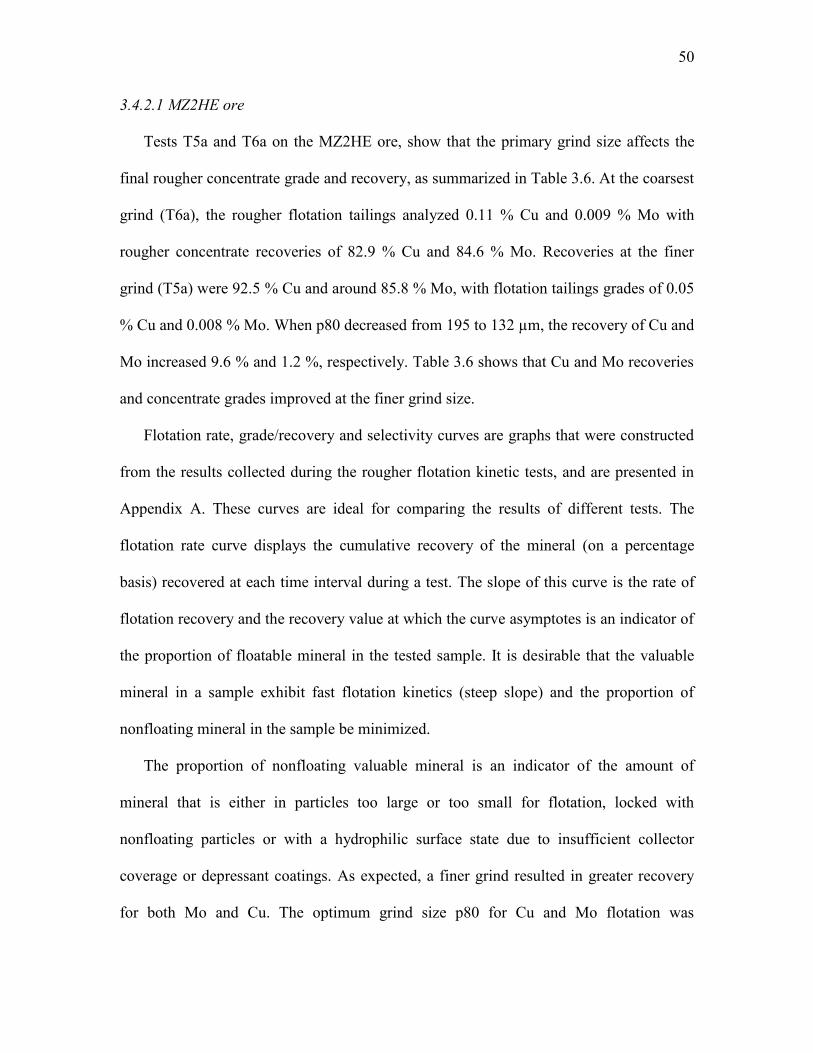
50
3.4.2.1 MZ2HE ore
Tests T5a and T6a on the MZ2HE ore, show that the primary grind size affects the
final rougher concentrate grade and recovery, as summarized in Table 3.6. At the coarsest
grind (T6a), the rougher flotation tailings analyzed 0.11 % Cu and 0.009 % Mo with
rougher concentrate recoveries of 82.9 % Cu and 84.6 % Mo. Recoveries at the finer
grind (T5a) were 92.5 % Cu and around 85.8 % Mo, with flotation tailings grades of 0.05
% Cu and 0.008 % Mo. When p80 decreased from 195 to 132 µm, the recovery of Cu and
Mo increased 9.6 % and 1.2 %, respectively. Table 3.6 shows that Cu and Mo recoveries
and concentrate grades improved at the finer grind size.
Flotation rate, grade/recovery and selectivity curves are graphs that were constructed
from the results collected during the rougher flotation kinetic tests, and are presented in
Appendix A. These curves are ideal for comparing the results of different tests. The
flotation rate curve displays the cumulative recovery of the mineral (on a percentage
basis) recovered at each time interval during a test. The slope of this curve is the rate of
flotation recovery and the recovery value at which the curve asymptotes is an indicator of
the proportion of floatable mineral in the tested sample. It is desirable that the valuable
mineral in a sample exhibit fast flotation kinetics (steep slope) and the proportion of
nonfloating mineral in the sample be minimized.
The proportion of nonfloating valuable mineral is an indicator of the amount of
mineral that is either in particles too large or too small for flotation, locked with
nonfloating particles or with a hydrophilic surface state due to insufficient collector
coverage or depressant coatings. As expected, a finer grind resulted in greater recovery
for both Mo and Cu. The optimum grind size p80 for Cu and Mo flotation was

51
approximately 132 µm. For MZ2HE, the rougher kinetic results for Cu and Mo recovery
are displayed in Figure 3.8. Furthermore, the slope and tendency of the flotation rate of
both fine and coarse grinding are quite similar, which indicates that there are no more
than one or two factors that account for their recovery. Results indicate that generally, the
Cu flotation rate for the fine grinding was much better than that for the coarse grinding.
The flotation rates were stabilized after 3 minutes in both cases. Particle morphology
such as size and liberation state could be the main issue affecting Cu loss for the MZ2HE
ore.
However, with Mo, there is no significant difference in Mo recovery between fine
and coarse grinding. It is difficult to speculate on the reason for the loss of Mo.
However, the nature of the lost particles have been examined using advanced
characterization instruments, and an explanation for the difference in the flotation
response is presented in Chapter 5. Also, separation efficiency of any concentration
operation can be expressed by a curve showing the recovery attainable for any value of
concentrate grade. The theoretical grade/recovery curve for an ore is a definition of the
maximum expected recovery by flotation of a mineral at a given grade. To establish the
theoretical grade/recovery curve for a mineral, a mineralogical liberation study should be
undertaken using tools such as QEMSCAN, MLA and HRXMT.
Using these tools in combination with standard flotation tests can quickly and
efficiently define the efficiency of a process and show where potential improvements
may be made. In the current research, the experimental grade/recovery curve obtained
from flotation kinetic data and chemical composition were created at each time interval.
This curve does not, however, give an estimate of the grade and recovery achievable in a

52
multiple stage flotation circuit. However, this curve does give a good relative measure of
selectivity. The experimental grade/recovery curves of the MZ2HE ore based on flotation
kinetic data when the p80 grind size was reduced from 195 µm to 132 µm are presented
in Figure 3.9. There exists an inverse relationship between concentrate grade and
cumulative recovery. If the concentrate grade is very high, it implies that it has minimal
contamination with gangue material and inevitably some of the valuable minerals lost to
the tailings and cumulative recovery will be low. Separation efficiency increases in the
direction defined by the arrow in Figure 3.9. Figure 3.9 shows cumulative grade/recovery
curves in which Cu and Mo were floated after coarse grinding (solid line) and then after
fine grinding (dashed line), to determine if grind fineness could give an improved
performance. Four sequential timed concentrates were taken in each case. The fine
grinding curves appear to show similar flotation initially, then the curves for Cu recovery
significantly increased, but the grade decreased slightly from 12.5 – 11.7 % with an
increase in fine grinding.
Therefore, with significant increase in Cu recovery, the grade was only slightly
compromised. It was expected that the additional Cu particles were directed into the
rougher concentrate after fine grinding. That is why these fully and/or partially liberated
Cu particles are increasing Cu recovery and decreasing Cu grade in the rougher
concentrate. In the case of Mo flotation, Mo recovery and grade showed no significant
differences in the MZ2HE ore. It was expected that liberation was not the reason for Mo
loss. If a comparison of size-by-size recovery analysis of Cu and Mo was made on both
feeds and rougher tailings, then we might be able to explain the reason for low Mo
recovery using HRXMT analysis.

53
3.4.2.2 LSE ore
Two different grind sizes were tested on the LSE ore sample to evaluate the effect of
the lithological characteristic on the flotation. Table 3.7 indicates that Cu and Mo
recoveries and grades improved significantly at the finer grind size.
The recoveries of Cu and Mo increased 9.34 % and 8.47 %, respectively, when the
p80 decreased from 220 µm to 148 µm. As expected, a finer grind resulted in greater
recovery for both Mo and Cu. The optimum grind size (p80) for Cu and Mo flotation
was at 148 µm. Furthermore, with both the fine and coarse grinds, the recovery kinetic
curves for the Cu and Mo, were quite similar, which indicates that there are no additional
factors that account for their recovery. For the LSE ore, kinetic results for Cu and Mo
recovery are shown in Figure 3.10. Results indicate that generally, flotation rates of Cu
and Mo continually increased in the coarse grinding stage. This increase was significantly
decreased after fine grinding.
It might be explained that these minerals were liberated from gangue minerals and
then easily floated after fine grinding but the kinetic curve for these minerals still did not
reach a plateau on the graph. This slight increase in Cu and Mo loss could be explained
by a different factor, which can affect flotation performance. The experimental
grade/recovery curves of the LSE ore are illustrated in Figure 3.11.
The grade/recovery curves can also give some additional information relating to
“slow” and “fast” floating effects of chalcopyrite and molybdenite. Fast floating effects
are mainly related to particle size and liberation (the difference between the 1st
concentrate at 0-1 minute) issues and slow floating is explained by surface oxidation and
slime coating effects. In the LSE ore, the Cu recovery increased from 79.1 % to 88.5 %,

54
as more Cu was liberated, but the grade had no significant difference with an increase in
grind fineness. Hence, we can expect that liberation does not affect grade and this
phenomenon may attribute to slime coating. Slime coating and slime aggregation could
be a dominant issue in the loss of Cu and Mo for the LSE ore.
In other words, as indicated in the graph for the grade/recovery curve of Cu, the slope
of the flotation rate curve for Cu minerals was less steep for the coarser ground material,
and then it increased during the fine grinding stage.
3.4.2.3 MZ2S ore
A similar series of tests was conducted on the MZ2S ore sample to confirm the
response of different mineralization materials to the grind size. Cu recovery increased
from 87.6 % to 91.2 % with decreasing particle grind size from p80 of 205 µm to 146
µm. Table 3.8 shows that Cu recovery and grade improved at the finer grind size but Mo
exhibited a reverse result and recovery and grade significantly decreased.
The losses of Mo were considerable at the grind size p80 of 146 µm. At the finest
grind (T3a), the final flotation tailings graded 0.11 % Cu and 0.019 % Mo with rougher
concentrate recoveries of 91.2 % Cu and 75.6 % Mo. As shown in Figure 3.12, Mo
recovery at the finer grind (T3a) was significantly lower than the flotation recoveries of
the other ore types. Compared with coarse grinding, the recovery of Cu in fine grinding
increased 3.6 % and recovery of Mo decreased 5.2 %. For the MZ2S ore, flotation
kinetic results for Cu and Mo recovery are presented in Figure 3.12.
Results indicate that the flotation rate of Cu and Mo continually increased for both
fine and coarse ground material. Their flotation rates did not stabilize and the froth

55
formation was very weak during the first 10 minute flotation period under standard
testing conditions.
With an increase in dosage of flotation reagent and time, the flotation performance (as
judged from froth formation) improved considerably, resulting in well mineralized, stable
and thick froth.
The grade/recovery curves of the MZ2S ore for Cu and Mo when the grind size was
reduced from p80 of 205 µm to 146 µm are shown in Figure 3.13. During first few
minutes of flotation, the Cu grade increased from 26.5 – 30.5 % and the whole curve was
pushed up to the right, presenting greater opportunities for recovery improvement to be
made. The increased recovery at the finer grind size can be seen to rise from 87.6 % to
91.3 % in the cumulative concentrate grade with 22.5 % Cu. It was expected that the
recovery of Cu is mainly dependent on the liberation state than on other factors of this ore
type because the new, freshly exposed surfaces of the Cu particles could actively contact
with the flotation reagent after fine grinding. However, Mo recovery was still
unpredictable and it is difficult to explain reason for the lost Mo particles. In the case of
Mo, all new surfaces are reacting with an unknown chemical compound or species.
To understand the general characteristics of the flotation response achieved with this
ore type, the rougher tailings samples were studied using optical microscopy. Upon visual
inspection, the molybdenum minerals were found to be round like a disk, smooth, and
clean in the rougher concentrate. Also, all the isolated Mo mineral particles appeared to
be well liberated. Significantly, similar molybdenite particles were observed in the MZ2S
rougher tailings. The photomicrograph for the MZ2S rougher tailing sample is presented
in Figure 3.14. The general mineralogical composition for the rougher tailings of the

56
MZ2S ore not only consisted of chalcopyrite, molybdenite, pyrite and quartz (gangue),
but also a significant amount of Fe oxide minerals, such as hematite and magnetite, were
regularly observed in this ore type. Also, the surface of the Mo particle seemed to be very
brittle, strongly damaged and sometimes coated by some white powdery minerals on its
surfaces and Mo loss was comparatively higher than for other ore types. This could be
explained by the fact that the MZ2S ore had undergone significant surface oxidation, but
visual inspection could not explain and confirm the reason for the loss of Mo.
The oxidation of near-surface sulfide minerals by atmospheric oxygen is critical for
understanding and determining the flotation environment of weathering of sulfide-
bearing bulk minerals. To better understand the reasons for such sulfide in the tailings,
further detailed characterization studies were carried out using SEM-EDS and XPS
analysis in order to understand why these naturally hydrophobic molybdenite particles
were lost in the tailings. It was expected that either gangue mineral slimes were adsorbing
onto the surface, or that surface oxidation and scale precipitation were occurring from the
process water. As reported by many researchers, water chemistry plays an important role
in molybdenite flotation due to the highly reactive edge surfaces of molybdenite crystals,
particularly for fine molybdenite particles with large edge-to-face ratio. However, the
appearance of sulfide minerals in the tailings is not normally expected.
3.5 Summary and discussion
In summary, 64 samples representing 7 ore types from Bingham Canyon were
evaluated with batch rougher flotation tests and several ore types have been identified as
difficult-to-float. The flotation recovery of Cu and Mo from these ore types is far inferior
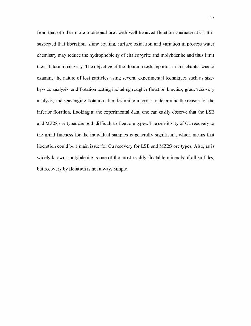
57
from that of other more traditional ores with well behaved flotation characteristics. It is
suspected that liberation, slime coating, surface oxidation and variation in process water
chemistry may reduce the hydrophobicity of chalcopyrite and molybdenite and thus limit
their flotation recovery. The objective of the flotation tests reported in this chapter was to
examine the nature of lost particles using several experimental techniques such as size-
by-size analysis, and flotation testing including rougher flotation kinetics, grade/recovery
analysis, and scavenging flotation after desliming in order to determine the reason for the
inferior flotation. Looking at the experimental data, one can easily observe that the LSE
and MZ2S ore types are both difficult-to-float ore types. The sensitivity of Cu recovery to
the grind fineness for the individual samples is generally significant, which means that
liberation could be a main issue for Cu recovery for LSE and MZ2S ore types. Also, as is
widely known, molybdenite is one of the most readily floatable minerals of all sulfides,
but recovery by flotation is not always simple.

58
Figure 3.1 Results of copper (a) and molybdenum (b) recovery of batch flotation tests for each ore type, at a grind target of 25% plus 100 mesh (modified from FLSmidth, 2012).
70
80
90
100
MZ2HW MZM1 RECDOME MZ1H MZ2HE LSE MZ2S
Cu
rec
ove
ry,
%
Ore type
50
60
70
80
90
100
MZ2HW MZM1 RECDOME MZ1H MZ2HE LSE MZ2S
Mo r
ecove
ry,
%
Ore type

59
Figu
re 3
.2
The
sche
mat
ic
flow
shee
t fo
r sa
mpl
e pr
epar
atio
n an
d su
bseq
uent
ch
arac
teriz
atio
n an
alys
is.

60
Figure 3.3 Laboratory rod mill used for grinding calibration tests prior to liberation and flotation testing.

61
Figure 3.4 Schematic diagram of the standard flotation test work including a detailed characterization analysis.
Grinding
Flotation experiment
Characterization analysis
Recommendation
Re-flotation experiment
Rougher
Rougher concentrate
Slime coating Surface oxidation Liberation Contaminant of process water
De-sliming Re-grinding Ultrasonic treatment
Concentrate Tailings
Second stage
First stage

62
Figure 3.5 Particle size distributions of the LSE (a) and MZ2S (b) ore samples after grinding for different times.

63
Figure 3.6 Grind calibration curve of the LSE, MZ2S and MZ2HE ore types.
R² = 0.9928
R² = 0.9784
R² = 0.9934
5
15
25
35
45
55
6 8 10 12 14 16 18 20
Th
e per
cen
tag
e of
plu
s 10
0 m
esh
, %
Grinding time, min
LSE ore type
Mz2S ore type
Mz2HE ore type

64
Figure 3.7 Cu and Mo recovery of the MZ2HE, LSE and MZ2S ore samples at different grind fineness.
70
80
90
100
LSE Mz2S Mz2HE
Cu
rec
ove
ry, %
Coarse grinding - 35 % + 100 meshFine grinding - 25 % + 100 mesh
60
80
100
LSE Mz2S Mz2HE
Mo
rec
ove
ry, %
Coarse grinding - 35 % + 100 meshFine grinding - 25 % + 100 mesh

65
Figure 3.8 MZ2HE ore: copper (red) and molybdenum (blue) flotation kinetics
during rougher flotation. Solid line represents coarse grinding at 35% +100 mesh and dashed line represents fine grinding at 25% -100 mesh.
0
20
40
60
80
100
0
20
40
60
80
100
0 2 4 6 8 10
Mo
ly r
eco
very
, %
Co
pp
er r
eco
very
, %
Flotation time, minute
Fine grinding - CuFine grinding - MoCoarse grinding - CuCoarse grinding - Mo
Increasing flotation rate
Increasing proportion of floatable minerals

66
Figure 3.9 Illustration of typical form of grade/recovery curves for froth flotation based on chemical analysis and rougher flotation kinetic data MZ2HE ore. Each curve represents the cumulative grade vs. the cumulative recovery for each time interval.
0.5
1.0
1.5
2.0
2.5
3.0
0
5
10
15
20
55 65 75 85 95
Cu
mu
lati
ve M
o g
rad
e, %
Cu
mu
lati
ve C
u g
rad
e, %
Cumulative recovery, % (Cu/Mo)
Fine grinding - CuCoarse grinding - CuFine grinding - MoCoarse grinding - Mo

67
Figure 3.10 LSE ore: copper (red) and molybdenum (blue) flotation kinetics during rougher flotation. Solid line represents coarse grinding at 35% +100 mesh and dashed line represents fine grinding at 25% + 100 mesh.
0
20
40
60
80
100
0
20
40
60
80
100
0 2 4 6 8 10
Mo
ly r
eco
very
, %
Co
pp
er r
eco
very
, %
Flotation time, minute
Fine grinding - CuFine grinding - MoCoarse grinding - CuCoarse grinding - Mo

68
Figure 3.11 Illustration of typical grade/recovery curves for froth flotation based on chemical analysis and rougher flotation kinetic data of the LSE ore.
0.5
1.0
1.5
2.0
2.5
3.0
5
10
15
20
25
30
35
45 55 65 75 85 95
Cu
mu
lati
ve M
o g
rad
e, %
Cu
mu
lati
ve C
u g
rad
e, %
Cumulative recovery, % (Cu/Mo)
Fine grinding - CuCoarse grinding - CuFine grinding - MoCoarse grinding - Mo
Fast floating
Slow floating

69
Figure 3.12 Flotation kinetics of the MZ2S ore showing the relation between the Cu and Mo recoveries with respect to the flotation time.
0
20
40
60
80
100
0
20
40
60
80
100
0 2 4 6 8 10
Mo
ly r
eco
very
, %
Co
pp
er r
eco
very
, %
Flotation time, minute
Fine grinding - CuFine grinding - MoCoarse grinding - CuCoarse grinding - Mo

70
Figure 3.13 Illustration of typical form of grade/recovery curves for the rougher flotation of the MZ2S ore.
0.5
1.0
1.5
2.0
2.5
3.0
5
10
15
20
25
30
35
25 35 45 55 65 75 85 95
Cu
mu
lati
ve M
o g
rad
e, %
Cu
mu
lati
ve C
u g
rad
e, %
Cumulative recovery, % (Cu/Mo)
Fine grinding - CuCoarse grinding - CuFine grinding - MoCoarse grinding - Mo

71
Figure 3.14 Lost sulfide particles in the rougher tailings of the MZ2S ore sample; photomicrograph by optical microscopy.
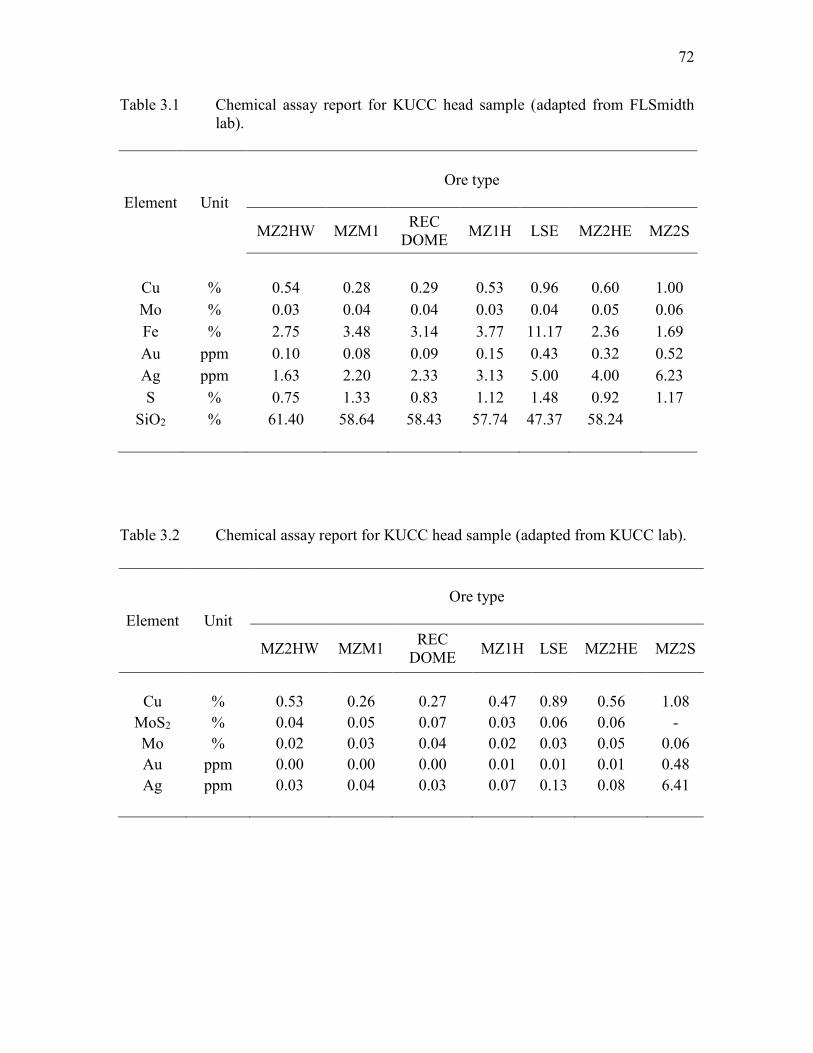
72
Table 3.1 Chemical assay report for KUCC head sample (adapted from FLSmidth lab).
Element Unit
Ore type
MZ2HW MZM1 REC DOME MZ1H LSE MZ2HE MZ2S
Cu % 0.54 0.28 0.29 0.53 0.96 0.60 1.00 Mo % 0.03 0.04 0.04 0.03 0.04 0.05 0.06 Fe % 2.75 3.48 3.14 3.77 11.17 2.36 1.69 Au ppm 0.10 0.08 0.09 0.15 0.43 0.32 0.52 Ag ppm 1.63 2.20 2.33 3.13 5.00 4.00 6.23 S % 0.75 1.33 0.83 1.12 1.48 0.92 1.17
SiO2 % 61.40 58.64 58.43 57.74 47.37 58.24
Table 3.2 Chemical assay report for KUCC head sample (adapted from KUCC lab).
Element Unit
Ore type
MZ2HW MZM1 REC DOME MZ1H LSE MZ2HE MZ2S
Cu % 0.53 0.26 0.27 0.47 0.89 0.56 1.08 MoS2 % 0.04 0.05 0.07 0.03 0.06 0.06 - Mo % 0.02 0.03 0.04 0.02 0.03 0.05 0.06 Au ppm 0.00 0.00 0.00 0.01 0.01 0.01 0.48 Ag ppm 0.03 0.04 0.03 0.07 0.13 0.08 6.41

73
Table 3.3 Designated reagent dosage in the flotation stage.
Units Cytec 8989 Burner oil F - 549
Density
g/cc
1.166
0.81
0.99
Purity % 65 100 100 Grind study test lb/t - 0.04 - Rougher kinetic test lb/t 0.035 0.07 0.046 Reflotation test lb/t 0.010 0.05 0.023
Table 3.4 Summary of experimental results of the grind calibration study for the LSE and MZ2S ore types.
Ore type LSE MZ2S
Grind time, minute 8 12 16 8 14 20
Ca(OH)2, gm
1.2
1.9
2.4
1.2
1.9
2.4
pH 9.8 9.6 10.48 9.8 9.4 10.32 % + 100 mesh 40.7 27.1 13.0 42.4 33.5 18.4
p80 266 182 120 303 206 144
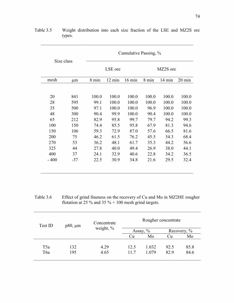
74
Table 3.5 Weight distribution into each size fraction of the LSE and MZ2S ore types.
Size class
Cumulative Passing, %
LSE ore
MZ2S ore
mesh µm 8 min 12 min 16 min 8 min 14 min 20 min
20 841 100.0 100.0 100.0 100.0 100.0 100.0 28 595 99.1 100.0 100.0 100.0 100.0 100.0 35 500 97.1 100.0 100.0 96.9 100.0 100.0 48 300 90.4 99.9 100.0 90.4 100.0 100.0 65 212 82.9 95.8 99.7 79.7 94.2 99.3
100 150 74.4 85.5 95.8 67.9 81.3 94.6 150 106 59.3 72.9 87.0 57.6 66.5 81.6 200 75 46.2 61.5 76.2 45.5 54.3 68.4 270 53 36.2 48.1 61.7 35.3 44.2 56.6 325 44 27.8 40.0 49.4 26.9 38.0 44.1 400 37 24.1 32.9 40.6 22.8 34.2 36.5
- 400 -37 22.5 30.9 34.8 21.6 29.5 32.4
Table 3.6 Effect of grind fineness on the recovery of Cu and Mo in MZ2HE rougher flotation at 25 % and 35 % + 100 mesh grind targets.
Test ID p80, µm Concentrate weight, %
Rougher concentrate
Assay, % Recovery, %
Cu Mo Cu Mo
T5a
132
4.29
12.5
1.032
92.5
85.8 T6a 195 4.65 11.7 1.079 82.9 84.6

75
Table 3.7 Effect of grind fineness on the recovery of Cu and Mo in the LSE rougher flotation at 25 % and 35 % + 100 mesh grind targets.
Test ID p80, µm Concentrate weight, %
Rougher concentrate
Assay, % Recovery, %
Cu Mo Cu Mo
T1a
148
4.17
20.2
0.678
88.5
82.5 T2a 220 4.11 18.2 0.554 79.1 74.0
Table 3.8 Effect of grind fineness on the recovery of Cu and Mo in the MZ2S rougher flotation at 25 % and 35 % + 100 mesh grind targets.
Test ID p80, µm Weight, %
Rougher concentrate
Assay, % Recovery, %
Cu Mo Cu Mo
T3a
146
4.42
22.5
0.922
91.2
75.6 T4a 205 4.15 21.1 1.064 87.6 80.8

76
CHAPTER 4
IDENTIFICATION OF TRACE MINERAL PARTICLES
IN FLOTATION TAILINGS USING RAPID SCAN
RADIOGRAPHY
4.1 Introduction
New processing technology for improved productivity and efficiency is the key to
success in today’s highly competitive market place. It has been well established that
appropriate analytical control systems can provide such improvements. This is especially
true of the particle separation processes used in the coal and mineral industries (Miller
and Lin, 1988, 2004, 2009, 2013; King and Schneider, 1993). As the technology
advances, the industry is always looking forward to a better technique for mineral
characterization. Most present methods rely on heavy liquid fractionation, or on
microscopy observation of a series of thin or polished sections (King and Schneider
1993) of the particulate sample. Optical microscopy is an invaluable tool for
mineralogical characterization of ores and rocks. The minerals are identified from their
optical properties. The optical properties differ from mineral to mineral because their
crystal structure is different, as well as the chemical constituents of the mineral; also,
their relative positions in the crystal lattice sites differ. However, it becomes difficult to

77
identify all minerals using only the optical microscope because there are cases where the
optical properties of one mineral very closely resemble another (King and Schneider,
1993; Sutherland, 1998; Das et al., 2008). In addition, the traditional examination
methods for multiphase mineral particles using 2D polished section images by optical
microscopy is extremely time consuming, labor intensive, and has many limitations,
including long sample preparation time, biased sampling, limited information, and
consistent overestimation of the extent of liberation (Miller and Lin, 2004, 2009).
Therefore, a nondestructive technology (NDT) method called XMT has been
developed for 3D mineral particle examination with the advantages of simple sample
preparation, shorter analysis time, and statistically reliable accuracy and confidence of
identification for multiphase minerals (Miller et al., 2009). As the resolution and the
techniques for 3D analysis have advanced in the last decade, it is now possible to map in
detail the microstructure and texture of multiphase particulate systems in 3D digital space
(Miller and Lin 2009; 2013).
For trace mineral components such as molybdenite, the content is in the range of parts
per million (ppm), which means that millions of particles must be examined to provide
statistically reliable accuracy and confidence in the characterization analysis. HRXMT
offers a quantitative imaging capability that can produce high resolution 3D images of the
internal structure of multiphase particulate samples at a resolution of several µm (Miller
and Lin, 2004, 2009) with a sample size of 1000x1000x1000 or about 1000 million
voxels (volume elements). Another issue is sample analysis time for characterization,
especially for trace mineral components. It should be noted that a full 3D tomography
scan usually takes about several hours to half of a day depending on the desired voxel

78
resolution, 5 to 1 µm, respectively. In the case of HRXMT, thousands of projections of
the sample may be needed, whereas in the case of radiography a projection of only a few
seconds is used for analysis.
In this research, rapid scan dual energy (DE) radiography including a calibration
procedure was used to evaluate and isolate trace mineral particles, such as chalcopyrite
and molybdenite in flotation tailings at the ppm level. Dual energy (DE) radiography is
the simplest and easiest option of multi-energy radiography. DE radiography involves
taking two radiographic images at both high and low energy levels, and using the results
of both scans to calculate the relative reflex and the effective atomic number, leading to
elemental analysis. Rapid scan DE radiography is time efficient, especially compared to
HRXMT. For example, more than 40,000 particles, 150x75 µm in size, can be
interrogated in less than 15 minutes and the composition of particles containing high-
density mineral phases estimated. After DE radiography scanning, these trace particles
can then be isolated for detailed analyses such as liberation/exposure analysis by
HRXMT and/or selected for surface characterization using XPS, ToF-SIMS, or other
analytical instruments. Rapid scan DE radiography can also be used for the examination
of drill core samples, tailings samples, or any other particulate sample containing trace
mineral particles. In this chapter, first, the procedure for calibration will be demonstrated
and then applications given to identify mineral particles using DE radiography.
This research provides an alternative way for mineral characterization using the DE
method of the X-ray system in order to reduce the experimental cost and lead time,
improve data accuracy, and data reliability. Mineral particles in monosize distribution can
be identified with the relative reflexes and thickness. Each radiographic image can be

79
acquired in a very short time and is able to analyze several million particles.
4.2 Basic principles of DE radiography
4.2.1 Background and basic theory
Details about the theory and the principles of general radiography are available in
many textbooks such as Martensen (2010) and Kahn and Gaskin (2012). Use of DE
radiography was described early in the 1970s for medical applications (Alvarez and
Macovski, 1976; Brody et al., 1981; Cardinal and Fenster, 1990). Later in 2002,
consideration of applications in the mineral industry was reported (Schena et al., 2002,
2003). Reviews of the theory of DE radiography for material characterization are briefly
summarized in the literature (Heaven et al., 2010; Schena et al., 2003). Several patents
described a DE X-ray method imaging the fast moving material on a conveyer belt and
using these images to calculate the grade of the stream (UK patent GB 2083618, 1982;
US patent 6122343, 2000). X-ray radiography can be used to produce a 2D map of X-ray
attenuation coefficients of irradiated ore samples. The intensity of the X-ray traveling
through a mineral particle is attenuated (McCullough, 1975). As demonstrated in Figure
4.1 (a), a monochromatic X-ray of energy, 𝐸, and incident intensity (number of
photons/unit time and area), 𝐼0, on passing through local material, that absorbs X-ray
photons and having a thickness, 𝑥, will have a transmitted intensity, 𝐼, given by:
𝐼 = 𝐼0 ∙ 𝑒𝑥𝑝 (−𝜇(𝜌 , 𝑍, 𝐸) ∙ 𝑥)
where 𝜇 is the linear attenuation coefficient, depending on density, 𝜌, atomic number, 𝑍
(3)

80
and the energy of the X-ray beam, 𝐸.
By taking the logarithm of the ratio of incident and transmitted intensity, Equation 3
can be rearranged as:
ln (𝐼 𝐼0⁄ ) = −μ(𝜌 , 𝑍, 𝐸) ∙ 𝑥
As mentioned before, depending on the sample density, atomic number, thickness and
the X-ray energy, the attenuation coefficient of the material can be determined as (Van
Geet et al., 2001):
𝜇 = 𝜌(𝑎 + 𝑏𝑍3.8 𝐸3.2⁄ )
where 𝜌 is the bulk density, 𝑍 is the effective atomic number of the material, 𝐸 is the
X-ray energy, 𝑎 and 𝑏 are constants, which are energy dependent. As shown in Figure 4.1
(b), the log transmission through two minerals, A and B, is the sum of the log
transmission of each mineral:
ln (𝐼 𝐼0⁄ ) = −𝜇𝐴( 𝐸) ∙ 𝑥𝐴 − 𝜇𝐵( 𝐸) ∙ 𝑥𝐵
Equation 6 consists of two unknowns (𝑥𝐴 and 𝑥𝐵), which can be solved from
radiography measurements at two energy levels (low and high).
ln (𝐼𝐿 𝐼0L⁄ ) = −𝜇𝐴(𝐸𝐿) ∙ 𝑥𝐴 − 𝜇𝐵(𝐸𝐿) ∙ 𝑥𝐵
(4)
(5)
(6)
(7)

81
ln (𝐼𝐻 𝐼0H⁄ ) = −𝜇𝐴(𝐸𝐻) ∙ 𝑥𝐴 − 𝜇𝐵(𝐸𝐻) ∙ 𝑥𝐵
Then, the unknown thicknesses (𝑥𝐴 and 𝑥𝐵) can be solved as:
𝑥𝐴 = (𝜇𝐵(𝐸𝐻) ∙ 𝐿𝐴𝐿 − 𝜇𝐵(𝐸𝐿) ∙ 𝐿𝐴𝐻) ∆⁄
𝑥𝐵 = (−𝜇𝐴(𝐸𝐻) ∙ 𝐿𝐴𝐿 + 𝜇𝐴(𝐸𝐿) ∙ 𝐿𝐴𝐻) ∆⁄
where ∆, 𝐿𝐴𝐿 and 𝐿𝐴𝐻 are :
∆= 𝜇𝐴(𝐸𝐿)𝜇𝐵(𝐸𝐻) − 𝜇𝐴(𝐸𝐻)𝜇𝐵(𝐸𝐿)
𝐿𝐴𝐿 = ln(𝐼0𝐿(𝐸𝐿) 𝐼𝐿(𝐸𝐿)⁄ ) and 𝐿𝐴𝐻 = ln(𝐼0𝐻(𝐸𝐻) 𝐼𝐻(𝐸𝐻)⁄ )
The log of the attenuations, 𝐿𝐴𝐿 and 𝐿𝐴𝐻, are measured at each pixel for both the low-
energy and high-energy radiographic images.
Basically, two methods were used to identify and isolate mineral particles from
gangue minerals based on the radiography theory. Method 1 involved the calculation of
the effective atomic number of minerals based on the relative reflexes between two
energy radiographies and its corresponding main sample. Method 2 involved the
estimation of relative thickness and was used, as a calibration standard to evaluate
accuracy in the prediction of the thickness of high and low density minerals and its
corresponding audit sample. Method 1 is more practical, but method 2 can provide a
more accurate assessment of analytic variability.
(8)
(9)

82
4.2.2 Calculation of effective atomic number
Initially, the effective atomic number can be estimated based on the relative reflex
from DE radiography. For two energy levels (low and high), Equation 3 can be written
as:
𝐼(𝐸𝑖) = 𝐼0(𝐸𝑖)∙ 𝑒𝑥𝑝(−𝜇(𝜌 , 𝑍, 𝐸𝑖) ∙ 𝑥); 𝑖 = 𝐿𝑜𝑤, 𝐻𝑖𝑔ℎ
Differentiation of mineral phases within the sample is complicated because the linear
attenuation coefficient, 𝜇, at each voxel depends directly on the electron density, the
effective atomic number, 𝑍𝑒𝑓𝑓, of the material comprising the sample, and the energy of
the X-ray beam, 𝐸. A simplified equation that illustrates the approximate relationship
among these quantities is a general form of Equation 5:
𝜇(𝐸𝑖) = 𝜌[𝛼(𝐸𝑖) + 𝛽(𝐸𝑖) ∙ 𝑍𝑝]
where the functions 𝛼(𝐸𝑖) and 𝛽(𝐸𝑖) define the energy dependence of Compton and
photoelectric effects, respectively. For the mineral system in this study, the p is set as 3.8.
The effective atomic number is simplified, as 𝑍𝑒𝑓𝑓 ≡ 𝑍 and the radiography reflex is
defined as:
𝑅(𝐸𝑖) = 𝑅𝑖 = ln(𝐼0,𝑖 𝐼0⁄ )
at a specific energy level, 𝐸. Then, Equations 11 and 12 can be combined as:
(12)
(10)
(11)

83
𝑅(𝐸𝑖) (𝜌 ∙ 𝑥⁄ ) = 𝜇𝑚 = [𝛼𝑖 + 𝛽𝑖 ∙ 𝑍𝑝] ∙ 𝑍)
where 𝜇𝑚 =𝜇
𝜌⁄ is the mass attenuation coefficient. Based on the operating energy range
(40 kV to 150 kV for the DE radiography), the DE radiography technique involves both
the Compton and photoelectric effects with p ≈ 3.8 for this study. Three known
materials and measurements in a specific energy range using the DE radiographic
technique (Naydenov et al., 2003) can calculate the effective atomic number of an
unknown material. In this case, the relative reflex of two radiographs, 𝑋 = 𝑅1 𝑅2⁄ plays
the principal role in the estimation of the effective atomic number, 𝑍𝑒𝑓𝑓, of an unknown
material. From Equation (12),
X≡ 𝑅(𝐸1) 𝑅(𝐸2)⁄ = 𝜇𝑚(𝐸1) 𝜇𝑚(𝐸2)⁄ = 𝜇(𝐸1) 𝜇(𝐸2)⁄
Therefore, X depends only on the effective atomic number and does not depend on
the geometry (thickness, x) or the density (𝜌) of the material nor does it depend on its
other physicochemical properties.
In this way, the 𝑍𝑒𝑓𝑓 of an unknown material can be estimated based on DE
radiography.
𝑍𝑒𝑓𝑓 = ((𝑘1 ∙ 𝑋 + 𝑘2) (𝑘3 ∙ 𝑋 + 𝑘4)⁄ )1
𝑝⁄
where 𝑋 = 𝑅1 𝑅2⁄ is the relative reflex from two radiographs at different energy levels
(high and low), and the calibration coefficients 𝑘1, 𝑘2, 𝑘3 and 𝑘4 are determined from the
(13)
(14)
(15)

84
relative reflexes of three known materials as described by the following equations.
𝑘1 = 𝑍1𝑝 ∙ 𝑍2
𝑝 ∙ (𝑋1 − 𝑋2) − 𝑍1𝑝 ∙ 𝑍3
𝑝 ∙ (𝑋1 − 𝑋3) + 𝑍2𝑝 ∙ 𝑍3
𝑝 ∙ (𝑋2 − 𝑋3)
𝑘2 = 𝑋1 ∙ 𝑋2 ∙ 𝑍3𝑝 ∙ (𝑍1
𝑝 − 𝑍2𝑝) − 𝑋1 ∙ 𝑋3 ∙ 𝑍2
𝑝 ∙ (𝑍1𝑝 − 𝑍3
𝑝)+𝑋2 ∙ 𝑋3 ∙ 𝑍1𝑝 ∙ (𝑍2
𝑝 − 𝑍3𝑝)
𝑘3 = 𝑋1 ∙ (𝑍1𝑝 − 𝑍2
𝑝) − 𝑋2 ∙ (𝑍1𝑝 − 𝑍3
𝑝) + 𝑋3 ∙ (𝑍1𝑝 − 𝑍2
𝑝)
𝑘4 = 𝑋1 ∙ 𝑋2 ∙ (𝑍1𝑝 − 𝑍2
𝑝) − 𝑋1 ∙ 𝑋3 ∙ (𝑍1𝑝 − 𝑍3
𝑝) + 𝑋2 ∙ 𝑋3 ∙ (𝑍2𝑝 − 𝑍3
𝑝)
where 𝑋1, 𝑋2 and 𝑋3 are the relative reflexes of three known materials using the DE
method; 𝑍1, 𝑍2 and 𝑍3 are their effective atomic numbers, and p is set as 3.8. The
calibration constants depend upon the chosen energy values used in the radiation source,
characteristics of the detector, etc., but not upon properties of the material. These
constants are determined from a series of test measurements using objects of known
composition and geometry.
Generally, this method provides the capability to calculate the effective atomic
number of unknown minerals using the DE method. The DE method works well as long
as the energy range for each measured element does not involve the K-edge effect. With
the effective atomic number and mineralogy of the sample, the unknown material can be
characterized.
4.2.3 Estimation of effective thickness (relative composition)
Heaven’s work (Heaven et al., 2010) reported a thickness calculation based on the
dual energy method and two known materials using the following transformation. To
characterize the gangue minerals (silicate) and trace mineral component (high density,
(16)

85
high Z) using the DE radiographic technique, aluminum (Al) and copper (Cu) were
chosen as materials A and B, due to their similarity to the attenuation coefficients for
gangue (quartz) and high density trace minerals (chalcopyrite, molybdenite), as shown in
Figure 4.2. Polychromatic X-ray sources provide X-ray photons with a distribution of
energy levels and the photon absorption needs to be solved with a nonlinear function for
the log attenuation values.
As shown by Cardinal and Fenster (1990), the approximate solution for a
polychromatic X-ray source, a simplified equation that illustrates the approximate
relationship for unknown thickness (𝑥𝐴 and 𝑥𝐵), can be solved as:
HdLdHcLHcLcHcLccx
HbLbHaLHaLaHaLaax
B
A
10
254
23210
10
254
23210
1
1
where 𝑥𝐴 and 𝑥𝐵 are the thicknesses of A and B for each pixel in the reconstructed
images for the two known materials, respectively. The 16 unknown coefficients
𝑎0…5, 𝑏0,1, 𝑐1…5, and 𝑑0,1 can be estimated from calibration of low- and high-
energy radiographic images with a combination of 5 known thickness levels for both
materials, A and B.
(17)

86
4.3 Materials and methods
4.3.1 DE radiography
The high-resolution X-ray micro computed tomography (HRXMT) system at the
University of Utah has been the main instrument used to acquire DE X-ray radiographs.
Major external and internal components of the Xradia MicroXCT-400 machine are
shown in Figure 4.3 and Figure 4.4, respectively. Based on a polychromatic focal X-ray
source, the scan conditions have been considered and optimized in order to obtain high
quality images. As the most important consideration of the DE method, the source energy
is set at 80 kV for the low-energy level, which is satisfactory for Cu mineral scans, and at
140 kV for the high-energy level, which is mostly for high density minerals such as
galena and gold. The lens magnification was set at 4X, providing an image resolution of
around 5 µm per pixel, and a field of view approximately 5 mm by 5 mm.
This magnification meets the need for particle size classes from 1 mm to 50 µm; a
physical 150 µm thick glass filter is used to remove the noise caused by low energy X-
ray photons, and to improve the contrast of silicate minerals. In order to have an
appropriate field of view, the distances between the sample to source and sample to
detector, are set at 20 millimeters and 44 millimeters, respectively. The effect of scattered
radiation is excluded.
The exposure time is set at 5 seconds per radiograph to obtain sufficient X-ray photon
counts for the sample. Binning is set at 2 for a moderate exposure time and image quality,
which goes to 1024 pixels on the X and Y axes. Finally, the image for measurement is an
average of 10 radiographs.
Both sample sets were compressed to 1 millimeter thickness by plastic plates

87
(76.2x25.4x1.0 mm) from both sides, and stabilized by double-sided tape on one side of
the plastic slide. The slides and tape helped keep the sample fixed on the sample stage
while absorbing only a small amount of X-ray photons, which were resolved by
references.
4.3.2 Sample preparation and standard calibration
Two sets of samples were prepared for calibration of DE measurements. The first
sample set was assembled of six different minerals. This sample set was measured by
three known materials to calculate an unknown material effective atomic number
following Naydenov’s work (Naydenov et al., 2003). Aluminum and Cu foils comprised
the second sample set following Heaven’s work (Heaven et al., 2010).
4.3.3 Experimental procedure
Rapid scan DE radiography was used to locate the high and medium density minerals
with a series of radiographic images taken at both a high- and low-energy levels in a very
short time.
A step-by-step experimental procedure of rapid scan DE radiography is included in
Appendix C. In order to obtain a quick and accurate evaluation by radiographic analysis,
monosize particle distribution must be organized for sample preparation. These
conditions not only help identify specific mineral phases by quick radiographic
evaluation, but reduce misinterpretation caused by the transmission distance, similar
minerals, or particle size.
If the attenuation coefficient of the objective mineral is much higher than that of the

88
host minerals, it will be much easier to identify and locate a specific mineral. To enhance
the image contrast, the distance of the source/detector, exposure time and physical filters
should be considered to establish a high quality radiograph.
4.4 Results and discussion
4.4.1 Determination of unknown coefficients
The DE radiographic procedure allows for calibration specific to minerals of interest
with improved discrimination and accuracy. In addition, the DE technique requires that
data be collected at two energies sufficiently different to define primary contributions
from photoelectric interactions and Compton scattering.
To determine the unknown coefficients 𝑎0…5, 𝑏0,1, 𝑐0…5 and 𝑑0,1 of Equation 16, DE
pairs from radiographs for an Al step-wedge and a Cu step-wedge standard, or reference,
were used for calibration. In this regard, the Al foil and Cu foil are stacked as interlaced
layers, as shown in Figure 4.5 (a). Each Cu foil has a thickness of 35 µm, and each Al foil
has a thickness of 110 µm. In this way, 5 Cu foil samples and 5 Al foil samples were
combined and glued on the plastic plates. A total of 36 sections were measured with each
section being approximately a 0.3mm x 0.3mm square area. Radiographs of the Al and
Cu wedges stacked for DE calibration at 80 kV and 140 kV are shown as Figures 4.5 (b)
and 4.5 (c), respectively.
Averaged radiographic images for reference materials were taken following the same
scan conditions specified in Section 4.3.1 using the absorption mode. The Al foil samples
of increasing thickness were stacked from left to right (alphabetic sequence from A to F)
and Cu foil samples of increasing thickness were stacked from top to bottom (numeric

89
sequence from 1 to 6).
The log transmission results as well as the actual thickness of the Al and Cu for each
rectangle were input into a Microsoft Excel spreadsheet. The unknown coefficients can
be determined using a minimization solver (Brown, 2001). Once values of corresponding
coefficients have been determined, the calculated thicknesses of Cu and Al foils can be
determined using Equation 16. In this study, the generalized reduced gradient method
built into Excel’s solver tool (Brown, 2001) was used to fit the data from Table 4.1. The
measured thickness of these Al and Cu wedge steps are listed in the top row and the left
column of Table 4.1. The measurements of the log attenuation values corresponding to
the sections of Al and Cu wedges acquired from radiographic analysis at DE levels of 80
kV (white column) and 140 kV (gray shaded column) are listed in Table 4.1. ImageJ
software (National Institutes of Health: http://rsbweb.nih.gov/ij/) was used to measure
relative intensities of the radiographic images. To minimize registration errors with the
wedges, the horizontal and vertical edges of the wedges were used as fiduciary
landmarks; the top and bottom of the wedge steps are parallel. The step outlines were
made with ImageJ well away from the edges of the steps. Low (L)- and high (H)– energy
images of the stacked wedges were used for calculation of the coefficients for Equation
16.
The measured mean pixel values in a region of interest in both high and low energy
images from each of the 25 rectangles were used to convert to the negative log of the
energy transmission,−𝑙𝑛(𝐼𝑟𝑒𝑐𝑡𝑎𝑛𝑔𝑙𝑒 𝐼𝑎𝑖𝑟⁄ ) values, to obtain the data in Figure 4.5. The
actual thicknesses of the wedges were measured 3 times with a Duratool electronic
micrometer. As presented in Table 4.2, after 10 iterations, values of corresponding

90
coefficients 𝑎0…5, 𝑏0,1, 𝑐0…5 and 𝑑0,1 for Equation 16 were determined. The spreadsheet
calculations adjusted the unknown coefficients iteratively to determine the coefficients
that produced the best fit between the actual thicknesses and the calculated thicknesses.
The calibration data and the corresponding coefficients are only valid for the imaging
parameters reported in this work. Changes of the kV, X-ray generator, sensor, source-to-
detector distance, or the calibration wedges would necessitate obtaining new calibration
images, collection of data, and calculation of new coefficients. To determine the accuracy
of the coefficients, 25 calculated thicknesses were compared to the measured thicknesses
with the corresponding standard deviation, as shown in Figure 4.6, from section A1 to
E5.
Similarly, 25 reconstructed measurements are plotted for each Cu step-wedge. It is
noted that a highly significant correlation is found between the measured step-wedge
thickness and the calculated thickness from DE radiography for the Cu wedge.
Furthermore, a prediction of Al and Cu wedge thicknesses for sections A6 and F6 are
also calculated and presented in Table 4.3. However, a larger spread in Al thickness for
each step is observed from the result of Table 4.3. It is expected that the noise is higher
for the calculated Al foil thickness (low density material) than for the Cu foil thickness
(high density material) (Gauntt and Barnes, 1994). The standard deviations of each
section are less than 3 %. The coefficients are acceptable for the level of accuracy
desired.
Second, samples consisting of six different materials (quartz, aluminum, copper,
molybdenite, gold and lead) were prepared for the determination of effective atomic
numbers using DE radiography measurements. The positions of the calibration materials

91
(quartz, aluminum, copper, molybdenite, gold, and lead) and related DE radiographs
acquired at 80 and 140 kV are shown in Figure 4.7.
In this case, aluminum, copper and lead were selected as known materials. These
three elements can represent the three different mineral phases usually present in samples
from metal mining operations having low attenuation coefficients (gangue,
quartz/silicates), medium attenuation coefficients (copper, most base metal minerals) and
high attenuation coefficients (molybdenite, galena, lead or other precious metals). Quartz,
molybdenite and gold were selected as the unknown materials for validation. Although
the plastic plates and double-sided tape absorb some X-ray photons, this does not matter
since the ratio is taken and the absorption contribution is the same for each mineral
sample. Material information used for the determination of effective atomic numbers
based on DE radiography is listed in Table 4.4. Samples were arranged in a 5mm x 5mm
area and 4X magnification used for each single projection (radiograph), without moving
the sample or the source/detector. Coefficients 𝑘1, 𝑘2, 𝑘3, and 𝑘4 were then calculated
according to Equation 15 using 𝑝 = 3.8. Yielding, 𝑘1 = 1.37 ∙ 1012, 𝑘2 = −1.20 ∙
1012 , 𝑘3 = −1.15 ∙ 106 and 𝑘4 = 6.57 ∙ 105.
The calculated effective atomic number was then compared to the real effective
atomic number to determine the accuracy in data correlation. Figure 4.8 shows the
estimated and actual effective atomic numbers based on the relative reflex of the two
radiographs, X. Since the polychromatic maximum energy for this instrument is about
150 kV and 10 watts flux, these settings could be insufficient for the reflex to determine
the high effective atomic number for materials such as gold. In this regard, instrument
capability could limit identification to material with an effective atomic number less than

92
40. Also, the impurity of gold could affect the experimental result. A universal
dependence has been predicted for the effective atomic number as a function of relative
radiographic reflex. The established theoretical law is nearly confirmed by the
experimental data presented.
4.4.2 Applications of rapid scan DE radiography
A very important part of using rapid scan DE radiography is the creation of an
accurate and complete mineral reference library (MRL) that is used to classify the
minerals in a sample or sample suite. The MRL is made up of mineral names or mineral
attenuation coefficient groupings associated with the relative reflex of two energy level
(low and high) radiographies. To evaluate the feasibility and accuracy of identification
for a rapid search and isolation of the lost mineral particles in flotation tailings, 9
different mineral particles with 150x75 µm size, which were separated from the KUC ore
sample, were spread on the double sticky tape on the plastic plates. Results are shown in
Figure 4.9 (a) and the DE radiograph acquired from the indicated region as shown by
Figure 4.9 (b).
Minerals listed in Table 4.5 are the most abundant minerals of the copper porphyry
ore samples from the Bingham Canyon mine, KUC, and confirmed and isolated by the
Geological Department at the University of Utah from pure minerals. The actual effective
atomic numbers of the reference minerals were calculated by a standard equation (Taylor
et al., 2009) and their densities can found at http://www.mindat.org/ (Ralph and Chau,
1993). Preliminary results indicate the mineral particles with high effective atomic
numbers, 𝑍𝑒𝑓𝑓, are identified very well as shown in Figure 4.9. Using the same scan

93
conditions and the same coefficients obtained in Section 4.4.1, these nine pure minerals
were scanned to verify the accuracy of the coefficients K1, K2, K3 and K4. As shown in
Figure 4.9 (b), the dark grey area represents minerals with high density/high atomic
numbers, the midgrey areas represent the medium density/medium atomic number
minerals, and the light grey areas indicate the surrounding background and low atomic
number minerals. In most cases, the region of interest (ROI) of the mineral could contain
different materials with different transmission values. Porosity (air or water) and
impurities of the selected mineral (molybdenite containing a talc inclusion), for example,
may affect calculation of the mean relative reflex value.
Specially, one needs to consider the partial volume effect (PVE) of the ROI on the
radiography image and all these effects should be removed before statistical analysis. If
particles are surrounded by background, PVE definitely occurs, as shown in Figure 4.10.
If this is the case, a ROI of a mineral can be manually drawn, and the mean value of
counts in that region can be calculated for determination of the mean pixel value. The
method to correct or consider the impurity and porosity of a mineral is to determine the
confidence interval of the intensity value. A confidence interval gives an estimated range
of intensity values that is likely to include an unknown population parameter, the
estimated range being calculated from a given set of sample data. The formula for the
confidence interval (CI) of the mean of the relative reflex as presented in the Equation 18.
𝐶𝐼 = 𝑠𝑎𝑚𝑝𝑙𝑒 𝑠𝑡𝑎𝑡𝑖𝑠𝑡𝑖𝑐 ± 𝑚𝑎𝑟𝑔𝑖𝑛 𝑜𝑓 𝑒𝑟𝑟𝑜𝑟 = �̅� ± 𝑍(𝑆 √𝑛⁄ )
In this formula, �̅� is the mean of the intensity data; 𝑍 is the interval coefficient, which
(18)

94
can be found from the normal distribution table (for example, the interval coefficient for
a 95% confidence level is 𝑍 = 1.96), 𝑆 is the standard deviation of the data and 𝑛 is the
pixel numbers. The margin of error (± 𝑍𝑆
√𝑛 ) of a confidence interval is defined to be the
value added or subtracted from the sample mean which determines the length of the
interval.
In this particular case, 9 different minerals with their specific relative reflexes have
been determined. The confidence intervals for each mineral can be calculated separately,
as shown in Figure 4.11. Bubble charts are popular tools for identifying and illustrating
measurement clusters. Essentially, these bubble charts allow four different variables to be
plotted within the same graph, making it easy to assess the relative statistical
performance. For example, each mineral circle, identified by color and size, is plotted on
the chart based on the relative reflex (x-axis) and the effective atomic number (y-axis).
The size of the circle represents the confidence interval of intensity values of the relative
reflex for each mineral.
As shown on Figure 4.11, some bubbles such as chalcopyrite and sphalerite are
overlapping. Using this method, it is easy to differentiate elements with a large difference
between their effective atomic numbers; for example, it is easy to tell the difference
between quartz (Zeff = 11.8) and molybdenite (Zeff = 36.4). However, for minerals with
closer atomic numbers, such as chalcopyrite (Zeff = 25.0), azurite (Zeff~24.5) and
sphalerite (Zeff = 25.4), it is impossible to differentiate them using DE radiography. Of
course, there is another way to improve accuracy of radiographic inspection. Further,
multi-energy approaches (3 or 4 energy levels) may be capable of discriminating these
minerals.

95
The estimated effective atomic numbers used the coefficients K1, K2, K3 and K4,
which were determined from standard calibration with 𝑝 = 3.8. These are then compared
to the actual effective atomic numbers to determine the accuracy in data correlation, as
shown in Figure 4.12. Figure 4.12 shows how close the estimated effective atomic
numbers based on the relative reflex of the two radiographs, X, were to their actual
effective atomic numbers. The standard deviations of the values of effective atomic
numbers are less than 10 %. The coefficients were acceptable for the level of accuracy
needed to locate and identify desired particles. However, a wider spread of effective
atomic numbers of high density and high attenuation coefficient minerals was observed in
Figure 4.12.
It is noted that the maximum energy of the X-ray system was not enough for the
relative reflex to determine high effective atomic number materials such as galena and
barite. It is expected that DE radiography uses X-rays to determine the attenuation
coefficients; but it is very dependent on the ability of the X-rays to penetrate the sample.
This means that for higher density minerals, the machine in use may not be able to
produce X-rays with a high enough energy to go completely through the sample.
Therefore, this further limits which minerals can be identified using DE radiography.
Such reference minerals rarely occur in the KUC flotation tailings.
General mineralogical characterization of the Cu rougher tailings revealed that apart
from the gangue minerals, the main sulfide minerals are chalcopyrite, pyrite and
molybdenite. Some amount of covellite and iron oxide minerals such as hematite were
also present. A histograms of the relative reflex of these common minerals in the KUC
rougher tailings is presented in Figure 4.13. Data were analyzed and displayed in a
96
histogram (a column chart that displays frequency data) by using the histogram tool of
Minitab 16 software (Minitab, 2011).
To create a histogram, the radiography data were organized in two columns that
contain input data and frequency or bin numbers on the worksheet. Input data are the data
of relative reflexes of each mineral to be analyzed. Molybdenite particles selected for
calibration analysis based on optical microscopy appeared to be completely liberated,
smooth and pure. However, as seen from Figure 4.13, there was an unusual overlapping
between the relative reflex values of molybdenite and bornite, causing suspicion that this
could be due to inaccuracy in identifying the molybdenite particle. The particle was
further carefully examined by SEM analysis, which revealed the presence of some
silicates and pores. Hence, it is understood that porosity and impurity impacts the X-ray
intensity values of the selected minerals. This phenomenon is also observed in oxidized
minerals like malachite and hematite. The results of this investigation are summarized as
follows:
1. Based on the relative reflex of MRL data, all minerals in the flotation products
can be grouped into three main categories (high, medium, and low) by effective
atomic numbers and attenuation coefficients.
2. High and medium attenuation coefficient minerals (molybdenite and chalcopyrite)
can be easily differentiated from gangue minerals based on the relative reflex of
two radiographs.
3. The basic weakness of the DE radiography method is that it is difficult to
differentiate minerals with similar effective atomic numbers such as chalcopyrite
and sphalerite or pyrite and iron oxide, leading to errors in the elemental analysis

97
and particle identification, as exemplified in Figure 4.13.
4. The accuracy of mineral identification was found to be at 𝑍𝑒𝑓𝑓 ≥ 26 ± 6 for high
and medium density minerals depending upon many variables such as
characteristics of the X-ray source (non-monochromatic), statistical and other
fluctuations, including poor energy resolution, noise, scattered radiation and
porosity or impurity of material.
To verify and to further evaluate the feasibility of the rapid search and isolation of
trace mineral particles, a sample with 150x75 µm particle size from flotation tailings was
prepared and several molybdenite particles of the same size placed at known positions
within this sample. DE radiographs were acquired from 40 (4x10) adjacent regions and
show stitched images of different locations. The stitched images were composed of a
total of 40 – 50 images per one slide. The projection region for each radiograph image is
25 mm2 containing about 450 - 500 particles and the total projection time for a single DE
radiographic image and the reference image took 15 seconds. In addition, a reference
image was taken at both low and high energies for every slide so that a correct reference
could be applied for every slide. As stated in Section 4.2.2, the reference image
normalizes the attenuation coefficients to a percentage of the transmission. This
essentially makes the difference between the attenuation coefficients larger, increasing
the contrast in the image. Figure 4.14 illustrates the identified molybdenite particles
found in the center image of the bottom images in Figure 4.14 (b). Then, identified
molybdenite particles were confirmed by optical microscopy, as shown in Figure 4.14
(c). Several particles containing Cu sulfide mineral with a lower effective atomic
number than molybdenite were placed in the sample slide. Each radiographic image can

98
be acquired in a very short time and is able to analyze several millions of particles per
day. In addition, for identification of Cu sulfides in drill core samples without the detailed
analyses of association and liberation, DE radiography was applied. Results indicate that
larger cores up to 25 mm can be imaged, but smaller samples were the focus in this
situation. Cubic Cu ore particles (3x3x3 mm) were prepared and DE radiographs were
acquired, as shown in Figure 4.15. As shown in Figure 4.15, results indicate that Cu
sulfides are identified with a reconstructed thickness of less than 0.2 mm inside the 3 mm
thickness cubes. The gray scale indicates thickness from 0 mm (black) to 0.256 mm
(white). It is also noted, as expected, the reconstructed thickness of the rock block is
slightly higher than the actual thickness (3 mm). From such measurements, the volume
percent of the sulfide minerals for the three cubic Cu ore particles (3x3x3 mm) can be
determined, as shown at the bottom of Figure 4.16.
HRXMT is a nondestructive technique that has the capability to generate 3D images
of particulate beds. In this regard, to further evaluate the accuracy using DE radiography,
these three cubic Cu ore particles were scanned by HRXMT. In practice, when raw data
collected from HRXMT analysis were processed to generate 3D reconstruction of the
sample, the attenuation coefficient values in each voxel were translated to scaled CT
number values. Scaled CT number values are used in the classification process for
identification of the different minerals. More detailed information about the scaled CT
number and identification of minerals is presented in Chapter 5.
Generally, the HRXMT equipment is calibrated using standard pure Cu mineral
samples (Miller and Lin, 2013). A scaled CT number range is assigned to each pure
mineral. In this way, the identification of the different mineral phases is accomplished in

99
the scanned samples according to the scaled CT number values. Comparison of the
radiographs and 3D tomography images from a similar viewing angle is shown in Figure
4.17. For volume rendering of 3D images, sulfide mineral grains were set as a brown
color, pink was set for mineral phases with attenuation coefficients higher than
chalcopyrite and the gangue phase was set as a semitransparent green color. The
estimation of the composition in volume percent from a 3D tomography image is
included in the bottom row for comparison. As expected, the estimate from DE
radiography is underestimated due to the use of the Cu calibration wedge, which has a
higher X-ray attenuation coefficient than most of the Cu minerals. Based on 3D
tomography analysis of the samples, the proposed DE radiography technique was indeed
faster and more time efficient than only X-ray tomography or QEMSCAN analysis and
the potential additional data that could be gathered made this technique worth exploring for
future projects, especially if it involves identification of trace particles concentrated on a
small, parts per million scale. DE radiography provides some limited but important key
information by shooting just two radiographic images in a few seconds, while a detailed
examination such as HRXMT and QEMSCAN, usually takes a few hours to a day.
In other words, based on sampling statistics during DE radiography inspection, huge
amounts of detailed data significantly increase the possibility of finding the desired particles
(molybdenite) in low concentration products such as flotation feed and tailings.
Secondly, the scan is a 2D image of all sample particles, providing the spatial location of
a specific region or selected particle. The noninvasive, nondestructive sample preparation and
scan procedure allow the desired minerals to remain in the sample for further analysis.
Thirdly, sample preparation and prescan time is easy and short. In this regard, rapid scan DE
radiography can recognize the region of the sample containing the targeted mineral phase

100
first, then a complete characterization analysis such as HRXMT, SEM-EDS, and XPS
analysis can be implemented to characterize the specific mineral phases, as shown in Figure
4.18. Finally, the technique was demonstrated for fast geometallurgical analysis such as
identification of heavy metal minerals, specifically Cu and Mo sulfides, and an estimate
of their amount in run-of-mine ore and trace heavy metal particles in flotation tailings. In
the future, the DE method will be able to integrate the rapid-radiography scan for a
complete examination procedure before the HRXMT scan as a more accurate choice.
4.4.3 Identification of lost minerals in KUC rougher tailings
4.4.3.1 Data acquisition and file conversion
As previously mentioned in Section 3.3.4, approximately 3 - 5 g of representative
sample portions were obtained using a rotary sample divider from rougher tailings, and
spread over plastic plates for preparation of a sample suitable for rapid scan DE
radiography examination. A total of 120 slides of rougher tailings samples of three
different Cu ore types (MZ2S, LSE, and MZ2HE) from KUC ore for the whole project
have been prepared and considered for identification and isolation of lost sulfide
minerals, such as molybdenite and chalcopyrite, using this method. In other words, each
ore type was compared in two categories of grind fineness (coarse and fine) and
examined for two coarse size classes (50x100 mesh, 100x200 mesh) from each grind
fineness. Ten slides were prepared from each size class. Several examples of the resulting
scans are shown in Figure 4.19.
The DE radiography scans are completed by splitting the slide into 40 sections,
making a 4x10 grid, and scanning each section at a low-energy level (80 kV) and a high-

101
energy level (140 kV). These were scanned using the averaging mode on the Xradia
MicroXCT-400 machine, taking 3 images at 5 seconds each to average together and
produce a single image. Generally, all rougher tailings samples were scanned under the
same conditions using rapid scan DE radiography. The scan conditions were set at the
following: 4X magnification with 5 seconds exposure time; source voltages at 80 kV and
140 kV; the distance between source and detector -44 mm and 20mm; the detector
binning at 2 with a 150 µm glass filter.
The Xradia MicroXCT-400 at the University of Utah provides applications called
XMController and XMReconstructor (Xradia, 2010) for image acquisition and
reconstruction. Radiographic images in 2D for both high- and low-energy levels were
acquired using an averaging mode and visualized by XMController on the screen, and
then saved as a radiography file pattern with extension .xrm. The XRM file contains
information of X-ray intensity, coordinates, exposure time, source voltages, distances,
etc. In addition to the internal image format (.xrm) from Xradia, several image formats
can be exported, namely, tiff, jpeg, and raw.
According to the specifications of the MicroXCT-400, the maximum color depth of
the CCD detector is 16-bit grayscale and radiography scans are saved in a grayscale,
unsigned 16-bit (xrm) file. In the present study, it would be a time consuming process to
export 80 radiographic images (both at high- and low-energy levels) using the
XMController without losing original image data. It usually takes more than 20 minutes
for each slide. In this regard, instrument capability limited conversion of radiographic
images in a short time. After the DE radiography scans were completed, file conversion
time from .xrm file to .bin file could be reduced approximately 200 times using the

102
corresponding Mathlab code, as shown in Appendix B. The binary file .bin format is the
same format as the .raw file with simply a different extension. When all files were
converted into .bin and/or .raw file, the calculation of the relative reflex was easily
performed using Matlab software (Mathworks, 2012), according to Equations 11 and 13.
Once digital radiography images with .xrm file extensions were converted into 8-bit,
grayscale, .raw files, which contain basic experimental values based on the pixel
intensities of the relative reflexes, then the effective atomic numbers of each mineral
could easily be calculated. In addition, the labeling of each file could contain some
additional information. Having the assistance of the file name, the ore type, grind
fineness, size class, number of slide, types of flotation products (concentrate, tailings and
feed) and the corresponding location of lost particles on the slide could be defined. For
example, a name of any radiographic image contains the following information:
LSE_oretype_finegrinding_plus100mesh_slide_1_roughertail_Section1x1.xrm
In Figure 4.19, note the darker particles in each radiography scan, these could be
potential molybdenite minerals. Based on chemical analysis, the estimated numbers of
lost chalcopyrite and molybdenite particles in KUC flotation tailings are presented in
Table 4.6.
As previously stated, each slide consists of 40 radiographic image sections. Based on
results of image analysis, one section contains approximately 450 – 500 particles. Each
slide contains roughly 18,000 – 22,000 particles in the 300x150 µm size class, so a total
of 220,000- 250,000 particles from each size class for each ore type could be imaged and
analyzed using the radiographic method.
The average analysis time for each slide was approximately 15 minutes. Depending

103
on the Mo content in the rougher tailings, the number of slides scanned from each size
classes was determined. If the Mo content was less than 0.003 %, approximately 10 slides
were acquired. This enabled the characterization and classification of these mineral
particles to be investigated. Therefore, an image-processing program was necessary to
analyze the lost minerals in the flotation tailings, as presented in Section 4.4.3.2.
4.4.3.2 Image processing and data analysis
Image processing and data analysis are the next important steps after image
acquisition and file conversion, because they allow for significant enhancement of the
visibility of the details in the digital radiographs. The entire process is semiautomatic and
high throughput. The automated determination of high atomic number minerals also
eliminates some elements of operator error. There are several image processing software
packages available such as ImageJ (Rasband, 1997), MIPAV (2007), and MATLAB
(2012), some commercial and some open-source.
Once the relative reflex, described in Section 4.2.2, was found from the low- and
high-energy scans using the appropriate Matlab code, it was saved as high resolution
radiographic images with extension .raw. After importing them into ImageJ, a Threshold
function was applied to these radiographic images. In general, good threshold can be
selected if the histogram peak of the desired mineral is tall, narrow, symmetric, and
separated by deep valleys. Commonly, flotation tailings are multiphase, heterogeneous
materials consisting of several different minerals. In the multiphase case, such as in this
research, a hysteresis (two levels) threshold, based on the pixel intensity histogram, is
applied for phase segmentation. As mentioned previously, thresholding removes

104
unwanted background information, leaving behind only the desired particles themselves.
Figure 4.20 shows the ImageJ tresholding function that segments the background from
molybdenite. The dialog box, Figure 4.20 (a), was opened after the tresholding function
was selected from the ImageJ menu bar. This histogram represents the distribution of
pixel intensities of relative reflex in 2D; pixels above the high threshold are classified as
molybdenite and below the low threshold as background. The lower and upper
thresholding (sliders) were selected from the calibration results presented in Figure 4.12.
In this case, all pixels between 0.74 and 0.82 represent medium/low density and
medium/low atomic number minerals and the pixel intensities below 0.74 represent high
density and high atomic number minerals in the sample. Using these tresholding values,
the radiographic image, Figure 4.20 (b), was segmented into features of interest
(molybdenite) and background (air and other minerals such as quartz, chalcopyrite and
pyrite). While adjusting, the threshold molybdenite particles are displayed in red and the
background is displayed in grayscale, Figure 4.20 (c). Once the thresholding function was
applied to the radiographic image, the background became white, leaving only the black
images of the desired particles, Figure 4.20 (d). Tresholding is not the final step for DE
radiography. Based on the relative reflex of thresholded particles, the effective atomic
number can be estimated for mineral identification.
Once all minerals with a high/medium density and a high/medium atomic number in
the rougher tailings have been found in the radiography images, lost molybdenite and
chalcopyrite particles can be located easily on the etched grid pattern. Isolation of desired
particles from the slide was manually done using microtweezers or high precision cutting
tweezers (TDI 14AGW-C) under simple optical microscopy. The microtweezers were the

105
best tool for picking up objects too small to be easily handled with the human hand. All
lost particles isolated from the rougher tailings were collected into the cylindrical aligned
container, subsequently undergoing further detailed analysis. Liberation analysis using
HRXMT was performed initially.
In conclusion, a schematic diagram of the DE radiography method is illustrated in
Figure 4.21 and the standard operating procedure broadly described in Appendix C.
Generally, the samples to be analyzed are initially split into narrow size fractions, each
size fraction distributed on projection plates, and the plates placed in the sample holder of
the MicroXCT-400 for irradiation at two energy levels (DE analysis). A single projection
image in 2D is captured by the detector, visualized on the screen according to the same
scan conditions as a standard sample and then saved as a radiography file pattern with
extension .xrm.
After completing the acquisition process at high- and low-energy levels, the averaged
reference is established. The reference should be prepared for both high- and low-energy
levels because each sample should have their own reference to remove X-ray attenuation
of the background, air and any other effects associated with the lens in order to enhance
image quality. All radiographic images are saved in the .xrm file after applying the
reference. Based on a combination of these two images, the relative reflex of X-ray
intensity can be calculated according to Equation 13, saved into a single radiographic file
and then converted from .xrm to .bin using the Matlab software for image data analysis.
As mentioned previously, one radiographic image is a relatively small image with 5x5
mm size but it contains 400 - 500 particles and analysis of this image requires
considerable processing time. This method can find the desired particles in a very short

106
time by subtracting the background and/or unnecessary gangue particles using
thresholding from the radiographic image.
In this research, this subtraction allows for isolatation of high density and high atomic
number minerals such as molybdenite from other minerals. The thresholded image is
used to calculate the effective atomic numbers of the particles for mineral identification.
4.4.3.3 Advantages and limitations of DE radiography
As mentioned before, radiography is one of the most important and widely used
methods in nondestructive technology. Each radiographic testing method offers a number
of advantages but each also has some limitations. A summary of advantages and
disadvantages of rapid scan DE radiography is outlined in Table 4.7.
One of the important benefits of DE radiography scanning is consumption of
considerably less disc space (4 megabytes/one image) than tomography. Use of less disc
space helps save storage space and also allows low-end computers to process the image
file under the system limitations.
4.5 Summary and discussions
The purpose of this work was to find an accurate, rapid, simple and easy method to
locate lost valuable mineral particles from rougher tailings samples of three KUC ore
types through their relative reflex of X-ray intensities using rapid scan DE radiography.
All of the findings in this work are based on the analysis of several mineral particles
covering a limited range of characteristics (particle size, effective atomic number, X-ray
intensity and X-ray attenuation coefficient). Accordingly, the conclusions from these

107
findings might apply only to these types of samples.
The findings serve as a model and as an initial study. As with any research, the initial
efforts define a starting point. Further work on other samples can then be considered in
reference to these data and the findings can then be either generalized or more
definitively qualified. A total of 160 slides were scanned by this method using the X-ray
system. The theory and procedures are described for the evaluation and isolation of trace
mineral particles from samples at the ppm level. In this regard, Al and Cu wedges were
used as calibration standards to evaluate accuracy in the prediction of the thickness of
high- and low-density minerals. In addition, the effective atomic number was determined
based on the relative reflex from DE radiography. The results demonstrate the feasibility
of DE radiography to identify mineral particles having a medium to high effective atomic
number (Zeff > 26), which is recommended for the identification and the isolation of trace
mineral particles. Then, these trace particles can be isolated for detailed characterization
analysis by HRXMT and/or selected for surface characterization using XPS, TOF/SIMS,
or other analytical instruments. The DE measurements correlated well with micron
measurement data taken for the Al and Cu wedges. In addition, it was concluded that the
dual energy approach allows one to improve the inspection efficiency by an order of
magnitude, in contrast to single energy methods.
The technique was demonstrated for rapid geometallurgical analysis and it was
expected that several millions of particles per day can be interrogated using this proposed
radiography method with an accuracy of up to 90%. Also, these developments can find
application not only in rapid geometallurgical analysis (identification of heavy metal
minerals, specifically Cu and Mo sulfides, and an estimate of their amount in run-of mine
108
ore and trace heavy metal particles in tailings), but also in areas such as identification of
mineral zones from drill core samples, mineral resource evaluation, mine planning and
the evaluation of separation efficiency of feed, tailings streams or any other particulate
sample containing trace mineral particles. Preliminary results verify that DE radiography
works well to fulfill this function.
The DE method is not optimal for quantification, but useful for sample
characterization into groups. Only the HRXMT scan or some other characterization
instruments can accurately describe the detailed mineral information. Nevertheless, the
dual energy method is truly helpful for examining the lost minerals in a short time, with
mass samplings, rather than doing full HRXMT scans. This reduces the experimental cost
and lead time, improves data accuracy, data reliability and improves their performance.
In the future, the rapid scan DE method should be able to integrate the rapid radiography
scan for a complete examination procedure before the HRXMT scan as a faster and more
accurate choice, and it could help to solve problems for difficult-to-float ores.

109
a) Single
b) Multiple
Figure 4.1 A simplified X-ray beam, 𝐼0 attenuated through single (a) or multiple (b) materials, having thicknesses, 𝑥A , 𝑥𝐵 results in attenuated beam, 𝐼.
Figure 4.2 Mass attenuation coefficients of Al and Cu representing the gangue mineral (quartz) and high density trace minerals (chalcopyrite and molybdenite) using a software application called XMuDat (Nowotny, 1998).
𝜇(𝐸) 𝐼0 𝐼
𝑥
𝜇𝐴(𝐸) 𝐼0 𝐼
𝑥𝐴
𝜇𝐵(𝐸)
𝑥𝐵
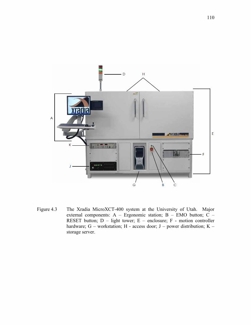
110
Figure 4.3 The Xradia MicroXCT-400 system at the University of Utah. Major external components: A – Ergonomic station; B – EMO button; C – RESET button; D – light tower; E – enclosure; F - motion controller hardware; G – workstation; H - access door; J – power distribution; K – storage server.

111
Figure 4.4 Visual internal view of the MicroXCT-400, with the access doors open. (A – Safety lock; B – X-ray source; C – Sample stage; D – visual light camera; E – detector assembly; F – turret; G – macrolenses).
B A
C
D
E
G F

112
Figure 4.5 Photo of stacked Al and Cu foils (a) and radiographs of the stacked Al and Cu wedges for DE calibration at 80 kV (b) and 140 kV (c).
Figure 4.6 Comparison between the measured step-wedge thickness and the reconstructed thickness from DE radiography for the Al foil and Cu foil wedges.
a) b) c)

113
.
Figure 4.7 DE radiographs (80 kV and 140 kV) of the quartz, aluminum, copper, molybdenite, gold and lead samples for determination of the unknown coefficient and effective atomic numbers. a) Low-energy level; b) high-energy level.
Figure 4.8 Estimated (line) and measured (points) data of effective atomic numbers based on the DE relative reflex of two radiographs, X.
a) b)

114
Figure 4.9 Microphotograph (a) and radiographic (b) image of main minerals (the detailed information is in Table 4.5) in Cu-Mo flotation tailings for DE calibration at 80 kV and 140 kV. 1 – molybdenite; 2 – galena; 3 – bornite; 4 – chalcopyrite; 5 – azurite; 6 – pyrite; 7 – hematite; 8 – sphalerite; 9 – quartz.
Figure 4.10 Partial volume effect dilutes the X-ray intensity values of a mineral during radiography analysis. In the case of MoS2, the resulting attenuated value is close to that of copper minerals, making it difficult to distinguish MoS2 from the other medium density and/or atomic number minerals.
1
2
3
4
5
6
7
8
9
a) b) a) b)

115
Figure 4.11 Dependence of the effective atomic number upon radiography reflexes in the regions of the photo effect and Compton scattering. The experimental dependence for materials of known composition are indicated.
Figure 4.12 Calibration curve for given 𝐾𝑖 and p-3.8 values and comparison between estimated (blue) and actual (red) effective atomic numbers from DE radiographs for each mineral.
BaSO4
MoS2 Cu5FeS4
(Zn, Fe)S2
Cu2CO3(OH)2
CuFeS2
Fe2O3
FeS2
SiO2
14
20
26
32
38
44
0.62 0.67 0.72 0.77 0.82 0.87
Th
e es
tim
ate
d e
ffec
tive
ato
mic
nu
mb
er,
Zef
f
Relative reflex, X
BaSO4
MoS2
Cu5FeS4
(Zn, Fe)S2
Cu2CO3(OH)2
CuFeS2
Fe2O3
FeS2
SiO2
PbS2
=∓ ∙ /√
PbS2
BaSO4
Cu5FeS4
MoS2
FeS2ZnS2
CuFeS2
Fe2O3
SiO2
Cu
Pb
Al
10
20
30
40
50
60
70
80
90
0.56 0.58 0.60 0.62 0.64 0.66 0.68 0.70 0.72 0.74 0.76 0.78 0.80 0.82 0.84 0.86 0.88
Th
e ef
fect
ive
ato
mic
nu
mb
ers,
Zef
f
Relative reflex, X
Estimated Zeff
Actual Zeff
Pure element standard
Poly. (Estimated Zeff)

116
Figure 4.13 Histogram of the relative reflex of the most common sulfide minerals in the KUC flotation tailings.
high medium low

117
Figu
re 4
.14
Mol
ybde
nite
and
cha
lcop
yrite
par
ticle
s id
entif
ied
for
each
sec
tion
of s
lide
base
d on
DE
radi
ogra
phy
and
optic
al in
spec
tion
for t
he se
arch
and
isol
atio
n of
trac
e m
iner
al p
artic
les.

118
Figure 4.15 Photo of cubic Cu ore particles (a) and the corresponding DE radiographs (b).
Figure 4.16 Sulfide mineral grains are identified from the estimated Cu minerals using DE radiography. Most of these mineral grains are less than 0.2 mm. a) radiography image; b) tomography image.
a) b)
a)
b)

119
Figure 4.17 Comparison of the cubic Cu ore particles (3x3x3 mm) using DE radiography (a) based on Figure 4.15 and 3D tomography (b) images, respectively.
.
Figure 4.18 Combination of DE radiography and detailed characterization analysis for mineral properties.
Feed,
Tailings, Drill core
DE
Radiography
HRXMT, XRD, XPS, SEM-EDS, TOF-SIMS, QEMSCAN
Mineral composition, Mineral liberation, Mineral exposure, Internal structure,
Particle size, shape.
Sample Isolation &
Identification
Detailed
characteristic
s
Final
results
a)
b)

120
a) Size class - 150 x 300 µm
b) Size class - 75 x 150 µm
Figure 4.19 DE radiography scans from the LSE rougher tailings (fine grinding – 25 % + 100 mesh size class). a) Coarse size class; b) medium size class. The images on the right are low-energy (80kV), and the images on the left are high-energy (140kV).
Low energy - 80 kV High energy - 140 kV
Low energy - 80 kV High energy - 140 kV

121
Figure 4.20 ImageJ thresholding function that segments the background and medium/low atomic number minerals from high atomic number minerals. a) Threshold dialog box; b) image of molybdenite particles prior to tresholding; c) threshold adjustment to match particles; d) final binary threshold image showing black particles on white background.
a) b)
c) d)

122
Figu
re 4
.21
Sum
mar
y of
rap
id s
can
dual
ene
rgy
(DE)
rad
iogr
aphy
and
its
appl
icat
ion
in t
he
anal
ysis
of t
ailin
gs sl
ides
.

123
Table 4.1 Measurement of log attenuation values from different sections of Al and Cu wedge steps (different thickness and composition) at 80 kV (white column) and 140 kV (gray shaded column).
Foil thickness, mm
A B C D E F
Aluminum foil
0.00 0.11 0.22 0.33 0.44 0.55 1
Copper foil
0.000 0.0 0.0 2.8 1.6 5.2 3.2 7.5 4.7 9.7 6.1 12.1 7.8 2 0.035 13.2 8.2 15.0 9.5 16.4 10.6 18.0 11.9 19.5 13.1 21.1 14.4 3 0.070 21.8 14.5 23.2 15.6 24.3 16.6 25.6 17.7 26.8 18.8 28.0 19.8 4 0.105 28.2 19.7 29.4 20.7 30.4 21.7 31.5 22.7 32.5 23.6 33.3 24.4 5 0.140 33.0 24.0 34.2 25.0 35.1 25.9 36.0 26.8 36.8 27.6 37.5 28.4 6 0.175 36.9 27.7 37.9 28.6 38.8 29.4 39.5 30.3 40.3 31.0 40.9 31.8
Table 4.2 Corresponding unknown coefficients used in Equation 16 for thickness estimation of Al and Cu foil wedges.
Reconstruction coefficients
for thickness of Al
Reconstruction coefficients for thickness of Cu
𝑎0 0.02 𝑐0 0.00 𝑎1 -0.84 𝑐1 28.15 𝑎2 1.49 𝑐2 -16.35 𝑎3 -0.01 𝑐3 0.18 𝑎4 0.01 𝑐4 -1.01 𝑎5 -0.01 𝑐5 0.41 𝑏0 -0.07 𝑑0 -4.00 𝑏1 0.04 𝑑1 -35.45

124
Table 4.3 Measured and calculated thicknesses of Al and Cu samples for sections A6 and F6.
Sections Transmission Thickness, mm Thickness, mm
L, 80 kV
H, 140 kV Al Al calc. Cu Cu calc.
A6 36.93 27.68 0.00 0.30 0.18 0.15 F6 12.07 7.81 0.55 0.53 0.00 0.01
Table 4.4 Measured log attenuation values and relative reflex, X, acquired from DE radiography used for the determination of effective atomic numbers for various materials.
Material Chemical formula
Effective
atomic number, Zeff
Log attenuation value
Relative reflex, X
80 kV 140 kV
Aluminum Al 13.00 74.62 85.42 0.87
Quartz SiO2 11.85 74.11 85.05 0.87 Copper Cu 29.00 63.00 78.05 0.81
Molybdenite MoS2 36.37 63.59 77.94 0.81 Gold Au 79.00 43.12 59.64 0.72 Lead Pb 82.00 16.74 28.31 0.59

125
Table 4.5 Basic properties of most abundant minerals of copper porphyry ore for dual energy radiography calibration.
Mineral
Effective atomic number, Zeff Density, g/cm3
Name
Formula
1 Molybdenite MoS2 36.37 4.62-4.73 2 Galena PbS2 75.21 7.31-7.58 3 Bornite Cu5FeS4 26.58 5.06-5.09 4 Chalcopyrite CuFeS2 25.00 4.10-4.30 5 Azurite Cu3 (CO3)2(OH)2 24.54 3.77-3.83 6 Pyrite FeS2 21.64 4.80-5.10 7 Hematite Fe2O3 22.69 5.10-5.25 8 Sphalerite (Zn, Fe)S2 25.40 3.90-4.20 9 Quartz SiO2 11.85 2.65-2.70
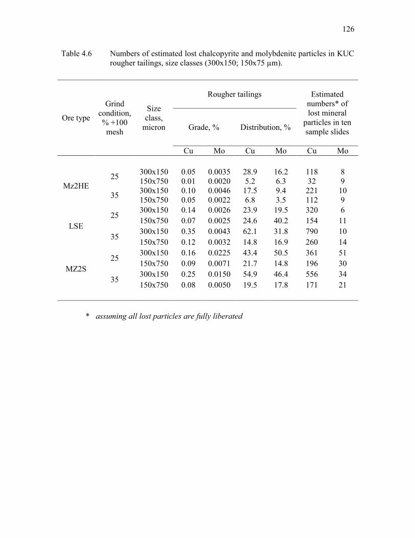
126
Table 4.6 Numbers of estimated lost chalcopyrite and molybdenite particles in KUC rougher tailings, size classes (300x150; 150x75 µm).
Ore type
Grind condition, % +100
mesh
Size class,
micron
Rougher tailings
Estimated
numbers* of lost mineral
particles in ten sample slides
Grade, % Distribution, %
Cu Mo Cu Mo Cu Mo
Mz2HE 25 300x150 0.05 0.0035 28.9 16.2 118 8
150x750 0.01 0.0020 5.2 6.3 32 9
35 300x150 0.10 0.0046 17.5 9.4 221 10 150x750 0.05 0.0022 6.8 3.5 112 9
LSE 25 300x150 0.14 0.0026 23.9 19.5 320 6
150x750 0.07 0.0025 24.6 40.2 154 11
35 300x150 0.35 0.0043 62.1 31.8 790 10 150x750 0.12 0.0032 14.8 16.9 260 14
MZ2S 25 300x150 0.16 0.0225 43.4 50.5 361 51
150x750 0.09 0.0071 21.7 14.8 196 30
35 300x150 0.25 0.0150 54.9 46.4 556 34 150x750 0.08 0.0050 19.5 17.8 171 21
* assuming all lost particles are fully liberated

127
Table 4.7 Summary of advantages and disadvantages of DE radiography method.
Advantages
Disadvantages
Major
Replaces tedious manual analysis
by systematic, computer automated analysis
Has difficulty
distinguishing minerals with very similar composition
Reduces the potential for operator bias and human error
Accuracy and precision of results is not high enough
Increases throughput and the number of mineral grains
examined, providing a more statistically representative
analysis of a sample
High degree of skill and experience is required for
exposure and interpretation
Has the ability to distinguish fine-grained or complexly
intergrown minerals at the scale of micrometer
The equipment is relatively expensive (especially for X-
ray sources)
Minor
Can detect both surface and
internal structure
Requires monosize
distribution
Significant variation of material can be detected by this method
Sample preparation is easy
Scanning time is short

128
CHAPTER 5
CHARACTERIZATION OF LOST PARTICLES IN
FLOTATION TAILINGS USING ADVANCED
INSTRUMENTATION
5.1 Introduction
Tailings evaluation can define the actual losses in a mineral processing plant, while
simultaneously defining why the losses occur and what might be done to flotation
efficiency. Of course, working with tailings is never easy. Minor or trace concentrations
of valuable minerals means that sample collection and integrity become a major concern.
Trace mineral analysis for minerals such as molybdenite is challenging and often the
process of selecting and preparing an appropriate, representative sample is more work
than undertaking the characterization analysis. Fast and accurate identification of lost
minerals in flotation products, such as feed and tailings, is a very important topic in
metallurgical engineering. Most particle identification methods often overlook and
miscount the trace mineral concentration in flotation tailings. To correct this, it is
proposed that the DE radiography method be used to quantitatively identify and collect
trace particles. Combining DE rapid scan radiography with other detailed characterization
methods may facilitate an accurate accounting of trace minerals at the parts per million

129
concentration, as described in Chapter 4. HRXMT, SEM and QEMSCAN can be used for
more accurate mineral identification and liberation analysis, once the lost mineral
particles are isolated from the tailings.
The objective of this phase of the dissertation research is to characterize the identified
and isolated valuable sulfide mineral particles from the rougher tailings and determine
their liberation state, association with other minerals and surface chemistry features. To
identify, characterize and quantify these lost particles, there are a variety of methods
available. The more traditional methods include elemental analysis done by XRF,
mineralogical analysis by XRD, mineral phase liberation analysis using automated SEM
techniques such as QEMSCAN or MLA, and HRXMT. Surface chemistry features can be
determined using XPS and ToF-SIMS.
5.2 Materials and methods
Generally, particulate materials are sampled from input (feed) and output products
(rougher concentrate and rougher tailings) of flotation and analyzed to evaluate the
efficiency of the separation. Specifically, rougher tailings from fine grinding experiments
were considered for detailed characterization analysis. The instruments used in this
section are optical microscopy, SEM, X-ray CT and XPS, whose operational details and
experimental methodology for characterization analysis are described in following
sections. The detailed analysis can be divided into four main categories:
Initial characterization analysis
Particle size distribution and size-by-size chemical analysis
Mineralogical analysis and liberation state analysis using SEM and HRXMT

130
Surface characterization analysis such as slime coating and surface oxidation
using SEM-EDS and XPS.
A schematic diagram of the procedure adopted to isolate and collect lost sulfide
mineral particles and the detailed characterization analysis is presented in Figure 5.1. In
the following Sections, 5.2.1, 5.2.2, and 5.2.3, instruments and methodology are
described.
5.2.1 Particle size distribution and size-by-size analysis
The purpose of size-by-size distribution analysis is to determine the Cu and Mo
distribution in the flotation products. After rougher flotation, representative portions
(approximately 150 grams) of samples of the flotation feed and tailings were split and
then screened into 5 size fractions by wet or dry screening using analytical screens with
quadratic openings. Five size classes were used to represent very coarse (>300 µm),
coarse (300x150 µm), medium (150x75 µm), fine (75x37 µm) and slime (<37 µm) size
fractions.
Initially, all samples were deslimed by wet screening at 400 mesh (37 µm). The
coarse fraction above 37 µm was dried, weighed and screened using standard sieves; 48,
100, 150, and 200 mesh and the certain amounts of samples were prepared for chemical
analysis. Each size fraction was assayed to determine copper, molybdenum and iron
content. Then, all molybdenite particles in each size class were collected and isolated
using the DE radiography method. The principle and experimental procedures of DE
radiography are well described in Chapter 4.

131
5.2.2 Liberation analysis using HRXMT
The micro tomography technique offers a unique capability for the quantitative
analysis of multiphase systems through the acquisition of high-resolution 3D images. One
important area of application for HRXMT is mineral liberation and mineral exposure
analysis (Miller and Lin, 1987; Gu and Napier-Munn, 1997; Lin and Miller, 2001; Videla
et al, 2007; Al-Wakeel et al, 2009). The X-ray micro tomography technique is able to
distinguish different mineral phases contained in ore particles based on the corresponding
computed tomography (CT) numbers for each phase. Lin and Miller (1996) described the
CT numbers for several of the most abundant copper minerals in copper porphyry ores
and the results are presented in Figure 5.2.
As a result of DE radiography inspection, lost sulfide particles were isolated from
rougher tailings samples and then all collected particles were poured into a plastic
cylinder of up to 4 mm in diameter. The sized samples do not require any other special
preparation. However, the sample needs to be well confined and held by frictional forces
because any small movement will cause reconstruction failure and error.
The sample was placed on the rotating stage between the X-ray source and the
detector, where photons pass through the sample and the projected image is captured by
the detector. Usually, a full tomographic 3D scan on the MicroXCT-400 requires 1000
projections and then the data are used to reconstruct the experimental data for liberation
analysis.
During tomography data acquisition, the scan conditions are an important issue in
order to obtain the best image quality. Image quality depends on many factors such as
source voltage, magnifications, distance between source and detector, physical filters,

132
field of view, exposure time, projection count and reference states (Xradia, 2010; Hsieh,
2012). As described by Lin and Miller (1996), an appropriate scan condition for image
acquisition of copper samples is presented in Table 5.1.
As mentioned before, the Xradia MicroXCT-400 provides an application called
XMController and XMReconstructor (Xradia, 2010) for image acquisition and
reconstruction. According to the specifications of the MicroXCT-400, the maximum
color depth of the CCD detector is a 16-bit grayscale, which means the CT reading is
between 0 and 65535 for each voxel. Initially, the results of an HRXMT scan were saved
in a grayscale, unsigned 16-bit tomography file using XMReconstructor. Then, the
tomography file was converted from a 16-bit unsigned short to an 8-bit unsigned byte
using MIPAV (McAuliffe, 2012). CT readings higher than molybdenite values can easily
be excluded by MIPAV software while file conversion is being completed. After the
reconstruction, the reconstructed images were rescaled by the CT standard (Lin and
Miller, 1996; Hsieh, 2012). The scale is usually a range from 0 to 255 in a specific ratio
focused on the range of objective mineral attenuation coefficients. The conversion ratio
between the 16-bit unsigned short and 8-bit unsigned byte was 40 and the unsigned byte
file size (1 gigabyte) reduces to one-half of the unsigned short file size (2 gigabytes) for
data storage when the file conversion is completed. The conversion is favored to save
storage space and also to use low-end computers to process the image file under the
system limitations. Table 5.2 shows a comparison of CT numbers with corresponding
minerals for mineral characterization and quantification at the same voxel in unsigned
short and unsigned byte.
Based on rescaled CT numbers, the selected minerals such as molybdenite and
133
chalcopyrite are easily distinguished from gangue minerals and the reconstructed image
can be visualized using volume rendering and image analysis software such as ImageJ
(Rasband, 1997), and Drishti (Limaye, 2006) for visualizing tomography data in 3D.
In this work, the 3D object counter plug-in from the ImageJ software was used to
describe the liberation state of the lost molybdenite particles based on the HRXMT data
and then each corresponding data set was converted to 3D volume rendered images by
visual inspection.
5.2.3 Surface characterization analysis using SEM-EDS and XPS
A Hitachi 6000 scanning electron microscope with an attached EDS system was used
in order to characterize the samples of feed, concentrate and tails from rougher flotation,
and with respect to slime coating, chemical composition, and oxidation state of elements
at the molybdenite and chalcopyrite surfaces. SEM is a type of electron microscope that
produces images of a sample by scanning it with a focused beam of electrons. The main
advantages of SEM over optical microscopy include much higher magnification
(>100,000X) and greater depth of field, up to 100 times that of optical microscopy. With
SEM microanalysis, it is possible to identify chemical elements or compounds present
either within or on the surface of an object. Identification of the elements present may be
qualitative or quantitative. Qualitative microanalysis means that the elements present in
the sample are identified from their characteristic X-ray peaks, but their abundances are
not determined. The analytical spot size ranges from about 100 µm to 100 nm in this
analysis. For qualitative microanalysis of an unknown object, consideration must be
given to the operating parameters of the microscope and the properties of the sample to

134
be analyzed. SEM can also provide information about crystal defects and chemical
bonding of mineral surface.
In addition to SEM, more detailed characterization has been accomplished and
confirmed using X-ray photoelectron spectroscopy (XPS). XPS is particularly useful in
the determination of surface elemental composition, site occupancy, oxidation and
reduction chemistry, adsorption of cations and anions, and differentiation of
exchangeable and nonexchangeable clay components. The principles of XPS are well
documented in the literature (Wagner et al, 1979; Briggs and Seah, 1990; Yates, 1998).
From these parallel analyses, it has been possible to identify the contributing
mineralogical and surface chemical factors resulting in the observed flotation behavior of
the refractory copper porphyry ores.
5.3 Results and discussions
5.3.1 Initial characterization analysis
Using the optical microscope and SEM at the University of Utah, a preliminary
mineralogical analysis was carried out on the raw sample without DE inspection to obtain
more conventional images of the minerals present and also to understand the flotation
response achieved with KUC ore types. SEM-EDS can qualitatively identify and map the
distribution of the mineral phases within the samples.
Samples were prepared by mounting on pin type SEM stubs using carbon adhesive
tabs. Samples were examined in a Hitachi 6000 SEM using a beam voltage of 20 kV and
in the secondary emission and back scattered modes. For conventional imaging in the
SEM, specimens must be electrically conductive, at least at the surface, and electrically

135
grounded to prevent the accumulation of electrostatic charge at the surface. Samples are
usually coated with an ultrathin coating of electrically conducting material such as gold
and carbon. Polished sections of the rougher concentrate and rougher tailings for each ore
type were prepared without DE radiography pretreatment. Each polished section was
studied with a mean of 50 – 100 fields analyzing 10000 -15000 particle sections.
The average analyzing time for each polished section was approximately 2 hours.
SEM photomicrographs of sized particles from the MZ2HE ore, rougher concentrate, are
presented in Figure 5.3. The main sulfide minerals in the rougher concentrate were
chalcopyrite, pyrite and molybdenite. All particles appeared to be well liberated. It was
also observed that the MZ2HE rougher concentrate had sulfide minerals similar to those
found in the LSE and MZ2S rougher concentrates. Apart from the main mineral phases,
associations of these individual mineral phases with other minerals were observed.
Chalcopyrite and pyrite were observed mostly in association with gangue minerals. Some
minor bornite and covellite particles were also found in the samples. In the polished
specimen prepared from rougher tailings, the main minerals were chalcopyrite, pyrite and
the gangues. Some minor bornite and molybdenite particles were also found in the
sample. The photomicrographs for these 150x75 µm size, locked chalcopyrite particles in
the rougher tailings are presented in Figure 5.4. As emphasized in Figure 5.4, most
chalcopyrite was interlocked with gangue minerals or locked inside pyrite in the rougher
tailings. In general, a considerable amount of locked chalcopyrite was observed in the
MZ2HE rougher tailings. It was difficult to determine the extent of liberation and the
liberation characteristics of chalcopyrite based on 2D analysis. According to visual
inspection, the presence and nature of the liberation state for chalcopyrite in the rougher
136
tailings was quite similar to that observed for other samples of KUC ores. It appeared that
chalcopyrite losses are most likely to be in the locked and middling particles than is the
case for molybdenite. The loss of these locked chalcopyrite particles in the tailings
significantly lowers Cu recovery. In the rougher tailings, the Mo particles are mostly
considered to be fully liberated in all ore types, as shown in Figure 5.5. In this optical
microscopy study, only two molybdenite particles were detected in all samples due to its
low concentration. Except for particle morphology and size, it is difficult to conclude
anything about these molybdenite particles.
As widely known, molybdenite may be the most readily floatable of all sulfide
minerals, however, enrichment by flotation is not always simple. Particularly, if Mo
particles are big, and flat, they generally became more difficult to float. A number of
chemical mechanisms including oxidation of minerals and media, oxygen reduction and
galvanic coupling could occur and govern the surface properties of molybdenite minerals
at the Copperton concentrator. The initial characterization analysis confirmed that the
recovery of Cu sulfide is more dependent on the liberation state of chalcopyrite, while for
molybdenite some other factors appear to play a significant role. As mentioned before,
lack of hydrophobicity may be related to mineral slimes adsorbing onto the surface,
surface oxidation, and/or scale precipitation from process water. In this regard, SEM 2D
analysis is not convenient to characterize trace minerals at concentrations of ppm. The
rarity of molybdenite in the samples results in limited accuracy, thus further analysis of
particles is required for increased accuracy.
As a final point, it was concluded that any kind of 2D characterization analysis really
could not provide enough information about the lost molybdenite particles.

137
5.3.2 Results of size-by-size recovery analysis
5.3.2.1 MZ2HE ore
Based on metallurgical analysis of a rougher flotation test (T5a), approximately 92.5
% of the Cu and 85.8 % of the Mo were recovered in the rougher concentrate after fine
grinding. Results of the particle size distribution and size-by-size chemical analysis of
these rougher tailings are shown in Table 5.3 and Table 5.4. As indicated in Table 5.3,
experimental results show that about 4.8 % of Cu in the feed material was in the slime
fraction (<37 µm) and about 12 % of the total Cu was coarser than 150 µm. The fraction
between 300 and 37 µm included the remaining Cu. A maximum Cu content (0.98 %)
was observed in the feed for the 75x37 µm size class, which is the most favorable size
class for flotation separation. The grind size (p80) was approximately 132 µm after fine
grinding.
First, the fine fraction below 37 µm was considered in the MZ2HE rougher tailings
sample. The amount of slimes in the rougher tailings was 19.6 % after fine grinding,
containing 19.6 % of the Cu and 8.3 % of the Mo for the MZ2HE ore. This indicated that
the slime size fraction in the rougher tailings did not contain too many valuable minerals.
However, Cu recovery dropped off in the coarse (150x75 µm) size fraction.
Approximately 61.0 % of Cu was distributed in the coarse size class above 150 µm.
With Mo, fine grinding indicated Mo loss in the rougher tailings in the coarse size
fractions above 75 µm. In particular, in the 300x150 µm and 150x75 µm size classes,
there was a significant loss in Mo distribution. The recovery of Mo in these size classes
dropped off to a much greater extent than the recovery of Cu. It is expected that Mo
particles could definitely be liberated but their flotation efficiency was unsatisfactory and

138
unpredictable. According to Cu and Mo distribution in the rougher tailings and feed, the
relative recoveries of each size fraction could be evaluated based on chemical analysis.
An analysis of the relative recovery by size class was carried out to investigate Cu and
Mo loss for different particle size classes as they often exhibit different recovery rates.
The losses of Cu and Mo in the MZ2HE rougher flotation feed and tailings depend on
size classes and is illustrated in Figure 5.6. The feed and flotation products were
characterized with respect to mass distribution, as well as chemical and mineralogical
characteristics in order to evaluate the flotation behavior of each size class.
Hence, a better understanding of the flotation of coarse (300x150 µm) and medium
(150x75 µm) size fractions, instead of the slime fraction, is required for the MZ2HE ore.
A detailed investigation is clearly warranted in the liberation analysis.
5.3.2.2 LSE ore
A rougher flotation test (T1a) of the LSE ore showed that 10.9 % of Cu and 16.8 % of
Mo were lost in the rougher tailings, as shown in Figure 5.7. Flotation feed data indicated
that about 11.7 % of Cu was in the form of fines below 37 µm and approximately 1.1 %
of the total Cu is coarser than 300 µm, as shown in Table 5.5. The fraction between 300
and 37 µm included the remaining 87.2 % of Cu, which is really favorable for flotation
separation. A maximum Cu content (1.1%) was observed in the feed for the 75x37 µm
size class. The size-by-size chemical assays for the LSE rougher feed and tailings
samples are presented in Table 5.5 and Table 5.6, respectively.
As seen from Table 5.6, the amount of slimes was 26.9%, containing 33.9 % of the
Cu and 35.8 % of the Mo. It means that the LSE sample contained significant clay

139
minerals. The presence of clay in porphyry ore could cause a loss in recovery possibly
due to the presence of slime coatings on mineral surfaces or on air bubbles.
As mentioned previously, Bradshaw et al. (2011) described that clay minerals such as
talc, kaolinite, bentonite and smectite, which are often associated with copper, gold and
other valuable minerals, increase reagent consumption and create serious frothing or non-
frothing problems. In particular, the Mo recovery significantly dropped in the tailings in
the coarse size classes above 150 µm (approximately 43.3 %) and in the fines below the
37 µm size classes in the LSE ore. Hence, a better understanding of the flotation of
coarse molybdenite particles is more important than for the small molybdenite particles in
the LSE sample.
5.3.2.3 MZ2S ore
A rougher flotation test (T3a) of the MZ2S ore showed that 9.7 % Cu and 29.9 % Mo
were lost in the rougher tailings. The particle size distribution and size-by-size chemical
analysis for the MZ2S rougher feed and tailings sample are presented in Table 5.7 and
Table 5.8, respectively. The grind size of p80 was 145 µm. However, the amount of slime
was quite high as with the LSE ore and 25.5 % of the slime fraction contained 34.5 % of
the Cu and 22.3 % of the Mo in the rougher tailings. Cu size-by-size analysis in the
rougher tailings showed a trend similar to the LSE ore but the main difference was found
in the fine (75x37 µm) size class. Predominately, this size class (75x37 µm) is the most
favorable size class for flotation separation but the Cu loss (55.2 %) was significantly
higher compared to the LSE ore in the medium (150x75 µm) and fine (75x37 µm) size
classes. The Mo recovery significantly drops in the coarse size class above 150 µm and in

140
the fines below the 37 µm size fractions, as shown in Figure 5.8.
This could be explained by some chemical reactions, such as surface oxidation, which
can strongly affect both Cu and Mo flotation performance. It is well accepted that not all
particles of a particular size float at the same rate. Flotation separation is based on the
fact that different mineralogical species exhibit different degrees of hydrophobicity in the
chemical environments employed in flotation circuits. It is expected that particles of
different mineralogical or surface composition within a single particle size class would
exhibit different rates during flotation. This effect is also observed within the MZ2S
rougher flotation data set.
From Figure 5.8, it was evident that Cu and Mo recoveries were adequate in the
75x37 µm size range and as shown in Figures 5.6 and 5.7. However, both Cu and Mo in
the coarse fractions +75 µm and +150 µm still recover at a far lower rate in all these ore
types due to the particle size. Based on a literature survey, it was well documented that
flotation recovery exhibits a classical relationship with particle size (Imaizumi and Inoue,
1963; Trahar and Warren, 1976): poor recovery of the fine and coarse particles and high
recovery of the intermediate size fractions. According to size-by-size recovery analysis of
the MZ2HE, LSE and MZ2S ore types, it was confirmed that the major amount of Cu and
Mo loss are mainly distributed in the fines (-37 µm) and above the coarse (150x75 µm)
size fractions. In this research, particles finer than 37 µm in the slime fraction were not
analyzed for the detailed characterization analysis for two reasons. First, any particles
below 37 µm were expected to be completely liberated and their inclusion could be
misleading. Second, most characterization instruments are not designed for low
concentration samples with ppm levels and these particles would also be impossible to

141
isolate individually because the particle size is extremely small for DE radiography
pretreatment. In general, when particle size is reduced, the surface area are will be
increased and this affects many flotation behaviors. Increased particle charge due to small
sizes leads to cohesion, agglomeration, and segregation. Otherwise, in his research, Zhou
(2010) broadly described the main reasons for loss of fine molybdenite particles. That is
why this research was more focused on coarse and very coarse size fractions, because
variation in Mo recovery is driven to a greater extent by coarse particle recovery than
fines, with molybdenite being affected more so than copper (Triffet and Bradshaw,
2008).
5.3.3 Mineral liberation analysis using HRXMT
After completing data acquisition and the file conversion, the 3D object counter
plug-in on the ImageJ was used to determine liberation characteristics of the molybdenite
particles. This plug-in can count the number of 3D objects in a stack and displays the
volume, the center and the coordinates for each object. In this case, thresholding has
been used in the tomography image in order to separate molybdenite particles from other
minerals. The thresholding values for molybdenite were selected from histograms of the
CT data for individual minerals, as presented in Figure 5.2. All pixels with intensity
above the threshold value were considered as molybdenite pixels while other pixels were
considered as being part of the background. The results are presented both as a data table
and as a new image file that shows the outlines and numbers of the particles included in
measurements after completing the 3D object counter analysis. The data table generated
by ImageJ contains a mean volume of the objects, standard deviation, center of objects,

142
and numbers of object’s voxels, as shown in Figure 5.9. The table can then be saved as an
.xls or .dat extension, which then could be imported into spreadsheet software such as
Excel. The volume of the threshold particle (molybdenite) were associated with gangue
minerals or touching other particles can be compared to the average volume of all
particles in the sample. Without thresholding, this plug-in could also estimate the average
volume of particles in a sample population. Consequently, where the ratio of the volume
of molybdenite particle to the average volume of the sample is high or close to 1, this
represents a completely liberated mineral grain.
As mentioned before in Section 5.3.1, the liberation analysis by HRXMT scans was
only focused on the rougher tailings for each ore type, which was generated from fine
grinding at 25 % + 100 mesh size class. In general, the liberation analysis indicates that
90 % of the constituent (gangue) particles are liberated, and 90 - 95 % of the molybdenite
particles appear to be present as free, fully liberated particles in most of the ore types.
Molybdenite was primarily distributed in the gangue minerals. Table 5.9 presents the
qualitative summary results of the liberation characteristics of molybdenite in the rougher
tailings of the MZ2HE, LSE and MZ2S ore types. Visual inspection using optical
microscopy and SEM revealed good liberation of molybdenite particles in the LSE and
MZ2S rougher tailing in the coarse (300x150 µm) to medium (150x75 µm) size fraction,
through some interlocked particles in the coarse size class were occasionally observed.
These results were confirmed by 3D object counter analysis and the amounts of locked
molybdenite particles were more accurately estimated. The minor amounts of unliberated
molybdenite particles were presented as locked inside of gangue minerals (particles of
grade 0 – 30 %) and/or also by remnants (exposed grain) on the surface of quartz

143
particles (particles of grade 30 – 60 %). As illustrated in Figure 5.10, the majority of the
molybdenite particles (approximately 95 %) were very well liberated in the 150x75 µm
size fraction but did show mineral locking with other minerals. Basically, most
molybdenite particles contain very fine quartz grains as inclusions and only 1 - 3 % of
them are considered locked and in low grade middling particles. The liberation results
show that the molybdenite in the 150x75 µm size fraction had significantly better
liberation than the 300x150 µm fraction. The real interlocking or high grade middling
(particles of grade 50 – 75 %) was primarily observed in the coarse (300x150 µm) size
fraction, as illustrated in Figure 5.10 (b). It could be concluded that approximately 30 %
of the total Mo loss is related to a liberation issue in both the MZ2HE and MZ2S ore
types. Especially, in case of the MZ2HE ore, about 12.7 % of the molybdenite particles
interlocked with gangue particles. The 3D volume rendered image might be the best way
to identify detailed liberation characteristics (for example, the locked or exposed) of each
size fraction based on the same tomography data. As described by Miller and Lin (1996),
the classification of mineral phases is based on X-ray linear attenuation coefficients.
Most direct volume renderings use 1D dimensional transfer function, which assign color
and opacity to the volume based solely on the single quantity that contains the dataset. 2D
transfer functions briefly described in the literature (Kniss, Kindlmann and Hansen,
2001) are a most effective way to extract minerals and their boundaries for the
classification and analysis of multiphase particles. The 2D transfer function of digital
data allows for a clear separation between high, medium and low density and/or atomic
numbers minerals of the rougher tailings due to the distinct difference in attenuation
coefficients. Particularly, the molybdenite particles were clearly observed in the

144
reconstructed 3D images obtained through the HRXMT. The difference between
molybdenite and chalcopyrite in a specific range of CT numbers gave a good contrast to
low attenuation coefficient materials such as silicates, the most abundant minerals in this
sample. Figure 5.11 (a) and Figure 5.11 (b) show the original and color segmented 3D
views of the rougher tailings sample, respectively.
As shown in Figure 5.11, silicates are visualized as light green particles, and
chalcopyrite (orange) is the dominant copper mineral in this sample. Note that only six
molybdenite particles (blue) were identified in this color segmented tomography image.
In addition, other mineral phases such as bornite and pyrite can also be identified.
As shown in Figure 5.12, the morphology and liberation characteristics of each
molybdenite particle in the section taken out from the 3D reconstructed image were
clearly presented. Comparing results of the liberation state between 3D object counter
analysis and the visual inspection of the reconstructed 3D image, it was concluded that
the liberation state was not a main issue for molybdenite loss in the samples of the MZ2S
and LSE rougher tailings.
In the size range 150x75 µm, the majority of the molybdenite particles were nearly
fully liberated, though with a few particles that are partially locked, making about 90 %
liberation. For the size classes 300x150 µm, all the molybdenite particles looked almost
the same size with similar shapes, smooth surfaces and fully liberated in the 3D rendered
image.

145
5.3.4 Slime coating analysis using SEM-EDS
After HRXMT analysis, 5 – 8 molybdenite particles were randomly selected from the
particles isolated by DE radiography for SEM-EDS and XPS surface analysis. The
correct sample preparation is vital to getting good quality information from the sample.
First, the effect of coating on the mineral surface was considered, as shown in Figure
5.13. For this research, it was important to leave the sample uncoated (in its natural
state), because the surface properties analysis, for determination of the oxidation state and
elemental composition around the selected area of the lost minerals, was required after
SEM analysis. Generally, the practice of coating samples with metals such as carbon and
gold obscures the surface property of the minerals. As observed from Figure 5.13, there
was no significant difference between the EDS spectra of the coated and the uncoated
particles. Hence, the surface coating was only used for SEM imaging for molybdenite
particles in order to improve the SEM image quality and prevent unusual effects such as
abnormal contrast and image deformation and shift. Sometimes an unexpected discharge
of electrons from a charged area may cause a bright flash on the screen, as shown in the
top image of Figure 5.13 (a).
Figure 5.14 (a) and Figure 5.14 (b) show a comparison between molybdenite particles
isolated from the LSE rougher concentrate and from the rougher tailings. In general, the
molybdenite particles appear to be well liberated, but slime attachments are observed at
their surfaces. The slime particles vary in size from 5 - 25 µm. The EDS analysis was
primarily focused on two spots on these molybdenite surfaces and the results are
presented in Figure 5.14 (Spot # 1) and (Spot # 2). According to the EDS analysis in
Figure 5.14 (Spot # 1), Mo and S signals occupied the molybdenite face surface along

146
with traces of other elements such as O, Si, Fe and Al, as indicated by the EDS pattern.
However, a significant amount of gangue minerals with finer particle size, containing
Si, Ca, Al, Mg, K, and O was observed at Spot # 2 in Figure 5.14. A magnified SEM
image of a selected area (Spot # 2) on the Mo particle isolated from LSE rougher tailings
showing this distribution of elements on the sample surface is presented in Figure 5.15.
The Mo loss problem could be solved by knowing the distribution of a particular element
without requiring quantitative point analysis. The X-ray mapping clearly shows the extent
of molybdenite surface associations with the surface of some gangue particles.
First, as seen in Figure 5.15, it can be concluded that molybdenite particles could
easily transfer into the rougher tailings if the slime particles cover more than 15 % of
their surfaces. Second, the face plane of molybdenite particles in the LSE rougher
tailings is not perfect. There are some microdefects, small step-like edges, formed due to
comminution processes such as crushing, grinding and/ or oxidation. These edges on the
face planes could act in the same way as fringe edges, attracting significant amounts of
fine gangue minerals. In addition, the EDS spectrum for Spot #2 in Figure 5.15
emphasized that Si, O, Mg and Fe are the major contaminants composing the aggregated
particles, suggesting that they could be one of the silicate group minerals such as talc and
quartz, the major gangue minerals in the skarn type ore. These surface attached gangue
minerals or precipitates that obscure the molybdenite surfaces could be the main reason
of molybdenite loss from the LSE ore. These observations are in conceptual agreement
with the flotation results mentioned previously in Chapter 3. Then, SEM-EDS analysis
was conducted for molybdenite particles isolated from the MZ2S rougher concentrate and
rougher tailings, and the corresponding results are presented in Figure 5.16 (a) and Figure

147
5.16 (b), respectively. It is evident that molybdenite particles are liberated, well rounded,
with a relatively clean surface when compared to particles from the LSE sample. The
major differences of the MZ2S molybdenite surfaces in the rougher tailings are the level
of surface damage and oxidation. These could be explained in terms of a longer residence
time in the grinding circuit or the effects of geological conditions. In this respect the
contribution of morphology and surface features relative to other effects such as surface
oxidation or surface precipitates should be confirmed.
Fine particles were still aggregated on the surface of molybdenite but the amount of
slime cover was not as significant as it was for the LSE ore. Molybdenite particles in the
rougher concentrate were observed to be fully liberated but with a slightly oxidized
surface. Only Mo and S signals were found at the surface (Spot # 1) according to EDS
analysis. The tails were a mixture of locked molybdenite particles (~10%) and fully
liberated molybdenite particles (~90% %) and greater Ca and Si silicate contaminations
were found at the molybdenite surfaces in the MZ2S rougher tailings, as shown on the
EDS spectrum in Figure 5.16 (c). Also, some indication of gangue (dark) phases can be
seen on the magnified SEM image presented in Figure 5.17 (a). The gangue minerals
embedded on the soft surface of molybdenite were mostly quartz (dark phases) followed
by very small amounts of illite, dolomite, and calcite. According to EDS analysis of the
selected area in Figure 5.17 (b), apart from Mo and S signals, minor Fe signals are found
at the molybdenite face. It is known that iron species are released into the pulp during
comminution due to the presence of iron minerals in the ore. When both Fe and Ca
species are present the zeta potential becomes higher, which decreases the interaction
between molybdenite particles and bubbles and reduces the flotation recovery of

148
molybdenite. Zhou (2010) reported a similar finding that the depressant effect of Fe3+ on
molybdenite flotation is strongest at pH 11 and the presence of Ca2+ enhances this effect.
As has been reported by many researchers, water chemistry plays a tremendous role in
molybdenite flotation in this kind of ore due to the highly reactive edge surfaces of the
molybdenite particles, especially for fine molybdenite particles with large edge-to-face
ratios. Figure 5.17 also presents the magnified SEM image of the molybdenite and
gangue association and the corresponding EDS spectrum is consistent with the high
abundance of quartz at the molybdenite surface. Quartz particles were considered to be
embedded or interlocked into the surface of the molybdenite, as well as being trapped
within the striated layers and particles causing high surface damage. This may be
responsible for the low Mo flotation recovery.
According to Fuerstenau and Chander (1972), “polar surfaces are produced when the
molybdenite crystal is broken along the edges. These polar surfaces are chemically active
with water with the formation of thio-molybdates and the species HMoO4- and MoO42-
determine the electric charge at the edges and contribute to a more hydrophilic
characteristic.” It was evident that the hydrophobicity and floatability of molydenite
particles in the MZ2S sample decreased due to the ratio of face and edge and/or the
surface oxidation. Mostly, it is expected that the calcium ions absorbed at the edges and
micro-edges of the particle, cause a significant effect on the floatability of molybdenite as
a function of the pH.
As previously reported for the Cu size-by-size recovery curve (see Figure 5.7), the Cu
loss was significant in the 150x75 µm size fraction of the MZ2S rougher tailings.
Detailed analysis using SEM-EDS was undertaken on the chalcopyrite particle isolated

149
from this size fraction and the results are presented in Figure 5.18. Figure 5.18
demonstrates that chalcopyrite particles from the rougher tailings were fully liberated
with a clean, smooth surface and had relatively no slime attachments, however, these
particles have an O signal apart from the Cu, Fe, and S signals. This could explain the
low probability of adhesion of the particles to air bubbles due to surface oxidation, which
leads to a low Cu flotation rate.
On average, 8-10 molybdenite particles were randomly selected for SEM-EDS and
SEM imaging analysis from the coarse 300x150 µm size fraction for each ore. Results
showed that most molybdenite particles in the coarse size fraction were flat, smooth and
fully liberated but had significant surface damage or deformation either due to geological
conditions and/or the grinding operation. As described by other researchers,
hydrophobicity of molybdenite particles is determined by the relative surface exposure of
faces (hydrophobic) and edges (hydrophilic). In flotation, molybdenite particles with
higher exposure of edges will have lower probability of attachment to air bubbles on
collision. The loss of these coarse molybdenite particles could be caused by many factors
such as the bridging effect of Ca2+ ions, slime coating, contact angle, ratio of face to edge
and hydrodynamic effects. In general, the presence of hydrophilic edges on the damaged
and striated surface may prevent the spreading of oily Mo collectors at hydrophobic face
surfaces, thus reducing Mo recovery. This phenomenon is observed in each rougher
tailing containing coarse molybdenite particles. Also, at least two to three of these
selected coarse molybdenite particles were interlocked or associated with other minerals,
as displayed in Figure 5.19. In this case, gangue minerals could be embedded directly
into the soft surface of molybdenite during the grinding operation. As mentioned
150
previously, approximately 30 % of the Mo loss for each ore type was in this coarse
300x150 µm size fraction. These particles definitely need to be separated and ground to a
certain size to increase liberation during flotation. In this way, grade and recovery could
be improved.
5.3.5 Surface oxidation using XPS analysis
In previous Sections, liberation and SEM-EDS and SEM imaging analysis were used
to analyze the surface of molybdenite. All discussion was based on experimental results
and other results reported the literature. In the present section, X-ray photoelectron
spectroscopy will be applied to study the surface of the molybdenite particles and to link
the results to previous conclusions.
XPS spectra of molybdenite were collected using a Kratos Axis Ultra X-ray
photoelectron spectrometer equipped with a 2.5 kV ion gun (with the beam current
typically 1 µA cm-2) for over layer sputter erosion and depth profiling. The spectrometer
was calibrated using the metallic Au 4f. A monochromatic Al 𝐾𝛼 X-ray source (ℎ𝑣 =
1486 𝑒𝑉) was used. The working pressure in the ultra high vacuum chamber for the data
acquisition was kept below 10-8 torr. The element library and the quantification factors
used here for quantitative analysis were provided via the system Casa XPS software. Two
different scans were made on a selected area of the molybdenite surface: a survey scan
and high-resolution scan. Energy peaks in the survey scan identify the elemental
composition of the analyzed surface. Detection limits are approximately 0.1 atom percent
for most elements. The scanned area and depth for XPS on the molybdenite surface were
300 µm x 300 µm and 10 nm, respectively. Typical analysis requires 3 - 4 minutes for

151
survey analysis, and 5 - 20 minutes per analysis point for high resolution scans,
depending on the abundance of the element in question. Typical samples for XPS are
150x75 µm in size. The survey (full range) XPS spectrum of the molybdenite sample is
provided in Figure 5.20.
A National Institute of Standards and Technology (NIST) database
(http://srdata.nist.gov/xps/) is available to identify binding energies for specific
compounds, which are shown in Table 5.10. In the molybdenite surface analysis, the
corresponding binding energies were selected as E = 162.66 eV for the S (2p3/2) line, E =
229.81 eV for the Mo (3d5/2) component, an E = 532.8 eV for the O (1s) signal. The O
(1s) peak may be related to air contamination of the samples or surface oxidation of the
molybdenite and it could be scattered because the oxygen species involved were difficult
to specify with confidence. Figure 5.20 presents the spectrum showing the carbon,
oxygen, molybdenite and sulfur peaks for molybdenite particles isolated from the rougher
concentrate and rougher tailings of the LSE and MZ2S ore types. The high-resolution
XPS spectra in the S (2p) and Mo (3d) regions for all the samples investigated are
displayed in Figure 5.21.
The binding energies (E) and the full width at half maximum (FWHM) of the peaks
were determined by optimized peak-synthesis using a Gaussian line shape. The spectrum
of the molybdenite sample in the concentrate generally showed a soft, partially resolved S
(2p) doublet, a sharp Mo (3d) doublet and a weak broad O (1s) band (not shown). The
two doublets identified are characteristic of the S2- and Mo4+ features present at the
surface of a normal MoS2 sample. However, the spectrum of the molybdenite sample in
the MZ2S tailings presented in Figure 5.21 shows that a new broad doublet appeared in

152
the S (2p) region (not shown) located at a higher binding energy than that of the original
S (2p) doublet, with the Mo (3d) signal now giving a three-peak structure derived from
two overlapping doublets. According to Spevak (1993), it was identified that this new
doublet was the Mo (3d) peaks of oxidized molybdenite Mo6+ (MoO3 or CaMoO4)
produced from the Mo4+ (MoS2) in the rougher tailings sample by oxidation. The
corresponding binding energy value of the new peak was 236.4 eV for Mo6+, as given in
Table 5.10.
XPS results revealed that MoO3 and SO42− species were the major oxidation products
at the molybdenite surface. It can be seen from Figure 5.21 that both the sulfur and
molybdenite species, present in the sample of MZ2S rougher tailings, were oxidized.
Apart from that, the elemental composition (atom %) for all the samples studied and the
corresponding atomic fractions of the different sulfur and molybdenum species, as
determined from the XPS data, are presented in Table 5.11.
According to these XPS values, the oxidation state of the molybdenite particles in the
rougher tailings were validated. The O fraction in Table 5.11 demonstrates a trend of
increasing oxygen from concentrate to tailings with the slower floating molybdenite
particles in the rougher tailings. During Cu-Mo flotation, it was evident that the fastest
floating particles in the rougher concentrate have the highest surface sulfur and the lowest
amount of oxygen on their surface. It means that surface sulfur is responsible for the
natural hydrophobicity of the molybdenite. In general, tailings particles should have a
lower concentration of sulfur than concentrate particles.
Depending on the surface roughness and topography, these trends may not be seen
from the atomic fraction values of the Mo, S and O signals, derived from XPS spectra.

153
Nevertheless, atomic ratios and the percentages of different Mo and S species of selected
particles could clearly reveal the surface oxidation states based on these values. With
regard to the atomic percentage of the concentrate and tailings of the MZ2S molybdenite
at pH=10, the surface S/Mo ratio in the tailings (1.53) was significantly lower than that in
the concentrate (1.82), which suggests that the tailings sample was more oxidized than
the concentrate and explains why the tailing molybdenite was not floated.
This S/Mo ratio indicates loss of sulfur from the surface or near surface region of the
samples affected by an oxidation reaction. It could be hypothized that the loss of
molybdenite particles in the MZ2S rougher tailings strongly depends on the oxidation
state of their surface. It is important to note that this behavior was not observed for LSE
molybdenite particles in the rougher tailings.
XPS analyses were undertaken in order to examine the surface species on the
molybdenite isolated from both concentrates and tails and to enable identification of
surface species that contribute to specific flotation behaviors, e.g., hydrophilic edges
created during surface oxidation and grinding that result in value minerals reporting to
the tails. It was found that surface sulfur (S2-) of molybdenite in MZ2S rougher tailings
was significantly decreased for the slower floating particles, whereas surface oxidation
and calcium coating predominated.
5.4 Summary and recommendations
In general, the combination of information from size distribution analysis, HRXMT,
SEM-EDS, XPS and SEM imaging has clarified the following aspects of the liberation
state and the surface properties of Cu and especially Mo particles in flotation tailings and

154
the extent to which these factors influence the flotation separation efficiency: (1) Cu and
Mo distribution in both feed and tailings of rougher flotation were determined for each
ore type and the relative size-by-size recoveries of different size fractions determined. (2)
The liberation characteristics of molybdenite particles in the LSE and MZ2S rougher
tailings were quantitatively estimated by the 3D object counter plug-in using ImageJ
software and the results were compared with 3D reconstructed images. (3) The surface
properties of molybdenite particles were examined by SEM and XPS analysises.
Interesting findings that were made from the results of SEM and XPS analysis include:
a) Gangue mineral fines were found attached or embedded to most coarse and
medium molybdenite particles in the rougher tailings;
b) Chalcopyrite in the tailings from the rougher flotation appeared to be locked
particles for all ore types;
c) Molybdenite in the tailings appeared to be fully liberated but several factors have
been identified that could affect molybdenite flotation efficiency, all of them
primarily related to the surface properties of molybdenite. For example, the
adsorption of oily collector at the molybdenite surfaces appeared to be inhibited
by the presence of fine gangue mineral particles and/or calcium precipitates due to
surface damage, surface oxidation, and the concentration of the contaminants in
the process water.
The molybdenite particles in the LSE tailings appeared to be considerably covered by
slime minerals. In the case of the MZ2S tailings, molybdenite appeared to be oxidized to
an oxide species with evident precipitates, corresponding to powellite (CaMoO4) in both
composition and morphology, adhering to their surfaces.

155
From these parallel analyses, it has been possible to identify the contributing
morphological and surface chemical factors resulting in the observed flotation behavior
of molybdenite particles. For example, the major factors affecting the MZ2S ore and the
general conclusions from detailed characterization analysis regarding the flotation
characteristics and their impact on flotation plant efficiency are outlined in Figure 5.22.
It was concluded that, approximately 89.0 % of the Cu and 83.2 % of the Mo were
recovered in the LSE rougher concentrate during flotation testing. Detailed
characterization analysis results of the Mo recovery are highlighted. LSE rougher tailings
accounts for 16.8 % of Mo losses. Of the 16.8 % molybdenum loss:
6.0 % was in the coarse and medium size fractions. Fully liberated particles that
reported to the tailings had higher levels of calcium ions and slime coating on
their particle surfaces than recovered molybdenite, indicating that slime was
actively depressing molybdenite particles and that desliming or high shear mixing
could remove the slime cover and improve flotation efficiency.
0.2 % were locked or partially liberated particles distributed in the same size
fractions and the average size of these particles was approximately 20 µm.
6.1 % were fully liberated slime particles distributed in the fine and ultra fine size
fractions. This could be due to slime aggregation. Dispersants or ultrasonic
treatment are widely used to modify the colloidal interactions between gangue
particles and can disperse the clay particles and increase the flotation recovery of
the minerals, reducing the required collector dosage
The remaining 4.5 % had no slime attached and were completely liberated
particles, but reported to flotation tailings. The reason for Mo loss was un-

156
predictable. It could have been related to hydrodynamic effects such as
attachment or collision probability during froth flotation.
In the case of the MZ2S ore, 9.7 % Cu and 29.8 % Mo was lost into the rougher
tailings. Of the 29.8 % molybdenum loss:
7.6 % of the total Mo loss was fully liberated particles distributed in the fines (37
µm) and ultra-fine (25 µm) size fractions.
22.2 % of the Mo loss was distributed in the coarse and medium size fractions.
Only 0.4 % of them were observed in low grade middling particles presented as
locked inside of gangue minerals and/or by remnants on the surface of quartz
particles that might require regrinding to achieve liberation. Approximately 18.4
% of the lost particles were fully liberated but did not break during the grinding
process. Nevertheless, their surfaces were highly damaged, oxidized (65 %) and
contaminated by gangue minerals (18 %). Hence, Mo particles lost in the tailings
were strongly oxidized and had high levels of surface oxidation such as powellite
(CaMoO4) on particle surfaces, indicating that surface oxidation was a main issue
for Mo loss.
The remaining Mo loss (6.5 %) was distributed in the intermediate size fractions.
Most particles were fully liberated, relatively clean and un-oxidized surfaces.
Even after several detailed characterization analyses, the reason for Mo loss was
really unpredictable and was not expected. It could be related to the effect of
process water or the hydrodynamic effects such as attachment or collision
probability during froth flotation.
Based on the most significant limitation to flotation efficiency, reflotation

157
experiments were carried out on the LSE and MZ2S rougher tailings to evaluate possible
alternatives for improved flotation recovery of Cu and Mo. In the case of the LSE and
MZ2S samples, the estimated Mo losses related to slime coating were 3.8 % and 3.3 %,
respectively. A combination of desliming, with a screening to remove fines below 37
µm in size, and high shear mixing to activate the oxidized surface could be the simplest
and easiest choice to improve Cu and Mo recovery or verify results of the
characterization analysis.
Based on the results of reflotation testing, the average Cu and Mo recoveries of the
LSE sample were increased by 2.4 % and 4.2 %, respectively. In the case of the MZ2S
sample, the average Cu and Mo recoveries were increased by approximately 1.7 % and
3.7 %, respectively. A summary of the results for the reflotation experiments are shown
in Appendix A. A moderate addition of Cytec 8989 and burner oil at 0.01 lb/t and 0.05
lb/t, slurry pH of 9.5 and flotation time of 10 min were sufficient to achieve these results.

158
Figure 5.1 A schematic diagram of the detailed characterization analysis of lost mineral particles.
Figure 5.2 The values of each CT number for sulfide mineral phases at a voxel resolution of 5 µm (adapted from Medina, 2012).

159
Figure 5.3 SEM backscattered images of chalcopyrite and molybdenite particles from rougher concentrate for the MZ2HE ore. a) 300x150 µm; b) 150x75 µm.
a) b)

160
Figure 5.4 SEM backscattered images of locked chalcopyrite particles (150x75 µm) from rougher tailings for the MZ2HE ore.

161
Figure 5.5 SEM backscattered images of 300x150 µm and 150x75 µm molybdenite particles from rougher tailings of the MZ2S ore.
Figure 5.6 Copper and molybdenum loss in the rougher tailings of the MZ2HE ore.
0
20
40
60
80
100
>300 300x150 150x75 75x37 <37
Cu
/Mo l
oss
, %
Size fraction, µm
Cu loss, %Mo loss, %

162
Figure 5.7 Copper and molybdenum loss in the rougher tailings of the LSE ore.
Figure 5.8 Copper and molybdenum loss in the rougher tailings of MZ2S ore.
0
20
40
60
80
100
>300 300x150 150x75 75x37 <37
Cu
/Mo l
oss
, %
Size fraction, µm
Cu loss, %Mo loss, %
0
20
40
60
80
100
>300 300x150 150x75 75x37 <37
Cu
/Mo l
oss
, %
Size fraction, µm
Cu loss, %Mo loss, %

163
Figure 5.9 ImageJ 3D object counter plug-in. Image of particles counted as part of analysis and data table generated by ImageJ. a) 3D object counter dialog box; b) image of molybdenite particles prior to tresholding; c) threshold adjustment to match particles; d) thresholded particles are numbered as shown to allow for exact measurement tracking of molybdenite particles; e) data table can be saved as .xls and imported into a spreadsheet software such as Excel.
d)
a) b)
c)
e)

164
a) Size class – 300x150 µm
a) Size class – 150x75 µm
Figure 5.10 Molybdenum distributions in the rougher tailings of the MZ2HE, LSE and MZ2S ores.
0
20
40
60
80
100
0-30 30-60 60-90 90-100
Volume grade, %
Mo d
istr
ibu
tion
, %
MZ2HE LSE MZ2S
0
20
40
60
80
100
0-30 30-60 60-90 90-100
Volume grade, %
Mo d
istr
ibu
tion
, %
MZ2HE LSE MZ2S

165
Figure 5.11 Reconstructed 3D rendered image of the packed bed of rougher tailings samples (250x150 µm) with a voxel resolution of 4.59 µm from HRXMT scans. The figures on the left show a complete view of the original (a) and segmented (b) HRXMT reconstructed image. The images on the right show separated low, medium, and high atomic number minerals. Image created with Drishti software.

166
Figure 5.12 3D projections (a) showing the cross cursor locating at a detected molybdenite particle, (b) the cross section containing molybdenite particles (dark blue) taken out from the 3D reconstructed image shown in Figure 5.12. Image created with Drishti software.
a)

167
Figure 5.13 SEM image and corresponding EDS spectra of uncoated (a) and coated (b) molybdenite particle.

168
Figure 5.14 SEM back scattered images of LSE molybdenite particles from: rougher concentrate (a), rougher tailings (b). EDS spectra from the Spot # 1 and Spot # 2 indicating that slime minerals predominantly cover the molybdenite surface. Spot # 1
b) a)

169
Figure 5.15 Magnified and X-ray mapped SEM image (a) of Spot # 2; distribution map for three different elements, in this case Mo (yellow), Si (grey) and O (white), can be combined in a three-band image. Composite colors are produced where different combinations of the elements are present in different phases in the sample. The EDS spectrum (b) indicates that slime minerals predominantly cover the molybdenite.
a) b)
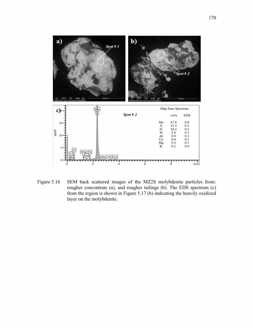
170
Figure 5.16 SEM back scattered images of the MZ2S molybdenite particles from: rougher concentrate (a), and rougher tailings (b). The EDS spectrum (c) from the region is shown in Figure 5.17 (b) indicating the heavily oxidized layer on the molybdenite.
c)

171
Figure 5.17 Magnified SEM micrograph (a) of the molybdenite surface from Spot # 2 shown in Figure 5.16. SEM back scattered electron micrograph of the surface of a molybdenite particle (150x75 µm), isolated from the MZ2S rougher tailings. The EDS spectrum (b) from the region shown in Figure 5.17 (a) indicates that the molybdenite surface was entirely oxidized.
Figure 5.18 SEM image (a) and EDS (b) of a selected chalcopyrite particle, isolated from MZ2S rougher tailings. The corresponding EDS spectrum (b) from the region shown in Figure 5.18 (a) indicate that the chalcopyrite is strongly oxidized due to surface oxidation.

172
.
Figure 5.19 SEM image and EDS of a coarse molybdenite particle, isolated from MZ2S rougher tailings
Figure 5.20 A survey (full range) XPS spectrum of molybdenite particles isolated from the MZ2S and LSE rougher concentrate and tailings.

173
Figure 5.21 High resolution XPS spectra of Mo 3d and S 2s peaks and S 2p peaks, on the MoS2 samples isolated from the LSE (a) and MZ2S (b) samples.
0
0.2
0.4
0.6
0.8
1
1.2
1.4
1.6
224 226 228 230 232 234 236 238
CP
Sx 1
00
00
Binding energy (eV)
LSE - Tailing LSE - Concentrate
Mo 3d3/2
Mo 3d5/2
Mo 3d3/2
S 2s
0
0.2
0.4
0.6
0.8
1
1.2
1.4
1.6
224 226 228 230 232 234 236 238
CP
Sx 1
00
00
Binding energy (eV)
Mz2S - Tailing Mz2S - Concentrate
Mo 3d
Mo 3d3/2
Mo 3d5/2
Mo 3d3/2S 2s
0
0.1
0.2
0.3
0.4
0.5
0.6
160 161 162 163 164 165 166
CP
Sx
1000
0
Binding energy (eV)
Mz2S - Concentrate Mz2S - Tailing
S 2pS 2p3/2
S 2p1/2
S 2p3/2
0
0.1
0.2
0.3
0.4
0.5
0.6
160 161 162 163 164 165 166
CP
Sx
1000
0
Binding energy (eV)
LSE - Tailing LSE - Concentrate
S 2p
S 2p3/2
S 2p1/2
0
0.2
0.4
0.6
0.8
1
1.2
1.4
1.6
224 226 228 230 232 234 236 238
CP
Sx 1
00
00
Binding energy (eV)
LSE - Tailing LSE - Concentrate
Mo 3d3/2
Mo 3d5/2
Mo 3d3/2
S 2s
0
0.2
0.4
0.6
0.8
1
1.2
1.4
1.6
224 226 228 230 232 234 236 238
CP
Sx 1
00
00
Binding energy (eV)
Mz2S - Tailing Mz2S - Concentrate
Mo 3d
Mo 3d3/2
Mo 3d5/2
Mo 3d3/2S 2s
0
0.1
0.2
0.3
0.4
0.5
0.6
160 161 162 163 164 165 166
CP
Sx
1000
0
Binding energy (eV)
Mz2S - Concentrate Mz2S - Tailing
S 2pS 2p3/2
S 2p1/2
S 2p3/2
0
0.1
0.2
0.3
0.4
0.5
0.6
160 161 162 163 164 165 166
CP
Sx
1000
0
Binding energy (eV)
LSE - Tailing LSE - Concentrate
S 2p
S 2p3/2
S 2p1/2
a) LSE ore
b) MZ2S ore
Mo 3d S 1p
Mo 3d S 1p
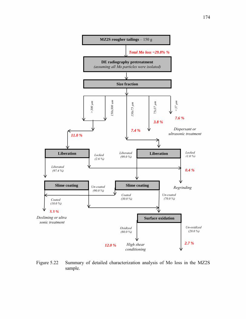
174
Figure 5.22 Summary of detailed characterization analysis of Mo loss in the MZ2S sample.
MZ2S rougher tailings – 150 g
DE radiography pretreatment
(assuming all Mo particles were isolated)
Size fraction
>30
0 µm
150x
300
µm
150x
75 µ
m
75x3
7 µm
<37
µm
7.4 %
3.8 % 7.6 %
11.0 %
Liberation Liberation
Slime coating Slime coating
Total Mo loss =29.8% %
Locked (2.6 %)
Locked (1.0 %)
Liberated (99.0 %)
Liberated (97.4 %)
Coated (10.0 %)
Un-coated (90.0 %)
Coated (30.0 %)
Un-coated (70.0 %)
Surface oxidation
3.3 %
12.0 % 2.7 %
0.4 %
Un-oxidized (20.0 %)
Oxidized (80.0 %)
Desliming or ultra sonic treatment
High shear conditioning
Regrinding
Dispersant or ultrasonic treatment

175
Table 5.1 Scan conditions for the MicroXCT-400 in the analysis of lost particles in KUC rougher tailings samples. Table made by following the scanning procedure of Lin and Miller, 1996
Material
Rougher tailings
1 Objective 4X 2 Total Scan Time hour 4 3 Source Settings (kV/W) kV/Watts 80/10 4 Pixel size (m) µm 4.59 5 Start and End Angle degree 360 6 Number of Views 1000 7 Time per View (sec) second 9 8 Source/Detector Positions mm -44/20 9 Camera Binning 2 10 Physical Filter(glass) µm 150
Table 5.2 CT number distribution/frequency of each mineral phase.
Name
Chemical formula
CT number
original rescaled
1 Air 200 5 2 Silicate SiO2 2000 50 3 Pyrite FeS2 4400 110 4 Chalcopyrite CuFeS2 5040 126 5 Bornite Cu5FeS4 7400 185 6 Molybdenite MoS2 9600 240

176
Table 5.3 Size-by-size chemical analysis for the MZ2HE rougher feed (fine grinding).
Size class, µm
Weight
Assays, %
Distribution, %
gram % Cu Mo Cu Mo 1 >300 7.9 5.2 0.06 0.010 0.6 1.1 2 300x150 36.6 24.4 0.26 0.039 11.8 20.3 3 150x75 38.0 25.3 0.83 0.052 39.4 28.1 4 75x37 35.3 23.6 0.98 0.086 43.4 43.2 5 <37 32.2 21.5 0.12 0.016 4.8 7.2 Total 150.0 100.0 0.53 0.047 100.0 100.0
Table 5.4 Size-by-size chemical analysis for the MZ2HE rougher tailings (fine grinding).
Size class, µm
Weight
Assays, %
Distribution, %
gram % Cu Mo Cu Mo 1 >300 8.1 5.4 0.02 0.008 2.7 6.7 2 300x150 33.8 22.6 0.04 0.016 22.5 54.5 3 150x75 39.8 26.5 0.05 0.005 35.8 21.8 4 75x37 38.8 25.9 0.03 0.002 19.4 8.7 5 <37 29.4 19.6 0.04 0.003 19.6 8.3 Total 150.0 100.0 0.04 0.007 100.0 100.0

177
Table 5.5 Size-by-size chemical analysis for the LSE rougher feed (fine grinding).
Size class, µm
Weight
Assays, % Distribution, %
gram % Cu Mo Cu Mo 1 >300 2.0 1.3 0.67 0.056 1.1 1.7 2 300x150 21.9 14.6 0.47 0.048 8.6 16.2 3 150x75 40.3 26.9 1.10 0.052 35.5 32.6 4 75x37 47.0 31.3 1.09 0.048 43.1 34.8 5 <37 38.8 25.9 0.36 0.024 11.7 14.6 Total 150.0 100.0 0.80 0.043 100.0 100.0
Table 5.6 Size-by-size chemical analysis for the LSE rougher tailings (fine grinding).
Size class, µm
Weight
Assays, % Distribution, %
gram % Cu Mo Cu Mo 1 >300 1.6 1.0 0.28 0.039 3.3 5.6 2 300x150 17.0 11.4 0.15 0.028 19.6 43.1 3 150x75 43.0 28.7 0.06 0.003 20.4 9.9 4 75x37 48.1 32.1 0.06 0.001 22.8 5.7 5 <37 40.3 26.9 0.11 0.010 33.9 35.8 Total 150.0 100.0 0.09 0.007 100.0 100.0

178
Table 5.7 Size-by-size chemical analysis for the MZ2S rougher feed (fine grinding).
Size class, µm
Weight
Assays, % Distribution, %
gram % Cu Mo Cu Mo 1 >300 2.3 1.5 0.22 0.002 0.4 0.1 2 300x150 23.3 15.6 0.35 0.023 6.0 7.7 3 150x75 54.0 36.0 0.95 0.044 37.2 34.7 4 75x37 36.8 24.6 1.70 0.078 45.5 41.9 5 <37 33.6 22.4 0.45 0.032 11.0 15.7 Total 150.0 100.0 0.92 0.046 100.0 100.0
Table 5.8 Size-by-size chemical analysis for the MZ2S rougher tailings (fine grinding).
Size class, µm
Weight
Assays, % Distribution, %
gram % Cu Mo Cu Mo 1 >300 1.7 1.1 0.04 0.003 0.5 0.2 2 300x150 18.4 12.2 0.07 0.025 9.7 23.0 3 150x75 47.4 31.6 0.08 0.019 28.0 44.0 4 75x37 44.3 29.5 0.08 0.005 27.2 10.5 5 <37 38.3 25.5 0.12 0.012 34.5 22.3 Total 150.0 100.0 0.09 0.014 100.0 100.0

179
Table 5.9 The qualitative summary results of liberation characteristics of molybdenite in the rougher tailings of the MZ2HE, LSE and MZ2S ore types.
Ore type Grind condition
Size class, µm
Detected
numbers of molybdenite
Liberation grade, %
0-30 30-50 50-90 90-100
MZ2HE
25 %
+ 1
00 m
esh
300x150 8 2.0 - 12.7 85.3 150x75 14 2.3 2.9 - 94.8
LSE
300x150
68
0.2
1.3
3.0
95.5 150x75 114 0.9 1.5 3.0 94.6
MZ2S
300x150
121 -
2.6
4.1
93.2
150x75 243 0.2 0.7 0.8 98.2
Table 5.10 The binding energy and FWHM values from standard samples of MoS2 and MoO3.
Product
Line BE (eV) FWHM (eV)
MoS2
Mo 3d5/2 229.81 0.42 Mo 3d3/2 232.94 0.63
S 2s 226.99 1.87 S 2p3/2 162.66 0.43
MoO3 Mo 3d5/2 233.15 0.86 Mo 3d3/2 236.28 0.9

180
Table 5.11 Atomic fractions, atomic ratios and the percentages of different Mo and S species with their corresponding totals, derived from the XPS spectra.
Component
LSE ore MZ2S ore
Concentrate Tailings Concentrate Tailings
Atomic fraction (%)
O 56.4 62.5 42.9 73.5 S 24.5 21.0 29.9 18.9
Mo 13.5 11.7 16.4 12.3 Mo4+ 13.0 9.9 14.3 5.2 Mo6+ 0.5 1.8 2.1 7.1
Atomic ratio
S/Mo 1.81 1.80 1.82 1.53 O/S 2.3 3.0 1.4 3.9
O/Mo 4.2 5.4 2.6 6.0
Here 𝑆 = 𝑆2− + 𝑆6+, 𝑎𝑛𝑑 𝑀𝑜 = 𝑀𝑜4+ + 𝑀𝑜6+, respectively

181
CHAPTER 6
CONCLUSIONS
Although mineral resources are nonrenewable, they are indispensable materials for
the development and survival of human societies. The characterization of mineral
resources is a critical component for optimization of the mine-to-mill process, and now
can be accomplished with advanced instrumentation. Each ore body is unique, and has to
be treated as such. The development of advanced characterization technology in recent
years has had direct bearing on the automated analysis systems now available that can
make mineral characterization faster and more accurate. The variability of the feed
quality delivered to flotation plants in mining operations can present challenges to the
operational staff in attempting to achieve satisfactory recovery and grade efficiency.
When faced with variables or difficult ores, plant operators are often required to
implement operational parameter changes to maintain flotation efficiency.
The goal of this research was to improve the understanding of the variables or factors
affecting the flotation efficiency of copper and molybdenum minerals from porphyry
copper ores and to provide some possible solutions to these challenges. Specifically, the
identification and characterization of lost mineral particles using a rapid scan DE
radiography method for the analysis of flotation products was considered to investigate

182
the significance of these problems associated with the flotation efficiency of selected
KUC ore types. According to flotation testing, the Cu and Mo recoveries of some ore
types such as the LSE and MZ2S ore types are far inferior to the more traditional, well-
behaved ore types at the Copperton concentrator, KUC. Significant amounts of Cu and
Mo minerals in these ore types are lost to tailings streams due to many variables that
influence the flotation process and affect the process of mineralization of air bubbles.
These lost trace minerals, mostly unliberated and entrapped in gangue minerals, are
present as fine slimes, or report to tailings due to problems in process operations during
flotation. Tailings evaluation is an area where it is possible to define the actual losses in a
mineral processing plant. However, because of the trace concentrations of these trace
minerals, sample collection and integrity become one of the major concerns in any
project relating to tailings characterization analysis. For a trace mineral such as
molybdenite, the content in the flotation products is in the range of parts per million
(ppm), which means that several millions of particles must be examined to provide
statistical reliabillity, accuracy and confidence in the advanced characterization analysis.
Of course, working with such products is never easy. The process of selecting and
preparing an appropriate, representative sample can be more work than undertaking the
direct characterization analysis.
This research primarily focused on a new radiographic inspection method and
especially the characterization and isolation of lost trace minerals based on measured X-
ray intensities in a relative reflex and the effective atomic number. In particular, an
HRXMT-based technique was developed in order to characterize the lost trace mineral
particles in flotation tailings and/or any other particulate materials. Although the atomic

183
number is well defined for chemical elements, the definition of an atomic number for any
compound is not an easy task. After reviewing the different definition methods available
in the literature, a definition related to the method of X-ray relative reflex measurement
was suggested. For help in determining the relative reflex and the effective atomic
number of unknown minerals, a new concept of mineral identification was introduced in
real flotation practice and advanced mineral characterization analysis. Finally, this
research suggested implementing the accurate, rapid and reliable DE radiographic
inspection method for the isolation of trace mineral particles in flotation products using
an X-ray system. Also, DE radiography inspection is beneficial for characterizing lost
trace mineral particles, and improving data accuracy and reliability of advanced
instrumentation. This especially could reduce sampling errors, experimental cost and
experimental lead time in the plant. As described by Gy (1979), “the failure of mining or
metallurgical undertakings can nearly always be attributed to unaccountable sampling
errors.” This could help researchers to better understand the general characteristics of lost
minerals such as their liberation/exposure state, surface chemistry issues, effect on the
flotation environment and to better control their flotation efficiency. It is expected that in
the near future, DE radiography will be used more and more as a routine research or
sample preparation tool and be successfully integrated with other analytical instruments
in various geological, mining and metallurgical disciplines. In this regard, all objectives
of this research have been achieved.
Tailings from three ore types (LSE, MZ2S and MZ2HE) were characterized in detail
using DE radiography to isolate lost particles. Characterization of the lost particles
according to size was accomplished using optical microscopy, SEM-EDS, XPS and

184
HRXMT and the results used to explain flotation recovery. It was found that copper
losses for each ore type were due to lack of sufficient liberation. Such was not the case
with respect to molybdenum losses. Molybdenum losses for the LSE ore type were found
to be primarily due to slime coating and particle size, whereas molybdenum losses for the
MZ2S ore type were found to be primarily due to surface oxidation and variation in
process water chemistry.

185
APPENDIX A
RESULTS OF FLOTATION TESTING
Table A.1. A summary of the test objectives, conditions and notable results for the rougher kinetic tests.
Test # /
Conditions Product Weight, %
Grade, % Recovery, % Cu Mo Fe Cu Mo Fe
T1a – LSE 25 % + 100
mesh P80 = 168 microns
Ro conc - 1 2.32 31.11 1.25 28.7 72.3 65.0 5.8 Ro conc - 2 0.58 18.92 0.80 20.8 11.3 10.8 1.1 Ro conc - 3 0.27 9.68 0.49 15.7 2.5 2.9 0.4 Ro conc - 4 0.45 6.57 0.46 14.2 2.9 4.6 0.6 Ro tail 96.38 0.11 0.008 10.9 10.9 16.8 92.2 Head calc. 100.00 1.00 0.045 11.5 100.0 100.0 100.0
T2a – LSE 35 % + 100
mesh P80 = 220 microns
Ro conc - 1 1.85 29.7 1.30 27.7 51.9 49.5 4.3 Ro conc - 2 0.75 22.5 0.79 23.7 15.4 11.9 1.4 Ro conc - 3 0.33 14.4 0.59 18.5 4.6 4.1 0.5 Ro conc - 4 0.67 12.8 0.63 18.5 8.6 9.2 1.1 Ro tail 96.40 0.22 0.012 11.2 19.6 25.3 92.6 Head calc. 100.00 1.043 0.048 11.7 100.0 100.0 100.0
T3a – MZ2S 25 % + 100
mesh P80 = 146 microns
Ro conc - 1 2.28 30.5 0.78 23.9 63.6 30.2 32.5 Ro conc - 2 0.87 22.4 1.35 18.0 18.0 20.1 9.4 Ro conc - 3 0.42 11.9 0.93 13.6 4.5 6.6 3.4 Ro conc - 4 0.86 5.36 0.90 7.51 4.2 13.2 3.9 Ro tail 95.58 0.11 0.0 0.89 9.7 29.9 50.8 Head calc. 100.00 1.089 0.059 1.67 100.0 100.0 100.0
T4a – MZ2S 35 % + 100
mesh P80 = 205 microns
Ro conc - 1 2.12 27.60 1.17 22.78 52.9 41.5 27.9 Ro conc - 2 1.08 22.11 1.22 18.54 23.3 23.8 12.5 Ro conc - 3 0.41 14.89 0.98 11.80 5.8 7.1 2.9 Ro conc - 4 0.89 7.76 0.50 7.24 6.3 7.6 3.7 Ro tail 95.50 0.13 0.01 0.92 11.7 20.0 53.0 Head calc. 100.00 1.06 0.057 1.65 100.0 100.0 100.0
T5a – MZ2HE
25 % + 100 mesh
P80 = 120 microns
Ro conc - 1 2.28 18.5 1.53 18.8 65.9 62.8 15.1 Ro conc - 2 1.27 11.2 0.84 13.2 21.6 18.7 5.7 Ro conc - 3 0.58 3.98 0.29 7.20 3.7 3.1 1.5 Ro conc - 4 0.82 1.28 0.11 4.26 1.7 1.6 1.3 Ro tail 95.05 0.05 0.01 2.16 7.2 13.7 76.4 Head calc. 100.00 0.607 0.053 2.69 100.0 100.0 100.0

186
Table A.1 continued
T6a –
MZ2HE 35 % + 100
mesh P80 = 180 microns
Ro conc - 1
2.13
17.3
1.56
18.8
58.0
63.1
14.6
Ro conc - 2 1.03 11.9 0.86 13.0 19.2 16.7 4.9 Ro conc - 3 0.40 5.68 0.38 8.27 3.5 2.9 1.2 Ro conc - 4 0.65 2.11 0.14 5.11 2.2 1.7 1.2 Ro tail 95.80 0.11 0.01 2.24 17.1 15.5 78.2 Head calc. 100.00 0.636 0.053 2.75 100.0 100.0 100.0
Table A.2. A summary of results for the scavenger flotation after desliming.
Test#/ Conditions Product Weight,
% Grade, % Recovery, %
Cu Mo Fe Cu Mo Fe
T1b – LSE Fine grind
Scav. conc 0.92 2.60 0.164 28.99 21.73 25.09 2.53 Scav. tail 68.06 0.05 0.003 11.36 32.87 35.99 73.52 Slime 26.85 0.19 0.009 9.38 45.40 38.91 23.94 Rougher tail. 95.83 0.11 0.006 10.98 100.00 100.00 100.00
T2b – LSE Coarse grind
Scav. conc 0.81 2.19 0.110 14.56 9.72 9.40 1.00 Scav. tail 75.48 0.17 0.009 13.01 70.95 72.61 83.38 Slime 19.60 0.18 0.009 9.39 19.33 17.99 15.62 Rougher tail. 95.89 0.19 0.010 12.28 100.00 100.00 100.00
T3b – MZ2S Fine grind
Scav. conc 1.12 1.74 0.142 3.20 18.26 12.45 3.48 Scav. tail 68.95 0.08 0.012 0.93 50.27 64.72 62.58 Slime 25.51 0.13 0.011 1.37 31.47 22.83 33.94 Rougher tail. 95.58 0.10 0.019 0.89 100.00 100.00 100.00
T4b – MZ2S Coarse grind
Scav. conc 0.96 1.08 0.110 7.11 8.35 10.10 7.76 Scav. tail 73.02 0.12 0.008 0.70 71.39 55.98 57.92 Slime 21.87 0.12 0.016 1.38 20.26 33.92 34.32 Rougher tail. 95.85 0.129 0.011 0.92 100.00 100.00 100.00
T7b – MZ2HE
Fine grind
Scav. conc 0.91 1.46 0.17 5.23 30.48 21.05 2.31 Scav. tail 75.18 0.03 0.011 2.10 51.56 70.06 76.55 Slime 19.62 0.04 0.003 2.22 17.96 8.89 21.14 Rougher tail. 95.710 0.05 0.008 2.15 100.00 100.00 100.00
T8b – MZ2HE
Coarse grind
Scav. conc 1.25 1.11 0.168 6.12 12.33 22.99 3.03 Scav. tail 76.48 0.12 0.007 2.72 78.76 61.96 82.57 Slime 17.62 0.06 0.008 2.10 8.91 15.05 14.39 Rougher tail. 95.35 0.12 0.010 2.64 100.00 100.00 100.00

187
APPENDIX B
RAPID SCAN RADIOGRAPHY SCANNING
PROCEDURE
Sample preparation
Plastic plates (76.2x25.4x1.0 mm) and double-sided sticky tape were used to prepare
the sample for DE radiography scans. First, narrowly sized particles were spread on the
flat surface. Then, the plastic plate with double-side sticky tape on its surface was tapped
on the particle bed. Finally, a single layer of particles was stabilized with the second
plastic plate.
Scanning operating procedures
The XRadia Micro XCT-400 is the main operating device of the experiments in rapid
scan radiography. Standard operating procedure will be discussed step-by-step in order to
convey a general idea of the HRXMT scan operation:
Click the Start button and open XMController 7.0.2817
Go to the X-RAY SOURCE DIALOG box as shown in Figure B.1 and click ON. The
red light on the top of the machine will turn on while the X-ray source is powered.
Voltage and power can be adjusted. In this study, high- (140 kV) and low- (80 kV)

188
energy level will be used for dual energy radiography with 10 W power. Clicking ON
or APPLY will switch the machine to Standby mode (fully warmed up) or Warming
up mode. The warming up process will take 15 minutes.
During the warming up process, the sample material is being prepared and fastened
onto the sample holder and also check the filter in the filter holder. In this case, we
used a 150 µm glass filter for reducing a specific element effect.
The red light on the top of the machine will shut off after the machine is fully warmed
up. Open the chamber and put the sample with the holder on the stage. Close the
chamber and check if the green light is on.
Check and adjust the MAGNIFICATION LEVEL; it should be 4X, as shown in
Figure B.2.
Go to the X-RAY SOURCE DIALOG box and click on the X-Ray On button again.
This time the machine reaches a specific power level in only a few seconds after
being fully warmed up. Set up voltage and power to first selected level (voltage - 140
kV and power - 10W) and click APPLY. The machine will raise the energy the
selected level in a few seconds. When the power is raised to the selected level, turn on
the internal light and the surveillance camera.
Open the MOTION CONTROLLER window, as shown in Figure B.3; adjust
distances of source and detector. In this case, the scan conditions are set at 4X
magnification with 5 second exposure time; source voltage is set at 140kV; distance
between source and detector is -44 mm and 20mm; camera binning is set at 2 with a
150 µm glass filter.
Go to the ACQUISITION SETTING dialog box and select Continuous Scan with 1

189
second exposure time, binning 4, as shown in Figure B.4. Keep the rest of the
settings unchanged and press the START ACQUISITION button. This step will
acquire an initial position of projections for field of view calibration. The sample
image will be acquired and refreshed every second (depending on the exposure time).
Binning 4 helps to reduce the file size and the image acquisition time, however, it
loses the pixel resolution and increases X-ray intensity on the detector.
Go to the MOTION CONTROLLER window and select SAMPLE section. The
sample itself can move on the x axis (from door side to inner side), y axis (sample
raises or descent) in micron precision. Find the pinhole, which is on the sample slide
and click on the center of pinhole.
Go to VIEW and click Highlight Center of FOV; a central cross line will show up
and indicate the center of the pinhole image. Move the field of view from pinhole to
the region of interest (initial position of first radiography image) by double clicking
the left mouse key on the acquired image shown in Figure B.3. Make sure the region
of interest is covered by the sample as much as possible on field of view. The field of
view will be reallocated to a new central point on which the cursor clicks. The field of
view can be also adjusted by pushing forward or pulling back the joystick on the
control panel. If the field of view is well calibrated, then press STOP in the icon bar.
Then write down an initial coordinate in the MOTION CONTROLLER on your
student note or blank sheet.
Go to the ACQUISITION SETTING dialog box again and select the AVERAGING
mode this time. Image noise can compromise the level of detail in the radiography
images, so reducing this noise can greatly enhance our final image. The exposure

190
time is set at 5 seconds according to the applied CT standard for the scan. The
binning is set at 2 for a regular scan. Keep the rest of the settings unchanged and press
the START ACQUISITION button. This step will provide a single radiographic
image.
If the image quality and scan conditions are satisfactory for the scan requirements, the
SAVE AS window will automatically open after pressing the START
ACQUISITION, save this image and name the image:
LSE_fine_p100_slide_1_N1_Se1x1_HE.xrm.
The naming rule, here is followed by Ore type, Grind condition, Slide #, Test #,
Section #, and Energy level. Click the SAVE button to start the scan.
The scanning process will take 25 - 40 seconds depending on averaging numbers (3-5
images).
Go to the X-Ray Source dialog box again and set up voltage to second selected level
(voltage - 80 kV and power – 10W). This time the machine reaches a specific power
level in only a few seconds. Wait 60 seconds for stabilizing energy output in the
machine.
Go to the ACQUISITION SETTING dialog box and select AVERAGING again.
Keep the rest of the settings unchanged except voltage and press START
ACQUISITION. The scanning process will also take 25 - 40 seconds, same as the
previous scan.
If the image quality and scan conditions are satisfactory, save this image and name it
LSE_fine_p100_slide_1_N1_Se1x1_LE.xrm. Now we have two images with the
same coordinate and same scan conditions, both a high- (140 kV) and a low- (80 kV)

191
energy level.
After the scanning process at high- and low-energy levels establish averaged
references (Figure B.5.). It should be prepared on both high- and low- energy level.
Go to the Image controls window and click the REFERENCE button and then choose
the BROWSE section. The OPEN FILE window will be automatically opened after
choosing BROWSE section. To apply the reference with the same scan condition to
interest of point (radiographic image).
After applying reference into interest of point, go to File and click on Export and it
will then open the SAVE FILE window. We need to convert file type from *.xrm to
*.bin, as shown in Figure B.6 for image data analysis.
Reference preparation
Because the environment for the HRXMT scan is neither in a vacuum nor isolated,
reference states are measured to remove X-ray attenuation of background, air and other
effects associated with the lens like dirty spots and dust. The reference can be shot before
or after the scan following the same scan condition. Each sample (slide) should have their
own references both on high- and low-energy level; save them on the same folder with
sample scans. Reference preparation procedure will be discussed step-by-step in order to
convey a scan operation:
Go to the X-RAY SOURCE DIALOG box and click on the X-Ray Off button if the
X-ray source did not turn off. Then, the orange light on the top of the machine will
turn off;
Remove a sample with holder from stage;

192
Go to the X-RAY SOURCE DIALOG box and click on the X-Ray On button, again.
The orange light on the top of the machine will turn on. Make sure the scan
conditions are set the same as high-energy level at 4X magnification with 5 second
exposure time; source voltage is set at 140kV; distance between source and detector
are -44 mm and 20mm; camera binning is set at 2 with a 150 µm glass filter and click
APPLY. This time the machine reaches a specific power level in only a few seconds;
Go to the ACQUISITION SETTING dialog box and select AVERAGING. Then
press the START ACQUISITION button and save this reference and name it:
LSE_fine_p100_slide_1_N1_ reference_140kV.xrm;
Repeat steps 1-5 for the second reference for low-energy level but remember to
change voltage to 80 kV and keep the rest of the settings unchanged;
Save this reference and name the image:
LSE_fine_p100_slide_1_N1_reference_ 80kV.xrm.

193
Figure B.1 The X-Ray source dialog icon.
Figure B.2 The magnification icon in the XMController.

194
Figure B.3 The acquisition setting, motion control, image control window.
Figure B.4 The acquisition control setting in the continuous mode.

195
Figure B.5 Image control setting.
Figure B.6 Reference applying method.

196
APPENDIX C
MATHLAB CODE - RAPID SCAN RADIOGRAPHY
clear; clc; close all; Size = 1014; p=3.8;
%% HE
fid = fopen('../../Zeff on standard/Mo_Pb_Cu_Al_Si_Au
standard_HER.bin','rb');
HER = fread(fid, Size * Size,'float32'); fclose(fid);
fid = fopen('../../Zeff on standard/Mo_Pb_Cu_Al_Si_Au
standard_HE.bin','rb');
HE = fread(fid, Size * Size,'float32'); fclose(fid);
HE = reshape(log(HER./HE), Size, Size);
PbH=HE(700:760,600:660); mPbH=mean(PbH(:));
CuH=HE(650:710,350:410); mCuH=mean(CuH(:));
AlH=HE(390:440,260:440); mAlH=mean(AlH(:));
%% LE
fid = fopen('../../Zeff on standard/Mo_Pb_Cu_Al_Si_Au
standard_LER.bin','rb'); LER = fread(fid, Size * Size,'float32'); fclose(fid);
fid = fopen('../../Zeff on standard/Mo_Pb_Cu_Al_Si_Au

197
standard_LE.bin','rb'); LE = fread(fid, Size * Size,'float32'); fclose(fid);
LE = reshape(log(LER./LE), Size, Size);
PbL=LE(720:780,600:640); mPbL=mean(PbL(:));
CuL=LE(650:730,350:440); mCuL=mean(CuL(:));
AlL=LE(360:430,260:440); mAlL=mean(AlL(:));
%% Determination of relative reflexes =(X1, X2, X3) of standart samples
X1=mPbL/mPbH
X2=mCuL/mCuH
X3=mAlL/mAlH
%% Determination of coefficients ( k1, k2, k3, k4) of Equation # 15
Z1=82^p; Z2=29^p; Z3=13^p;
k1=Z1*Z2*(X1-X2)-Z1*Z3*(X1-X3)+Z2*Z3*(X2-X3)
k2=X1*X2*Z3*(Z1-Z3)-X1*X3*Z2*(Z1-Z3)+X2*X3*Z1*(Z2-Z3)
k3=X1*(Z2-Z3)-X2*(Z1-Z3)+X3*(Z1-Z2)
k4=X1*X2*(Z1-Z2)-X1*X3*(Z1-Z3)+X2*X3*(Z2-Z3)
%% Isolation and identification of unknown minerals based on the relative reflex (Zeff sample)
for i=1:1
for j=1:1
name=sprintf('LSE_fine_p100_slide_1_N1_Se%ix%i_HE.bin', i, j);
fid=fopen(name,'rb');
HE=fread(fid, Size * Size,'float32');
fclose(fid);

198
name=sprintf('LSE_fine_p100_slide_1_N1_Se%ix%i_LE.bin', i, j);
fid=fopen(name,'rb');
LE=fread(fid, Size * Size,'float32');
fclose(fid);
X=(LE)./(HE);
Zeff=((k1*X+k2)./(k3*X+k4)).^(1/p);
Zeff = reshape(Zeff, Size, Size);
figure,imshow(Zeff,[0,50]);colormap(lines);
name=sprintf('Zeff_%ix%i.bin',i,j);
fid=fopen(name,'wb');
fwrite(fid,Zeff,'float32');
fclose(fid);
disp([num2str(i),'',num2str(j)])
end
end

199
REFERENCES
Alvarez, R.E., and Macovski, A. 1976. Energy selective reconstructions in X-ray computerized tomography. Phys. Med. Biol. 21: 733-744.
Alvarez, R.E., Seibert, J.A., and Thompson, S.K. 2004. Comparison of dual energy
detector system performance. Med Phys. 3: 56-65. Ametov, I., Grano, S.R., Zanin, M., Gredelj, S., Magnuson, R., Bolles, T., Triffett, B.,
Zuo, W.D., Yao, S.C., Liang, W.F., Cheng, Z.L., and Long, H. 2008. Copper and molybdenite recovery in plant and batch laboratory cells in porphyry copper rougher flotation. Proceedings of XXIV IMPC, Beijing, China. 1: 1129–1137.
Arnold, B.J., and Aplan, F.F. 1986. The effect of clay slimes on coal flotation, part ii: the
role of water quality. Int. J. Miner. Process. 17 (3–4): 243–260. Babcock, R.C., Ballantyne, G., and Phillips, C. 1997. Summary of the geology of the
Bingham District, Utah. Geology and ore deposits of the Oquirrh and Wasatch mountains. Utah Society of Economic Geologists.
Barzyk, W., Malysa, K., and Pomianowski, A. 1981. The influence of surface oxidation
of chalcocite on its floatability and ethyl xanthate sorption. Int. J. Miner. Process. 8 (1): 27–29.
Basilio, C.I., Kartio, I.J., and Roon, R.H. 1996. Lead activation of sphalerite during
galena flotation. Miner. Eng. 9: 869–879. Bradshaw, D.J., Triffett, B., and Kashuba, D. 2011. The role of process mineralogy in
identifying the cause of the low recovery of chalcopyrite at KUC. Proceedings of X ICAM. Trondheim, Norway, 73-80.
Briggs, D., and Seah, M.P. 1990. Practical Surface Analysis: Auger and X-ray
photoelectron spectroscopy. John Wiley & Sons. Brody, W.R., Butt G., Hall A., and Macovski, A.A. 1981. Method for selective tissue and
bone visualization using dual-energy scanned projection radiography. Med. Phys. 8 (3): 353–357.

200
Broman, P.G. 1980. Water reuse at sulfide ore concentrators in Sweden: practice, experience and current development. Jones, M.J. Ed. Complex Sulphide Ores. The Institution of Mining and Metallurgy, London. 28–39.
Brown, A.M. 2001. Step-by-step guides to nonlinear regression analysis of experimental
data using a Microsoft excel spreadsheet. Computer Methods Programs in Biomedicine. 65: 191-200.
Brozek, M., and Mlynarczykowska, A. 2006. Analysis of kinetics models of batch
flotation. Physicochemical Problems of Mineral Processing. 41: 51–65. Bulatovic, M. 2007. Handbook of flotation reagents: chemistry, theory and practice:
Flotation of sulphides ores. Elsevier Scientific Pub. Co. Bulled, D., and McInnes, C. 2005, Flotation plant design and production planning
through geometallurgical modeling. Centenary of Flotation Symposium, Brisbane, QLD. 6-9.
Canepa, C., and Bernuy, O. 1981. Mineral beneficiation and ore microscopy, some
relevant methodological aspects. Proceedings of Process Mineralogy, The Metallurgical Soc. of AIME. 191-200.
Cardinal, H.N., and Fenster, A. 1990. An accurate method for direct dual energy
calibration and decomposition. Med. Phys. 17: 327. Castro, S., Venegas, I., Landero, A., and Laskowski, J. 2010. Frothing in seawater
flotation systems. Proceedings of XXV IMPC 2010, Brisbane, Australia. 4039–4047.
Celik, M.S. 1988. Effect of ultrasonic treatment on the floatability of coal and galena, J.
Sep. Science and Technology. 24 (14): 1159-1166. Chander, S. 1999. Fundamentals of sulfide mineral flotation, in advances in flotation
technology. Parekh . B.K., and Miller J.D, Ed. Society of Mining, Metallurgy and Exploration, Inc., Littleton, Colorado, 129-165.
Chander, S., and Fuerstenau, D.W. 1974. The effect of potassium diethyldithiophoshate
on the interfacial properties of molybdenite. Trans. Inst. Min. Met. 83: C180-C185
Changlian. X.1985. Kinetic models for batch and continuous flotation in a flotation
column. Proceedings of XV IMPC, Cannes, 3: 16-27. Coleman, R.G., Urtubia, H.E., Alexander, D.J., and Bailey, C.W. 2007. Integrated
grinding and flotation simulations for the improvement of circuit performance at BHB-Billiton’s Minera Escondida. Proceedings of XXXIX Annual Canadian Mill

201
Operators Conference, Ottawa, Canada. Crozier, R.D. 1979. Flotation reagent practice in primary and by-product molybdenite
recovery. Mining Magazine. 140: 174-178. Crozier, R.D. 1992, Flotation, theory, reagents and ore testing. Permagon Press. Das, A.S., Ratnakar Sahu, K.K., and Goswami, N.G. 2008. Importance of mineralogy in
mineral processing. Training course on mineral processing and nonferrous extractive metallurgy. Jamshedpur, India.
Davy, P.J. 1984. Probability models for liberation. Journal of Applied Probability. 21(2):
260-269. Favretto, S. 2009. Applications of X-ray computed micro tomography to material science,
devices and perspectives. PhD dissertation, Universita of Degli Studi de Trieste. FLSmidth Technical Report. 2012. Rio Tinto – Kennecott Utah Copper. Cornerstone
project. Results of phase I flotation variability testing on the Bingham pit south pushback expansion including 32 core samples and 6 surface composite samples.
Forssberg, K.S.E., Jönsson, H.R., and Pualsson, B.I. 1985. Full scale test of process water
reuse in a complex sulphide ore circuit. Forssberg, K.S.E. Ed. Flotation of Sulphide Minerals. Elsevier Scientific Pub. Co, Amsterdam, Netherlands. 197-217.
Fuerstenau, D.W. 2005, A century of developments in the chemistry of flotation
processing. Centenary of Flotation Symposium. Brisbane, Australia. 245-301. Fuerstenau, D.W. 2007. A century of developments in the chemistry of flotation
processing. Froth Flotation: A Century of Innovation, SME, Denver, USA. 1–13. Fuerstenau, D.W., and Chander, S. 1972. On the natural floatability of molybdenite.
Transactions SME. 255 (1): 62-69. Fuerstenau, D.W., and Herrera-Urbina, R. 1989. Mineral separation by flotation:
Surfactant based separation process. Edited by Scamehorn J.F. and Harwell, J.H., New York, Marcel Dekker.
Fuerstenau, M.C. 1982. Sulphide mineral flotation, in principles of flotation. R.P. King,
Ed. Proceedings of SAIMM, Johannesburg. 159-182. Fuerstenau, M.C. 2003. Principles of mineral processing. SME Publications. Fuerstenau, M.C., Miller, J.D., and Kuhn, M.C. 1985. Chemistry of flotation. Society of
mining, Metallurgy and Exploration, Inc. Littleton, Colorado, 74-78.

202
Fullston, D., Fornasiero, D., and Ralston, J. 1999. Zeta potential study of the oxidation of copper sulfide minerals, physicochemical and engineering aspects. Colloids and Surfaces. 146-113.
Garcia, D., Lin, C.L., and Miller, J.D. 2009. Quantitative analysis of grain boundary
fracture in the breakage of single multiphase particles using X-ray microtomography procedures. Miner. Eng. 22: 236.
Gauntt, D.M., and Barnes, G.T. 1994. X-ray tube potential, filtration, and detector
considerations in dual-energy chest radiography. Med. Phys. 21, 203–218. Gay, S.L., and Latti, A.D. 2006. Representation of particle multi-mineral distributions.
Proceedings of XXII IMPC. Istanbul, Turkey. Gerson, A.R., Smart, R.S.C., Li, J., Kawashima, N., Weedon, Triffett, D., and Bradshaw,
D. 2012. Diagnosis of the surface chemical influences on flotation performance: copper sulfides and molybdenite. Int. J. Miner. Process. 106–109, 16–30.
Goodall, W.R., Scales, P.S., and Butcher, A.R. 2005. The use of QEMSCAN and
diagnostic leaching in the characterization of visible gold in complex ores. Miner. Eng. 18: 877-886.
Grano, S., Zanin, M., and Ametov, I. 2009. A study of mechanisms affecting molybdenite
recovery in a bulk copper-molybdenum flotation circuit. Int. J. Miner. Process. 93: 256-266.
Greet, C., and Smart, R.St.C. 1996. The effect of size separation by cyclosizing and
sedimentation on mineral surfaces. Miner Eng, in press. Gribble, C.D., and Hall, A.J. 1992. Optical mineralogy, principles and practice. UCL
Press. London. Gu, Y. 2003. Automated scanning electron microscope based mineral liberation analysis
an introduction to JKMR/FEI mineral liberation analyzer. J. Minerals and Materials Characterization and Engineering, 2 (1): 33 - 41.
Gu,Y., and Napier-Munn, T. 1997. JK/Philips mineral liberation analyzer – an
introduction. In Minerals Processing '97 Conf. Cape Town, SA. Guy, P.J., and Trahar, W.J. 1984. The influence of grinding and flotation environments
on the laboratory batch flotation of galena. Int. J. Miner. Process. 12: 15. Gy, P.M. 1979. Sampling of particulate materials: theory and practice. Elsevier
Scientific Pub. Co. Harris, C.C. 1976. Flotation machines, in Flotation, A.M. Gaudin Memorial, Fuerstenau

203
M.C. Ed. Proceedings of AIME. New York, 753-815. Heaven, T.J., Sharon L., White, David, M., Gauntt, Richard, A., Weems., Mark, S., and
Litaker. 2010. Density measurements of dentin by dual-energy radiography. J. Dent. Edu. 109 (4):604-14.
Herrera-Urbina, R. 2003. Recent developments and advances in formulations and
applications of chemical reagents used in froth flotation. Mineral Processing and Extractive Metallurgy Review. 24 (2): 139-182.
Herrera-Urbina, R., F.J. Sotillo,. and Fuerstenau, D.W. 1999. Effect of sodium sulfide
additions on the pulp potential and amyl xanthate flotation of cerussite and galena, Int. J. Miner. Process. 55 (3): 157.
Hsieh, C.H. 2012. Procedure and analysis of mineral samples using high resolution X-
ray micro tomography, MS thesis, University of Utah, Salt Lake City, Utah, USA. Huynh, L., Feiler, A., Michelmore, A., Ralston, J., and Jenking, P. 2000. Control of slime
coatings by the use of anionic phosphates, a fundamental study. Miner. Eng. 13 (10-11): 10591069.
ICSG. 2014. The world copper factbook. International Copper Study Group.
http://www.icsg.org/ Accessed 12/20/2014. ImageJ. 2011. Image processing and analysis in Java. National Institutes of Health.
http://rsb.info.nih.gov/ij/index.html. Accessed 12/30/2014. Imaizumi, T., and Inoue, T. 1963. Kinetic consideration of froth flotation. Proceedings of
the VI IMPC. Pergamon Press, Cannes. Kahn, S.L., and Gaskin, C. 2012. Radiographic atlas of skeleton maturation. Lippincott
Williams & Wilkins, Thieme Medical publishers, Inc. Kennecott Utah Copper, Rio Tinto Annual Report. http://www.kennecott.com Accessed
3/15/2014. King, R.P. 1982. The prediction of mineral liberation from mineralogical texture.
Proceedings of XIV IMPC. Toronto, Canada, 11-7. King, R.P., and Schneider, C.L. 1993. An effective SEM-based image analysis for
quantitative mineralogy. KONA. 11: 165-177. King, R.P., and Schneider, C.L. 1998. Stereological correction of linear grade
distributions for mineral liberation. Powder Technol. 98: 21-37 Klimpel, R.R., and Hansen, R.D. 1988. Frothers, in reagents in mineral technology. P.

204
Somasundaran, B.M. Moudgil, Marcel Dekker, New York. 385 – 409. Klimpel, R.R., Dhansen, R, and Fee, B.S. 1986. Selection of flotation reagents for
mineral flotation. In Design and installation of concentration and dewatering circuit. Mular, AL Ed. 26: 384-404.
Kniss, J., Kindlmann, G., and Hansen, C. 2001. Interactive volume rendering using
multidimensional transfer functions and direct manipulation widgets. Proceedings of IEEE Visualization. 1: 255-262.
Laskowski, J.S., and Castro, S. 2008. Flotation in concentrated aqueous electrolyte
solutions. Proceedings of XI IMPC. Antalya, Turkey, 281–290. Lazic, P., and Calic, N. 2000. Boltzmann’s model of flotation kinetics, Proceedings of
XXI IMPC. Rome, Italia. B (8): 87-93. Leavay, G., Smart, R., and Skinner, W.M. 2001. The impact of water quality on flotation
performance. J. S. Afr. Inst. Min. Metall. 101. Lehmann, L.A., Alvarez, R.E., Macovski, A., Brody, W.R., Pelc, N.J., Rieder, S.J., and
Hall, A.L. 1981. Generalized image combinations in dual KVP digital radiography, Med. Phys. 8 (5).
Leja, J. 1982. Surface chemistry of froth flotation, Plenum Press. New York, 758. Lenkovskaya, G.L., and Stepanov, B.A. 1969. Effect of the ion composition of the pulp
on molybdenite floatation. Chem. Abstr. 71: 155-222. Limaye, A. 2006. Drishti-volume exploration and presentation tool. Poster presentation.
Baltimore. Lin, C.L. 1987. Measurement and prediction of mineral liberation during grinding. PhD
dissertation. University of Utah, Salt Lake City, Utah. USA. Lin, C.L., and Miller, J.D. 1996. Cone beam X-ray micro tomography for three-
dimensional liberation analysis in the 21st century. Int. J. Miner. Process. 47: 61-73.
Lin, C.L., and Miller, J.D. 2001. A new cone beam X-ray micro tomography facility for
3D analysis of multiphase material. Proceedings of II Proceedings of VI WCIPT. Hannover, Germany.
Lin, C.L., Hsieh, C.H., Tserendagva, T., and Miller, J.D. 2013. Dual energy rapid scan
radiography for geometallurgy evaluation and isolation of trace mineral particles. Miner Eng. 40: 30-37.

205
Lin, C.L., Miller, J.D., Herbst, J.A., and Rajamani, K. 1987. Comparison of methods for the measurement of linear grade distributions in liberation analysis. Particle and particle systems characterization. 4, 78-82.
Lin, C.L., Miller, J.D., Hsieh, C.H., Tiwari, P., and Deo, M.D. 2010. Pore scale analysis
of oil shale pyrolysis by X-ray CT and LB simulation. Proceedings of VI WCIPT. Beijing, China.
Liu, L., Rao, S.R., Finch, J.A. 1993. Technical note: laboratory study effect of recycle
water on flotation of a Cu/Zn sulphide ore. Miner. Eng. 6 (11): 1183 – 1190. Maksimov, I.I., and Emeljanov, I.I. 1983. The effect of turbulence on detachment process
in the flotation pulp. Obogascenie rud. 2: 16-19. Martensen, K.M. 2010. Radiographic Image Analysis. Elsevier Scientific Pub. Co -
Health Sciences Division. MathLab. 2012. Bioinformatics Toolbox. User's Guide . http://www.mathworks.com/ McAuliffe, M.J., Francois, M., and Lalonde. 2012. Medical image processing, analysis &
visualization in clinical research, Proceedings of XXVI International Symposium on Computer-Based Medical Systems National Institutes of Health. Bethesda, Maryland.
McCullough, E.C. 1975. Photon attenuation in computed tomography. Med Phys. 2: 307-
320. Mckinsey Global Institute, Preparing for China’s urban billion. Accessed 3/1/2009. Medina, J.H. 2012. Liberation-limited grade/recovery curves for auriferous pyrite ores as
determined by high resolution X-ray Microtomography. PhD dissertation. University of Utah.
Miller, J.D. 2012. Advances in X-ray tomography in the processing of mineral resources,
Proceedings of XXVI IMPC. New Delhi, India Miller, J.D., and Lin, C.L. 1988. Treatment of polished section data for detailed liberation
analysis. Int. J. Miner. Process. 22: 41-58. Miller, J.D., and Lin, C.L. 2004. Three-dimensional analysis of particulates in mineral
processing systems by cone-beam X-ray micro tomography, Minerals and Metallurgical Processing. 21: 113-124.
Miller, J.D., and Lin, C.L. 2009. High resolution X-ray micro CT (HRXMT) – advances in 3D particle characterization for mineral processing operations. Mineral processing plant design. Ventana Canyon Resort, Tucson, Arizona.

206
Miller, J.D., and Lin, C.L. 2013. 3D characterization, analysis, and simulation of multiphase systems using high resolution X-ray micro tomography. First International Meeting, Metallurgy, Lima, Peru.
Miller, J.D., and Lin, C.L., Al-Wakeel, M.I., Hupka, L. 2009. Liberation-limited
grade/recovery curves from X-ray micro CT analysis of feed material for the evaluation of separation efficiency, Int. J. Miner. Process. 93 (1): 48–53.
Miller, J.D., Lin, C.L., Videla, A., and Medina, J.H. 2009. Three dimensional liberation
analysis of feed and products from copper flotation circuits using high-resolution X-ray micro CT (HRXMT). Proceedings of VI IMPC. Santiago, Chile.
Mineral Resources Authority of Mongolia. 2012. Industrial minerals and selected rare
metals in Mongolia. Investor’s guide. Mineral Resources Authority of Mongolia. 2012. Mongolia—the land of opportunities:
Ulaanbaatar, Mongolia. Mineral Resources Authority of Mongolia, 30. Minitab Statistical Software Features-Minitab. Software for statistics, process
improvement. http://www.minitab.com/en-US/products/minitab/. Accessed 4/11/2011.
MIPAV, 2007. Medical image processing, analysis and visualization, National Institutes
of Health, http://mipav.cit.nih.gov/. Mongolian Extractive Industries Transparency Initiative, 2010. Proceedings of V EITI
Reconciliation Report. Ulaanbaatar, Mongolia, http://www.eitimongolia.mn. Muganda, S., Zanin, M., and Grano, S.R. 2011. Influence of particle size and contact
angle on the flotation of chalcopyrite in a laboratory batch flotation cell. Int. J. Miner. Process. 98 (3-4): 150-162.
Muzenda, E. 2010. An investigation into the effect of water quality on flotation
performance, Proceedings of WASET 45: 237-241. National Institutes of Health. Image processing and analysis in Java.
http://rsbweb.nih.gov/ij/. Accessed 5/24/2014 National Statistical Office of Mongolia, 2012, Monthly bulletin of statistics. National
Statistical Office of Mongolia, December, 133p. Naydenov, S.V., and Ryzhikov,V.D. 2002. Determining chemical compositions by
method of multi-energy radiography. Technical Physics Letters. 28: 357-360. Naydenov, S.V., and Ryzhikov,V.D. 2003. Multi-energy techniques for radiographic
monitoring of chemical composition: theory and applications. Nuclear Instrum

207
and Meth. A (505): 556-558. Naydenov, S.V., Ryzhikov,V.D., and Seminozhenko,V.P. 2002. Multi-energy approach
in non-destructive testing of functional materials. Reports of NANU. 11: 95-100. Naydenov, S.V., Ryzhikov,V.D., and Smith, C.F. 2003. Direct reconstruction of the
effective atomic number of materials by the method of multi-energy radiography. Nuclear Instrum and Meth. B (215): 552-560.
Naydenov, S.V., Ryzhikov,V.D., and Smith, C.F. 2006. Multi-energy ZnSe-based
radiography against terrorism: theory and experiments. Proceedings of SPIE 6319. A1-A8.
Nelson, S. 2007. Kennecott Utah Copper. Internal email communication. NIST (National Institute of Standards and Technology) Nowotny, R. 1998, XMuDat: photon attenuation data on PC, Tech. Rep. IAEA. Vienna,
Austria, https://www-nds.iaea.org/publications/iaea-nds/iaea-nds-0195.htm. Peng, Y., and Grano, S. 2010. Effect of iron contamination from grinding media on the
flotation of sulphide minerals of different particle size. Int. J. Miner. Process. In press. Corrected proof.
Raghavan, S., and Hsu, L.L. 1984. Factors affecting the flotation recovery of
molybdenite from porphyry copper ores. Int. J. Miner. Process. 12(1–3): 145–162.
Ralph., and Chau. 1993. Jolyon & Katya Ralph's Mindat Home Page. Online database,
http://en.wikipedia.org/wiki/mindat.org. Rao, S.R., and Finch, J.A. 1989. A review of water re-use in flotation. Miner. Eng. 2 (1):
65–85. Rasband, W.S. 1997-2014. ImageJ, U. S. National Institutes of Health, Bethesda,
Maryland, USA, http://imagej.nih.gov/ij/. Rey, M., and Raffinot, P. 1966. Flotation of ore in seawater: high frothing, soluble
xanthate collecting. World. Min. 18. Rio Tinto Annual Report. 2014. http://www.riotinto.com/annualreport2013/ Accessed
3/5/2014. Rio Tinto. 2014. Copper fact sheet, Rio Tinto, Eastbourne Terrace, London, United
Kingdom.

208
Roman, L.A. 2008. Limitations to recovery in the flotation of sulfide ores. MS thesis, University of Utah, Salt Lake City, Utah, USA.
Runge, K.C., Dunglison, M.E., Manlapig, E.V., and Franzidis, J.P. 2001. Floatability
component modeling–a powerful tool for flotation circuit diagnosis. Proceedings of the IV UBC-McGill-UA, 93-107.
Runge, K.C., McMaster, J.K., Ijsselstijn, M., and Vien, A. 2007. Establishing the
relationship between grind size and flotation recovery using modeling techniques. Proceedings of IMPC. Cape Town.
Ryzhikov V.D., Naydenov S.V., Grinyov B.V., Lisetskaya E.K., Kozin D.N., Opolonin
A.D., and Starzhinskiy N.G. 2003. Multi-energy radiography on the basis of scintillator–photodiode detectors. Nuclear Instrum and Meth. 549–551.
Santana, R.C. 2008. Influence of particle size and reagent dosage on the performance
of apatite flotation, Separation and Purification Technology. 64: 8-15. Schena, G., Chiaruttini, C., Dreossi, D., Olivo, A., and Pani, S. 2002. Grade of fine
composite mineral particles by dual-energy X-ray radiograph. Int. J. Miner. Process. 67: 101-122.
Schena, G., Dreossi, D., Montanari, F., Olivo, A., and Pani, S. 2003. Multiple-energy X-
ray radiography and digital subtraction for a particle-composition sensor. Miner. Eng. 16: 609-617.
Schneider, C.L. 1995. Measurement and calculation of liberation in continuous grinding
circuits. Ph.D dissertation, University of Utah. Schneider, C.L. 2003. Prediction of liberation from unbroken 3-phase texture: a case
study on a coal sample, Proceedings of XXII IMPC. Senior, G.D., and Trahar, W.J. 1991. The influence of metal hydroxides and collector on
the flotation of chalcopyrite. Int. J. Miner. Process. 33: 321–341 Shirley, J.F., and Sutulov, A. 1985. By-product molybdenite. Weiss, N.L. (Ed.), SME
Mineral Processing Handbook. AIME, New York, 16-17 and 16-36. Sillitoe, R., and Petersen, R. 1996. Andean copper deposits: New discoveries,
mineralization, styles and metallogeny. Littleton, CO, USA. SME, 2012, Theory and practice of sampling particulate materials. Elsevier Scientific
Pub. Co. SNL-Metals Economic Group. 2013. Worldwide exploration trends.
http://go.snl.com/rs/snlfinanciallc/images/MEG_WETbrochure2013.pdf.

209
Accessed 10/22/2014. SolGold. 2014. SolGold Annual Report. http://www.solgold.com.au/page/investor-
centre/annual-reports/. Accessed 11/07/2014. Spevak, P. 1993. Chemistry of molybdenum oxide and sulphide surfaces. PhD
dissertation, University of Western Ontario. Sutherland, D.N. 1998. Application of quantitative process mineralogy through the
mining cycle, Proceedings of AusIMM Annual Conference - 98. Mount Isa, 333 – 337.
Szatkowski, M., and Freyberger, W.L. 1985. A model describing mechanism of flotation
process. Transactions of the Institution of Mining and Metallurgy. C (94): C129-C135.
Szatkowski, M., and Freyberger, W.L. 1985. Kinetics of flotation with fine bubbles.
Transactions of the Institution of Mining and Metallurgy. C (94): C61-C70. Taylor, P.R., Spiller, E., Levier, M., and Melhotra, D. 2009. 3D Particle characterization
for mineral processing operations. Recent advances in Mineral Processing Plant Design. SME: 48-59.
Trahar, W.J. 1981. A rational interpretation of the role of particle size in flotation. Int. J.
Miner. Process. 8: 289–327. Trahar, W.J., and Warren, L.J. 1976. The floatability of very fine particles-a review, Int.
J. Miner. Process. 3: 103-131. Triffett, B., and Bradshaw, D. 2008. The role of morphology and host rock lithology on
the flotation behavior of molybdenite at Kennecott Utah Copper. AusIMM Publication Series, Proceedings of IX ICAM. 465-473.
Triffett, B., Veloo.C., Adair,B.J.I., and Bradshaw, D. 2008. An investigation of the
factors affecting the recovery of molybdenite in the Kennecott Utah Copper bulk flotation circuit, Miner. Eng. 21: 832–840.
US patent. 2000. Method and an apparatus for analyzing a material. Technological
Resources Pty Limited. http://patents.com/us-6122343.html. Accessed 2/15/2015. USGS, 1996-2014. Copper statistics and information for nation. Van Geet, M., Swennen, R., and David, P. 2001. Quantitative coal characterization by
means of micro focus X-ray computer tomography, color image analysis and back scatter scanning electron microscopy. Int. J. Coal. Geol. 46: 11-25.

210
Vanangamudi, M., and Rao, T.C. 1986. Modeling of batch coal flotation operation. Int. J. Miner. Process. 16: 231-243
Videla R., Lin C.L., and Miller J.D. 2003. Watershed functions applied to a 3D image
segmentation problem for the analysis of packed particle beds. Part. Syst. Charact. 23: 237-245.
Videla R., Lin C.L., and Miller J.D. 2007. 3D characterization of individual multiphase
particles in packed particle beds by X-ray microtomography (XMT). Int. J. Miner. Process. 84: 321-326.
Wagner, C.D., Gale, L.H., and Raymond, R.H. 1979. Two-dimensional chemical state
plots: a standardized data set for use in identifying chemical states by X-ray photoelectron spectroscopy. Anal. Chem. 51: 466-482.
Wei, Y.H., Zhou, G.Y., and Roelf, F.S. 2006. Effects of recycled water on flotation of a
complex sulphide ore. Nonferrous Met. 58 (2): 82–85. Wills, B.A., and Napier-Munn, T.J. 2006. Mineral processing technology. VII Ed.
Butterworth-Heinemann, Oxford, United Kingdom. World Bank. 2012, Mongolia quarterly economic update: Washington, DC. The World
Bank, February 31. XRadia. 2010. MicroXCT-200 and MicroXCT-400 User’s Guide. 283-284. Yates, J.T., Jr. 1998. Experimental innovations in surface science - a guide to practical
laboratory methods and instruments. Springer, New York. Yin, X., Gupta, V., Du, H., Wang, X., and Miller, J.D. 2012. Surface charge and wetting
characteristics of layered silicate minerals. Advances in Colloid and Interface Science. 179: 43-50
Zanin, M. 2008. Increasing copper and molybdenum recovery from low recovery ores.
Final report for KUC. Zanin, M., Ametov, I Grano, S., Zhou, L., and Skinner, W. 2009. A study of mechanisms
affecting molybdenite recovery in a bulk copper and molybdenum flotation circuit. Int. J. Miner. Process. 93: 256-266.
Zanin, M., Wightman, E., Grano, S.R., and Franzidis, J.P. 2009. Quantifying
contributions to froth stability in porphyry copper plants. Int. J. Miner. Process. 91: 19–27.
Zhou, L., 2010. Molybdenite flotation. PhD dissertation, University of South Australia.