Disclosure to Promote the Right To Information

Whereas the Parliament of India has set out to provide a practical regime of right to information for citizens to secure access to information under the control of public authorities, in order to promote transparency and accountability in the working of every public authority, and whereas the attached publication of the Bureau of Indian Standards is of particular interest to the public, particularly disadvantaged communities and those engaged in the pursuit of education and knowledge, the attached public safety standard is made available to promote the timely dissemination of this information in an accurate manner to the public.

इंटरनेट मानक

“!ान $ एक न' भारत का +नम-ण”Satyanarayan Gangaram Pitroda

“Invent a New India Using Knowledge”

“प0रा1 को छोड न' 5 तरफ”Jawaharlal Nehru

“Step Out From the Old to the New”

“जान1 का अ+धकार, जी1 का अ+धकार”Mazdoor Kisan Shakti Sangathan

“The Right to Information, The Right to Live”

“!ान एक ऐसा खजाना > जो कभी च0राया नहB जा सकता है”Bhartṛhari—Nītiśatakam

“Knowledge is such a treasure which cannot be stolen”

“Invent a New India Using Knowledge”

है”ह”ह

IS/ISO 13373-2 (2005): Condition Monitoring and Diagnosticsof Machines - Vibration Condition Monitoring, Part 2:Processing Analysis and Presentation of Vibration Data [MED28: Mechanical Vibration and Shock]

IS/ISO 13373 - 2 : 2005

© BIS 2011

January 2011 Price Group 11

B U R E A U O F I N D I A N S T A N D A R D SMANAK BHAVAN, 9 BAHADUR SHAH ZAFAR MARG

NEW DELHI 110002

Hkkjrh; ekud

e'khuksa dh voLFkk ekWuhVfjax rFkk MkbXuksfLVd —oaQiu fLFkfr dh ekWuhVfjax

Hkkx 2 oaQiu vk¡dM+ksa dk çØe.k] fo'ys"k.k vkSj çLrqfrdj.k

Indian StandardCONDITION MONITORING AND DIAGNOSTICS OF

MACHINES — VIBRATION CONDITION MONITORINGPART 2 PROCESSING, ANALYSIS AND PRESENTATION OF VIBRATION DATA

ICS 17.160

Mechanical Vibration and Shock Sectional Committee, MED 28

NATIONAL FOREWORD

This Indian Standard (Part 2) which is identical with ISO 13373-2 : 2005 ‘Condition monitoring anddiagnostics of machines — Vibration condition monitoring — Part 2: Processing, analysis andpresentation of vibration data’ issued by the International Organization for Standardization (ISO) wasadopted by the Bureau of Indian Standards on the recommendation of the Mechanical Vibration andShock Sectional Committee and approval of the Mechanical Engineering Division Council.

The text of ISO Standard has been approved as suitable for publication as an Indian Standard withoutdeviations. Certain conventions are, however, not identical to those used in Indian Standards. Attentionis particularly drawn to the following:

a) Wherever the words ‘International Standard’ appear referring to this standard, they should beread as ‘Indian Standard’.

b) Comma (,) has been used as a decimal marker in the International Standards, while in IndianStandards, the current practice is to use a point (.) as the decimal marker.

The technical committee has reviewed the provisions of the following International Standard referredin this adopted standard and has decided that it is acceptable for use in conjunction with this standard:

ISO 1683 : 19831) Acoustics — Preferred reference quantities for acoustic levels

For the purpose of deciding whether a particular requirement of this standard is complied with, thefinal value, observed or calculated, expressing the result of a test or analysis, shall be rounded off inaccordance with IS 2 : 1960 ‘Rules for rounding off numerical values (revised)’. The number ofsignificant places retained in the rounded off value should be the same as that of the specified valuein this standard.

1) Since revised in 2008.

InternationalStandard

Title

1 Scope

This part of ISO 13373 recommends procedures for processing and presenting vibration data and analysing vibration signatures for the purpose of monitoring the vibration condition of rotating machinery, and performing diagnostics as appropriate. Different techniques are described for different applications. Signal enhancement techniques and analysis methods used for the investigation of particular machine dynamic phenomena are included. Many of these techniques can be applied to other machine types, including reciprocating machines. Example formats for the parameters that are commonly plotted for evaluation and diagnostic purposes are also given.

This part of ISO 13373 is divided essentially into two basic approaches when analysing vibration signals: the time domain and the frequency domain. Some approaches to the refinement of diagnostic results, by changing the operational conditions, are also covered.

This part of ISO 13373 includes only the most commonly used techniques for the vibration condition monitoring, analysis and diagnostics of machines. There are many other techniques used to determine the behaviour of machines that apply to more in-depth vibration analysis and diagnostic investigations beyond the normal follow-on to machinery condition monitoring. A detailed description of these techniques is beyond the scope of this part of ISO 13373, but some of these more advanced special purpose techniques are listed in Clause 5 for additional information.

For specific machine types and sizes, the ISO 7919 and ISO 10816 series provide guidance for the application of broadband vibration magnitudes for condition monitoring, and other documents such as VDI 3839 and VDI 3841 provide additional information about machinery-specific problems that can be detected when conducting vibration diagnostics.

2 Normative references

The following referenced documents are indispensable for the application of this document. For dated references, only the edition cited applies. For undated references, the latest edition of the referenced document (including any amendments) applies.

ISO 1683, Acoustics — Preferred reference quantities for acoustic levels

3 Signal conditioning

3.1 General

Virtually all vibration measurements are obtained using a transducer that produces an analog electrical signal that is proportional to the instantaneous value of the vibratory acceleration, velocity or displacement. This signal can be recorded on a dynamic system analyser, investigated for later analysis or displayed, for example,

PART 2 PROCESSING, ANALYSIS AND PRESENTATION OF VIBRATION DATA

MACHINES — VIBRATION CONDITION MONITORINGCONDITION MONITORING AND DIAGNOSTICS OF

Indian Standard

IS/ISO 13373 - 2 : 2005

1

2

on an oscilloscope. To obtain the actual vibration magnitudes, the output voltage is multiplied by a calibration factor that accounts for the transducer sensitivity and the amplifier and recorder gains. Most vibration analysis is carried out in the frequency domain, but there are also useful tools involving the time history of the vibration.

Figure 1 shows the relationship between the vibration signal in the time and frequency domains. In this display, it can be noted that there are four overlapping signals that combine to make up the composite trace as it would be seen on the analyser screen (black trace). Through the Fourier process, the analyser converts this composite signal into the four distinct frequency components shown.

Key X time Y amplitude/magnitude Z frequency

1 time domain oscillogram 2 frequency domain spectrum

Figure 1 — Time and frequency domains

Figure 2 is a simpler example of a composite trace from a single transducer as seen on the analyser screen. In this case, there are only three overlapping signals, as shown in Figure 3, and their distinct frequencies are included in Figure 4.

Key X time Y amplitude

Figure 2 — Basic spectra composite signal

IS/ISO 13373 - 2 : 2005

Key X time Y amplitude

Figure 3 — Overlapping signals

Key X frequency Y amplitude

Figure 4 — Distinct frequencies

For many investigations, the relationship between vibration on different structure points, or different vibration directions, is as important as the individual vibration data themselves. For this reason, multi-channel signal analysers are available with built-in dual-channel analysis features. When examining signals with this technique, both the amplitude and phase relationships of the vibration signals are important.

3.2 Analog and digital systems

3.2.1 General

The analog signal from a transducer can be processed using analog or digital systems. Traditionally, analog systems were used that involved filters, amplifiers, recorders, integrators and other components which modify the signal, but do not change its analog character. More recently, the advantages of digitizing the signals have become more and more apparent. An analog-to-digital converter (ADC) repeatedly samples the analog signal and converts it to a series of numerical values. Mathematical routines on computers can then be used to filter, integrate, find spectra (see 4.3.2), develop histograms or do whatever is required. Of course, the digitized signal may also be plotted as a function of time. The analog signal, as well as the digitized one, contains the same information on the premises of an appropriate choice of the sampling frequency.

When using either an analog method or a digital method, it is important to know the sensitivity of the signal to be measured. The sensitivity is the ratio of the actual output voltage value of the signal to the actual magnitude of the parameter measured. To obtain adequate signal definition, the signal of interest should be significantly greater than the ambient noise levels, but not so large that the signal is distorted (e.g. so that the peaks of the signal are clipped).

IS/ISO 13373 - 2 : 2005

3

4

3.2.2 Digitizing techniques

The most important parameters in the digitizing process are the sampling rate and the resolution. It is important to ensure that no frequencies are present above half the sampling rate. Otherwise, time histories will be distorted or fast Fourier transforms (FFT) will show aliasing components that do not really exist (see 4.3.7 for further information about aliasing). The sampling rate will be determined by the type of analysis to be performed, and the anticipated frequency content of the signal. If a plot of vibration versus time is desired, it is recommended that the sampling rate be of about 10 times the highest frequency of interest in the signal. However, if a frequency spectrum is desired, an FFT calculation requires that the sampling rate needs to be greater than 2 times the highest frequency of interest to be measured. Anti-aliasing filters are used to eliminate any high-frequency noise or other high-frequency components that are above half the sampling rate. When digitizing, the number of bits used to represent each sample shall be sufficient to provide the required accuracy.

3.3 Signal conditioners

3.3.1 General

The vibration signals from transducers usually require some sort of signal conditioning before they are recorded in order to obtain proper voltage levels for recording, or to eliminate noise or other unwanted components. Signal conditioning equipment includes transducer power supplies, pre-amplifiers, amplifiers, integrators and many types of filters. Filtering is discussed further in 3.4.

3.3.2 Integration and differentiation

Vibration records can be in terms of displacement, velocity or acceleration. Usually one of the parameters is preferred because of the frequency range of interest (low-frequency signals are more apparent when using displacement, and high-frequency signals are more apparent when using acceleration) or because of the applicable criteria. A vibration signal may be converted to a different quantity by means of integration or differentiation. Integrating acceleration with respect to time gives velocity, and integrating velocity gives displacement. Double integration of acceleration will produce displacement directly. Differentiation does the opposite of integration.

Mathematically, for harmonic motion, the following relationships apply:

displacement: d d d( )x v t a t t= =∫ ∫∫ = −1/ω2 a (1)

velocity: dd

dxv a tt

= = ∫ (2)

acceleration: 2

2d dd d

v xat t

= = (3)

where ω is the angular frequency of the harmonic vibration with ω = 2πf.

NOTE See also 4.3.12.

A common vibration transducer is the accelerometer, so integration is much more common than differentiation. This is fortunate since differentiation of a signal is more difficult than integration, but special care shall be taken when integrating signals at low frequencies. A high-pass filter should be used to eliminate frequencies lower than those of interest before integrating.

3.3.3 Root-mean-square vibration value

The root-mean-square (r.m.s.) value of the vibration signal is commonly used in vibration evaluation standards. Criteria often apply to r.m.s. vibration values within a certain frequency range. This is the most used quantity of vibration over a given time period. Other measures of a vibration signal can be confusing when there are

IS/ISO 13373 - 2 : 2005

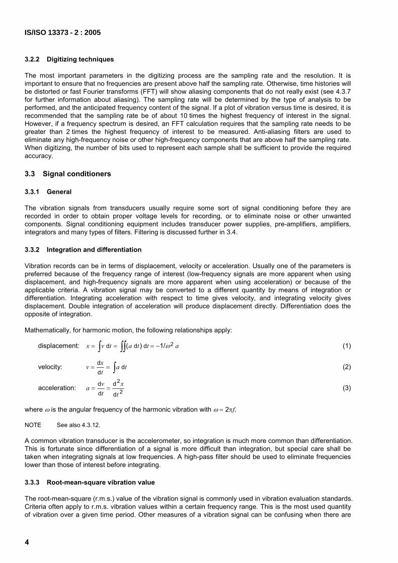
many frequency components, or when there is modulation, etc. However, the r.m.s. value is a mathematical quantity that can be found for any signal, and most instruments are designed to find that quantity (see Figure 5). Alternatively, the r.m.s. value may be found by using a spectrum analyser, by integrating the spectrum between the upper and lower frequencies of interest.

A vibration signal may be filtered as required and displayed on an r.m.s. meter if the reading does not change significantly in a short time period. However, if the indicated output varies significantly, an average over a certain period of time shall be obtained. This may be done with an instrument that has a longer time constant.

a) Sinusoidal signal where the r.m.s. value equals 0,707 times the peak value

b) Non-sinusoidal signal Key 1 peak value 2 r.m.s. value

Figure 5 — R.m.s. value

3.3.4 Dynamic range

The dynamic range is the ratio between the largest and smallest magnitude signals that a particular analyser can accommodate simultaneously. The magnitudes of the signals are proportional to the output voltages of the transducers, usually in millivolts.

The dynamic range in analog systems is usually limited by electrical noise. This is usually not a concern with respect to the transducer itself, but filters, amplifiers, recorders, etc., all add to the noise level, and the result may be surprisingly high.

In digital systems, the dynamic range is dependent on the sampling accuracy, and the sampling rate shall be adequate for the frequencies of concern. The relationship between the number of bits, N, used to sample an analog signal and the dynamic range D (if one bit is used for the sign) is as follows:

6 (N − 1) = D dB (4)

Therefore, a dynamic signal analyser (DSA) with 16 bits of resolution will have a dynamic range of 90 dB, but any inaccuracies will reduce the dynamic range.

3.3.5 Calibration

The calibration of individual transducers is well covered in the referenced documents (e.g. ISO 16063-21), and is usually carried out in the laboratory before their use in situ. It is recommended, however, that a calibration check be carried out for any field installation. The field calibration check normally does not include the calibration of the transducer, but does include the rest of the measuring/recording system, such as amplifiers,

IS/ISO 13373 - 2 : 2005

5

6

filters, integrators and recorders. Most often it involves the insertion of a known signal into the system to see what output relates to it. The signal may be a d.c. step, a sinusoid or random noise, depending on the type of measurement.

Certain transducers, such as displacement transducers or proximity probes, are precalibrated. However, in this case, their calibrations should be checked in the field in conjunction with the surface being measured, since proximity probes are sensitive to shaft metallurgy and finish. Calibration of these probes is carried out in place with micrometre spindles, and the outputs for each are noted.

When checking the calibration of seismic transducers in the field, a shake table is required.

Strain gauges are also often calibrated in the field after they are installed. The most desirable calibration is for a known load to be applied to the component being measured. If that is not practical, a shunt calibration may be made where a calibration resistor is connected in parallel with the strain gauge, thus changing the apparent resistance of the gauge by a known amount, which is equivalent to a certain strain determined by the gauge factor.

3.4 Filtering

There are three basic types of filters available for signal conditioning and analysis:

low pass,

high pass, and

bandpass.

Low-pass filters, as the name implies, are transparent only for the low-frequency components of the signal, and they block out the high-frequency components above the filter limiting frequency (cut-off frequency). Examples of application are anti-aliasing filters (see 4.3.7), or filters that exclude high-frequency components that are unwanted for special investigations (e.g. gear meshing components for balancing).

High-pass filters are mainly used to exclude low-frequency transducer noise (thermal noise), or some other unwanted components from the signal, prior to analysis. This can be important since such components, although of no interest, can dramatically reduce the useful dynamic range of the measurement equipment.

Bandpass filters, when included for analysis, are used to isolate distinct frequency bands. Very common bandpass filter types are the octave filters or 1/n octave filters, which are especially used to correlate vibration measurements with noise measurements.

Filtering is particularly important when analysing signals with large dynamic ranges. If there are frequencies in the spectra with both high and low amplitudes, for instance, they cannot usually be analysed with the same level of accuracy because of limitations in the dynamic range of the analyser. In such cases, it may be necessary to filter out the high-amplitude components to examine more closely those of low amplitude.

Filtering is also important for separation of informative signals and disturbances (as electronic noise is in the high-frequency range or seismic waves are in a very low-frequency range).

When filters are used to isolate a particular frequency component to examine the waveform, care shall be taken to ensure that the filter sufficiently excludes any component of frequencies other than those of interest. Simple filters, analog as well as digital, do not have very sharp cut-off characteristics, because the filter slope outside of the transmission band is poor.

EXAMPLE A particular filter with a 24 dB per octave slope will pass about 15 % of a component with twice the frequency, and about 45 % of a component with 1,5 times the cut-off frequency. To improve the filter’s suppression characteristics, several simple filters can be cascaded, or a higher-order filter can be used instead.

IS/ISO 13373 - 2 : 2005

4 Data processing and analysis

4.1 General

Data processing consists of raw-data acquisition, filtering out unwanted noise and/or other non-related signals, and formatting the measured signals in the form required for further diagnosis. Therefore, data processing is an important step towards achieving a fruitful and meaningful diagnosis. The device that acquires the vibration signals from the transducer should have adequate resolution in both amplitude and time. If digital data acquisition is utilized, then the amplitude resolution should be high enough for the application. A higher number of bits of resolution provide the ability to obtain greater accuracy and sensitivity, but it typically requires more expensive hardware and greater processing power.

Once the signals are acquired, the next step is to process them and then display the outputs in various useful formats so that the diagnosis is made much easier for the user. Examples of such formats include Nyquist plots, polar plots, Campbell diagrams, cascade and waterfall plots and amplitude decay plots. The objective of this clause, therefore, is to present these various methods of presentation available to the user in order to determine better the conditions of machines.

4.2 Time domain analysis

4.2.1 Time wave forms

In the past, waveform analysis was the primary method of vibration analysis. An instantaneous vibration versus time strip chart or oscillograph was usually analysed graphically, and broadband peaks were noted. While these broadband techniques are still being used, it is helpful to look at the waveform with some of the more basic techniques in mind. For example, a scratched journal can be detected by looking at waveform data from displacement transducers, a waveform with a clipped top or bottom can indicate a rub, mechanical looseness, etc.

While these time-domain signatures can portray waveforms that provide basic information regarding the nature of a phenomenon occurring in a machine, the more in-depth frequency analysis techniques described in 4.3 may be required.

The analysis of waveforms is based on the principle that any periodic record may be represented as a superposition of sinusoids having frequencies that are integral multiples of the frequency of the waveform. Figures 6 to 9 show several examples of waveforms.

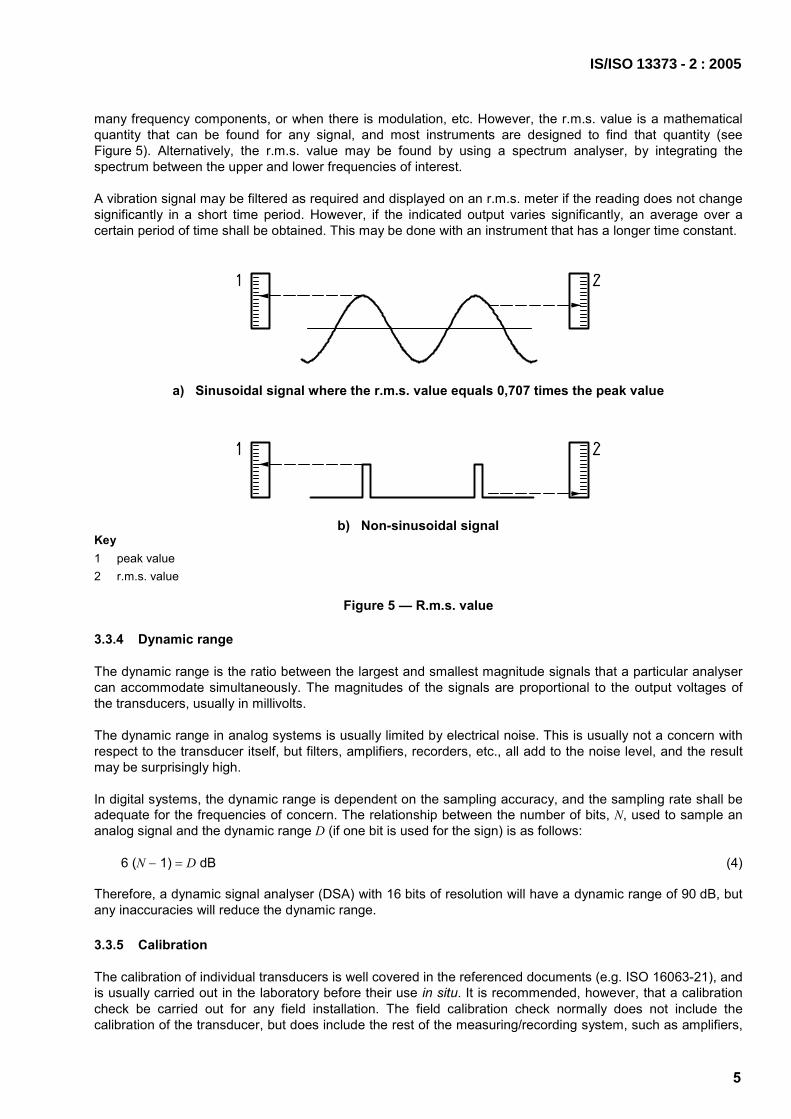
Figure 6 is essentially a one-cycle sinusoid with a constant amplitude. The double amplitude (or peak-to-peak) of the vibration is obtained by measuring the double amplitude of the trace, and multiplying by the sensitivity of the measuring and recording system, which is found by calibration. The frequency is found by counting the number of cycles in a known time period. The time on an oscillograph is indicated by timing lines, or simply by knowing the paper speed. For the trace shown, there are 60 timing lines per second; therefore, the 12 lines indicate that the fundamental period, T, is 0,2 s, and hence the frequency, f = 1/T, is 5 Hz. Accuracy is improved if the number of cycles in a longer section of the record is used.

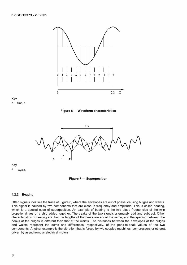
Figure 7 is the superposition of two sinusoids with three cycles of the lowest frequency shown. The components can be separated by drawing sinusoidal envelopes (upper and lower limits) through all the peaks and troughs as shown. The amplitude and frequency of the low-frequency component is that of the resulting envelope. The vertical distance between envelopes indicates the peak-to-peak value of the high-frequency component, and the high frequency can usually be counted. In this example, it can be found that the frequencies differ by a factor of three. When the frequency ratio of two superimposed sinusoids is high, they may be separated as shown; in all other cases a Fourier analysis is more useful.

IS/ISO 13373 - 2 : 2005

7

8

Key X time, s

Figure 6 — Waveform characteristics

Key a Cycle.

Figure 7 — Superposition

4.2.2 Beating

Often signals look like the trace of Figure 8, where the envelopes are out of phase, causing bulges and waists. This signal is caused by two components that are close in frequency and amplitude. This is called beating, which is a special case of superposition. An example of beating is the two blade frequencies of the twin propeller drives of a ship added together. The peaks of the two signals alternately add and subtract. Other characteristics of beating are that the lengths of the beats are about the same, and the spacing between the peaks at the bulges is different than that at the waists. The distances between the envelopes at the bulges and waists represent the sums and differences, respectively, of the peak-to-peak values of the two components. Another example is the vibration that is forced by two coupled machines (compressors or others), driven by asynchronous electrical motors.

IS/ISO 13373 - 2 : 2005

Key

X time, s Y amplitude

a Peak-to-peak value at waist: 0,2. b Peak-to-peak value at bulge: 0,7. c Waist. d Bulge. e Vibration cycle: 0,33 s corresponds to 3 Hz. f Beat cycle: 2 s corresponds to 0,5 Hz.

Figure 8 — Example of beating

EXAMPLE If the components’ amplitudes are Xm for the major and Xn for the minor, measurements show that Xm + Xn = 0,7 and Xm − Xn = 0,2, the solution being Xm = 0,45 and Xn = 0,25. These record amplitudes have to be multiplied by the system sensitivity to get actual amplitudes. The major frequency can be found by counting the number of peaks as described before (in Figure 8 it is 3 Hz). This frequency is also an integral multiple of the beat frequency, in this case 6 times. The frequency of the minor component is either one more (7) or one less (5) times the beat frequency. The spacing of the peaks at the waist indicates which one it is, since it reflects the major component. In Figure 8 the spacing is narrower so the major component has the higher frequency. In Figure 8, the beat frequency is 0,5 Hz and the minor frequency is 5 times that, i.e. 2,5 Hz.

It should be noted that the beat frequency is the difference between the frequencies of both components, but the average peak frequency is equal to one-half the sum of both. A simple rule for calculating the frequencies is:

fb = fm − fn (5)

where

fb is the beat frequency;

fm is the frequency of the major component;

fn is the frequency of the minor component.

In the example shown in Figure 8, by counting the peaks, there are 6 peaks in 2 s, which means fm = 3 Hz. The beat cycle is 1 cycle in that same time period, which means fb = 1/(2 s) = 0,5 Hz. Inversing Equation (5) to become fn = fm − fb, yields the frequency of the minor component fn = 3 Hz − 0,5 Hz = 2,5 Hz.

IS/ISO 13373 - 2 : 2005

9

10

4.2.3 Modulation

Figure 9 shows the trace of a modulated vibration signal. It looks similar to beating but there is actually only one component whose amplitude is varying with time (modulating). This is distinguishable from beating because the spacing of the peaks is the same at the bulges and the waists. Also, the length of the bulges may not be the same. Gear problems often result in modulation of the gear mesh frequency at the gear rotational frequency.

Unfortunately, many vibration records contain more than two components, and may involve modulation and perhaps beating as well. Such records are extremely difficult to analyse, but the analyst may be able to find sections of the record in which one component is temporarily dominant, and obtain the frequency and amplitude of that component in that section.

Figure 9 — Modulation

4.2.4 Envelope analysis

Envelope analysis is a process for the demodulation of low-level components in a narrow frequency band, which are obscured by a high-level broadband vibration (impulse-excited free vibration, gear meshing vibration, and others). Envelope detection provides a means for recognizing flaws earlier and with greater reliability. Its most common application is in analysis of gears and rolling element bearings where a low-frequency, generally low-amplitude repetitive event (such as a defective tooth entering mesh or a spalled ball or roller striking a race) excites high-frequency resonance(s), resulting in the high frequency being modulated by the defect frequency. A sample of an envelope trace is shown in Figure 10.

It should be noted that the modulated component needs to be separated previously by narrow band filtering.

Figure 10 — Envelope analysis

4.2.5 Monitoring of narrow-band frequency spectrum envelope

Monitoring of narrow-band frequency spectrum envelope detects any penetration of an envelope, which is usually an alarm limit, around a reference spectrum. The constant-bandwidth envelope, where the frequency difference is the same number of lines at low and high frequencies, is generally used for constant-speed machines.

A constant-percentage bandwidth envelope increases the frequency difference (offset) between the envelope and the monitored component proportionally to the increase in frequency. This method has advantages because all harmonic components will remain in the same frequency band over small speed changes.

IS/ISO 13373 - 2 : 2005

Amplitude limits for individual frequency components are of two types. A constant-percentage offset is the most commonly used because it is the simplest to calculate and only requires a single reference spectrum.

A more representative method is to calculate a statistical mean for each segment in the envelope, and then set the alarm limit 2,5 to 2,8 standard deviations above the mean. The statistical calculation requires 4 or 5 high-resolution spectra, and then automatically accounts for normal differences in amplitude variation commonly observed in the machinery spectra.

4.2.6 Shaft orbit

Orbit analysis can be performed on any machine using displacement transducers usually mounted 90° apart. On large rotating machinery with sleeve bearings, it is common practice to use shaft orbit analysis to determine the movement of the shaft within the bearing clearance space. However, care should be taken to ensure that the shaft orbit display is not distorted unnecessarily by the effects of shaft mechanical and electrical run-out. Proper interpretation of the orbit can yield insight into the nature of the forcing function. It is also possible to determine whether the rotor whirl is forwards (in the direction of rotation) or backwards (against the rotation). Orbit presentations are displayed as either unfiltered or filtered signals. Typical broadband (unfiltered) and single-frequency (filtered) orbit plots are shown in Figure 11.

a) Unfiltered b) Filtered

Figure 11 — Shaft orbits

The synchronous (1 ×) filtered display is common; however, other harmonics or sub-synchronous frequencies are displayed in an orbit presentation to further describe or solve a problem. A mark (point, highlight, etc.), which provides a shaft reference (e.g. once-per-revolution signal), gives information about the relationship between the vibrational and the rotational frequencies.

The orbit plot presents the dynamic motion of the centre of the rotating shaft at the measurement plane. An orbit is sometimes called a Lissajous presentation. The transducers for the orbits should be the same type and should be mounted orthogonally (90° apart). If the transducers are not orthogonal, the orbit will be skewed. In the case of a notched shaft, the convention is blank – bright. Blank indicates the beginning of the notch, bright indicates the end of the notch. Therefore, in Figure 11 the whirl direction is clockwise.

The direction of shaft rotation, clockwise or counter-clockwise, is independently determined depending upon the view direction. If the whirl direction is the same as the direction of rotation, the vibration is referred to as forward whirl. Backward whirl is when the whirl direction is opposite from the direction of rotation. In Figure 11, since both the rotation and the whirl directions are clockwise, the whirl is forward.

IS/ISO 13373 - 2 : 2005

11

12

4.2.7 D.c. shaft position

To determine the d.c. shaft position, displacement transducers are frequently used to give indications of the relative loading of sleeve bearings by their eccentricity ratios. The attitudes of the journals within their bearings as measured from the d.c. part of the signal (i.e. the gap) is very useful in monitoring large machines. The d.c. position can validate appropriate bearing lift and correct shaft position. Care should be taken, however, to avoid misrepresentation due to d.c. signal drift over a long period of time.

4.2.8 Transient vibration

Transient speed vibration is usually described as the vibration information obtained during the start-up and coast-down conditions of a machine train. The vibration data are usually displayed in presentation formats such as cascade (waterfall) diagrams, Bode plots, polar diagrams (Nyquist diagrams) and Campbell diagrams.

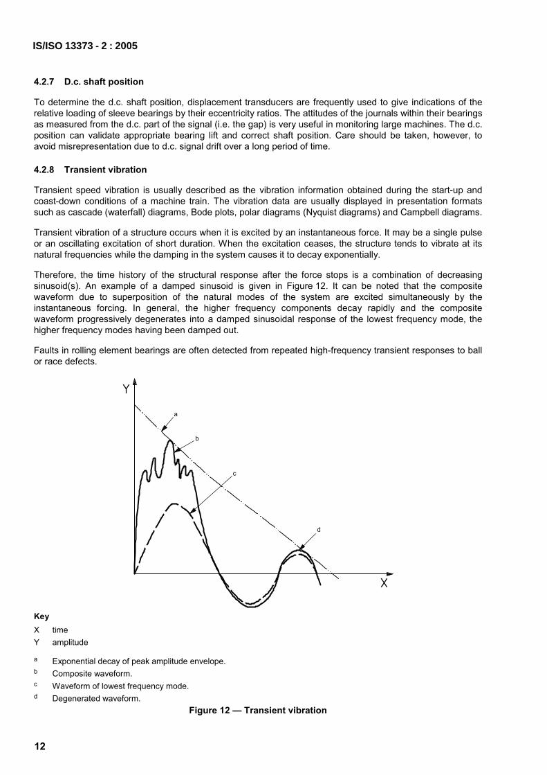
Transient vibration of a structure occurs when it is excited by an instantaneous force. It may be a single pulse or an oscillating excitation of short duration. When the excitation ceases, the structure tends to vibrate at its natural frequencies while the damping in the system causes it to decay exponentially.

Therefore, the time history of the structural response after the force stops is a combination of decreasing sinusoid(s). An example of a damped sinusoid is given in Figure 12. It can be noted that the composite waveform due to superposition of the natural modes of the system are excited simultaneously by the instantaneous forcing. In general, the higher frequency components decay rapidly and the composite waveform progressively degenerates into a damped sinusoidal response of the lowest frequency mode, the higher frequency modes having been damped out.

Faults in rolling element bearings are often detected from repeated high-frequency transient responses to ball or race defects.

Key X time Y amplitude

a Exponential decay of peak amplitude envelope. b Composite waveform. c Waveform of lowest frequency mode. d Degenerated waveform.

Figure 12 — Transient vibration

IS/ISO 13373 - 2 : 2005

4.2.9 Impulse

Impulse response is the time history of the vibratory response of a mechanical system to an impulse that can be represented as a force, F, applied over a very small period of time, ∆t, where the impulse is the integral of F1⋅dt from t to (t + ∆t), see Figure 13.

In many cases, impulse response is used to identify resonance frequencies in stationary structures.

Key

X time Y force

Figure 13 — Impulse excitation

4.2.10 Damping

Damping is the mechanism by which vibratory motion is converted to other forms of energy, usually heat, resulting in decaying vibration magnitudes. The amount of damping, c, is often proportional to the vibratory velocity and, even when it is not, it is often assumed to be for purposes of mathematical analysis. A system has critical damping, cc, if it has the smallest amount of damping required to return the system to its equilibrium position without oscillation. If the system’s damping is less than critical, it will oscillate with decaying amplitudes (see Figure 14 and ISO 2041). For a multi-degree-of-freedom system, some modes may have less than critical damping and some may have more.

Key X time Y amplitude

Figure 14 — Decaying amplitudes due to damping

IS/ISO 13373 - 2 : 2005

13

14

If the amplitude of the decaying vibration of a particular mode, X, is plotted versus the time duration, the logarithmic decrement, d, is:

d = 1/n ln(X1/Xn+1) (6)

where n is the number of cycles for the amplitude to decay from X1 to Xn+1.

The loss factor is a common measure of the relative damping in a system. The logarithmic decrement, d, is related to the loss factor, h, by h = d/π.

NOTE 1 Typically, the symbols used to denote the loss factor include h, z and η. Those for the logarithmic decrement include α and Λ.

The loss factor can also be found in terms of the decay rate, ,X ′ in decibels per second, as follows:

( )n/ 27,3h X f′= (7)

where fn is the natural frequency in hertz.

The amount of damping, c, in a system is indicated by Q, which is the magnification factor at the undamped natural frequency. The magnification factor is a function of frequency and is the ratio of the system’s dynamic displacement amplitude to the static displacement of the system if it were subjected to a constant force of the same magnitude. Provided that there is no significant interaction between the modes, then for a particular mode, Q may be found from:

Q = 1/(2c/cc) (8)

From measured response curves, Q may be approximated for a particular mode from the ratio of the resonant frequency, fr, to the difference between the frequencies at the half-power points (0,707 times the maximum amplitude) on each flank of the curve:

Q = rff∆

(9)

where

fr is the resonant frequency;

∆f = f2 − f1 with f1 and f2 being the half-power points.

The magnification factor is related to the logarithmic decrement by the following approximation:

Q ≈ π/d (10)

NOTE 2 If the damping is small, Q = 1/h.

As an example, Figure 15 shows a typical representation of the Q factor derived from a Bode plot. A similar result can be obtained from a polar diagram.

Damping is a useful quantity when investigating the cause and effect of vibration in rotating machinery. A mode near the operating speed may be acceptable as long as it is well damped and therefore not contributing to the response. Alternately, a mode with very little damping may be so sensitive that the machine will respond violently, or may not even be able to pass through a resonant speed.

4.2.11 Time domain averaging

Each signal contains components that are synchronous with processes or motions in the monitored machine or equipment, as well as non-synchronous ones (with an origin that is independent of the system under observation). These components can be separated by frequency analysis (see 4.3). Another common technique applied to identify these occurrences is called time domain averaging. In this process, each data

IS/ISO 13373 - 2 : 2005

sample is synchronized to different rotating elements via a reference pulse or a trigger. The averaging, which can range from a few samples to more than 200, is computed in the time domain, and a spectrum is obtained only based on the resulting averaged time waveform. Those time signal parts which are non-synchronous with the reference progressively cancel each other. The more averages the better, the number depends on the application.

In time domain averaging, the corresponding samples are actually algebraically added for each record, and then divided by the number of records. The result is that the desired repeating waveform remains intact while all other averages tend toward zero (including other repeating waveforms). The rate at which they decay away equals the square root of the number of averages.

NOTE 100 averages (records) will reduce the unwanted signals by a factor of ten; 10 000 averages will reduce them by a factor of 100.

Key X frequency Y response

Figure 15 — Q factor

This technique is very useful for the identification of which rotor in a multiple-rotor machine is the source of a vibration phenomenon. It may be used to detect various faults, such as damaged gears, blades and rolls in paper machines.

EXAMPLE 1 A good example is in the case of a turbine-driven pump with gear drive with different shaft speeds, where there is a once-per-revolution synchronizing trigger on each shaft. The signal from an accelerometer mounted on the gearbox may be analysed using time domain averaging in which the process is repeated for each synchronizing trigger. Using the turbine shaft trigger, the signal reduces to a sinusoidal waveform indicating the degree of unbalance in the turbine shaft. Using the pump shaft trigger, the signal reduces to a periodic pattern at vane passing frequency, indicating a fixed radial offset of the pump shaft within its housing.

EXAMPLE 2 Another example is where strain gauge bridges are mounted on two large hydroturbine blades, and their signals brought out by means of telemetry. A once-per-revolution trigger is used to synchronize the time domain averaging process. After several averages to reduce the flow noise, an uneven pattern may emerge which is identical for each blade, but offset in time by the rotational angle between the blades. The diagnosis is an uneven flow through the series of wicket gates that feed the turbine. The pattern is then used to re-adjust the gates to even out the flow and reduce the dynamic stresses on the blades.

IS/ISO 13373 - 2 : 2005

15

16

Although very effective, time domain averaging, by its very nature, cannot show asynchronous events such as antifriction bearing faults.

The averaging of complex frequency spectra of successive realizations normally requires a steady-state vibration condition. If there is an unsteady excitation frequency or a changing rotational speed, the simple time domain averaging does not apply. Instead of this, the signal needs to be sampled in constant intervals of the exciting process (e.g. equidistant rotor angle intervals or other positions; this can be done by means of an encoder). The result of the succeeding frequency transformation is an ordering spectrum instead of a frequency spectrum. For impulse response signals, averaging may be executed in the time domain by event triggering, e.g. a trigger tuned by the excitation impulse.

The source of the trigger is not limited to rotating equipment. Other applications, for instance, are paper machine belts, conveyor belts, etc. In addition, the source of the signal is not limited to vibration. It may be a process signal related to the machine in question that can identify a malfunction or a process parameter that should be monitored for fault development. A frequency multiplier may also be used instead of triggering from different shafts, e.g. in the case of multiple shafts such as in a gear box.

4.3 Frequency domain analysis

4.3.1 General

A great deal of vibration analysis is done in the frequency domain because the various sources of vibration can usually be isolated by the frequencies at which they occur. A single channel analysed in the frequency domain gives a great deal of information, but often it is important to relate vibration to a second channel as either a phase or amplitude reference, or both.

4.3.2 Fourier transform

The basic technique for converting a broadband time trace to discrete frequencies, or frequency bands, is by the application of the Fourier transform (FT), a mathematical technique that identifies the sinusoidal components that make up the total vibration signal, including any mechanical or electrical noise that may be present. This analysis can be realized with the help of a computer and signal processing software, by special devices (which are usually called a Fourier analyser), or by hardware microchips (DSPs). More commonly used in analysers now is a more efficient mathematical routine, the fast Fourier transform (FFT).

The time wave form of a vibration signal is converted into distinct sinusoidal components as a function of frequency by means of the FFT, as shown in Figure 16. There are several important basic factors to take into account when setting up an FFT analyser to convert a time wave form into a meaningful frequency spectrum. There is a relationship between the bandwidth of the frequency lines (or bins), the frequency span and the length of the time trace. In Figure 16, the bandwidth is 2 Hz, which is 100 frequency lines between 0 and 200. These parameters should be chosen to optimize the frequency range of interest.

Due to the effects of aliasing (see 4.3.7), higher frequency components can be falsely identified as lower frequency. Anti-aliasing filters should be used in order to avoid this possibility.

The result of a Fourier transform is a complex spectrum, which can be displayed as

amplitude and phase, or

real and imaginary part

of each frequency component.

From a practical viewpoint, the magnitude spectrum has more information; therefore, the phase spectrum is mostly ignored.

IS/ISO 13373 - 2 : 2005

Key X frequency, Hz Y amplitude

Figure 16 — Magnitude frequency spectrum

4.3.3 Leakage and windowing

When sampling a waveform, leakage can occur if the sample contains a non-integral number of cycles. The result is smearing of frequency domain peaks because the sample inaccurately represents the waveform from which it was taken. A window function reduces these errors by correcting for this leakage. The Hanning window does an acceptable job for sine waves that are periodic and non-periodic as time records. Although the Hanning window is most commonly used, there are other types of windows that are available and may be used to enhance the signal.

For transient events a Uniform (rectangular) window produces better results. The Hamming window gives a narrower spectral peak than the Hanning window at higher levels, in exchange for flaring skirts further down. The Blackman window, and its derivatives Blackman Exact and Blackman Harris, give a wider peak than the Hanning, but with even lower skirts. The Flat Top window can improve amplitude accuracy over the Hanning window at the expense of being able to resolve small signals that are closely spaced to large ones in the frequency domain. It gives the widest peak, with skirts equivalent to the Hanning, but the top of the peak is flattest for the most accurate level readings with changing frequencies. By correcting sampling bias, windows improve asynchronous waveform plots such as spectrum, cascade and waterfall. The Flat Top window can also be used for calibration.

NOTE Time domain windows for Fourier Transform analysis are described in ISO 18431-2.

4.3.4 Frequency resolution

The mathematics of an FFT requires that the frequency span of interest be divided into a finite number of sections, and the amplitude of vibration within each section is displayed as a vertical line, sometimes referred to as a “baseband” spectrum. The number of sections is referred to as the number of lines of resolution (LOR),

IS/ISO 13373 - 2 : 2005

17

18

NLOR. There may be more than one frequency component at frequencies within a single LOR bin, and the analyser includes this total energy and displays it as a single line at the centre frequency of the bin.

It is important to have a sufficient number of LOR to distinguish between closely spaced frequency components, and to use a frequency span that includes all frequencies of interest. Normally, at least 400 LOR are used, but many machines require finer resolution than that. The following relationship applies:

NLOR = fmax/B (11)

where

NLOR is the number of lines of resolution;

fmax is the maximum frequency of interest;

B is the bandwidth (line spacing).

As the relationship shows, for the same frequency range of interest, the finer the resolution, the smaller the bandwidth.

4.3.5 Record length

A single realization of the Fourier transform requires only a short record length, T, and the length of record required for an FFT is dependent on the bandwidth, B, as follows:

T = 1/B (12)

The length of record available may restrict the resolution. As an example, if a spectrum has a span of 100 Hz and a resolution of 400 lines, the bandwidth shall be 1/4 Hz, and the record length shall be at least 4 s. For the same resolution, if the span increases by a certain factor, the record length decreases by the same factor, and the bandwidth becomes wider by the same factor.

If a machine changes speed slightly during a test, it is important to have the bins wide enough to include each frequency component of interest in a single bin. In the case of a large change in the machine speed, the signal needs to be sampled at constant angular intervals and the succeeding ordering spectrum be processed (see 4.2.11 and 4.3.8).

4.3.6 Amplitude modulation (sidebands)

Amplitude modulation as it is seen in the time domain is shown in 4.2.3. An FFT of a modulating sine wave will show the sine wave’s frequency and sidebands on either side of that frequency, at a distance from it which is equal to the modulating frequency. If the modulation is itself a sine wave, the sidebands will be distinct and only one will appear on each side of the main frequency. This can occur with a gear mesh frequency when one of the gears is eccentric or worn. If the modulation is periodic, such as once per revolution, but not sinusoidal, there will be several distinct sidebands. If the modulation is not periodic, the sidebands will be smeared and indistinct.

The presence of sidebands can be very helpful in the detection of broken rotor bars in large induction motors by measuring the decibel down values. The decibel down, LD, is equal to 20 times the logarithm of the ratio of the rotor bar fault peak value to the line frequency value. Mathematically, this relationship is:

LD = 20 lg(l1/lref) dB (13)

where

l1 is the amplitude of the sideband;

lref is the amplitude at line frequency (50 Hz or 60 Hz).

IS/ISO 13373 - 2 : 2005

As shown in Figure 17, the spectrum for a motor with no problems consists of a clear peak at the line frequency and sidebands equally spaced on either side. The magnitude of the sidebands may be over 60 dB down from the magnitude of the line frequency (60 Hz in this case).

Key X frequency, Hz Y magnitude

Figure 17 — Motor with no problems

Figure 18 is the spectrum for a motor with a fault. In this case, there is a distinct peak at line frequency and elevated sidebands at the rotor bar fault frequencies.

Key X frequency, Hz Y magnitude

Figure 18 — Motor with a fault

IS/ISO 13373 - 2 : 2005

19

20

It can be noted that the structure of the sidebands in the frequency domain has the same information as the envelope spectrum in the time domain.

4.3.7 Aliasing

Aliasing is a false representation of a frequency that can result when the sampling rate of a digital analyser is too low to describe that frequency adequately. It is much the same as when a point on a disc appears fixed if the sampling frequency from a strobe is exactly coincident with the disc rotational frequency. However, if the frequencies are not exactly synchronized, the disc will appear to be rotating slowly. Similarly, if a sine wave is sampled too slowly, it will appear to be a lower frequency. This is eliminated by low-pass filtering the signal before sampling to ensure that it contains no frequency components above half the sampling frequency. This is clearly presented in Figure 19. By comparing the frequency of the high-frequency sine wave and the sampling interval, it can be shown that the sampling frequency is lower than one-half the signal frequency. Therefore, the dotted low-frequency signal will be analysed as an aliasing signal instead of the actually measured one. This is why the sampled amplitudes (the marked joint points in both curves) correspond to the measured high-frequency signal, as well as to the low-frequency aliasing signal.

When the sampling rate is set exactly at two times the maximum expected frequency, this is known as the Nyquist frequency. In practice, most sampling rates are set at greater than two times the maximum frequency (about 2,56 times) to allow for a low-pass filter without a sharp cut-off.

Digital analysers today use anti-aliasing filters that remove all frequencies above 40 % of the sampling rate, before the time data are sampled and converted to digital data; therefore, with most digital analysers, aliasing is no longer a problem. However, the analyst should confirm this before analysing the data.

Key X time Y excitation

a 3/rev excitation. b 13/rev excitation. c 3 and 13 excitation.

Figure 19 — Aliasing

IS/ISO 13373 - 2 : 2005

4.3.8 Synchronous sampling

Rather than sampling at a fixed rate with respect to time, an external signal may be used in many analysers to control the sampling rate. Normally, the sampling rate will be some multiple of the external signal frequency. This is most often used with rotating machinery, where a revolution marker is used to determine the sample rate. The sample rate would be greater than two times the highest-order vibration of interest. There are four major advantages to this procedure, as follows.

a) If the speed of the machine changes, most frequency components which are related to the rotational frequency (blade, vane, gear mesh, etc.) will stay in the same frequency bin, rather than spreading the energy over more than one bin.

b) All orders of vibration are in the centre of a frequency bin where its amplitude is measured more accurately.

c) It is possible to average the series of digitized measuring values without consideration of changes in the rotational speed.

d) All orders of vibration will maintain the same phase angle with respect to the external signal. This means that the spectra can be averaged vectorially, reinforcing the pertinent orders of vibration, but causing other signals not associated with that rotational speed, including most noise signals, to average to zero.

The result of the Fourier transform of a synchronously sampled signal is the ordering spectrum X(n). The order n = 1 corresponds with one vibration period per one rotor revolution.

It is noted that digital order tracking is an approach used in practice (see 4.6).

When performing synchronous averaging, care should also be taken to avoid averaging out any non-harmonic signals of significance (e.g. bearing instability).

4.3.9 Spectrum averaging

Depending on the component frequencies of the signal, a single FFT requires only a fraction of a second or a few seconds of record. However, a modulating signal may require a longer time period to establish a stable average amplitude. Therefore, averaging successive FFTs is a very important function of analysers. If only one channel is available, the absolute amplitudes in each bin are averaged without regard to the phase. Averaging of the complete spectrum (real and imaginary part) requires a synchronization of each successive spectrum by a process-dependent trigger signal.

There are other averaging techniques that may be applied, such as frequency domain averaging, but this technique quickly becomes very complicated and is therefore used only for special applications.

Many analysers do, however, perform exponential averaging, which weights the FFTs with an exponentially increasing function, thereby weighting the signal in favour of the most recently recorded data. This technique is often used for studies of transient vibration in which the amplitudes are exponentially decreasing.

Another type of averaging found on analysers is peak averaging. This finds the maximum amplitude during a given time period of all the FFTs in each of the frequency bins and displays those peaks. Note that each peak is the average amplitude within its own time record.

4.3.10 Logarithmic plots (with dB references)

With vibration records, there are usually many frequency components with greatly varying amplitudes. Many of the components with small amplitudes are important but, when plotted on a linear scale, can hardly be seen. A logarithmic plot, which compresses the large components and enlarges the small, shows all the significant components, as well as the level of noise present. The amplitude, X, is plotted as level, L, in decibels:

L = 20 lg(X/Xref) dB (14)

where Xref is a reference value.

IS/ISO 13373 - 2 : 2005

21

22

Sometimes the frequency axis is also displayed in a logarithmic scale for better recognition, or for separation of the low-frequency components. On the abscissa, the decibel unit is not used (see 4.7).

Differences in decibels are equivalent to ratios, examples of which are shown in Table 1.

Table 1 — Differences in decibels and equivalent ratios

Difference dB Ratio

0 1

6 2

20 10

26 20

40 100

60 1 000

Ratios smaller than one are reflected by negative decibel values, e.g. a ratio of 1/2 is −6 dB.

Reference values for logarithmic levels are specified in ISO 1683, except for displacement. For vibration analyses, the values given in Table 2 may be used.

Table 2 — Reference values for logarithmic levels

Quantity Reference value

Acceleration 10−6 m/s2

Velocity 10−9 m/s

Displacement 10−12 m

Power 10−12 W

4.3.11 Zoom analysis

Often frequency components are too close together to distinguish between them on a normal FFT, which generally consists of 400 lines (base band); however others exist. Some analysers have higher resolution, but often zoom spectra are used to get better resolution. A zoom analysis creates a spectrum with a frequency scale that does not start at zero but at another free eligible frequency, so that the selected number of lines are utilized to expand the frequency range of interest. The bandwidth is correspondingly narrower; however, the record length will still be related to the bandwidth. One problem in using the zoom spectra is that the frequencies must be more stable because of the narrower bandwidth.

An example of the use of zoom spectra is in gear fault analysis. When applied, a fault will result in sidebands of the gear mesh frequency and the spacing of the sidebands will indicate the faulted wheel. A similar zoom approach may also be useful to identify faults in rolling element bearings. Figure 20 shows the advantages of performing zoom analysis. Note that the frequency components not visible in the original zoomed spectrum are now visible.

IS/ISO 13373 - 2 : 2005

Key a Section of original spectrum. b Higher resolution translated spectrum.

Figure 20 — Zoom analysis

4.3.12 Differentiation and integration

Differentiation and integration are important in vibration analysis when signals shall be converted between displacement, velocity and acceleration. For rotating machinery, the vibration signal is often dominated by the synchronous component, and can therefore be harmonic motion. The following formulae then take on the following appearance in the time domain (see also 3.3.2):

displacement: ˆ sinx x tω= ⋅ (15)

velocity: ˆ ˆcos cosv x t v tω ω ω= ⋅ = ⋅ (16)

acceleration: 2 ˆ ˆ ˆsin sin sina x t v t a tω ω ω ω ω= − ⋅ = − ⋅ = − ⋅ (17)

and

acceleration: ˆ sina a tω= ⋅ (18)

velocity: ˆ ˆcos cosav t v tω ωω

= − ⋅ = − ⋅ (19)

displacement: 2ˆ ˆ ˆsin sin sina vx t t x tω ω ω

ωω= − ⋅ = − ⋅ = − ⋅ (20)

The displacement lags the velocity by 90°, and the velocity lags the acceleration by 90°. To convert between quantities in the frequency domain, both differentiation and integration may be carried out by dividing or multiplying, respectively, each component by its angular frequency. Most analysers include these functions for the frequency domain.

It is stressed that to utilize accurately the integration and differentiation formulae, the vibration signal must be predominantly synchronous. It is necessary to check to determine if the 1 × component is greater than 90 % of the unfiltered, or direct, component. Otherwise, each spectral frequency shall be converted separately.

IS/ISO 13373 - 2 : 2005

23

24

4.4 Display of results during operational changes

4.4.1 Amplitude and phase (Bode plot)

When a harmonic vibration signal is expressed in terms of an amplitude and phase, a second signal is required as a reference for the phase. It may be a shaft revolution marker, the vibration at a different location or direction, a measured force or some other appropriate reference. The frequency(ies) of the second signal shall be considered in relation to the frequencies of interest. For example, a shaft revolution marker could be used as a phase reference for rotational frequency or any of the higher harmonics of rotational frequency.

The phase may be expressed as between 0 and 360°, or ± 180°.

When the two signals represent different quantities (e.g. force, velocity, acceleration), care shall be taken to interpret the physical significance properly. Note that, for any sine wave, the displacement lags the velocity by 90°, and the velocity lags the acceleration by 90°. Very often, signal-conditioning equipment changes the phases of the signals, and differences between channels shall be compensated for.

The amplitude and phase of a sine wave may be plotted as a function of time. However, when the amplitude and phase of a machine vibration is plotted against the machine speed, it becomes a Bode plot, as shown in Figure 21.

Key X speed Y amplitude Y′ phase, degrees

a Resonance.

Figure 21 — Amplitude and phase (Bode plot)

4.4.2 Polar diagram (Nyquist diagram)

In a polar diagram, each point represents an amplitude/phase vector for a discrete frequency as shown in Figure 22. If the diagram includes several vectors for different rotating speeds, or other parameters, by showing only the connecting line between their tips, it is known as a Nyquist diagram.

A polar diagram shall have a phase reference, such as a shaft revolution marker, that indicates each 360° rotation of the shaft. Polar diagram (and/or Bode plots) are used to identify accurately the location (speed) of any resonances of the rotor/bearing/support system.

IS/ISO 13373 - 2 : 2005

NOTE The parameter is the rotor speed (r/min).

Figure 22 — Polar diagram (Nyquist diagram)

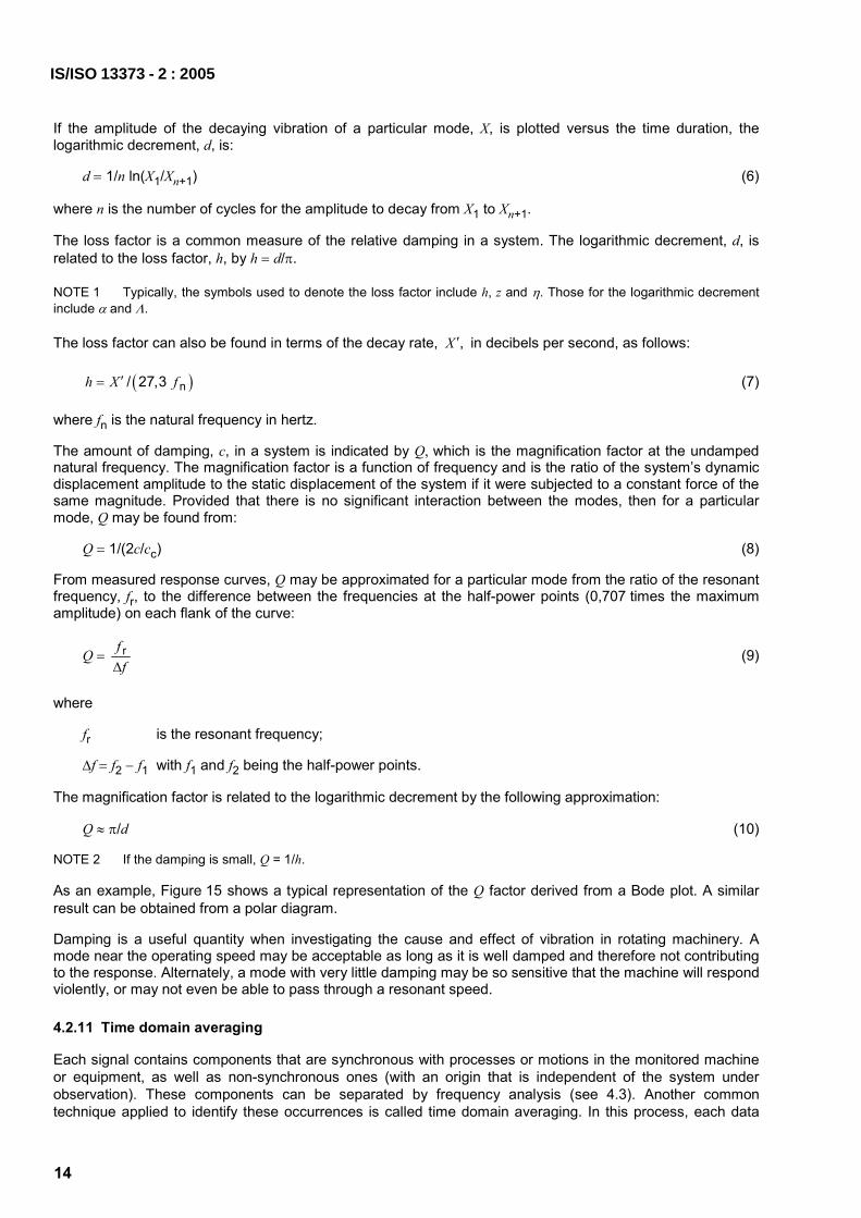
4.4.3 Cascade (waterfall) diagram

The cascade or waterfall diagram provides a simple comparison of several frequency analyses. It is a three-dimensional form of spectra display that clearly shows vibration signal changes related to another parameter (such as speed, load, temperature, time) taken for specified parameter values, such as time.

The sample cascade spectrum of Figure 23 is an overall picture of many vibration spectra for a machine in the start-up/coast-down region. Normally, the cascade spectrum display provides frequency (Hz or orders) versus machine rotational speed and vibration amplitude of the discrete frequency components. In some cases, however, the machine speed may be substituted by another variable (e.g. time, load), in which case it is then called a waterfall diagram. When using machine speed for this display, it is necessary to record a rotor speed/phase reference signal.

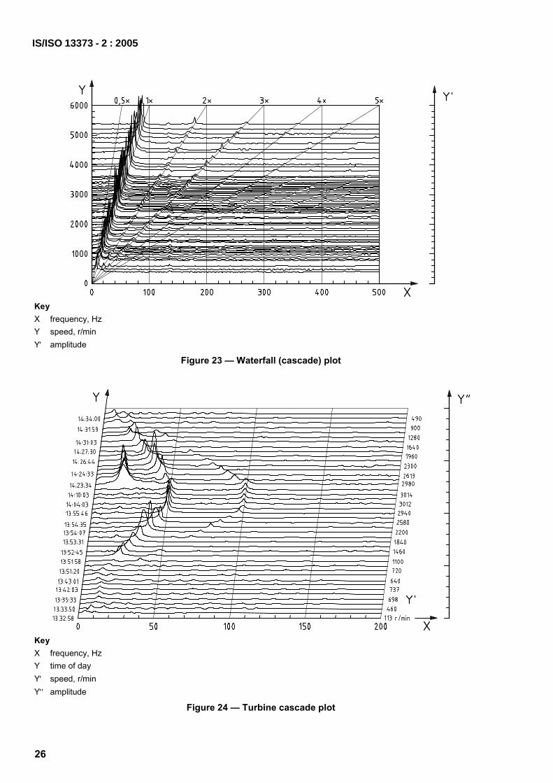
The cascade spectrum of Figure 24 shows the fundamental rotor speed (1 ×) and any other significant harmonic. It also shows the presence of rotor critical speeds, if in the transient speed range.

IS/ISO 13373 - 2 : 2005

25

26

Key X frequency, Hz Y speed, r/min Y′ amplitude

Figure 23 — Waterfall (cascade) plot

Key X frequency, Hz Y time of day Y′ speed, r/min Y′′ amplitude

Figure 24 — Turbine cascade plot

IS/ISO 13373 - 2 : 2005

The shape of the plot will vary, depending on the type of machine and the operation. For example, Figure 24 is a cascade plot of a 3 000 r/min (50 Hz) steam turbine during start-up and coast-down.

For time-dependent spectra, an alternative representation is to use a spectrogram. This is a two-dimensional presentation of a cascade plot which shows speed changes over time but indicates the amplitude height by different colours or intensitives of grey shading (see Figure 25).

NOTE The example in Figure 25 shows another machine than that in Figures 23 and 24.

Key X frequency, Hz Y time, s Y′ amplitude, m/s2 (indicated by grey shading)

Figure 25 — Two-dimensional spectrogram

4.4.4 Campbell diagram

The Campbell diagram (see Figure 26) is a special kind of cascade diagram. It relates the actual frequencies of individual frequency components, such as blade, vane, gear mesh, to the rotational speed. Vibration amplitude can be plotted in the third dimension, so it is represented by the height of the corresponding bars. Campbell diagrams are especially useful for identifying self-excited natural vibration.

IS/ISO 13373 - 2 : 2005

27

28

Key X speed, r/min Y frequency, Hz

a 1st speed harmonic. b 2nd speed harmonic. c Amplitude. d Natural frequency.

e Resonance speed. f Resonance speed. g Limit speed of instability. h Sub-synchronous vibration arising from rotor instability.

Figure 26 — Campbell diagram

4.5 Real-time analysis and real-time bandwidth

Real-time analysis refers to an analysis in which the results are displayed as the measurement is being made. It often simply means that data are displayed as they are recorded for the test engineer to observe. However, in this subclause, it relates to the time involved in acquiring data as opposed to processing it. If it takes longer to process a block of data than to acquire it, not all of the data can be processed as the data are being acquired, and it is not real-time analysis. It may be necessary to record a signal and then play it back, sometimes repeatedly, in order to analyse it. On the other hand, the data acquired over and above the amount processed may just be skipped (i.e. not processed).

In analog systems, a common type of real-time analyser consists of a bank of filters which can display all of the outputs simultaneously. Early octave or one-third-octave analysers were of this type.

In digital systems, the vibration signal is sampled to obtain successive time records, and each record is processed to obtain spectra or other characteristics. The sampling of the time record shall be complete before the processing of that record starts. However, sampling of one record and processing of the previous record can be done simultaneously. If it takes longer to sample a time record than it does to process the previous time record, all of the signal is analysed, and the analysis is considered real-time. If the processing takes

IS/ISO 13373 - 2 : 2005

longer than the sampling, parts of the signal are missed and the analysis is not considered real-time. Different analysers process data at different speeds, and the maximum frequency span at which data are processed real-time is the real-time bandwidth.

For most machinery measurements at a constant speed, real-time analysis is not required. However, for transient events, including start-ups and coast-downs, a real-time bandwidth that is too small may result in missing relevant data. The most common technique to avoid this is to record the entire event and then play it back at a lower speed to analyse it.

4.6 Order tracking (analog and digital)

When obtaining frequency spectra from machines, if the speed of the machine varies, it may be difficult to obtain meaningful averages because the energy from a particular order may be reflected in more than one frequency bin, and at lower levels than if the speed were constant. By controlling the sampling rate according to the speed of the machine by means of external sampling (see 4.3.8), all of the energy in a particular order of vibration will be reflected in just one frequency bin. This is normally accomplished by using a once-per-revolution signal as input to a dynamic signal analyser and is called order tracking.

Order tracking was first done with a tracking filter for alias protection, and a ratio synthesizer to change the r/min signal to a sampling frequency (2,56 times the highest order of interest). Noise and accuracy concerns, along with restrictions on the rates of change in r/min, led to computed order tracking, which digitizes the process.

In computed order tracking, both the vibration signal and the r/min signal are digitized with fixed sampling rates. The r/min signal is used to establish the sampling rate for each revolution, and the vibration signal is interpolated and re-sampled at the appropriate intervals for the order analysis to establish a stepwise changing individual sampling frequency for each revolution or, by means of polynomial interpolation, a continuously changing sampling frequency can also be generated.

As indicated in 4.3.8, this process has two additional advantages over time-based sampling. All the energy for each order is in the middle of the window for each bin, eliminating the error caused by not being in the middle, which can be up to 15 %.

The other advantage is that it is possible to obtain averaged records with the rotational angle a “time-axis” now, and also in the case of non-steady rotational frequency, and then to process ordering spectra for only the vibration at orders of the r/min. If vector averages are used, vibration at other frequencies will not have a constant phase with respect to the r/min, and will average to zero. Ordering spectra can be averaged without any smearing of the components.

4.7 Octave and fractional-octave analysis

An octave is another relative term signifying a doubled or halved frequency, depending on whether the frequency is being increased or decreased. For example, one octave above 100 Hz would be 200 Hz, while one octave below 100 Hz would be 50 Hz. Thus, while the decibel is a convenient unit to express amplitude ratios, the octave is a convenient way to express frequency ratios. For improved resolution, octaves can be logarithmically split into fractional octaves (e.g. one-third octaves).

4.8 Cepstrum analysis

The cepstrum analysis technique is the reverse transformation of the logarithmic-arithmetic power spectrum of measured vibration data in the time domain. A cepstrum is displayed in a spectral format with amplitude on the vertical axis and a pseudo time called “quefrency” on the horizontal axis. A cepstrum is a spectrum of a spectrum. A fundamental and its harmonic series are thus reduced to a single component.

A cepstrum is ideally suited to the analysis of complex signals containing multiple harmonic series such as generated by gearboxes or rolling element bearings. The ability to isolate and enhance periodic functions so their relationship can be identified is the major advantage of a cepstrum. See Table 3 for the step-by-step progression in the development of a cepstrum analysis.

IS/ISO 13373 - 2 : 2005

29

30

Table 3 — Processing of cepstrum

Activity Result

Measurement of the time history digitized signal x(t)

FFT of the digitized signal amplitude spectrum X(f)

Square the magnitudes of the components of the amplitude spectrum

power spectrum SXX(f) = X2(f)

Calculate 10 times the logarithm of the power spectrum

10 lg SXX(f) dB

Inverse FFT of 10 lg SXX(f) dB power cepstrum CXX(t)

IS/ISO 13373 - 2 : 2005

5 Other techniques

This part of ISO 13373 presents the most commonly used techniques when carrying out narrowband vibration condition monitoring and vibration diagnostics. However, there are other procedures that when applied to special cases can be very useful for solving particular problems. Some of these advanced techniques are listed below for information:

crest factor,

time history,

auto-correlation function,

cross-correlation function,

kurtosis,

composite or full spectra,

inverse Fourier transform,

high-frequency detection,

intensity methods,

multi-trend analysis (r.m.s. values, frequency components, hours, calendar time, high speed),

peak view analysis,

shock pulse measurements,

wavelets,

vector analysis, and

spike energy.

IS/ISO 13373 - 2 : 2005

31

32

Bibliography

[1] ISO 2041, Vibration and shock — Vocabulary

[2] ISO 2954, Mechanical vibration of rotating and reciprocating machinery — Requirements for instruments for measuring vibration severity

[3] ISO 5348, Mechanical vibration and shock — Mechanical mounting of accelerometers

[4] ISO 7919 (all parts), Mechanical vibration — Evaluation of machine vibration by measurements on rotating shafts

[5] ISO 10816 (all parts), Mechanical vibration — Evaluation of machine vibration by measurements on non- rotating parts

[6] ISO 10817-1, Rotating shaft vibration measuring systems — Part 1: Relative and absolute sensing of radial vibration

[7] ISO 13372, Condition monitoring and diagnostics of machines — Vocabulary

[8] ISO 13373-1, Condition monitoring and diagnostics of machines — Vibration condition monitoring — Part 1: General procedures

[9] ISO 16063-21, Methods for the calibration of vibration and shock transducers — Part 21: Vibration calibration by comparison to a reference transducer

[10] ISO 18431 (all parts), Mechanical vibration and shock — Signal processing

[11] VDI 3839 Blatt 1, Hinweise zur Messung und Interpretation der Schwingungen von Maschinen — Allgemeine Grundlagen (Instructions on measuring and interpreting the vibrations of machine — General principles) (Bilingual edition)

[12] VDI 3841, Schwingungsüberwachung von Maschinen — Erforderliche Messungen (Vibration monitoring of machinery — Necessary measurements) (Bilingual edition)

[13] MITCHELL, J. S. An introduction to machinery analysis and monitoring. Pennwell Publishing, 1993

IS/ISO 13373 - 2 : 2005

Bureau of Indian Standards

BIS is a statutory institution established under the Bureau of Indian Standards Act, 1986 to promoteharmonious development of the activities of standardization, marking and quality certification of goodsand attending to connected matters in the country.

Copyright

BIS has the copyright of all its publications. No part of these publications may be reproduced in any formwithout the prior permission in writing of BIS. This does not preclude the free use, in course of imple-menting the standard, of necessary details, such as symbols and sizes, type or grade designations.Enquiries relating to copyright be addressed to the Director (Publications), BIS.

Review of Indian Standards

Amendments are issued to standards as the need arises on the basis of comments. Standards are alsoreviewed periodically; a standard along with amendments is reaffirmed when such review indicates thatno changes are needed; if the review indicates that changes are needed, it is taken up for revision. Usersof Indian Standards should ascertain that they are in possession of the latest amendments or edition byreferring to the latest issue of ‘BIS Catalogue’ and ‘Standards: Monthly Additions’.

This Indian Standard has been developed from Doc No. : MED 28 (1013).

Amendments Issued Since Publication______________________________________________________________________________________

Amendment No. Date of Issue Text Affected______________________________________________________________________________________

______________________________________________________________________________________

______________________________________________________________________________________

______________________________________________________________________________________

______________________________________________________________________________________

BUREAU OF INDIAN STANDARDSHeadquarters:

Manak Bhavan, 9 Bahadur Shah Zafar Marg, New Delhi 110002Telephones: 2323 0131, 2323 3375, 2323 9402 Website: www.bis.org.in

Regional Offices: Telephones

Central : Manak Bhavan, 9 Bahadur Shah Zafar Marg 2323 7617NEW DELHI 110002 2323 3841

Eastern : 1/14, C.I.T. Scheme VII M, V.I.P. Road, Kankurgachi 2337 8499, 2337 8561KOLKATA 700054 2337 8626, 2337 9120

Northern : SCO 335-336, Sector 34-A, CHANDIGARH 160022 260 3843260 9285

Southern : C.I.T. Campus, IV Cross Road, CHENNAI 600113 2254 1216, 2254 14422254 2519, 2254 2315

Western : Manakalaya, E9 MIDC, Marol, Andheri (East) 2832 9295, 2832 7858MUMBAI 400093 2832 7891, 2832 7892

Branches: AHMEDABAD. BANGALORE. BHOPAL. BHUBANESHWAR. COIMBATORE. DEHRADUN.FARIDABAD. GHAZIABAD. GUWAHATI. HYDERABAD. JAIPUR. KANPUR. LUCKNOW.NAGPUR. PARWANOO. PATNA. PUNE. RAJKOT. THIRUVANATHAPURAM. VISAKHAPATNAM.

K.G. Computers, Ashok Vihar, Delhi

{{

{{{