ISE 754: Logistics Engineering

Michael G. KaySpring 2018

Topics1. Introduction2. Facility location3. Freight transport

– Exam 1 (take home)

4. Network models5. Routing

– Exam 2 (take home)

6. Warehousing– Final project– Final exam (in class)

Inside the box

Outsid

e the bo

x

2

Scope• Strategic (years)

– Network design

• Tactical (weeks‐year)– Multi‐echelon, multi‐period, multi‐product production and inventory models

• Operational (minutes‐week)– Vehicle routing

3

Strategic: Network Design

-120 -110 -100 -90 -80 -7015

20

25

30

35

40

45

50

1

2

3

4

5

Optimal locations for five DCs serving 877 customers throughout the U.S.

4

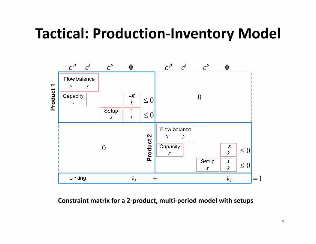
Tactical: Production‐Inventory Model

5

pc ic

0

0

sc 0

0

0

pc ic sc 0

1k 2k 1

0

0

Prod

uct 1

Prod

uct 2

Constraint matrix for a 2‐product, multi‐period model with setups

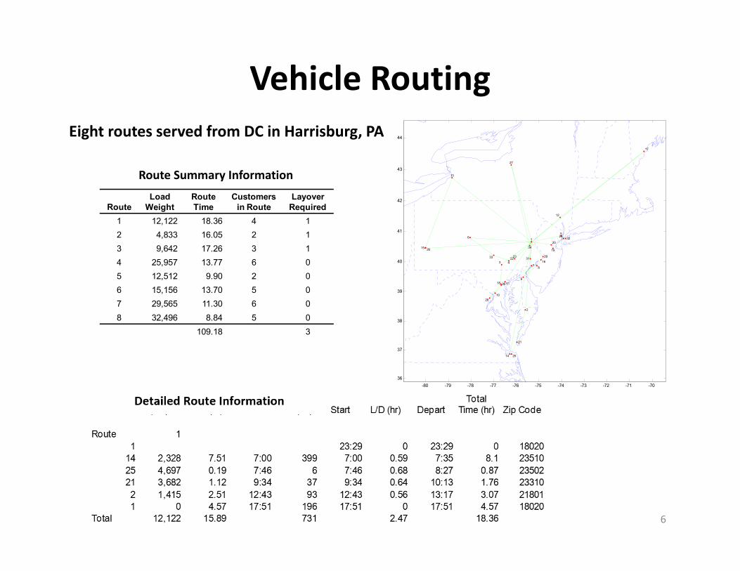
Vehicle RoutingEight routes served from DC in Harrisburg, PA

6

-80 -79 -78 -77 -76 -75 -74 -73 -72 -71 -7036

37

38

39

40

41

42

43

44

1

2

3 4

56

7 8

9

10

11

12

13

14

15

16

17

18

19

20

21

22 23

24

25

26

27

28

29

30

31

32

33

34

RouteLoad

WeightRoute Time

Customers in Route

Layover Required

1 12,122 18.36 4 12 4,833 16.05 2 13 9,642 17.26 3 14 25,957 13.77 6 05 12,512 9.90 2 06 15,156 13.70 5 07 29,565 11.30 6 08 32,496 8.84 5 0

109.18 3

Route Summary Information

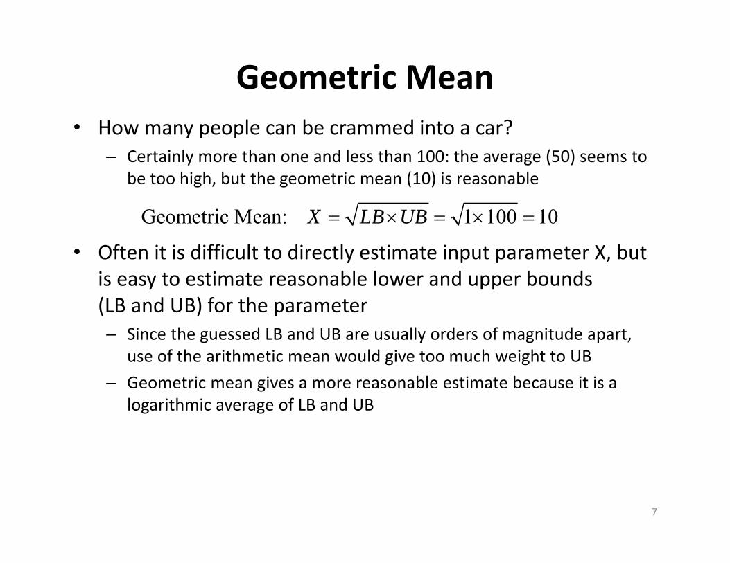
Geometric Mean• How many people can be crammed into a car?

– Certainly more than one and less than 100: the average (50) seems to be too high, but the geometric mean (10) is reasonable

• Often it is difficult to directly estimate input parameter X, but is easy to estimate reasonable lower and upper bounds (LB and UB) for the parameter– Since the guessed LB and UB are usually orders of magnitude apart, 

use of the arithmetic mean would give too much weight to UB– Geometric mean gives a more reasonable estimate because it is a 

logarithmic average of LB and UB

7

Geometric Mean: 1 100 10X LB UB

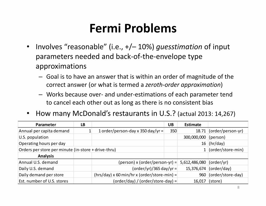
Fermi Problems• Involves “reasonable” (i.e., +/– 10%) guesstimation of input 

parameters needed and back‐of‐the‐envelope type approximations– Goal is to have an answer that is within an order of magnitude of the 

correct answer (or what is termed a zeroth‐order approximation)– Works because over‐ and under‐estimations of each parameter tend 

to cancel each other out as long as there is no consistent bias

• How many McDonald’s restaurants in U.S.? (actual 2013: 14,267)Parameter LB UB Estimate

Annual per capita demand 1 1 order/person‐day x 350 day/yr = 350 18.71                   (order/person‐yr)U.S. population 300,000,000      (person)Operating hours per day  16                         (hr/day)Orders per store per minute (in‐store + drive‐thru) 1                           (order/store‐min)

AnalysisAnnual U.S. demand (person) x (order/person‐yr) = 5,612,486,080  (order/yr)Daily U.S. demand (order/yr)/365 day/yr = 15,376,674        (order/day)Daily demand per store (hrs/day) x 60 min/hr x (order/store‐min) = 960                      (order/store‐day)Est. number of U.S. stores (order/day) / (order/store‐day) = 16,017                (store)

8

System Performance Estimation• Often easy to estimate performance of a new system if can assume either perfect or no control

• Example: estimate waiting time for a bus– 8 min. avg. time (aka “headway”) between buses– Customers arrive at random

• assuming no web‐based bus tracking

– Perfect control (LB): wait time = half of headway– No control (practical UB): wait time = headway

• assuming buses arrive at random (Poisson process) 

– Bad control can result in higher values than no control9

8Estimated wait time 8 5.67 min2

LB UB

http://www.nextbuzz.gatech.edu/

10

Crowdsourcing• Obtain otherwise hard to get information from a large group of online workers

• Amazon’s Mechanical Turk is best known– Jobs posted as HITs (Human Information Tasks) that typically pay $1‐2 per hour

– Main use has been in machine learning to create tagged data sets for training purposes

– Has been used in logistics engineering to estimate the percentage homes in U.S. that have sidewalks (sidewalk deliveries by Starship robots)

11

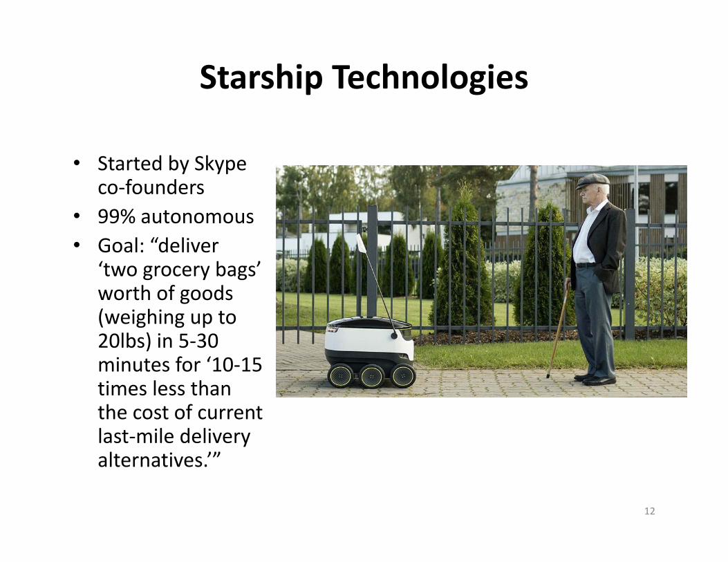
Starship Technologies

• Started by Skype co‐founders

• 99% autonomous• Goal: “deliver 

‘two grocery bags’ worth of goods (weighing up to 20lbs) in 5‐30 minutes for ‘10‐15 times less than the cost of current last‐mile delivery alternatives.’”

12

Matrix Multiplication

13

m n n p m p

Arrays must have sameinner dimensions

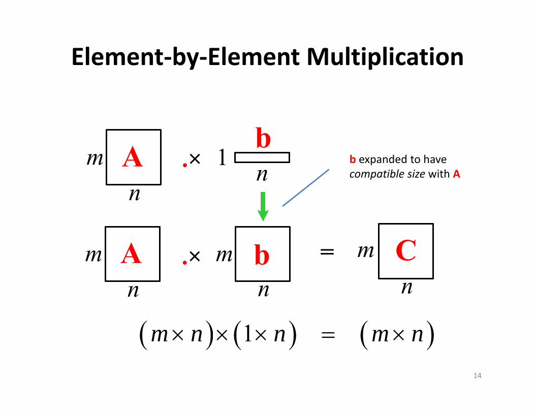
Element‐by‐Element Multiplication

14

b expanded to have compatible size with A

1m n n m n

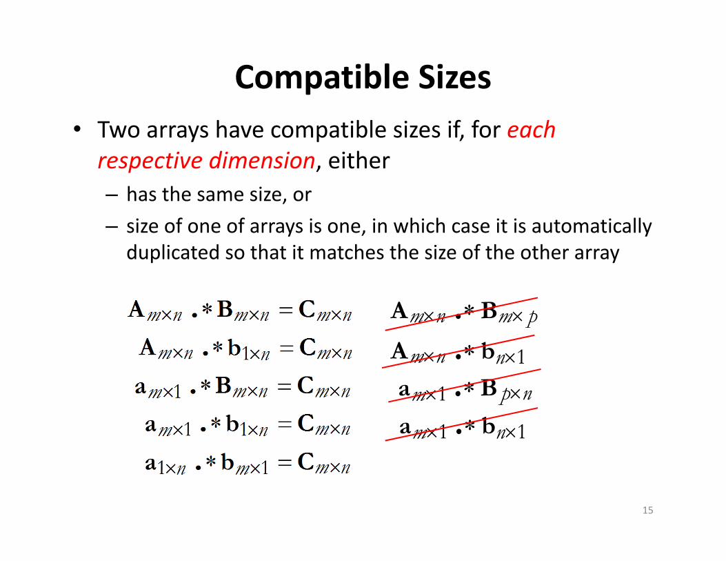
Compatible Sizes• Two arrays have compatible sizes if, for each respective dimension, either– has the same size, or – size of one of arrays is one, in which case it is automatically duplicated so that it matches the size of the other array

15

.m n m pA B

1.m n nA b

1 1.m na b 1 . p nma B

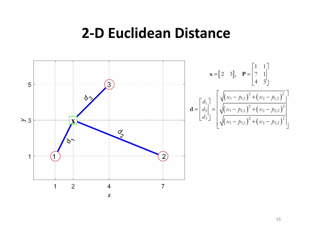
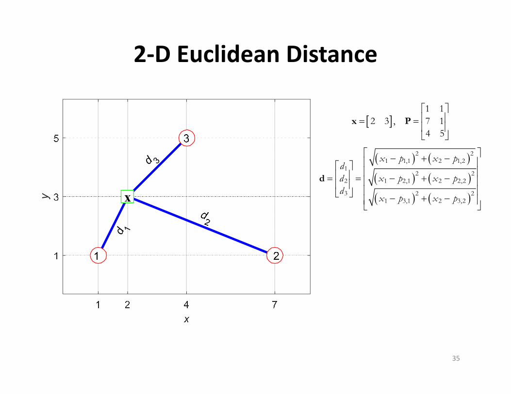
2‐D Euclidean Distance

2 21 1,1 2 1,2

12 2

2 1 2,1 2 2,2

3 2 21 3,1 2 3,2

1 12 3 , 7 1

4 5

x p x pdd x p x pd

x p x p

x P

d

y

d 1

d 316

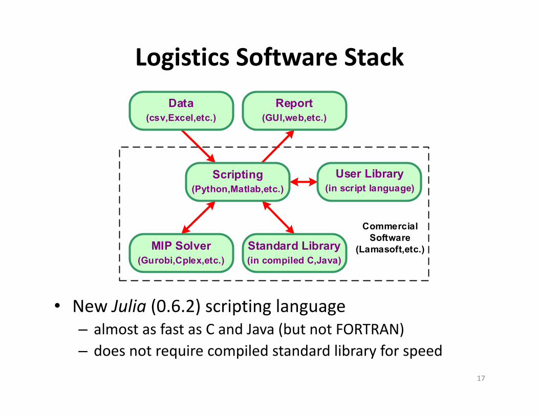
Logistics Software Stack

17

• New Julia (0.6.2) scripting language– almost as fast as C and Java (but not FORTRAN)– does not require compiled standard library for speed

MIP Solver(Gurobi,Cplex,etc.)

Standard Library(in compiled C,Java)

User Library(in script language)

MIP Solver(Gurobi, etc.)

Standard Library(C,Java)

Data(csv,Excel,etc.)

Report(GUI,web,etc.)

CommercialSoftware

(Lamasoft,etc.)

Scripting(Python,Matlab,etc.)

Basic Matlab Workflow• Given problem to solve:

1. Test critical steps at Command Window2. Copy working critical steps to a cell (&&) in script file (myscript.m) along 

with supporting code (can copy selected lines from Command History)– Repeat using new cells for additional problems

• Once all problems solved, report using:– >> diary hw1soln.txt– Evaluate each cell in script:

• To see code + results: select text then Evaluate Selection on mouse menu (or F9)• To see results: position cursor in cell then Evaluate Current Section (Cntl+Enter)

– >> diary off• Can also report using Publish (see Matlab menu) as html or Word• Submit all files created, which may include additional

– Data files (myscript.mat) or spreadsheet files (myexcel.xlsx)– Function files (myfun.m) that can allow use to re‐use same code used in 

multiple problems• All code inside function isolated from other code except for inputs/outputs:[out1,out2] = myfun(input1,input2)

18

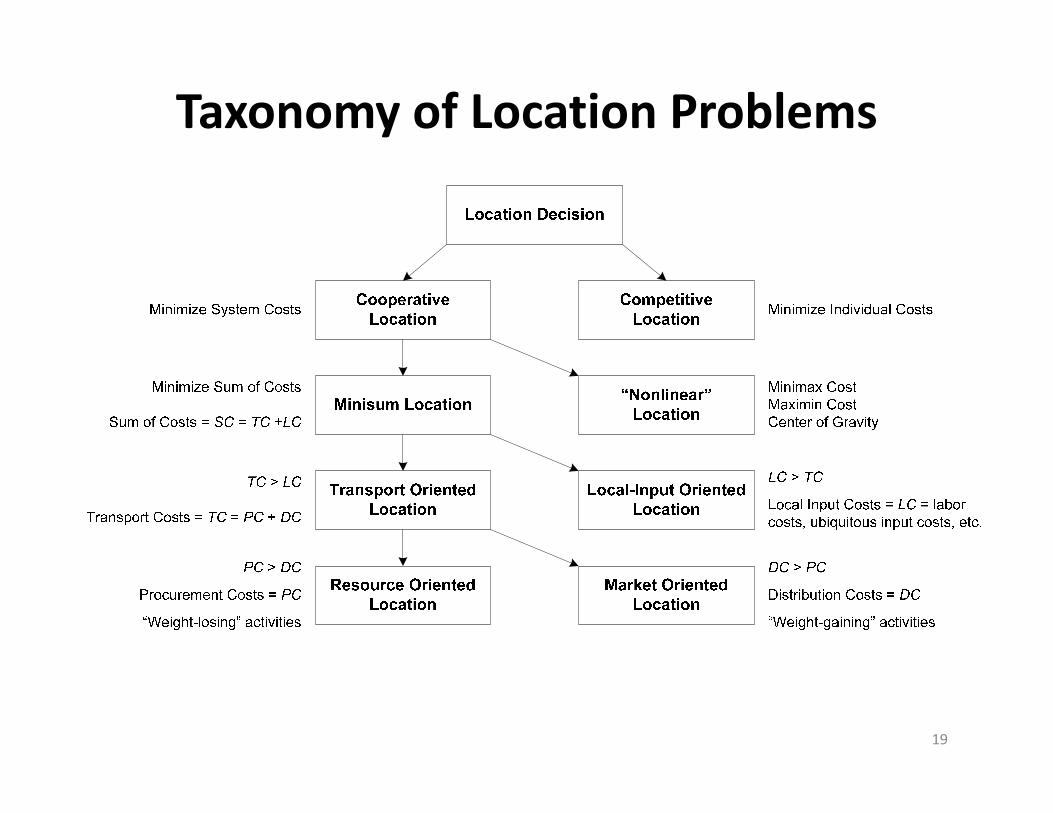
Taxonomy of Location Problems

19

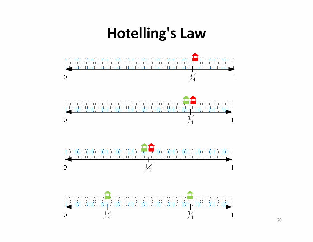
Hotelling's Law

34

34

12

34

14 20

1‐D Cooperative Location

Min ki iTC w d

Min i iTC w d2Min i iTC w d

21

1 2

22

*

0, 30

2 0

1(0) 2(30) 201 2

i i i i

i i

i i i

i i

i

a a

TC w d w x a

dTC w x adx

x w w a

w ax

w

Squared−Euclidean Distance Center of Gravity:

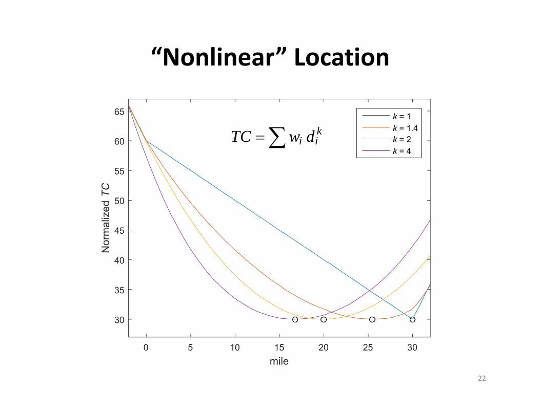
“Nonlinear” Location

0 5 10 15 20 25 30mile

30

35

40

45

50

55

60

65N

orm

aliz

ed T

Ck = 1k = 1.4k = 2k = 4

ki iTC w d

22

Minimax and Maximin Location• Minimax

– Min max distance– Set covering problem

• Maximin– Max min distance– AKA obnoxious facility location

23

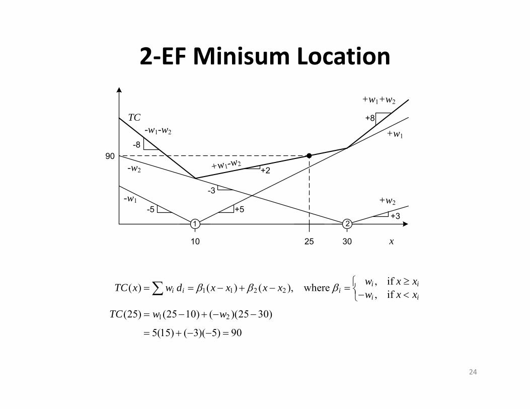
2‐EF Minisum Location

3010

-8

+8

+5

-3

+2

-5+3

1 2

25 x

TC

90

+w1

+w2

+w1+w2

-w2

-w1

-w1-w2

+w1-w2

1 1 2 2

1 2

, if ( ) ( ) ( ), where , if

(25) (25 10) ( )(25 30)

5(15) ( 3)( 5) 90

i ii i i

i i

w x xTC x w d x x x x w x x

TC w w

24

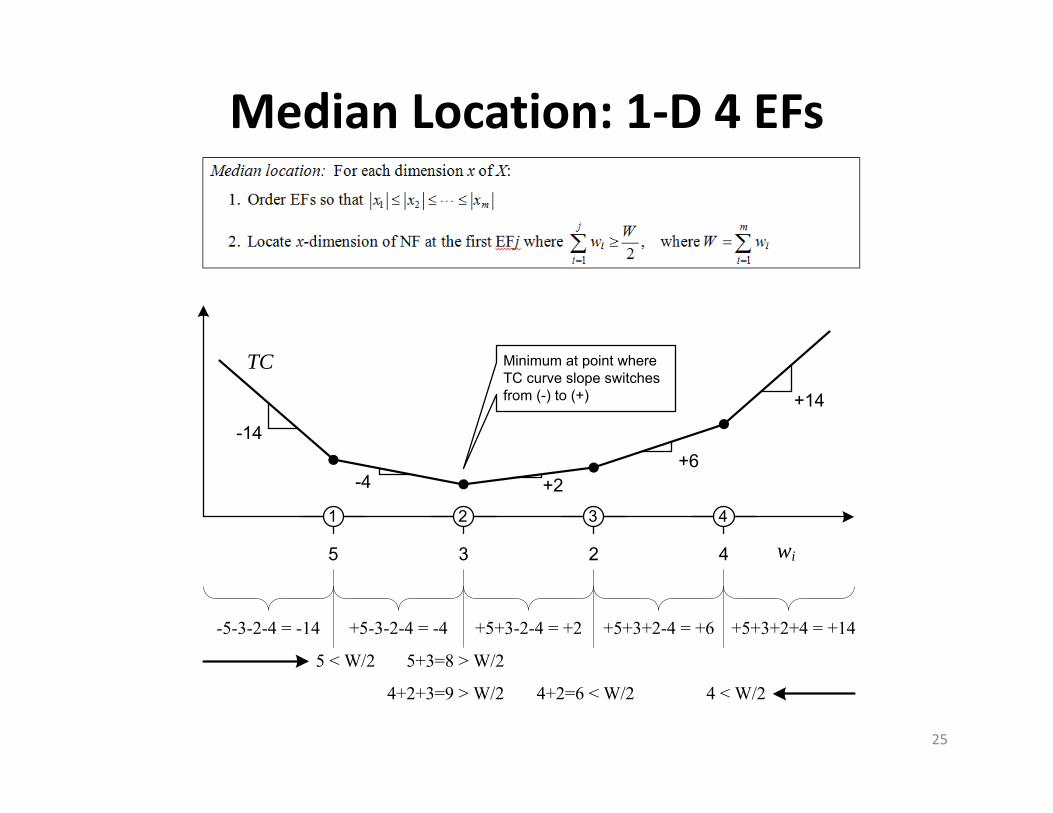
Median Location: 1‐D 4 EFs

wi

-5-3-2-4 = -14 +5-3-2-4 = -4 +5+3+2-4 = +6

Minimum at point where TC curve slope switches from (-) to (+)

5

TC

3 2 4

1 2 3 4

-14

-4 +2+6

+14

+5+3-2-4 = +2 +5+3+2+4 = +14

5 < W/2 5+3=8 > W/2

4 < W/24+2=6 < W/24+2+3=9 > W/2

25

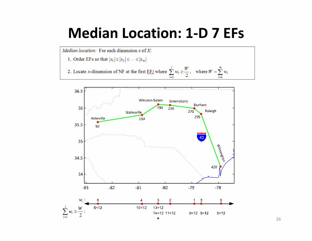
Median Location: 1‐D 7 EFs

261:

2

j

ii

Ww

:iw

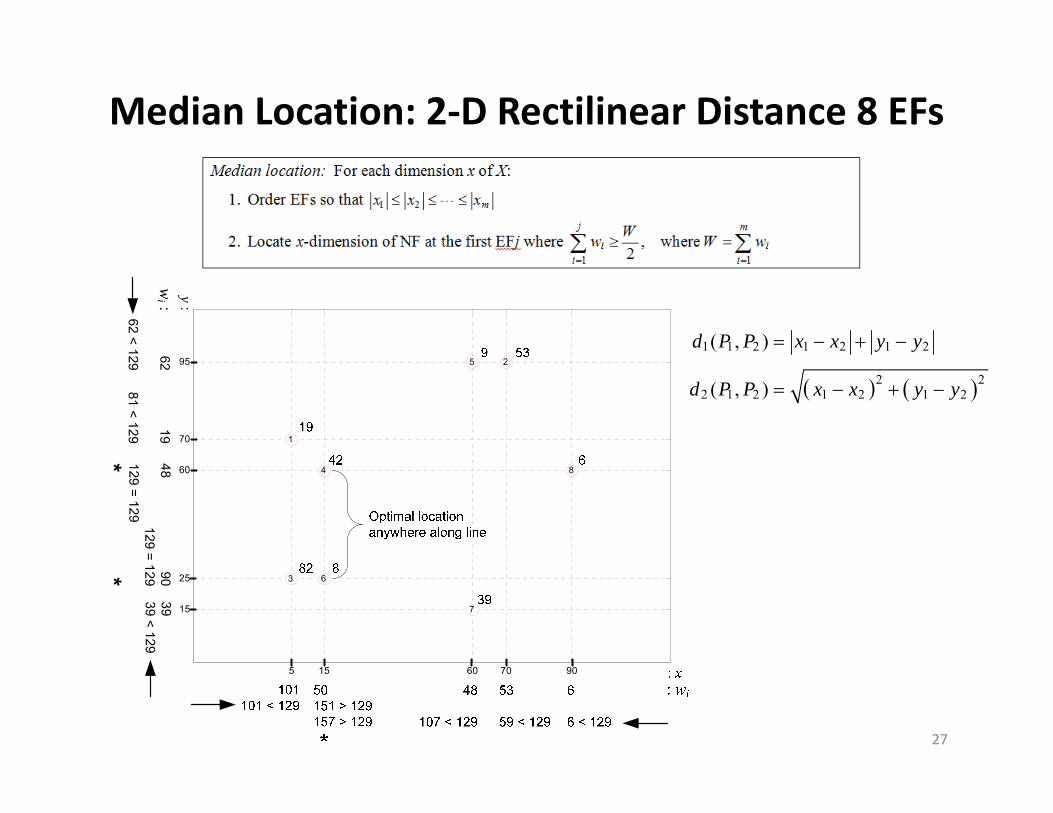
Median Location: 2‐D Rectilinear Distance 8 EFs

5 15 60 70 90

15

25

60

70

95

1

2

3

4

5

6

7

8

X

Y

62

62 < 129

19

81 < 129

48129 = 129

*

3939 < 12990

129 = 129*

wi : y:

1 1 2 1 2 1 2

2 22 1 2 1 2 1 2

( , )

( , )

d P P x x y y

d P P x x y y

27

Logistics Network for a Plant

DDDDBBBB

CustomersDCsPlantTier One

Suppliers

Tier Two Suppliers

vs.

vs.

vs.

vs.

Distribution Network

Distribution

Outbound Logistics

Finished Goods

Assembly Network

Procurement

Inbound Logistics

Raw Materials

downstream

upstream

A = B + C

B = D + E

C = F + G

28

Basic Production System

FOB (free on board)

29

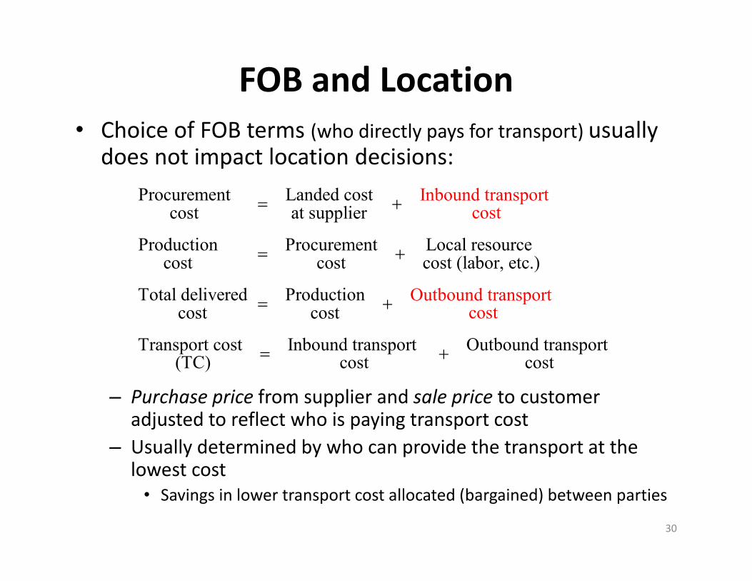
FOB and Location• Choice of FOB terms (who directly pays for transport) usually 

does not impact location decisions:

– Purchase price from supplier and sale price to customer adjusted to reflect who is paying transport cost 

– Usually determined by who can provide the transport at the lowest cost

• Savings in lower transport cost allocated (bargained) between parties

30

Procurement Landed costcost at supplier

Production Procurement Local resource cost cost cost (labor, etc.)

Total delivered Production

Inbound transport cost

Outbound transport cocost cost

Transport

s

cos

t

t (T

Inbound transport Outbound transport C) cost cost

Monetary vs. Physical Weight

31

in out

in out

(Montetary) Weight Gaining:

Physically Weight Losing:

w w

f f

1 1

min ( ) ( , ) ( , )

where total transport cost ($/yr)

monetary weight ($/mi-yr)

physical weight rate (ton/yr)

transport rate ($/ton-mi)

( , ) distance between NF at an

m m

i i i i ii i

i

i

i

i

iwTC X w d X P f r d X P

TC

w

f

r

d X P X

d EF at (mi)

NF = new facility to be located

EF = existing facility

number of EFs

i iP

m

Minisum Location: TC vs. TD• Assuming local input costs are 

– same at every location or – insignificant as compared to transport costs,

the minisum transport‐oriented single‐facility location problem is to locate NF to minimize TC

• Can minimize total distance (TD) if transport rate is same:

32

1 1

min ( ) ( , ) ( , )

where total transport distance (mi/yr)

monetary weight (trip/yr)

trips per year (trip/

transport rate =

yr)

( , ) per-trip distance between NF an E

1

d

m m

i i i i ii

i

i

i

i

i

iw

r

TD X w d X P f r d X P

TD

w

f

d X P

F (mi/trip)i

Example: Single Supplier/Customer

• The cost per ton‐mile (i.e., the cost to ship one ton, one mile) for both raw materials and finished goods is $0.10.1. Where should the plant for each product be located?2. How would location decision change if customers paid for distribution 

costs (FOB Origin) instead of the producer (FOB Destination)?• In particular, what would be the impact if there were competitors located 

along I‐40 producing the same product?

3. Which product is weight gaining and which is weight losing?4. If both products were produced in a single shared plant, why is it now 

necessary to know each product’s annual demand (fi)?33

-83 -82 -81 -80 -79 -78

34

34.5

35

35.5

36

36.5

AshevilleStatesville

Winston-Salem GreensboroDurham

Raleigh

Wilm

ington

50

150

190 220270

295

420

40

Wilmington Winston-Salem

rawmaterial

finishedgoods

ubiquitous inputs

1 ton 3 ton

2 ton

Product B

1‐D Location with Procurement and Distribution Costs

($/yr) ($/mi-yr) (mi)

monetary physicalweight weight

($/mi-yr) ($/ton-mi)(ton/yr)

i i

i i i

TC w d

w f r

in out

in out

(Montetary) Weight Gaining: 50 60

Physically Weight Losing: 150 60

w w

f f

1

:2

j

ii

Ww

:iw

Assume: all scrap is disposed of locally

34

Asheville unit offinished

good

1 tonProduction

System

Durham

NF 4

3

5

1

2

in $0.33/ton-mir out $1.00/ton-mir

3

1 1 1 1 in1

2 60 120, 40ii

f BOM f w f r

3

2 2 2 2 in1

2 60 120, 40ii

f BOM f w f r

3 3 3 out10, 10f w f r

4 4 4 out20, 20f w f r

5 5 5 out30, 30f w f r

2‐D Euclidean Distance

2 21 1,1 2 1,2

12 2

2 1 2,1 2 2,2

3 2 21 3,1 2 3,2

1 12 3 , 7 1

4 5

x p x pdd x p x pd

x p x p

x P

d

y

d 1

d 335

Minisum Distance Location

2 21 ,1 2 ,2

3

1

*

* *

1 17 14 5

( )

( ) ( )

x arg min ( )

( )

i i i

ii

d x p x p

TD d

TD

TD TD

x

P

x

x x

x

x

1 4 7x

1

2.73

5

1

d2

1 2

3

*

36

120°

Fermat’s Problem (1629):Given three points, find fourth (Steiner point) such that sum to others is minimized(Solution: Optimal location corresponds to all angles = 120°)

Minisum Weighted‐Distance Location• Solution for 2‐D+ andnon‐rectangular distances:– Majority Theorem: Locate NF at EFj if

– Mechanical (Varigon frame)– 2‐D rectangular approximation– Numerical: nonlinear unconstrained optimization

• Analytical/estimated gradient (quasi‐Newton, fminunc)

• Direct, gradient‐free (Nelder‐Mead, fminsearch)

1

*

* *

number of EFs

( ) ( )

arg min ( )

( )

m

i ii

m

TC w d

TC

TC TC

x

x x

x x

x

Varignon Frame 

 

1, where

2

m

j ii

Ww W w

37

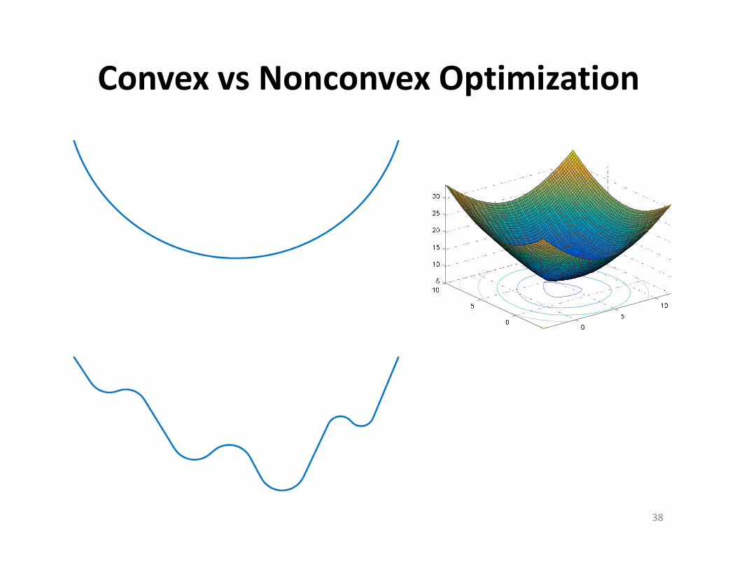
Convex vs Nonconvex Optimization

38

Gradient vs Direct Methods• Numerical nonlinear unconstrained optimization:

– Analytical/estimatedgradient

• quasi‐Newton• fminunc

– Direct, gradient‐free• Nelder‐Mead• fminsearch

39

Nelder‐Mead Simplex Method

• AKA amoeba method

• Simplex is triangle in 2‐D (dashed line in figures)

reflection expansion

outsidecontraction

insidecontraction a shrink

40

Feasible Region

41

( ), if is in , if is true( , , ) , otherwise , otherwiseTCb aiff a b c c

x x Rif a is true

return belse

return cend

Computational Geometry• Design and analysisof algorithms for solving geometric problems– Modern study started with Michael Shamos in 1975

• Facility location:– geometric data structures used to “simplify” solution procedures

-4 -3 -2 -1 0 1 2 3 4-4

-3

-2

-1

0

1

2

3

4

42

Convex Hull• Find the points that enclose all points– Most important data structure

– Calculated, via Graham’s scan in

-4 -3 -2 -1 0 1 2 3 4-4

-3

-2

-1

0

1

2

3

4

43

( log ), pointsO n n n

Delaunay Triangulation• Find the triangula‐tion of points that maximizes the minimum angle of any triangle– Captures proximity relationships

– Used in 3‐D animation

– Calculated, via divide and conquer, in

-4 -3 -2 -1 0 1 2 3 4-4

-3

-2

-1

0

1

2

3

4

44

( log ), pointsO n n n

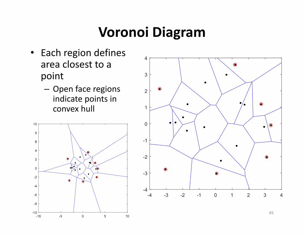
Voronoi Diagram• Each region defines area closest to a point– Open face regions indicate points in convex hull 

-4 -3 -2 -1 0 1 2 3 4-4

-3

-2

-1

0

1

2

3

4

45

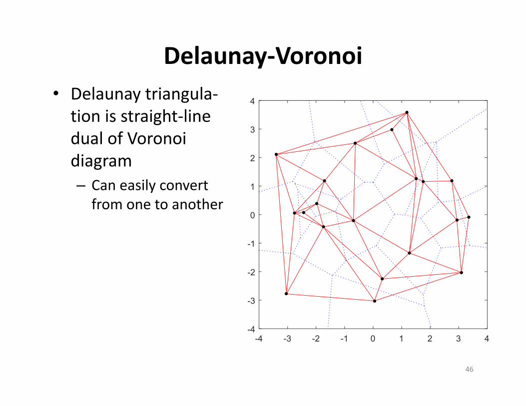
Delaunay‐Voronoi• Delaunay triangula‐tion is straight‐line dual of Voronoidiagram– Can easily convert from one to another

-4 -3 -2 -1 0 1 2 3 4-4

-3

-2

-1

0

1

2

3

4

46

Minimum Spanning Tree• Find the minimum weight set of arcs that connect all nodes in a graph– Undirected arcs:calculated, via Kruskal’s algorithm,

– Directed arcs:calculated, via Edmond’s branching algorithm, in

-4 -3 -2 -1 0 1 2 3 4-4

-3

-2

-1

0

1

2

3

4

47

( log ), arcs, nodesO m n m n

( ), arcs, nodesO mn m n

Steiner Network

48

Metric Distances

49

Chebychev Distances

50

Proof

Metric Distances using dists

3 2 2 2

3 2

4 51 'mi' 'km'dists( , , ),2 1 2 Inf3 n d m d

n m

p pD X1 X2

, 2X1 X

, 2X1 X

, 2X1 X

d

d

D

, 2X1 X

D

d = 2 d = 1

, 2X1 X Error

51

Heuristic Solutions• Most problems in logistics engineering don’t admit 

optimal solutions, only– Within some bound of optimal (provable bound, opt. gap)– Best known solution (stop when need to have solution)

• Heuristics ‐ computational effort split between– Construction: construct a feasible solution– Improvement: find a better feasible solution

• Easy construction:– any random point or permutation is feasible– can then be improved

• Hard construction:– almost no chance of generating a random feasible solution is 

possible in a single step– need to include randomness at decision points as solution is 

constructed

52

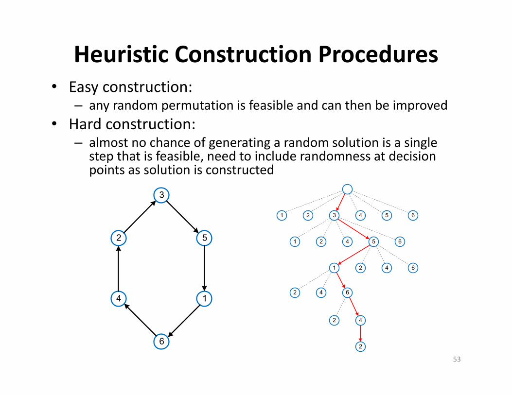
Heuristic Construction Procedures• Easy construction:

– any random permutation is feasible and can then be improved• Hard construction:

– almost no chance of generating a random solution is a single step that is feasible, need to include randomness at decision points as solution is constructed

53

1 2 3 4 5 6

1 2 4 5 6

1 2 4 6

2 4 6

2 4

2

4

2

3

5

1

6

Great Circle Distances

13.35 mi

R

54

Circuity Factor

55-80 -79.5 -79 -78.5 -78 -77.5

35

35.2

35.4

35.6

35.8

36

36.2

36.4

36.6

From High Point to Goldsboro: Road = 143 mi, Great Circle = 121 mi, Circuity = 1.19

High Point

Goldsboro

road

road 1 2 1 2

: , where usually 1.15 1.5

( , ), estimated road distance from to

i

iGC

GC

dCircuity Factor g gd

d g d P P P P

Mercator Projection

-150 -100 -50 0 50 100 150

-75

-50

-25

0

25

50

75

proj

1proj

1proj

sinh tan

tan sinh

x x

y y

y y

deg radrad deg

180and180x xx x

56

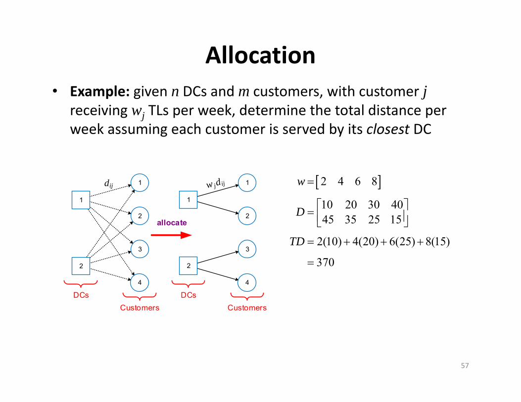
Allocation• Example: given n DCs and m customers, with customer j

receiving wj TLs per week, determine the total distance per week assuming each customer is served by its closest DC

57

2 4 6 8

10 20 30 4045 35 25 15

2(10) 4(20) 6(25) 8(15)

370

w

D

TD

2

1

3

4

CustomersDCs

ijd

1

2

2

1

3

4

CustomersDCs

j ijw d

allocate

1

2

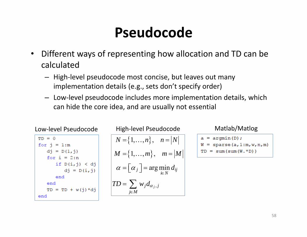
Pseudocode• Different ways of representing how allocation and TD can be 

calculated– High‐level pseudocode most concise, but leaves out many 

implementation details (e.g., sets don’t specify order)– Low‐level pseudocode includes more implementation details, which 

can hide the core idea, and are usually not essential

58

,

1, , ,

1, , ,

arg min

j

j iji N

j jj M

N n n N

M m m M

d

TD w d

Low‐level Pseudocode High‐level Pseudocode Matlab/Matlog

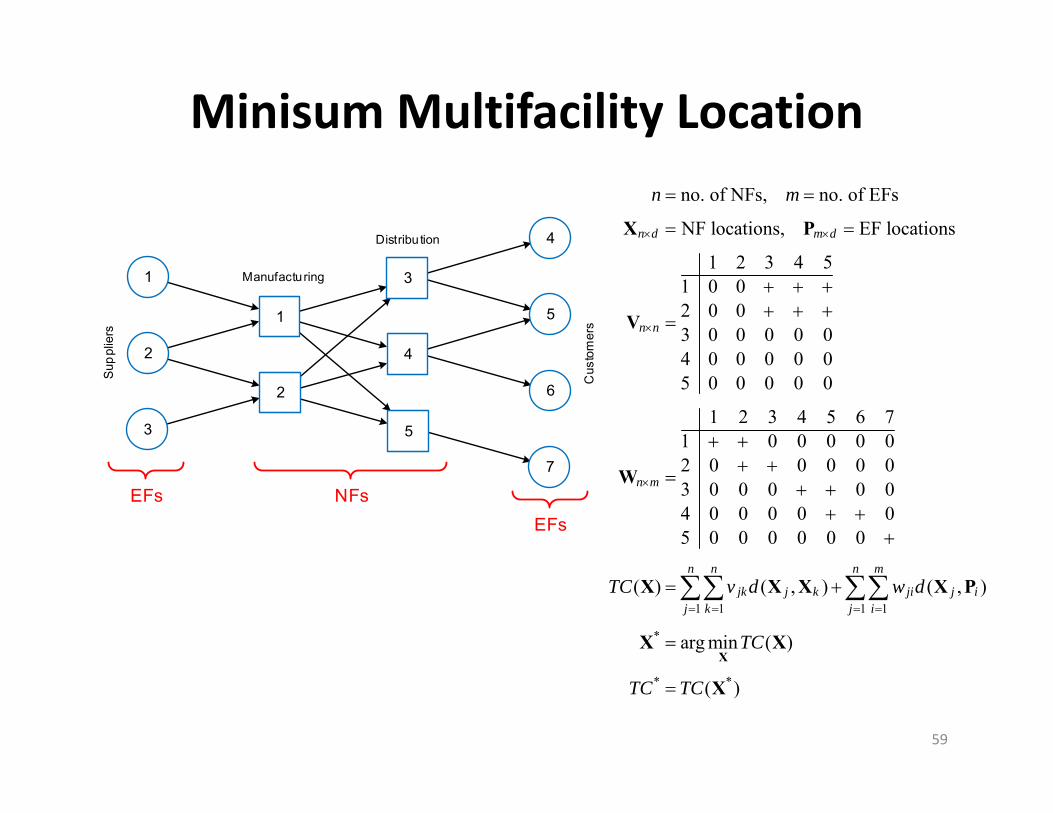
Minisum Multifacility Location

1 1 1 1

no. of NFs, no. of EFs

NF locations, EF locations

1 2 3 4 51 0 02 0 03 0 0 0 0 04 0 0 0 0 05 0 0 0 0 0

1 2 3 4 5 6 71 0 0 0 0 02 0 0 0 0 03 0 0 0 0 04 0 0 0 0 05 0 0 0 0 0 0

( ) ( , ) ( ,

n d m d

n n

n m

n n n m

jk j k ji j ij k j i

n m

TC v d w d

X P

V

W

X X X X P

*

* *

)

arg min ( )

( )

TC

TC TC

XX X

X

59

Supp

liers

Manufacturing

Cus

tom

ers

5

4

6

7

1

2

3

Distribution

NFsEFs

EFs

4

5

3

1

2

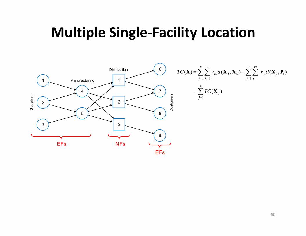
Multiple Single‐Facility Location

1 1 1 1

1

( ) ( , ) ( , )

( )

n n n m

jk j k ji j ij k j i

n

jj

TC v d w d

TC

X X X X P

X

60

Supp

liers

Manufacturing

Cus

tom

ers

7

6

8

9

4

5

1

2

3

Distribution

EFsEFs NFs

2

3

1

Facility Location–Allocation Problem• Determine both the location of n NFs 

and the allocation of flow requirements of m EFs that minimize TC

1 1

* *

, 1

* * *

(1) flow between NF and EF

total flow requirememts of EF

( , ) ( , )

, arg min ( , ) : , 0

( , )

ji ji ji ji

i

n m

ji j ij i

n

ji i jij

w r f f j i

w i

TC w d

TC w w w

TC TC

X W

X W X P

X W X W

X W

61

2

1

3

4

EFsNFs

2

3

1

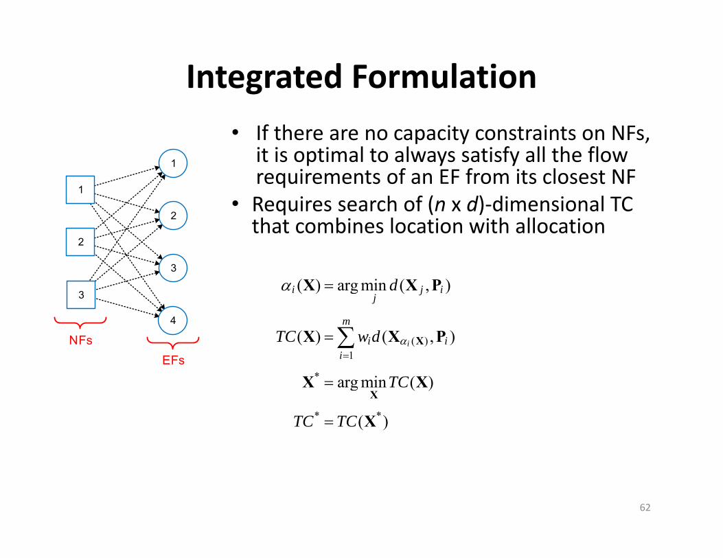
Integrated Formulation• If there are no capacity constraints on NFs, 

it is optimal to always satisfy all the flow requirements of an EF from its closest NF

• Requires search of (n x d)‐dimensional TC that combines location with allocation

( )1

*

* *

( ) arg min ( , )

( ) ( , )

arg min ( )

( )

i

i j ij

m

i ii

d

TC w d

TC

TC TC

X

X

X X P

X X P

X X

X

62

2

1

3

4

EFsNFs

2

3

1

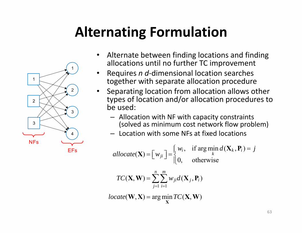
Alternating Formulation• Alternate between finding locations and finding 

allocations until no further TC improvement• Requires n d‐dimensional location searches 

together with separate allocation procedure• Separating location from allocation allows other 

types of location and/or allocation procedures to be used:– Allocation with NF with capacity constraints

(solved as minimum cost network flow problem)– Location with some NFs at fixed locations

1 1

, if arg min ( , )( )

0, otherwise

( , ) ( , )

( , ) arg min ( , )

i k ikji

n m

ji j ij i

w d jallocate w

TC w d

locate TC

X

X PX

X W X P

W X X W

63

2

1

3

4

EFsNFs

2

3

1

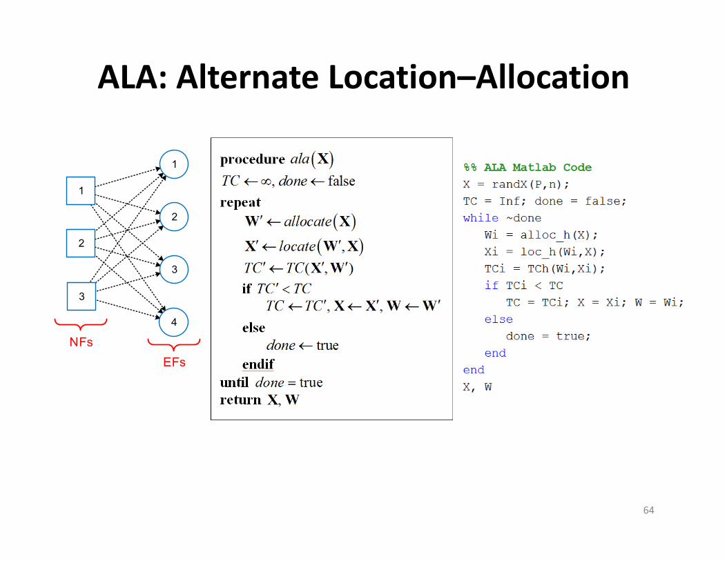
ALA: Alternate Location–Allocation

64

2

1

3

4

EFsNFs

2

3

1

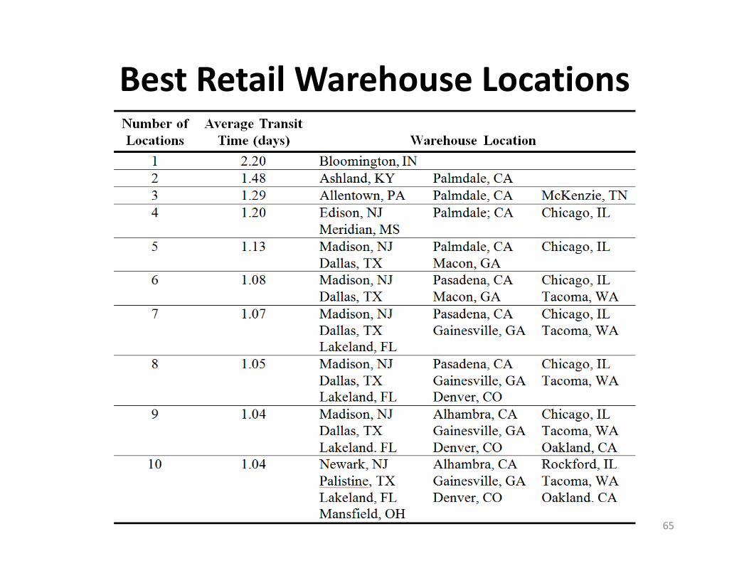
Best Retail Warehouse Locations

65

Aggregate Demand Point Data Sources• Aggregate demand point: centroid of population• Good rule of thumb: use 100x number of NFs ( 1000 pts provides 

good coverage for locating  10 NFs)1. City data: ONLY USE FOR LABELING!, not as demand points2. 3‐digit ZIP codes:  1000 pts covering U.S., = 20 pts NC3. County data:  3000 pts covering U.S., = 100 pts NC

– Grouped by state or CSA (Combined Statistical Area)– CSA = defined by set of counties (174 CSAs in U.S.)– FIPS code = 5‐digit state‐county FIPS code

= 2‐digit state code + 3‐digit county code= 37183 = 37 NC FIPS + 183 Wake FIPS

– CSA List: www2.census.gov/programs‐surveys/metro‐micro/geographies/reference‐files/2017/delineation‐files/list1.xls

4. 5‐digit ZIP codes: > 35KptsU.S., 1000 ptsNC5. Census Block Group: > 220K pts U.S.,  1000 pts Raleigh‐Durham‐

Chapel Hill, NC CSA– Grouped by state, county, or CSA

66

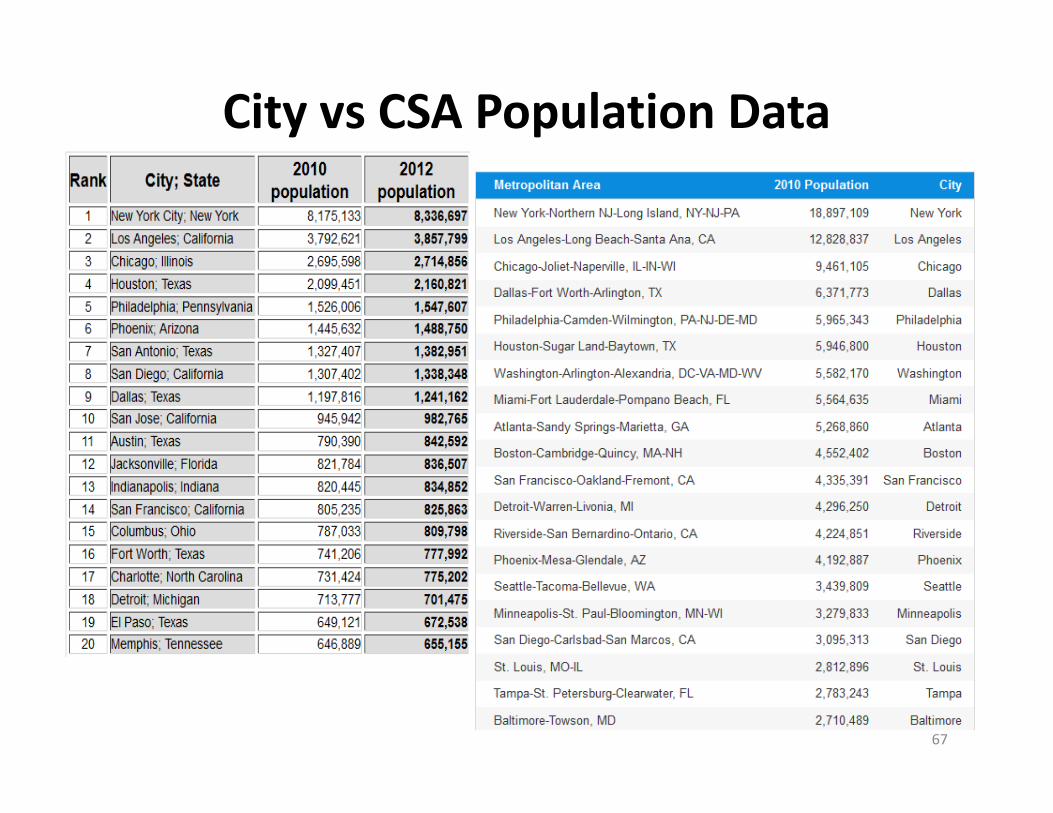
City vs CSA Population Data

67

Demand Point Aggregation• Existing facility (EF): actual physical location of demand source• Aggregate demand point: single location representing 

multiple demand sources

68

-83 -82 -81 -80 -79 -78

34

34.5

35

35.5

36

36.5

AshevilleStatesville

Winston-Salem GreensboroDurham

Raleigh

Wilm

ington

50

150

190 220270

295

420

40

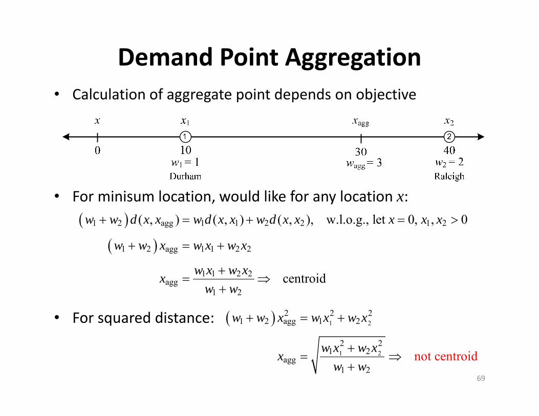
Demand Point Aggregation• Calculation of aggregate point depends on objective

• For minisum location, would like for any location x: 

• For squared distance:

69

1 2 agg 1 1 2 2 1 2

1 2 agg 1 1 2 2

1 1 2 2agg

1 2

( , ) ( , ) ( , ), w.l.o.g., let 0, , 0

centroid

w w d x x w d x x w d x x x x x

w w x w x w x

w x w xxw w

1 2

1 2

2 2 21 2 agg 1 2

2 21 2

agg1 2

not centroid

w w x w x w x

w x w xxw w

Optimal Number of NFs

70

Uncapacitated Facility Location (UFL)• NFs can only be located at discrete set of sites

– Allows inclusion of fixed cost of locating NF at site– Variable costs are usually transport cost from NF to EF– Total of 2n – 1 potential solutions (all nonempty subsets of sites)

71

1,..., , existing facilites (EFs)

1,..., , sites available to locate NFs, set of EFs served by NF at site

variable cost to serve EF from NF at site fixed cost locating NF at site

, s

i

ij

i

M m

N nM M ic j ik iY N

*

*

ites at which NFs are located

arg min :

min cost set of sites where NFs located

number of NFs located

i

i ij iY i Y i Y j M i Y

Y k c M M

Y

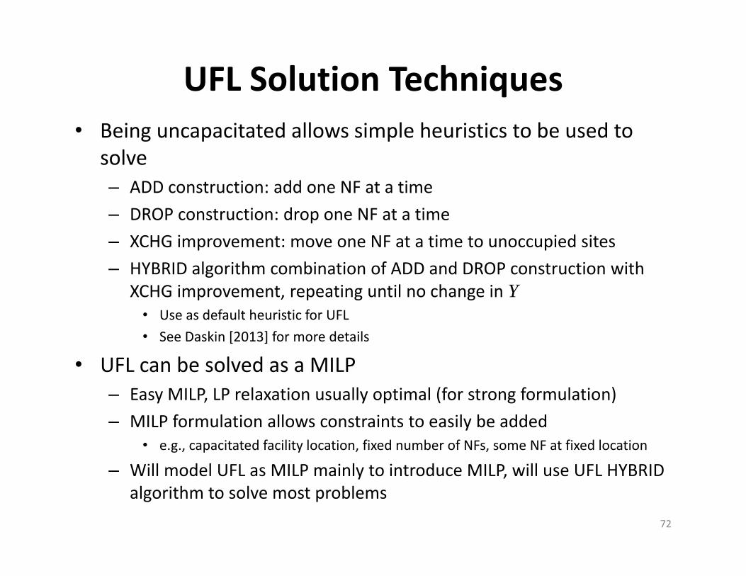
UFL Solution Techniques• Being uncapacitated allows simple heuristics to be used to 

solve– ADD construction: add one NF at a time– DROP construction: drop one NF at a time– XCHG improvement: move one NF at a time to unoccupied sites– HYBRID algorithm combination of ADD and DROP construction with 

XCHG improvement, repeating until no change in Y• Use as default heuristic for UFL• See Daskin [2013] for more details

• UFL can be solved as a MILP– Easy MILP, LP relaxation usually optimal (for strong formulation)– MILP formulation allows constraints to easily be added

• e.g., capacitated facility location, fixed number of NFs, some NF at fixed location

– Will model UFL as MILP mainly to introduce MILP, will use UFL HYBRID algorithm to solve most problems

72

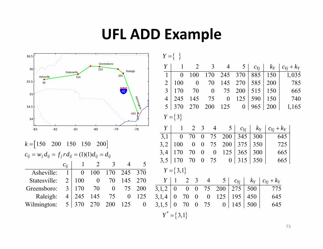
UFL ADD Example

73

150 200 150 150 200(1)(1)1 2 3 4 5

Asheville: 1 0 100 170 245 370Statesville: 2 100 0 70 145 270

Greensboro: 3 170 70 0 75 200Raleigh: 4 245 145 75 0 125

Wilmington: 5 370 270 200 125 0

ij j ij j ij ij ij

ij

kc w d f rd d d

c

‐83 ‐82 ‐81 ‐80 ‐79 ‐78

34

34.5

35

35.5

36

36.5

 Asheville Statesville 

 Greensboro

 Raleigh

50 

150 

220

 295

 420

40

1 2 3 4 51 0 100 170 245 370 885 150 1,0352 100 0 70 145 270 585 200 7853 170 70 0 75 200 515 150 6654 245 145 75 0 125 590 150 7405 370 270 200 125 0 965 200 1,165

Yj Y Yj YY c k c k

1 2 3 4 53,1 0 70 0 75 200 345 300 6453, 2 100 0 0 75 200 375 350 7253, 4 170 70 0 0 125 365 300 6653,5 170 70 0 75 0 315 350 665

Yj Y Yj YY c k c k

1 2 3 4 53,1,2 0 0 0 75 200 275 500 7753,1,4 0 70 0 0 125 195 450 6453,1,5 0 70 0 75 0 145 500 645

Yj Y Yj YY c k c k

Y

3Y

3,1Y

* 3,1Y

UFLADD: Add Construction Procedure

74

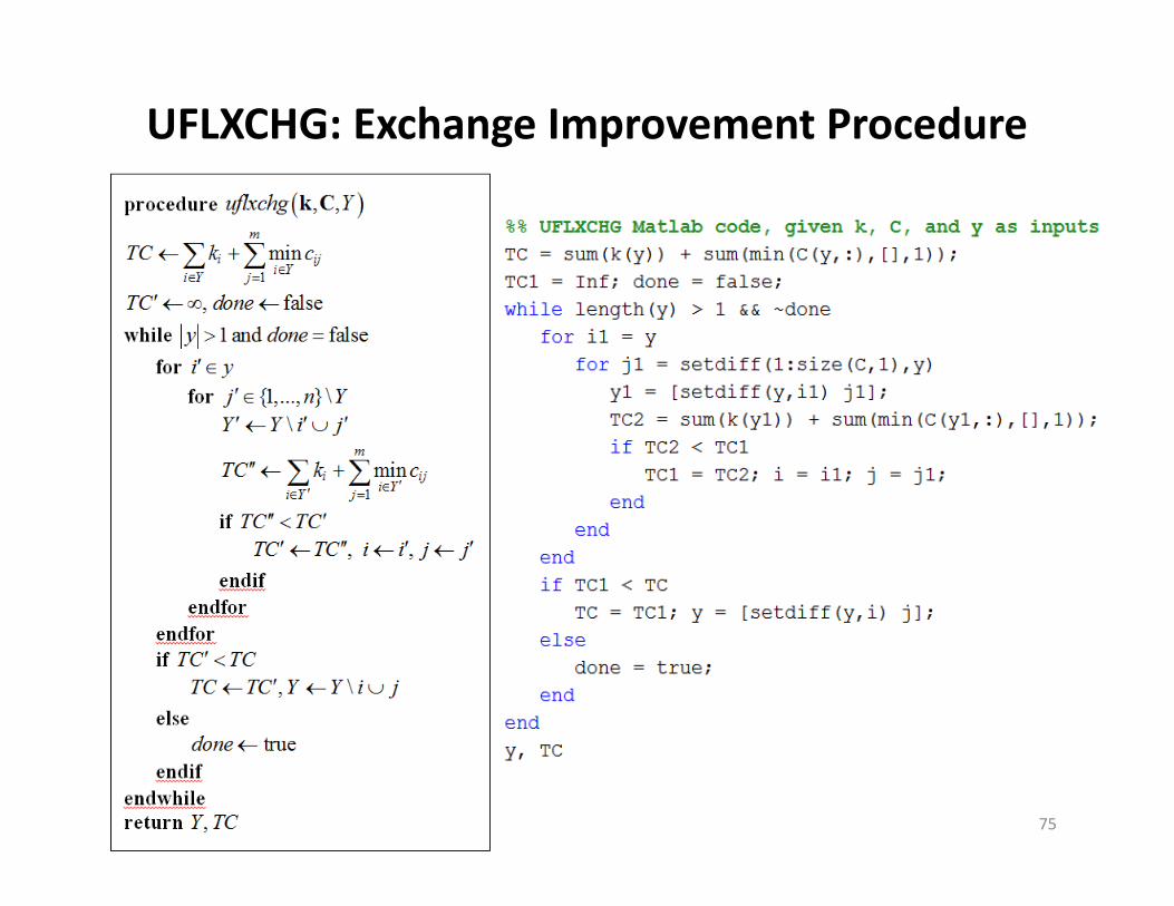
UFLXCHG: Exchange Improvement Procedure

75

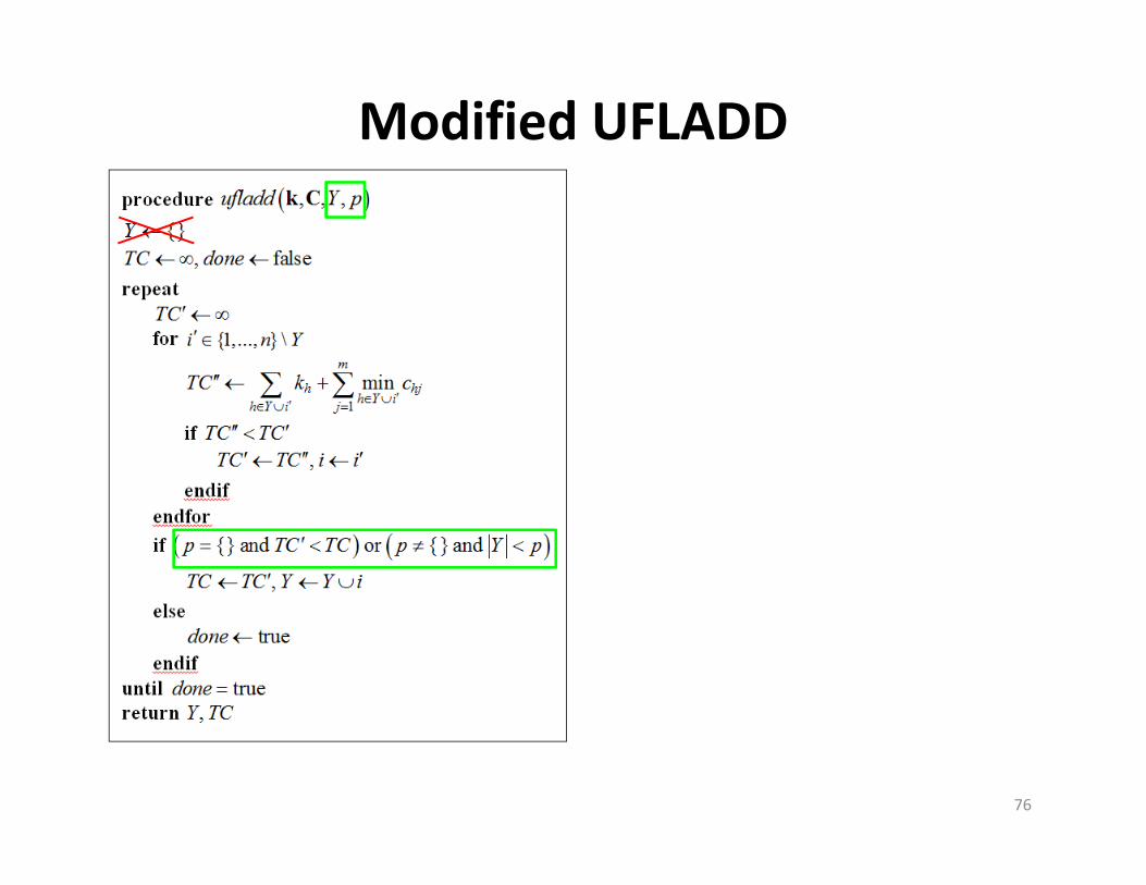
Modified UFLADD

76

UFL: Hybrid Algorithm

77

P‐Median Location Problem• Similar to UFL, except

– Number of NF has to equal p (discrete version of ALA)– No fixed costs

78

*

number of NFs

arg min : ,i

ij iY i Y j M i Y

p

Y c M M Y p

Bottom‐Up vs Top‐Down Analysis• Bottom‐Up: HW 3 Q 3

3 2

1 2 2 3 3 1

1 2 2 3 3 1

3

1

*

* *

cary

cary

lon-lat of EFs

48,24,35 (TL/yr)

2 ($/TL-mi)

1 ( , ) ( , ) ( , )3 ( , ) ( , ) ( , )

( ) ( , )

argmin ( )

( )

lon-lat of Cary

(

RD RD RD

GC GC GC

i GC ii

r

d d dgd d d

TC f rgd

TC

TC TC

TC TC

x

P

f

P P P P P PP P P P P P

x x P

x x

x

xcary

cary *

)

TC TC TC

x

• Top‐Down: estimate r(circuity factor cancels, so not needed, HW 4 Q 4)

cary

cary

nom 3cary

1

3

nom1

*

* *

cary *

current known , 10 ton /TL

480,240,350 (ton /yr)

($/ton-mi)( , )

( ) ( , )

argmin ( )

( )

i GC ii

i GC ii

TC TC

TCrf d

TC f r d

TC

TC TC

TC TC TC

x

f

x P

x x P

x x

x

79

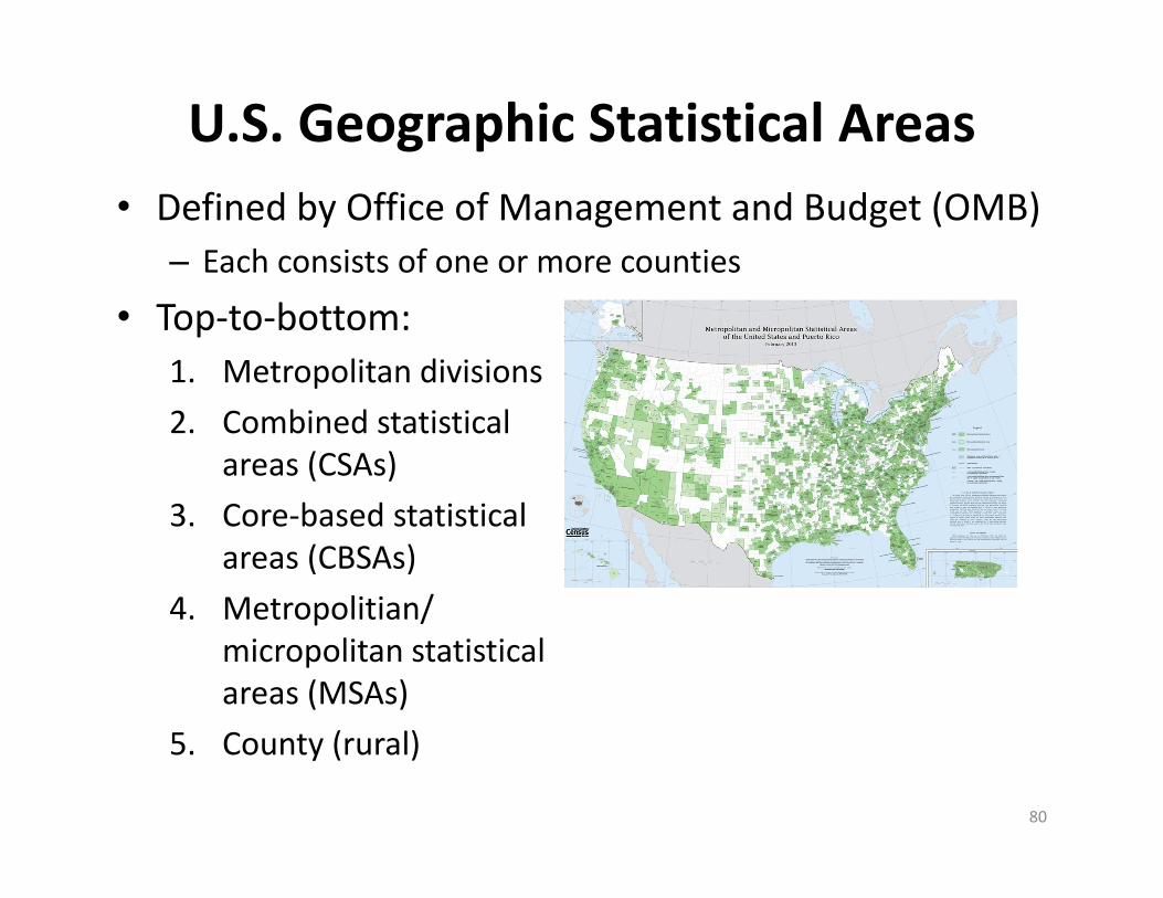
U.S. Geographic Statistical Areas• Defined by Office of Management and Budget (OMB)

– Each consists of one or more counties

• Top‐to‐bottom:1. Metropolitan divisions2. Combined statistical

areas (CSAs)3. Core‐based statistical

areas (CBSAs)4. Metropolitian/

micropolitan statisticalareas (MSAs)

5. County (rural)

80

Transport Cost if NF at every EF

1 52 3 4 6

Facility Fixed + Transport Cost

Facility Fixed Cost

Transport Cost

TC

Number of NFsNF = EF

0 ?

81

transport costfixed cost

i

i iji Y i Y j M

TC k c

Area Adjustment for Aggregate Data Distances• LB: avg. dist. from center to all points in area• UB: avg. dist. between all random pairs of points• Local circuity factor = 1.5, regular non‐local = 1.2

20

0

0

0 0 0

2

0.402

32 0.51515

2

0.45

LB

LB

UB

LB UB

a d

ad a

ad a

d d d a

Mathai, A.M., An Intro to Geo Prob, p. 207 (2.3.68)

82

2a

a0LB

d

0UB

d

a

1 2 1 2 local 1 2

1 2 1 2

( , ) max ( , ), 0.45max ,

max 1.2 ( , ), 0.675max ,

a GC

GC

d gd g a a

d a a

X X X X

X X

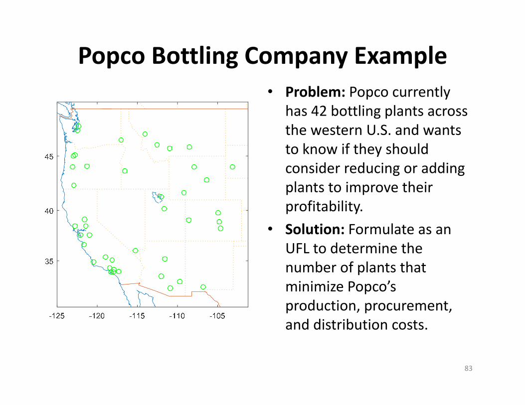
Popco Bottling Company Example• Problem: Popco currently 

has 42 bottling plants across the western U.S. and wants to know if they should consider reducing or adding plants to improve their profitability.

• Solution: Formulate as an UFL to determine the number of plants that minimize Popco’sproduction, procurement, and distribution costs.

83

Popco Bottling Company Example• Following representative information is available for each of N

current plants (DC) i:

• Assuming plants are (monetarily) weight gaining since they are bottling plants, so UFL can ignore inbound procurement costs related to location

84

location

aggregate production (tons)

total production and procurement cost

total distribution cost

i

DCi

i

i

xy

f

TPC

TDC

Popco Bottling Company Example

1. Use plant (DC) production costs to find UFL fixed costs via linear regression

– variable production costs cp do not change and can be cut

only keep for UFL

i

DCi p

i N i NTPC TPC c fk

k

85

• Difficult to estimate fixed cost of each new facility because this cost must not include any cost related to quantity of product produced at facility.

Popco Bottling Company Example2. Allocate all 3‐digit ZIP 

codes to closest plant (up to 200 mi max) to serve as aggregate customer demand points.

-125 -120 -115 -110 -105

35

40

45

max

max

: arg min and

200 mi

a ai hj ij

h

ii N

M j d i d d

d

M M

86

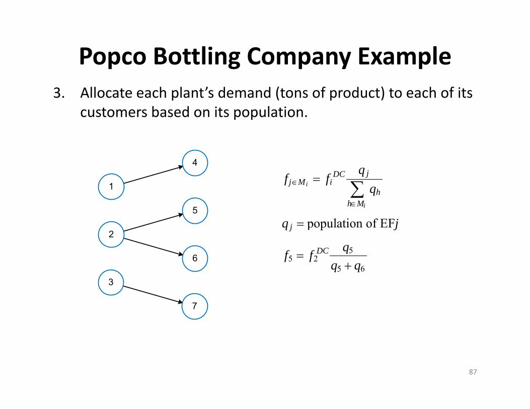
Popco Bottling Company Example3. Allocate each plant’s demand (tons of product) to each of its 

customers based on its population.

55 2

5 6

population of EF

i

i

jDCj M i

hh M

j

DC

qf f

q

q j

qf fq q

5

4

6

7

1

2

3

87

Popco Bottling Company Example4. Estimate a nominal transport rate ($/ton‐mi) using the ratio 

of total distribution cost ($) to the sum of the product of the demand (ton) at each customer and its distance to its plant (mi).

nom

j

ii N

aj ij

i N j M

TDCr

f d

88

Popco Bottling Company Example5. Calculate UFL variable transportation cost cij ($) for each 

possible NF site i (all customer and plant locations) and EF site j (all customer locations) as the product of customer jdemand (ton), distance from site i to j (mi), and the nominal transport rate ($/ton‐mi).

6. Solve as UFL, where TC returned includes all new distribution costs and the fixed portion of production costs.

noma

i M Nij j ij i M Nj M j M

c r f d

C

89

transport costfixed cost

, number of potential NF sites

, number of EF sites

i

i iji Y i Y j M

TC k c

n M N

m M

MILP

LP: max 's.t.

0MILP: some integer

ILP: integerBLP: 0,1

ix

c xAx b

x

xx

90

1 42 63 5

1

2

3

0

4

1x

2x

1 2

1 2

1

1 2

max 6 8s.t. 2 3 11

2 7, 0

x xx xx

x x

6 8

2 3 11,2 0 7

c

A b

* *

13 22 , 311 313

x c x

Branch and Bound

1 42 63 5

1

2

3

0

4

2313

1 2

1 2

1

1 2

1 2

max 6 8s.t. 2 3 11

2 7, 0, integer

x xx xx

x xx x

1x

6 8

2 3 11,2 0 7

c

A b

2x

01

2

1313

26

31

2303

28

30

345

6

0

1 8

32

74

65

231 , 03

UB LB

1 3x 1 4x

2 1x 2 2x

1 2x 1 3x

2 2x 2 3x

LP

131 , 03

UB LB

131 , 263

UB LB

Incumbent 31, 26UB LB

230 , 263

UB LB

Incumbent

230 , 303230 30 13

UB LB

gap

230 , 283

UB LB

Incumbent

Fathomed,infeasible

Fathomed,infeasible

STOP

91

MILP Solvers

92

MILP Solvers

2313

1x

2x

1 2 1 2

1 2

2 2 1, , 0 and integer

0

x x x x

x x

• Presolve: eliminate variables

• Cutting planes: keeps all integer solutions and cuts off LP solutions (Gomory cut)

• Heuristics: find good initial incumbent solution

• Parallel: use separate cores to solve nodes in B&B tree

• Speedup from 1990‐2014:– 320,000 computer speed– 580,000 algorithm improvements

93

Gomory cut

MILP Formulation of UFL

min

s.t. 1,

,

0 1, ,

0,1 ,

i i ij iji N i N j M

iji N

i ijj M

ij

i

k y c x

x j M

my x i N

x i N j M

y i N

, ,i ijy x i N j M

wherefixed cost of NF at site 1,...,

variable cost from to serve EF 1,...,

1, if NF established at site 0, otherwise

fraction of EF demand served from NF at site .

i

ij

i

ij

k i N n

c i j M m

iy

x j i

94

(Weighted) Set Covering

*

1,..., , objects to be covered

, 1,..., , subsets of cost of using in cover

arg min : , min cost covering of

i

i i

i iI i I i I

M m

M M i N n Mc M

I c M M M

95

*

1 2 3

4 5

*

1,...,6

1,...,5

1, 2 , 1, 4,5 , 3,5

2,3,6 , 61, for all

arg min :

2, 4

2

i

i iI i I i I

ii I

M

i N

M M M

M Mc i N

I c M M

c

1

4

2

5

3

6

M2

M1

M3

M4

M5

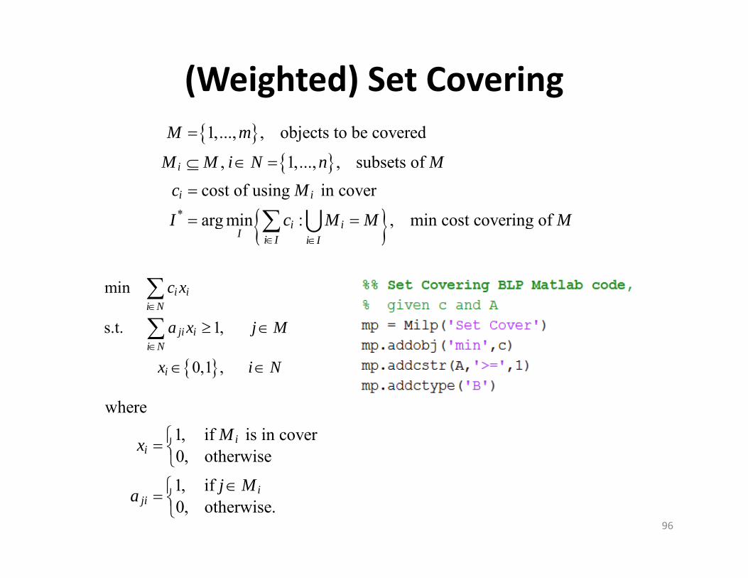
(Weighted) Set Covering

min

s.t. 1,

0,1 ,

i ii N

ji ii N

i

c x

a x j M

x i N

*

1,..., , objects to be covered

, 1,..., , subsets of cost of using in cover

arg min : , min cost covering of

i

i i

i iI i I i I

M m

M M i N n Mc M

I c M M M

where1, if is in cover0, otherwise

1, if 0, otherwise.

ii

iji

Mx

j Ma

96

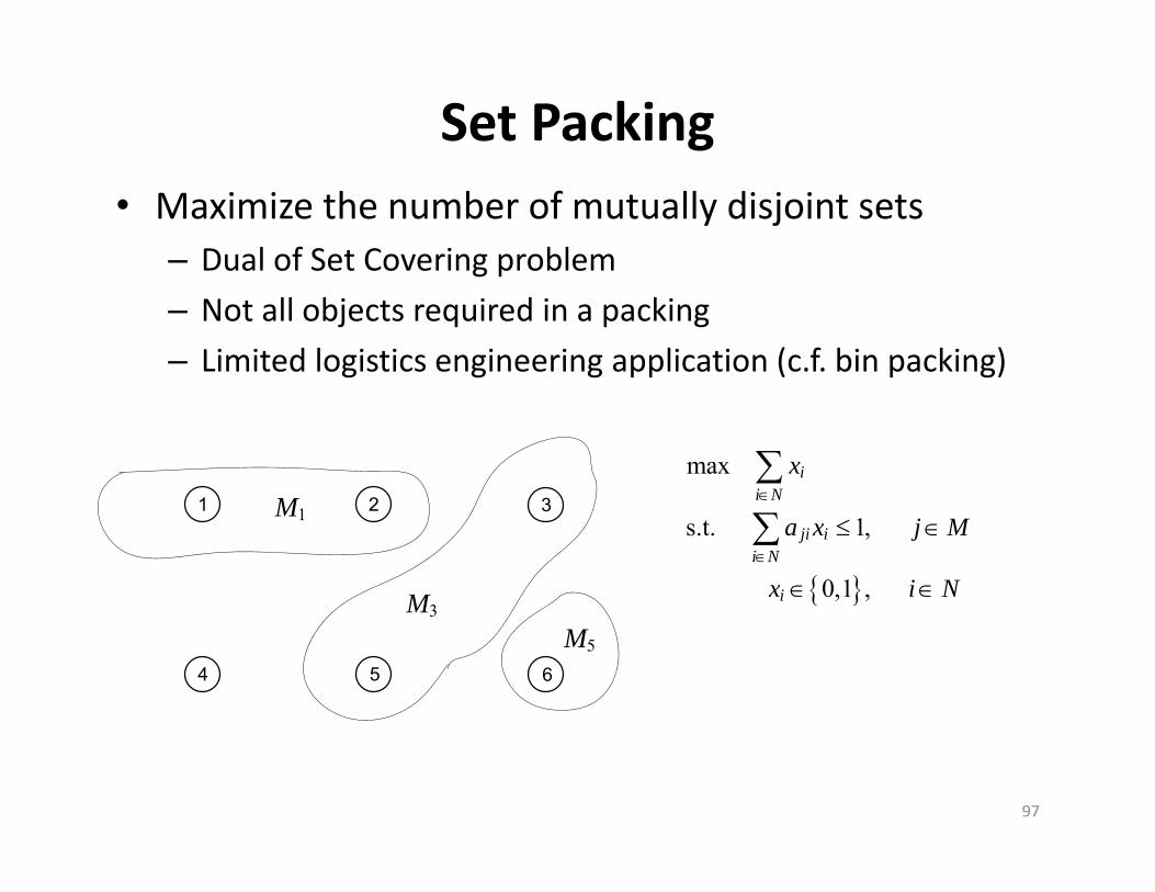
Set Packing• Maximize the number of mutually disjoint sets

– Dual of Set Covering problem– Not all objects required in a packing– Limited logistics engineering application (c.f. bin packing)

97

max

s.t. 1,

0,1 ,

ii N

ji ii N

i

x

a x j M

x i N

1

4

2

5

3

6

M1

M3

M5

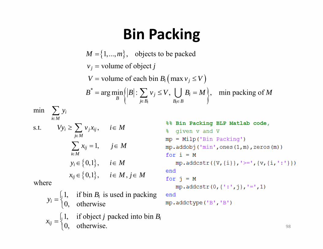
Bin Packing

min

s.t. ,

1,

0,1 ,

0,1 , ,

ii M

i j ijj M

iji M

i

ij

y

Vy v x i M

x j M

y i M

x i M j M

*

1,..., , objects to be packedvolume of object

volume of each bin max

arg min : , , min packing of i i

j

i j

j iB j B B B

M mv j

V B v V

B B v V B M M

where1, if bin is used in packing0, otherwise

1, if object packed into bin 0, otherwise.

ii

iij

By

j Bx

98

Topics1. Introduction2. Facility location3. Freight transport

– Exam 1 (take home)

4. Network models5. Routing

– Exam 2 (take home)

6. Warehousing– Final project– Final exam (in class)

99

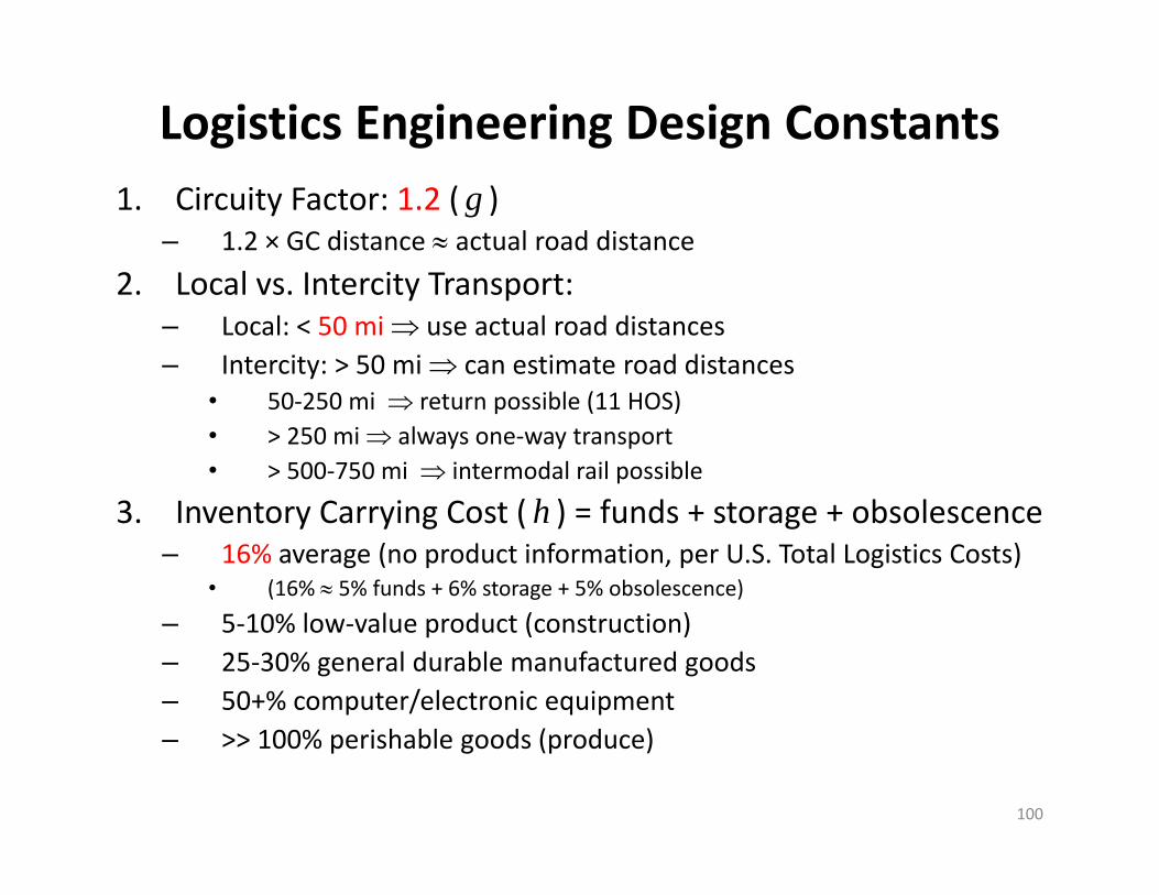
Logistics Engineering Design Constants1. Circuity Factor: 1.2 ( g )

– 1.2 × GC distance  actual road distance2. Local vs. Intercity Transport:

– Local: < 50 mi use actual road distances– Intercity: > 50 mi  can estimate road distances

• 50‐250 mi  return possible (11 HOS)• > 250 mi  always one‐way transport• > 500‐750 mi  intermodal rail possible

3. Inventory Carrying Cost ( h ) = funds + storage + obsolescence– 16% average (no product information, per U.S. Total Logistics Costs)

• (16%  5% funds + 6% storage + 5% obsolescence)

– 5‐10% low‐value product (construction)– 25‐30% general durable manufactured goods– 50+% computer/electronic equipment– >> 100% perishable goods (produce)

100

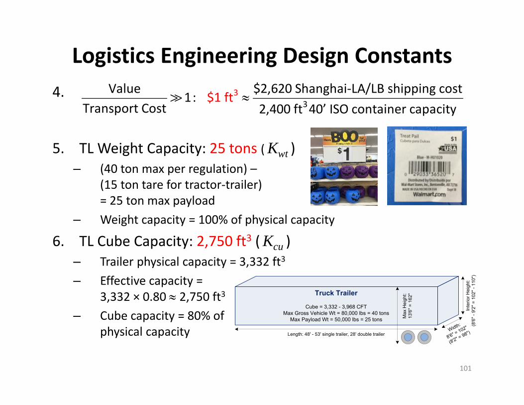
Logistics Engineering Design Constants4.

5. TL Weight Capacity: 25 tons ( Kwt )– (40 ton max per regulation) –

(15 ton tare for tractor‐trailer)= 25 ton max payload

– Weight capacity = 100% of physical capacity

6. TL Cube Capacity: 2,750 ft3 (Kcu )– Trailer physical capacity = 3,332 ft3

– Effective capacity = 3,332 × 0.80  2,750 ft3

– Cube capacity = 80% of physical capacity

33 $2,620 Shanghai‐LA/LB shipping cost

2,400Value

1:Transport Cost ft  40’ ISO container capa

$1 ftcity

101

Truck Trailer

Cube = 3,332 - 3,968 CFTMax Gross Vehicle Wt = 80,000 lbs = 40 tons

Max Payload Wt = 50,000 lbs = 25 tons

Length: 48' - 53' single trailer, 28' double trailer

Inte

rior H

eigh

t:(8

'6" -

9'2"

= 1

02" -

110"

)

Width:

8'6" = 102"

(8'2" = 98")

Max

Hei

ght:

13

'6" =

162

"

Logistics Engineering Design Constants7. TL Revenue per Loaded Truck‐Mile: $2/mi in 2004 ( r )

– TL revenue for the carrier is your TL cost as a shipper

15%, average deadhead travel

$1.60, cost per mile in 2004

$1.60$1.88, cost per loaded‐mile

1 0.156.35%, average operating margin for trucking

$1.88$2.00, revenue per loaded‐mile

1 0.0635102

Truck Shipment Example• Product is to be shipped in cartons 

from Raleigh, NC (27606) to Gainesville, FL (32606). Each unit weighs 40 lb and occupies 9 ft3, and units can be stacked on top of each other in a trailer.

• One‐Time Shipments (operational decision): know q– Know when and how much to ship, 

need to determine if TL and/or LTL to be used

• Periodic Shipments (tactical decision): know f, determine q– Need to determine how often and 

how much to ship

103

Truck Shipment Example: One‐Time1. Assuming that the product is to be shipped P2P TL, what is 

the maximum payload for each trailer used for the shipment?

max

3

33

maxmax

max max max

25 ton

2750 ft

40 lb/unit 4.4444 lb/ft9 ft /unit

20002000

min , min ,2000

4.4444(2750)min 25, 6.1111 ton2000

wtwt

cu

cucucu

cu

cuwt cuwt

q K

K

s

q sKK qs

sKq q q K

104

Truck Shipment Example: One‐Time2. Next Monday, 350 units of the product are to be shipped. 

How many truckloads are required for this shipment?

3. Using the most recent rate estimate available, what is the TL transport charge for this shipment?

max

40 7350 7 ton, 2 truckloads2000 6.1111

qqq

July 2017

20042004

max

532 mi

$2.00 / mi102.7

124.3 $2.00 / mi $2.420643 / mi102.7

7 (2.420643)(532) $2,575.566.1111

TLTL

TL

TL

d

PPI PPIr rPPI

qc r dq

105

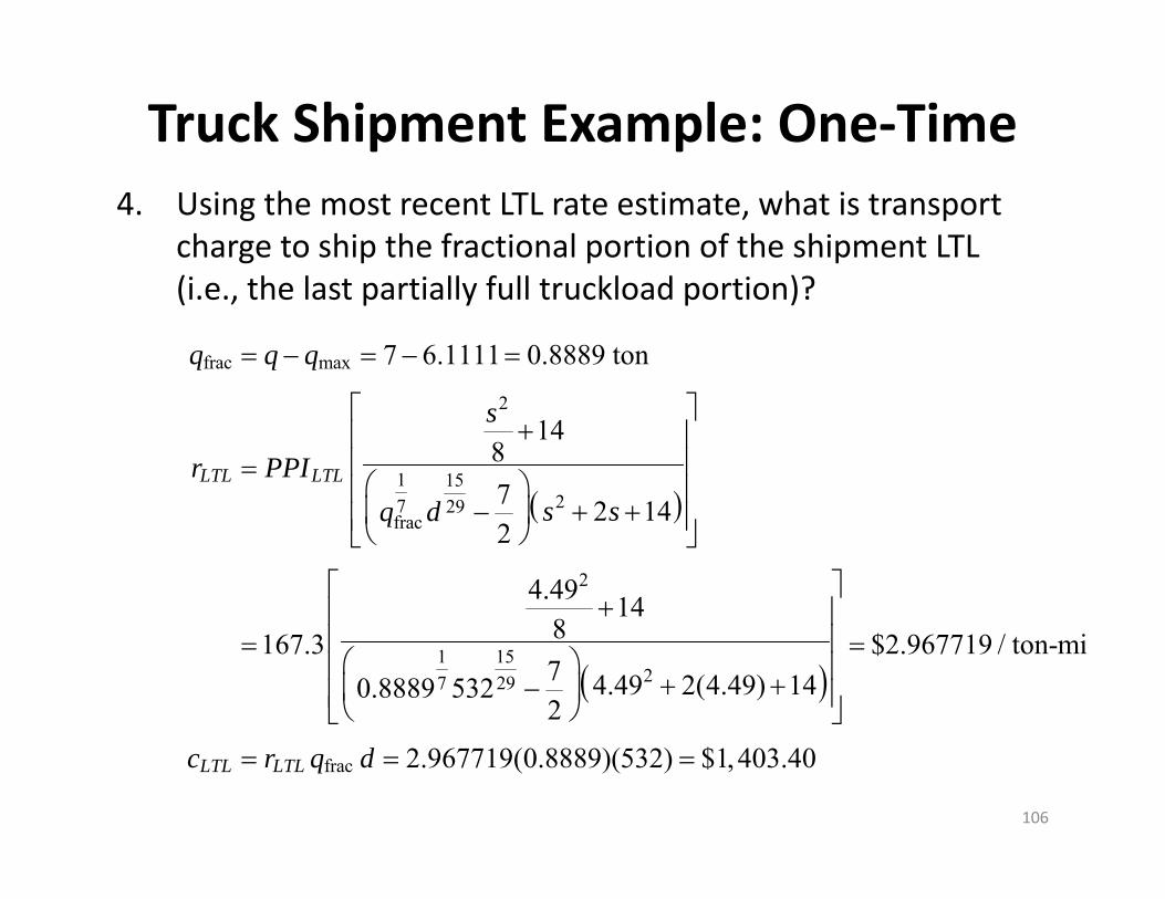
Truck Shipment Example: One‐Time4. Using the most recent LTL rate estimate, what is transport 

charge to ship the fractional portion of the shipment LTL (i.e., the last partially full truckload portion)?

frac max

2

1 1527 29

frac

2

1 1527 29

frac

7 6.1111 0.8889 ton

1487 2 142

4.49 148167.3 $2.967719 / ton-mi7 4.49 2(4.49) 140.8889 5322

2.967719(0.

LTL LTL

LTL LTL

q q q

s

r PPIs sq d

c r q d

8889)(532) $1,403.40

106

Truck Shipment Example: One‐Time5. What is the change in total charge associated with the 

combining TL and LTL as compared to just using TL?

1

fracmax max

$115.62

TL TL LTL

LTL

c c c c

q qr d r d r q dq q

107

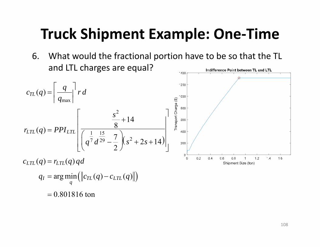
Truck Shipment Example: One‐Time6. What would the fractional portion have to be so that the TL 

and LTL charges are equal?

max

2

1 1527 29

( )

148( )7 2 142

( ) ( )

arg min ( ) ( )

0.801816 ton

TL

LTL LTL

LTL LTL

I TL LTLq

qc q r dq

s

r q PPIs sq d

c q r q qd

q c q c q

108

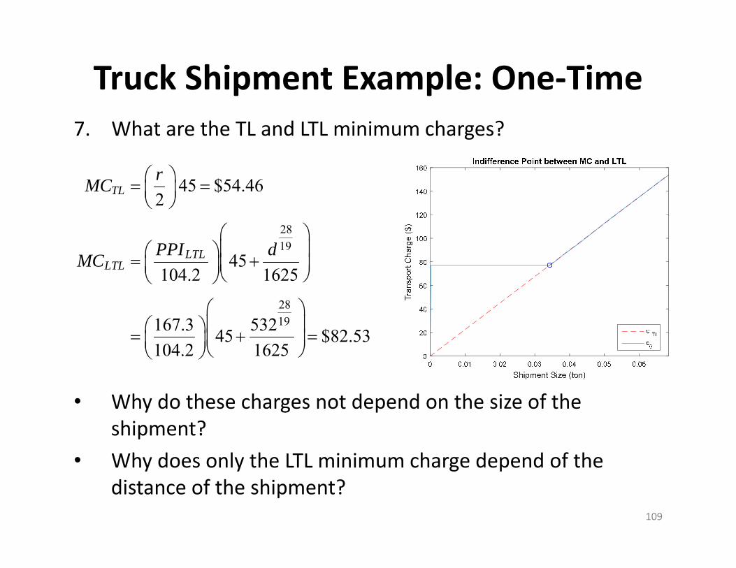
Truck Shipment Example: One‐Time7. What are the TL and LTL minimum charges?

• Why do these charges not depend on the size of the shipment?

• Why does only the LTL minimum charge depend of the distance of the shipment?

2819

2819

45 $54.462

45104.2 1625

167.3 53245 $82.53104.2 1625

TL

LTLLTL

rMC

PPI dMC

109

Truck Shipment Example: One‐Time• Independent Transport Charge ($):

0 ( ) min max ( ), , max ( ),TL TL LTL LTLc q c q MC c q MC

0 1 2 3 4 5 6 7Shipment Size (ton)

0

500

1000

1500

2000

2500

3000

Tran

spor

t Cha

rge

($)

Independent shipment charge: Class 200 from 27606 to 32606

110

Truck Shipment Example: One‐Time8. Using the same LTL shipment, find online one‐time (spot) LTL 

rate quotes using the FedEx LTL website

3

3

40 lb/unit9 ft /unit

4.4444 lb/ft

Class 200

s

Class‐Density Relationshipfrac 0.8889 ton

0.8889(2000) 1778 lb

q

• Most likely freight class:

• What is the rate quote for the reverse trip from Gainesville (32606) to Raleigh (27606)?

111

Truck Shipment Example: One‐Time• The National Motor Freight Classification (NMFC) can be used 

to determine the product class• Based on:

1. Load density2. Special handling3. Stowability4. Liability

112

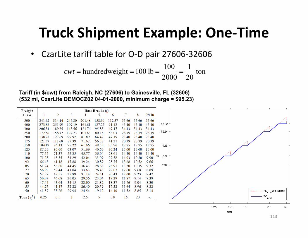
Truck Shipment Example: One‐Time

Tariff (in $/cwt) from Raleigh, NC (27606) to Gainesville, FL (32606) (532 mi, CzarLite DEMOCZ02 04-01-2000, minimum charge = $95.23)

$

• CzarLite tariff table for O‐D pair 27606‐32606 100 1hundredweight 100 lb ton2000 20

cwt

113

Truck Shipment Example: One‐Time9. Using the same LTL shipment, what is the transport cost 

found using the undiscounted CzarLite tariff?

0.8889, 200

0, 95.23

q class

disc MC

1

3 32

3

arg

arg

arg 0.8889 1 30.5

B BBi ii

B BB

B

i q q qq

q q qq

q

tariff 1 max ,min ( , ) 20 , ( , 1) 20

1 0 max 95.23, min (200,3) 20(0.8889), (200,4) 20(1)

max 95.23,min (99.92) 20(0.8889), (81.89)20(1)

max 95.23,min 1,776.23,1,637.80 $1,637.80

Bic disc MC OD class i q OD class i q

OD OD

114

Truck Shipment Example: One‐Time10. What is the implied discount of the estimated charge from 

the CzarLite tariff cost?

tariff

tariff

1,637.80 1,403.401,637.80

14.31%

LTLc cdiscc

0.25 0.5 1 2.5 5ton

638

999

1638

3224

4719

$

TCtariffw/o Break

TCtariff( , 1)( , )

81.89 (1) 0.8196 ton99.92

W Bi i

OD class iq qOD class i

• What is the weightbreak betweenthe rate breaks?

115

Truck Shipment Example: Periodic11. Continuing with the example: assuming a constant annual 

demand for the product of 20 tons, what is the number of full truckloads per year?

max max

20 ton/yr

6.1111 ton/ TL (full truckload )

20 3.2727 TL/yr, average shipment frequency6.1111

f

q q q q

fnq

• Why should this number not be rounded to an integer value?

116

Truck Shipment Example: Periodic12. What is the shipment interval?

1 6.1111 0.3056 yr/TL, average shipment interval20

qtn f

• How many days are there between shipments?

365.25 day/yr

365.25365.25 111.6042 day/TLtn

117

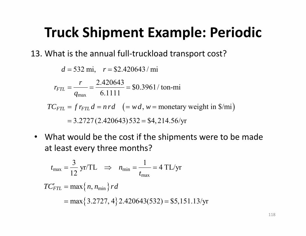
Truck Shipment Example: Periodic13. What is the annual full‐truckload transport cost?

max

532 mi, $2.420643 / mi

2.420643 $0.3961/ ton-mi6.1111

, monetary weight in $/mi

3.2727 (2.420643)532 $4, 214.56/yr

FTL

FTL FTL

d r

rrq

TC f r d n rd wd w

• What would be the cost if the shipments were to be made at least every three months?

max minmax

min

3 1yr/TL 4 TL/yr12

max ,

max 3.2727, 4 2.420643(532) $5,151.13/yr

FTL

t nt

TC n n rd

118

Truck Shipment Example: Periodic• Independent and allocated full‐truckload charges:

131/2000

51

3192

2128

1064

2.45 13.37 26.73

Shipment Size (tons)

Tran

sport C

harge ($)

MC

LTL

1 TL

2 TL

3 TL

Independent

Allocat

ed Ful

l‐Truck

load

Allocat

ed 

Trucklo

ad

Transport Charge for a Shipment

max 0, c ( ), FTLq q UB LB q qr d

119

Truck Shipment Example: Periodic• Total Logistics Cost (TLC) includes all costs that could change 

as a result of a logistics‐related decision

cycle pipeline safety

transport cost

inventory cost

purchase cost

TLC TC IC PC

TC

IC

IC IC IC

PC

• Cycle inventory: held to allow cheaper large shipments• Pipeline inventory: goods in transit or awaiting transshipment• Safety stock: held due to transport uncertainty• Purchase cost: can be different for different suppliers 

120

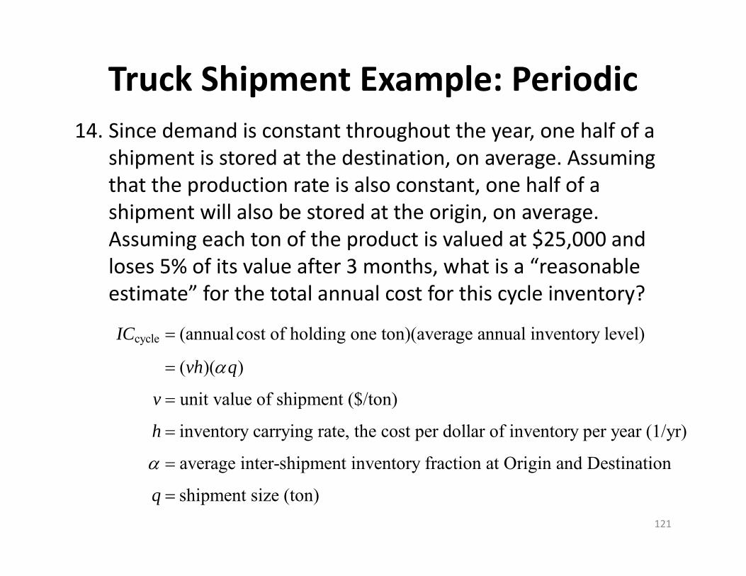
Truck Shipment Example: Periodic14. Since demand is constant throughout the year, one half of a 

shipment is stored at the destination, on average. Assuming that the production rate is also constant, one half of a shipment will also be stored at the origin, on average. Assuming each ton of the product is valued at $25,000 and loses 5% of its value after 3 months, what is a “reasonable estimate” for the total annual cost for this cycle inventory?

cycle (annualcost of holding one ton)(average annual inventory level)

( )( )

unit value of shipment ($/ton)

inventory carrying rate, the cost per dollar of inventory per year (1/yr)

average int

IC

vh q

v

h

er-shipment inventory fraction at Origin and Destination

shipment size (ton)q 121

Truck Shipment Example: Periodic• Rate (h) = sum of interest + warehousing + obsolescence rate• Interest: 5% per Total U.S. Logistics Costs• Warehousing: 6% per Total U.S. Logistics Costs• Obsolescence: default rate hannual = 0.3 hobs 0.2

– Hourly vs Annual: hhour = hannual/H = 0.3/2000 = 0.00015 (H = oper hr/yr)– High FGI cost: h hobs, can ignore interest & warehousing– Estimate hobs using “percent‐reduction interval” method: given time th

when product loses xh‐percent of its original value v, find hobs

– Example: If a product loses 5% of its value after 3 months:

122

obs obs obsobs

, andh hh h h h h

h

x xh t v x v h t x h tt h

obs3 0.050.25 yr 0.2 0.05 0.06 0.2 0.3

12 0.25h

hh

xt h ht

Truck Shipment Example: Periodic• Average annual inventory level

2q

0

q q

2q

0

1 1 (1) 12 2 2 2q q q q

123

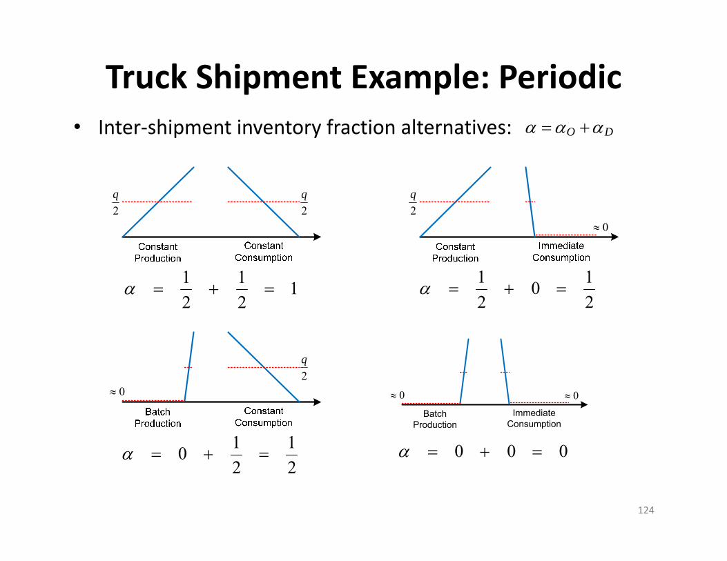
Truck Shipment Example: Periodic• Inter‐shipment inventory fraction alternatives: 

2q

2q

02q

2q

0

Batch Production

Immediate Consumption

0 0

1 1 12 2

1 102 2

1 102 2

0 0 0

O D

124

Truck Shipment Example: Periodic• “Reasonable estimate” for the total annual cost for the 

cycle inventory:

cycle

max

(1)(25,000)(0.3)6.1111

$45,833.33 / yr

where

1 1at Origin + at Destination 12 2$25,000 unit value of shipment ($/ton)

0.3 estimated carrying rate (1/yr)

= 6.111 FTL shipment size (ton

IC vhq

v

h

q q

)

125

Truck Shipment Example: Periodic15. What is the annual total logistics cost (TLC) for these full‐

truckload TL shipments?

cycle

3.2727 (2.420643)532 (1)(25,000)(0.3)6.1111

4, 214.56 45,833.33

$50,047.89 /

FTL FTLTLC TC IC

n rd vhq

yr

126

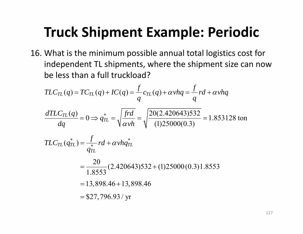
Truck Shipment Example: Periodic16. What is the minimum possible annual total logistics cost for 

independent TL shipments, where the shipment size can now be less than a full truckload?

( ) ( ) ( ) ( )TL TL TLf fTLC q TC q IC q c q vhq rd vhqq q

*( ) 20(2.420643)5320 1.853128 ton(1)25000(0.3)

TLTL

dTLC q frdqdq vh

* **( )

20 (2.420643)532 (1)25000(0.3)1.85531.855313,898.46 13,898.46

$27,796.93 / yr

TL TL TLTL

fTLC q rd vhqq

127

Truck Shipment Example: Periodic• Including the minimum charge and maximum payload 

restrictions:

• What is the TLC if this size shipment could be made as an allocated full‐truckload?

*max

max ,min ,

TLTL

f rd MC frdq qvh vh

128

* * * **

max( )

2.42064320 532 (1)25000(0.3)1.85536.1111

4,214.56 13,898.46

$18,112.82 / yr vs. $27,796.93 as independent P2P TL

AllocFTL TL TL FTL TL TLTL

f rTLC q q r d vhq f d vhqqq

Truck Shipment Example: Periodic17. What is the optimal LTL shipment size?

( ) ( ) ( ) ( )LTL LTL LTLfTLC q TC q IC q c q vhqq

* arg min ( ) 0.725542 tonLTL LTLq

q TLC q

• Must be careful in picking starting point for optimization since

2

1 1527 29

1487 2 142

LTL LTL

s

r PPIs sq d

3150 10,000 , 37 3354, 2000 650 ft2,000 2,000

qq ds

129

Truck Shipment Example: Periodic18. Should the product be shipped TL or LTL?

* * *( ) ( ) ( ) 32,660.43 5, 441.56 $38,102.00 / yrLTL LTL LTL LTL LTLTLC q TC q IC q

0.68 1.86Shipment weight (tons)

27830

35905

$ pe

r yea

r

TLCTL

TLCLTL

TCTL

TCLTL

IC

130

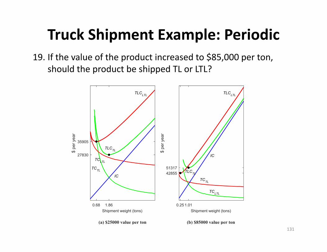
Truck Shipment Example: Periodic19. If the value of the product increased to $85,000 per ton, 

should the product be shipped TL or LTL?

0.68 1.86Shipment weight (tons)

(a) $25000 value per ton

27830

35905

$ pe

r yea

r

TLCTL

TLCLTL

TCTL

TCLTL

IC

0.25 1.01Shipment weight (tons)

(b) $85000 value per ton

4285551317

$ pe

r yea

r

TLCTL

TLCLTL

TCTL

TCLTL

IC

131

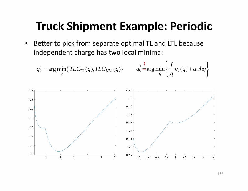
Truck Shipment Example: Periodic• Better to pick from separate optimal TL and LTL because 

independent charge has two local minima:

*0 arg min ( ), ( ) TL LTL

qq TLC q TLC q *

0 0arg min ( )

q

fq c q vhqq

!

132

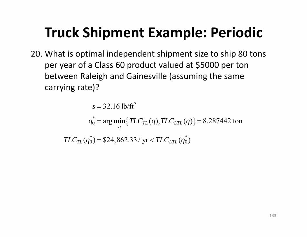
Truck Shipment Example: Periodic20. What is optimal independent shipment size to ship 80 tons 

per year of a Class 60 product valued at $5000 per ton between Raleigh and Gainesville (assuming the same carrying rate)?

133

3

*0

* *0 0

32.16 lb/ft

arg min ( ), ( ) 8.287442 ton

( ) $24,862.33 / yr ( )

TL LTLq

TL LTL

s

q TLC q TLC q

TLC q TLC q

Truck Shipment Example: Periodic21. What is the optimal shipment size if both shipments will 

always be shipped together on the same truck (with same shipment interval)?

1 2 1 2 1 2

agg 1 2

agg 3agg 3 1 2

1 2

1 2agg 1 2

agg agg

, ,

20 80 100 ton

aggregate weight, in lb 100 14.31 lb/ft20 80aggregate cube, in ft4.44 32.16

20 8085,000 5000 $21,000 / ton100 100

d d h h

f f f

fs f f

s s

f fv v vf f

agg*

agg

100(2.3953)532 4.52117 ton(1)21000(0.3)TL

f rdq

v h

134

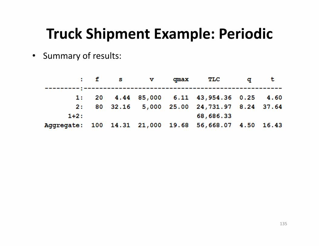
Truck Shipment Example: Periodic• Summary of results:

135

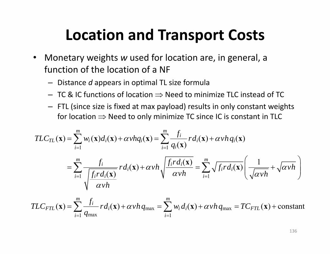
Location and Transport Costs• Monetary weights w used for location are, in general, a 

function of the location of a NF– Distance d appears in optimal TL size formula– TC & IC functions of location  Need to minimize TLC instead of TC– FTL (since size is fixed at max payload) results in only constant weights 

for location  Need to only minimize TC since IC is constant in TLC

136

1 1

1 1

max maxmax1 1

( ) ( ) ( ) ( ) ( ) ( )( )

( ) 1( ) ( )( )

( ) ( ) ( ) ( ) con

m mi

TL i i i i iii i

m mi i i

i i ii ii i

m mi

FTL i i i FTLi i

fTLC w d vhq rd vhqq

f f rdrd vh f rd vhvhf rd vh

vh

fTLC rd vhq w d vhq TCq

x x x x x xx

xx xx

x x x x stant

FTL Location Example• Where should a DC be located in order to minimize 

transportation costs, given:1. FTLs containing mix of products 

A and B shipped P2P from DC to customers in Winston‐Salem, Durham, and Wilmington

2. Each customer receives 20, 30,and 50% of total demand  

3. 100 tons/yr of A shipped FTL P2P to DC from supplier in Asheville 4. 380 tons/yr of B shipped FTL P2P to DC from Statesville5. Each carton of A weighs 30 lb, and occupies 10 ft3

6. Each carton of B weighs 120 lb, and occupies 4 ft3

7. Revenue per loaded truck‐mile is $28. Each truck’s cubic and weight capacity is 2,750 ft3 and 25 tons, 

respectively

137

-83 -82 -81 -80 -79 -78

34

34.5

35

35.5

36

36.5

AshevilleStatesville

Winston-Salem GreensboroDurham

Raleigh

Wilm

ington

50

150

190 220270

295

420

40

FTL Location Example($/yr) ($/mi-yr) (mi)

,($/mi-yr) (TL/yr) ($/TL-mi)(ton/yr) ($/ton-mi)

,($/ton-mi) max max

,

i i

i i FTL i i i

FTL i

TC w d

w f r n r

r fr nq q

in out in out

in out

(Montetary) Weight Losing: 79 67 39 33

Physically Weight Unchanging (DC): 480 480

w w n n

f f

138

Winston-Salem

Statesville

Wilmington

DC 35%

Asheville

Durham

1330 3348 20

78 > 7348 < 73

:iw

*

Asheville DurhamStatesville Winston-Salem Wilmington

146, 732

WW

DC 4

3

5

1

232 max

2 2 2

120 30(2750)30 lb/ft , min 25, 25 ton4 2000

380380, 15.2, 15.2(2) 30.425

s q

f n w

3 agg 3 3

4 agg 4 4

5 agg 5 5

960.20 96, 6.69, 6.69(2) 13.3814.3478

1440.30 144, 10.04, 10.04(2) 20.0714.3478

2400.50 240, 16.73, 16.73(2) 33.4514.3478

f f n w

f f n w

f f n w

31 max

1 1 1

30 3(2750)3 lb/ft , min 25, 4.125 ton10 2000

100100, 24.24, 24.24(2) 48.484.125

s q

f n w

agg 3agg agg max

480 10.4348(2750$2 / TL-mi, 100 380 480 ton/yr, 10.4348 lb/ft , 25, 14.3478100 380 20003 30

A BA B

A B

fr f f f s qf f

s s

FTL Location Example• Include monthly outbound frequency constraint:

– Outbound shipments must occur at least once each month– Implicit means of including inventory costs in location decision

139

max minmax

min

3 3

4 4

5 5

1 1yr/TL 12 TL/yr12

max ,

max 6.69,12 12, 12(2) 24

max 10.04,12 12, 12(2) 24

max 16.73,12 16.73, 16.73(2) 33.45

FTL

t nt

TC n n rd

n w

n w

n w

2430 3348 24

78 < 8048 < 80

:iw

*

Asheville DurhamStatesville Winston-Salem Wilmington

102 > 80160, 80

2WW

in out in out

in out

(Montetary) Weight : 79 81 39 41

Physically Weight Unchanging (DC)

Ga

: 480 48

ining

0

w w n n

f f

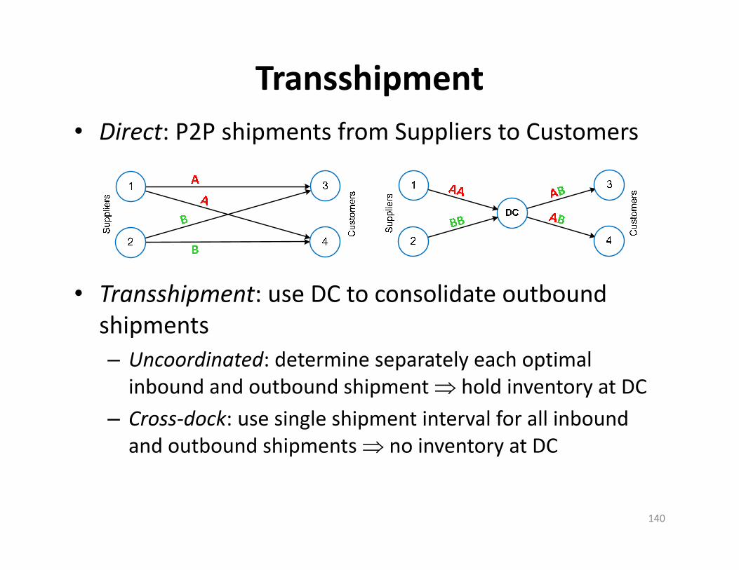
Transshipment• Direct: P2P shipments from Suppliers to Customers

• Transshipment: use DC to consolidate outbound shipments– Uncoordinated: determine separately each optimal inbound and outbound shipment  hold inventory at DC

– Cross‐dock: use single shipment interval for all inbound and outbound shipments  no inventory at DC

140

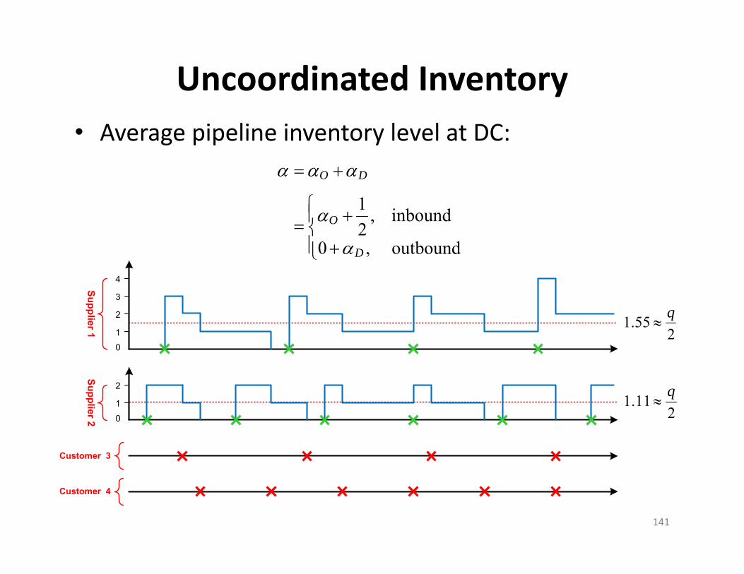
Uncoordinated Inventory • Average pipeline inventory level at DC:

1

2

3

0

4

1

2

0

1.552

q

1.112

q

Supplier 2

Customer 4

Supplier 1

Customer 3

1 , inbound2

0 , outbound

O D

O

D

141

TLC with Transshipment• Uncoordinated:

• Cross‐docking:

*

* *

of supplier/customer

arg min ( )

i

i iq

i i

TLC TLC i

q TLC q

TLC TLC q

0

0

*

* *

, shipment interval

( )( )

( ) independent transport charge as function of

0, inbound0 , outbound

arg min ( )

i

O

D

it

i

qtf

c tTLC t vhf tt

c t t

t TLC t

TLC TLC t142

TLC and Location• TLC should include all logistics‐related costs

TLC can be used as sole objective for network design (incl. location)

• Facility fixed costs, two options:1. Use non‐transport‐related facility costs (mix of top‐down and 

bottom‐up) to estimate fixed costs via linear regression2. For DCs, might assume public warehouses to be used for all DCs

Pay only for time each unit spends in WH No fixed cost at DC

• Transport fixed costs:– Costs that are independent of shipment size (e.g., $/mi vs. $/ton‐mi)

• Costs that make it worthwhile to incur the inventory cost associated with larger shipment sizes in order to spread out the fixed cost

– Main transport fixed cost is the indivisible labor cost for a human driver

• Why many logistics networks (e.g., Walmart, Lowes) designed for all FTL transport

143

Example: Optimal Number DCs for Lowe's• Example of logistics network design using TLC• Lowe’s logistics network (2016):

– Regional DCs (15)– Costal holding facilities– Appliance DCs and Flatbed DCs– Transloading facilities

• Modeling approach:– Focus only on Regional DCs– Mix of top‐down (COGS) and 

bottom‐up (typical load/TL parameters)

– FTL for all inbound and outbound shipments– ALA used to determine TC for given number of DCs– IC = αvhqmax x (number of suppliers x number of DCs + number stores)– Assume uncoordinated DC inventory, no cross‐docking– Ignoring max DC‐to‐store distance constraints, consolidation, etc.

• Determined 9 DCs min TLC (15 DCs 0.87% increase in TLC)144

Topics1. Introduction2. Facility location3. Freight transport

– Exam 1 (take home)

4. Network models5. Routing

– Exam 2 (take home)

6. Warehousing– Final project– Final exam (in class)

145

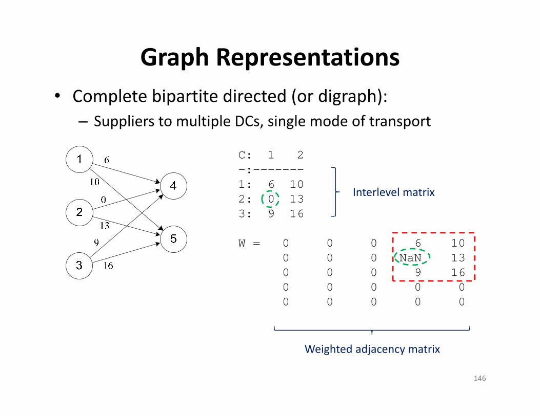
Graph Representations• Complete bipartite directed (or digraph):

– Suppliers to multiple DCs, single mode of transport

C: 1 2-:-------1: 6 102: 0 133: 9 16

W = 0 0 0 6 100 0 0 NaN 130 0 0 9 160 0 0 0 00 0 0 0 0

Interlevel matrix

Weighted adjacency matrix

146

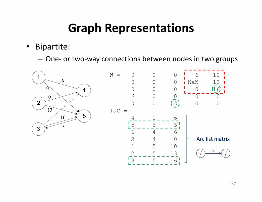
Graph Representations• Bipartite:

– One‐ or two‐way connections between nodes in two groups

Arc list matrix

W = 0 0 0 6 100 0 0 NaN 130 0 0 0 166 0 0 0 00 0 3 0 0

IJC =4 1 65 3 31 4 62 4 01 5 102 5 133 5 16

147

Graph Representations• Multigraph:

– Multiple connections, multiple modes of transport

IJC = 1 -4 61 -4 181 5 102 4 02 5 133 5 163 5 3

no_W =0 0 0 24 100 0 0 NaN 130 0 0 0 1924 0 0 0 00 0 0 0 0

Can’t represent using adjacency matrix148

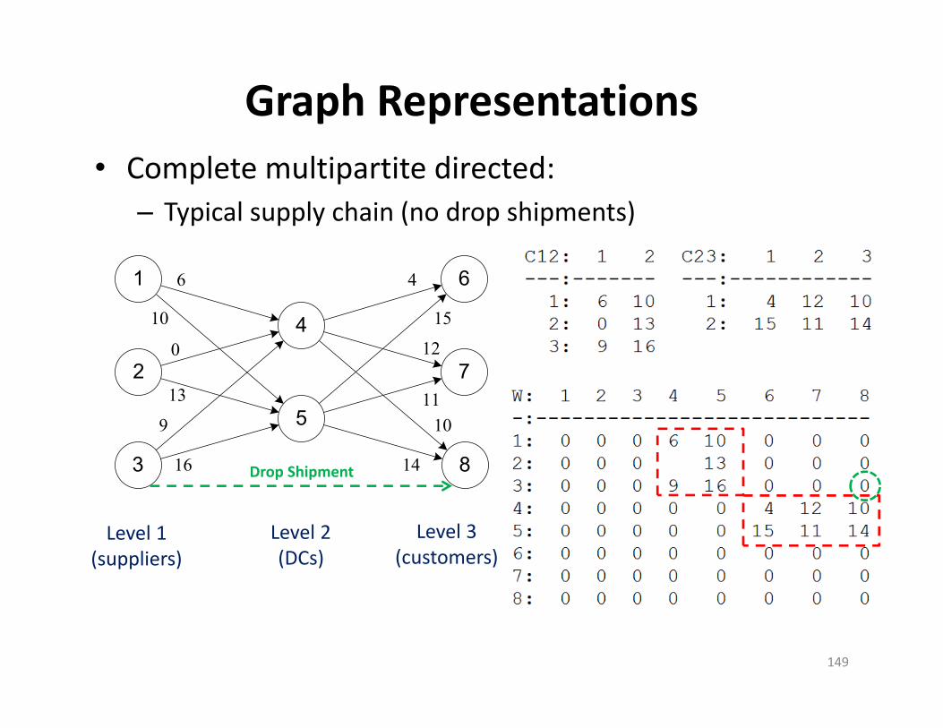
Graph Representations• Complete multipartite directed:

– Typical supply chain (no drop shipments)

Level 1(suppliers)

1

2

4

5

3

12

4

10

15

11

14

6

7

8

10

6

0

13

9

16

Level 2(DCs)

Level 3(customers)

Drop Shipment

149

Transportation Problem• Satisfy node demand from supply nodes

– Can be used for allocation in ALA when NFs have capacity constraints

– Min cost/distance allocation = infinite supply at each node

Trans 4 5 6 7 Supply1 8 6 10 9 552 9 12 13 7 503 14 9 16 5 40

Demand 45 20 30 30

150

Greedy Solution Procedure• Procedure for transportation problem: Continue to select lowest cost supply until all demand is satisfied– Fast, but not always optimal for transportation problem– Dijkstra’s shortest path and simplex method for LP are optimal greedy procedures

Trans 4 5 6 7 Supply1 8 6 10 9 552 9 12 13 7 503 14 9 16 5 40

Demand 45 20 30 30

151

0

‐30 = 10

‐20 = 35

010

‐35 = 0

0

‐10 = 40

0

‐30 = 10

5(30) 6(20) 8(35) 9(10) 13(30) 1, vs 970 optima0 l30TC

Min Cost Network Flow (MCNF) Problem• Most general network problem, can solve using any type of graph representation

MCNF: lhs C C C C C C rhs ----:-------------------------------- Min: 2 3 4 5 1 3 1: 6 1 1 0 0 0 0 6 2: 2 -1 0 1 1 0 0 2 3: 0 0 -1 0 0 1 0 0 4: 0 0 0 -1 0 0 1 0 lb: 0 0 0 0 0 0 ub: Inf Inf Inf Inf Inf Inf

Row for node 5 is redundant

Arc cost: 2 3 4 5 1 3

Net node supply : 6 2 0 0 8

1 1 0 0 0 01 0 1 1 0 0

Incidence Matrix : 0 1 0 0 1 00 0 1 0 0 10 0 0 1 1 1

c

s

A

MCNF: max 's.t.

0

c xAx s

x

net supply of node

0, supply node0, demand node0, transshipment node

is i

152

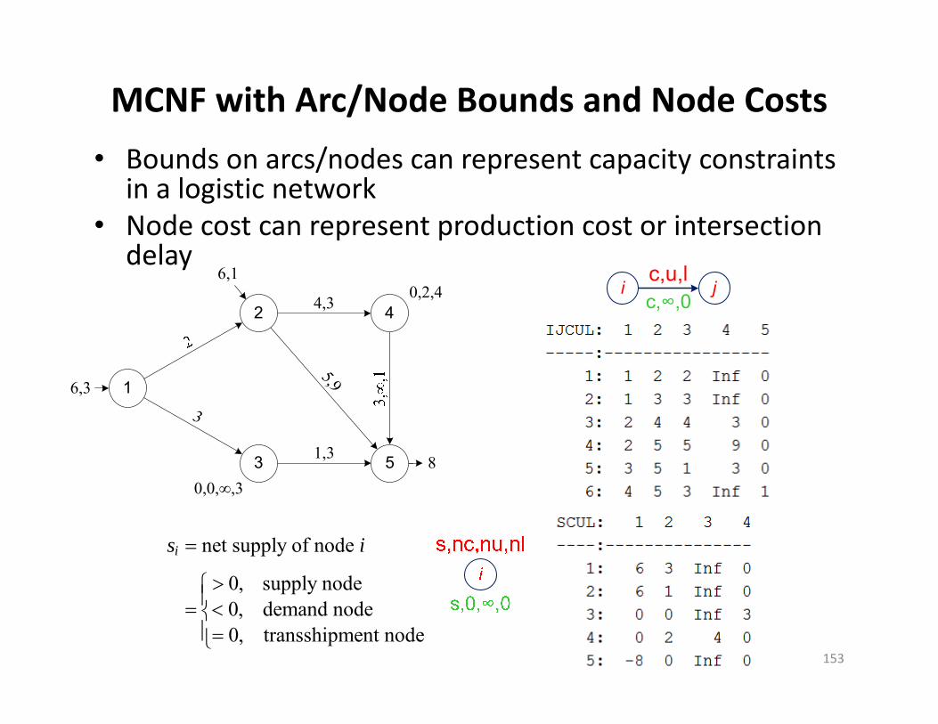
MCNF with Arc/Node Bounds and Node Costs• Bounds on arcs/nodes can represent capacity constraints 

in a logistic network• Node cost can represent production cost or intersection 

delay

net supply of node

0, supply node0, demand node0, transshipment node

is i

4,3

5,9

1,3

3

8

6,3

6,10,2,4

0,0,∞,3

2

3

1

4

5

i jc,∞,0

153

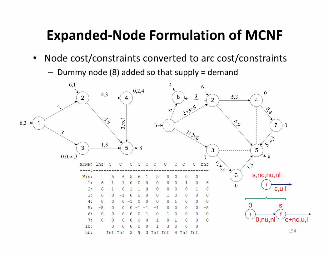
Expanded‐Node Formulation of MCNF• Node cost/constraints converted to arc cost/constraints

– Dummy node (8) added so that supply = demand

4,3

5,9

1,3

3

8

6,3

6,10,2,4

0,0,∞,3

2

3

1

4

5

is,nc,nu,nl

c,u,l

i0

0,nu,nliʹs

c+nc,u,l154

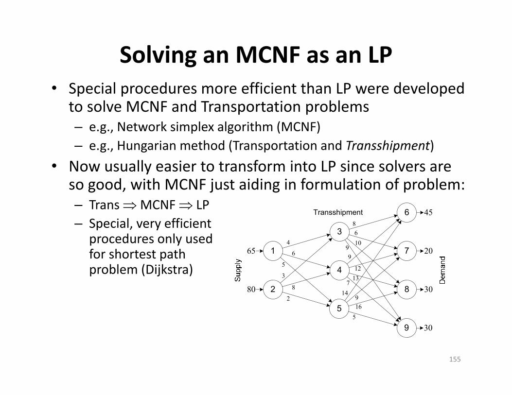
Solving an MCNF as an LP• Special procedures more efficient than LP were developed 

to solve MCNF and Transportation problems– e.g., Network simplex algorithm (MCNF)– e.g., Hungarian method (Transportation and Transshipment)

• Now usually easier to transform into LP since solvers are so good, with MCNF just aiding in formulation of problem:– Trans MCNF LP– Special, very efficient 

procedures only usedfor shortest pathproblem (Dijkstra)

65

80

Transshipment 45

20

30

106

8

99

1213

714

916

5

30

7

6

8

9

4

6

5

3

8

2

3

4

5

1

2

155

Dijkstra Shortest Path Procedure

2

4 6

38 21s t

0,1

4,1

2,1 12,3

10,33,3

14,4

10,4

13,5

Path: 1 3 2 4 5 6 : 13 156

Dijkstra Shortest Path Procedure

4

3

2

2 Simplex (LP)Ellipsoid (LP)Hungarian (transportation)Dijkstra (linear min)

log Dijkstra (Fibonocci heap)no. arcs

nOO nO nO nO m nm

Orderimportant

Index to indexvector nS

157

Other Shortest Path Procedures• Dijkstra requires that all arcs have nonnegative lengths

– Is a “label setting” algorithm since step to final solution made as each node labeled

– Can find longest path (used in CPM) by making by negating arc lengths 

• Networks with some negative arcs require slower “label correcting” procedures that repeatedly check for optimality at all nodes or detect a negative cycle– Negative arcs used in project scheduling to represent maximum 

lags between activities• A* algorithm adds to Dijkstra an heuristic estimate of 

each node’s remaining distance to destination– Used in AI search for all types of applications (tic‐tac‐toe, chess)– In path planning applications, great circle distance from each 

node to destination could be used as estimate of remaining distance

158

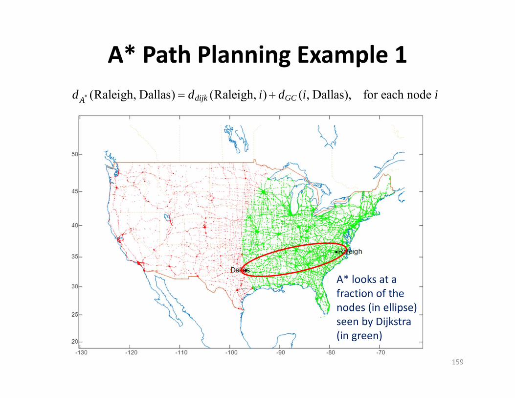
A* Path Planning Example 1

159

* (Raleigh, Dallas) (Raleigh, ) ( , Dallas), for each node dijk GCAd d i d i i

A* looks at a fraction of the nodes (in ellipse) seen by Dijkstra  (in green)

A* Path Planning Example 2• 3‐D (x,y,t) A* used for planning path of each container in a DC

• Each container assigned unique priority that determines planning sequence – Paths of higher‐priority containers become obstacles for subsequent containers

160

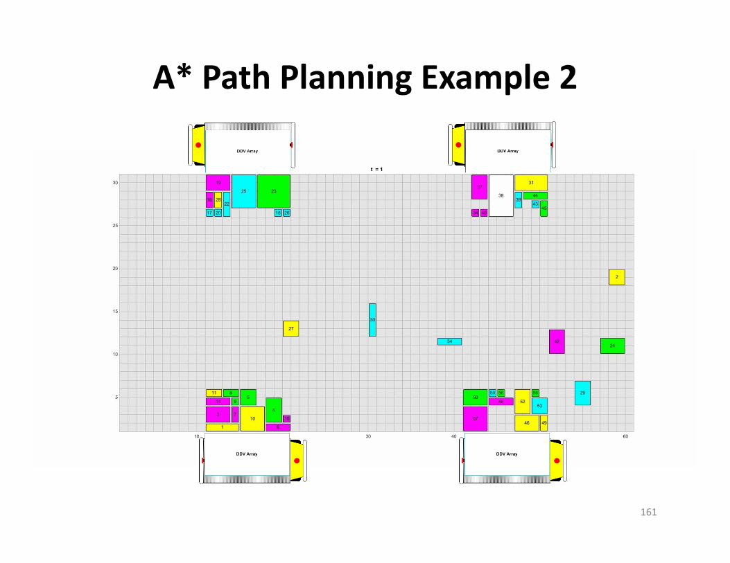
A* Path Planning Example 2

161

Minimum Spanning Tree• Find the minimum cost set of arcs that connect all nodes– Undirected arcs: Kruskal’s algorithm (easy to code)– Directed arcs: Edmond’s branching algorithm (hard to code)

162

1

2

3

4

5

6

7

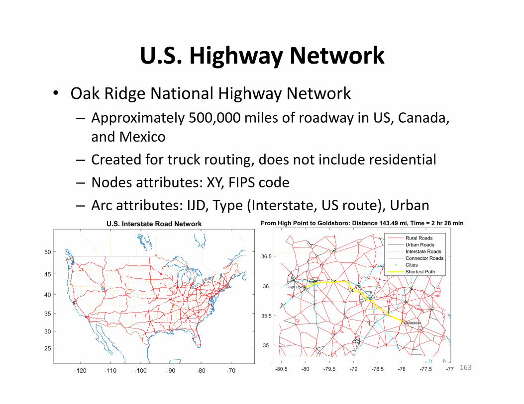
U.S. Highway Network• Oak Ridge National Highway Network

– Approximately 500,000 miles of roadway in US, Canada, and Mexico

– Created for truck routing, does not include residential– Nodes attributes: XY, FIPS code– Arc attributes: IJD, Type (Interstate, US route), Urban

163-80.5 -80 -79.5 -79 -78.5 -78 -77.5 -77

35

35.5

36

36.5

From High Point to Goldsboro: Distance 143.49 mi, Time = 2 hr 28 min

High Point

Goldsboro

Rural RoadsUrban RoadsInterstate RoadsConnector RoadsCitiesShortest Path

-120 -110 -100 -90 -80 -70

25

30

35

40

45

50

U.S. Interstate Road Network

FIPS Codes• Federal Information Processing Standard (FIPS) codes used to 

uniquely identify states (2‐digit) and counties (3‐digit)– 5‐digit Wake county code = 2‐digit state + 3‐digit county= 37183 = 37 NC FIPS + 183 Wake FIPS

164

Road Network Modifications1. Thin

– Remove all degree‐2 nodes from network– Add cost of both arcs incident to each degree‐2 node– If results in multiple arcsbetween pair of nodes, keepminimum cost

165

Thinned I‐40 Around Raleigh

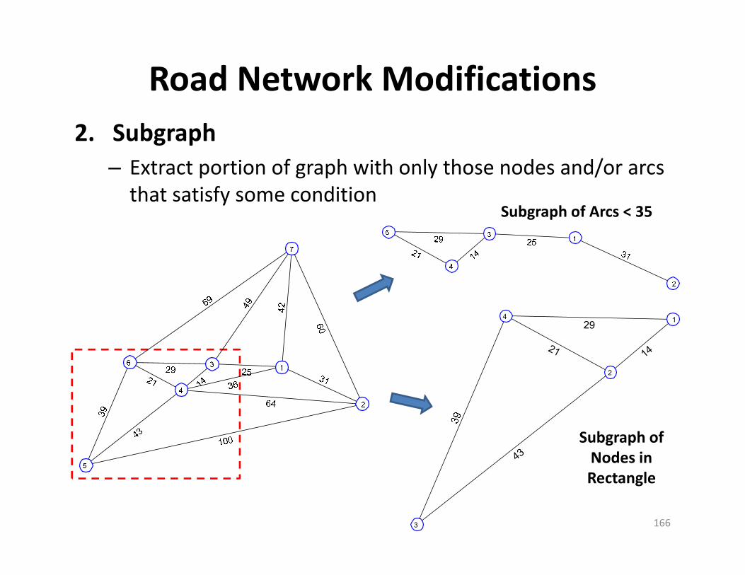
Road Network Modifications2. Subgraph

– Extract portion of graph with only those nodes and/or arcs that satisfy some condition

166

Subgraph of Arcs < 35

14

43

29

21

1

2

3

4

Subgraph of Nodes in Rectangle

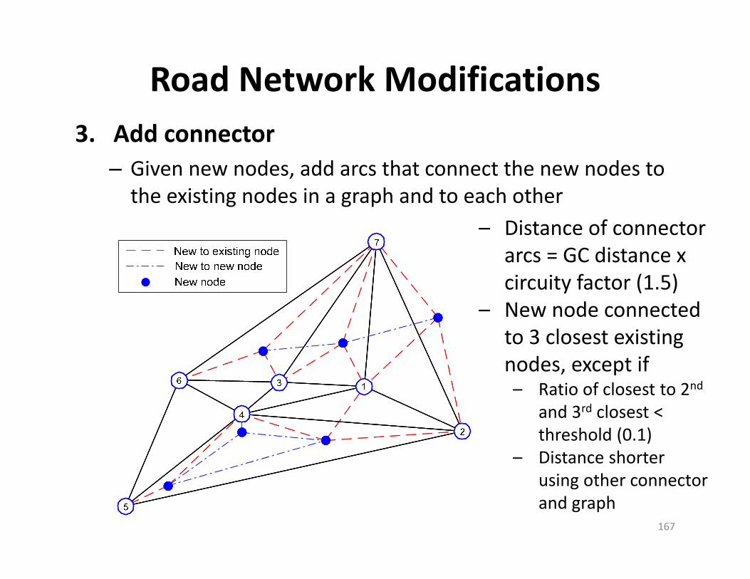
Road Network Modifications3. Add connector

– Given new nodes, add arcs that connect the new nodes to the existing nodes in a graph and to each other

167

– Distance of connector arcs = GC distance x circuity factor (1.5)

– New node connected to 3 closest existing nodes, except if– Ratio of closest to 2nd

and 3rd closest < threshold (0.1)

– Distance shorter using other connector and graph

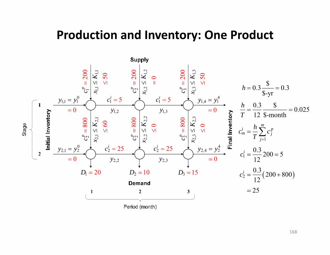
Production and Inventory: One Product

168

1

1

2

$0.3 0.3$-yr

0.3 $ 0.02512 $-month

0.3 200 5120.3 200 8001225

mi pm j

j

i

i

h

hT

hc cT

c

c

280

0p c

01,1 1

0y y

120

0p c

1

1,2

5icy

1 20D

02,1 2

0y y

220

0p c

2

2,2

25icy

2 10D

1

1,3

5icy

320

0p c

2

2,3

25icy

3 15D

41,4 1

0y y

42,4 2

0y y

1,11,1

50x

K

1,2

1,2

0x

K

1,3

1,3

50x

K

2,1

2,1

60x

K

280

0p c

2,2

2,2

0x

K

280

0p c

2,3

2,3

0x

K

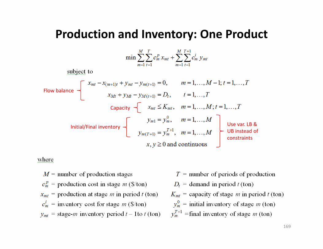
Production and Inventory: One Product

169

Flow balance

Initial/Final inventory

Capacity

Use var. LB & UB instead of constraints

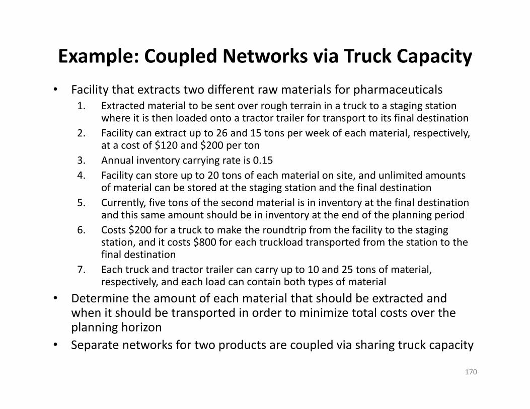
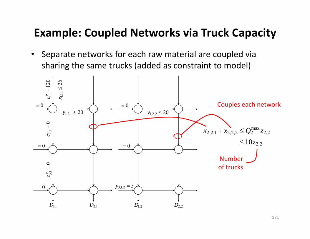
Example: Coupled Networks via Truck Capacity• Facility that extracts two different raw materials for pharmaceuticals

1. Extracted material to be sent over rough terrain in a truck to a staging station where it is then loaded onto a tractor trailer for transport to its final destination

2. Facility can extract up to 26 and 15 tons per week of each material, respectively, at a cost of $120 and $200 per ton

3. Annual inventory carrying rate is 0.154. Facility can store up to 20 tons of each material on site, and unlimited amounts 

of material can be stored at the staging station and the final destination5. Currently, five tons of the second material is in inventory at the final destination 

and this same amount should be in inventory at the end of the planning period6. Costs $200 for a truck to make the roundtrip from the facility to the staging 

station, and it costs $800 for each truckload transported from the station to the final destination

7. Each truck and tractor trailer can carry up to 10 and 25 tons of material, respectively, and each load can contain both types of material

• Determine the amount of each material that should be extracted and when it should be transported in order to minimize total costs over the planning horizon

• Separate networks for two products are coupled via sharing truck capacity

170

Example: Coupled Networks via Truck Capacity

• Separate networks for each raw material are coupled via sharing the same trucks (added as constraint to model)

171

max2,2,1 2,2,2 2 2,2

2,210x x Q z

z

Couples each network

Numberof trucks

2,1

0p c

1,112

0p c

1,2,1 20y

1,1D 2,1D

1,1,1

26x

3,1

0p c

0

0

0

1,2,2 20y

1,2D 2,2D

0

0

3,1,2 5y

Example: Coupled Networks via Truck Capacity

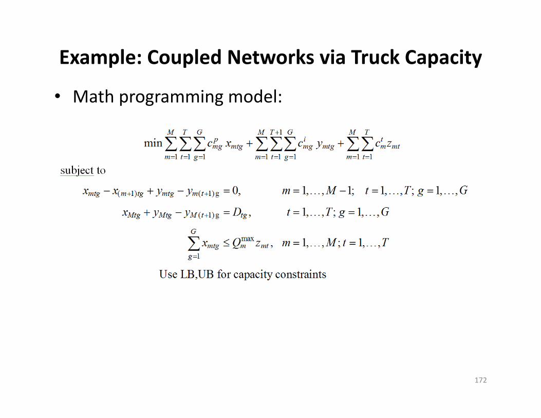
• Math programming model:

172

Production and Inventory: Multiple Products

173

pc ic

0

0

sc 0

0

0

pc ic sc 0

1k 2k 1

0

0

Prod

uct 1

Prod

uct 2

Production and Inventory: Multiple Products

174

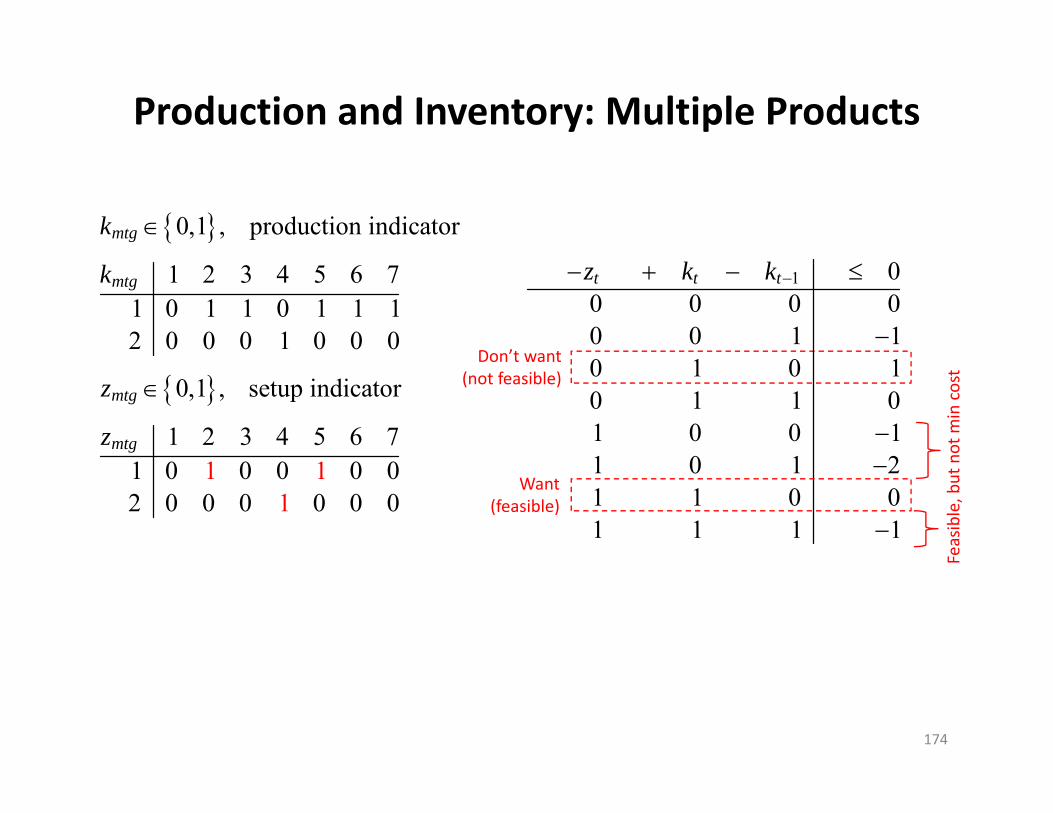
0,1 , production indicator

1 2 3 4 5 6 71 0 1 1 0 1 1 12 0 0 0 1 0 0 0

0,1 , setup indicator

1 2 3 4 5 6 71 0 0 0 0 02 0 0 0 0

11 0

10

mtg

mtg

mtg

mtg

k

k

z

z

Don’t want

(not feasible)

Want(feasible)

Feasible, b

ut not m

in cost

1 00 0 0 00 0 1 10 1 0 10 1 1 01 0 0 11 0 1 21 1 0 01 1 1 1

t t tz k k

Production and Inventory: Multiple Products

175

Flowbalance

Capacity

Setup

Linking

MILP

dummy

Production and Inventory: Multiple Products

176

Example of Logistics Software Stack

177

• Flow: Data→ Model→ Solver→ Output→ Report– reports are run on a regular period‐to‐period, rolling‐horizon

basis as part of normal operations management– model only changed when logistics network changes

MIP Solver(Gurobi,Cplex,etc.)

Standard Library(in compiled C,Java)

User Library(in script language)

MIP Solver(Gurobi, etc.)

Standard Library(C,Java)

Data(csv,Excel,etc.)

Report(GUI,web,etc.)

CommercialSoftware

(Lamasoft,etc.)

Scripting(Python,Matlab,etc.)

Topics1. Introduction2. Facility location3. Freight transport

– Midterm exam

4. Network models5. Routing6. Warehousing

– Final project– Final exam

178

Routing Alternatives

179

P DPickup Delivery

P D D D

P P P D

P P P DD D

(a) Point-to-point (P2P)

(b) Peddling (one-to-many)

(c) Collecting (many-to-one)

(d) Many-to-many

P D P DP D

(e) Interleaved

P D P D P Dempty

(f) Multiple routes

TSP and VRP

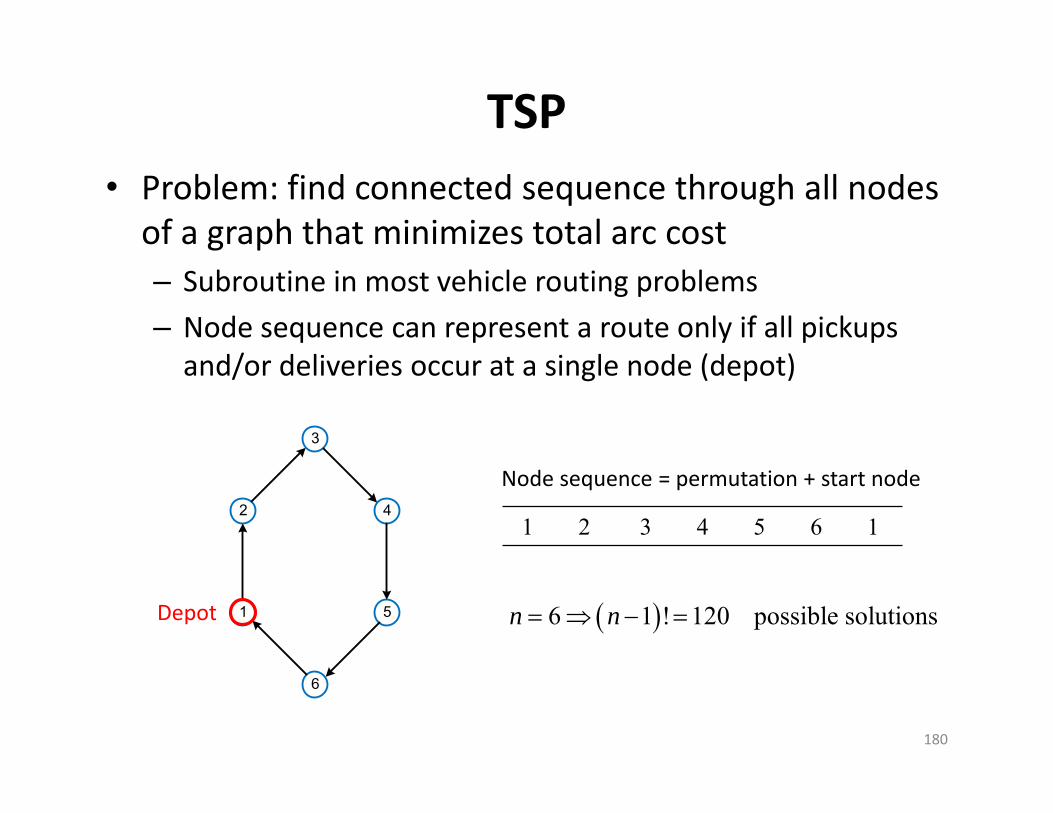
TSP• Problem: find connected sequence through all nodes of a graph that minimizes total arc cost– Subroutine in most vehicle routing problems– Node sequence can represent a route only if all pickups and/or deliveries occur at a single node (depot)

180

1

2

3

4

5

6

1 2 3 4 5 6 1

Node sequence = permutation + start node

Depot 6 1 ! 120 possible solutionsn n

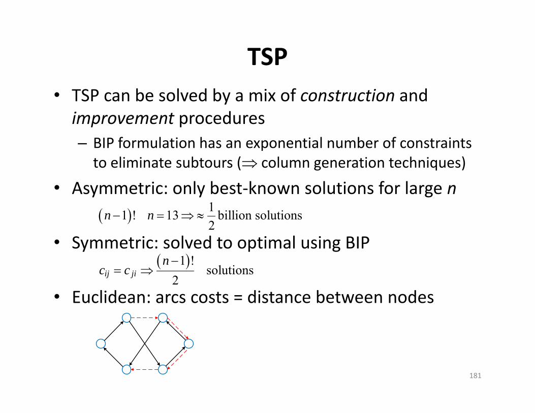
TSP• TSP can be solved by a mix of construction and improvement procedures– BIP formulation has an exponential number of constraints to eliminate subtours ( column generation techniques)

• Asymmetric: only best‐known solutions for large n

• Symmetric: solved to optimal using BIP

• Euclidean: arcs costs = distance between nodes 

181

11 ! 13 billion solutions2

n n

1 !solutions

2ij jin

c c

TSP Construction• Construction easy since any permutation is feasible and can then be improved

182

1 2 3 4 5 6

1 2 4 5 6

1 2 4 6

2 4 6

2 4

2

4

2

3

5

1

6

Spacefilling Curve

183

1.0 0.250 0.254 0.265 0.298 0.309 0.438 0.441 0.452 0.485 0.496 0.500

0.9 0.246 0.257 0.271 0.292 0.305 0.434 0.445 0.458 0.479 0.493 0.504

0.8 0.235 0.229 0.279 0.283 0.333 0.423 0.417 0.467 0.471 0.521 0.515

0.7 0.202 0.208 0.158 0.154 0.354 0.390 0.396 0.596 0.592 0.542 0.548

0.6 0.191 0.180 0.167 0.146 0.132 0.379 0.618 0.604 0.583 0.570 0.559

0.5 0.188 0.184 0.173 0.140 0.129 0.375 0.621 0.610 0.577 0.566 0.563

0.4 0.059 0.070 0.083 0.104 0.118 0.871 0.632 0.646 0.667 0.680 0.691

0.3 0.048 0.042 0.092 0.096 0.896 0.860 0.854 0.654 0.658 0.708 0.702

0.2 0.015 0.021 0.971 0.967 0.917 0.827 0.833 0.783 0.779 0.729 0.735

0.1 0.004 0.993 0.979 0.958 0.945 0.816 0.805 0.792 0.771 0.757 0.746

0.0 0.000 0.996 0.985 0.952 0.941 0.813 0.809 0.798 0.765 0.754 0.750

0.0 0.1 0.2 0.3 0.4 0.5 0.6 0.7 0.8 0.9 1.0

2: 0.0213: 0.1541: 0.4714: 0.783

Sequence determined by sorting position along 1‐D line covering 2‐D space

Two‐Opt Improvement

1 2 3 4 5 6 1

184

a b c d e f

a‐c 1 3 2 4 5 6 1

a‐d 1 4 3 2 5 6 1

a‐e 1 5 4 3 2 6 1

b‐db‐eb‐fc‐ec‐fd‐f

arcs to 2first arc

1 2

3 2 2

3Sequences considered at end to verify local optimum: nodes (1) (1) 9 for 6

2

b nan n n

j i j i

n nn n

TSP Comparison

TSP Procedure Total Cost

1 Spacefilling curve 482.7110

2 1 + 2‐opt 456

3 Convex hull insert + 2‐opt 452

4 Nearest neighbor + 2‐opt 439.6

5 Random construction + 2‐opt 450, 456

6 Eil51 in TSPLIB 426* optimal

185

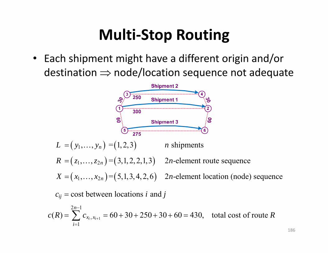
Multi‐Stop Routing• Each shipment might have a different origin and/or destination  node/location sequence not adequate

186

1

1 2

1 2

, , = 1, 2,3 shipments

, , = 3,1, 2, 2,1,3 2 -element route sequence

, , = 5,1,3,4, 2,6 2 -element location (node) sequence

n

n

n

L y y n

R z z n

X x x n

1

2 1

,1

cost of route

cost between locations and

( ) 60 30 250 30 60 430, total i i

ij

n

x xi

c i j

c R Rc

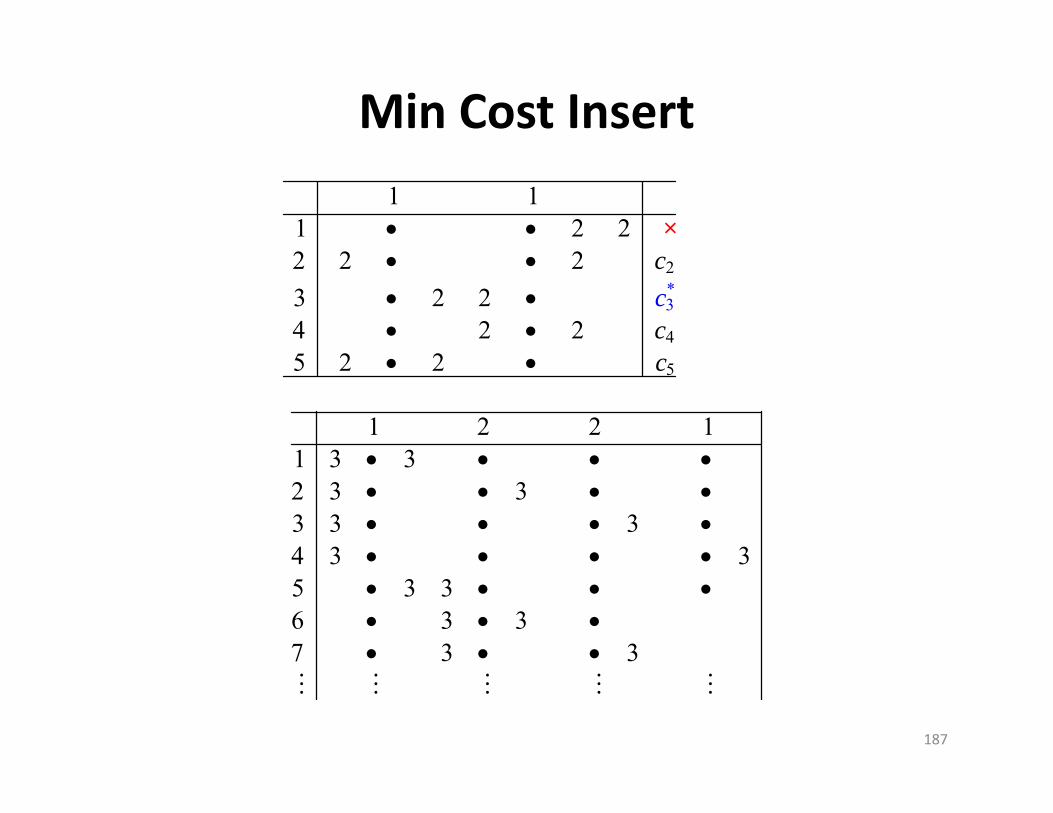
Min Cost Insert

187

*3

2

4

5

1 11 2 22 2 23 2 24 2 25 2 2

c

cc

c

×

1 2 2 11 3 32 3 33 3 34 3 35 3 36 3 37 3 3

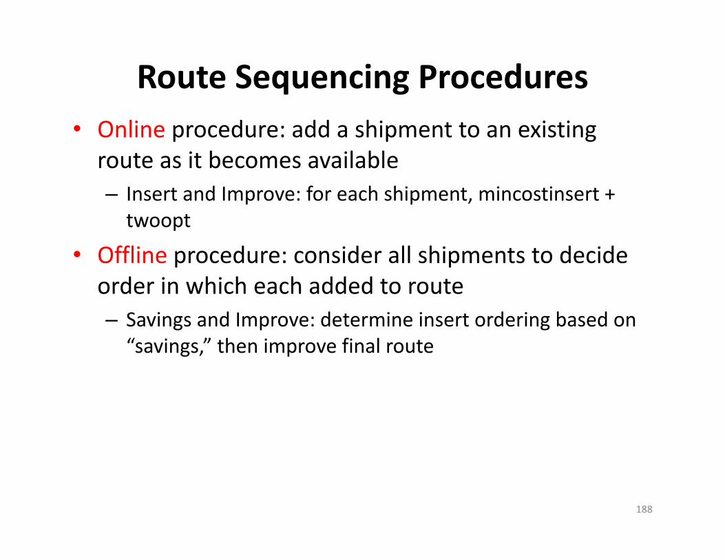
Route Sequencing Procedures• Online procedure: add a shipment to an existing route as it becomes available– Insert and Improve: for each shipment, mincostinsert + twoopt

• Offline procedure: consider all shipments to decide order in which each added to route– Savings and Improve: determine insert ordering based on “savings,” then improve final route

188

Insert and Improve Online Procedure

189

5‐Shipment Example

190

= 3,2,5,5,1, 4,3,1,2,4

= 4,3,7,1,1,6,5,2, 2, 2

R

X

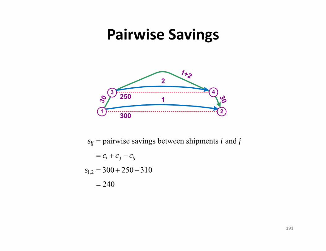
Pairwise Savings

191

1,2

pairwise savings between shipments and

300 250 310

240

ij

i j ij

s i j

c c c

s

300

4

2

250

23

1

1

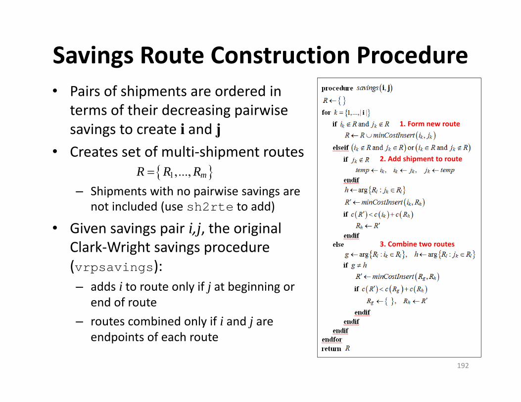
Savings Route Construction Procedure

192

• Pairs of shipments are ordered in terms of their decreasing pairwise savings to create i and j

• Creates set of multi‐shipment routes

– Shipments with no pairwise savings are not included (use sh2rte to add)

• Given savings pair i,j, the original Clark‐Wright savings procedure (vrpsavings):– adds i to route only if j at beginning or 

end of route– routes combined only if i and j are 

endpoints of each route

1,..., mR R R

1. Form new route

2. Add shipment to route

3. Combine two routes

Vehicle Routing Problem• VRP = TSP + vehicle constraints• Constraints:

– Capacity (weight, cube, etc.)– Maximum TC (HOS: 11 hr max)– Time windows (with/without delay at customer)

• VRP uses absolute windows that can be checked by simple scanning• Project scheduling uses relative windows solved by shortest path with 

negative arcs

– Maximum number of routes/vehicles (hard)

• Criteria:1. Number of routes/vehicles2. TC

193

Time Window Example[0,24] hr; Loading/unloading  me = 0; Capacity = ∞; LB = 5 hr

194

(return window)

(depart window)

(earliest start) a = 6

a = 7 – 8 (arrive at 7 wait to 8)

a = 10 – 12

a = 13 – 15

a = 16 – 18

Earliest Finish – Latest Start = 18 – 10 = 8 hr = 5 travel + 3 delay

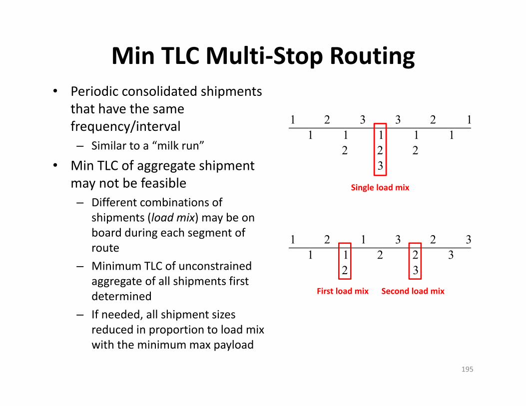
Min TLC Multi‐Stop Routing

195

1 2 3 3 2 11 1 1 1 1

2 2 23

1 2 1 3 2 31 1 2 2 3

2 3

Single load mix

First load mix Second load mix

• Periodic consolidated shipments that have the same frequency/interval– Similar to a “milk run”

• Min TLC of aggregate shipment may not be feasible– Different combinations of 

shipments (load mix) may be on board during each segment of route

– Minimum TLC of unconstrained aggregate of all shipments first determined

– If needed, all shipment sizes reduced in proportion to load mix with the minimum max payload

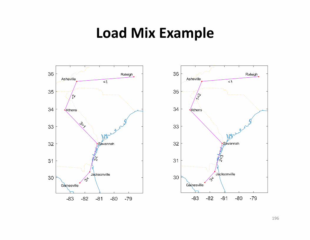
Load Mix Example

196

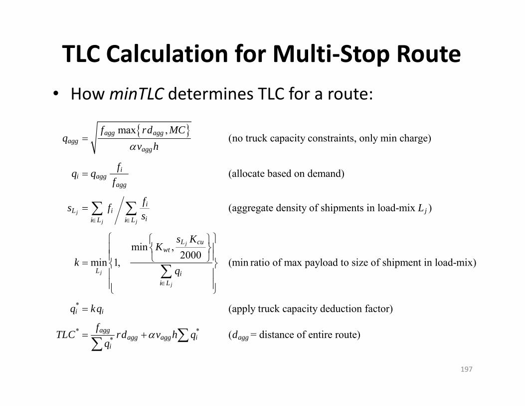
TLC Calculation for Multi‐Stop Route• How minTLC determines TLC for a route:

197

max ,(no truck capacity constraints, only min charge)

(allocate based on demand)

(aggregate density of shipments in load-mix )

min ,min 1,

j

j j

j

j

agg aggagg

agg

ii agg

agg

iL i j

ii L i L

Lwt

L

f rd MCq

v h

fq qf

fs f Ls

s KK

k

*

* **

2000(min ratio of max payload to size of shipment in load-mix)

(apply truck capacity deduction factor)

( = distance of entire route)

j

cu

ii L

i i

aggagg agg i agg

i

q

q kq

fTLC rd v h q d

q

Cost Allocation for Routing

198

Shmt 2

Shmt 1

1+2

600 ft 800 ft 1,200 ft

Cost Allocation for Routing

199

300

4

2

250

23

1

1

6275

35

Shapley Value

200

sav 0

1

n

L i Li

c c c

sav 0 0

,ij i j i jc c c c

{ }

0 1 \| |

! 1 !!i M i M

m n M N iM m

m n mn

sav savsavsav sav

1 1 1

1 11 2 1

n n nij jiL

i jkj j k

c ccc cn n n n

Topics1. Introduction2. Facility location3. Freight transport

– Midterm exam

4. Network models5. Routing6. Warehousing

– Final project– Final exam

201

Warehousing• Warehousing are the activities involved in the design and 

operation of warehouses• A warehouse is the point in the supply chain where raw 

materials, work‐in‐process (WIP), or finished goods are stored for varying lengths of time.

• Warehouses can be used to add value to a supply chain in two basic ways:1. Storage. Allows product to be available where and when its needed.

2. Transport Economies. Allows product to be collected, sorted, and distributed efficiently.

• A public warehouse is a business that rents storage space to other firms on a month‐to‐month basis. They are often used by firms to supplement their own private warehouses.

202

Types of Warehouses

Warehouse Design Process• The objectives for warehouse design can include:

– maximizing cube utilization– minimizing total storage costs (including building, equipment, and labor costs)

– achieving the required storage throughput– enabling efficient order picking

• In planning a storage layout: either a storage layout is required to fit into an existing facility, or the facility will be designed to accommodate the storage layout.

Warehouse Design Elements• The design of a new warehouse includes the 

following elements:1. Determining the layout of the storage locations (i.e., the 

warehouse layout).2. Determining the number and location of the 

input/output (I/O) ports (e.g., the shipping/receiving docks).

3. Assigning items (stock‐keeping units or SKUs) to storage locations (slots).

• A typical objective in warehouse design is to minimize the overall storage cost while providing the required levels of service.

Design Trade‐Off• Warehouse design involves the trade‐off between building and handling costs:

206

min Building Costs vs. min Handling Costs

max Cube Utilization vs. max Material Accessibility

Shape Trade‐Off

207

vs.

Square shape minimizes perimeter length for a given area, thus minimizing building costs

Aspect ratio of 2 (W = 2D) min. expected distance from I/O port to slots, thus minimizing handling costs

Storage Trade‐Off

208

vs.

Maximizes cube utilization, but minimizes material accessibility

Making at least one unit of each item accessible decreases cube utilization

A

A

B

B

B

C

C

D

E

A

A

B

B

B C

C D E

Honeycombloss

Storage Policies• A storage policy determines how the slots in a storage region are assigned to the different SKUs to the stored in the region.

• The differences between storage polices illustrate the trade‐off between minimizing building cost and minimizing handling cost.

• Type of policies:– Dedicated– Randomized– Class‐based

209

Dedicated Storage• Each SKU has a 

predetermined number of slots assigned to it.

• Total capacity of the slots assigned to each SKU must equal the storage space corresponding to the maximum inventory level of each individual SKU.

• Minimizes handling cost.• Maximizes building cost.

210

I/O

A

BC C

Randomized Storage• Each SKU can be stored in 

any available slot.• Total capacity of all the 

slots must equal the storage space corresponding to the maximum aggregateinventory level of all of the SKUs.

• Maximizes handling cost.  • Minimizes building cost.

211

I/O

ABC

Class‐based Storage

A

BC

I/O

212

• Combination of dedicated and randomized storage, where each SKU is assigned to one of several different storage classes.

• Randomized storage is used for each SKU within a class, and dedicated storage is used between classes.

• Building and handling costs between dedicated and randomized.

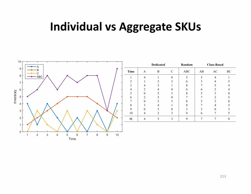
Individual vs Aggregate SKUs

213

Time1 2 3 4 5 6 7 8 9 10

0

1

2

3

4

5

6

7

8

9

10

ABCABC

Dedicated Random Class-Based

Time A B C ABC AB AC BC

1 4 1 0 5 5 4 1 2 1 2 3 6 3 4 5 3 4 3 1 8 7 5 4 4 2 4 0 6 6 2 4 5 0 5 3 8 5 3 8 6 2 5 0 7 7 2 5 7 0 5 3 8 5 3 8 8 3 4 1 8 7 4 5 9 0 3 0 3 3 0 3

10 4 2 3 9 6 7 5

Mi 4 5 3 9 7 7 8

Cube Utilization• Cube utilization is percentage of the total space (or “cube”) 

required for storage actually occupied by items being stored.• There is usually a trade‐off between cube utilization and 

material accessibility.• Bulk storage using block stacking can result in the minimum 

cost of storage, but material accessibility is low since only the top of the front stack is accessible.

• Storage racks are used when support and/or material accessibility is required.

214

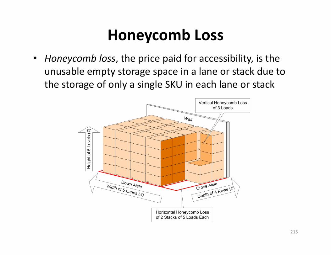
Honeycomb Loss• Honeycomb loss, the price paid for accessibility, is the 

unusable empty storage space in a lane or stack due to the storage of only a single SKU in each lane or stack

215

Hei

ght o

f 5 L

evel

s (Z

)

Wall

Depth of 4 Rows (Y)Cross Aisle

Vertical Honeycomb Lossof 3 Loads

Width of 5 Lanes (X)

Down Aisle

Horizontal Honeycomb Lossof 2 Stacks of 5 Loads Each

Estimating Cube Utilization• The (3‐D) cube utilization for dedicated and randomized 

storage can estimated as follows:

216

1

1

item space item spaceCube utilization honeycomb down aisletotal space item space loss space

, dedicated( )(3-D)

, randomized( )

, dedicated( )(2-D)

Nii

N ii

x y z MTS DCU

x y z MTS D

Mx yH

TA DCUx

, randomized( )

MyH

TA D

Unit Load• Unit load: single unit of an item, or multiple units 

restricted to maintain their integrity• Linear dimensions of a unit load:

• Pallet height (5 in.) + load height gives z: 

217

Depth (stringer length) Width (deckboard length)

(Stringer length) Depth Width (Deckboard length)

x

Deckboards Stringer

Notch

y x

y x z

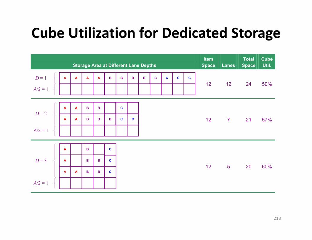
Cube Utilization for Dedicated Storage

Storage Area at Different Lane Depths Item

Space

Lanes Total Space

Cube Util.

A A A A C C CB B B B BD = 1

A/2 = 1

12 12 24 50%

A A C CB B B

A/2 = 1

A A CB B

D = 2

12 7 21 57%

A A CB B

A/2 = 1

A CB BD = 3

A CB

12 5 20 60%

218

Total Space/Area• The total space required, as a function of lane depth D:

219

Eff. lane depth

Total space (3-D): ( ) ( )2 2A ATS D X Y Z xL D yD zH

eff( )Total area (2-D): ( ) ( )2

TS D ATA D X Y xL D yDZ

A

A

x

A A B

B

B

B

B

C

C

C

X = xL

Down Aisle Space

Storage Area on OppositeSide of the Aisle

Number of Lanes• Given D, estimated total number of lanes in region:

• Estimated HCL:

220

1, dedicated

Number of lanes: ( ) 1 1, randomized ( 1)2 2

Ni

i

MDH

L D D HM NH N NDH

1

1

11 1 1 1 12 1 1 2 12 2

D

i

D D DD D iD D D D

1

0

D

1

2

D

D

1

1

D

D

3D

Optimal Lane Depth• Solving for D in                             results in:

221

* 2 1Optimal lane depth for randomized storage (in rows):2 2

A M ND

NyH

0

10,000

20,000

30,000

40,000

50,000

60,000

70,000

Lane D ep t h ( in R o ws)

Item Space 24,000 24,000 24,000 24,000 24,000 24,000 24,000 24,000 24,000 24,000

Honeycomb Loss 1,536 3,648 5,376 7,488 9,600 11,712 13,632 15,936 17,472 20,160

Aisle Space 38,304 20,736 14,688 11,808 10,080 8,928 8,064 7,488 6,912 6,624

Total Space 63,840 48,384 44,064 43,296 43,680 44,640 45,696 47,424 48,384 50,784

1 2 3 4 5 6 7 8 9 10

( ) 0dTS D dD

Max Aggregate Inventory Level• Usually can determine max inventory level for each SKU:

– Mi = maximum number of units of SKU i

• Since usually don’t know M directly, but can estimate it if– SKUs’ inventory levels are uncorrelated– Units of each item are either stored or retrieved at a constant 

rate

• Can add include safety stock for each item, SSi– For example, if the order size of three SKUs is 50 units and 5 units of 

each item are held as safety stock

222

1

12 2

Ni

i

MM

1

1 50 13 5 902 2 2 2

Ni i

ii

M SSM SS

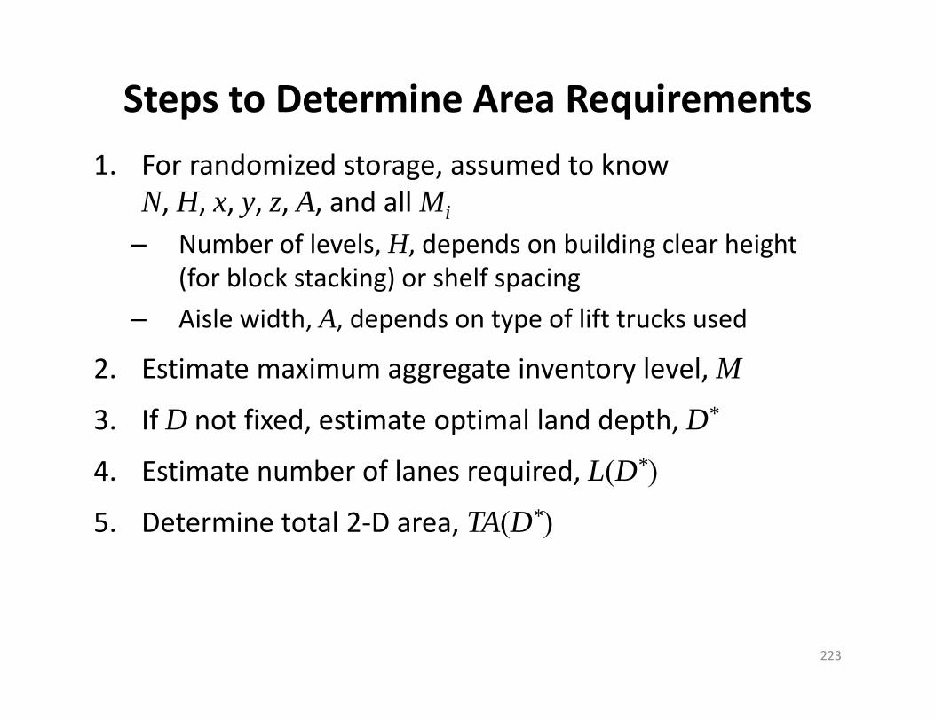
Steps to Determine Area Requirements1. For randomized storage, assumed to know

N, H, x, y, z, A, and all Mi

– Number of levels, H, depends on building clear height (for block stacking) or shelf spacing

– Aisle width, A, depends on type of lift trucks used

2. Estimate maximum aggregate inventory level, M

3. If D not fixed, estimate optimal land depth, D*

4. Estimate number of lanes required, L(D*)

5. Determine total 2‐D area, TA(D*)

223

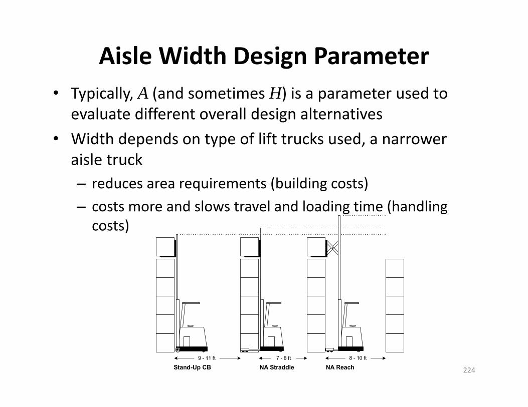
Aisle Width Design Parameter• Typically, A (and sometimes H) is a parameter used to 

evaluate different overall design alternatives• Width depends on type of lift trucks used, a narrower 

aisle truck– reduces area requirements (building costs)– costs more and slows travel and loading time (handling costs)

224

9 - 11 ft 7 - 8 ft 8 - 10 ft

Stand-Up CB NA Straddle NA Reach

Example 1: Area RequirementsUnits of items A, B, and C are all received and stored as 42 36 36 in. (y x z) pallet loads in a storage region that is along one side of a 10‐foot‐wide down aisle in the warehouse of a factory. The shipment size received for each item is 31, 62, and 42 pallets, respectively. Pallets can be stored up to three deep and four high in the region.

225

36 3' 31 10 '123.5 ' 62 3

3' 42 4

3

A

B

C

x M A

y M D

z M H

N

Example 1: Area Requirements1. If a dedicated policy is used to store the items, what is the 2‐

D cube utilization of this storage region?

226

1

2

1

31 62 42( ) (3) 3 6 4 13 lanes3(4) 3(4) 3(4)

10(3) ( ) 3(13) 3.5(3) 605 ft2 2

31 623 3.54 4item space(3)

(3) (3)

Ni

i

N ii

ML D LDH

ATA xL D yD

Mx yHCU

TA TA

424 61%

605

Example 1: Area Requirements2. If the shipments of each item are uncorrelated with each 

other, no safety stock is carried for each item, and retrievals to the factory floor will occur at a constant rate, what is an estimate the maximum number of units of all items that would ever occur?

227

1

1 31 62 42 1 682 2 2 2

Ni

i

MM

Example 1: Area Requirements3. If a randomized policy is used to store the items, what is 

total 2‐D area needed for the storage region?

228

2

3

1 1(3) 2 2

3 1 4 168 3(4) 2 2 8 lanes

3(4)

10(3) ( ) 3(8) 3.5(3) 372 ft2 2

D

D HM NH NLDH

N

ATA xL D yD

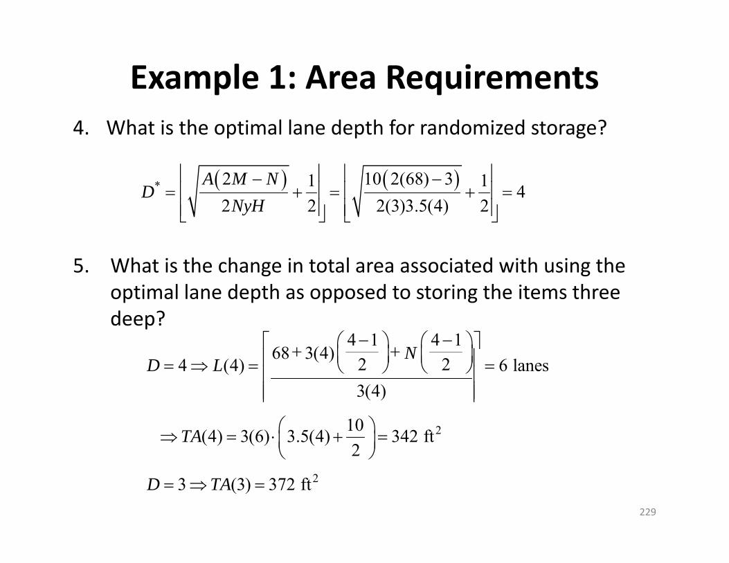
Example 1: Area Requirements4. What is the optimal lane depth for randomized storage?

5. What is the change in total area associated with using the optimal lane depth as opposed to storing the items three deep?

229

* 2 10 2(68) 31 1 42 2 2(3)3.5(4) 2

A M ND

NyH

2

2

4 1 4 168 3(4) 2 24 (4) 6 lanes

3(4)

10(4) 3(6) 3.5(4) 342 ft2

3 (3) 372 ft

ND L

TA

D TA

Example 2: Trailer LoadingHow many identical 48  42  36 in. four‐way containers can be shipped in a full truckload? Each container load:

1. Weighs 600 lb2. Can be stacked up to six high without causing damage from crushing3. Can be rotated on the trucks with respect to their width and depth.

230

Truck Trailer

Cube = 3,332 - 3,968 CFTMax Gross Vehicle Wt = 80,000 lbs = 40 tons

Max Payload Wt = 50,000 lbs = 25 tons

Length: 48' - 53' single trailer, 28' double trailer

Inte

rior H

eigh

t:(8

'6" -

9'2"

= 1

02" -

110"

)

Width:

8'6" = 102"

(8'2" = 98")

Max

Hei

ght:

13

'6" =

162

"

Max of 83 units per TL

X 98/12 = 8.166667 8.166667 ftY 53 53 ftZ 110/12 = 9.166667 9.166667 ftx [48,42]/12 = 4 3.5 fty [42,48]/12 = 3.5 4 ftz 30/12 = 2.5 2.5 ftL floor(X/x) = 2 2D floor(Y/y) = 15 13H min(6,floor(Z/z)) = 3 3

LDH L*D*H = 90 78 unitswt 600 600 lb

unit/TL min(LDH, floor(50000/wt)) = 83 78

Storage and Retrieval Cycle• A storage and retrieval (S/R) cycle is one complete roundtrip from an I/O port to slot(s) and back to the I/O

• Type of cycle depends on load carrying ability:– Carrying one load at‐a‐time (load carried on a pallet):

• Single command• Dual command

– Carrying multiple loads (order picking of small items):

• Multiple command

231

Single‐Command S/R Cycle

store

empty

empty

retrieve

I/Oslot

232

• Single‐command (SC) cycles:– Storage: carry one load to slot for storage and return empty back to I/O port, or

– Retrieval: travel empty to slot to retrieve load and return with it back to I/O port

/2SC SCSC L U L U

d dt t t tv v

Expected time for each SC S/R cycle:

Industrial Trucks: Walk vs. RideWalk (2 mph = 176 fpm) Ride (7 mph = 616 fpm)

Pallet Jack Pallet Truck

Walkie Stacker Sit‐down Counterbalanced Lift Truck

233

Dual‐Command S/R Cycle

234

• Dual‐command (DC):• Combine storage with a retrieval:– store load in slot 1, travel empty to slot 2 to retrieve load

• Can reduce travel distance by a third, on average

• Also termed task “interleaving”

/2 2 4DC DCDC L U L U

d dt t t tv v

Expected time for each SC S/R cycle:

Multi‐Command S/R Cycle

empty

retrieve

I/O

235

• Multi‐command: multiple loads can be carried at the same time

• Used in case and piece order picking

• Picker routed to slots– Simple VRP procedures can be used

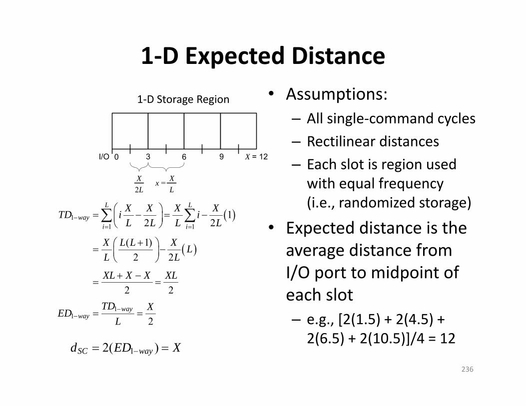
1‐D Expected Distance

11 1

11

12 2

( 1)2 2

2 2

2

L L

wayi i

wayway

X X X XTD i iL L L L

X L L X LL L

XL X X XL

TD XEDL

236

• Assumptions:– All single‐command cycles– Rectilinear distances– Each slot is region used with equal frequency (i.e., randomized storage)

• Expected distance is the average distance from I/O port to midpoint of each slot– e.g., [2(1.5) + 2(4.5) + 2(6.5) + 2(10.5)]/4 = 12

I/O 3 6 9 X = 12

X XL

0

2Lx =

1‐D Storage Region

12( )SC wayd ED X

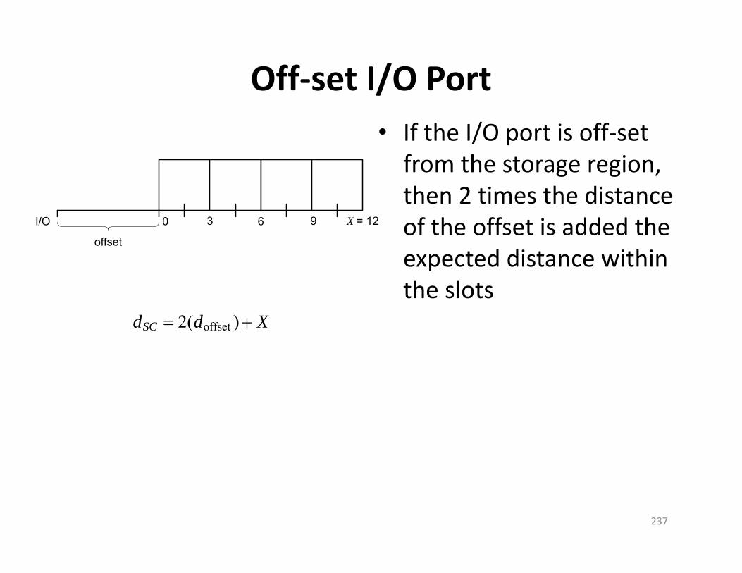
Off‐set I/O Port

I/O 3 6 9 X = 120

offset

237

• If the I/O port is off‐set from the storage region, then 2 times the distance of the offset is added the expected distance within the slots

offset2( )SCd d X

2‐D Expected Distances• Since dimensions X and Y are independent of each other for 

rectilinear distances, the expected distance for a 2‐D rectangular region with the I/O port in a corner is just the sum of the distance in X and in Y:

• For a triangular region with the I/O port in the corner:

238

rectSCd X Y

1

1-way1 1

2

1-way1-way

2 2

2 3 16

2 2 , as( 1) 3 3 32

2 21 12 23 33 3

L L i

i j

triSC

X X X XTD i jL L L L

X L L

TD XED X X LL L L

d X X Y X Y

I/O XXxL

Y

YyD

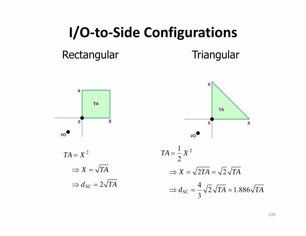
I/O‐to‐Side ConfigurationsRectangular Triangular

239

212

2 2

4 2 1.8863SC

TA X

X TA TA

d TA TA

2

2SC

TA X

X TA

d TA

TA

I/O

0 X

X

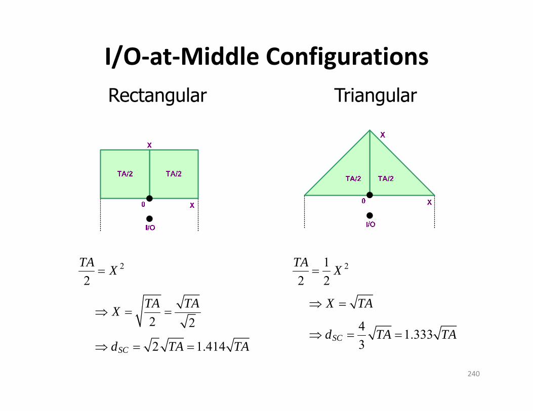
I/O‐at‐Middle ConfigurationsRectangular Triangular

240

212 2

4 1.3333SC

TA X

X TA

d TA TA

2

2

2 2

2 1.414SC

TA X

TA TAX

d TA TA

Example 3: Handling RequirementsPallet loads will be unloaded at the receiving dock of a warehouse and placed on the floor. From there, they will be transported 500 feet using a dedicated pallet truck to the in‐floor induction conveyor of an AS/RS. Given

a. It takes 30 sec to load each pallet at the dockb. 30 sec to unload it at the induction conveyorc. There will be 80,000 loads per year on averaged. Operator rides on the truck (because a pallet truck)e. Facility will operate 50 weeks per year, 40 hours per week

241

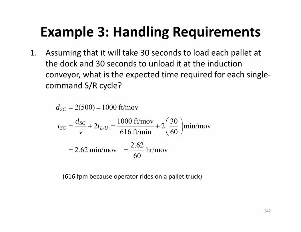
Example 3: Handling Requirements1. Assuming that it will take 30 seconds to load each pallet at 

the dock and 30 seconds to unload it at the induction conveyor, what is the expected time required for each single‐command S/R cycle?

242

/

2(500) 1000 ft/mov

1000 ft/mov 302 2 min/mov616 ft/min 60

2.622.62 min/mov hr/mov60

SC

SCSC L U

d

dt tv

(616 fpm because operator rides on a pallet truck)

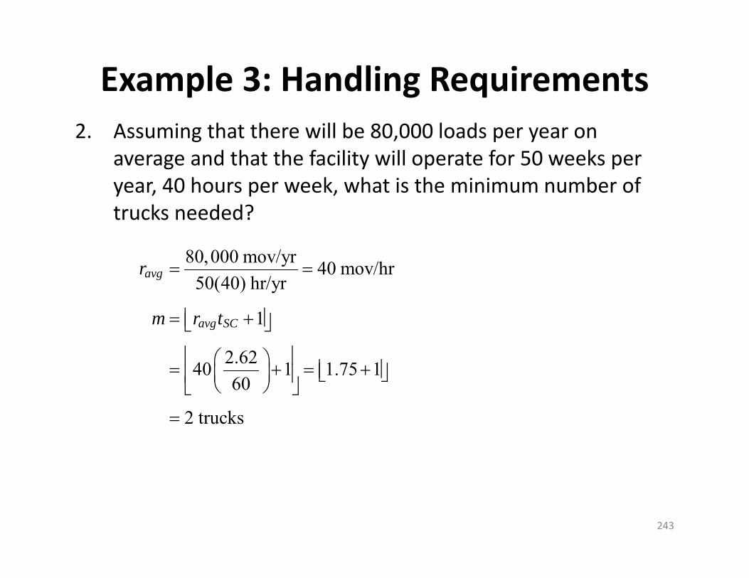
Example 3: Handling Requirements2. Assuming that there will be 80,000 loads per year on 

average and that the facility will operate for 50 weeks per year, 40 hours per week, what is the minimum number of trucks needed?

243

80,000 mov/yr 40 mov/hr50(40) hr/yr

1

2.6240 1 1.75 160

2 trucks

avg

avg SC

r

m r t

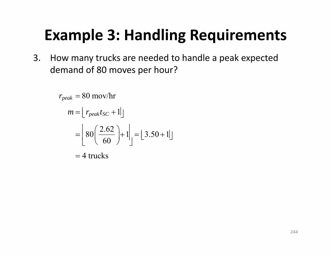
Example 3: Handling Requirements3. How many trucks are needed to handle a peak expected 

demand of 80 moves per hour?

244

80 mov/hr

1

2.6280 1 3.50 160

4 trucks

peak

peak SC

r

m r t

Example 3: Handling Requirements4. If, instead of unloading at the conveyor, the 3‐foot‐wide 

loads are placed side‐by‐side in a staging area along one side of 90‐foot aisle that begins 30 feet from the dock, what is the expected time required for each single‐command S/R cycle?

245

offset

/

2( ) 2(30) 90 150 ft

150 ft/mov 302 2 min/mov616 ft/min 60

1.241.24 min/mov hr/mov60

SC

SCSC L U

d d X

dt tv

Estimating Handling Costs• Warehouse design involves the trade‐off between building 

and handling cost.• Maximizing the cube utilization of a storage region will help 

minimize building costs.• Handling costs can be estimated by determining:

1. Expected time required for each move based on an average of the time required to reach each slot in the region.

2. Number of vehicles needed to handle a target peak demand for moves, e.g., moves per hour.

3. Operating costs per hour of vehicle operation, e.g., labor, fuel (assuming the operators can perform other productive tasks when not operating a truck)

4. Annual operating costs based on annual demand for moves.5. Total handling costs as the sum of the annual capital recovery costs 

for the vehicles and the annual operating costs.

246

Example 4: Estimating Handing Cost

247

I/O

TA = 20,000

/

peak

year

Expected Distance: 2 2 20,000 200 ft

Expected Time: 2

200 ft 2(0.5 min) 2 min per move200 fpm

Peak Demand: 75 moves per hour

Annual Demand: 100,000 moves per year

Number of T

SC

SCSC L U

d TA

dt tv

r

r

peak

hand truck year labor

rucks: 1 3.5 3 trucks60

Handling Cost:60

23($2,500 / tr-yr) 100,000 ($10 / hr)60

$7,500 $33,333 $40,833 per year

SC

SC

tm r

tTC mK r C

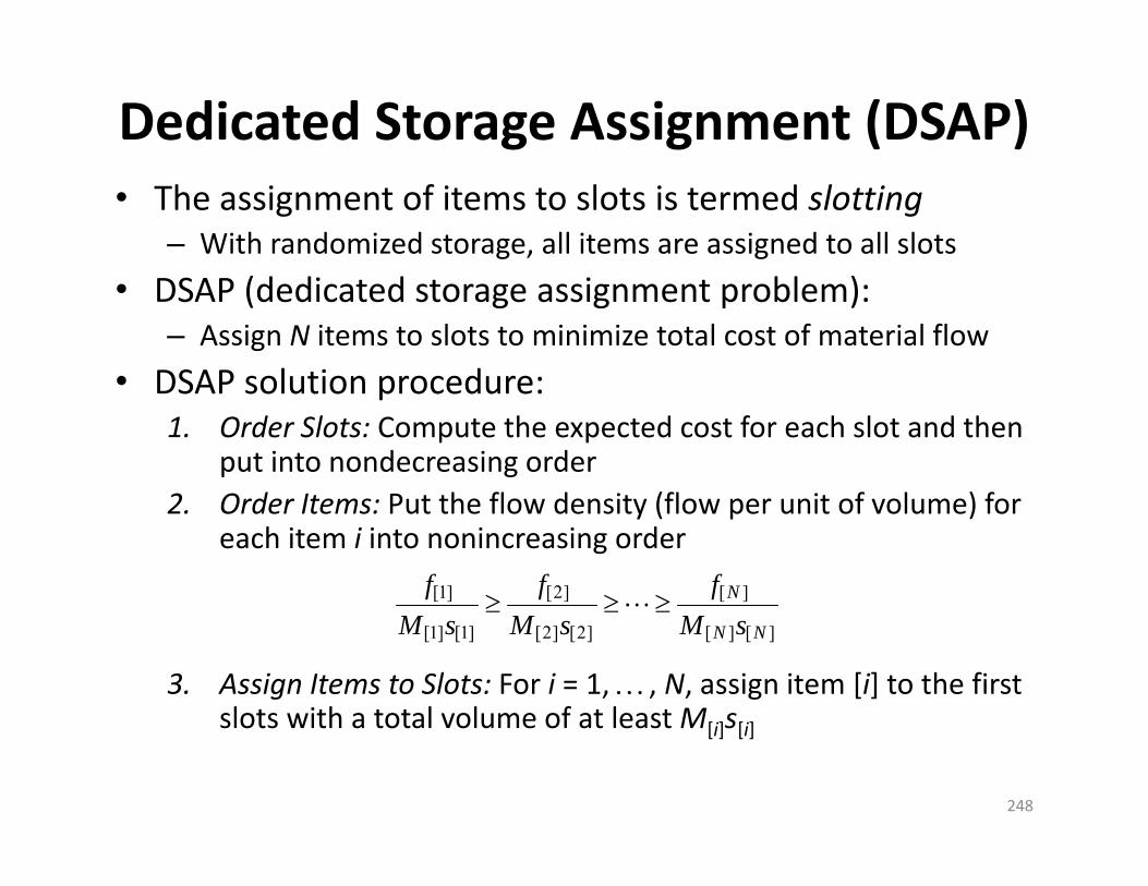
Dedicated Storage Assignment (DSAP)• The assignment of items to slots is termed slotting

– With randomized storage, all items are assigned to all slots• DSAP (dedicated storage assignment problem):

– Assign N items to slots to minimize total cost of material flow• DSAP solution procedure:

1. Order Slots: Compute the expected cost for each slot and then put into nondecreasing order

2. Order Items: Put the flow density (flow per unit of volume) for each item i into nonincreasing order

3. Assign Items to Slots: For i = 1, , N, assign item [i] to the first slots with a total volume of at least M[i]s[i]

248

[1] [2] [ ]

[1] [1] [2] [2] [ ] [ ]

N

N N

f f fM s M s M s

1‐D Slotting Example

249

Flow Density

1-D Slot Assignments

Expected Distance Flow

Total Distance

21 7.003 C C C

I/O30

2(0) + 3 = 3 21 = 63

24 6.004

A A A AI/O

-3 0 4 2(3) + 4 = 10 24 = 240

7 1.405

B BI/O

B B B

-7 50 2(7) + 5 = 19 7 = 133

C C C A A A A B B

I/OB B B

0 7 123 436

A B C Max units M 4 5 3 Space/unit s 1 1 1 Flow f 24 7 21 Flow Density f/(M x s) 6.00 1.40 7.00

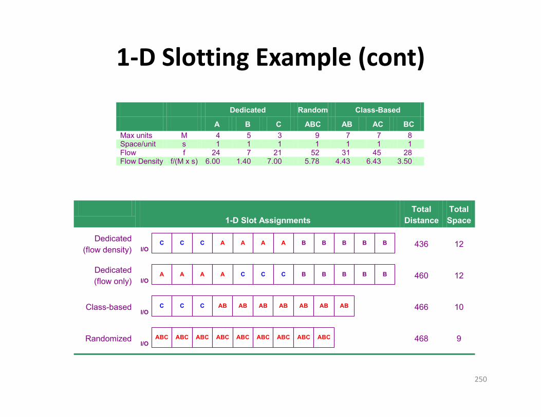
1‐D Slotting Example (cont)

Dedicated Random Class-Based

A B C ABC AB AC BC Max units M 4 5 3 9 7 7 8 Space/unit s 1 1 1 1 1 1 1 Flow f 24 7 21 52 31 45 28 Flow Density f/(M x s) 6.00 1.40 7.00 5.78 4.43 6.43 3.50

250

1-D Slot Assignments

Total Distance

Total Space

Dedicated (flow density)

C C C A A A A B BI/O

B B B

436 12

Dedicated (flow only)

A A A A C C C B BI/O

B B B

460 12

Class-based C C C AB AB AB AB AB ABI/O

AB

466 10

Randomized ABC ABC ABC ABC ABC ABC ABC ABC ABCI/O

468 9

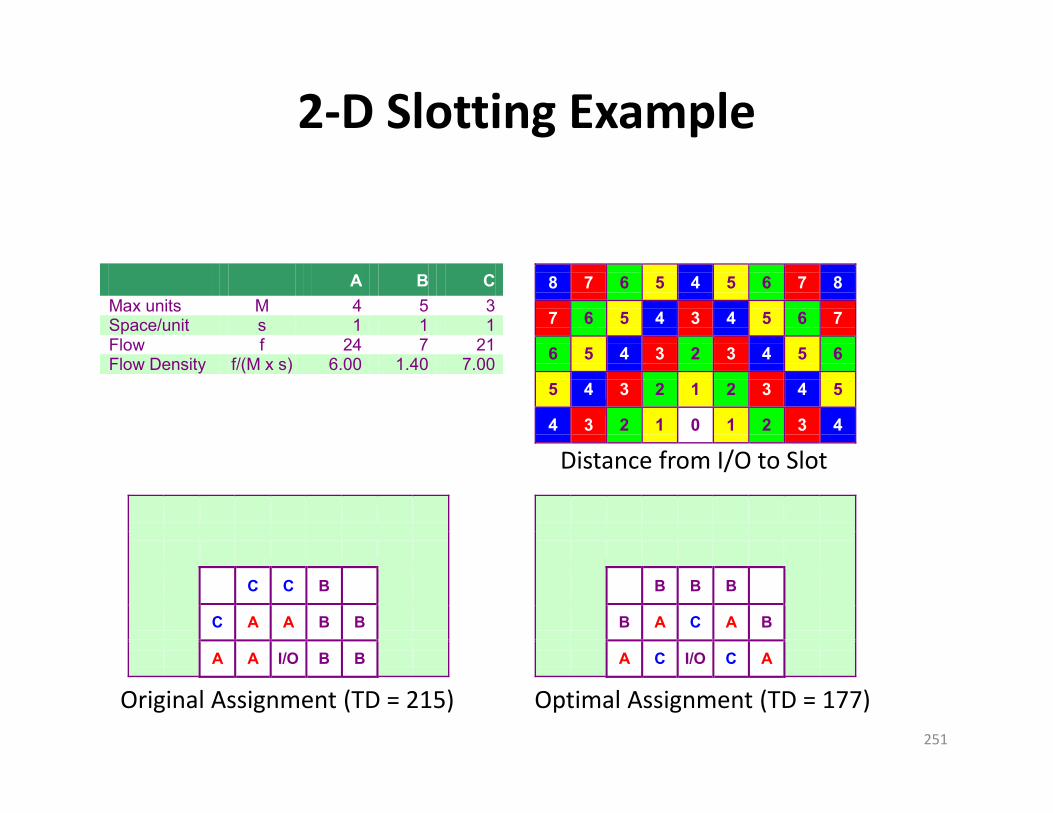
2‐D Slotting Example

A B C Max units M 4 5 3 Space/unit s 1 1 1 Flow f 24 7 21 Flow Density f/(M x s) 6.00 1.40 7.00

251

8 7 6 5 4 5 6 7 8

7 6 5 4 3 4 5 6 7

6 5 4 3 2 3 4 5 6

5 4 3 2 1 2 3 4 5

4 3 2 1 0 1 2 3 4

Original Assignment (TD = 215) Optimal Assignment (TD = 177)

C C B

C A A B B

A A I/O B B

B B B

B A C A B

A C I/O C A

Distance from I/O to Slot

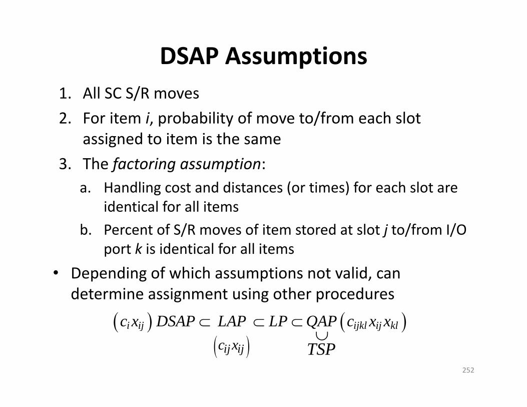
DSAP Assumptions1. All SC S/R moves2. For item i, probability of move to/from each slot 

assigned to item is the same3. The factoring assumption:

a. Handling cost and distances (or times) for each slot are identical for all items

b. Percent of S/R moves of item stored at slot j to/from I/O port k is identical for all items

• Depending of which assumptions not valid, can determine assignment using other procedures 

252

i ij ijkl ij kl

ij ijc xc x DSAP LAP LP QAP c x x

TSP

Example 5: 1‐D DSAP• What is the change in the minimum expected total distance traveled if dedicated, as compared to randomized, block stacking is used, wherea. Slots located on one side of 10‐foot‐wide down aisleb. All single‐command S/R operationsc. Each lane is three‐deep, four‐highd. 40  36 in. two‐way pallet used for all loadse. Max inventory levels of SKUs A, B, C are 94, 64, and 50f. Inventory levels are uncorrelated and retrievals occur at a 

constant rateg. Throughput requirements of A, B, C  are 160, 140, 130h. Single I/O port is located at the end of the aisle

253

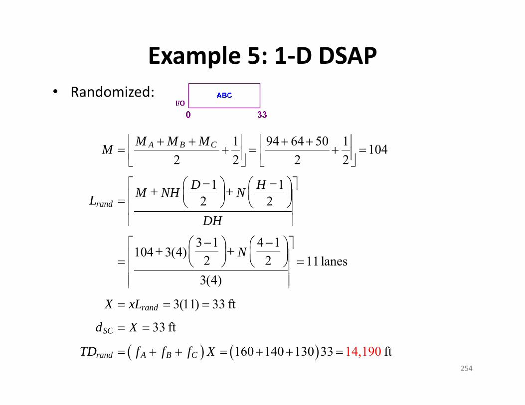
Example 5: 1‐D DSAP

254

• Randomized:

14

1 94 64 50 1 1042 2 2 2

1 12 2

3 1 4 1104 3(4) 2 2 11 lanes

3(4)

3(11) 33 ft

33 ft

160 140 130 33

A B C

rand

rand

SC

rand A B C

M M MM

D HM NH NLDH

N

X xL

d X

TD f f f X

,190 ft

Example 5: 1‐D DSAP

255

• Dedicated:

160 140 1301.7, 2.19, 2.694 64 50

94 64 508, 6, 53(4) 3(4) 3(4)

3(5) 15, 3(6) 18, 3(8) 24

3(5) 15 ft

A B C

A B C

A B CA B C

C C B B A A

CSC C

S

f f f C B AM M M

M M ML L LDH DH DH

X xL X xL X xL

d X

d

2( ) 2(15) 18 48 ft

2( ) 2(15 18) 24 90 ft

160(90) 140(48) 130 23,01 0( 75) ft

BC C B

ASC C B A

A B Cded A SC B SC C SC

X X

d X X X

TD f d f d f d

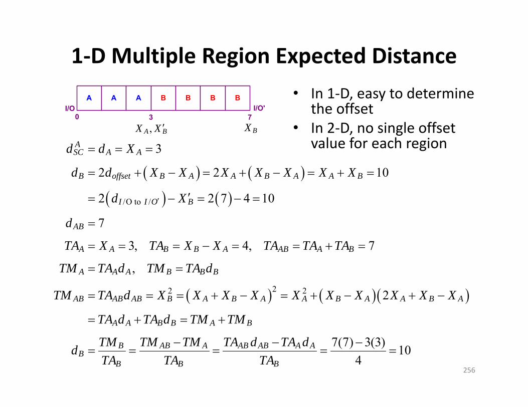
1‐D Multiple Region Expected Distance• In 1‐D, easy to determine 

the offset• In 2‐D, no single offset 

value for each region

256

/O to /

22 2

3

2 2 10

2 2 7 4 10

7

3, 4, 7

,

2

ASC A A

B offset B A A B A A B

I I O B

AB

A A B B A AB A B

A A A B B B

AB AB AB B A B A A B A A B A

A A B B A B

B

d d X

d d X X X X X X X

d X

d

TA X TA X X TA TA TA

TM TA d TM TA d

TM TA d X X X X X X X X X X

TA d TA d TM TM

Td

7(7) 3(3) 10

4B AB A AB AB A A

B B B

M TM TM TA d TA dTA TA TA

A A A B B B BI/O

0 3 7I/Oʹ

BX,A BX X

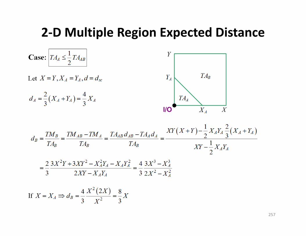
2‐D Multiple Region Expected Distance

257

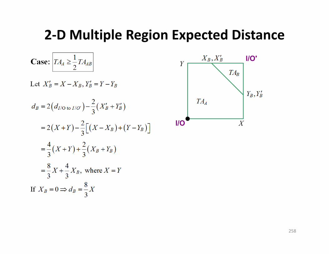
2‐D Multiple Region Expected Distance

258

2‐D Multiple Region Expected Distance• If more than two regions

– For regions below diagonal (D), start with region closest to I/O– For regions above diagonal (A+C), start with regions closest to 

I/O’ (C)– For region in the middle (B), solve using whole area less other 

regions

259

AX CX

DX

Warehouse OperationsPu

taw

ay

Order Picking

Putawa

y

260

Warehouse Management System• WMS interfaces with a corporation’s enterprise resource 

planning (ERP) and the control software of each MHS

261• Advance shipping notice (ASN) is a standard format used for communications

ItemOn-HandBalance

In-TransitQty. Locations

A 2 1 11,21B 4 0 12,22

Inventory Master File

Location ItemOn-HandBalance

In-TransitQty.

11 A 1 012 B 3 021 A 1 122 B 1 0

Location Master File

A

B B B

A

B

11

12

21

22

A

Logistics‐related Codes Commodity Code Item Code Unit Code

Level Category Class Instance Description Grouping of

similar objects Grouping of identical

objects Unique

physical object Function Product

classification Inventory control Object

tracking Names — Item number, Part number,

SKU, SKU + Lot number Serial number, License plate

Codes UNSPSC, GPC

GTIN, UPC, ISBN, NDC

EPC, SSCC

262

UNSPSC: United Nations Standard Products and Services CodeGPC: Global Product CatalogueGTIN: Global Trade Item Number (includes UPC, ISBN, and NDC)UPC: Universal Product CodeISBN: International Standard Book NumberingNDC: National Drug CodeEPC: Electronic Product Code (globally unique serial number for physical objects

identified using RFID tags)SSCC: Serial Shipping Container Code (globally unique serial number for 

identifying movable units (carton, pallet, trailer, etc.))

Identifying Storage Locations

263

0103

0911

0507

A

B

C

D

E

Bay (X)

Tier

(Z)

Aisle (Y)AAB

AAC

AAA

Cross AisleDown Aisle

Wall

Compartment

12A

B

Position

Location: 1 -AAC - 09 - D - 1 - B

Buildin

gAisle Bay Tier Pos

ition

Compa

rtmen

t

Receiving

264

• Basic steps:1. Unload material from trailer.2. Identify supplier with ASN, and associate material with each 

moveable unit listed in ASN.3. Assign inventory attributes to movable unit from item 

master file, possibly including repackaging and assigning new serial number.

4. Inspect material, possibly including holding some or all of the material for testing, and report any variances.

5. Stage units in preparation for putaway.6. Update item balance in inventory master and assign units to 

a receiving area in location master.7. Create receipt confirmation record.8. Add units to putaway queue

ReserveStorageReceive Putaway Replenish Forward

PickOrderPick

Sort &Pack Ship

Putaway

265

• A putaway algorithm is used in WMS to search for and validate locations where each movable unit in the putaway queue can be stored

• Inventory and location attributes used in the algorithm:– Environment (refrigerated, caged area, etc.)– Container type (pallet, case, or piece)– Product processing type (e.g., floor, conveyable, nonconveyable)

– Velocity (assign to A, B, C based on throughput of item)– Preferred putaway zone (item should be stored in same zone as related items in order to improve picking efficiency)

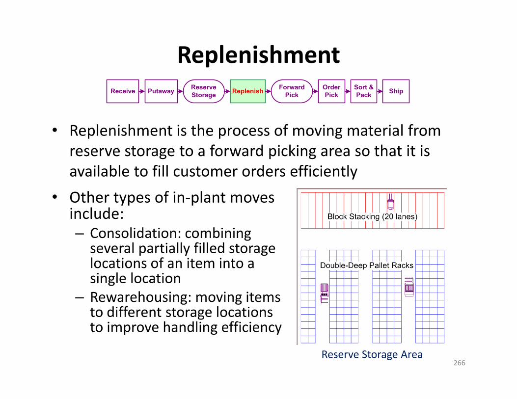
Replenishment

266

• Other types of in‐plant moves include:– Consolidation: combining several partially filled storage locations of an item into a single location

– Rewarehousing: moving items to different storage locations to improve handling efficiency

ReserveStorageReceive Putaway Replenish Forward

PickOrderPick

Sort &Pack Ship

• Replenishment is the process of moving material from reserve storage to a forward picking area so that it is available to fill customer orders efficiently

Reserve Storage Area

Order Picking

267

• Order picking is at the intersection of warehousing and order processing

WH Operating Costs

ReserveStorageReceive Putaway Replenish Forward

PickOrderPick

Sort &Pack Ship

Receiving10%

Storage15%

Order Picking55%

Shipping20%

Information P

rocessing

Material Handling

Putaway Storage Order Picking Shipping

Order Entry

OrderTransmittal

Order StatusReporting

Order Processing

War

ehou

sing

Receiving

OrderPreparation

Order Picking

268

Levels of Order Picking

ReserveStorageReceive Putaway Replenish Forward

PickOrderPick

Sort &Pack Ship

Case Picking

Pallet Picking

Piece Picking

Pallet and Case Picking Area

Forward Piece Picking Area

Order Picking

269

ReserveStorageReceive Putaway Replenish Forward

PickOrderPick

Sort &Pack Ship

Voice‐Directed Piece and Case Picking

Pick 24 Pack 14

Pack 10

Carton Flow Rack Picking Cart

Confirm Button

Increment/Decrement

Buttons

Count Display

Pick‐to‐Light Piece Picking

Order Picking

270

ReserveStorageReceive Putaway Replenish Forward

PickOrderPick

Sort &Pack Ship

Methods of Order Picking

DA B C E F G H

1

2

3

4

5

6

7 A3

Picker 1

Zone 1

Picker 2

Zone 2

C7D5

G1

B4

F2

E8

Method

Pickers per

Order

Orders per

Picker Discrete Single Single Zone Multiple Single Batch Single Multiple Zone-Batch Multiple Multiple

Discrete

Batch

Zone

Zone‐Batch

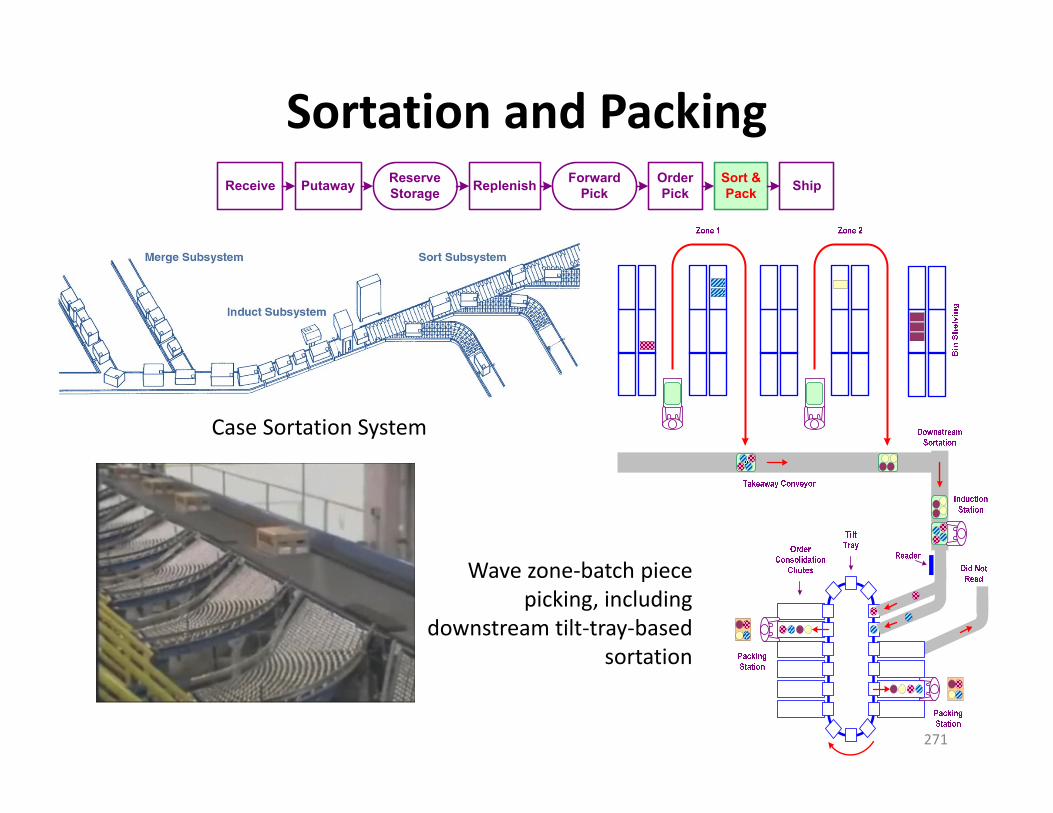
Sortation and Packing

271

Wave zone‐batch piece picking, including 

downstream tilt‐tray‐based sortation

ReserveStorageReceive Putaway Replenish Forward

PickOrderPick

Sort &Pack Ship

Case Sortation System

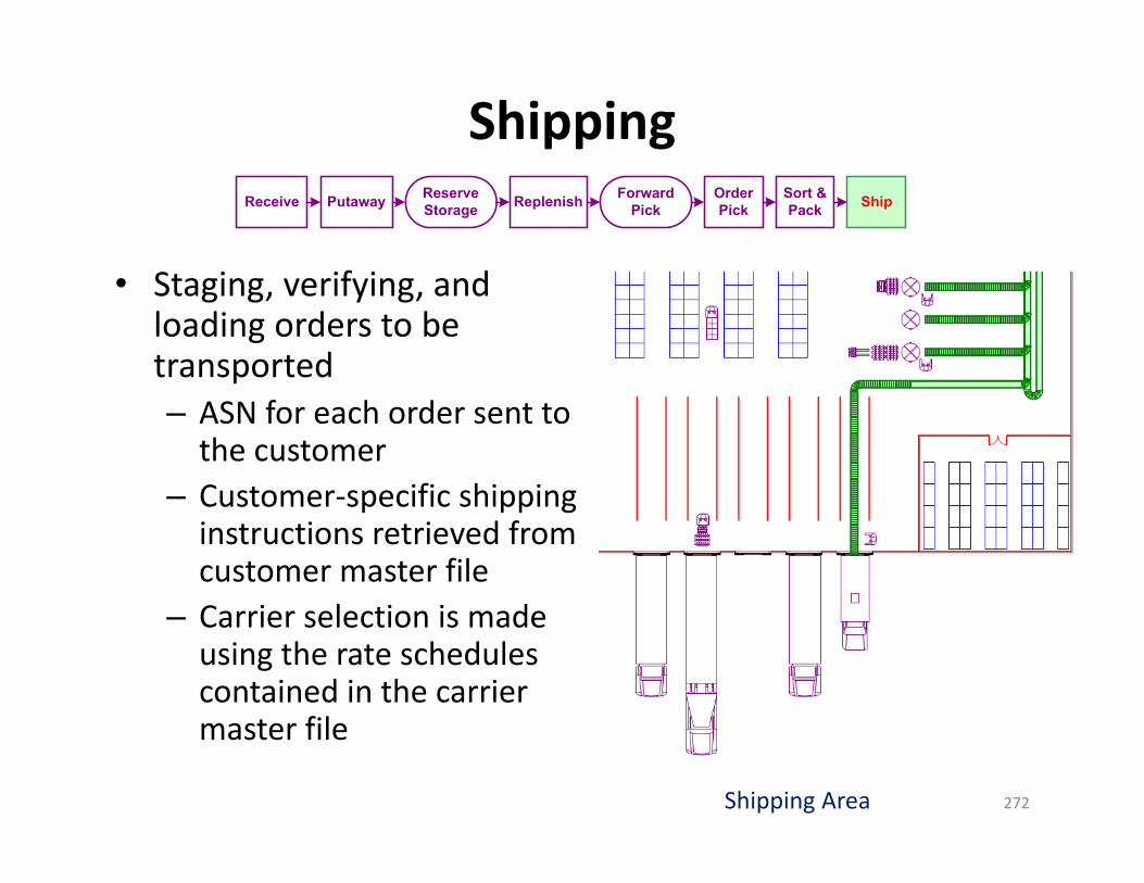
Shipping

272

• Staging, verifying, and loading orders to be transported– ASN for each order sent to the customer

– Customer‐specific shipping instructions retrieved from customer master file

– Carrier selection is made using the rate schedules contained in the carrier master file

Shipping Area

ReserveStorageReceive Putaway Replenish Forward

PickOrderPick

Sort &Pack Ship

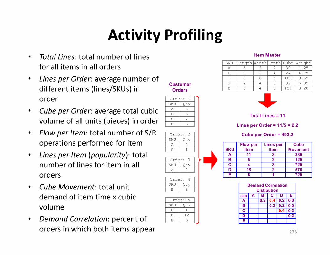
Activity Profiling• Total Lines: total number of lines 

for all items in all orders• Lines per Order: average number of 

different items (lines/SKUs) in order

• Cube per Order: average total cubic volume of all units (pieces) in order

• Flow per Item: total number of S/R operations performed for item

• Lines per Item (popularity): total number of lines for item in all orders

• Cube Movement: total unit demand of item time x cubic volume

• Demand Correlation: percent of orders in which both items appear 273

SKU B D EA 0.2 0.2 0.0

C 0.4 0.2

Demand Correlation Distibution

D 0.2E

A

B 0.2 0.0

C0.40.2

SKUCube

MovementA 330

C 720D 576E 720

Lines per Item

3

321

B 2 120

Flow per Item1154

186

Total Lines = 11

Lines per Order = 11/5 = 2.2

Cube per Order = 493.2

SKU Width Cube WeightA 3 30 1.25

C 6 180 9.65D 4 32 6.35E 4 120 8.20

Length5

846

B 3 2 24 4.75

Depth24535

Item Master

SKUAB

Order: 1

CD

Qty5326

SKUCD

Order: 5

E

Qty1126

SKUA

Order: 3Qty2

SKUA

Order: 2

C

Qty41

SKUB

Order: 4Qty2

Customer Orders

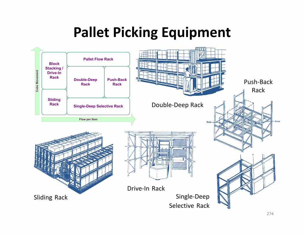
Pallet Picking Equipment

274

Single-Deep Selective Rack

Double-DeepRack

Push-BackRack

Sliding Rack

Block Stacking / Drive-In

Rack

Pallet Flow Rack

Flow per Item

Cub

e M

ovem

ent

Drive‐In RackSliding Rack Single‐Deep

Selective Rack

Double‐Deep Rack

Push‐BackRack

Case Picking

275

FlowDelivery

Lanes

Single-DeepSelective Rack

Pallet FlowRack

Lines per Item

Cube

Mov

emen

t

CaseDispensers

Push BackRack

Manual Automated Case PickingEquipment

Unitizing and

Shipping

Sort

atio

n C

onve

yor

InductInduct

Single-DeepSelective

Racks

Zone‐Batch Pick to Pallet

Floor‐ vs. Multi‐levelPick to Pallet

Case Picking

Rep

leni

sh

Res

erve

Sto

rage

Forw

ard

Pick

St

orag

e

Case Picking

Forw

ard

Pick

Sto

rage

Case Picking

Case Picking

Case Picking

Floor-level Pick Multi-level Pick

Piece Picking Equipment

276

Bin Shelving HorizontalCarousel

StorageDrawers

Carton Flow Rack

Lines per Item

Cube

Mov

emen

t

A-FrameVertical Lift

Module

A‐FrameDispenser

Carousel

Carton Flow Rack

Drawers/Bins

Vertical Lift Module

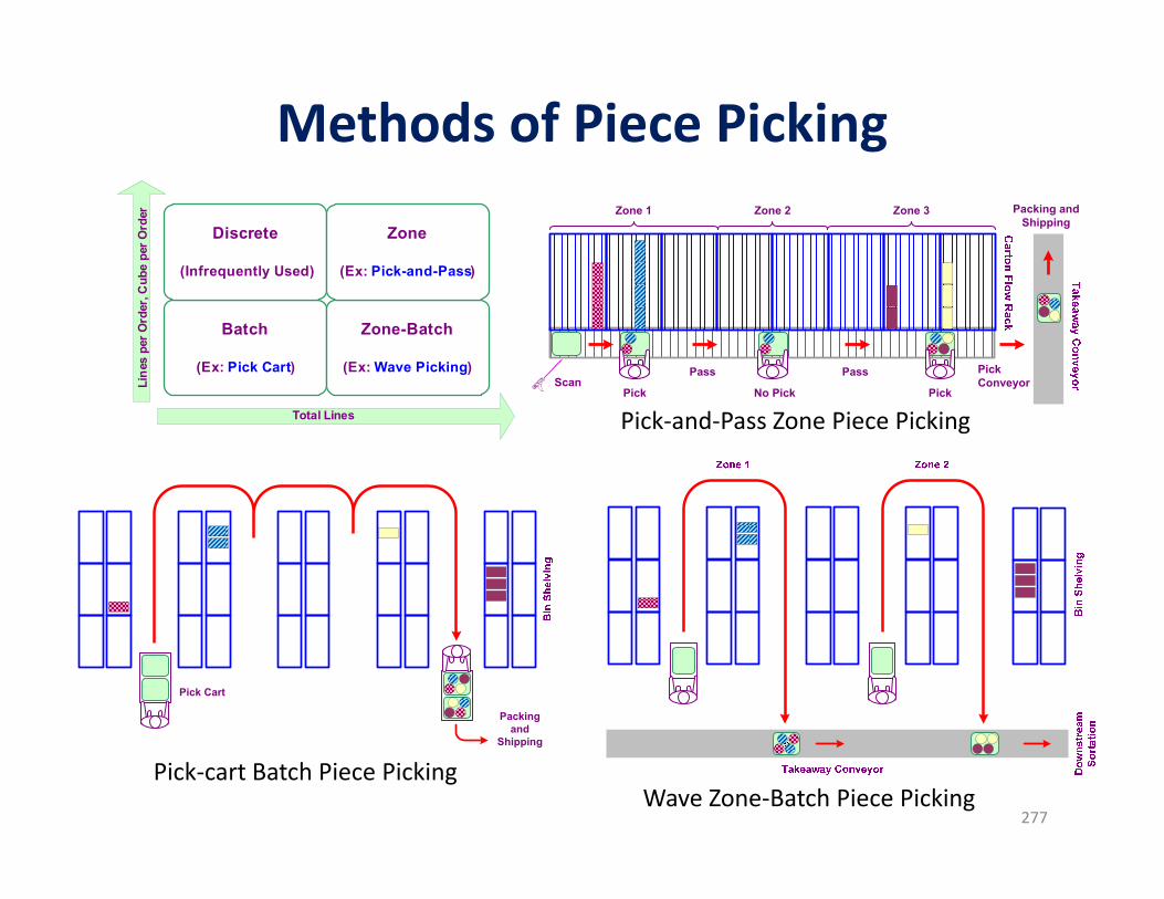
Methods of Piece Picking

277

Batch

(Ex: Pick Cart)

Zone-Batch

(Ex: Wave Picking)

Discrete

(Infrequently Used)

Zone

(Ex: Pick-and-Pass)

Line

s pe

r Ord

er, C

ube

per O

rder

Total Lines

Packing and

Shipping

Pick Cart

Packing and Shipping

Zone 1 Zone 2 Zone 3

Pick Pick

PassPass Pick Conveyor

No PickScan

Pick‐cart Batch Piece PickingWave Zone‐Batch Piece Picking

Pick‐and‐Pass Zone Piece Picking

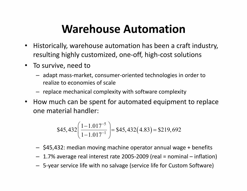
Warehouse Automation• Historically, warehouse automation has been a craft industry, 

resulting highly customized, one‐off, high‐cost solutions• To survive, need to

– adapt mass‐market, consumer‐oriented technologies in order to realize to economies of scale

– replace mechanical complexity with software complexity

• How much can be spent for automated equipment to replace one material handler:

– $45,432: median moving machine operator annual wage + benefits– 1.7% average real interest rate 2005‐2009 (real = nominal – inflation)– 5‐year service life with no salvage (service life for Custom Software)

5

11 1.017$45,432 $45, 432 4.83 $219,6921 1.017

KIVA Mobile‐Robotic Fulfillment System

• Goods‐to‐man order picking and fulfillment system• Multi‐agent‐based control

– Developed by Peter Wurman, former NCSU CSC professor

• Kiva now called Amazon Robotics– purchased by Amazon in 2012 for $775 million

Study Guide for Final Exam10. Second material: infer all flows from given data

28012 25 5

20

0

0

16 17 17

0 20 30

0 17 33

16 13 0

0 3 0

8 0 28

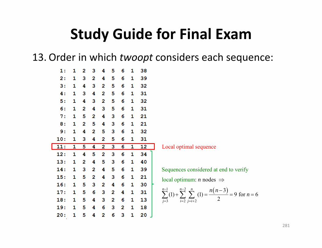
Study Guide for Final Exam13. Order in which twoopt considers each sequence:

281

1 2

3 2 2

Sequences considered at end to verify

local : nodes

3(1) (1) 9 for

o ti u

6

p m

2

mn n n

j i j i

n

n nn

Local optimal sequence

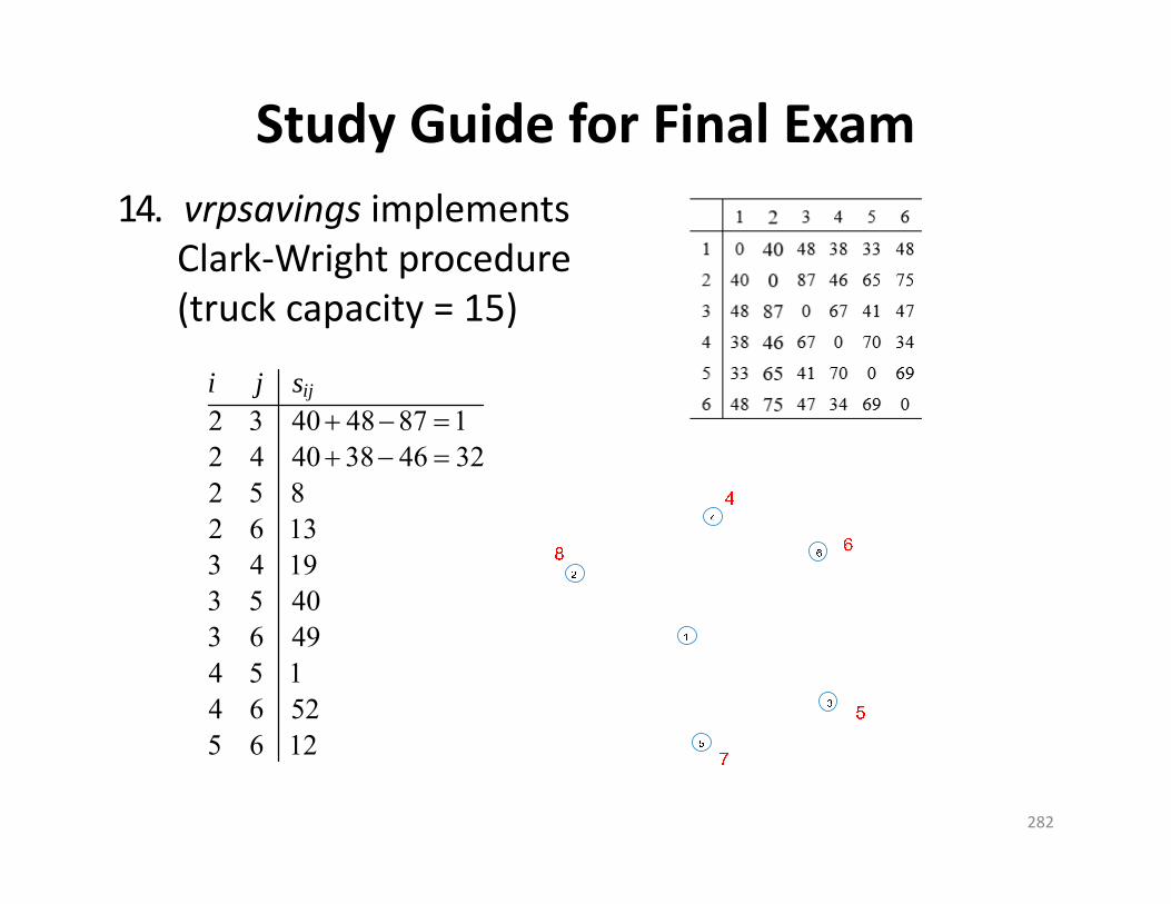
Study Guide for Final Exam14. vrpsavings implements 

Clark‐Wright procedure(truck capacity = 15)

282

2 3 40 48 87 12 4 40 38 46 322 5 82 6 133 4 193 5 403 6 494 5 14 6 525 6 12

iji j s

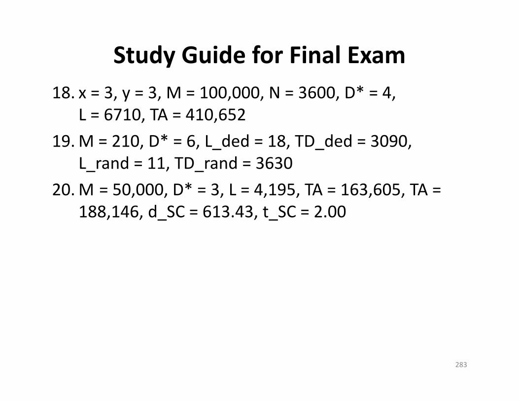
Study Guide for Final Exam18. x = 3, y = 3, M = 100,000, N = 3600, D* = 4, 

L = 6710, TA = 410,65219.M = 210, D* = 6, L_ded = 18, TD_ded = 3090, 

L_rand = 11, TD_rand = 363020.M = 50,000, D* = 3, L = 4,195, TA = 163,605, TA = 

188,146, d_SC = 613.43, t_SC = 2.00

283

Study Guide for Final Exam22.

284

2 31.62

2 / 2 24.49

17.32

24.49

D D

C C C C

A A C A A

X TA

X TA

X TA X X X

X TA TA X X X

AX CX

DX