iscwsa recap & introduction - | iadd
TRANSCRIPT

111
ISCWSA
Recap &
Introduction

What is ISCWSA
2
The Industry Steering Committee on Wellbore Survey Accuracy
SPE WPTS – Wellbore Positioning Technical Section
Mission Statement
"The primary aim of this group is to produce and maintain standards for the industry relating
to wellbore survey accuracy.“
"To set standards for terminology and accuracy specifications. Establish a standard
framework for modelling and validation of tool performance. Raise awareness &
understanding of wellbore survey accuracy issues across the industry."

Who Can Join
3
Anyone is free to attend any ISCWSA meetings.
This includes but is not limited to
• Well Planners
• Coordinators
• Field Hands
• Software Developers
• Tool Manufacturers
• Drilling Engineers
• Technology Companies
• People with General Interest in Survey Accuracy
• All
Meetings
4
Meetings are held twice a year.
One meeting has to be held in conjunction with SPE ATCE
Next Meeting TBD
Previous Meeting
Last Week Glasgow, Scotland

Subcommittee Meetings
5
Meetings are held the normally the day before.
Sub committee meeting are open to all.
• Well Intercept
• Error Model Management
• Collision Avoidance
• Operator’s Wellbore Survey Group
• Education
Attendees are those who can contribute to that specific group. (Voluntary Work)

Directors and Chairs
6
Chair Person: Son Pham, ConocoPhillips
Program Chair: Jonathan Lightfoot, Occidental Oil and Gas Corporation
Secretary Chad Hanak, SuperiorQC
Treasurer: Robert Wylie, NOV
Webmaster: Phil Harbidge, Schlumberger
Director at large: Carol Mann, Dynamic Graphics Inc.
Director at large: Andy McGregor, Tech21
Well Intercept Roger Goobie, BP
Error Model Management Andy McGregor, Tech21
Collision Avoidance Steve Sawaryn
Operator’s Wellbore Survey Group Pete Clark, Chevron
Education Steve Mullin
Recap
Keynote Address
6 Technical Presentations
Guest Speaker
5 Sub-Committee Updates
7
888
TECHNICAL PRESENTATIONSSwarm Satellite Data to Improve Global Geomagnetic Reference
Modelling
Ciarán Beggan, British Geological Survey
Technical Presentations
Swarm Satellite Data to Improve Global Geomagnetic Reference Modelling
– Ciarán Beggan, British Geological Survey
Earth’s Magnetic Environment
ESA Swarm Mission
Secular Variation: Jerks, IGRF, and Model Updates
Modelling Uncertainties
Summary
9
10
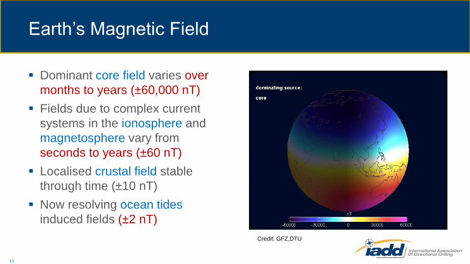
Earth’s Magnetic Field
Dominant core field varies over
months to years (±60,000 nT)
Fields due to complex current
systems in the ionosphere and
magnetosphere vary from
seconds to years (±60 nT)
Localised crustal field stable
through time (±10 nT)
Now resolving ocean tides
induced fields (±2 nT)
Credit: GFZ,DTU

ESA Swarm Mission
Novel 3-satellite constellation
– 2 lower satellites
– 1 in higher orbit
Gradient data calculated as difference between two nearby measurements
15-50 second separation along track
Sensitive to local, small scale features
Uses ground observatory data

12
Secular Variation
Flow of liquid iron core generates
secular variation at surface
Non-linear and constantly
changing (‘jerks’)
Current research to improve
understanding

Jerks, IGRF and Importance of Model Updates
13
Due to 2014 jerk, IGRF-12 prediction is 15.7 nT RMS different from recent core field model 2016
IGRF-12
Prediction
s
Summary
Annually updated models necessary to counter large and
unpredictable rapid changes from Earth’s core
Uncertainties are lowering but care needed not to
misunderstand what global models can do
Swarm is promptly delivering a large quantity of highly
accurate measurements
Swarm gradient data offers unique global resolution of
small scale field, especially as orbit lowers
14

151515
TECHNICAL PRESENTATIONSNew Instrument Performance Models for Combined Wellbore
Surveys Facilitate Optimal Use of Survey Information
(SPE – 178826 – MS)
Jon Bang, Gyrodata

New Instrument Performance Models for Combined
Wellbore Surveys Facilitate Optimal Use of Survey
Information (SPE – 178826 – MS)
– Jon Bang, Gyrodata
Introduction/Challenge
Solution
Results
Conclusions
16
Technical Presentations
Benefits of Multiple Surveys
Mutual quality check and validation
Weighted average gives optimal position estimate
Weighted average gives minimum position uncertainty
Two Assumptions
– The surveys must have passed standard quality tests
• no gross errors
– The surveys must all be interpolated to common MD’s
17

Error Analysis Procedure
18

19
Case 1: Incl = 0-30°, N-S

Case 3: Near Horizontal, E-W
20

CONCLUSIONS: AVERAGING METHOD
Individual surveys must pass QC routines: no gross errors
Algorithm– D, I, A weighting factors + adjustment factors
– Analytic, no iteration, suited for automation
Results– Close to true average, conservative
– Any tools, any uncertainties
– Any wellbore profile; best accuracy in tangential sections
– Any number of surveys
Possible challenges– Validation of method for different well profiles
21
CONCLUSIONS: BENEFITS OF AVERAGING
One survey data set per wellbore
Optimal wellbore positions + improved accuracy
Optimize survey programs
Improved reliability of anti-collision calculations
May turn unfeasible projects into achievable ones
– Small drilling targets
– Long extended reach wells
– Highly congested fields
22

232323
TECHNICAL PRESENTATIONSMagnetic Mud
Giorgio Pattarini, University of Stavanger

24
Magnetic Drilling Mud
When the mud is contaminated by
magnetic materials, it becomes
magnetic
Alters the geomagnetic field
around the MWD
Induces an error in magnetic
measurements
Known for 20 years
Still a lot of gaps in understanding
and predicting the error
Image: physics.stackexchange.com

25
Occurrence
Only when doing a magnetic survey
Magnetic components
– Limenite
– Hematite
– Contamination
Heavily used mud
High latitudes enhances the error
Size of the error:
– 2.7% attenuation of the
magnetic field
(SPE87169)
– 0.24° Azimuth error
(OMAE 2016 – 54044)

Gaps
26
Offcenter magnetic
field
Particles are
magnetic dipolesSettling at high
inclinations
Complex correlation
between concentration and
magnetic susceptibility

27
Current Practices
Ban magnetic ingredients in mud
Use ditch magnets
Measure with pumps on
Magnetometer centered in MWD tool
Run a gyro
Analyze the mud after drilling the well

28
Summary
Magnetic mud affects the
magnetic survey
Base Model: predictable cross-
axial attenuation
– Difficult to apply
– Not included in tool error model
Some practices in place to
mitigate and avoid problem
Questions:
– Is the issue worth further
research?
– Why has the first model
not been applied?
– Are the current practices
effective enough?

Proposed Research Project
Model the mud susceptibility for ingredients/contaminents
Mud in dynamic vs static conditions
Effectiveness of ditch magnets
Targets
Be able to estimate error induced by magnetic mud
Be able to remove bias induced by magnetic mud
Improve usefulness of current practices
29

303030
TECHNICAL PRESENTATIONSNew Advances in Geomagnetic Modelling
Patrick Alken, NOAA/NCEI
New Advances in Geomagnetic Field Modelling
– Patrick Alken, NOAA/NCEI
Introduction
Disturbance Field Correction (Magnetosphere)
Disturbance Field Correction (Ionosphere)
EMAG2 Crustal Grid Update
31
Technical Presentations
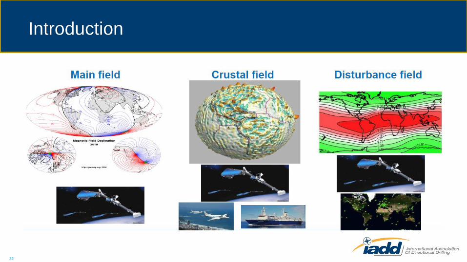
Introduction
32

Disturbance Field from Magnetosphere
33
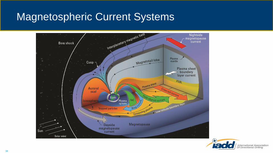
Magnetospheric Current Systems
34
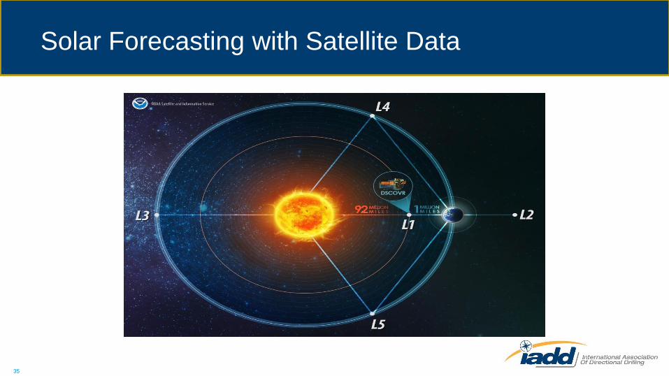
Solar Forecasting with Satellite Data
35

Real-time Prediction of Magnetospheric Fields
36

37
Disturbance Field from Ionosphere
±80 nT Variaions 100-200 nT Variations

Storm Measurements
38

MWD Calibration
39
MWD with HDGM
- Fixed reference
MWD with
HDGM-RT+DIFI
- Variable reference
- Better fit
Data provided by Schlumberger

EMAG2 Crustal Grid Update
40
Primary source of data
comes from marine and
airborne tracklines
• Over 100 institutions
• Over 50 years
• 3255 surveys
• 75.9 million data points
• 10.5 million miles
• Precompiled grids over
continental areas
• Provided by Governments,
Industry, and Academia

Send Us Your Data!
More data will enable a more detailed grid and more
accurate crustal field models
NOAA can offer long-term archival
Data can be flagged as private/proprietary (not for public
download); we currently archive proprietary data
Even decimated / lower-resolution datasets would be
useful
Contact us at [email protected]
41

424242
TECHNICAL PRESENTATIONSA New Approach to MWD Calibration to Improve Accuracy and
Reduce Calibration Time
Angus Jamieson, University of the Highlands and Islands
New Approach Objectives
Avoid orthogonality issues
Allow more sensors to be used
Make calibrations more accurate
Speed up calibration process
Improve MWD accuracy
43

Reference Angles
44
For Example
T W
X 0 90
Y 90 90
Z 0 0
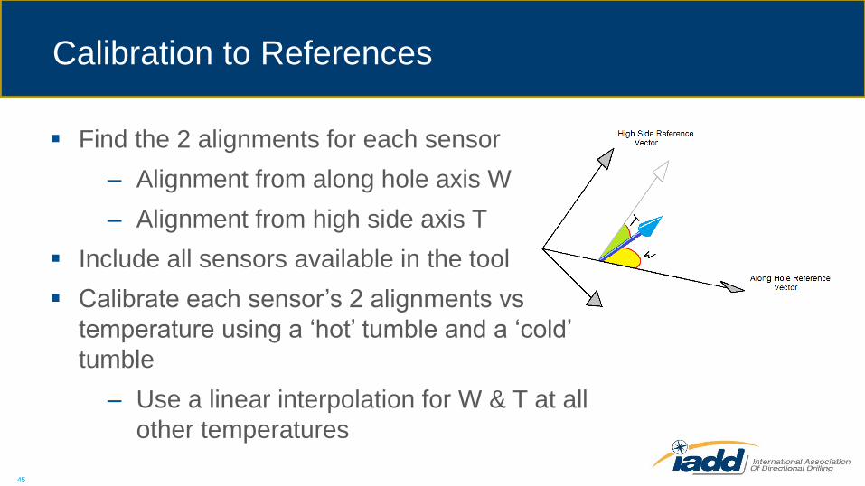
Calibration to References
45
Find the 2 alignments for each sensor
– Alignment from along hole axis W
– Alignment from high side axis T
Include all sensors available in the tool
Calibrate each sensor’s 2 alignments vs
temperature using a ‘hot’ tumble and a ‘cold’
tumble
– Use a linear interpolation for W & T at all
other temperatures

Calibration to References
Using actual alignments corrected at each temperature
– Set tool to Incl 60°, Azm 0°, Tool Face -45°, heat to 150°C and record while cooling
– Set tool to Incl 120°, Azm 180°, Tool Face 135°, heat to 150°C and record while cooling
– Determine least squares best fit polynomials to correct for scale and bias
In instrument firmware, use temperature corrected sensor data and actual alignments to produce synthetic 3-axis perfectly orthogonal data for surveys
46

Further Information
Detailed mathematics and procedure are in presentation
Program is available from Angus for calibrations of both
magnetometers and accelerometers
47
Advantages
Much shorter calibration time
Greater accuracy in the result
Uses all available sensors in the calculation of angles
Same process regardless of the number of sensors
Same output (perfectly orthogonal raw data or Incl, Azm,
and Tool Face)
No change to field procedures
48
494949
TECHNICAL PRESENTATIONSEast-West Exclusion Zones:
Why Do We Have Them and How Can We Eliminate Them?
Chad Hanak, Superior QC

50
Why Exclusion Zones?
Problem with Drilling East/West
Axial Magnetic Interference
(AMI)
50% more error than Declination
Available Corrections
Single Station Correction (SSC)
Multi-Station Analysis (MSA)
Problems with the Corrections
Multiple solutions
Degraded accuracy

Exclusion Zones for Horizontal Wells
Existing Standards
(SPE 125677)
BGGM
– 0.82 > sin(I)*sin(Az)
– ±35° from East/West
IFR1
– 0.91 > sin(I)*sin(Az)
– ±25° from East/West
51
BGGM Exclusion Zone

52
Multiple Solution Problem: SSC
Single Station Correction
Bx and By are measured
Bx and By are modeled as a
function of Azm using
– Reference Bt & Dip
– Measure Incl & TF
Minimum distance between
model and measurement is
found
(Bx, By) as a Function of Azm
53
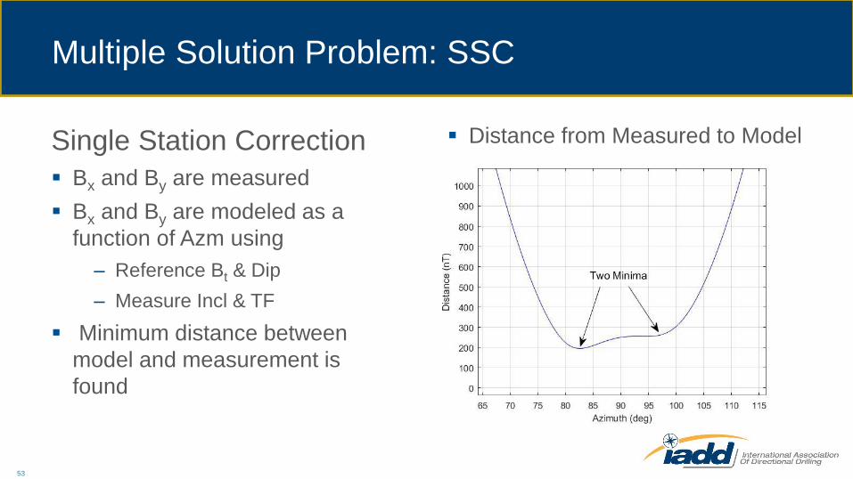
Multiple Solution Problem: SSC
Single Station Correction
Bx and By are measured
Bx and By are modeled as a
function of Azm using
– Reference Bt & Dip
– Measure Incl & TF
Minimum distance between
model and measurement is
found
Distance from Measured to Model

54
Multiple Solution Problem: SSC
How to handle?
Consider the uncertainty in
– Reference Bt
– Reference Dip
– Measured Incl
– Measured TF
Multiple Minima inside 3σ Uncertainty
55
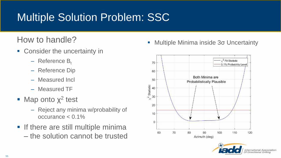
Multiple Solution Problem: SSC
How to handle?
Consider the uncertainty in
– Reference Bt
– Reference Dip
– Measured Incl
– Measured TF
Map onto χ2 test
– Reject any minima w/probability of
occurance < 0.1%
If there are still multiple minima
– the solution cannot be trusted
Multiple Minima inside 3σ Uncertainty
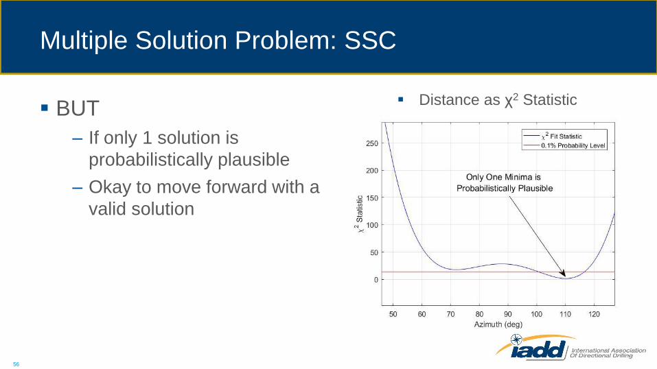
Multiple Solution Problem: SSC
BUT
– If only 1 solution is
probabilistically plausible
– Okay to move forward with a
valid solution
56
Distance as χ2 Statistic

Multiple Solutions: MSA
SSC was the EASY version
MSA similar – Multiple solutions can exist
– MSA does NOT automatically replace SSC in exclusion zone
– Variation in wellbore direction CAN resolve
– Required AMOUNT of variation is situation dependent
57

Degraded Accuracy
SSC
Correction not as accurate as standard MWD IPM near East/West
Specific IPM derived to model accuracy of correction (+AX)
Accounts for effects of magnetic reference field errors
MSA
+MS error model does not model the accuracy of MSA corrections
No published requirements to check for valid use
Best Option: Calculate accuracy directly for chosen solution
58

Drilling Safely East/West
If AMI corrections are required:
Check for multiple solutions
Ensure IPM assigned to
corrected surveys does not
overstate accuracy
59
MSA Exclusion Zone for Horizontal Wellbores: ±15°

60
Eliminating the Exclusion Zone
Including part of the build in the
lateral:
Start lateral at 80° Inclination
– Exclusion zone is ±5°
Start lateral at 70° Inclination
– Exclusion zone is eliminated
MSA Exclusion Zone with part of build included in lateral
Conclusions
Axial Magnetic Interference (AMI) creates large azimuthal errors when drilling East/West
SSC & MSA have problems
– Multiple solutions
– Degraded accuracy
Can reduce ±35° exclusion zone by
– Checking probabilistic plausibility of extra solutions
– Validating target IPM against calculated accuracy of corrections (MSA)
61

E-Book & Course
62
E-book
http://www.uhi.ac.uk/en/research-enterprise/wellbore-positioning-
download
Editorial Mangers:
David Gibson – Lodestar International
Carol Mann – DGI Graphics
Angus Jamieson – Univ Highlands and Islands
Steve Mullin – Independent
Robert Long – Baker Hughes

Links
63
Website OFFICIAL
www.ISCWSA.NET
SPE
http://connect.spe.org/wellborepositioning/home
LinkedIn- Open forum for discussion with industry leaders
http://connect.spe.org/WellborePositioning
If you would like to be added to the ISCWSA e-mail distribution list please contact
Chad Hanak, ISCWSA Secretary on:

646464
Thanks!
Let’s Get Drilling.