Is GARCH(1,1) as good a model as the Nobel

prize accolades would imply?1

Catalin Starica 2

First draft: 13 October 2003

This version: 2 November 2003

1This research has been supported by The Bank of Sweden Tercentenary Foundation.2Department of Mathematical Statistics, Chalmers University of Technology, S–412 96, Gothenburg,

Sweden. Email: starica@math.chalmers.se. Web page: www.math.chalmers.se/˜starica1

2

Abstract

This paper investigates the relevance of the stationary, conditional, parametric ARCH

modeling paradigm as embodied by the GARCH(1,1) process to describing and forecasting

the dynamics of returns of the Standard & Poors 500 (S&P 500) stock market index.

A detailed analysis of the series of S&P 500 returns featured in Section 3.2 of the Ad-

vanced Information note on the Bank of Sweden Prize in Economic Sciences in Memory

of Alfred Nobel reveals that during the period under discussion, there were no (statisti-

cally significant) differences between GARCH(1,1) modeling and a simple non-stationary,

non-parametric regression approach to next-day volatility forecasting. A second finding is

that the GARCH(1,1) model severely over-estimated the unconditional variance of returns

during the period under study.

For example, the annualized implied GARCH(1,1) unconditional standard deviation of

the sample is 35% while the sample standard deviation estimate is a mere 19%. Over-

estimation of the unconditional variance leads to poor volatility forecasts during the period

under discussion with the MSE of GARCH(1,1) 1-year ahead volatility more than 4 times

bigger than the MSE of a forecast based on historical volatility.

We test and reject the hypothesis that a GARCH(1,1) process is the true data generating

process of the longer sample of returns of the S&P 500 stock market index between March

4, 1957 and October 9, 2003. We investigate then the alternative use of the GARCH(1,1)

process as a local, stationary approximation of the data and find that the GARCH(1,1)

3

model fails during significantly long periods to provide a good local description to the time

series of returns on the S&P 500 and Dow Jones Industrial Average indexes.

Since the estimated coefficients of the GARCH model change significantly through time,

it is not clear how the GARCH(1,1) model can be used for volatility forecasting over

longer horizons. A comparison between the GARCH(1,1) volatility forecasts and a simple

approach based on historical volatility questions the relevance of the GARCH(1,1) dynam-

ics for longer horizon volatility forecasting for both the S&P 500 and Dow Jones Industrial

Average indexes.

JEL classification: C14, C16, C32.

Keywords and Phrases: stock returns, volatility, Garch(1,1), non-stationarities, uncon-

ditional time-varying volatility, IGARCH effect, longer-horizon forecasts.

4

1. Introduction

Even a casual look through the econometric literature of the last two decades reveals a

drastic change in the conceptual treatment of economic time series. The modeling of such

time series moved from a static set-up to one that recognizes the importance of fitting the

time-varying features of macro-economic and financial data.

In particular, it is now widely accepted that the covariance structure of returns (referred

often as volatility) changes through time. A large part of the modern econometric literature

frames modeling of time-varying volatility in the autoregressive conditional heteroskedastic

(ARCH) framework, a stationary, parametric, conditional approach that postulates that

the main time-varying feature of returns is the conditional covariance structure3 while as-

suming in the same time that the unconditional covariance remains constant through time

(see for example, the survey Bollerslev et al [4]). While the autoregressive conditional het-

eroskedastic approach to modeling time-varying volatility is currently prevalent, alternative

methodologies for volatility modeling exist in the econometric literature. In particular, the

non-stationary framework that assumes the unconditional variance to be the main time-

varying feature of returns has a long tradition that can be traced back to Officer [15], Hsu,

Miller and Wichern [11], Merton [12], French et al. [7].

This paper is motivated by the desire to better understand the relevance of the station-

ary, parametric conditional ARCH paradigm as embodied by the GARCH(1,1) process to

modeling and forecasting the returns of financial indexes. We focus on the GARCH(1,1)

3The conditional covariance structure is supposed to follow an autoregressive mechanism from where

the name of the paradigm.

5

process (Bollerslev [3], Taylor [17]) since this model is widely used and highly regarded in

practice as well as in the academic discourse. Producing GARCH(1,1) time-varying volatil-

ity estimates is part of the daily routine in many financial institutions. In the academic

literature, the GARCH(1,1) process seems to be perceived as a realistic data generating pro-

cess for financial returns. As a result, a large number of econometric and statistical papers

that develop estimation and testing techniques4 based on the assumption of a GARCH-

type data generating mechanism, use the GARCH(1,1) model to actually implement their

results.

The main goal of the paper is to investigate how close is the simple endogenous dynamics

imposed by a GARCH(1,1) process to the true dynamics of returns of main financial

indexes. To this end we analyze in detail the log-returns of the S&P 500 stock market

index between March 4, 1957 and October 9, 20035. Further evidence is brought in from

the analysis of the Dow Jones Industrial Average index covering the same period.

Our endeavor is, by nature, limited in scope. An analysis of the level of detail character-

izing ours cannot encompass, in the length of one paper, alternative ARCH-type models

and/or more series. Hence, the conclusions we draw are fortuitously limited to one model

4This includes testing of economic and financial theories like the Arbitrage Pricing Theory or the Capital

Asset Pricing Model.5The S&P 500 stock index took the present form of an average of the price of 500 stocks on March 4,

1957.

6

and two time series. However it is worth remembering that the model is the most cele-

brated member of the ARCH family while the time series represent the epitome of financial

return data.

The paper is organized as follows. Section 2 focuses on modeling and forecasting issues

related to the series of S&P 500 returns between May 16, 1995 to April 29, 2003. In Section

2.1 the stationary, parametric GARCH(1,1) model is compared to a simple non-stationary,

non-parametric regression approach in the context of next-day volatility forecasting. Sec-

tion 2.2 discusses the GARCH(1,1) estimated unconditional variance of returns during the

period under study. The impact of these estimates on GARCH(1,1) forecasting is analyzed

in Section 2.3.

Section 3 discusses modeling and forecasting issues related to the longer series of S&P

returns between March 4, 1957 and October 9, 2003. In section 3.1 we test the hypothesis

that a GARCH(1,1) process is the true data generating process of the longer sample of re-

turns on the S&P 500 and Dow Jones Industrial Average stock market indexes. In Section

3.2 we offer a possible explanation for the poor estimates of the unconditional volatility

documented in Section 2.2. We also evaluate the GARCH(1,1) process as a local stationary

approximation of the return data. In Section 3.3 a comparison between the GARCH(1,1)

volatility forecasts and a simple approach based on historical volatility evaluates the rele-

vance of the GARCH(1,1) dynamics for longer horizon volatility forecasting for both the

S&P 500 and Dow Jones Industrial Average indexes. Section 4 concludes.

7

2. The GARCH(1,1) model and the S&P 500 index returns between May

16, 1995 and April 29, 2003

When modeling the returns on the S&P 500 index in the stationary, parametric, condi-

tional ARCH framework, the working assumption is often that the data generating process

is the GARCH(1,1) model

(2.1) rt = zth1/2t , ht = α0 + α1 r2

t−1 + β1 ht−1,

where (zt) are iid, Ez = 0, Ez2 = 1. Since the GARCH(1,1) process is stationary, assuming

it as data generating process implicitly assumes that return data is stationary.

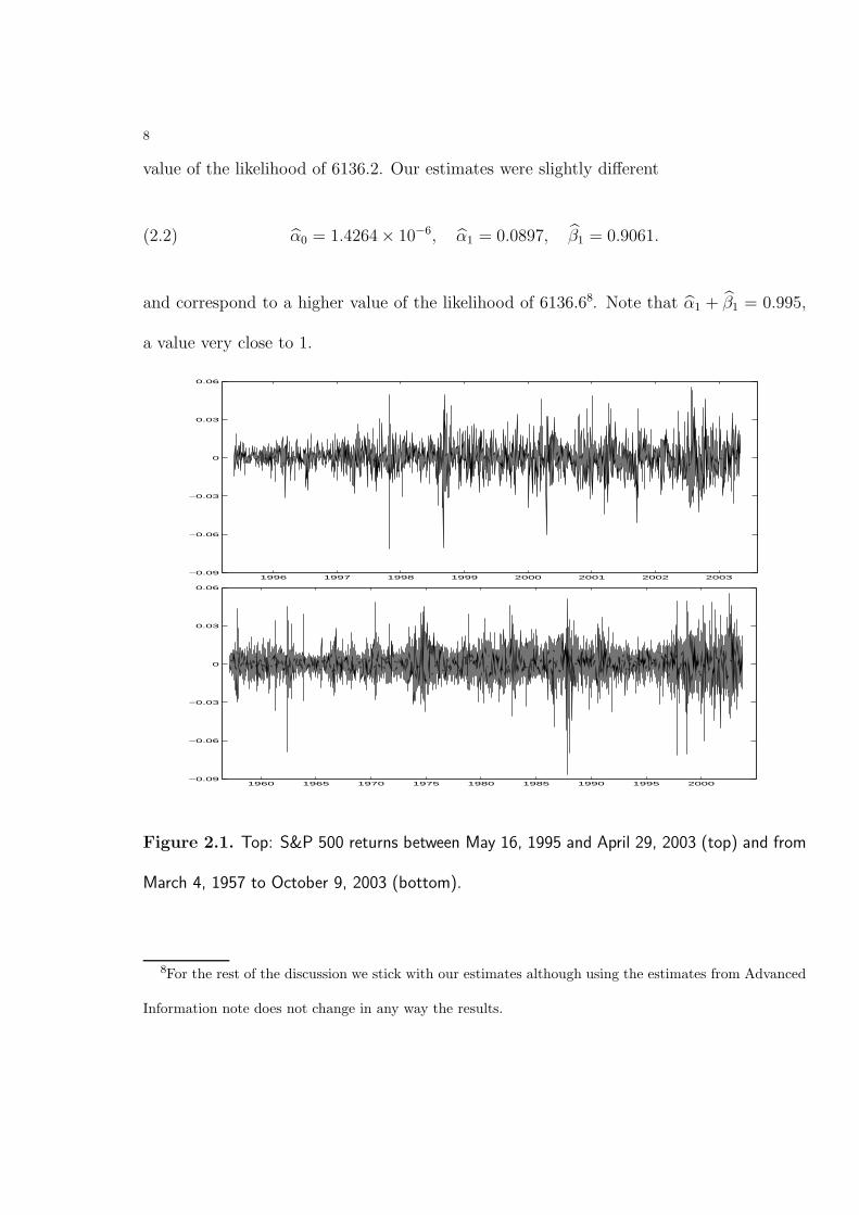
We begin with a detailed analysis of the series of S&P 500 returns between May 16,

1995 to April 29, 2003 - 2000 observations in all6. The upper panel of Figure 2.1 shows

the daily logarithmic returns (first differences of the logarithms of daily closing price) (on

the bottom row the longer sample of returns on the S&P 500 index from March 4, 1957

to October 9, 2003 is displayed7). According to the Advanced Information note, fitting a

conditionally normal GARCH(1,1) process to the series on the first row in Figure 2.1 yields

the estimated parameters α0 = 2 × 10−6, α1 = 0.091, and β1 = 0.899 corresponding to a

6This particular time series is featured in the illustration of the use of the GARCH(1,1) model in

estimating and forecasting volatility in Section 3.2 of the Advanced Information note on the Bank of

Sweden Prize in Economic Sciences in Memory of Alfred Nobel. The note is available as

http://www.nobel.se/economics/laureates/2003/ecoadv.pdf7Since most of the analyses in the sequel are done under the assumption of stationarity, the returns of

the week starting with 19 October 1987 were considered exceptional and were removed from the sample.

8

value of the likelihood of 6136.2. Our estimates were slightly different

(2.2) α0 = 1.4264 × 10−6, α1 = 0.0897, β1 = 0.9061.

and correspond to a higher value of the likelihood of 6136.68. Note that α1 + β1 = 0.995,

a value very close to 1.

1996 1997 1998 1999 2000 2001 2002 2003−0.09

−0.06

−0.03

0

0.03

0.06

1960 1965 1970 1975 1980 1985 1990 1995 2000−0.09

−0.06

−0.03

0

0.03

0.06

Figure 2.1. Top: S&P 500 returns between May 16, 1995 and April 29, 2003 (top) and from

March 4, 1957 to October 9, 2003 (bottom).

8For the rest of the discussion we stick with our estimates although using the estimates from Advanced

Information note does not change in any way the results.

9

2.1. Next-day volatility forecasting. One of the main achievements of the GARCH

modeling consists in providing accurate next-day volatility forecasts. Statistically, this

statement is supported by measures of the goodness of fit of the model (2.1) based on the

estimated innovations or residuals defined as:

(2.3) zt = rt/h1/2t , ht = α0 + α1 r2

t−1 + β1ht−1, t = 1, . . . , n.

Residuals that are close to being independent are taken as evidence of accurate next-day

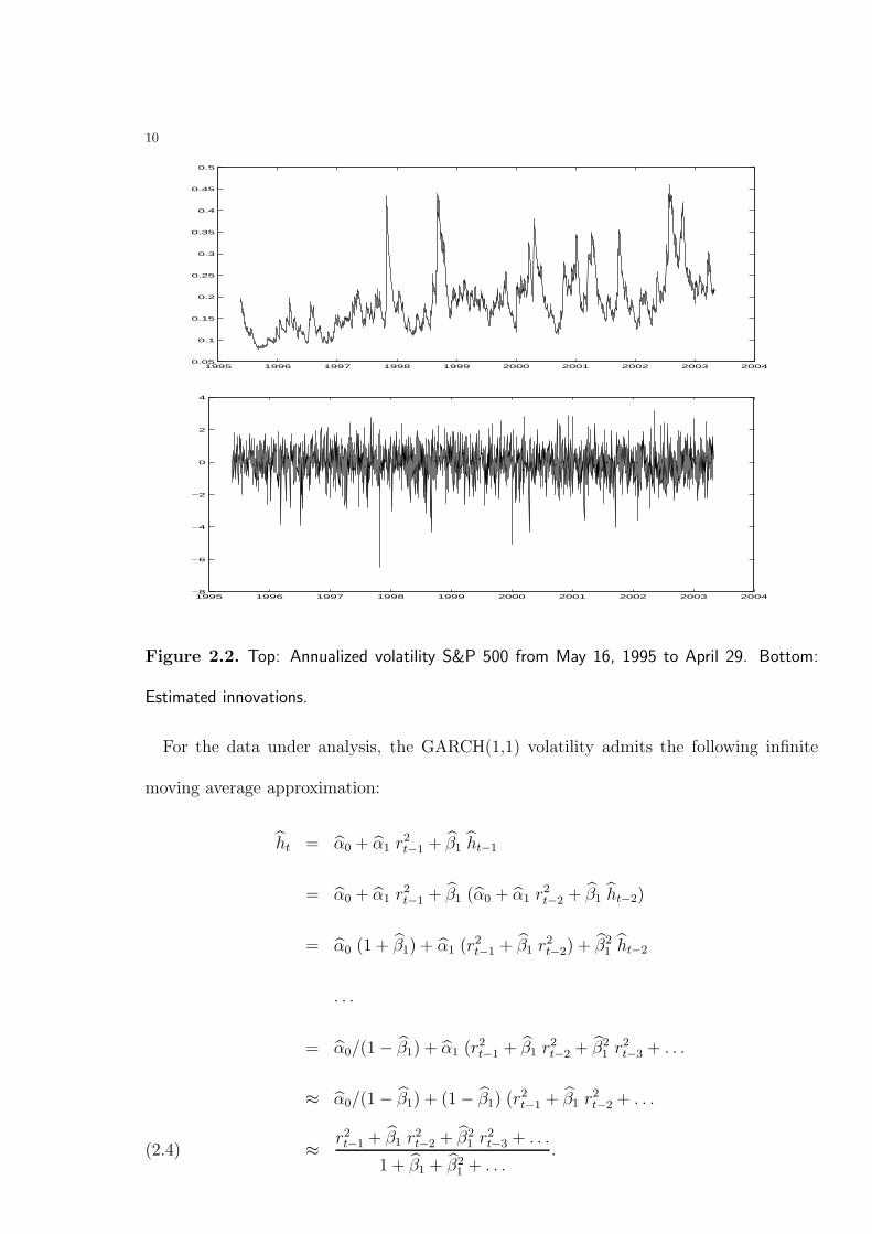
volatility forecasts. Figure 2.2 displays the estimated GARCH(1,1) volatility as well as

the residuals from the model (2.1) with parameters (2.2) corresponding to the period from

May 16, 1995 to April 29, 2003.

While the sample ACF of the absolute returns displays significant linear dependency at

lags as large as 100 (Figure 2.3–top), the absolute residuals pass the Ljung-Box test of

independence for at least the first 100 lags (Figure 2.3–bottom)(for more details on the

Ljung-Box test, see Brockwell and Davis [5]).

10

1995 1996 1997 1998 1999 2000 2001 2002 2003 20040.05

0.1

0.15

0.2

0.25

0.3

0.35

0.4

0.45

0.5

1995 1996 1997 1998 1999 2000 2001 2002 2003 2004−8

−6

−4

−2

0

2

4

Figure 2.2. Top: Annualized volatility S&P 500 from May 16, 1995 to April 29. Bottom:

Estimated innovations.

For the data under analysis, the GARCH(1,1) volatility admits the following infinite

moving average approximation:

ht = α0 + α1 r2t−1 + β1 ht−1

= α0 + α1 r2t−1 + β1 (α0 + α1 r2

t−2 + β1 ht−2)

= α0 (1 + β1) + α1 (r2t−1 + β1 r2

t−2) + β21 ht−2

. . .

= α0/(1 − β1) + α1 (r2t−1 + β1 r2

t−2 + β21 r2

t−3 + . . .

≈ α0/(1 − β1) + (1 − β1) (r2t−1 + β1 r2

t−2 + . . .

≈ r2t−1 + β1 r2

t−2 + β21 r2

t−3 + . . .

1 + β1 + β21 + . . .

.(2.4)

11

0 10 20 30 40 50 60 70 80 90 100−0.1

0

0.1

0.2

0.3

0.4

0 20 40 60 80 100

−0.08

−0.06

−0.04

−0.02

0

0.02

0.04

0.06

0.08

0 20 40 60 80 1000

0.2

0.4

0.6

0.8

1

lag

Ljung−

Box p−

value

Figure 2.3. Sample ACF of absolute values of returns (top) and of absolute values of residuals

(bottom-left). The p-values of the Ljung-Box statistic for the absolute values of the residuals

(bottom-right). The hypothesis of independence is rejected for small p-values.

The first approximation consists in replacing α1 with 1− β1 (recall that α1 + β1 = 0.995)

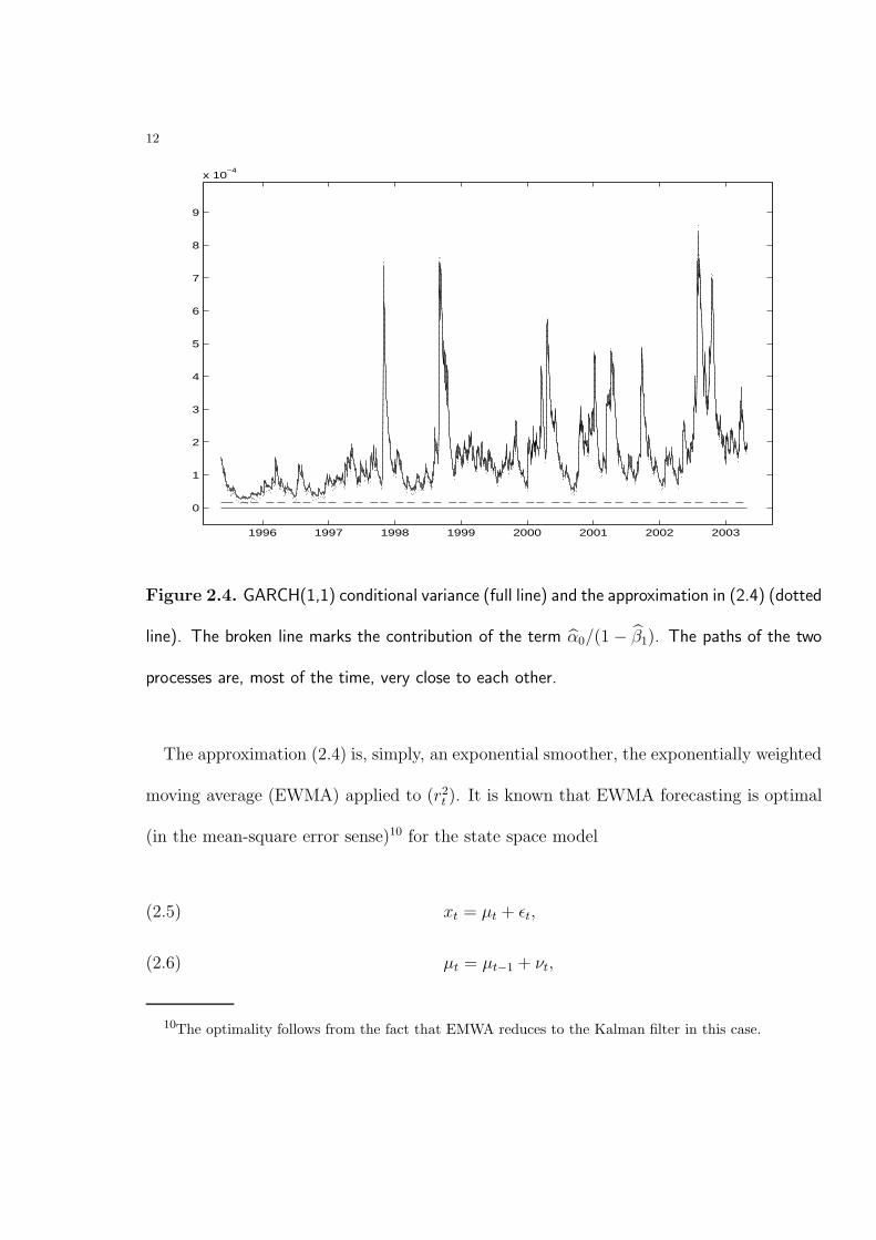
while the second one neglects the term α0/(1 − β1)9. Figure 2.4 displays the conditional

variance process as well as its approximation given by (2.4) and show a close correspondence

between the two processes.

9While more important during the low volatility period up to the beginning of 1997, this term accounts

on average, for 10% of the variance during the period 1997-2003.

12

1996 1997 1998 1999 2000 2001 2002 2003

0

1

2

3

4

5

6

7

8

9

x 10−4

Figure 2.4. GARCH(1,1) conditional variance (full line) and the approximation in (2.4) (dotted

line). The broken line marks the contribution of the term α0/(1 − β1). The paths of the two

processes are, most of the time, very close to each other.

The approximation (2.4) is, simply, an exponential smoother, the exponentially weighted

moving average (EWMA) applied to (r2t ). It is known that EWMA forecasting is optimal

(in the mean-square error sense)10 for the state space model

xt = µt + εt,(2.5)

µt = µt−1 + νt,(2.6)

10The optimality follows from the fact that EMWA reduces to the Kalman filter in this case.

13

where (εt) and (νt) are iid sequences, Eε = 0, Eν = 0. In the state space model set-up,

equation (2.6) incorporates the uncertainty about the form of the model.

Note that the GARCH(1,1) model can be written in the form of equation (2.5):

r2t = ht + ht(z

2t − 1) := ht + εt,

with Eε = 0. Going one step further,11 equation (2.6) would translate to

(2.7) ht = ht−1 + νt.

In words, equation (2.7) acknwoledges that the dynamic of the variance is unpredictable.

While a small variance of the noise ν can imply that the daily changes are so small as to

be ignored, over longer periods of time the movements of the variance cannot be foreseen

hence modeled.

A closely related set-up, subtly different but which shares with the state model repre-

sentation the ability to incorporate our uncertainty about the form of the model is that

of the non-parametric regression (see for example, Wand and Jones [18]). The mentioned

uncertainty is handled in this case by modeling the signal µ as a deterministic function of

time12

xt = µ(t) + εt,(2.8)

11The discussion here is purely at a formal level. No modeling will be done in the space state set-up.

Instead a closely related framework to address the uncertainty of the model will be used. Had we pursued

the state space specification, special care would have been needed to asssure that ht stays positive

12In both situations the local level or the local trend can be estimated as well as desired.

14

where (εt) is an iid sequence, Eε = 0.

This association suggests the following simple non-parametric, non-stationary alternative

approach. Assume that

rt = σ(t) εt, Eε = 0, Eε2 = 1.(2.9)

where σ(t) is a deterministic, smooth function of time. In words, assume that the uncon-

ditional variance is time-varying and that the returns are independent (but of course, not

identically distributed). Rewrite equation (2.9) in the form of (2.8)

r2t = σ2(t) + σ2(t)(ε2

t − 1) := σ2(t) + εt, Eε = 0.(2.10)

Following the non-parametric regression literature (see for example, Wand and Jones

[18]), an estimate of the time-varying unconditional variance σ2(t) is given by

σ2(t; b) =

n∑k=1

Wk(t; b) r2k(2.11)

where b is the bandwidth and the weights Wk are given by

Wk(t; b) = K

(k − t

b

)/

n∑k=1

K

(k − t

b

),(2.12)

where K is a kernel (for details on the definition and the properties of a kernel function

see the reference above). The expressions (2.11), (2.12) are the Nadaraya-Watson, or zero-

degree local polynomial, kernel estimate.

The specific of the problem at hand is that we want to forecast the next-day volatility,

i.e. use the return data available at time t − 1 to forecast σ(t). This is accomplished by

the right choice of a kernel in (2.12). More concretly, the kernel K will be a half-kernel or

15

a one-sided kernel, i.e. K(x) = 0 for x ≥ 0. This implies that Wk(t; b) = 0 if k ≥ t. With

this choice of a kernel, equation (2.11) yields the forecasted time-varying variance

σ2(t; b) =

t−1∑k=1

K

(k − t

b

)r2k/

t−1∑k=1

K

(k − t

b

).(2.13)

In the sequel we use the exponential and the normal half-kernels as illustrations. Note

that σ2(t; b), the estimated time-varying unconditional variance at time t depends only on

information prior to this moment, i.e. only the returns up to time t− 1 have been used in

estimation.

0 10 20 30 40 50 60 706.4

6.6

6.8

7

7.2

7.4

7.6

7.8

8

8.2

8.4

x 10−8

0 10 20 30 40 50 60 706.4

6.6

6.8

7

7.2

7.4

7.6

7.8

8

8.2

8.4

x 10−8

Figure 2.5. The average of the squared residuals (ASR) defined in (2.14) as a function of b

for the two choices of kernel: the exponential (on the left) and the normal (on the right). A

minimum is attained at bexpASR = 11 and bnormal

ASR = 12, respectively.

The key quantity in the non-parametric regression is b, the bandwidth. From the plethora

of methods proposed in the extensive statistical literature on the bandwidth selection (see

for example Gasser et al. [8]), the simplest one takes b to minimize the average of the

16

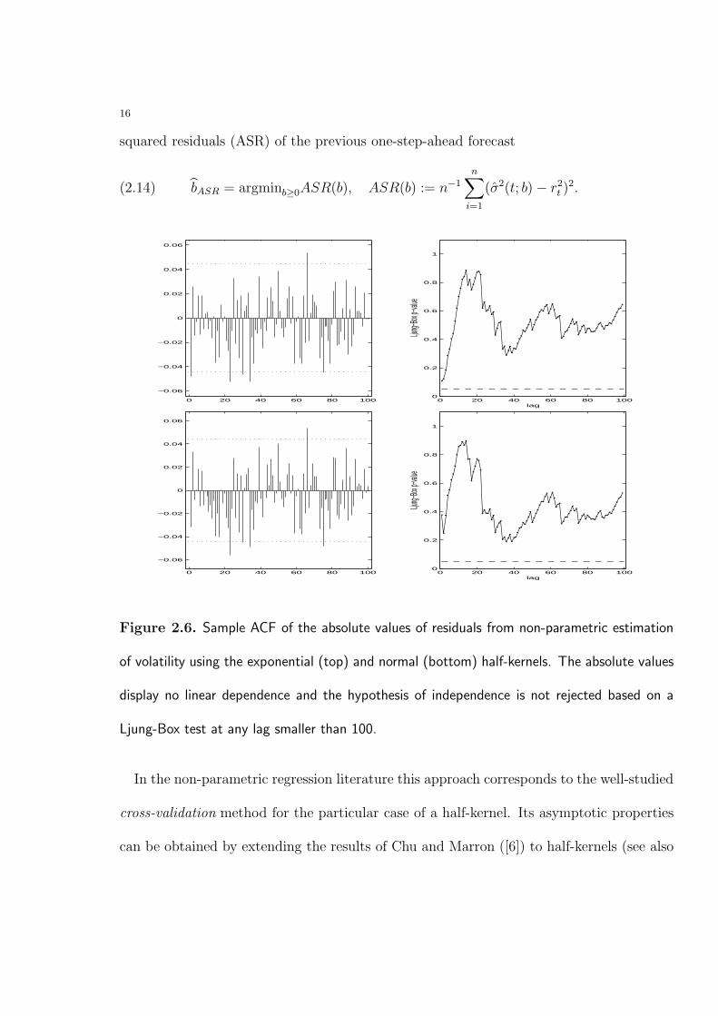
squared residuals (ASR) of the previous one-step-ahead forecast

bASR = argminb≥0ASR(b), ASR(b) := n−1n∑

i=1

(σ2(t; b) − r2t )2.(2.14)

0 20 40 60 80 100

−0.06

−0.04

−0.02

0

0.02

0.04

0.06

0 20 40 60 80 1000

0.2

0.4

0.6

0.8

1

lag

Ljung−

Box p−

value

0 20 40 60 80 100

−0.06

−0.04

−0.02

0

0.02

0.04

0.06

0 20 40 60 80 1000

0.2

0.4

0.6

0.8

1

lag

Ljung−

Box p−

value

Figure 2.6. Sample ACF of the absolute values of residuals from non-parametric estimation

of volatility using the exponential (top) and normal (bottom) half-kernels. The absolute values

display no linear dependence and the hypothesis of independence is not rejected based on a

Ljung-Box test at any lag smaller than 100.

In the non-parametric regression literature this approach corresponds to the well-studied

cross-validation method for the particular case of a half-kernel. Its asymptotic properties

can be obtained by extending the results of Chu and Marron ([6]) to half-kernels (see also

17

Gijbels et al. [9]). Figure 2.5 displays the ASR as a function of b for two choices of kernel:

the exponential (on the left) and the normal (on the right). Both graphs have a convex

shape attaining a minimum at bexpASR = 11 and bnormal

ASR = 12, respectively13.

Figure 2.6 displays the sample ACF of the residuals from the non-parametric regression

(2.15) εt = rt/σ(t; bASR), t = 1, . . . , n.

The residuals show no linear dependence and the hypothesis of independence is not rejected

based on a Ljung-Box test at any lag smaller than 100.

Figure 2.7 displays the GARCH(1,1) volatility together with the non-parametric estimate

(2.13) with a normal half-kernel. The paths of the two volatility processes follow each other

closely.

1996 1997 1998 1999 2000 2001 2002 20030

0.1

0.2

0.3

0.4

Figure 2.7. (Annualized) Volatility estimates: GARCH(1,1) version (full line) and the non-

parametric regression estimate (2.13) with a normal half-kernel (doted line). The paths of the

two volatility processes are, most of the time, very close.

13In the notation of equation (2.4), the value bexpASR = 11 corresponds to a β = 0.91.

18

The evidence presented shows that, during the period under discussion, there were no

(statistically significant) differences between GARCH(1,1) and a simple non-stationary,

non-parametric regression approach to next-day volatility forecasting.

An objection against the non-parametric framework outlined above could be that it lacks

any dynamics and would be embodied by the question: What has this approach to say

about the future?14. Furthermore, one could argue that, by contrast, the GARCH(1,1)

model, by specifying a certain endogenous mechanism for the volatility process, is capable

to foresee future developments in the movements of prices. Shortly, the GARCH(1,1) model

is preferable because it has a vision of the future.

In the sequel we will analyze the relevance of this possible objection/argument from

a number of different perspectives. First we will discuss some modeling and forecasting

implications of postulating a GARCH(1,1) volatility mechanism on the returns between

May 16, 1995 to April 29, 2003 (sections 2.2 and 2.3). Then we will take a closer look at

the relevance of the GARCH(1,1) dynamics for the longer S&P 500 sample covering the

period between March 4, 1957 and October 9, 2003 (sections 3.1, 3.2). Finally, both the

14The answer to this question, that might not fully satisfy the ones in favor of tight parametric modeling,

is: since we assume that the volatility is driven by exogenous factors (that are hard to identify and hence

we leave unspecified), i.e. we do not know if it will move up or down, and that it evolves smoothly and

slowly, i.e. it will take a while until significant changes will be noticed, the best we can do is to accurately

measure the current level and to forecast it as the return volatility for the close future. The near future

returns will be modeled as iid with a variance equal to today’s estimate.

19

GARCH(1,1) methodology and the non-parametric regression approach will be considered

in the frame of longer horizon volatility forecasts in section 3.3.

2.2. Modeling performance. As mentioned earlier, a common working assumption in

the financial econometric literature is that the GARCH(1,1) process (2.1) is the true data

generating process for financial returns. Under such an assumption and given a data sam-

ple, a GARCH(1,1) process with parameters estimated on a reasonably long subsample15

of the data should provide a good model for the whole sample. More concretely, the

GARCH(1,1) process with parameters (2.2) estimated on the 2000 observation long sub-

sample16 displayed on the top of Figure 2.1 should provide a reasonable description also for

the 11727 observation long sample on the bottom of the same figure17. To check if this is

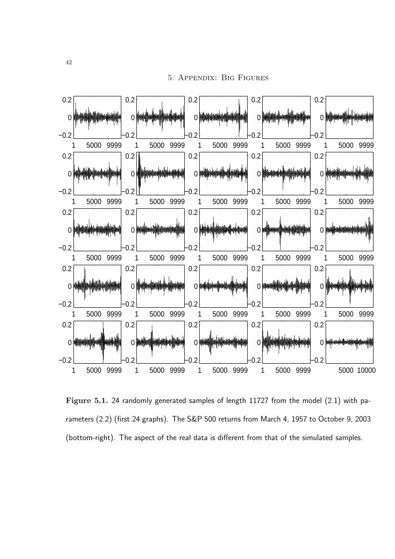
the case, we display in Figure 5.1 24 randomly generated samples of length 11727 from the

model (2.1) with parameters (2.2) together with the plot of the true return series. Note

that the over-all aspect of the simulated samples is quite different from that of the real

data.

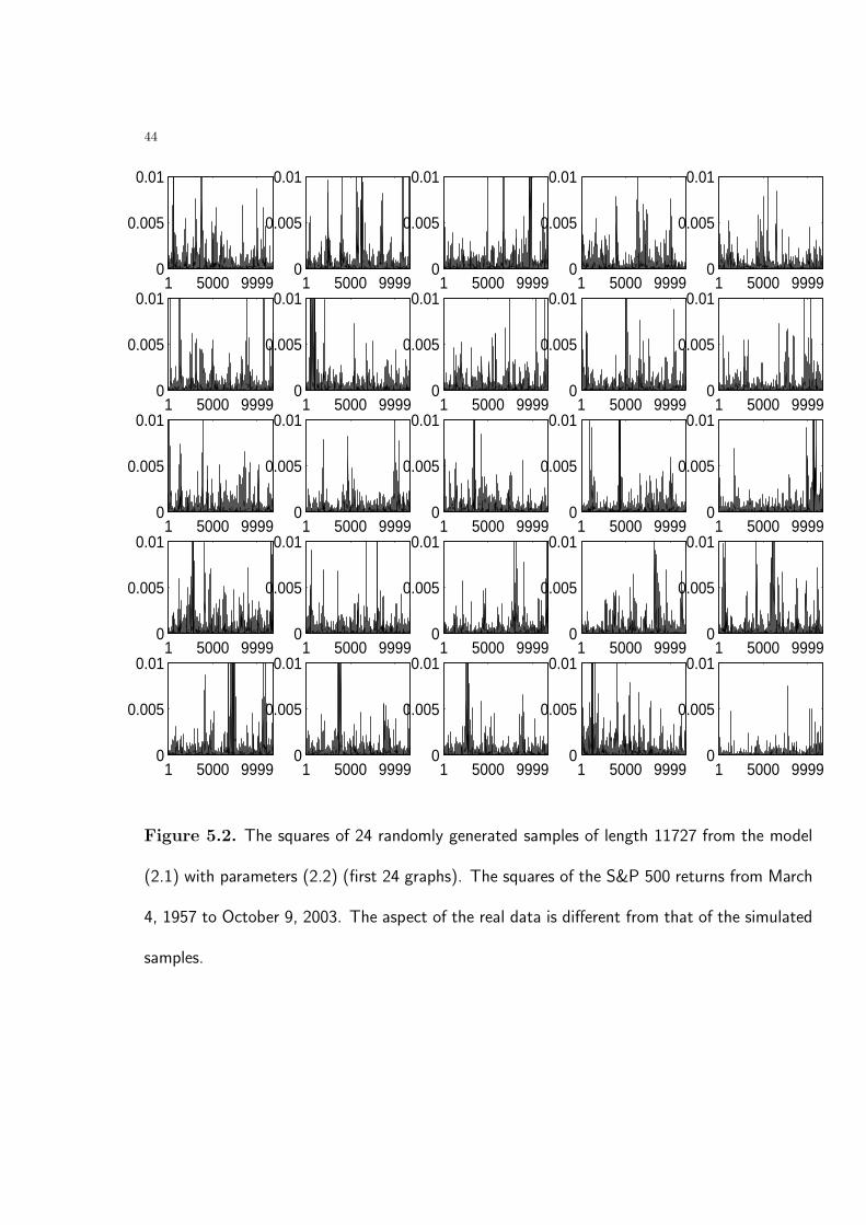
Figure 5.2 displays the squared values of the samples in Figure 5.1. Differences between

the aspect of the simulated samples and that of the return series are strongly visible. In

particular, the variance of the real data appears to be smaller.

15The subsample size should guarantee that the estimation error is likely to be small.16A sample size of 2000 is commonly assumed to be sufficient for a precise estimation of a GARCH(1,1)

model.

1711727 is the the length of the sample from March 4, 1957 to October 9, 2003.

20

The visual impression from Figure 5.1 and 5.2 is confirmed by simulations. The support

of the simulated18 distribution of the sample variance for samples of length 11727 from the

model (2.2) was the interval [0.00014,0.01526]. The value of the variance of the returns in

Figure 2.1 (bottom graph) is 0.00008.

This simple simulation exercise highlights the need for a closer look at the GARCH(1,1)

estimated unconditional variance. The model (2.1) was first estimated on the subsample

from May 16, 1995 to April 30, 1999 (the first 1000 observations in the sample) and then re-

estimated every 5 days on a sample that contains all past observations, i.e. all observations

between May 16, 1995 and the date of the re-estimation. Under the assumption of weak

stationarity, i.e. α1 + β1 < 1, the unconditional variance of the GARCH(1,1) model (2.1)

is given by

(2.16) σ2 := α0/(1 − α1 − β1).

Figure 2.8 displays the annualized estimated unconditional GARCH(1,1) standard devi-

ation (sd) together with the annualized sample sd, i.e. the square root of 250 times the

average of square returns from May 16, 1995 to current time location. The graph shows a

sd from 1.5 to 5 times bigger than the sample sd19. Hence, during the period under dis-

cussion, the unconditional variance point estimates of a GARCH(1,1) model are severely

out-of-line with the sample point estimates of the unconditional variance of returns.

1825.000 samples were simulated.19For example, the parameter values in the Advanced Information note imply an annualized sd of 35%

while the sample annualized sd is of merely 19%.

21

2000 2001 2002 20030.1

0.2

0.3

0.4

0.5

0.6

Figure 2.8. Estimated GARCH (1,1) sd (2.16) (dotted line) together with sample sd (both

estimates are annualized) (full line). The model (2.1) is re-estimated every 5 days on a sample

that contains all past observations beginning from May 16, 1995. The time mark corresponds to

the end of the sub-sample that yields the two sd estimates. The graph shows a big discrepancy

between the two estimates.

Since for the model (2.1) the volatility forecast at longer horizons is, practically, the

unconditional variance (see equation (2.17)), failing to produce accurate point estimates

for this last quantity will, most likely, produce poor longer horizon volatility forecasts. We

will now investigate this issue.

2.3. Forecasting performance. Let us now evaluate the out-of-sample forecasting per-

formance of the GARCH(1,1) model based on the sample on top of Figure 2.1.

22

Assuming a GARCH(1,1) data generating process (2.1) that also satisfy20 α1 + β1 < 1,

it follows that the minimum Mean Square Error forecast for Er2t+p, the return variance

h-steps ahead, is

(2.17) σ2, GARCHt+p := Etr

2t+h = σ2 + (α1 + β1)

p(ht − σ2),

where σ2 is the unconditional variance defined in (2.16). Note that, since α1 + β1 < 1, for

large h, the forecast σ2, GARCHt+p is the unconditional variance, σ2.

The minimum MSE forecast for E(rt+1+. . .+rt+p)2, the variance of the next p aggregated

returns, is then given by

(2.18) σ 2, GARCHt,p := Et(rt+1 + . . . + rt+p)2 = σ2, GARCH

t+1 + · · · + σ2, GARCHt+p .

We take as benchmark (BM) for volatility forecasting the simple non-stationary model

(2.9). Since no dynamics is specified for the variance, future observations rt+1, rt+2, . . . are

modeled as iid with constant variance σ2(t), an estimate of σ2(t). In the sequel we use the

sample variance of the previous year of returns as the estimate for σ2(t). The forecast for

Er2t+p is then given by

(2.19) σ2, BMt+p := Er2

t = σ2(t),

20If this condition is not fulfilled, the GARCH(1,1) process, if stationary, has infinite variance.

23

2000 2001 20020.15

0.2

0.25

0.3

0.35

0.4

0.45

Figure 2.9. The (future) realized sd (annualized) at horizon 250 (full line) together with

GARCH forecast (broken line) and the benchmark (dotted line). The time mark is the beginning

of the period over which the forecast is made.

The forecast for E(rt+1 + . . . + rt+p)2, the variance of the next h aggregated returns is

simply

(2.20) σ 2, BMt,p := p σ2(t) =

p

250

250∑i=1

r2t−i+1.

The GARCH(1,1) model is estimated initially on the first 1000 data points corresponding

to the interval from May 16, 1995 to April 30, 1999, and re-estimated every 5 days (every

week). Contemporaneously, σ2(t) is estimated as the average of past 250 square returns.

After every re-estimation, volatility forecasts are made for the year to come (p = 1, . . . , 250)

using (2.18) and (2.20). The data used in the out-of-sample variance forecasting comparison

covers the interval May 3, 1999 to April 29, 2003.

24

0 50 100 150 200 2500.5

1

1.5

2

2.5

3

3.5

4

4.5

5

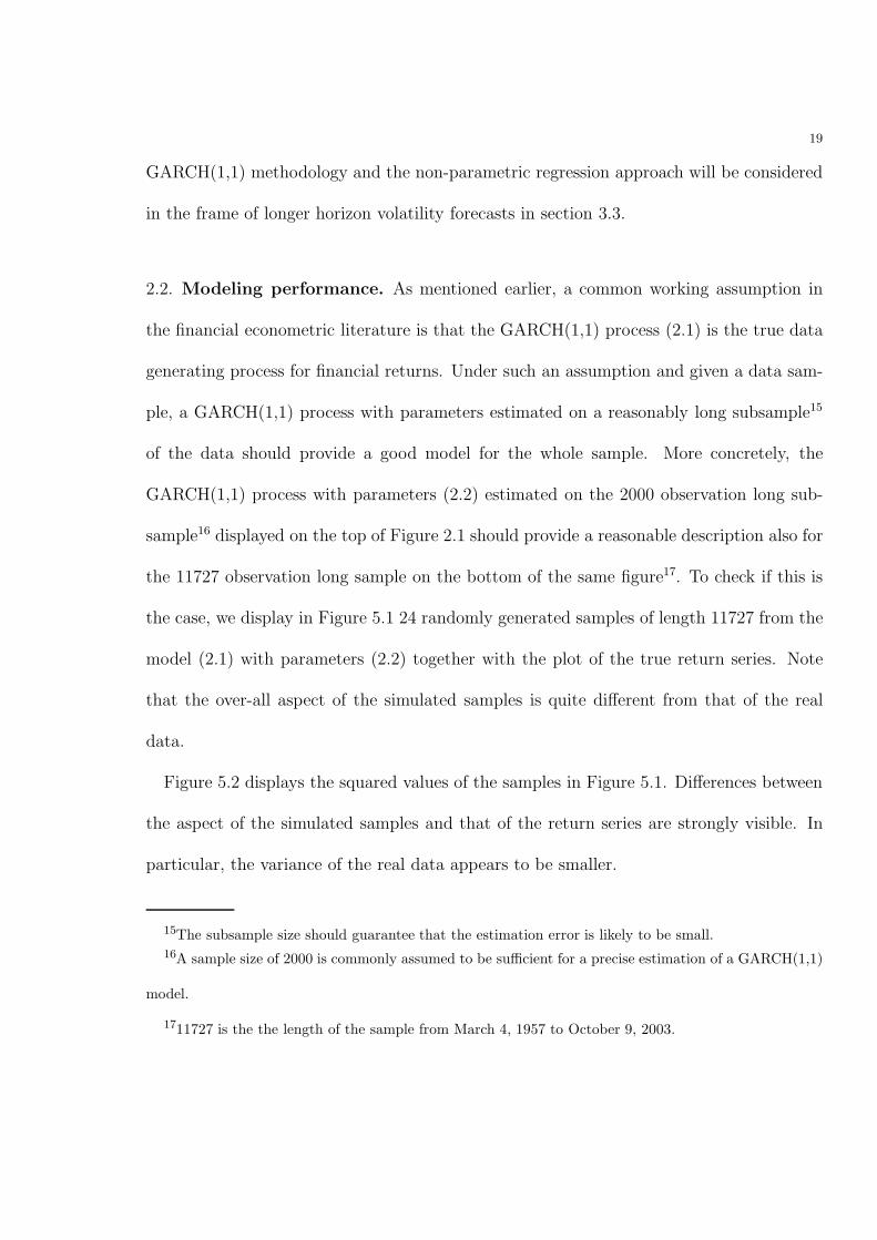
Figure 2.10. The ratio MSEGARCH/MSEBM . The MSE∗ are defined in (2.22). On the

x-axis, h, the forecast horizon.

Define the following measure of the realized volatility in the interval [t+1, t+p]

(2.21) r 2t,p :=

h∑i=1

r2t+i,

We calculated and compared the following MSE

(2.22) MSE∗(p) :=n∑

t=1

(r 2t,p − σ 2, ∗

t,p )2

with ∗ standing for BM or GARCH. The MSE (2.22) is preferred to the simpler MSE

n∑t=1

(r2t+p − σ2, ∗

t+p)2

25

since this last one uses a poor measure of the realized return volatility21. Through averaging

some of the idiosyncratic noise in the daily squared return data is canceled yielding (2.21),

a better measure against which to check the quality of the two forecasts.

Figure 2.9 shows the extent of the impact on forecasting of the over-estimation of un-

conditional variance illustrated in Figure 2.8. Note also the similarity of the shape of the

GARCH curves in Figure 2.8 and Figure 2.9.

Both Figure 2.10 and 2.9 show that a simple model with a time-varying uncondi-

tional variance (hence non-stationary) produced better out-of-sample forecasting than the

GARCH(1,1) model in the period May 3, 1999 to April 29, 2003.

In this section, we have seen that the GARCH(1,1) process produced point estimates of

the unconditional variance that were severely out-of-line with the sample point estimates

during the period May 3, 1999 to April 29, 2003. As a consequence, during this period

the model yielded poor longer horizon forecasts. The analysis we just concluded raises a

number of questions. Does the GARCH(1,1) process always over-estimate unconditional

variances? Or was the period we analyzed a special one? And if yes, in what way? To

answer these questions we performed a detailed analysis of the fit of the GARCH(1,1) on

the time series of returns of the S&P 500 index between March 4, 1957 and October 9,

2003. The results are presented in the next section.

21It is well known (see Andersen and Bollerslev [1]) that the realized square returns are poor estimates

of the day-by-day movements in volatility, as the idiosyncratic component of daily returns is large.

26

3. The GARCH(1,1) model and the S&P 500 index returns between March

4, 1957 and October 9, 2003

We begin with a re-examination of the working assumptions of the previous analysis.

The fact that the GARCH(1,1) process is a stationary model22 raises up front a method-

ological choice since one uses the GARCH(1,1) model differently, depending on the working

assumptions one is willing to make about the data to be modeled. Were the econometri-

cian convinced that the data is stationary, she would assume that a GARCH(1,1) process

is the true data generating process and she would estimate a GARCH(1,1) model on the

whole data set. She would try always to use as much data as possible in order to support

any statistical statement or to make forecasts. Had she reasons to believe that the data is

non-stationary, then the stationary GARCH(1,1) process could possibly become a useful

local approximation of the true data generating process. The parameters of the model

should then be re-estimated periodically on a moving window. Also she would shy away

from making statistical statements based on long samples and in forecasting she would

prefer to use the most recent past for the calibration of the model. However, were the data

unconditional features time-varying, it is not clear of what help would the GARCH(1,1)

model then be in producing volatility forecasts over longer horizons.

As we see, the two working assumptions on the nature of the data at hand have very

different methodological implications both on the estimation of the GARCH(1,1) model as

22The stationarity is central to issues of statistical estimation and of forecasting.

27

well as on its use in forecasting. In the sequel we investigate in detail the behavior of the

GARCH(1,1) model in the two outlined frameworks.

3.1. Working hypothesis: The returns are stationary. The GARCH(1,1) is the

true data generating process. The working assumption in this section will be that

the returns on the S&P 500 index between March 4, 1957 and October 9, 2003 form a

stationary time series . In this set-up one can test the hypothesis that a given parametric

model is the data generating process of this time series. More concretely, the estimated

parameters of such a model should be statistically the same no matter what portion of the

data is used in estimation. In particular, the parameters should be statistically identical

were they estimated on an increasing sample or on a window that moves through the data.

Detection of significant changes in the values of the estimated parameters leads to rejecting

the parameter model as the data generating process.

A GARCH(1,1) process was fit to the S&P 500 series of returns between March 4, 1957

and October 9, 2003 yielding the following parameters

(3.1) α0 = 4.78 × 10−7, α1 = 0.0696, β1 = 0.9267.

To evaluate the suitability of a GARCH(1,1) model as data generating process for the

S&P 500 return series, the model (2.1) was initially estimated on the first 2000 observations

of the sample in Figure 2.1 (bottom) corresponding roughly to the period 1957-1964. Then

the model was re-estimated every 50 observations both on a sample containing 2000 past

observations and on a sample containing all past observations. The results of the estimation

28

1965 1970 1975 1980 1985 1990 1995 2000

2

3

4

5

6

7

1965 1970 1975 1980 1985 1990 1995 2000

2

3

4

5

6

7

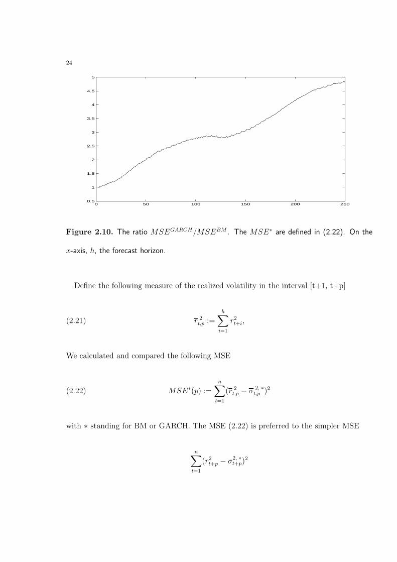
Figure 3.1. Estimated fourth moment of the residuals z for S&P 500 data. The model was

initially estimated on the first 2000 observations of the sample corresponding roughly to the

period 1957-1964, then re-estimated every 50 observations on a sample containing 2000 past

observations (left) and all past observations (right).

are displayed in Figure 5.3. The confidence intervals correspond to the quasi-maximum

likelihood (QML) estimation method and take into account possible misspecifications of

the conditional distribution (Gourieroux [10], Berkes et al. [2], Straumann and Mikosch

[16]). The graphs in Figure 5.3 show pronounced instability of the estimated values of the

parameters.

The asymptotic normality of the QML estimators depends on the existence of the finite

fourth moment for the distribution of the innovations z (assumption N3 of Theorem 7.1

Straumann and Mikosch [16]). Figure 3.1 displays the fourth moment of the estimated

residuals for the S&P 500 data together with the 95% confidence intervals (under the

assumption of independent innovations) and seems to confirm that the forth moment of

the innovations is finite.

29

A similar picture emerges from analyzing the returns on the Dow Jones Industrial stock

index. The evolution of the estimated GARCH(1,1) coefficients displayed in Figure 5.4

follow a similar pattern to the one in Figure 5.3.

0 1 2 3 4 5 6 7 8 9 100

0.1

0.2

0.3

0.4

0.5

0.6

0.7

0.8

0.9

1

0 1 2 3 4 5 6 7 8 9 10−5

−4

−3

−2

−1

0

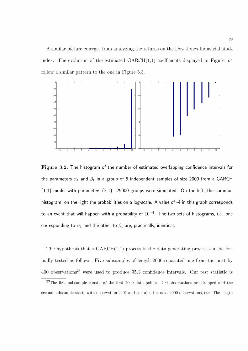
Figure 3.2. The histogram of the number of estimated overlapping confidence intervals for

the parameters α1 and β1 in a group of 5 independent samples of size 2000 from a GARCH

(1,1) model with parameters (3.1). 25000 groups were simulated. On the left, the common

histogram, on the right the probabilities on a log-scale. A value of -4 in this graph corresponds

to an event that will happen with a probability of 10−4. The two sets of histograms, i.e. one

corresponding to α1 and the other to β1 are, practically, identical.

The hypothesis that a GARCH(1,1) process is the data generating process can be for-

mally tested as follows. Five subsamples of length 2000 separated one from the next by

400 observations23 were used to produce 95% confidence intervals. Our test statistic is

23The first subsample consist of the first 2000 data points. 400 observations are dropped and the

second subsample starts with observation 2401 and contains the next 2000 observations, etc. The length

30

the number of pairs of overlapping confidence intervals. Under the null of a common

GARCH(1,1) data generating process, the test statistic should be close to 10. A small

number of overlapping pairs constitute evidence against the null. For parameter α1, 2

out of the 10 possible pairs of confidence intervals do overlap, while for parameter β1 the

number of overlapping pairs is 4. The probability of this two events, i.e. the probability of

observing less than m overlapping confidence intervals out of 10 possible pairs, m = 2 and

m = 4, can be bounded as follows. The probability that two 100×α% confidence intervals

overlap is greater than the probability that both the intervals contain the true parameter,

i.e. α2. Assuming that the actual coverage of the confidence intervals in Figure 5.3 is the

theoretical one24, i.e. 95%, the probability of seeing less than or 2 overlapping intervals out

10 possible pairs can be easily calculated as being at most 3 × 10−7 while the probability

of the separating blocks was chosen such that it maximizes the distance between the subsamples, yielding

nevertheless 5 non-overlapping series. 2 consecutive samples were separated by more than one year and a

half of data to guarantee that the assumption of independent subsamples is likely to be reasonable.24The test based on the confidence intervals of parameter α1 still rejects the null hypothesis at 5% if

the actual level of coverage is in fact as low as 71% and at 1% if the actual level is of 78% or higher. The

test based on the confidence intervals of parameter β1 rejects the hypothesis of stationarity at 5% if the

actual level of coverage is in fact as low as 84% and at 1% if the actual level is of 88% or higher. Note

that this calculations yield rather conservative, i.e. high, probabilities for the event of interest, which is

observing less than m overlapping confidence intervals out of 10 possible pairs, as they are based on a

rough bound on the probability that the confidence intervals of two independent samples overlap and not

on the actual value of this probability. The simulation study shows that for a coverage of around 91%, the

probability of the event of interest is in fact smaller than 4× 10−5 for m = 2, and smaller than 10−4 for

m = 4, respectively.

31

of seeing less than or 4 overlapping intervals out 10 possible pairs is at most 1.4×10−4. To

further investigate the issue of the actual coverage level, a simulation study was performed

where 12000 samples of size 2000 from a GARCH(1,1) process with parameters estimated

on the long series of S&P 500 returns (3.1) were generated. The innovations were drawn

from the empirical distribution of the residuals of the model (2.1) with parameters given

by (3.1). A GARCH(1,1) model was estimated on every simulated sample and the 95%

confidence intervals for the 3 parameters were constructed. The actual coverage of the 95%

confidence intervals so constructed was of 94.9% for α0, 90.9% for α1 and 91.8% for β1.

Furthermore, 25000 groups of five independent samples of size 2000 each were formed and

the number of overlapping confidence intervals in a group counted. Figure 3.2 displays the

results. Since the actual coverage levels for the parameters α1 and β1 are so close, the two

sets of histograms, i.e. one corresponding to α1 and the other to β1, are practically identical

and hence we show only the one corresponding to α1. As a conclusion, even when taking

into account the possibly lower level of coverage of the estimated confidence intervals, the

null is strongly rejected.

For the Dow Jones Industrial index the hypothesis that parameter α1 is constant through

time is rejected with a p-value of at most 0.0014 while the hypothesis of constant β1 was

rejected with a p-value of at most 0.0101.

To get a visual feeling for the type of results one gets in the case when a GARCH(1,1)

model is really the data generating process, let us have a look at Figure 5.6 which displays

the outcome of the estimation of GARCH(1,1) parameters for a simulated sample from a

32

GARCH(1,1) model. The sample that is 11727 observations long, is displayed in Figure

5.5 together with the real S&P 500 data. The parameters of the data generating process

were (3.1). The estimation was done on a 2000 observation long window that moves

through the data and hence the graphs correspond to the ones on the left of Figure 5.3.

Figure 5.6 reveals a very different behavior of the estimated parameters without the clear

time-evolution present in Figure 5.3. Note that the true parameters are always inside the

confidence intervals.

1965 1970 1975 1980 1985 1990 1995 2000

0.09

0.1

0.11

0.12

0.13

0.14

0.15

0.16

0.17

0.18

0.19

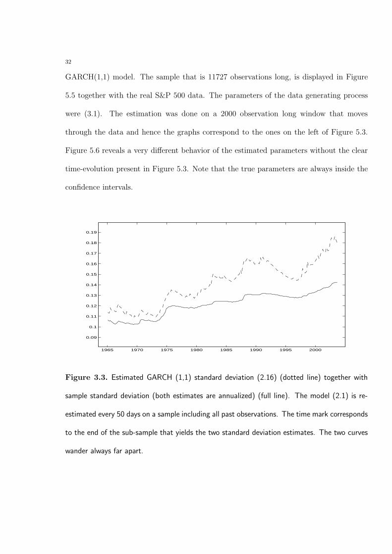
Figure 3.3. Estimated GARCH (1,1) standard deviation (2.16) (dotted line) together with

sample standard deviation (both estimates are annualized) (full line). The model (2.1) is re-

estimated every 50 days on a sample including all past observations. The time mark corresponds

to the end of the sub-sample that yields the two standard deviation estimates. The two curves

wander always far apart.

33

We end this section with a comparison between the point estimates of the GARCH(1,1)

unconditional variance and of the sample variance. Under the assumption of stationary

returns, the values of the parameters estimated on a growing sample containing all past

returns were used to produced the GARCH(1,1) unconditional sd (the broken line in Figure

3.3). The corresponding sample sd is depicted by the full line in the same figure. The

two curves wander wide apart suggesting that the GARCH(1,1) process estimated on an

increasing sample produces poor point estimates of the variance.

The evidence presented in this section indicates that the GARCH(1,1) process is not the

data generating process for the returns of the S&P 500 stock index between March 4, 1957

and October 9, 2003.

The significant changes of the value of the estimated parameters in Figure 5.3 suggests

that a more realistic working hypothesis is that of non-stationary data (in particular, the

unconditional variance could be time-varying). If this was the case, the GARCH(1,1) model

might turn out to, at least, provide good local stationary approximation to the process of

index returns. This issue is investigated in the next section.

3.2. Working hypothesis: The returns are non-stationary. The GARCH(1,1)

process is a local stationary approximation of the changing data. Working under

the assumption that unconditional features of the data might be also time-varying allows

us to provide a possible explanation for the poor unconditional variance point estimates

produces by the GARCH(1,1) model during the period May 16, 1995 to April 29, 2003

documented in section 2.1. The analysis in this section will also individuate all other

34

periods when the GARCH(1,1) model yielded point estimates of the unconditional variance

that were not in line with the sample unconditional variance and hence, failed to provide

a good local stationary approximation of the true data generating process of returns25.

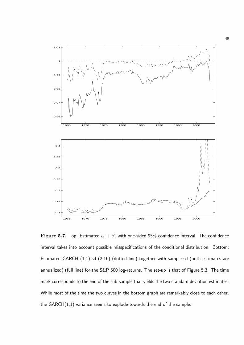
Figure 5.7 displays the estimated α1 + β1 under the assumption of non-stationary data.

The model (2.1) has been initially estimated on the first 2000 observations of the sample

in Figure 2.1 (bottom) corresponding roughly to the period 1957-1964, then re-estimated

every 50 observations on a sample containing 2000 past observations. The graph shows

that the IGARCH effect significantly26 affects the GARCH(1,1) models (estimated on a

sample that ends) during the period 1997-200327. This fact at its turn, is likely to cause

the explosion of the estimated unconditional variance of the GARCH(1,1) processes fitted

on samples that end during this period (see (2.18)).

To see that indeed this is the case, let us take look at the bottom graph of the same Figure

5.7 where the GARCH(1,1) unconditional sd (broken line) and the corresponding sample

sd (full line) are displayed. The GARCH(1,1) unconditional sd is obtained using (2.16)

from the values of the parameters estimated on a window of size 2000 moving through the

data and that are displayed in Figure 5.3. The graph shows a good agreement between

25A good local approximation model should fit reasonably well relatively short subsamples. In the sequel

we individuate only the periods when the GARCH(1,1) model does not provide an accurate description

of the unconditional variance. Of course, there could be that other stochastic features of the data are not

well-captured during the periods when the estimation of the unconditional variance is satisfactory.26The point estimate is close to 1 and, more importantly, 1 belongs to the 95% one-sided confidence

interval.

27During the interval 1994-1996, the value 1 is the upper bound of the confidence interval.

35

the two estimates at all times except during the period when the IGARCH effect becomes

strongly statistically significant, i.e. samples that end in the interval 1997-200328,29.

The bottom graph in Figure 5.7 together with the analysis in Section 2 show that the

GARCH(1,1) model fails to provide a local stationary approximation to the time series of

returns on the S&P 500 during significantly long periods.

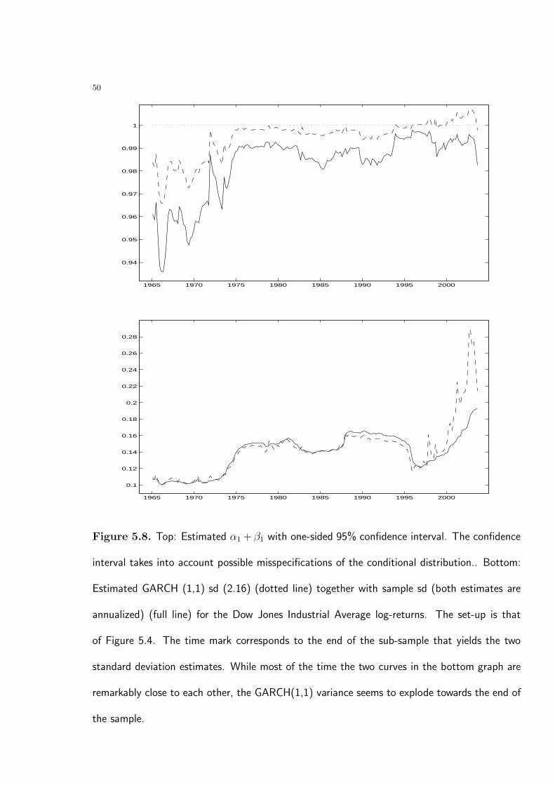
An analysis of the Dow Jones Industrial Average stock index produces similar findings.

The results are displayed in Figures 5.8.

An explanation for the strong IGARCH effect in the second half of the 90’s can be

the sharp change in the unconditional variance (see Mikosch and Starica [13]). There

it is proved, both theoretically and empirically, that sharp changes in the unconditional

variance can cause the IGARCH effect. Figure 3.4 displays non-parametric estimates of the

unconditional sd together with the 95% confidence intervals30 for the S&P 500 returns (top)

and the Dow Jones industrial index returns (bottom). The two graphs show a pronounced

28The analysis was also performed with smaller sample sizes of 1500, 1250 and 1000. As expected, the

confidence intervals in Figures 5.7 and 5.8 get wider and hence less meaningful. However, for every sample

sized mentioned, there is always a period between 1997 and 2003 where the unconditional variance of the

estimated model explodes. Estimation based on samples smaller than 1000 observations is infeasible as it

produces extremely unstable coefficients and renders problematic the use of any asymptotic result.29Contrast this finding with the statement on page 16 of the Advanced Information note: “Condition

α1 +β1 < 1 is necessary and sufficient for the first-order GARCH process to be weakly stationary, and the

estimated model (on the short S&P 500, n.n.) satisfies this condition.”30The method used to obtain the estimates is that of kernel smoothing in the framework of non-

parametric regression with non-random equi-distant design points. For more details on the performance

of this method on financial data see Mikosch and Starica [14].

36

increase of the volatility from around 5% in 1993-1994 to three times as much (around

15%) in the period 2000-2003.

1992 1994 1996 1998 2000 2002 20040

0.05

0.1

0.15

0.2

0.25

1992 1994 1996 1998 2000 2002 20040

0.05

0.1

0.15

0.2

0.25

Figure 3.4. Estimated unconditional standard deviation (annualized) with 95% confidence

intervals for the S&P 500 returns (top) and Dow Jones returns (bottom). The shaded areas

correspond to bear market periods.

3.3. The relevance of the GARCH(1,1) model for longer horizon forecasting of

volatility of index return series. As we have seen in section 3.1, the coefficients of the

37

GARCH(1,1) model change significantly through time. This phenomena raises naturally

the question about the relevance of the model for volatility forecasting over longer horizons.

This issue is investigated in the sequel by comparing the forecasting performance of a

GARCH(1,1) with that of a simple approach based on historical volatility. Both the S&P

500 data set and the Down Jones Industrial stock index returns are analyzed.

50 100 150 200 250

0.6

0.7

0.8

0.9

1

1.1

1.2

1.3

1.4

50 100 150 200 250

0.6

0.7

0.8

0.9

1

1.1

1.2

1.3

1.4

Figure 3.5. The ratio MSEGARCH/MSEBM . The MSE∗ are defined in (2.22). The

GARCH(1,1) model has been re-estimated on an increasing sample containing all past ob-

servations (left) and on a moving window of 2000 past observations (right). On the x-axis, p,

the forecast horizon.

The set-up is the one described in Section 2.3. A GARCH(1,1) model was estimated

on the first 2000 observations corresponding roughly to the period 1957-1964. Then the

model was re-estimated every 10 observations (every two business weeks) both on a sample

containing 2000 past observations and on a sample containing all past observations. Every

time the model was re-estimated, GARCH volatility forecast (see equation (2.18)) as well

38

as forecasts based on historical volatility (see equation (2.20)) were made for horizons from

1 day to 250 days ahead. The MSE for the two volatility forecasts were calculated using

(2.22) and the ratio MSEGARCH/MSEBM is displayed in Figure 3.5. While for shorter

(than 60 days ahead for locally estimated model and than 40 days ahead for a model

estimated on all past data) horizons, the GARCH(1,1) volatility forecast has a smaller

MSE, for longer forecasting horizons the historical volatility does significantly better.

50 100 150 200 250

0.6

0.7

0.8

0.9

1

1.1

1.2

1.3

1.4

50 100 150 200 250

0.6

0.7

0.8

0.9

1

1.1

1.2

1.3

1.4

Figure 3.6. The ratio MSEGARCH/MSEBM . The MSE∗ are defined in (2.22). The

GARCH(1,1) model has been re-estimated on an increasing sample containing all past ob-

servations (left) and on a moving window of 2000 past observations (right). On the x-axis, p,

the forecast horizon.

The results displayed in the graphs in Figure 3.5 seem to question the relevance of the

GARCH(1,1) dynamics for longer horizon volatility forecast of the S&P 500 return series.

The finding that the GARCH(1,1) dynamics provides a poor longer horizon forecasting

basis (when compared to a simple non-stationary approach centered on historical volatility)

39

documented for the S&P 500 return time series in Figure 3.5 was confirmed by similar

results for the Dow Jones Industrial stock index returns (see Figure 3.6).

1965 1970 1975 1980 1985 1990 1995 20000

0.05

0.1

0.15

0.2

0.25

0.3

0.35

0.4

0.45

1993 1994 1995 1996 1997 1998 1999 2000 2001 2002 20030.05

0.1

0.15

0.2

0.25

0.3

0.35

0.4

0.45

Figure 3.7. The realized 1-year ahead volatility (full line) together with the GARCH(1,1) fore-

casted volatility (dotted line) (top) for the S&P 500 data. The broken line in the bottom graph

is the historical volatility forecast based on the past 250 returns (all quantities are annualized).

Finally, Figure3.7 displays the realized 1-year ahead volatility, the GARCH(1,1) fore-

casted volatility and the historical volatility forecast based on the past 250 returns (all the

quantities are annualized). The graphs show a poor coincidence between the realized and

40

the forecasted GARCH(1,1) volatilities. Notably, the GARCH(1,1) forecast becomes espe-

cially volatile (even when compared with the forecast based on historical volatility) during

the period when the estimation of the model is significantly affected by the IGARCH effect,

i.e. the period that starts towards the end of 1997 and lasts to the end of the sample.

4. Conclusions

In this paper we investigated how truthful is the simple endogenous volatility dynamics

imposed by a GARCH(1,1) process to the evolution of returns of main financial indexes.

Our analysis concentrated first, on the series of S&P 500 returns between May 16, 1995 to

April 29, 200331 and was extended then to the longer series of S&P returns between March

4, 1957 and October 9, 2003.

The analysis of the shorter sample showed no (statistically significant) differences be-

tween a GARCH(1,1) modeling and a simple non-stationary, non-parametric regression

approach to next-day volatility forecasting.

We tested and rejected the hypothesis that a GARCH(1,1) process is the data generating

process for the series of returns on the S&P 500 stock index from March 4, 1957 to October

9, 2003. QML estimation of the parameters of a GARCH(1,1) model on a window that

moves through the data produced statistically different coefficients. Since the parameters

of the GARCH(1,1) model change significantly through time, it is not clear how the model

can be used for volatility forecasting over longer horizons.

31This series is featured in Section 3.2 of the Advanced Information note on the Bank of Sweden Prize

in Economic Sciences in Memory of Alfred Nobel.

41

We also evaluated the behavior of the GARCH(1,1) model as a local, stationary approx-

imation for the data. We have found that the IGARCH effect is not innocuous as it is

often claimed. In fact, it seems that during the periods when the IGARCH effect is sta-

tistically significant, the forecasting performance of the GARCH(1,1) model deteriorates

drastically at all horizons. Analyzing one of these periods, we found the MSE for longer

horizon GARCH(1,1) volatility forecasts to be up to more than four times bigger than a

simple forecast based on historical volatility.

In a forecasting comparison with a simple non-stationary approach centered on histori-

cal volatility, the finding that the GARCH(1,1) dynamics provides a poor longer horizon

forecasting basis was documented for the S&P 500 return time series as well as for the Dow

Jones Industrial Average index returns.

Acknowledgement: The constructive criticism of Holger Drees, Thomas Mikosch and

Richard Davis has benefited the paper, both in its conception and in its presentation.

42

5. Appendix: Big Figures

1 5000 9999−0.2

0

0.2

1 5000 9999−0.2

0

0.2

1 5000 9999−0.2

0

0.2

1 5000 9999−0.2

0

0.2

1 5000 9999−0.2

0

0.2

1 5000 9999−0.2

0

0.2

1 5000 9999−0.2

0

0.2

1 5000 9999−0.2

0

0.2

1 5000 9999−0.2

0

0.2

1 5000 9999−0.2

0

0.2

1 5000 9999−0.2

0

0.2

1 5000 9999−0.2

0

0.2

1 5000 9999−0.2

0

0.2

1 5000 9999−0.2

0

0.2

1 5000 9999−0.2

0

0.2

1 5000 9999−0.2

0

0.2

1 5000 9999−0.2

0

0.2

1 5000 9999−0.2

0

0.2

1 5000 9999−0.2

0

0.2

1 5000 9999−0.2

0

0.2

1 5000 9999−0.2

0

0.2

1 5000 9999−0.2

0

0.2

1 5000 9999−0.2

0

0.2

1 5000 9999−0.2

0

0.2

5000 10000−0.2

0

0.2

Figure 5.1. 24 randomly generated samples of length 11727 from the model (2.1) with pa-

rameters (2.2) (first 24 graphs). The S&P 500 returns from March 4, 1957 to October 9, 2003

(bottom-right). The aspect of the real data is different from that of the simulated samples.

43

References

[1] Andersen, T, Bollerslev, T. (1998) Answering the critics: Yes, ARCH models do provide goodvolatility forecasts. International Economic Review 39, 885–905.

[2] Berkes, I., Horvath, L. and Kokoszka, P. (2002) Probabilistic and statistical prop-erties of GARCH processes. To appear Fields Institute Communications. Available athttp://www.math.usu.edu/∼piotr.

[3] Bollerslev, T. (1986) Generalized autoregressive conditional heteroskedasticity. J. Econometrics31, 307–327.

[4] Bollerslev, T., Engle, R.F. and Nelson, D.B. (1994) GARCH models. In: Engle, R.F. andMcFadden, D.L. (Eds.) Handbook of Econometrics. Vol. 4, pp. 2961–3038. Elsevier, Amsterdam.

[5] Brockwell and Davis, R. (1987) Time Series: Theory and Methods. Second Edition. Springer,New York.

[6] Chu, C. and Marron, J. (1991) Comparison of two bandwidth selectors with dependent errors.Ann. Statist. 19, 1906–1918.

[7] French, K., Schwert, W. and Stambaugh, R. (1987) Expected stock returns and volatility. J.Financial Economics 19, 3–29.

[8] Gasser, T., Engel, J. and Seifert, B. (1993) Nonparametric function estimation. In: Computa-tional Statistics. Handbook of Statistics. Vol. 9, pp. 423–465. North-Holland, Amsterdam.

[9] Gijbels, I., Pope, A., and Wand, M. P. (1999) Understanding exponential smoothing via kernelregression. J. R. Statist. Soc. B, 51, 39–50.

[10] Gourieroux, C. (1997) ARCH Models and Financial Applications. Springer, New York.[11] Hsu, D.A., Miller, R., and Wichern, D. (1974) On the stable Paretian behavior of stock-market

prices. J. of American Statistical Association 69, 108–113.[12] Merton, R. (1980) On estimating the expected return on the market: an exploratory investigation.

J. Financial Economics 8, 323-361.[13] Mikosch, T. and Starica, C. (2004) Non-stationarities in financial time series, the long-

range dependence and IGARCH effects. Rev. Econom. Statist. To appear. Available underwww.math.ku.dk/∼mikosch.

[14] Mikosch, T. and Starica, C. (2003) Stock market risk-return inference. An unconditional non-parametric approach. Technical Report. Available under www.math.ku.dk/∼mikosch.

[15] Officer, R. (1976) The variability of the market factor of the New York Stock Exchange. J. Business46, 434–453.

[16] Straumann, D. and Mikosch, T. (2003) Quasi-MLE in heteroscedastic times series: a stochasticrecurrence equations approach. Technical Report. Available under www.math.ku.dk/∼mikosch.

[17] Taylor, S.J. (1986) Modelling Financial Time Series. Wiley, Chichester.[18] Wand, M.P. and Jones, M.C. (1995) Kernel Smoothing. Chapman and Hall, London.

44

1 5000 99990

0.005

0.01

1 5000 99990

0.005

0.01

1 5000 99990

0.005

0.01

1 5000 99990

0.005

0.01

1 5000 99990

0.005

0.01

1 5000 99990

0.005

0.01

1 5000 99990

0.005

0.01

1 5000 99990

0.005

0.01

1 5000 99990

0.005

0.01

1 5000 99990

0.005

0.01

1 5000 99990

0.005

0.01

1 5000 99990

0.005

0.01

1 5000 99990

0.005

0.01

1 5000 99990

0.005

0.01

1 5000 99990

0.005

0.01

1 5000 99990

0.005

0.01

1 5000 99990

0.005

0.01

1 5000 99990

0.005

0.01

1 5000 99990

0.005

0.01

1 5000 99990

0.005

0.01

1 5000 99990

0.005

0.01

1 5000 99990

0.005

0.01

1 5000 99990

0.005

0.01

1 5000 99990

0.005

0.01

1 5000 99990

0.005

0.01

Figure 5.2. The squares of 24 randomly generated samples of length 11727 from the model

(2.1) with parameters (2.2) (first 24 graphs). The squares of the S&P 500 returns from March

4, 1957 to October 9, 2003. The aspect of the real data is different from that of the simulated

samples.

45

1965 1970 1975 1980 1985 1990 1995 2000

0

0.5

1

1.5

2

2.5

3

3.5

4

4.5

5x 10

−6

1965 1970 1975 1980 1985 1990 1995 2000

0

0.5

1

1.5

2

2.5

3

3.5

4

4.5

5x 10

−6

1965 1970 1975 1980 1985 1990 1995 20000

0.05

0.1

0.15

0.2

1965 1970 1975 1980 1985 1990 1995 20000

0.05

0.1

0.15

0.2

1965 1970 1975 1980 1985 1990 1995 2000

0.75

0.8

0.85

0.9

0.95

1965 1970 1975 1980 1985 1990 1995 2000

0.75

0.8

0.85

0.9

0.95

Figure 5.3. Estimated coefficients of the model (2.1) for S&P 500 returns. The model

was initially estimated on the first 2000 observations of the sample in Figure 2.1 (bottom)

corresponding roughly to the period 1957-1964, then re-estimated every 50 observations on

a sample containing 2000 past observations (left column) and on a sample containing all the

past observations. The right column display the results of both estimations. The confidence

intervals take into account possible misspecifications of the conditional distribution (Gourieroux

[10], Berkes et al. [2], Straumann and Mikosch [16]). The dotted lines in the graphs on the left

are the parameters estimated on the whole sample. The graphs show pronounced instability of

the estimated values of the parameters.

46

1965 1970 1975 1980 1985 1990 1995 2000

0

0.5

1

1.5

2

2.5

3

3.5

4

4.5

5x 10

−6

1965 1970 1975 1980 1985 1990 1995 2000

0

0.5

1

1.5

2

2.5

3

3.5

4

4.5

5x 10

−6

1965 1970 1975 1980 1985 1990 1995 20000

0.05

0.1

0.15

0.2

1965 1970 1975 1980 1985 1990 1995 20000

0.05

0.1

0.15

0.2

1965 1970 1975 1980 1985 1990 1995 2000

0.75

0.8

0.85

0.9

0.95

1965 1970 1975 1980 1985 1990 1995 2000

0.75

0.8

0.85

0.9

0.95

Figure 5.4. Estimated coefficients of the model (2.1) for Dow Jones Industrial Average re-

turns. The model was initially estimated on the first 2000 observations of the sample in

Figure 2.1 (bottom) corresponding roughly to the period 1957-1964, then re-estimated every

50 observations on a sample containing 2000 past observations (left column) and on a sample

containing all the past observations. The right column display the results of both estimations.

The confidence intervals take into account possible misspecifications of the conditional distri-

bution (Gourieroux [10], Berkes et al. [2], Straumann and Mikosch [16]). The dotted lines in

the graphs on the left are the parameters estimated on the whole sample. The graphs show

pronounced instability of the estimated values of the parameters.

47

1960 1965 1970 1975 1980 1985 1990 1995 2000−0.09

−0.06

−0.03

0

0.03

0.06

1960 1965 1970 1975 1980 1985 1990 1995 2000−0.09

−0.06

−0.03

0

0.03

0.06

Figure 5.5. Top: Simulated S&P 500 returns (top). The sample has been obtained from

GARCH(1,1) process with parameters (3.1) estimated on the sample from March 4, 1957 to

October 9, 2003 (bottom).

48

1965 1970 1975 1980 1985 1990 1995 2000

0

1

2

3

4

5

x 10−6

1965 1970 1975 1980 1985 1990 1995 20000

0.05

0.1

0.15

0.2

1965 1970 1975 1980 1985 1990 1995 2000

0.7

0.75

0.8

0.85

0.9

0.95

1

Figure 5.6. Estimated coefficients of the model (2.1) on the simulated data in Figure 5.5.

The model has been initially estimated on the first 2000 observations of the simulated sample

corresponding roughly to the period 1957-1964, then re-estimated every 50 observations on a

sample containing 2000 past observations. The confidence intervals take into account possible

misspecifications of the conditional distribution (Gourieroux [10], Berkes et al. [2], Straumann

and Mikosch [16]). The true parameters are always inside the confidence bands.

49

1965 1970 1975 1980 1985 1990 1995 2000

0.96

0.97

0.98

0.99

1

1.01

1965 1970 1975 1980 1985 1990 1995 2000

0.1

0.15

0.2

0.25

0.3

0.35

0.4

Figure 5.7. Top: Estimated α1 + β1 with one-sided 95% confidence interval. The confidence

interval takes into account possible misspecifications of the conditional distribution. Bottom:

Estimated GARCH (1,1) sd (2.16) (dotted line) together with sample sd (both estimates are

annualized) (full line) for the S&P 500 log-returns. The set-up is that of Figure 5.3. The time

mark corresponds to the end of the sub-sample that yields the two standard deviation estimates.

While most of the time the two curves in the bottom graph are remarkably close to each other,

the GARCH(1,1) variance seems to explode towards the end of the sample.

50

1965 1970 1975 1980 1985 1990 1995 2000

0.94

0.95

0.96

0.97

0.98

0.99

1

1965 1970 1975 1980 1985 1990 1995 2000

0.1

0.12

0.14

0.16

0.18

0.2

0.22

0.24

0.26

0.28

Figure 5.8. Top: Estimated α1 + β1 with one-sided 95% confidence interval. The confidence

interval takes into account possible misspecifications of the conditional distribution.. Bottom:

Estimated GARCH (1,1) sd (2.16) (dotted line) together with sample sd (both estimates are

annualized) (full line) for the Dow Jones Industrial Average log-returns. The set-up is that

of Figure 5.4. The time mark corresponds to the end of the sub-sample that yields the two

standard deviation estimates. While most of the time the two curves in the bottom graph are

remarkably close to each other, the GARCH(1,1) variance seems to explode towards the end of

the sample.