5/19/01 1

Art as an Investment and the Underperformance of Masterpieces:

Evidence from 1875-2000

Jiangping Mei

Michael Moses1

April 2001

Abstract

This paper constructs a new data set of repeated sales of artworks and estimates an annual

index of art prices for the period 1875-2000. Contrary to earlier studies, we find art is

comparable to government bonds as an investment, though it significantly under-performs stocks

in the US. Art is also found to have lower volatility and lower correlation with other assets,

making it more attractive for portfolio diversification than discovered in earlier research. There

is strong evidence of underperformance of masterpieces, meaning expensive paintings tend to

under-perform the art market index. A further study reveals that the underperformance is

consistent with the presence of a winners curse due to excessive bidding. There is no

evidence, however, that the "law of one price" is violated in the New York art auction market.

(JEL G14, Z10)

1 Department of Finance and Department of Operations Management, Stern School of Business, New York University, 44 West 4th Street, New York, NY 10012-1126. We have benefited from helpful discussions with Will Goetzmann, Robert Solow and Larry White on art as an investment. We are grateful to Jennifer Bowe, Jin Hung and Loan Hong for able research assistance. We would also like to thank Mathew Gee of the Stern Computer Department for his tireless efforts in rationalizing our database. We also wish to thank John Ammer, John Campbell, Victor Ginsburgh, Robert Hodrick, Burton Malkiel, Tom Pugel and seminar participants at Temple University for helpful comments and John Campbell for his latent variable model algorithm. All errors are ours.

© Jianping Mei and Michael Moses.

5/19/01 2

Art as an Investment and the Underperformance of Masterpieces:

Evidence from 1875-2000

Abstract

This paper constructs a new data set of repeated sales of artworks and estimates an annual

index of art prices for the period 1875-2000. Contrary to earlier studies, we find art is

comparable to government bonds as an investment, though it significantly under-performs stocks

in the US. Art is also found to have lower volatility and lower correlation with other assets,

making it more attractive for portfolio diversification than discovered in earlier research. There

is strong evidence of underperformance of masterpieces, meaning expensive paintings tend to

under-perform the art market index. A further study reveals that the underperformance is

consistent with the presence of a winners curse due to excessive bidding. There is no

evidence, however, that the "law of one price" is violated in the New York art auction market.

(JEL G14, Z10)

5/19/01 3

Two major obstacles to analyze the art market are heterogeneity of artworks and

infrequency of trading. The present paper overcomes these problems by constructing a new

repeated-sales data set based on art price records at the New York Public Library as well as the

Watson Library at the Metropolitan Museum of Art. As a result, we have a significant increase

in the number of repeated sales comparing to an early studies by William J. Baumol (1986) and

William N. Goetzmann (1993).2 For the artworks included in the present study, we have 4,896

price pairs covering the period 1875-2000. With a larger data set, we are able to constructe an

annual art index as well as annual sub-indices for American, Old Master, Impressionist and

Modern paintings for various time periods. The annual indices are then used to address the

question of whether the risk-return characteristics of paintings compare favorably to those of

traditional financial assets, such as stocks and bonds.

The larger data set also permits us to test three propositions frequently advanced by art

dealers and economists. The first one states that art investors should buy only the top works of

established artists (masterpieces) or buy the most expensive artwork they can afford. The

empirical evidence on the return performance of masterpieces is mixed. James E. Pesando (1993)

presented strong evidence of underperformance while Goetzmann (1996) found no such

evidence. Our study will extend their analysis with a new testing procedure based on repeated

sales regression (RSR).

The second one states that art investors at auctions suffer from a winners curse. Under

the assumptions that all art bidders obtain unbiased estimates of a propertys value and that bids

are an increasing function of these estimates, then the high bidder tends to be the one with the

most optimistic estimates of the propertys value. Thus, unless this adverse selection problem is

accounted for, it will result in winning bids that produce below normal or negative profits. We

will study this proposition by using multiple repeated sales data. We will test one implication of

the winners curse: excess payment due to overbidding will lead to below average future returns.

2 Goetzmann (1993) uses price data recorded by Gerald Reitlinger (1961) and Enrique Mayer (1971-1987) to construct a decade art index based on paintings which sold two or more times, during the period 1715-1986. His data set contains 3,329 price pairs. Baumol (1986) uses a subset of the data recorded by Reitlinger (1961) to study the returns on paintings during the period 1652-1961. His data set contains 640 price pairs. Buelens and Ginsburgh (1993) re-exams Baumols work with different sample periods. Pesando (1993) uses data for repeat sales of modern prints which has 27,961 repeat sales. But his data only covers a short time span from 1977 to 1992.

5/19/01 4

One major obstacle for testing the winners curse in common value auctions is that the value of

the property is not observable. This paper partially circumvents this problem by assuming art

value is determined by its corresponding market index.3 As a result, given original purchase

price and the market index, we can compute a fair value for the property and measure excess

payment by taking the difference between purchase price and fair value. If there is a negative

relationship between excess payment and future returns, then there is evidence on the presence of

a winners curse. Numerous studies have examined common value auctions in which market

participants may be susceptible to winners curse. Due to the difficulties of observing the

common value and measuring future returns, the empirical literature on common value auctions

is long on experimental evidence and relatively short on field data.4 Our study will add to the

field literature by providing an empirical study of winners curse in art auction markets. We will

also try to link the underperformance of masterpieces to the winners curse. The third proposition states that prices realized for identical paintings at different

locations at the same time should be the same. Pesando (1993) compared prices of identical

prints sold at New York Sothebys and Christies and he found substantial evidence of violation

of the law of one price during the 1977-1992 period. While no art piece in our data has ever

been sold simultaneously in both auction houses, we will conduct a test of the law of one price

by examining the return differentials for artworks sold in the two houses over time. If there is

systematic pricing bias from one auction house to the other, then we should expect to see

systematic difference in returns for artworks sold at the two houses. We will examine the return

differentials with a RSR procedure that is different from Pesando (1993).

The remainder of the paper is organized as follows. Section I describes the art auction

data set and provides a discussion of sampling biases. Section II reviews the repeated sales

regression procedure used to estimate the index for painting prices and provides an asset-pricing

framework for estimating the systematic risk of paintings. Section III provides risk and return

3 Or more precisely, we assume that log art value is determined by its corresponding market index minus a constant with the constant reflecting a possible bidding bias. 4 For experimental evidence, see Bazerman and Samuelson (1983), Samuelson and Bazerman (1985), Weiner, Bazerman and Carroll (1987), and Kagel and Levin (1986). For field evidence on winners curse, see Dessauer (1981) on book publishing, Cassing and Douglas (1980) on baseball free agent, Capen, Clapp and Campbell (1971) and Mead, Moseidjord and Sorensen (1983) on oil drilling rights, and Thiel (1988) on bidding behavior in highway construction industry. Also see McAfee and McMillan (1987) for a comprehensive literature survey.

5/19/01 5

characteristics of the estimated art price index. Section IV presents evidence on the

underperformance of masterpieces. Section V investigates whether there is overbidding in the art

auction market and tries to link overbidding with the underperformance of masterpieces. Section

VI tests the hypothesis of the "law of one price" while Section VII concludes the paper.

I. Painting Data and Biases

Since individual works of art have yet to be securitized nor are there publicly traded art

funds, studying the increase in value of works of art from financial sources is not possible.

Gallery or direct-from-artists prices tend not to be reliable or easily obtainable. Repeat sale

auction prices however are reliable and publicly available (in catalogues) and can be used as the

basis for a data base for determining the change in value of art objects over various holding

periods and collecting categories.

We created such a database for the American market, principally New York. For the 2nd

half of the 20th Century we searched the catalogues for all American, 19th Century, Old Master,

Impressionist and Modern paintings sold at the main sales rooms of Sotheby's and Christies

(and their predecessor firms) from 1950 to 2000.5 If a painting had listed in its provenance a

prior public sale, at any auction house anywhere, we went back to that auction catalogue and

recorded the sale price. The New York Public Library as well as the Watson Library at the

Metropolitan Museum of Art were our major sources for this auction price history. Some

paintings had multiple resales over many years resulting in up to 6 resales for some works of art.

Each resale pair was considered a unique point in our database that now totals over five

thousand entries. Some of the original purchase dates went back to the 17th century. If the art

piece was sold overseas, we converted the sale price into US dollars using the long-term

exchange rate data provided by Global Financial Data. Our data has continuous observations

since 1871 and has numerous observations that allow us to develop an annual art index since

1875.

As well as analyzing our data as a totality we have also separated it into three popular

collecting categories. The first is American Paintings (American) principally created between

5 Our data does not include "bought-in" paintings that did not sell due to the fact that the bid was below reservation price. Our data for the year 2000 only includes sales before July.

5/19/01 6

1700 and 1950. The second is Impressionist and Modern Paintings (Impressionists) principally

created between the third quarters of the 19th and 20th century. The third is Old Master and 19th

century paintings (Old Masters) principally created after the 12th century and before the third

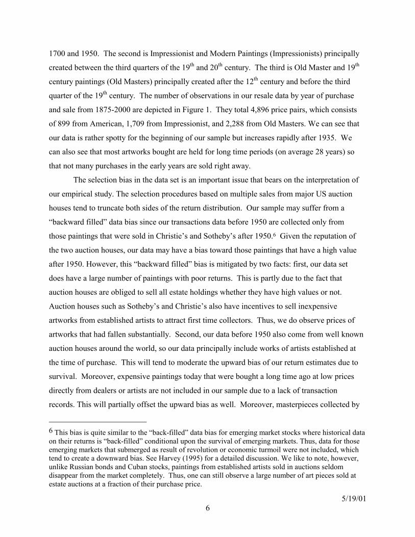
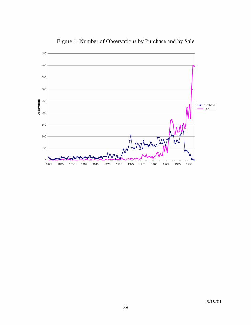
quarter of the 19th century. The number of observations in our resale data by year of purchase

and sale from 1875-2000 are depicted in Figure 1. They total 4,896 price pairs, which consists

of 899 from American, 1,709 from Impressionist, and 2,288 from Old Masters. We can see that

our data is rather spotty for the beginning of our sample but increases rapidly after 1935. We

can also see that most artworks bought are held for long time periods (on average 28 years) so

that not many purchases in the early years are sold right away.

The selection bias in the data set is an important issue that bears on the interpretation of

our empirical study. The selection procedures based on multiple sales from major US auction

houses tend to truncate both sides of the return distribution. Our sample may suffer from a

backward filled data bias since our transactions data before 1950 are collected only from

those paintings that were sold in Christies and Sothebys after 1950.6 Given the reputation of

the two auction houses, our data may have a bias toward those paintings that have a high value

after 1950. However, this backward filled bias is mitigated by two facts: first, our data set

does have a large number of paintings with poor returns. This is partly due to the fact that

auction houses are obliged to sell all estate holdings whether they have high values or not.

Auction houses such as Sothebys and Christies also have incentives to sell inexpensive

artworks from established artists to attract first time collectors. Thus, we do observe prices of

artworks that had fallen substantially. Second, our data before 1950 also come from well known

auction houses around the world, so our data principally include works of artists established at

the time of purchase. This will tend to moderate the upward bias of our return estimates due to

survival. Moreover, expensive paintings today that were bought a long time ago at low prices

directly from dealers or artists are not included in our sample due to a lack of transaction

records. This will partially offset the upward bias as well. Moreover, masterpieces collected by

6 This bias is quite similar to the back-filled data bias for emerging market stocks where historical data on their returns is back-filled conditional upon the survival of emerging markets. Thus, data for those emerging markets that submerged as result of revolution or economic turmoil were not included, which tend to create a downward bias. See Harvey (1995) for a detailed discussion. We like to note, however, unlike Russian bonds and Cuban stocks, paintings from established artists sold in auctions seldom disappear from the market completely. Thus, one can still observe a large number of art pieces sold at estate auctions at a fraction of their purchase price.

5/19/01 7

museums through donation rather than auction sales are also excluded from the sample, further

offsetting the upward bias.

In addition to these selection biases, Orley Ashenfelter, Kathryn Graddy, and Margaret

Stevens (2001) pointed out that not all items that are put up for sale at auctions are sold because

some biddings may not reach reservation prices. Goetzmann (1993) also argues that the decision

by an owner to sell a work of art (and consequently the occurrence of a repeat sale in the sample)

could be conditional upon whether or not the value has increased. These would also tend to bias

the estimated return upward.7 Because of these biases, the mean annual return to art investment

provided by repeated-sale data should be regarded as approximate, or as an upper bound on the

average return obtained by investors over the period. The return could be further reduced by

transaction costs. We like to note, however, that return estimates for financial assets, to some

extent, also could suffer from the same biases, such as lack of market liquidity, transaction costs

and survival.

II. Methodology for Estimating the Art Index and Asset Pricing

The repeat-sales regression (RSR) uses the purchase and sale price of individual

properties to estimate the fluctuations in value of an average or representative asset over a

particular time period. Robert C. Anderson (1974), Goetzmann (1993), and Pesando (1993)

apply it to the art market. The benefit of using the RSR is that the resulting index is based upon

price relatives of the same painting that controls for the differing quality of assets. Thus, it does

not suffer from arbitrary specifications of a hedonic model. The drawback is that the index is

constructed from multiple sales, which is a subset of the available transactions. Olivier Chanel,

Louis-Andre Gerard-Varet, and Victor Ginsburgh (1996) provided a detailed discussion on the

weakness of RSR model.

7 Goetzmann (1993, 1996) also argues that auction transactions may not adequately reflect an important element of risk for the art investor: stylistic risk. In other words, the future sales price will depend upon the number of people who wish to buy the work of art when it is put up for sale. Since the repeat-sales data principally reflect auction transactions, they necessarily focus upon artworks that have a broad demand to attract a large number of competitive bidders. Thus, the repeat-sales records will fail to capture the price fluctuations of paintings that are not broadly in demand. The stylistic risk is similar in many respects to the liquidity risk in financial markets, where prices of assets are affected not only by fundamental values but also by market liquidity.

5/19/01 8

We begin by assuming that the continuously compounded return for a certain asset i in

period t, ri,t, may be represented by µt, the continuously compounded return of a price index of

art, and an error term:

ri,t = µt + ηit (1)

where µt, may be thought of as the average return in period t of paintings in the portfolio. We

will use sales data about individual paintings to estimate the index µµµµ over some interval t = 1...

T. Here, µµµµ is a T-dimensional vector whose individual elements are µt. The observed data

consist of purchase and sales price pairs, Pi,b, and Pi,s, of the individual paintings comprising the

index, as well as the dates of purchase and sale, which we will designate with bi, and si. Thus,

the logged price relative for asset i, held between its purchase date bi and its sales date, si, may

be expressed as

∑ ∑

∑

+= +=

+=

+=

=

=

i

i

i

i

i

i

s

bt

s

bttit

s

btti

bi

sii r

PP

r

1 1,

1,

,

,ln

ηµ (2)

Let r represent the N-dimensional vector of logged price relatives for N repeated sales

observations. Goetzmann (1992) shows that a generalized least-squares regression of the form

( ) r''ˆ 111 −−−= ΩΧΧΩΧµ (3) provides the maximum-likelihood estimate of µµµµ, where X is an NxT matrix, which has a row of

dummy variables for each asset in the sample and a column for each holding interval. Ω is a

weighting matrix, whose weights could be set as the times between sales as in Goetzmann

(1993) or could be based on error estimates from a three-stage-stage estimation procedure used

by Karl E. Case and Robert J. Shiller (1987).8

8 The RSR is known to introduce certain biases in the estimated series. The most serious of these are a spurious negative autocorrelation in the estimated return series. This bias is potentially severe when the number of assets in the sample is low, and it is strongest at the beginning of the estimated series, when the sample is small. Goetzmann (1992) propose a two-stage Bayesian regression to mitigate the negative autocorrelation of the series over the early periods. The Bayesian formulation imposes an additional restriction that the return series µµµµ, is distributed normally and is independently and identically-

5/19/01 9

To calculate the standard errors associated with estimation error for any statistic, such as

the mean return of the art index, we first let µ and V represent the whole set of return parameters

and their variance-covariance matrix respectively. Next, we write any statistic, such as the mean

return, as a function f(µ) of the parameter vector µ. The standard error for the statistic is then

estimated as the square root of fµVfµ, where fµ is the gradient of the statistic with respect to the

parameters µ. This is often called the δ method in econometrics.

To estimate the systematic risk of art as investment, we follow John Y. Campbell (1987)

by assuming that capital markets are perfectly competitive and frictionless, with investors

believing that asset returns are generated by the following K-factor model:

[ ] ∑=

++++ ++=K

ktitkiktitti feEe

11,1,1,1, ξβ (4)

Here ei,t+1 is the excess return on asset i held from time t to time t+1, and represents the

difference between return on asset i and the US treasury bill rate. Et[ei,t+1] is the expected

excess return on asset i, conditional on information known to market participants at the end of

time period t. We assume that Et[fk,t+1] = 0 and that Et[ξi,t+1] = 0. The conditional expected

excess return is allowed to vary through time in the current model but the beta coefficients are

assumed to be constant. This ability of Et[ei,t+1] to vary through time is absent in prior art

studies. Equilibrium asset pricing suggests the following linear pricing relationship:

[ ] ∑==

+

K

kktiktit eE

1,1, λβ (5)

where λkt is the "market price of risk" for the k'th factor at time t.9

distributed. The effect on the estimate is dramatic for the early period when data are scarce, and minimal for the period when data are plentiful. The form of the- Bayesian estimator is:

( ) rJT

IBayes1

11 '1' −

−− ΩΧ

−+ΧΩΧ= κµ

Goetzmann and Peng (2001) also proposed an alternative repeated sales estimate that is unbiased and based on arithmetic average of returns. 9Equation (2) states that the conditional expected rate of return should be a linear function of factor risk premiums, with the coefficients equal to the betas of each asset. This type of linear pricing relationship can be generated by a number of inter-temporal asset pricing models, under either a no arbitrage opportunity condition or through a general equilibrium framework. See for example, Ross (1976).

5/19/01 10

Now suppose that the information set at time t consists of a vector of L forecasting

variables Xnt, n=1...L (where X1t is a constant), and that conditional expectations are a linear

function of these variables. Then we can write λkt as

∑=

=L

1n,ntkn,kt Χθλ (6)

and plug it into equation (5) and collect terms, it becomes,

[ ] ∑∑== =

+ Χ∑ =Χ=L

nntin

K

k

L

nntkniktit eE

11 11, αθβ (7)

Equations (5) and (7) combined are sometimes called a multi-factor "latent-variable" model.10

The model implies that expected excess returns are time-varying and can be predicted by the

forecasting variables in the information set. From equation (7), we can see that the model puts

some restrictions on the coefficients of αij:

∑=

=K

1k,kjikij θβα (8)

Here, βik and θkj are free parameters. We will use the regression system in equation (7) to

see to what extent the forecasting variables, X, predict excess returns in art investment and to see

how closely the risk premium on art move with those on other assets. In general, we do not wish

to assume that we have included all of the relevant variables that carry information about factor

premiums. Fortunately, the methods described above are robust to omitted information.11 The

regression system of equation (7) given the restriction in equation (8) can be estimated and tested

using Lars Peter Hansen's (1982) Generalized Method of Moments (GMM).

Our methodology here has several distinctive advantages over previous studies. First, it

allows for time-varying risk premiums. Second, the GMM estimation procedure adjusts for

heteroskedasticity in the error terms and permits contemporaneous correlation among the error

10For more details on this model, see Campbell (1987) and Ferson and Harvey (1990). 11By taking conditional expectations of equation (2), it is straightforward to show that the pricing restrictions hold in the same form when a subset of the relevant information is used. A more detailed elaboration of this robustness issue is discussed in Campbell (1987).

5/19/01 11

terms across assets. A more detailed discussion of this estimation procedure is provided in the

Appendix.

In computing ri,t+1, we use return indices from six different asset class: the Art index,

Standard and Poor's 500 Total Return Index, the Dow Jones Industrial Total Return Index, the

US Government Bonds Total Return Index, the US Corporate Bond Total Return Index, and the

United States Treasury Bills Total Return Index.12 With the exception of the art index, the

sources of these data are from Federal Reserve Board and Global Financial Data (5th edition),

which has derived its data from historical data on prices and yields collected by Standard and

Poors, the Cowles Commission and G. William Schwert (1988).

III. Risk and Return Characteristics of the Art Price Index

Figure 2 provides a graphic plot of the art index over the 1875-1999 period with the base

year index set to be 100. The index is estimated with 4,896 pairs of repeated sale prices. Our

reported art index is based on the three-stage-least-square procedure proposed by Case and

Shiller (1987).13 The Adjusted R-squares for the estimation is 0.64, suggesting the art index

explains 64% of the variance of sample return variation. The F-statistic equals 120.62 with a

significance level equal to 0.000, indicating the index is a highly significant common return

component of our art portfolios. Due to a smaller number of observations, the three sub-indices,

American, Impressionist, and Old Masters, were estimated only for the 1942-1999, 1942-1999,

and 1900-1999 periods respectively. The mean annual returns for the three sub-indices were

12 To estimate equation (7), we also use the following forecasting variables Xnt which are known to the market at time t. They include a constant term, the yield on US treasury bills, the dividend yield on Standard and Poor's 500 index, the dividend payout ratio on the Standard and Poor's 500 index, the spread between the yields on Moody's Baa Corporate Bond and US government bonds, and the spread between the yields on US government bonds and US treasury bills. The dividend yield and dividend payout variables capture information on expectations about future cash flows and required returns in the stock market. The two bond spread variables tells us the default premium and the slope of the term structure of interest rates. These variables have been used by Campbell (1987), Fama and French (1988, 1989), Ferson and Harvey (1991), and Lamont (1998), among others. 13 We use the Case and Shiller (1987) procedure because it allows us to adjust for a downward bias in annual returns estimation due the log price transformation (see Goetzmann (1992)). We have also estimated the art index using GLS and the two-stage Baysian estimation proposed by Goetzmann (1992). The correlation between the Case and Shiller (1987) procedure and the other two procedures are 0.956 and 0.906, suggesting that the results are quite robust. We have also discovered that the two-stage Baysian estimates tend to have smaller estimation errors though they may be biased.

5/19/01 12

6.3%, 6.2% and 5.4% respectively. Thus, the performance of American paintings was essentially

the same as that of Impressionist paintings during the 1942-1999 period, despite the fact that

some Impressionist paintings fetched sky-high prices in the 1980s. The figure shows a sharp rise

in prices in the 1980s with the art index peaked at 1522 followed by an 18.7% drop in 1991.

Thus, performance is much affected by the bear market in art of last ten years. If we exclude the

last ten years, the mean returns would be 7.4%, 7.7% and 5.8% respectively. While the boom

and bust was well documented in the art market, the price indices allows us to estimate the

precise time and magnitude of the price change. Our indices have also identified major price

drops during the 1974-75 oil crisis and 1929-1934 depression.

Table 1 provides summary statistics on the behavior of returns for each of our six asset

classes. For each variable, we report the mean, standard deviation, and its correlation with other

assets. We also report the standard deviation of art return estimates due to estimation error using

the δ method. We can see that our estimates are fairly accurate. The standard error for the mean

return estimate was 1.1% for the 1875-2000 period. It was only 0.2% for the 1950-2000 period

due to more observations in the later period. Table 1 reveals that art had a higher return relative

to government bonds and treasury bills. More specifically, during the period of 1875-1999, the

mean annual returns on art was 5.6%, higher than the 4% and 4.3% mean return obtained by

government bonds and treasury bills respectively.14 However, art under-performed corporate

bonds and stocks. Corporate bonds derived a 5.7% annual return while the S&P 500 and the Dow

Industrial gained 11.1% and 12.4% annual return respectively. Our results are quite similar for

the 1900-1999 sample period. The art index, however, under-performed all other assets except

treasury bills in the last half of twentieth century. But interestingly, the volatility of art market

price index has dropped to 9.3%, making art no more risky than government and corporate

bonds.15

These results contrast with those of Goetzmann (1993) using securities data from UK. He

found that art significantly out-performed both stocks and bonds in UK during 1850-1986 and

1900-1986 sample periods.16 For the longer sample period of 1716-1986, his art index actually

14 We did not include the year 2000, since our data only has sales from the first half of the year. 15 The dramatic reduction in art index volatility should be expected, since the number of artworks in our art index portfolio increased rapidly after 1940 due to sample selection. 16 It is worth noting that, while both Goetzmanns (1993) and our data include artworks sold internationally, Goetzmanns data are concentrated in UK sales before 1960 and ours are skewed towards

5/19/01 13

out-performed stocks but under-performed bonds in UK. The differences in art performance

results are partly due to difference in sample selection and partly due to the fact that his sample

ended in 1986, prior to the collapse in art prices. In comparison to his findings, our art index

shown in Table 1 has much less volatility and much lower correlation with other asset class. As

a result, a diversified portfolio of artworks may play a somewhat more important role in portfolio

diversification than discovered in earlier research. Our results are also different from Pesando

(1993) using modern prints sold in US and Europe. He found modern prints under-performed

both stocks and bonds during 1977-1992 sample period, but print returns could be less volatile

than stock and bonds.17

In Table 2, we report the estimates of the restricted version of our asset pricing model (4)

with restriction (8) imposed. The estimation method used is the GMM procedure of Hansen,

using the forecasting variables given in footnote 12. We estimate our model under the

assumption that there is only one "priced" systematic factor, f1,t+1, in the economy (K=1). With

beta normalized to be 1 for the S&P 500 index, we observe that the beta for art is higher than the

one on bonds. The beta on art was 0.674 during the sample period and it was highly significant

with a t-statistic of 3.035. This is consistent with Goetzmann (1993) who found that art prices

are affected by a wealth effect from the stock market. The betas on government and corporate

bonds were 0.084 and 0.217 respectively. The chi-square test indicates that a one-factor model is

rejected by the data at a 5% significance level but a two-factor model is not rejected.18

IV. Do Masterpieces Under-perform?

A common advice given to their clients by art dealers is to buy the most expensive

artworks they can afford. This presumes that the masterpieces of well known artists will

auction sales in the US. While our result on art return characteristics is similar to Goetzmann (1996), he did not use a RSR estimation approach in his 1996 paper. 17 Our average return results are similar to those of Buelens and Ginsburgh (1993) from the 1870-1913 period. But they did not make comparison to the returns of financial assets. They also cover a different sample period based on the Reitlinger (1961) data. 18 It is well known in the finance literature that a one-factor CAPM model is often rejected by data. We still report the estimates of the one factor model because it is quite interesting to know the beta of the art return index. We have also estimated a "two factor" model with a stock market factor and a bond factor. Our results indicate that art is still more sensitive than corporate bonds to the market factor, while

5/19/01 14

outperform the market. In other words, masterpieces might have a higher expected return than

middle-level and lower-level works of art. Contrary to this popular belief, Pesando (1993)

discovered that masterpieces actually tend to under perform the market. His discovery was based

on repeated sales of modern prints from 1977-1992. Since Pesandos data only cover prints that

tend to have much lower value compared to 19th century old masters and impressionists

paintings, one may wonder if this underperformance exists for truly expensive artworks.

Moreover, Goetzmann (1996) found no evidence of underperformance of masterpieces. Using

repeated sales data covering American, 19th Century Old Master, Impressionist and Modern

paintings, this paper will further examine the performance of masterpieces. We will follow

Pesando by using the market price to identify the masterpieces (i.e, expensive paintings are

masterpieces). In the first examination, we use prices for all artworks sold between 1875 and

2000. We apply the same repeated sales regression approach used in the section above by adding

an additional term in the regression,

( ) ∑∑+=+=

+Ρ⋅−+=i

i

i

i

s

btitbiii

s

btti bsr

1,

1ln εγµ (9)

where γ is the elasticity of art returns with respect to log price of the property and (si-bi) is the

holding period. Here γ gives the expected percentage changes in annualized returns as a result of

a 1% change in art purchase prices. For the three subcategories, we also repeat the same

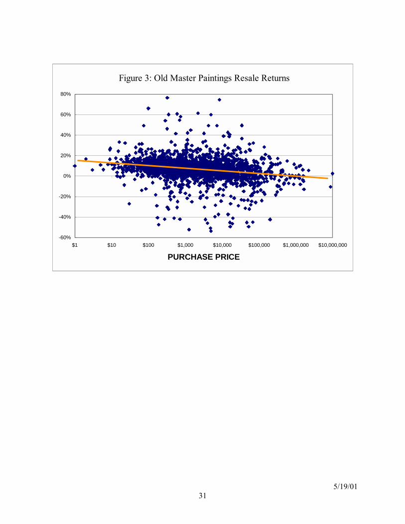
estimation procedure. In the second exercise, we use prices deflated by the US CPI index, since

the nominal value of art may change due to inflation. The results are reported in Table 3 while

Figure 3 provide a simple plot of art returns and purchase prices for Old Masters paintings. Our

results are uniform across all categories that masterpieces significantly under-performed their

respective art market indices. Our γ estimate on the American artworks indicates that a 10%

increase in purchase price is expected to lower future annual returns by 0.1%. Moreover, our

results are robust to whether nominal prices or real prices are used in the regressions. Thus, our

study seems to suggest that art investors should buy less expensive artworks from auction

houses.

corporate bonds appear to be more sensitive than art and stocks to the bond factor. The results are available upon request.

5/19/01 15

The underperformance of masterpieces is similar to the small firm effect documented

by K.C. Chan and Nai-Fu Chen (1988) and many others in their study of the capital asset pricing

model. These authors discover that small firms with lower market capitalization tend to achieve

excess returns not justified by their risk based on single factor market models. Recent studies by

Eugene Fama and Kenneth French (1996), however, suggest that firm size could be a proxy for

exposure to systematic risk factors.19 While it may be possible to argue that masterpieces are

less risky, we will show in the following section that the underperformance of masterpieces

could be explained by the presence of the winners curse in art auctions.

V: Are Masterpieces Cursed by Overbidding?

Richard H. Thaler (1988) provided a comprehensive literature review on winners curse.

It is a concept that originated in the study of bidding behavior by oil companies in their

purchasing of drilling rights to land parcels. Assuming people purchase art as investment, we

can describe an art auction as a common value auction,20 where the value of property is assumed

to be worth the same amount to all bidders. Further, we suppose that art value is hard to estimate

so that each bidder can only obtain an estimate of the value. Assume that the estimates are

unbiased, so the mean of the estimates is equal to the common value of the artwork. Given the

difficulty of estimating art value, these estimates from different bidders are likely to vary

substantially, some too high and some too low. Even if the bidder bid somewhat less than his or

her estimate, those bidders who have high estimates will tend to bid more than those who

guessed lower. Indeed, it may occur that the bidder who wins the auction will be the one whose

estimate is the highest. If this happens, the winner of the auction is likely to be a loser. The

winner can be said to be "cursed" in the sense that the purchased piece will receive less than the

expected return or perform poorly comparing to other artworks for which the purchase prices are

closer to their values. The higher the winning price in relation to value, the lower the future

returns. In other words, the higher the excess payment over value, the lower the expected returns

19 Alternatively, one may argue that many people purchase art for their own pleasure and more expensive paintings have larger private consumption values. Thus, the negative returns could indicate a higher private consumption value offset by a lower monetary payoff in an efficient art market. 20 For art and wine auctions, see Ashenfelter (1989).

5/19/01 16

for the future holding period. Notice that the curse can still apply even if the winning bidder

makes a positive return, as long as the return is less than expected at the time the bid was made.

This paper constructs a new test of winners curse by using multiple sales data from art

auctions. The repeated sales data allows us to observe the purchase price by a previous owner,

the purchase price paid by the bidder and her sale price after the holding period. One main

difficulty of conducting such a test is that the true value is unobservable so it is impossible for

researchers to gain an accurate measure of excess payment. We get around this difficulty by

assuming that art value is determined by its corresponding market index. (Or more generally, we

assume that log art value is determined by its corresponding log market index minus a constant with the

constant reflecting a possible average bidding bias. One can see the constant term cancels out in our

computation of excess payment.) In other words, we assume that art value increase with its market

index at the same rate after its previous purchase. As a result, given the first purchase price and

the market index, we can compute a fair value for the property at the second purchase and

measure excess payment by studying the difference between second purchase price and fair

value. If there is a negative relationship between excess payment and future returns, then there

is evidence on the presence of a winners curse. Using 494 sets of multiple sales data spanning

from 1875 to 2000, we run two regressions:

eri = θ0 + θ1epi + ζi, (10)

and

eri = θ0 + θ1epi +θ2ln(Pi,b’) + ζi, (11)

where eri is excess annual return over the market index for the holding period on property i after

the bidder paid Pi,b at the second sale. epi is log excess payment, which is defined as log

(Pi,b/Pi,b)/(Ii,b/Ii,b), where Pi,b/Pi,b is the appreciation of the property during the previous holding

period and Ii,b/Ii,b is the index appreciation during the corresponding period. ti is the length of

the second holding period. The intuition behind the excess payment is that the relative

appreciation of the property over that of the corresponding art index during the same period

provides a measure of excess payment on the property that may lead to lower returns in the

future. Here, we use equation (10) to measure the direct relationship between excess payment

and future returns and we use equation (11) to control for the masterpieces, so that we can rule

5/19/01 17

out the possibility that the low future returns are due to underperformance by masterpieces and

not excess payment resulted from excessive bidding. The results are reported in Table 4 and

Figure 4.

Our results suggest that, with the only exception of American art, there is a significant

negative relationship between excess payment and future excess returns. Our θ1 estimate on the

Impressionists indicates that a 10% increase in excess payment is expected to lower future

annual excess returns by 0.16% from its mean. As we can see clearly from Figure 4, most

bidders have made excess payment (epi>0), i.e., paid more than the market appreciation. While

the market index might be subject to estimation error, there is clear evidence that future excess

returns are negatively related to excess payments, though not all excessive biddings resulted in

negative excess returns.21 This negative relationship between excess payments and future excess

returns indicate that there is little persistence in art returns. Past winners (which fetched high sale

prices at auctions and became masterpieces) tend to under perform the art market index in the

future. In other words, there is regression to the mean in the art market.

Due to the fact that the true value of art is not observable, we cannot make a statement

whether there is systematic overbidding in the auction market at all times. As a matter of fact, as

long as the systematic overbidding is constant over time in log value, it cancels out in the return

computation and thus do not affect our results. What our results do show, however, is the

presence of overbidding at the cross-sectional level (individual art piece) that are negatively

related to future investment returns. In many respects, our results are similar to those found in

Werner F. M. De Bondt and Richard Thaler (1989) about the stock market. They discovered a

mean reversion in stock returns. Those stocks that outperformed the stock market (winners) in

the past tend to under perform in the future while those that under performed (losers) tend to

outperform in the future. De Bondt and Thaler attributed this mean reversion to investor over-

reaction. Our results confirm similar mean reversion is present in the art market as well, possibly

due to the existence of a weaker form of the winners curse, that there are suboptimal

investment behaviors by some art buyers who engaged in excessive bidding.

21 We have also estimated equation (11) by eliminating the outliers with future excess returns greater than 50% or lower than 50%. Our results remain unchanged. We confirmed our results with data from Impressionists and Old Masters, which had 99 and 288 observations, respectively. The tests for American paintings were not conclusive due to a lack of observations. These results are available upon request.

5/19/01 18

Table 4 further shows that the excess payment term remains significant even if we include

the log price variable for masterpieces. Our results indicate that, after controlling for the

presence of excess payment, masterpieces did not significantly under perform (especially for the

1875-1975 period). Thus, it is not high prices per se that contributed to lower average returns

but excess payments.22 In other words, masterpieces were only cursed if their buyers paid

excessively high prices above the market. What is also interesting is that even after a century of

data from 1875-1975, which showed a significant negative relationship between excess payment

and future excess returns, art buyers after 1975 still demonstrated a tendency for over-bidding,

which resulted in lower average returns.23 These results are reported in the two bottom panels of

Table 4. We have also broken the sample using other years, such as 1950 and 1960 rather than

1975, and the results remain unchanged. Thus, the puzzle is why art investors would

consistently ignore this negative relationship?24

One rational explanation is that the mean reversion found in the paper does not allow a

dealer to trade profitably by buying low and selling high. To do so, she would have to inventory

such paintings, which she would have to put up substantial capital. In addition, she faces 10%

buyers commission and 6% sellers commission for dealers (10% for others). Given the price

volatility, the arbitrage is hardly risk-free. Moreover, the data and technology for estimating the

art market index may not be available to the average dealer so that she may not be able to

estimate excess payment and be aware of the winners curse in the art auctions.

Another explanation for the mean reversion is that art prices are also determined by

private consumption values of artworks. The lack of a well-developed rental market suggests

that the owner's personal enjoyment is an important component of the unobserved yield. One

could argue that the purpose of the auction is to allocate the item to the person who likes it best.

Thus if there is a buyer (or perhaps two, to bid up the price) who is particularly fond of a

particular item, than the value should go up when she first sees it. The dividend stream

22As a robustness check, we also estimated equation (12) using excess payment, (Pi,b/Pi,b)-(Ii,b/Ii,b), and annualized log excess payment as [log (Pi,b/Pi,b)/(Ii,b/Ii,b)]/(b-b). Our results remain unchanged. The results are available upon request. 23 Even after controlling for excess payment, the underperformance of masterpieces remains significant for properties bought after 1975. This may reflect a nonlinear over payment effect as a result of the feverish bidding on impressionists during the 1980s. 24 In some instances, the log excess payments exceeded 8, suggesting some artworks were bought at such high prices that the return to the previous owner exceeded 500 times the art market index return!

5/19/01 19

(enjoyment) is higher as long as this buyer lives (or can afford to own it), but will likely be lower

again if her heir (or she) decides to sell it. This ought to produce the mean reversion in relative

price changes.25 One could also easily explain away the under performance of masterpieces by

arguing that the lower performance is compensated by a large unobserved aesthetic consumption

yield produced by the masterpieces.

VI: Tests of “Law of One Price”

Pesando (1993) compared prices of identical prints sold in different markets, and he

found substantial evidence of violation of law of one price during the 1977-1992 period. He

found that prices for prints sold at Sothebys consistently exceed prices of those sold at

Christies. This is puzzling, since one would expect, in the absence of transaction costs, the law

of one price would dictate that no significant price difference should exist for identical prints of

the same artist. Ashenfelter (1989) also discussed the violation of law of one price on wine

auctions around the world.

This paper provides an alternative test of the law of one price using the repeated sales

data for original paintings from Christies and Sothebys. Our null hypothesis is that there is no

difference between prices realized at Sothebys and prices realized at Christies so that the

returns realized from both auction houses are equal. To test the above hypothesis, we include an

annualized return dummy for Sothebys in the following repeated sales regression:

( ) ∑∑+=+=

+⋅−+=i

i

i

i

s

btitiii

s

btti Dbsr

11ερµ (12)

where Di is a dummy variable for Sothebys based sales and ρ measures the excess annual return

achieved by Sothebys over Christies due to possible difference in auction prices. Equation (12)

is estimated the same way as equation (2) by adding a dummy variable column to the matrix X in

equation (3). The results are presented in Table 5. Contrary to what was found in Pesando

(1993), here we have no evidence to reject the hypothesis that returns for properties sold at

Sothebys are different from those sold at Christies. While the estimates indicate a 0.8% return

25 We are grateful to John Ammer for providing this alternative explanation.

5/19/01 20

difference between the two auction houses for American paintings, the difference was not

statistically significant. Our results are quite robust with respect to different time periods for

various collection categories. Thus, sellers should be indifferent from selling through either

Sothebys or Christies since they essentially obtain the same returns (sale prices).

VII. Conclusions

This paper constructs a new data set of repeated sales of art paintings and estimates an

annual index of art prices for the period 1875-2000. Our data set has more repeated sales data

than previous studies and is also broken down by three popular collecting categories.

Based on this new data set, our study made the following discoveries: First, contrary to some

earlier studies, we find art is comparable to government bonds as a long-term investment, though

it significantly under-performs stocks. Our art index also has less volatility and much lower

correlation with other asset classes as found in previous studies. As a result, a diversified

portfolio of artworks can play a somewhat more important role in portfolio diversification.

Second, our study finds strong evidence of underperformance of masterpieces as in Pesando

(1993), which means expensive paintings tend to under perform the art market index. By

measuring excess return on art investment on multiple sales, we have found that the

underperformance of masterpieces is actually a symptom of a weak form of winners curse.

The curse tends to punish those bidders who pay excessive amount relative to "fair value" with

lower future returns. This curse appears to be more pronounced for impressionist paintings that

went through a boom and bust cycle in the last twenty years.

Thirdly, there is no evidence that the "law of one price" is violated in the New York art

auction market. More specifically, prices realized at Sothebys are found to be not significantly

different from those at Christies over the sample period as indicated by essentially the same

rates of returns obtained at the two auction houses.

Our results on the return-risk characteristics of artworks and the correlations between art

and financial assets have implications for long-term investors. If the art market volatility

remains stable at the level of 1950-1999, then our estimate of the risk of the art index suggests

that the total value of a large collection diversified broadly across different styles is likely to be

no more risky than a corporate bond portfolio. The low correlations with other asset classes also

5/19/01 21

make art a possible choice for portfolio diversification. Contrary to established industry wisdom,

our results on the performance of masterpieces suggest that investors should not be obsessive

with masterpieces and they need to guard against overbidding that exceeds overall market

appreciation. We like to note, however, our results may only serve as a benchmark for those

artworks bought at major auction houses. Our return estimates could be biased due to sample

selection. In addition, art may be appropriate for long-term investment only so that the

transaction costs can be spread over many years.

Our research has left many interesting issues. First, is there a systematic bias in bidding

prices so that winning bids always exceed value? In this paper, we have not provided any

evidence on the presence of systematic overbidding. While the true value of art is unobservable,

one may wonder if there is an alternative proxy to value, such as dealers estimates, that may

serve as a proxy so that we may measure the presence of market wide bias in art auctions.26

Second, while our study has provided some cross-sectional evidence on the negative relationship

between excess payment and future returns so that those who made excess payments are

cursed to lower average returns, one may wonder if similar time series evidence can be found

on the market as whole so that times of great exuberance are also more likely to be followed by

disappointing performance. To put it differently, it will be interesting to know whether the art

market itself may also follow a mean reversion process. We will leave these for future research.

26 This approach is used by Stuart E. Thiel (1988) in his study of bidding behavior in highway construction industry.

5/19/01 22

References

Anderson, Robert C., Paintings as Investment Economic Inquiry, March 1974, 12, 13-26. Ashenfelter, Orley, How Auctions Work for Wine and Art, Journal of Economic Perspectives, Summer 1989, 3, 23-36. Ashenfelter, Orley and Genesove, David, Testing for Price Anomalies in Real-Estate Auctions, American Economic Review, May 1992, 82, 501-5. Ashenfelter, Orley, Kathryn Graddy, and Margaret Stevens, "A Study of Sale Rates and Prices in Impressionist and Contemporary Art Auctions", 2001, Working paper. Baumol, William, Unnatural Value: or Art Investment as a Floating Crap Game, American Economic Review, May 1986 (Papers and Proceedings), 76, 10-14. Bazerman, Max H. and William F. Samuelson, I Won the Auction but Dont Want the Price, Journal of Conflict Resolution, December 1983, 27, 618-634. Bryan, Michael F., Beauty and the Bulls: The Investment Characteristics of Paintings, Economic Review of the Federal Reserve Bank of Cleveland, First Quarter 1985, pp. 2-10. Buelens, Nathalie and Ginsburgh, Victor, Revisiting Baumols art as floating crap game, European Economic Review, 1993, pp 1351-1371. Campbell, John Y., 1987, Stock Returns and the Term Structure, Journal of Financial Economics, 18, 373-399. Capen, E. C., R. V. Clapp, and W. M. Campbell, Competitive Bidding in High-Risk Situations, Journal of Petroleum Technology, June 1971, 23, 641-653. Case, Karl E. and Shiller, Robert J., Prices of Single-Family Homes Since 1970: New Indexes for Four Cities, New England Economic Review, September October 1987, 45-56. Cason, Timothy N., 1995, An Experimental Investigation of the Seller Incentives in the EPA's Emission Trading Auction, The American Economic Review, Vol. 85, 905-922. Cassings, James, and Richard W. Douglas, Ímplications of the Auction Mechanism in Baseballs Free Agent Draft, Southern Economic Journal, July 1980, 47, 110-21. Chan, K. C., Nai-Fu Chen, An Unconditional Asset-Pricing Test and the Role of Firm Size as an Instrumental Variable for Risk, Journal of Finance, Vol. 43, No. 2. (Jun., 1988), pp. 309-325. Chanel, Olivier, Gerard-Varet, Louis-Andre, and Ginsburgh, Victor, The Relevance of Hedonic Price Indices, Journal of Cultural Economics 20, 1996, pp 1-24.

5/19/01 23

Dessauer, John P., Book Publishing, New York: Bowker, 1981. De Bondt, Werner F. M. and Richard Thaler, Does the Stock Market Overreact? Journal of Finance, Vol. 40, December 28-30, 1984. (Jul., 1985), pp. 793-805. Fama, Eugene and Kenneth French, 1988, Dividend Yields and Expected Stock Returns, Journal of Financial Economics, 22, 3-25. Fama, Eugene and Kenneth French, 1989, Business Conditions and Expected Return on Stocks and Bonds, Journal of Financial Economics 25, 23-49. Fama, Eugene F., Kenneth R. French, Size and Book-to-Market Factors in Earnings and Returns, Journal of Finance, Vol. 50, No. 1. (Mar., 1995), pp. 131-155. Ferson, Wayne and Campbell Harvey, 1991, The Variation of Economic Risk Premiums, Journal of Political Economy, 99, pp. 385-415. Flores, Renato G., Ginsburgh, Victor and Jeanfils, Philippe, 1999, Long- and Short-Term Portfolio Choices of Paintings, Journal of Cultural Economics, pp 193-210. Frey, Bruno and Pommerehne, Werner W., (1989a) Muses and Markets: Explorations in the Economics of the Arts, London: Blackwell, 1989. Ginsburgh, Victor and Jeanfils, Philippe, Long-term co-movements in international markets for paintings, European Economic Review 39, 1995, pp 538-548. Goetzmann, William N., Accounting for Taste: Art and the Financial Markets over Three Centuries, American Economic Review, December 1993, 83, 1370-6. Goetzmann, William N., The Accuracy of Real Estate Indices: Repeat Sale Estimators, Journal of Real Estate Finance and Economics, March 1992, 5, 5-53. Goetzmann, William N., How Costly is the Fall From Fashion? Survivorship Bias in the Painting Market, Economics of the Arts – Selected Essays, 1996. pp 71-84. Goetzmann, William N., and Liang Peng, 2001, "The Bias Of The RSR Estimator And The Accuracy Of Some Alternatives", Yale SOM Working Paper No. ICF - 00-27. Hansen, Lars Peter, Large Sample Properties of Generalized Method of Moments Estimators, Econometrica, Vol. 50, No. 4. (Jul., 1982), pp. 1029-1054. Harvey, Campbell R., 1989, Time-Varying Conditional Covariances in Tests of Asset Pricing Models, Journal of Financial Economics 24: 289-317.

5/19/01 24

Harvey, Campbell R , 1995, Predictable Risk and Returns in Emerging Markets, Review of Financial Studies, Vol. 8, No. 3., pp. 773-816. Kagel, John H. and Dan Levin, The Winners Curse and Public Information in Common Value Auctions, American Economic Review, December 1986, 76, 894-920. Lamont, Owen, 1998, Earnings and Expected Returns, Journal of Finance, 1563-1588. McAfee, R. Preston, and John McMillan, Auctions and Bidding, Journal of Economic Perspectives June 1997, Pages 699-737. Mayer, Enrique, International Auction Records, New York: Mayer & Archer Fields, various years. Mead, Walter J., Asbjorn Moseidjord, and Philip E. Sorensen, The Rate of Return Earned by Lessees under Cash Bonus Bidding of OCSOil and Gas Leases, The Energy Journal, 1983, 4, 37-52. Pesando, James E. Art as an Investment: The Market for Modern Prints American Economic Review, December 1993, 83, pp. 1075-1089. Phelps-Brown, E. H. and Hopkins, Sheila, Seven Centuries of the Price of Consumables, Compared with Builders Wage-Rates, Economica, November 1956, 23 296-314. Reitlinger, Gerald, The Economics of Taste, Vol. 1, London: Barrie and Rockcliff, 1961; Vol. 2, 1963; Vol. 3, 1971. Ross, Stephen, 1976, The Arbitrage Theory of Capital Asset Pricing, Journal of Economic Theory, 13, 341-360. Samuelson, William F, and Max H. Bazerman, The Winners Curse in Bilateral Negotiations, Research in Experimental Economics, 1985, 3, 105-137. Schwert, G. William, "Indexes of United States Stock Prices from 1802 to 1987," National Bureau of Economic Research Working Paper #2985. Thaler, Richard H., Anomalies the Winners Curse, Journal of Economic Perspectives Volume 2, Number 1, Winter 1998, Pages 191-202. Thiel, Stuart E., Some Evidence on the Winner's Curse, The American Economic Review, Vol. 78, No. 5. (Dec., 1988), pp. 884-895. Weiner, Sheryl, Max Bazerman, and John Carroll, An Evaluation of Learning in the Bilateral Winners Curse, unpublished manuscript, Northwestern University, 1987.

5/19/01 25

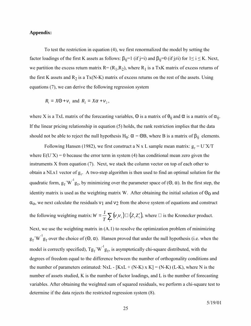
Appendix:

To test the restriction in equation (4), we first renormalized the model by setting the

factor loadings of the first K assets as follows: βij=1 (if j=i) and βij=0 (if j≠i) for 1≤ i ≤ K. Next,

we partition the excess return matrix R= (R1,R2), where R1 is a TxK matrix of excess returns of

the first K assets and R2 is a Tx(N-K) matrix of excess returns on the rest of the assets. Using

equations (7), we can derive the following regression system

11 ν+Θ= XR and 22 να += XR ,

where X is a TxL matrix of the forecasting variables, Θ is a matrix of θij and α is a matrix of αij.

If the linear pricing relationship in equation (5) holds, the rank restriction implies that the data

should not be able to reject the null hypothesis H0: α = ΘB, where B is a matrix of βij elements.

Following Hansen (1982), we first construct a N x L sample mean matrix: gT = U´X/T

where E(U´X) = 0 because the error term in system (4) has conditional mean zero given the

instruments X from equation (7). Next, we stack the column vector on top of each other to

obtain a NLx1 vector of gT. A two-step algorithm is then used to find an optimal solution for the

quadratic form, gT´W-1

gT, by minimizing over the parameter space of (Θ, α). In the first step, the

identity matrix is used as the weighting matrix W. After obtaining the initial solution of Θο and

αo, we next calculate the residuals ν1 and ν2 from the above system of equations and construct

the following weighting matrix: ( ) ( ),ZZT1W tt

ttt ′⊗= ∑ νν where ⊗ is the Kronecker product.

Next, we use the weighting matrix in (A.1) to resolve the optimization problem of minimizing

gT´W-1

gT over the choice of (Θ, α). Hansen proved that under the null hypothesis (i.e. when the

model is correctly specified), TgT´W-1

gT, is asymptotically chi-square distributed, with the

degrees of freedom equal to the difference between the number of orthogonality conditions and

the number of parameters estimated: NxL - [KxL + (N-K) x K] = (N-K) (L-K), where N is the

number of assets studied, K is the number of factor loadings, and L is the number of forecasting

variables. After obtaining the weighted sum of squared residuals, we perform a chi-square test to

determine if the data rejects the restricted regression system (8).

5/19/01 26

Table 1-- Summary Statistics

Art S&P500 Dow Gov Bond Corp Bond T-Bill

1875-1999 Mean 0.056

(0.011)

0.111 0.124 0.040 0.057 0.043

S.D. 0.256

(0.055)

0.190 0.219 0.114 0.062 0.026

1900-1999 Mean 0.047

(0.007)

0.122 0.136 0.038 0.055 0.043

S.D. 0.203

(0.064)

0.198 0.233 0.127 0.068 0.028

1950-1999 Mean 0.053

(0.002)

0.146 0.150 0.063 0.066 0.053

S.D. 0.093

(0.009)

0.165 0.168 0.099 0.091 0.030

Correlations Among Returns

Return on Art Index 1.00

Return on S&P 500 Index 0.13 1.00

Return on Dow Industrial 0.12 0.94 1.00

Return on Government Bonds -0.01 0.05 0.04 1.00

Return on Corporate Bonds -0.04 0.24 0.17 0.53 1.00

Return on Treasury Bills -0.05 -0.12 -0.13 0.17 0.25 1.00

Note: The standard errors associated with estimation error for the statistics are in the parentheses.

5/19/01 27

Table 2-- Estimation of a one-factor model (4) with pricing restriction imposed. ______________________________________________________________________________ K=1 βi1 T-Stat

______________________________________________________________________________ Estimated Beta coefficient for the following assets:

Excess return on S&P 500 Index 1.000* ----

Excess return on Art Index 0.674 3.035

Excess return on Dow Industrial 1.128 26.24

Excess return on Government Bonds 0.084 3.419

Excess return on Corporate Bonds 0.217 4.693

χ2-statistic of the rank restriction (5): 37.03 Significance level: P=0.012

______________________________________________________________________________ Notes: Asterisk(*) indicates the parameter is normalized to be one. The sample period for this

table is 1875-1999, with 125 observations.

Table 3--Tests of the Underperformance of Masterpieces

All American Impressionist Old Master

Sample Period 1875-2000 1941-2000 1941-2000 1899-2000

Panel A: Test using Nominal Value

γ -0.010 -0.010 -0.006 -0.012

t-stat -30.54 -8.071 -7.792 -28.32

Panel B: Test using Real Value

γ -0.010 -0.011 -0.005 -0.013

t-stat -30.81 -8.116 -7.467 -27.99

Note: Three-stage-generalized-least square RSR estimation of Case and Shiller (1989) are used

to estimate: ( ) ∑∑+=+=

+⋅−+=i

i

i

i

s

1btits,iii

s

1btti lnbsr εΡγµ .

5/19/01 28

Table 4--Tests of Winners Curse

Sample Period Estimation of Equation (11) and (12)

All

1875-2000 eri = 0.046 0.017*epi + ξi R2 = 0.034

(6.877) (-4.298) Obs = 494

eri = 0.090 0.012*epi 0.005*ln(Pi,b)+ ξi R2 = 0.039

(3.753) (-2.742) (-1.911) Obs = 494

All

1875-1975 eri = 0.017 0.051*epi + ξi R2 = 0.043

(0.432) (-1.951) Obs = 63

eri = -0.111 0.060*epi + 0.018*ln(Pi,b) + ξi R2 = 0.033

(-0.526) (-2.002) (0.616) Obs = 63

All

2nd purchase

made after

1975

eri = 0.035 0.014*epi + ξi R2 = 0.030

(3.204) (-2.656) Obs = 196

eri = 0.168 0.010*epi - 0.013*ln(Pi,b) + ξi R2 = 0.058

(3.215) (-1.930) (-2.606) Obs = 196

Note: T-statistics are in the parentheses. R2 have been adjusted for degrees of freedom.

Table 5--Tests of Law of One Price

All American Impressionist Old Master

Sample Period 1875-2000 1941-2000 1941-2000 1899-2000

ρ -0.001 -0.008 -0.003 -0.001

t-stat -0.976 -1.542 -1.252 -0.380 Sample Period 1950-2000 1950-2000 1950-2000 1950-2000

ρ -0.001 -0.008 -0.002 0.002

t-stat -0.234 -1.395 -0.595 0.064

Note: Three-stage-generalized-least square RSR estimation of Case and Shiller (1989) are used

to estimate: ( ) ∑∑+=+=

+⋅−+=i

i

i

i

s

btitiii

s

btti Dbsr

11ερµ , where Di is an auction house dummy.

5/19/01 29

Figure 1: Number of Observations by Purchase and by Sale

0

50

100

150

200

250

300

350

400

450

1875 1885 1895 1905 1915 1925 1935 1945 1955 1965 1975 1985 1995

Obs

erva

tions

PurchaseSale

5/19/01 30

Figure 2: Nominal Indexes

(Base Year: All 1875=100, American 1941=100, Impressionist 1941=100, Old Master 1899=100)

Notes: For the All Art Index, regression statistics for the three-stage-generalized-least square

RSR estimation of Case and Shiller: R2=0.64, F(125,4771) =120.62 with a significance level

equal to 0.000. Annualized returns are computed as exp(µt + σ2/2)-1, σ2 is estimated in the

second stage of RSR.

5/19/01 31

Figure 3: Old Master Paintings Resale Returns

-60%

-40%

-20%

0%

20%

40%

60%

80%

$1 $10 $100 $1,000 $10,000 $100,000 $1,000,000 $10,000,000

PURCHASE PRICE

5/19/01 32

Figure 4: The Relationship between Excess Payment and Future Excess Returns

-100%

-50%

0%

50%

100%

150%

200%

-6 -4 -2 0 2 4 6 8

Log(Excess Payments)

Exce

ss R

etur

ns